Article

A Multi-Dimensional Indicator Framework for Peri-Urban Area Delineation: Insights from Equal- and AHP-Weighted Models in Java, Indonesia


by
Ziyue Wang
1,
Adhitya Marendra Kiloes
1,2,
Md. Ali Akber
1,
Bagus Setiabudi Wiwoho
3 and
Ammar Abdul Aziz
1,*
1
School of Agriculture and Food Sustainability, The University of Queensland, Gatton, QLD 4343, Australia
2
Research Center for Behavioral and Circular Economics, National Research and Innovation Agency of the Republic of Indonesia (BRIN), Jakarta 12710, Indonesia
3
Department of Geography, Universitas Negeri Malang, Malang 65145, Indonesia
*
Author to whom correspondence should be addressed.
Remote Sens. 2026, 18(7), 1062; https://doi.org/10.3390/rs18071062
Submission received: 22 February 2026 / Revised: 24 March 2026 / Accepted: 28 March 2026 / Published: 2 April 2026

Highlights

What are the main findings?
  • An 18-indicator GIS-based framework generates continuous peri-urban probability surfaces.
  • Equal-weighted integration shows higher validation accuracy than AHP weighting.
What are the implications of the main findings?
  • Remote sensing and GIS enable spatially explicit monitoring of peri-urban gradients.
  • The transferable workflow supports scalable peri-urban mapping in rapidly urbanizing regions.

Abstract

Peri-urban areas (PUAs), as transitional zones between urban and rural regions, play a critical role in supporting food systems and agricultural livelihoods, yet they are increasingly pressured by rapid urban expansion. Reliable spatial delineation of PUAs remains challenging, as administrative boundaries often fail to capture their functional and spatial heterogeneity. This study proposes a multi-dimensional, spatially explicit framework to delineate peri-urban areas using Indonesia as a case study. Eighteen indicators representing six analytical dimensions—land use/land cover, economic, demographic, infrastructural, spatial accessibility, and landscape structure—were derived from remote sensing and GIS-based data sources and integrated into a composite scoring system using equal-weighted and AHP-weighted approaches. The framework was applied to four major cities on Java Island (Jakarta, Surabaya, Bandung, and Yogyakarta) to generate continuous peri-urban probability surfaces, which were validated using expert surveys across 25 districts in the Jakarta and Bandung metropolitan areas. The results show that the framework effectively captures the spatial heterogeneity and gradients of peri-urban areas, with the equal-weighted approach exhibiting statistically significant agreement with expert assessments (Pearson’s r = 0.517, p = 0.008; Spearman’s ρ = 0.522, p = 0.008; Kendall’s τ = 0.387, p = 0.008), consistently outperforming the AHP-weighted model across all validation metrics. The proposed approach provides a transferable spatial mapping framework for monitoring peri-urban dynamics in rapidly urbanizing regions using remote sensing and GIS.

1. Introduction

The world is undergoing an unprecedented phase of urbanization, a process that is reshaping landscapes, economies, and livelihoods across regions [1,2]. By 2030, the global urban land area is projected to almost triple, from 0.65 million km2 in 2000 to 1.86 million km2 [3]. This accelerated spatial expansion has prompted both rapidly growing metropolitan regions and formerly industrialized “rust belt” cities to extend their urban footprints into surrounding rural hinterlands [4,5]. As a result, peri-urban areas (PUAs) have emerged as dynamic transitional interfaces between urban and rural regions, shaped by the ongoing pressures of urban growth [6], thereby posing new challenges for sustainable planning and agricultural resilience.
In developing countries, peri-urban agriculture plays a crucial role in sustaining agricultural functions, providing local food production, ecosystem services, and socioeconomic benefits [7]. However, the growing pressures of rapid urban expansion, coupled with weak regulatory measures, threaten these agricultural systems by intensifying land-use conflicts and resource competition [8]. This unchecked development often leads to tensions between urban development and agricultural land use, as expanding construction projects and infrastructure encroach on farmland, driven by competing land use priorities [9]. Furthermore, the spatial heterogeneity and indistinct boundaries of PUAs complicate effective management and regulatory intervention [10]. Given the crucial role peri-urban agriculture plays and the growing pressures it faces, it is necessary to incorporate agricultural and functional dimensions into the delineation of peri-urban areas. Such an approach would enable more targeted protection of agricultural land and promote balanced, sustainable urban growth. In rapidly urbanizing areas such as Java, Indonesia, peri-urban agriculture plays a critical role in supporting both local economies and urban food security [11].
Research on the identification of PUAs dates to the 19th century, when studies on urban boundaries began to emerge. Early urban geographers, such as Herbert Louis, observed that urban growth was often constrained by enduring physical and environmental boundaries [12]. Initial efforts to define urban–rural interfaces were largely qualitative, seeking to address conceptual ambiguities and social dimensions of peri-urban change rather than spatial delineation [13]. Due to variations in the radiative capacity of urban areas across different cities and periods of expansion, the spatial structure of PUAs differs significantly. As a result, methods based on empirical experience often assume spatial homogeneity, leading to subjective and qualitative identification. With the development of the conceptual theory of peri-urbanization and the improvement of geographic information technology and mathematical modeling methodology, scholars have progressively focused on the spatial identification of PUAs from qualitative description to quantitative analysis [10].
Current quantitative methods can be broadly classified as indicator-based, remote sensing-based, and sample-based methods. Remote sensing-based unsupervised methods delineate urban and rural boundaries by distinguishing and grouping the pixels with unsupervised algorithms. Peng et al. [14] broke down data into various frequency components to capture patterns at different scales by wavelet transformation and then smoothed data to show density and peri-urban distribution patterns with kernel density estimation. However, these methods often rely on visually identifying sudden changes and connecting them with straight lines, which can result in lower accuracy and require further refinement. Sample-based supervised classification methods utilize machine or deep learning models to train on numerous samples, thereby identifying urban and rural areas. Wang et al. [15] proposed a novel transferable convolutional neural network (FR-Net) for identifying PUAs in the Beijing–Tianjin–Hebei urban agglomeration in China. However, such methods are usually constrained by the difficulty of obtaining many high-quality training samples and by the poor interpretability of the model.
Compared to sample-based classification methods and remote sensing-based methods, indicator-based methods use the selected indicators to do regression analysis, factor analysis, and multivariate analysis, or use continuity methods. Regression analysis includes logistic regression to estimate relationships between variables (e.g., the effect of different forces on land use) [16,17], ordinary least squares regression [18], and geographically weighted regression to examine spatial variation [19,20]. Factor and multivariate analysis can reduce large datasets into a few meaningful parameters, often through hierarchical analysis processes like the Analytic Hierarchy Process (AHP) [21,22] and its fuzzy version (FAHP) for decision-making [23]. Continuity methods assess the degree of coordinated changes between variables using one-equation or multi-equation methods, often within simultaneous equation models [24,25]. They can provide greater flexibility by allowing researchers to incorporate both spatial and socioeconomic factors, making it more suitable for capturing the complexity of PUAs [26]. In addition, indicator-based methods require less reliance on large, high-quality training datasets, unlike sample-based supervised classification methods, and this makes them more adaptable in data-scarce environments [21].
While existing studies have largely relied on administrative boundaries to define PUAs, such approaches may overlook key agricultural zones that are integral to the region’s sustainability [11,27]. To address this limitation, this study delineates PUAs in Java by integrating economic, social, and environmental dimensions. Compared to remote sensing or sample-based approaches, indicator-based methods provide greater flexibility in capturing the multi-dimensional characteristics of PUAs, which are essential for understanding complex peri-urban dynamics. However, despite their broad applicability, current indicator-based studies share two critical methodological limitations. First, most frameworks implicitly assume that all indicators contribute equally to peri-urban characteristics, adopting uniform weights without theoretical justification or empirical validation. Little research has examined whether indicators differ in their relative importance or compared alternative weighting schemes for PUA delineation. Second, indicator-based methods are rarely subjected to external validation; the delineated boundaries are often taken as given, with few studies assessing their consistency with expert judgments or on-the-ground knowledge.
To overcome these gaps, this study develops two weighting models—an equal-weighted model and an AHP-based model—to evaluate whether different weighting strategies influence the delineation of peri-urban areas. In addition, an expert scoring (Q-score) validation framework is introduced to provide an independent reference against which model outputs can be assessed. By integrating multi-dimensional indicators with a transparent validation mechanism, this study offers the first empirical comparison of weighting strategies for indicator-based peri-urban delineation in Java. The proposed framework enhances methodological robustness and provides a transferable approach for identifying peri-urban areas in other rapidly urbanizing regions. The results provide policymakers and planners with an evidence-based tool to better manage land use transitions, balance urban expansion with agricultural sustainability, and support integrated regional planning.

2. Data and Methods

The delineation of PUAs was carried out in the following steps: (1) scoping the boundary of the PUAs, (2) developing an indicator system, (3) establishing scoring models, (4) PUA mapping, and (5) validating the PUA scoring models. The workflow is shown in Figure 1.

2.1. Study Area

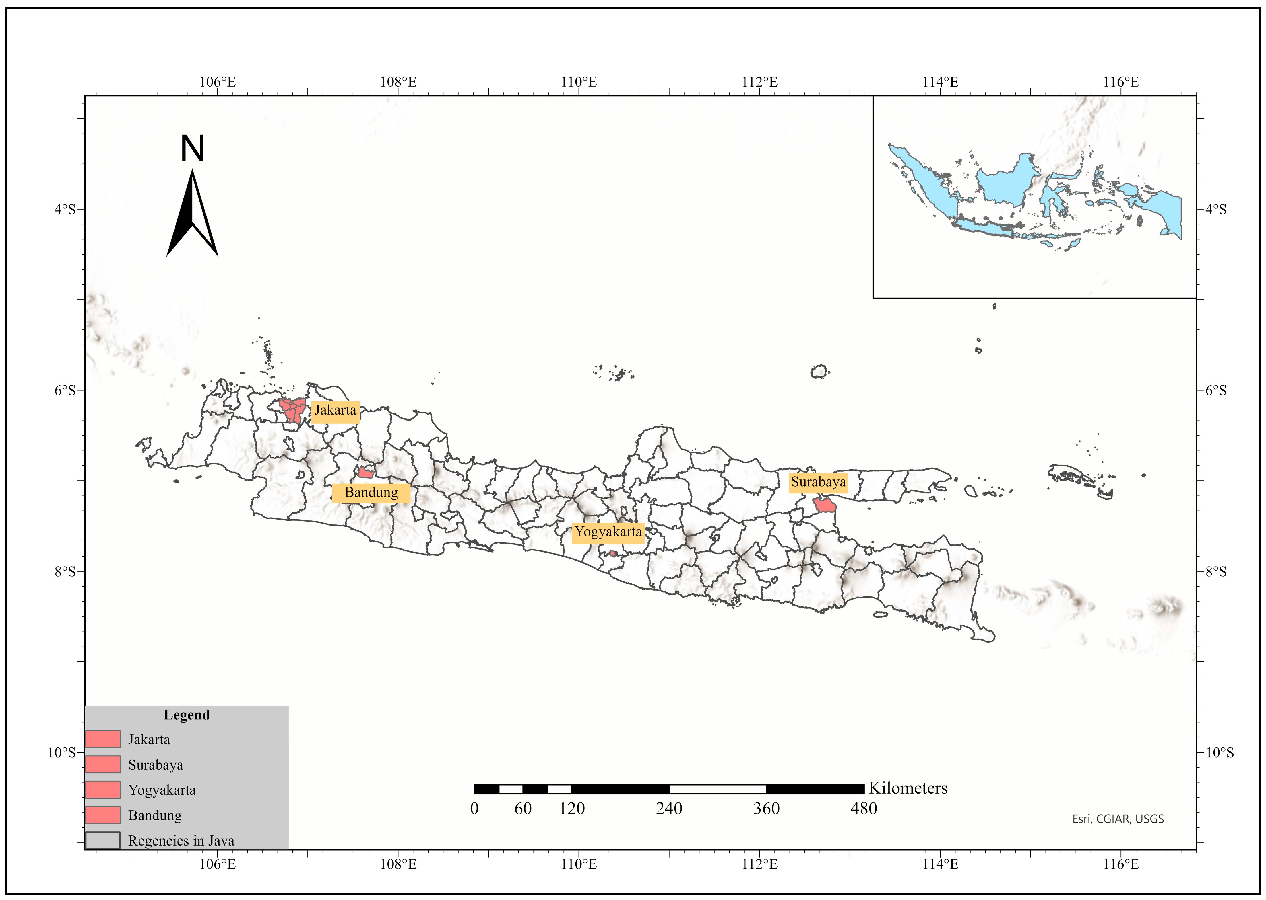
The study area of this research is based on Java Island, situated in the heart of Indonesia (Figure 2). Java Island is divided into four administrative provinces, Banten, West Java, Central Java, and East Java, and two special regions, Jakarta and Yogyakarta. The area of Java Island is around 128,297 km2, occupying only 7% of the total land area of the republic. Due to a tropical climate with relatively high temperatures, plenty of sunlight throughout the year, and relatively humid climate conditions, an environment conducive to diverse and abundant crop cultivation is created, and more than two-thirds of the island’s area is under cultivation. Despite occupying only 7% of Indonesia’s land area, Java is home to approximately 152 million people as of 2023, accounting for more than 50% of the country’s total population of roughly 277 million [28]. Agriculture serves as a cornerstone of livelihoods for many.
The study focuses on the mapping of PUAs in Java Island, Indonesia, concentrating on its four major urban centers, Jakarta, Surabaya, Bandung, and Yogyakarta (shown in Figure 2), which belong to the Special Capital Region of Jakarta, East Java, West Java, and the Special Region of Yogyakarta. These cities are among the top four most densely populated cities on Java Island, facing increasing urban sprawl and land use change.

2.2. Data Collection

2.2.1. Secondary Data

This study combined multiple data sources to construct and validate the PUAs’ scoring system. First, the data needed for this research is meticulously selected in alignment with the predefined set of indicators essential for our analysis. We have sourced all the required data exclusively from publicly accessible datasets made available through various online platforms. This approach ensures transparency and reproducibility of the research findings. To aid in understanding and verification, a detailed table is provided that lists each specific dataset used along with its corresponding source. Table A1 includes comprehensive information on the data and its source.

2.2.2. Questionnaire Survey Data

In addition to secondary data, an expert questionnaire survey was conducted to integrate domain knowledge into both the development and validation of the scoring model. The questionnaire was administered via Qualtrics and distributed among researchers, local government officers, and farmers across in Java Island, combining professional expertise and local experiential knowledge. Respondents were selected based on their professional expertise or direct involvement in urban planning, land use management, and agricultural practices, ensuring representation of both technical and community perspectives. A total of 146 valid responses were collected. This research was approved by the University of Queensland Human Research Ethics Committee, and all participants provided informed consent.
The questionnaire consisted of two sections. The first section required pairwise comparisons of indicators, which were analyzed using the AHP method to derive relative indicator weights for constructing the weighted PUA-scoring model (see Section 2.5.2). The second section collected district-level expert assessments of peri-urban characteristics, which served as reference values for validating the model outputs (see Section 2.7).
For model validation, Jakarta and Bandung were selected as case sites for two main reasons. First, Jakarta and Bandung capture contrasting yet representative urban contexts in Java. Jakarta, as Indonesia’s primary megacity, exemplifies intense metropolitan expansion and complex peri-urban dynamics [29,30], while Bandung represents a medium-sized, rapidly growing regional center in a mountainous environment, where peri-urbanization is shaped by both topography and tourism-driven development [31]. Additionally, both cities are closely linked within the Java Economic Corridor under Indonesia’s Master Plan for the Acceleration and Expansion of Economic Development (MP3EI), with major infrastructure investments such as the Jakarta–Bandung high-speed rail enhancing inter-city connectivity [32]. This combination of data availability, representativeness, and regional integration makes Jakarta and Bandung particularly suitable as testbeds for model validation. Second, surveying experts across all 767 districts within the buffer zones of four cities was not feasible, given the logistical constraints of field-based questionnaire distribution in Indonesia. Focusing on Jakarta and Bandung provided a manageable yet representative scope for validation. This combination of representativeness, regional integration, and practical feasibility makes Jakarta and Bandung particularly suitable as testbeds for model validation.
To contextualize the validation scope, it is necessary to clarify Indonesia’s administrative hierarchy. At the national level, the country is divided into provinces (first-level administrative divisions). The provinces below are regencies (Kabupaten, generally rural) and municipalities (Kota, primarily urban) as second-level units. Each is further subdivided into districts or sub-districts (Kecamatan), the third-level administrative units referred to as “districts” in this study. Jakarta is a province-level municipality comprising five municipalities (West, North, Central, South, and East Jakarta) and one regency (Kepulauan Seribu). Bandung refers to the capital municipality (Kota Bandung) of West Java Province, which is adjacent to—but administratively separate from—Bandung Regency (Kabupaten Bandung) [28,33].
The combined area of Jakarta and Bandung contains approximately 416 districts. To determine the minimum number of districts required for a statistically representative sample, Cochran’s formula was applied with a 95% confidence level (Z = 1.96), maximum variance (p = 0.5), and a margin of error of 15%, yielding a minimum sample size of 48 districts. Since the equal-weighted model relies solely on remote sensing and GIS-derived indicator data and does not require questionnaire input, it was computed prior to the survey to provide a preliminary spatial assessment of peri-urban characteristics across all 416 districts. A stratified random sampling approach was then applied to select the 48 districts for the survey, with districts stratified into three groups based on their equal-weighted model scores (high: ≥65, medium: 52–63, low: ≤51) to ensure that the validation sample captured the full spectrum of peri-urban characteristics. The number of districts selected from each stratum was proportional to its share of the total, ensuring that sampled districts represented contrasting urban–rural gradients and diverse peri-urban contexts.

2.3. Conception of PUAs and the Scope of the Boundary of PUAs

PUAs are conceptually understood as zones delineated by two dynamic boundaries. The inner boundary is situated at the edge of the urban area, while the outer boundary extends into the rural landscape [10]. In the context of Asian countries, particularly Indonesia, PUAs are predominantly located within metropolitan regions but typically fall outside formal urban boundaries, such as those defined by municipalities and city councils, as well as outside urban jurisdictions [21,34].
Based on this conceptualization, the delineation of PUAs requires the establishment of two distinct boundaries. The first boundary marks the urban edge, defining the limit of the core urban area. To determine this boundary, the outer limits of settlement for four cities were compared with their administrative areas, and it was found that these boundaries almost overlap due to the high level of urbanization. Therefore, the administrative area with smoother borders is selected as the inner boundary. The second boundary, however, extends beyond traditional metropolitan limits. Due to the expansive geographic coverage of regencies in Java, peri-urbanization tends to cluster disproportionately along key corridors rather than uniformly extending outward from the core [21]. This uneven distribution is often distorted when using administrative boundaries, as such boundaries average out the more concentrated effects of peri-urbanization [35]. Consequently, we adopt a 50 km threshold for the outer boundary of four cities to do buffer analysis in ArcGIS Pro. Moreover, 50 km has been widely recognized as reasonable in Southeast Asian contexts. This distance, as used in this study, aligns with Webster, Cai, Muller and Luo’s [35] and McGee’s [36] proposals for setting the peri-urban boundary 50 km from the city center, while Webster, Cai, Muller and Luo [35] suggested that PUAs typically extend 30–50 km beyond the established urban limits.

2.4. Indicator System and Data Processing

2.4.1. Indicator Selection

Indicators are measurable metrics and are used to directly measure the intensity and scale of various factors of PUAs. In previous studies, indicators for mapping PUAs varied depending on the desired objectives and stakeholder requirements in several principal types of background: land use planning, environment/climate/farm policies, and socioeconomic aspects of urban and rural areas [10]. Danielaini, Maheshwari and Hagare [21] selected indicators directly and indirectly, using some indications of ecohydrology to delineate PUAs in the Cirebon Metropolitan Region of West Java. However, Kontgis et al. [37] conducted a statistical analysis of land cover indicators and Demographic indicators for urban and PUAs in the greater Ho Chi Minh City metropolitan area in the context of urban and rural planning.
These indicators are often argued in the form of physical, socioeconomic, and ecological factors [4]. Physical factors primarily refer to the tangible changes in the environment, and are based on the variables of land use change/land cover [22,38], spatial character change, which refers to the transformation of peri-urban spatial morphology over time, driven by various factors, particularly under the influence of urban sprawl and development pressure [39,40] and built-up density [41,42]. The socioeconomic factor refers to the social and economic dynamics that influence PUAs, which are primarily based on three key variables: population change, which tracks shifts in the number of residents [21,43,44,45,46]; employment opportunities, which assess the availability and distribution of jobs [47]; and the value of land and housing, which measures fluctuations in property prices and land costs within the region [48,49]. The ecological factors of PUAs are often associated with the spatial structure of landscape composition and the valuable natural environments to provide essential ecosystem functions for residents [50].
This article aims to define PUAs in a manner that is suitable for application across disciplines while also addressing the region-specific context of Java Island. Therefore, the selection of indicators for peri-urban mapping was guided not only by a comprehensive perspective but also by empirical evidence from previous studies. In this study, six categories of indicators were identified to capture the multifaceted nature of PUAs: LULC, EF, DF, IF, SA, and LS. These six dimensions can be mapped to the three factor categories: physical factors (LULC, LS), socioeconomic factors (EF, DF, IF), and spatial accessibility factors (SA). The formula of each indicator and the data sources are summarized in Table 1.
LULC indicators capture the transitional land cover composition characteristic of peri-urban areas, which typically exhibit intermediate levels of built-up density, cropland, vegetation, and impervious surfaces compared to urban cores and rural hinterlands. Specifically, LULC indicators include Proportion of Build-up Area (PBU), Proportion of Crop Area (PCR), Build-up Growth Rate during 2010 to 2020 (BGG), Proportion of Green Vegetation Fraction (BVF), Proportion of Impervious Surface Fraction (ISF), and Proportion of Forest Area (PFA). These indicators are well-documented in the literature for PUA delineation and have been validated by studies [21,44,51].
The EF indicators were used to reflect the economic vitality of cities and their surrounding area. Peri-urban zones typically exhibit more diversified economic activities than rural areas but less concentrated than urban cores, and this intermediate economic profile can be captured by Number of Economic Resources per area (NEI) and Night Light Intensity (NLI). Population Density (PDB) and Population Growth Rate (PGG) are the two demographic indicators selected in this study, which reflect the population relationship between a city and its surrounding area. PDB is a fundamental measure of urbanization, which is a characteristic feature of urban regions. PGG is a typical indicator of urban dynamics, and a higher growth rate indicates increased urbanization. The higher possibility of PUAs is led by the higher PDB and PGG surrounding the city. IF indicators, including Arterial Road density (ART), Collector Road Density (CRD), Local Road Density (LRD), and Number of Public Facilities per area (NFP), reflect the transitional infrastructure provision of peri-urban areas, which typically have lower road density and fewer public facilities than urban areas but higher levels than rural areas [43].
SA indicators comprise Distance to City Center (DTC) and Distance to Forest (DTF). DTC captures the spatial positioning of districts relative to the urban core, while DTF reflects proximity to natural landscapes; peri-urban areas are characteristically situated at intermediate distances from both, distinguishing them from core urban and remote rural zones.
The importance of these indicators is supported in previous studies [21,43,44,45,46,51,52,53,54], which demonstrated their relevance in peri-urban detection. Finally, LS indicators were assessed using Build-up Landscape Patch Density (BPD) and Patch Density (PDN), which reflects the degree of urban sprawl and discontinuous development, thereby indicating the expansion of cities into peri-urban regions. PDN measures the overall landscape fragmentation, with peri-urban areas typically exhibiting higher patch density than either compact urban cores or extensive rural landscapes. Previous studies provide substantial evidence of its utility in analyzing urban form and spatial organization [37,55].

2.4.2. Data Standardization

Scaling the indicators with different units was to transform them into a standardized format, typically expressed as a percentage. Data scaling is essential because the indicators being used come from different domains and have different units of measurement (e.g., population density, land use percentages, and economic factors). By converting all indicators into a standard scale, such as percentages, we ensure that each variable contributes equally to the scoring system, making it possible to perform valid comparisons and draw meaningful conclusions [56]. Additionally, this normalization process ensures comparability across districts of varying sizes within this study. For instance, the NLI (Night Light Intensity) indicator represents relative data, where the level of density within different districts of a province is measured against the provincial reference, rather than the entire study area. Scaling adjusts for such differences by converting raw data into a format that is independent of local scale while still capturing local characteristics. This step is essential for ensuring fair comparisons and accurate analysis. In this study, 11 indicators (NEI, NLI, PDB, ART, CRD, LRD, NFP, DTC, DTF, BPD, PDN) were grouped according to the four provinces, and Min–Max normalization, which rescales the range of values to [0, 100%], was applied to standardize the data.

2.4.3. Scoring System for Indicators

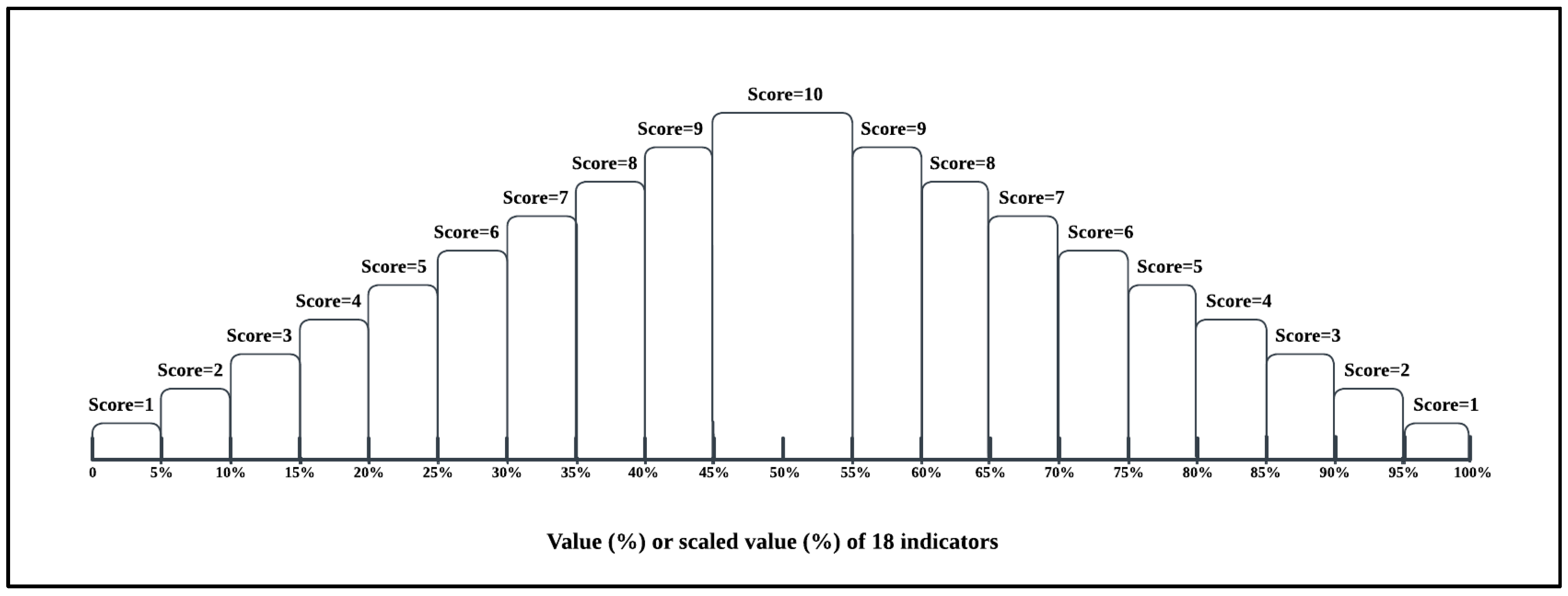
According to the previous studies [21,44,53,57], when the value or scaled value of various indicators hovers around 50%, they are most likely to capture the defining characteristics of PUAs. A 1–10 scoring system was adopted for its ability to provide adequate sensitivity, allowing for the detection of subtle differences between indicators without introducing unnecessary complexity, and facilitates standardized comparisons across various indicators, ensuring consistency in evaluation regardless of their original measurement scale [58]. The scoring system divides the standardized indicator range (0–100%) into uniform intervals of 5 percentage points, following a symmetric distribution centered on the 50% midpoint. Indicator values falling within the 45–50% and 50–55% intervals receive the highest score of 10, while scores decrease progressively toward both extremes, with values near 0% or 100% receiving the lowest score of 1. The PUAs’ thresholds and scoring system for the 18 indicators are detailed in Figure 3, ensuring that the evaluation aligns with the typical traits of peri-urban regions. It should be noted that the scoring logic itself—assigning higher scores to intermediate indicator values that characterize transitional peri-urban zones—is conceptually transferable, as it is rooted in the general definition of PUAs as zones between urban and rural extremes. However, the specific threshold breakpoints were calibrated to the Indonesian context using Min–Max normalization within provincial groupings (see Section 2.4.2). When applying this framework to other countries or regions, the thresholds would need to be recalibrated based on local data distributions, as the ranges of indicator values (e.g., population density, built-up area proportion) vary significantly across geographic contexts.

2.5. PUA Scoring Model Development

To translate the standardized indicators into a composite measure of peri-urbanity, two scoring models were developed: an equal-weighted model and an AHP-weighted model incorporating expert-derived weights. These two approaches provide complementary perspectives, one offering a neutral baseline free from subjective bias, and the other reflecting contextual knowledge and priorities expressed by domain experts.

2.5.1. Equal-Weighted Model Construction

The equal-weighted model was designed to serve as an objective benchmark. In this approach, all indicators were assigned identical weights, such that the final PUA score of district i was obtained as the arithmetic sum of its standardized indicator scores:
P U A i = j = 1 n S i j
where P U A i denotes the score of district i, S i j   is the standardized score of indicator j for district i, and n is the total number of indicators. By treating each indicator as equally important, this model eliminates the potential influence of subjective preferences, thereby providing a transparent and replicable baseline for subsequent comparison.

2.5.2. AHP-Weighted Model Construction

To complement the equal-weighted approach, an AHP-weighted model was established to embed expert judgment into the evaluation framework. Weighting information was derived from an AHP questionnaire, which was administered via Qualtrics and distributed among researchers, local government officers, and farmers. In this way, both professional expertise and local experiential knowledge were incorporated. A total of 146 responses were obtained from 48 districts. Each response generated a pairwise comparison matrix, and following the AHP consistency criterion, matrices with a consistency ratio (CR) lower than 0.1 were retained, leaving 80 valid responses from 25 districts.
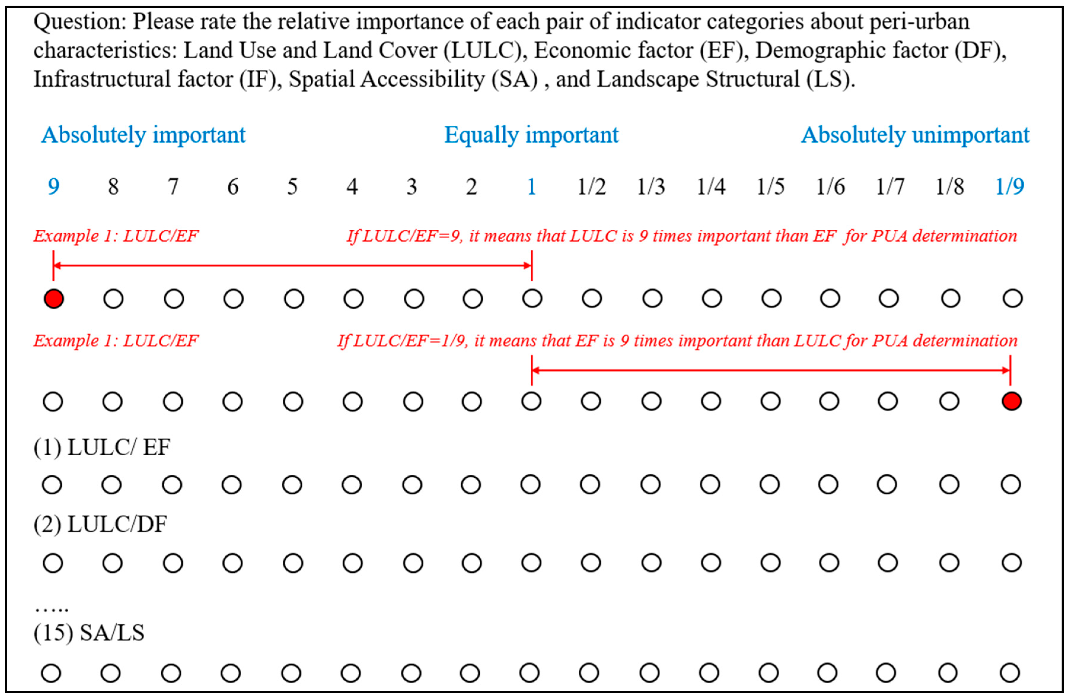
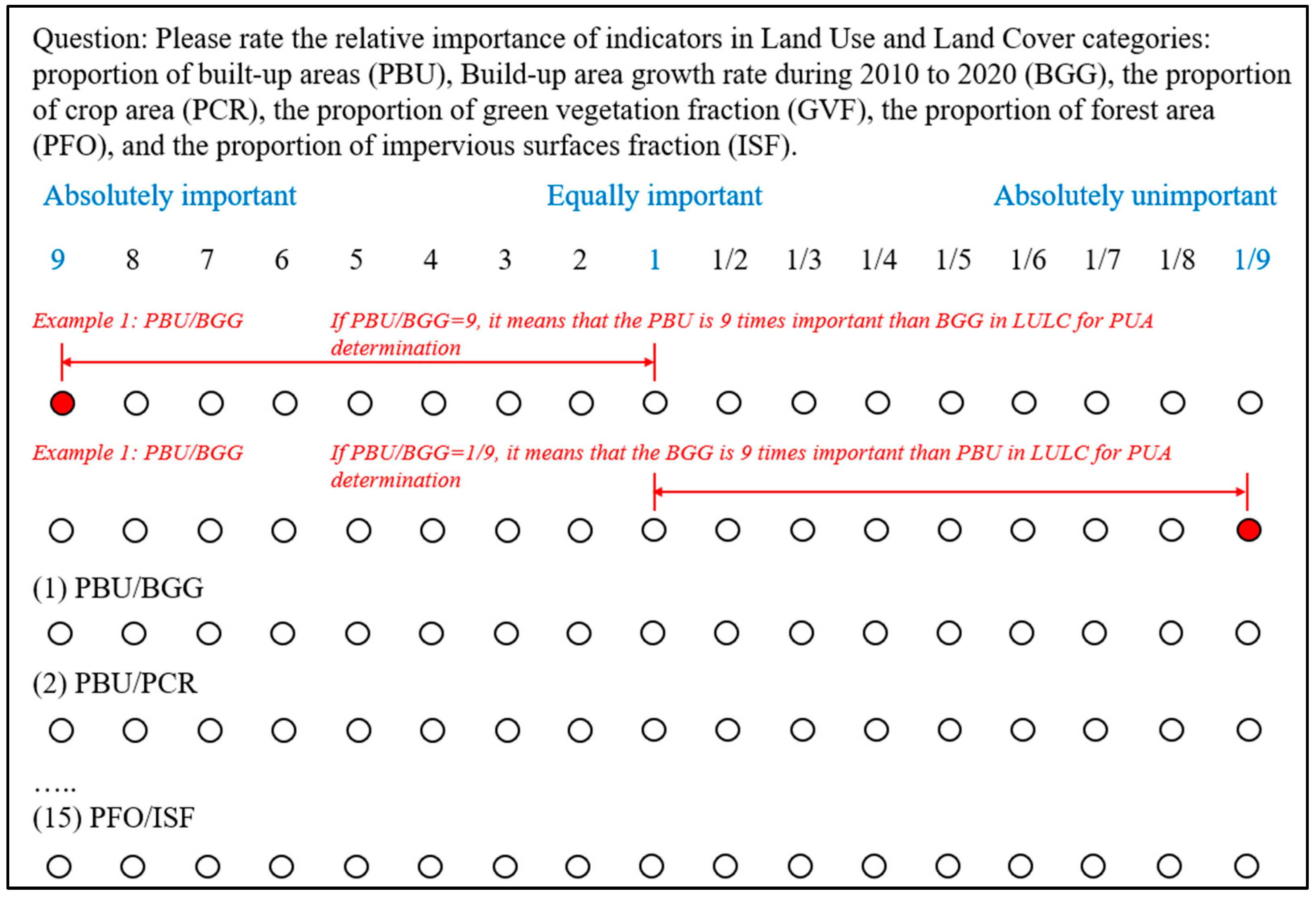
The questionnaire was designed with a hierarchical structure to ensure that the weighting process could capture both broad categories and detailed sub-indicators. At the primary level, experts were asked to compare the relative importance of six major indicator categories—DF, LULC, EF, IF, SA, and LS—using the standard 1–9 AHP scale (Figure 4). At the secondary level, the same pairwise comparison procedure was applied within each category to refine the weights of sub-indicators. For instance, within the LULC category, experts compared six variables: PBU, BGG, PCR, GVF, PFA, and ISF (Figure 5).
For each district, valid responses were aggregated using the geometric mean method to generate a collective comparison matrix. The normalized principal eigenvector of this aggregated matrix provided the final set of weights ( w j ) ensuring that j = 1 n w j = 1 . The composite PUA score for district i was then calculated as:
P U A i = j = 1 n w j S i j , where   j = 1 n w j = 1
where S i j represents the standardized score of the indicator j for district i. This formulation allowed indicators considered more critical by experts to exert proportionally greater influence on the final district scores, thereby embedding domain knowledge and contextual understanding into the model and providing an alternative perspective to the equal-weighted benchmark. The resulting weight coefficients for both the primary- and secondary-level indicators are summarized in Table 1 and were used as input parameters for the subsequent calculation of PUA scores.

2.6. PUA Mapping

The next step involves classifying each district based on its peri-urban score. The Jenks Natural Breaks method was selected for this classification, which is widely recognized in GIS for its ability to identify spatial patterns in attribute distributions across regions through statistically optimized classification. This approach, based on Jenks’ optimization, was derived from Fisher’s method [59,60]. In this study, this method was used to generate three distinct classes: high, medium, and low peri-urban potential. The class breaks were determined by grouping similar values together while maximizing the differences between classes. Subsequently, districts were categorized based on these breaks, with class boundaries set at points where there were relatively large variations in data values. The final results were mapped by ArcGIS Pro version 3.0.2, developed by the Environmental Systems Research Institute (ESRI).

2.7. PUA Scoring Model Validation

For the validation analysis, as described in Section 2.2.2, Jakarta and Bandung were selected as validation sites based on their representativeness and a statistically grounded sampling design. Questionnaires were distributed across 48 districts selected through stratified random sampling, yielding a total of 146 responses. Each response produced an AHP pairwise-comparison matrix that was screened for logical consistency. Following the AHP criterion (CR < 0.1 at all hierarchy levels), 80 valid responses from 25 districts were retained as the quality-controlled set for validation.
For each valid district, individual expert ratings were averaged to obtain a single district-level reference score, reflecting the collective judgment of experts. This district-level expert reference score is hereafter denoted as Q-score. The Q-score reflects a holistic assessment of peri-urban characteristics at the district level and is derived independently of the indicator weighting process used in the AHP model. As such, it serves as a perception-based reference for validation rather than a direct evaluation of the model inputs. We then compared model-derived PUA scores (from both the equal-weighted and AHP-weighted models) against these expert-based reference scores using Pearson’s r, Spearman’s ρ, and Kendall’s τ. Kendall’s τ was included as a complementary rank-based metric that is more robust for small sample sizes. In response to a re-examination of the validation procedure, correlation coefficients were computed directly between raw model outputs and raw expert reference scores without prior scale calibration, as all three metrics are inherently scale-invariant. The model-derived peri-urban likelihood score is hereafter denoted as Mscore. Error-based metrics (e.g., RMSE, MAE) and categorical indices (e.g., Kappa) were not emphasized because expert ratings constitute reference assessments rather than strict ground truth; our focus was on trend consistency rather than point-wise numerical agreement. In addition, a cross-tabulation analysis was conducted to quantify the classification agreement between the equal-weighted and AHP-weighted models, and the mean indicator scores were compared across the four metropolitan areas to examine cross-city variability in peri-urban characteristics.

3. Results

3.1. Mapping PUA Boundaries Across Four Cities

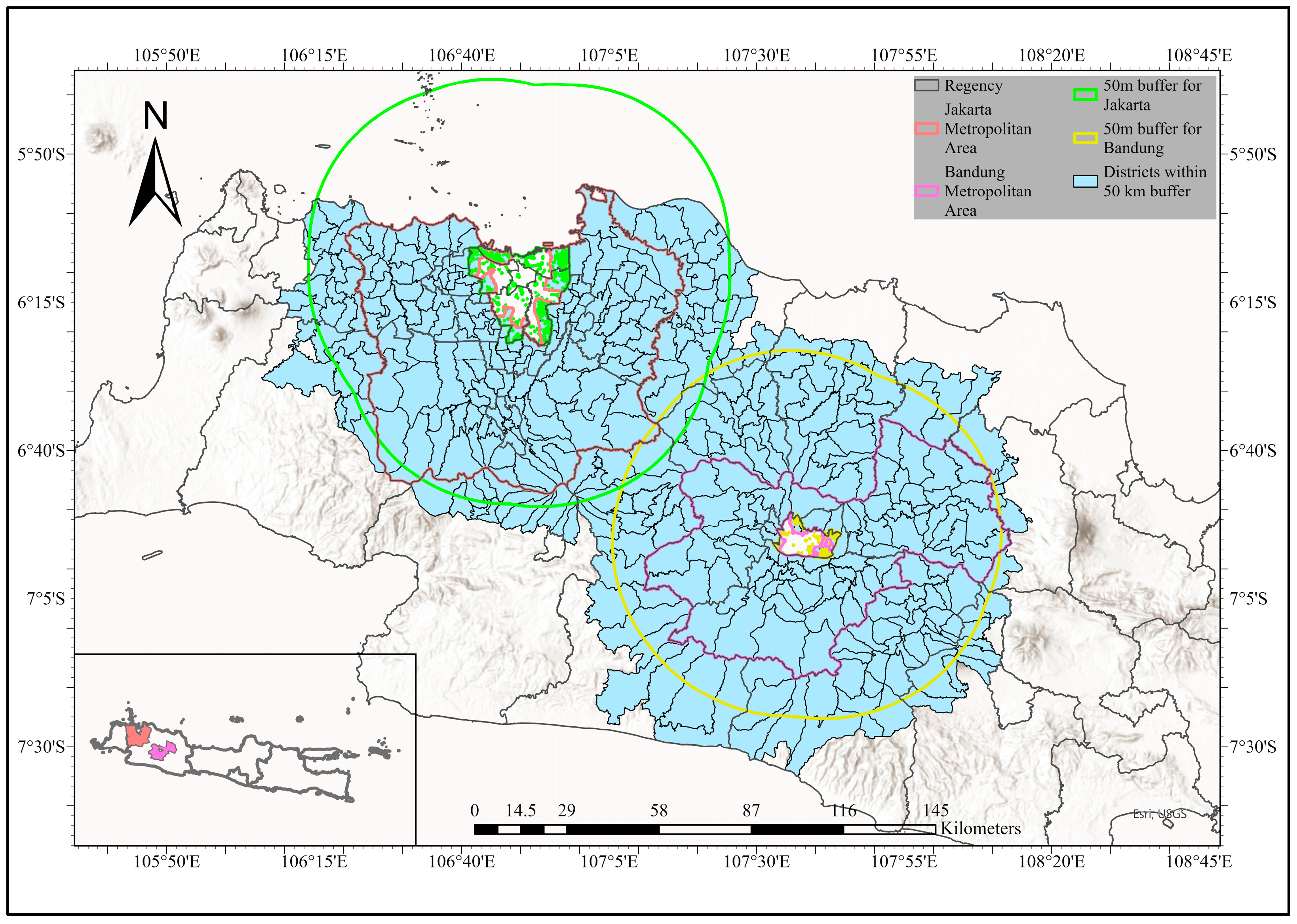
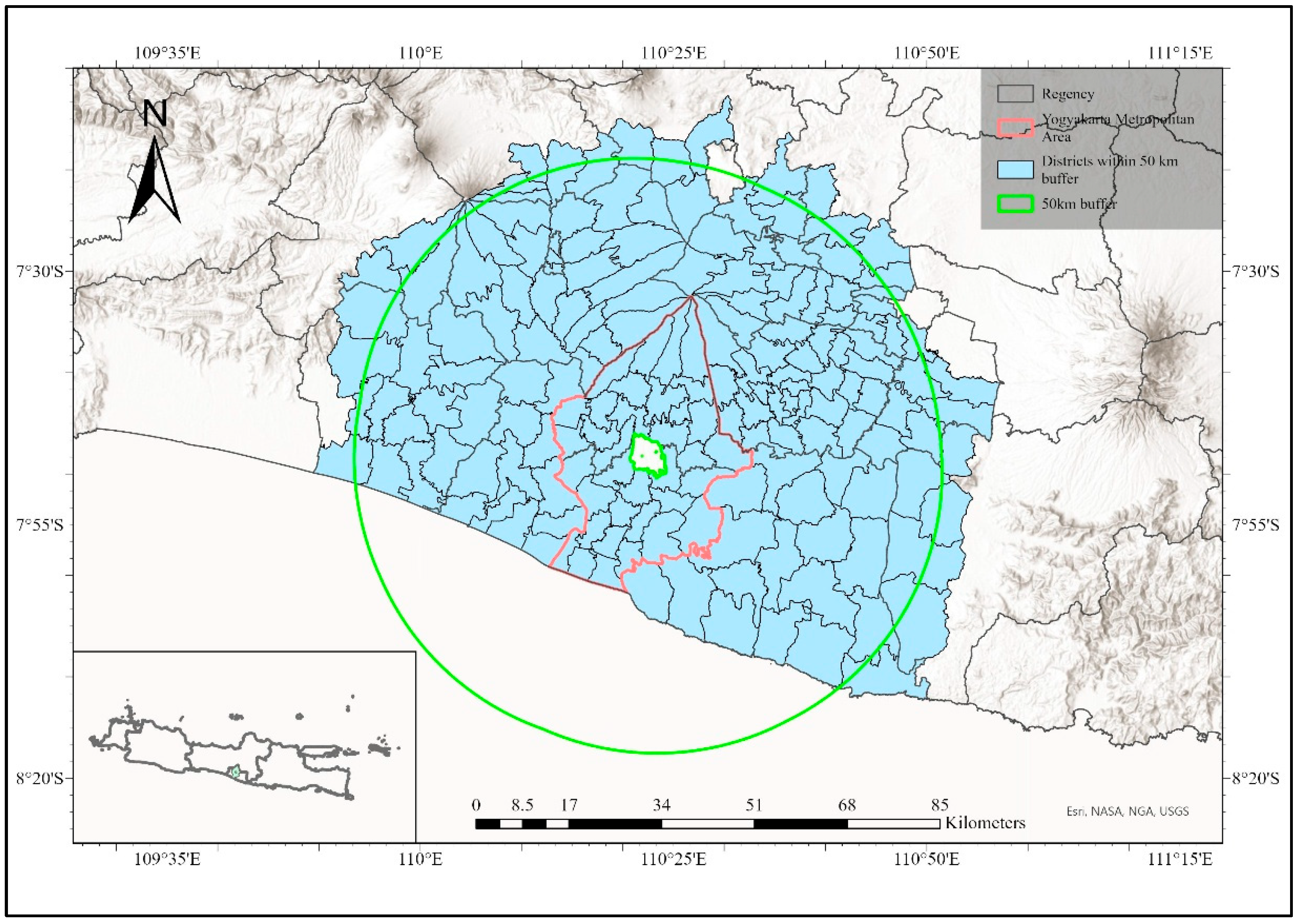
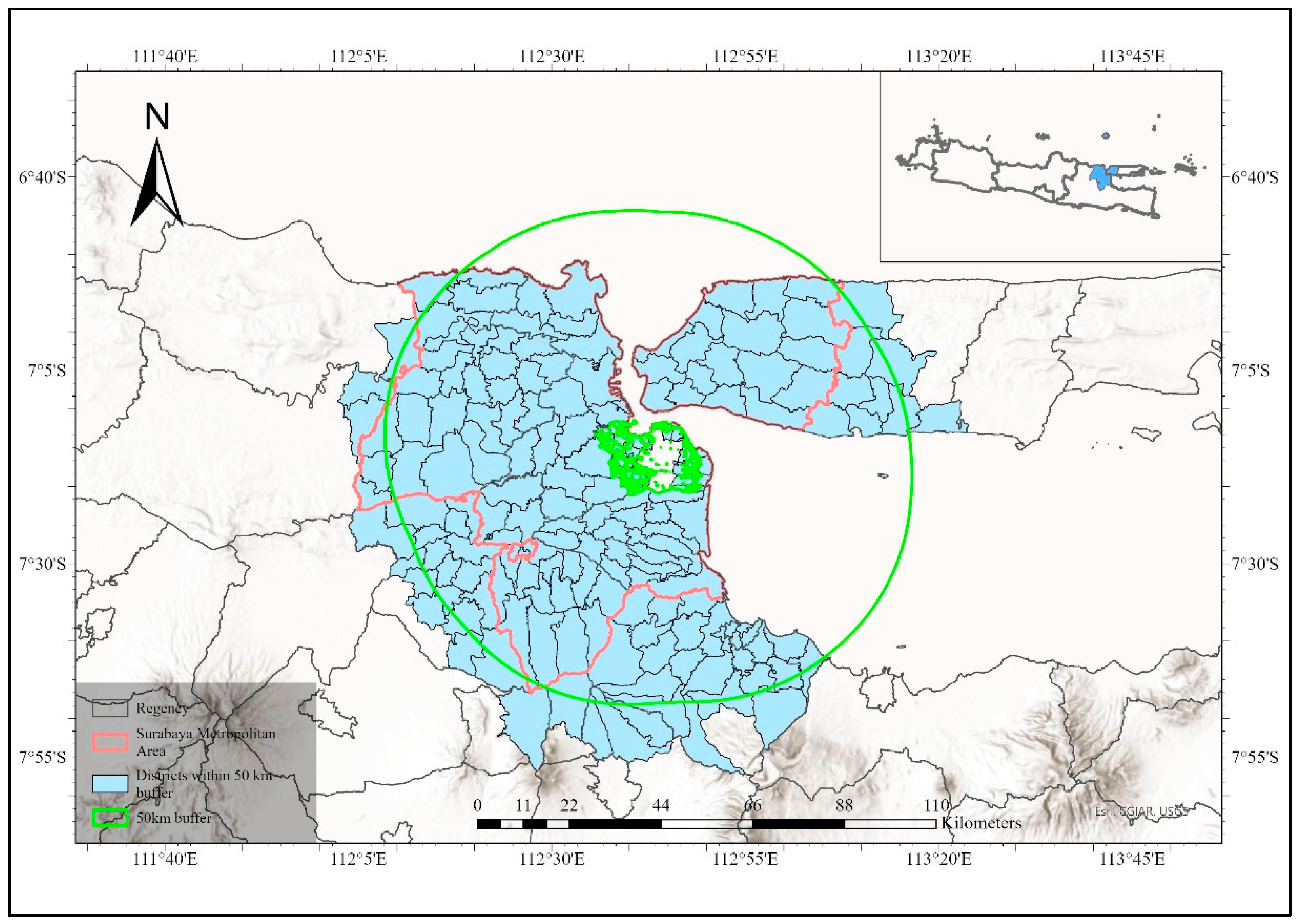
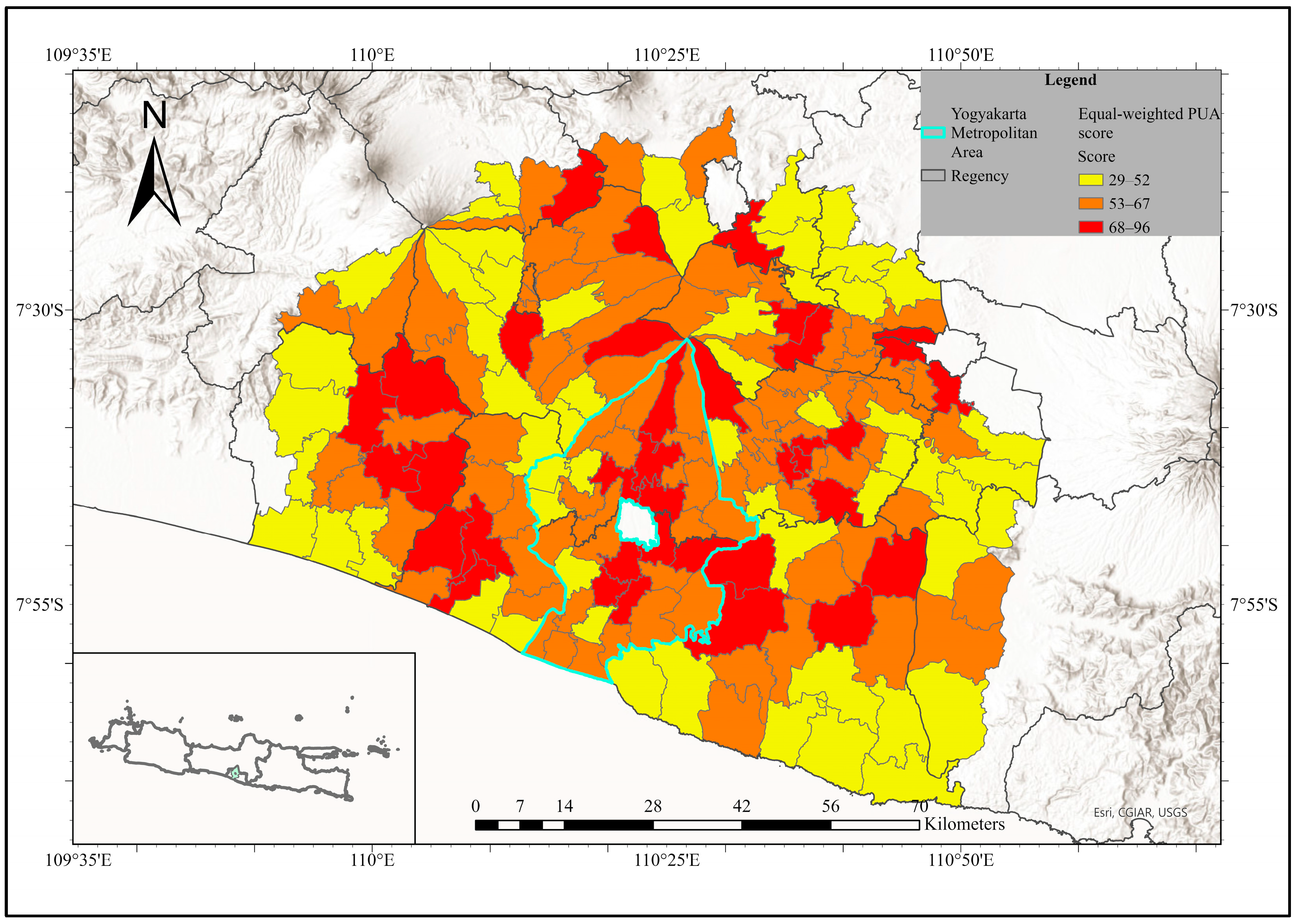
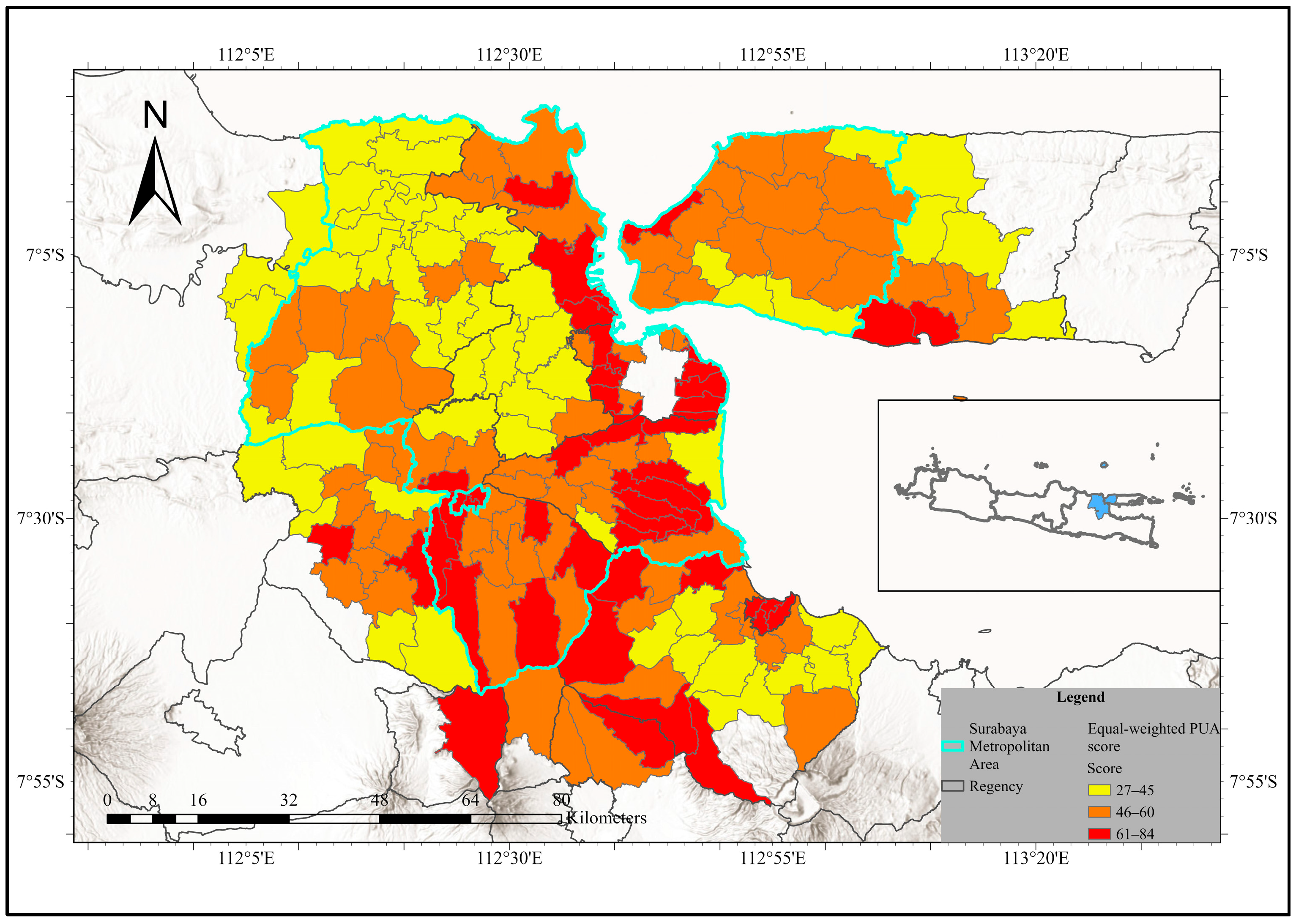
In this study, the delineation of PUAs in the Indonesian cities of Jakarta, Bandung, Yogyakarta, and Surabaya has been meticulously illustrated in Figure 6, Figure 7, and Figure 8, respectively. These areas were systematically identified through a buffering analysis, which employed the urban landscape boundaries of the cities as central points. This methodological approach facilitated the initial selection of 767 districts as potential PUAs, encompassing regions that lie on the fringes of the urban cores.
Particularly in the case of Jakarta and Bandung, which are geographically proximate, there is a notable overlap in their buffered areas, resulting in a combined total of 416 districts identified as potential PUAs. This overlapping region underscores the interconnected nature of the peri-urban zones between these two cities. Within this aggregate, a subset of 181 districts falls outside the metropolitan boundaries of Jakarta and Bandung, highlighting a distinct spatial distribution that warrants separate consideration. Conversely, due to the geographical separation between Surabaya and Yogyakarta, there is no overlap in their respective PUAs. This has resulted in distinct peri-urban boundaries for each city, encompassing 175 districts near Surabaya and 176 districts near Yogyakarta. These findings indicate a clear demarcation of peri-urban extents relative to each urban center, emphasizing the unique spatial dynamics at play.

3.2. Comparison of PUA Delineation from the Equal-Weighted Model and AHP-Weighted Model in Jakarta and Bandung

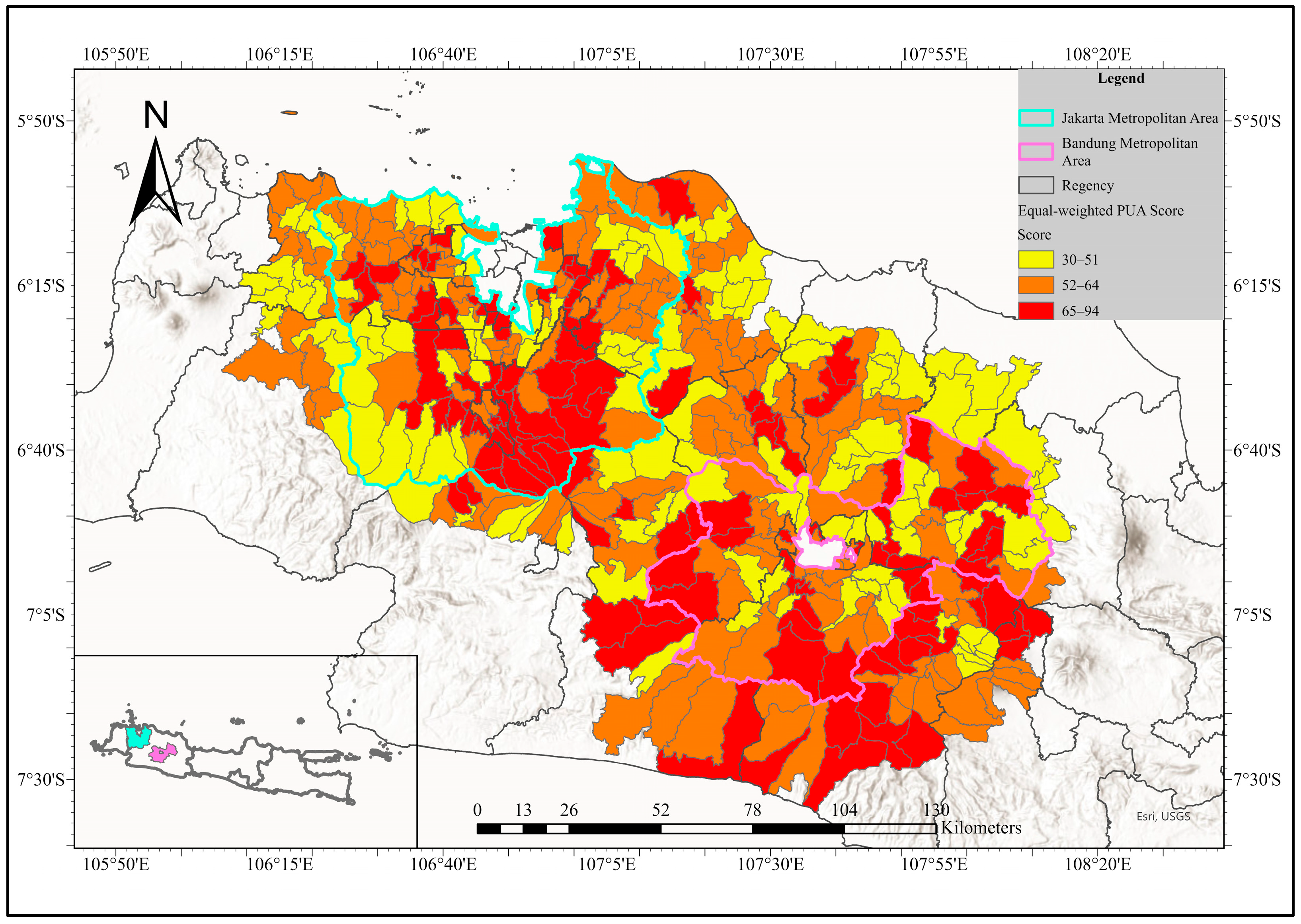
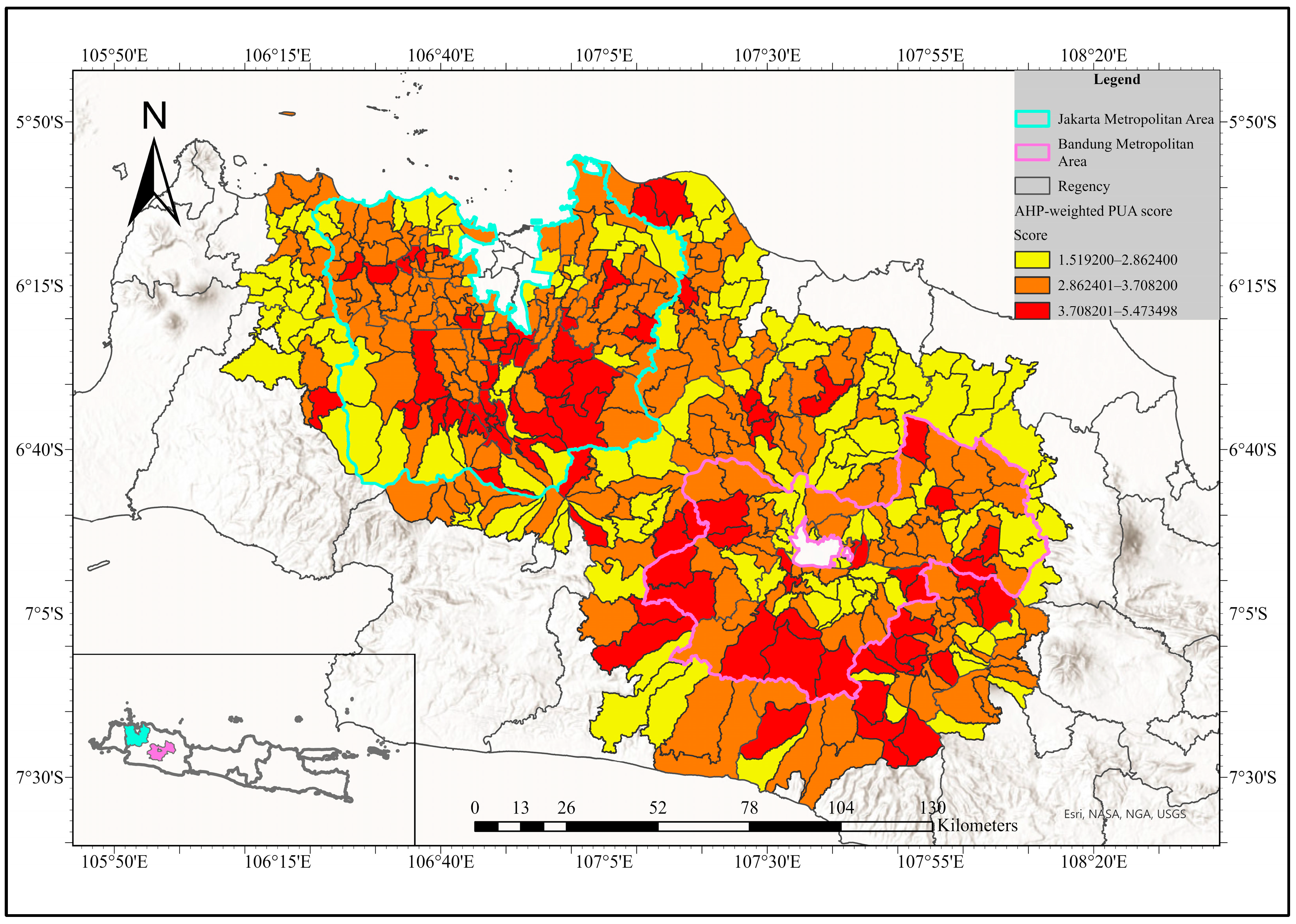
The equal-weighted and AHP-weighted models produced broadly consistent spatial gradients of PUAs across West Java, yet their local delineations exhibited marked differences (Figure 9 and Figure 10). Before comparing the spatial outputs, it should be noted that the numerical scales of the two models differ and are not directly comparable. The equal-weighted model produces composite scores as the arithmetic sum of 18 indicators, each scored on a 1–10 scale, yielding a theoretical range of 18–180. The AHP-weighted model, by contrast, computes scores as a weighted sum in which all weights sum to 1, yielding a theoretical range of 1–10. Despite these scale differences, both sets of scores were classified into three ordinal categories (high, medium, and low) using the Jenks Natural Breaks method, which identifies class boundaries by minimizing within-class variance. This classification enables meaningful categorical and spatial comparison between the two models regardless of their underlying score magnitudes. The equal-weighted model generated more contiguous clusters of high PUA scores, particularly around the peripheries of the Jakarta Metropolitan Area and along the southern margins of Bandung. In contrast, the AHP-weighted model yielded greater spatial fragmentation, with high scores distributed in smaller and more scattered patches.
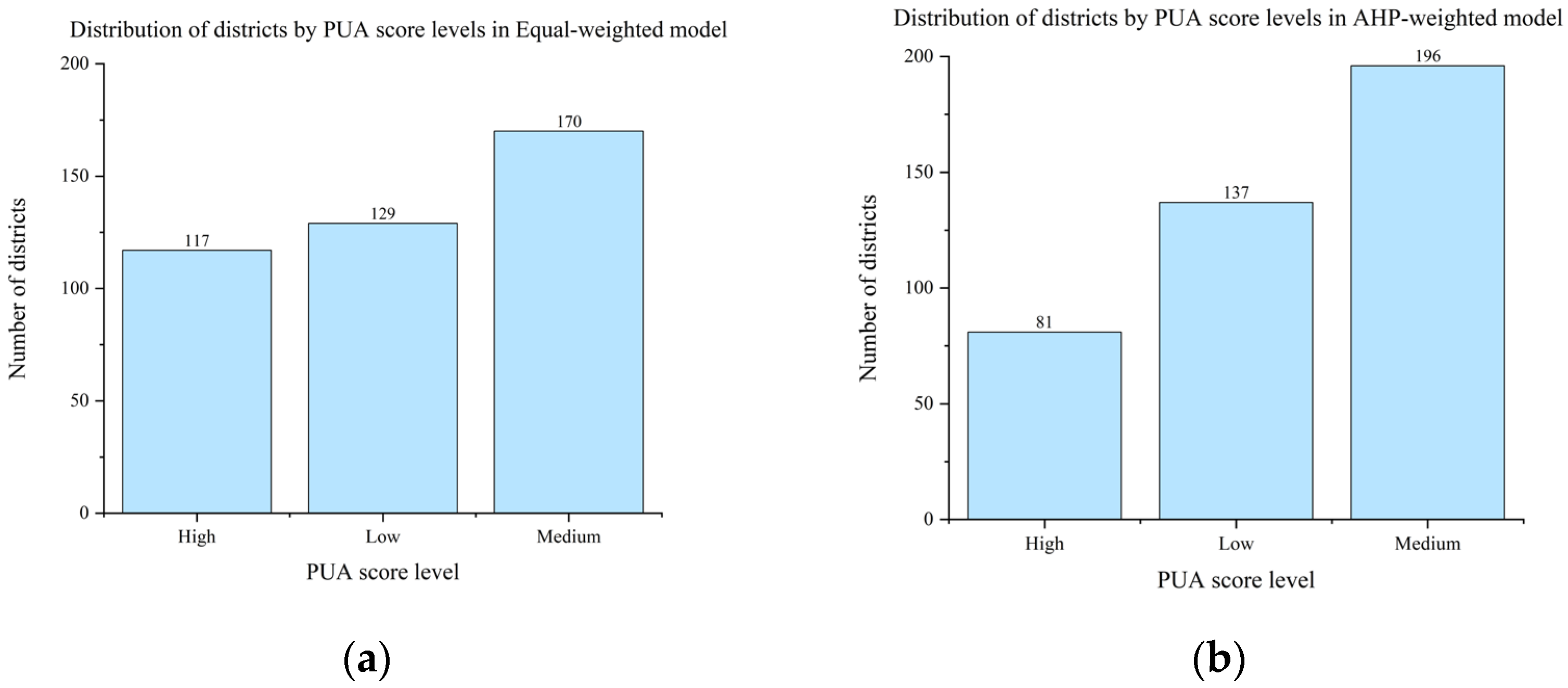
To enable a systematic comparison, continuous PUA scores were reclassified into three ordinal categories—high, medium, and low—corresponding to the red, orange, and yellow ranges in Figure 11. This categorical representation revealed notable shifts in district-level distributions between the two models. The equal-weighted model classified 117 districts as high, 170 as medium, and 129 as low, resulting in a relatively expansive delineation of peri-urban zones. By contrast, the AHP-weighted model reduced the number of high-scoring districts to 81, while increasing the counts of medium and low categories to 196 and 137, respectively. These shifts suggest that the introduction of expert-derived weights moderates the influence of dominant indicators, thereby reducing the extent of high PUA classifications and concentrating more districts in the medium range.
The robustness of the two models was further assessed against expert-based reference scores using Pearson’s r and Spearman’s ρ (Table 2). The equal-weighted model showed moderate and statistically significant correlations with expert assessments across all three metrics (Pearson’s r = 0.517, p = 0.008; Spearman’s ρ = 0.522, p = 0.008; Kendall’s τ = 0.387, p = 0.008), indicating meaningful agreement between the model outputs and expert judgment. By contrast, the AHP-weighted model exhibited weaker and non-significant correlations for Pearson’s r and Spearman’s ρ (Pearson’s r = 0.343, p = 0.094; Spearman’s ρ = 0.389, p = 0.055; Kendall’s τ = 0.284, p = 0.047). The moderate level of agreement observed for the equal-weighted model is consistent with the expected outcome when comparing two genuinely independent assessment systems—a model derived from remote sensing and GIS data versus subjective expert judgment—given the inherent variability in expert assessments and the spatial complexity of peri-urban transitions. Taken together, these findings indicate that the equal-weighted model provides a more reliable approximation of peri-urban characteristics than the AHP-weighted model in this study context.
To quantify the spatial agreement between the two models, a cross-tabulation analysis was conducted across all 416 districts within the 50 km buffer zones of Jakarta and Bandung (Table 3). The overall classification agreement was 65.1% (271 out of 416 districts), with a Cohen’s Kappa of 0.46, indicating moderate agreement. Among districts classified as high by the equal-weighted model, only 53.0% (62 out of 117) were also classified as high by the AHP-weighted model, while 36.8% were downgraded to medium and 10.3% to low. In contrast, medium and low categories showed higher consistency, with approximately 69% and 71% agreement respectively. These results indicate that the two models diverge most in identifying the most peri-urban districts.
To investigate the underlying rationale for the superior performance of the equal-weighted model over the AHP-weighted model, a comparative analysis was conducted between the cross-city variability of the 18 indicators and their respective expert-assigned weights (Table 4). The results reveal distinct indicator profiles across the four cities, reflecting their diverse socio-spatial contexts. Jakarta, as a primary megacity, records the highest mean scores for Population Density (PDB = 3.41), Night Light Intensity (NLI = 4.27), and Population Growth (PGG = 2.66). In contrast, Yogyakarta exhibits a compact yet vegetated form, with peak values in built-up area proportion (PBU = 4.44) and Green Vegetation Fraction (GVF = 8.56). Bandung’s profile is characterized by its mountainous setting, showing the highest scores for forest proportion (PFA = 3.43) and Distance to Forest (DTF = 3.59), while Surabaya maintains a more moderate and balanced profile across most dimensions. Beyond these individual profiles, a significant structural tension is observed between indicator variability and weighting. Ten out of the 18 indicators exhibit cross-city standard deviations (SD) greater than 0.50, indicating high contextual heterogeneity. Notably, several indicators prioritized by expert judgment (AHP weights ≥ 0.08) also display the highest degree of variance, such as Population Density (PDB; SD = 0.71, weight = 0.08) and Population Growth (PGG; SD = 0.58, weight = 0.08). These quantitative findings provide the empirical basis for evaluating the relative robustness of the two weighting schemes.
To further assess the robustness of the equal-weighted model and examine potential indicator redundancy, a leave-one-out sensitivity analysis was conducted. Since the equal-weighted model outperformed the AHP-weighted model, the analysis was performed exclusively on this model. Each of the 18 indicators was sequentially removed, and the model was recalculated using the remaining 17 indicators. The resulting PUA scores were re-validated against expert Q-scores using Pearson’s r, Spearman’s ρ, and Kendall’s τ (Table A2). The results show that the model is robust to the removal of any single indicator, with Pearson’s r remaining within the range of 0.463–0.556 across all 18 iterations. The indicators whose removal caused the largest decline in agreement were PCR (Δr = −0.055), GVF (Δr = −0.054), and PBU (Δr = −0.042), highlighting the central role of land cover composition in capturing peri-urban characteristics. The removal of a smaller number of indicators, such as NEI (Δr = +0.039) and LRD (Δr = +0.025), led to marginal increases in correlation. Rather than indicating redundancy, this suggests that some indicators play a more nuanced or context-dependent role in the model, contributing to the representation of specific dimensions of peri-urban systems that may not be fully captured by dominant variables. Overall, the narrow range of Pearson’s r values across all iterations confirms that the 18-indicator framework is stable and that no single indicator disproportionately drives or undermines model performance.
At the metropolitan scale, the two models diverged in their delineation of peri-urban zones surrounding Jakarta and Bandung. Around Jakarta, the equal-weighted model identified an extensive peri-urban belt that was more consistent with expert-based validation. In contrast, the AHP-weighted model produced narrower and more fragmented PUAs. In Bandung, both models delineated peri-urban zones with similar overall extents, but the AHP-weighted model tended to classify a larger share of districts as medium rather than high. These variations underscore the context-dependent performance of the models, shaped by the distinct land use dynamics of each metropolitan region.
Overall, the results demonstrate that although both models captured the broad spatial gradients of peri-urbanization, the equal-weighted model showed greater agreement with expert validation and thus represents the more robust approach in this case. These differences highlight the context-dependent performance of equal- and AHP-weighted models, which is further elaborated on in the Discussion.

3.3. Spatial Morphology of PUAs

Given that the equal-weighted model outperformed the AHP-weighted model in validation, we used the equal-weighted model as the primary framework for delineating PUAs across the four metropolitan cities (Jakarta, Surabaya, Bandung, and Yogyakarta). The resulting PUA maps displayed coherent spatial patterns that aligned well with the known urban–rural gradients and development histories of each city, indicating that the model performs consistently across settings with different scales, topographies, economic structures, and planning regimes.
Jakarta exhibits a pronounced finger-like sprawl radiating along major transportation corridors toward Bogor, Depok, Tangerang, and Bekasi. This form reflects the combined effects of megacity scale, extreme population density (>15,000 persons/km2), and industrial decentralization policies since the 1970s, which concentrated residential and industrial activities along toll roads and railways [29,61]. The resulting elongated corridors facilitate long-distance commuting while reinforcing polycentric urban structures in the JABODETABEK mega-urban region, consistent with theoretical models of corridor urbanization in Asian megacities [5].
Bandung demonstrates a leapfrog development pattern characterized by scattered, non-contiguous peri-urban patches separated by agricultural land. This fragmented morphology is strongly conditioned by the basin topography, which channels expansion along valley floors while leaving steep slopes undeveloped [30]. Speculative land development has further reinforced discontinuous growth, producing a spatial form that contrasts with Jakarta’s linear peri-urban corridors [29,62].
Yogyakarta presents a more concentric and compact peri-urban belt surrounding the historical urban core (Figure 12). Its morphology reflects a smaller metropolitan scale, moderate population density, and cultural preservation policies that constrain sprawl while sustaining stable agricultural land tenure systems [63,64]. Growth is primarily accommodated through infill and gradual peripheral expansion, aligning with models of bounded urbanization in secondary cities [65].
Surabaya, in contrast, exhibits large, consolidated peri-urban agglomerations concentrated in the southern and southwestern directions (Figure 13). This morphology is driven by the city’s industrial and port-oriented development strategy, which has promoted coordinated expansion along the Brantas River delta and toward Gresik [63,66]. The continuity of these peri-urban clusters highlights the decisive role of state-led industrial policy and infrastructure investment in shaping metropolitan form, producing planned agglomerations rather than fragmented sprawl [66].
Taken together, these patterns underscore the context-dependent nature of peri-urbanization in Java and Southeast Asia [36,63]. Jakarta’s radial corridors illustrate the outward pressures of megacity scale and transport-enabled commuting [67,68], while Bandung’s leapfrog expansion emphasizes the interaction between topographic constraints and fragmented land markets [3,35]. Yogyakarta’s compact morphology reflects how cultural institutions and smaller urban scale constrain sprawl [69], whereas Surabaya demonstrates the formative power of state intervention and industrial policy in creating large-scale peri-urban agglomerations [66,70].
Overall, the morphological diversity observed across these metropolitan regions confirms that peri-urbanization in Southeast Asia follows multiple trajectories rather than a singular model. Urban scale, economic development stage, transportation infrastructure, and historical planning interventions jointly produce distinct forms of urban–rural transitions [71]. These findings challenge universal models of peri-urban growth and highlight the need for context-sensitive approaches in both analytical frameworks and planning interventions [72,73].

4. Discussion

This study provides three major insights into the delineation of peri-urban areas using indicator-based frameworks. First, the equal-weighted model consistently outperformed the AHP-weighted model, demonstrating that subjective expert-derived weights do not necessarily enhance—and may even diminish—the accuracy of peri-urban identification in heterogeneous metropolitan environments. Second, the multi-dimensional indicator framework proved effective in capturing the socioeconomic, infrastructural, and functional gradients that characterize peri-urban transitions across Java, underscoring the value of integrating non-physical dimensions into PUA delineation. Third, the expert scoring (Q-score) validation framework offered a practical and transparent means of assessing delineation quality in the absence of a universal ground truth, confirming the robustness of indicator-based methods for guiding planning and land use assessments.

4.1. AHP-Weighted Model and Equal-Weighted Model Performance

The statistically significant performance of the equal-weighted model over the questionnaire-weighted approach represents a significant methodological finding that challenges prevailing assumptions regarding expert knowledge integration in spatial modeling frameworks [74]. This counterintuitive outcome reveals fundamental limitations inherent in subjective weighting schemes that can compromise model reliability and spatial accuracy in complex urban systems.
The AHP-weighted model’s underperformance can be attributed to three interconnected theoretical issues. First, expert assessments inevitably introduce cognitive biases and disciplinary perspectives that may not align with the empirical spatial processes governing peri-urban development [75]. The heterogeneity of professional backgrounds, spanning urban planning, geography, remote sensing, and policy sectors, creates inconsistencies in weight assignments that reflect theoretical priorities rather than empirical realities of urban fringe dynamics [75,76].
Second, our findings (in Section 3.2) suggest that the poor performance of the AHP-weighted model stems from a sensitivity to inter-city variance. In the AHP framework, expert judgment assigned high priority (weight = 0.08) to dimensions such as Population Density (PDB) and Population Growth (PGG). However, these indicators also exhibited the highest spatial volatility across the four study cities (SD = 0.71 and 0.58, respectively). By applying a heavy, uniform weight to indicators that vary by more than a factor of two between cities (e.g., Jakarta vs. Yogyakarta), the AHP model introduces a compounding bias.
Third, the equal-weighted approach demonstrates superior performance by preserving the intrinsic variance–covariance structures within the indicator dataset without imposing predetermined hierarchies [77]. This data-driven flexibility proves particularly valuable in complex, multi-factorial systems where indicator interactions exhibit non-linear and context-dependent characteristics [78]. The statistically significant validation outcomes confirm that empirical signals within comprehensive indicator datasets contain sufficient information for meaningful peri-urban delineation without requiring subjective weight adjustments.
It should be noted, however, that the superior performance of the equal-weighted model in this study is grounded in the specific socio-spatial context of Java’s metropolitan regions. These environments are characterized by high contextual heterogeneity, evidenced by 10 of the 18 indicators displaying cross-city standard deviations (SD) exceeding 0.50 (Table 4). The equal-weighted model provides a “smoothing effect” that mitigates the influence of extreme local outliers. This finding does not suggest that equal weighting is a universal replacement for expert-based approaches like AHP. Rather, it highlights a trade-off: while AHP may offer higher precision in single-city studies or homogeneous urban systems where expert priors are stable, equal weighting offers greater methodological robustness in multi-city comparative frameworks. In diverse landscapes where peri-urbanization is driven by a shifting mix of infrastructure, agriculture, and demographics, a non-hierarchical weighting scheme prevents the model from becoming overly sensitive to the fluctuations of a single dominant variable.

4.2. Methodological Contribution

Beyond the superiority of equal weighting, the study highlights the methodological advantages of the multi-dimensional indicator-based framework. Compared to remote sensing index approaches, which typically rely on spectral characteristics such as NDVI gradients, normalized built-up indices, or landscape metrics [79], our methodology integrates socioeconomic dimensions that capture functional and behavioral aspects of peri-urban transitions [80]. Remote sensing indices, while valuable for detecting physical landscape transformations, often fail to represent the complex socioeconomic processes that define PUAs in Southeast Asian contexts [80]. Java Island’s intensive agricultural systems, mixed-use developments, and traditional settlement patterns generate spectral signatures that confound purely physical classification approaches, leading to misclassification of transitional landscapes [3]. Our integration of economic activity diversity indicators, infrastructure accessibility measures, and social condition variables provides a more nuanced representation of the gradual urban–rural continuum characteristic of Indonesian metropolitan fringes. Unlike density gradient methods, which assume monotonic distance–decay relationships from urban cores to rural peripheries, our approach accommodates the discontinuous and heterogeneous spatial patterns common in rapidly urbanizing regions [38]. Traditional density gradient models often fail to capture leapfrog development, scattered industrial zones, and mixed land uses that characterize contemporary peri-urban landscapes [3]. Our methodology explicitly incorporates spatial discontinuities and functional heterogeneity, avoiding the analytical limitations inherent in linear distance-based models. Census clustering approaches, while incorporating demographic variables, typically lack the spatial resolution and multi-dimensional scope necessary for precise peri-urban boundary delineation [81]. These methods often suffer from modifiable areal unit problems and temporal lags in data availability that limit their applicability for dynamic peri-urban analysis [82]. By integrating remote sensing-derived spatial indicators with sub-district-level socioeconomic data, our methodology provides enhanced spatial precision while maintaining sensitivity to functional characteristics of urban fringe areas.
The theoretical contribution of this framework lies in its synthesis of multiple analytical traditions into a unified methodology. By simultaneously incorporating physical, socioeconomic, and accessibility indicators, the approach transcends disciplinary silos while retaining analytical rigor [74,83]. The systematic validation against expert reference scores ensures interpretability within urban planning and policy contexts, while the statistically significant performance of the equal-weighted scheme across diverse metropolitan environments demonstrates the method’s robustness and transferability [84]. Importantly, this approach advances ongoing debates around the integration of big data and traditional spatial analysis, showing that comprehensive indicator integration can yield reliable and transparent results without complex weighting schemes. Collectively, these findings establish the indicator-based framework as a robust and generalizable methodology for peri-urban analysis, addressing the limitations of existing approaches while offering practical utility for comparative urban research and planning applications across heterogeneous metropolitan contexts.

4.3. Limitations and Future Research Directions

Like any empirical study, this research faces limitations that also reflect the inherent challenges of peri-urban analysis. Validation relied on expert-based reference scores, which, while subjective, represent one of the most widely accepted benchmarks in peri-urban studies where universally observable ground truth does not exist [71,73,85]. These reference scores (Q-scores) were derived from qualitative survey responses that capture stakeholder perceptions of district-level characteristics, rather than direct evaluation of the spatial indicators used in the models, thereby providing an alternative perception-based benchmark for comparison. While this approach reduces direct circularity, the Q-score does not constitute a fully independent empirical validation dataset. Nevertheless, it offers a practical and context-sensitive reference in the absence of universally observable ground-truth data for peri-urban delineation.
Potential bias was reduced by retaining only logically consistent responses (CR < 0.1), and the statistically significant alignment of the equal-weighted model with these references demonstrates their value as a meaningful benchmark. The expert survey sample, although systematically designed, was limited to 80 respondents, predominantly academics and planners; this ensured decision-making expertise but may not fully represent community perspectives [40]. The geographic scope, restricted to four cities on Java Island, constrains external validity, yet focusing on Indonesia’s demographic and economic core strengthens internal comparability [86]. Finally, the cross-sectional design offers a static snapshot rather than capturing temporal trajectories, but it establishes a robust baseline for comparative analysis across metropolitan contexts [87].
Although the leave-one-out sensitivity analysis confirmed the robustness of the 18-indicator framework (Table A2), future research could employ more comprehensive techniques such as principal component analysis (PCA) or variance inflation factor (VIF) analysis to evaluate inter-indicator correlations prior to model construction, and explore data-driven variable selection methods to further optimize the indicator system.
Building on these limitations, future research should refine weight allocation through hybrid approaches that integrate expert judgment with data-driven optimization techniques such as genetic algorithms, neural networks, or particle swarm methods [88]. Additionally, systematic sensitivity analyses of weighting schemes—such as varying AHP weights within confidence intervals, testing alternative weighting methods (e.g., entropy weighting), or employing Monte Carlo simulations of weight perturbations—could further clarify the conditions under which differential weighting outperforms equal weighting [78,79]. Validation frameworks need to be strengthened by triangulating expert assessments with high-resolution remote sensing, socioeconomic data, and participatory mapping to create multi-perspective benchmarks [89,90]. Extending the framework beyond Java to other Indonesian islands and cross-national cases will test transferability and reveal universal versus context-specific drivers of peri-urbanization [72,91]. Future studies could explore adaptive, city-specific boundary approaches—such as those based on commuting sheds, transport network accessibility, or topographic constraints—to replace the uniform buffer distance used in this study, potentially improving the precision of the initial scoping step for cities with distinct physical geographies. Finally, adopting time-series perspectives and advanced methods such as convolutional neural networks applied to multi-temporal datasets could transform static delineations into predictive models, while real-time monitoring systems that combine satellite imagery, mobile phone data, and economic indicators would provide adaptive insights for managing rapidly evolving peri-urban transitions [92,93].

5. Conclusions

This study developed an indicator-based framework to delineate PUAs in four major cities in Java, and it showed that the equal-weighted model outperformed the AHP-weighted approach in validation. The findings highlight that data-driven weighting better captures the complex interactions among socioeconomic, infrastructural, and spatial indicators, while expert-derived weights may introduce biases that reduce accuracy. Distinct spatial morphologies were identified, such as Jakarta’s corridor-like expansion and Yogyakarta’s compact concentric form, reflecting the diverse trajectories of peri-urbanization shaped by geography, infrastructure, and planning legacies. Methodologically, the study advances peri-urban analysis by integrating multi-dimensional indicators into a unified framework, and, practically, provides a transparent and transferable tool for planning and policymaking. Although the analysis was limited to four cities in Java and relied on expert-based validation, future research should extend the framework geographically, incorporate multi-temporal data, and explore hybrid approaches that combine expert knowledge with machine-learning optimization to enhance predictive capacity.

Author Contributions

Conceptualization, Z.W. and A.M.K.; methodology, Z.W.; software, Z.W.; validation, Z.W. and A.M.K.; formal analysis, Z.W.; investigation, Z.W.; resources, B.S.W.; data curation, Z.W.; writing—original draft preparation, Z.W.; writing—review and editing, Z.W., A.M.K., M.A.A. and A.A.A.; visualization, Z.W.; supervision, A.M.K., M.A.A., A.A.A. and B.S.W.; project administration, A.A.A.; funding acquisition, A.A.A. All authors have read and agreed to the published version of the manuscript.

Funding

This research was funded by the Department of Foreign Affairs and Trade (DFAT) Australia through KONEKSI (Australia-Indonesia Knowledge Partnerships Platform). The project was conducted under the title “Addressing vulnerabilities and enhancing resilience in the smallholder value chains of Java’s peri-urban food supply systems”, with grant number 1447/CRG/2023/28-UQ. The views expressed in this publication are the authors’ alone and are not necessarily the views of the Australian Government.

Data Availability Statement

The data presented in this study are available on request from the corresponding author.

Acknowledgments

The authors would like to express their sincere gratitude to the experts and practitioners who participated in the survey and shared their valuable insights, which greatly contributed to this study. The authors also gratefully acknowledge the significant contributions of Ike Sari Astuti from Universitas Negeri Malang, whose expertise and active involvement in the research design and data analysis were instrumental in shaping this work.

Conflicts of Interest

The authors declare no conflicts of interest.

Appendix A

Table A1. The 18 Indicators used for mapping PUAs.
Indicator CategoriesIndicatorsDescriptionFormulaData Source of the VariableReference
Land Cover/Land Cover Change (LULC)Proportion of Build-up Area (PBU) %Measures the proportion of land occupied by built-up structures in each district. (BUA/ARE) × 100%BIG 1[21,44,51]
BUA = built-up area (ha); ARE = district area (ha)
Proportion of Crop Area (PCR) %Measures the proportion of land under crop cultivation, reflecting agricultural activity. (CRO/ARE) × 100%BIG[53]
CRO = crop area (ha); ARE = district area (ha)
Build-up Growth Rate during 2010 to 2020 (BGG) %Captures the rate of built-up area expansion over a decade, indicating urbanization dynamics. (BUG_2020-BUG_2010)/BUG_2010 × 100%GHSL 2[51]
BUG_2020 = built-up area from GHSL in 2020 (ha); BUG_2010 = built-up area from GHSL in 2010 (ha)
Proportion of Green Vegetation Fraction(GVF) %Measures the proportion of pixel area occupied by green vegetation, reflecting the ecological condition of each district.Proportion of pixel occupied by vegetationFraction of Vegetation Cover (FCover) product from the Copernicus Global Land Service website[53]
Proportion of Impervious Surface Fraction (ISF) %Measures the proportion of pixel area occupied by impervious surfaces including roads, parking lots, and other sealed non-building features.Proportion of pixel occupied by vegetationGHS-BUILT-S R2023A dataset from the GHSL[53]
Proportion of Forest Area (PFA) %Measures the proportion of land covered by forest, indicating the degree of natural landscape preservation. (FOR/ARE) × 100%BIG[21]
FOR = forest area (ha); ARE = district area (ha)
Economic Factor (EF)Number of Economic Resources per area (NEI) /haReflects the economic activity intensity by measuring the density of economic resources (banks, ATMs, markets) per unit area.Number of Economic Resources/AREBIG[43]
Night Light Intensity in 2020 (NLI)Captures nighttime economic activity and urbanization intensity through satellite-derived nighttime light radiance values.Mean value of satellite night time pixels in each district from VIRSNOAA VIIRS DNB ANNUAL V2.1 dataset on Google Earth Engine[44,46]
Demographic Factor (DF)Population Density (PDB) P/Km2Measures population concentration per unit area, a fundamental indicator of urbanization level. POP/ARE × 100%BPS 3[21,43,44,45,46]
POP = total population; ARE = district area (ha)
Population Growth Rate from 2010 to 2020 (PGG) %Captures population change over a decade, reflecting demographic dynamics associated with peri-urban growth. (POG_2020-POG_2010)/POG_2010 × 100%The GHS-POP R2023A dataset of the GHSL[45,46,51,53]
POG_2020 = population from GHSL in 2020; POG_2010 = population from GHSL in 2010
Arterial Road Density (ART) km/haMeasures the density of major arterial roads, reflecting higher-level transport infrastructure. LART/ARE
LART = total length of arterial roads (km); ARE = district area (ha)BIG[43]
Infrastructural Factor (IF)Collector Road Density (CRD) Km/haMeasures the density of collector roads that link arterial and local roads. COL/AREBIG[43]
LCOL = total length of collector roads (km); ARE = district area (ha)
Local Road Density (LRD) Km/haMeasures the density of local roads serving residential and community access. LOC/AREBIG[43]
LOC = total length of local roads (km); ARE = district area (ha)
Number of Public Facilities per area (NFP)/haMeasures the density of public facilities (schools, hospitals, government offices) per unit area, indicating service provision level.SHP points of public facilities collected from OSM dataOSM 4 [53]
Spatial Accessibility (SA) Distance to City Center (DTC) kmMeasures the average travel distance from each district to the nearest city center, reflecting spatial accessibility to urban services.Average distance pixel values in each district to the city center, cost layer GIS, calculated from the road SHP layerBIG[52]
Distance to Forest (DTF) kmMeasures the average distance from each district to the nearest forest area, reflecting proximity to natural landscapes.Average pixel values of the distance to the forestBIG[50]
Landscape Structural (LS)Built-up Area Patches Density in each district (BPD) Measures the number of discrete built-up patches per unit area, reflecting urban sprawl and discontinuous development patterns. NPB/AREBIG[50]
NPB = number of built-up patches; ARE = district area (ha)
Patch Density (PDN)Measures the total number of landscape patches per unit area, reflecting overall landscape fragmentation. N/AREBIG[53]
N = total number of patches; ARE = district area (ha)
1 BIG means Geospatial Information Agency of Indonesia (Badan Informasi Geospasial). 2 GHSL means Global Human Settlement Layer. 3 Badan Pusat Statistik. 4 OpenStreetMap.
Table A2. Leave-one-out sensitivity analysis of the equal-weighted model.
Removed IndicatorDimension 1Pearson’s rΔrSpearman’s ρΔρKendall’s τΔτ
None (Baseline)0.51730.52090.3852
PBULULC0.4758−0.04150.4300−0.09090.3272−0.0580
PCRLULC0.4627−0.05460.4616−0.05930.3486−0.0366
BGGLULC0.5133−0.00400.5234+0.00250.3731−0.0120
GVFLULC0.4629−0.05440.4497−0.07120.3059−0.0793
ISFLULC0.5369+0.01960.5644+0.04350.4339+0.0488
PFOLULC0.4887−0.02860.4893−0.03160.3581−0.0270
NEIEF0.5562+0.03890.5688+0.04790.4243+0.0391
NLIEF0.5042−0.01310.5159−0.00500.3879+0.0027
PDBDF0.5137−0.00360.5304+0.00950.3960+0.0108
PGGDF0.5068−0.01040.5212+0.00030.3797−0.0055
ARTIF0.5176+0.00030.4954−0.02550.3474−0.0378
CRDIF0.5211+0.00380.5287+0.00780.3892+0.0040
LRDIF0.5420+0.02470.5763+0.05540.4301+0.0450
NFPIF0.5350+0.01770.5701+0.04920.4216+0.0364
DTCSA0.4890−0.02830.4260−0.09490.3277−0.0574
DTFSA0.4873−0.03000.4050−0.11590.3283−0.0569
BPDLS0.5541+0.03680.5563+0.03540.4014+0.0162
PDNLS0.4949−0.02230.4921−0.02880.3716−0.0135
1 LULC = Land Use and Land Cover; EF = Economic Factor; DF = Demographic Factor; IF = Infrastructure Factor; SA = Spatial Accessibility; LS = Landscape Structure; PCR = Proportion of Cropland; GVF = Proportion of Green Vegetation Fraction; PBU = Proportion of Build-up Area; PFA = Proportion of Forest Area; ISF = Proportion of Impervious Surface Fraction; BGG = Build-up Growth Rate during 2010 to 2020; NEI = Number of Economic Resources per area; NLI = Night Light Intensity in 2020; PDB = Population Density; PGG = Population Growth Rate from 2010 to 2020; ART = Arterial Road Density; CRD = Collector Road Density; LRD = Local Road Density; NFP = Number of Public Facilities per area; DTC = Distance to City Center; DTF = Distance to Forest; BPD = Built-up Area Patches Density in each district; PDN = Patch Density.

References

  1. Grimm, N.B.; Faeth, S.H.; Golubiewski, N.E.; Redman, C.L.; Wu, J.; Bai, X.; Briggs, J.M. Global change and the ecology of cities. Science 2008, 319, 756–760. [Google Scholar] [CrossRef] [Scilit]
  2. He, X.; Zhou, C.; Zhang, J.; Yuan, X. Using wavelet transforms to fuse nighttime light data and POI big data to extract urban built-up areas. Remote Sens. 2020, 12, 3887. [Google Scholar] [CrossRef] [Scilit]
  3. Seto, K.C.; Güneralp, B.; Hutyra, L.R. Global forecasts of urban expansion to 2030 and direct impacts on biodiversity and carbon pools. Proc. Natl. Acad. Sci. USA 2012, 109, 16083–16088. [Google Scholar] [CrossRef] [Scilit]
  4. Ahani, S.; Dadashpoor, H. A review of domains, approaches, methods and indicators in peri-urbanization literature. Habitat Int. 2021, 114, 102387. [Google Scholar] [CrossRef] [Scilit]
  5. Zhang, Q.; Seto, K.C. Mapping urbanization dynamics at regional and global scales using multi-temporal DMSP/OLS nighttime light data. Remote Sens. Environ. 2011, 115, 2320–2329. [Google Scholar] [CrossRef] [Scilit]
  6. Peng, J.; Hu, Y.N.; Liu, Y.; Ma, J.; Zhao, S. A new approach for urban-rural fringe identification: Integrating impervious surface area and spatial continuous wavelet transform. Landsc. Urban Plan. 2018, 175, 72–79. [Google Scholar] [CrossRef] [Scilit]
  7. Opitz, I.; Berges, R.; Piorr, A.; Krikser, T. Contributing to food security in urban areas: Differences between urban agriculture and peri-urban agriculture in the Global North. Agric. Hum. Values 2016, 33, 341–358. [Google Scholar] [CrossRef] [Scilit]
  8. Tsuchiya, K.; Hara, Y.; Thaitakoo, D. Linking food and land systems for sustainable peri-urban agriculture in Bangkok Metropolitan Region. Landsc. Urban Plan. 2015, 143, 192–204. [Google Scholar] [CrossRef] [Scilit]
  9. Rizkiya, P.; Fuady, Z.; Mahardika, R.P.; Hasan, Z.; Gunawan, A. The growth of built-up area of Banda Aceh and its implication to agricultural land in peri-urban area in Aceh Besar Regency. In Proceedings of the AIP Conference Proceedings; AIP Publishing LLC: Melville, NY, USA, 2024. [Google Scholar] [CrossRef] [Scilit]
  10. Sahana, M.; Ravetz, J.; Patel, P.P.; Dadashpoor, H.; Follmann, A. Where Is the Peri-Urban? A Systematic Review of Peri-Urban Research and Approaches for Its Identification and Demarcation Worldwide. Remote Sens. 2023, 15, 1316. [Google Scholar] [CrossRef] [Scilit]
  11. Pribadi, D.O.; Pauleit, S. The dynamics of peri-urban agriculture during rapid urbanization of Jabodetabek Metropolitan Area. Land Use Policy 2015, 48, 13–24. [Google Scholar] [CrossRef] [Scilit]
  12. Whitehand, J.W.R. Urban fringe belts: Development of an idea. Plan. Perspect. 1988, 3, 47–58. [Google Scholar] [CrossRef] [Scilit]
  13. Pryor, R.J. Defining the rural-urban fringe. Soc. Forces 1968, 47, 202–215. [Google Scholar] [CrossRef] [Scilit]
  14. Peng, J.; Zhao, S.; Liu, Y.; Tian, L. Identifying the urban-rural fringe using wavelet transform and kernel density estimation: A case study in Beijing City, China. Environ. Model. Softw. 2016, 83, 286–302. [Google Scholar] [CrossRef] [Scilit]
  15. Wang, C.; Sun, X.; Liu, Z.; Xia, L.; Liu, H.; Fang, G.; Liu, Q.; Yang, P. A novel full-resolution convolutional neural network for urban-fringe-rural identification: A case study of urban agglomeration region. Landsc. Urban Plan. 2024, 249, 105122. [Google Scholar] [CrossRef] [Scilit]
  16. Paudel, B.; Gao, J.; Zhang, Y.; Wu, X.; Li, S.; Yan, J. Changes in Cropland Status and Their Driving Factors in the Koshi River Basin of the Central Himalayas, Nepal. Sustainability 2016, 8, 933. [Google Scholar] [CrossRef] [Scilit]
  17. Serra, P.; Pons, X.; Saurí, D. Land-cover and land-use change in a Mediterranean landscape: A spatial analysis of driving forces integrating biophysical and human factors. Appl. Geogr. 2008, 28, 189–209. [Google Scholar] [CrossRef] [Scilit]
  18. Doan, P.; Oduro, C.Y. Patterns of population growth in peri-urban Accra, Ghana. Int. J. Urban Reg. Res. 2012, 36, 1306–1325. [Google Scholar] [CrossRef] [Scilit]
  19. Rogus, S.; Dimitri, C. Agriculture in urban and peri-urban areas in the United States: Highlights from the Census of Agriculture. Renew. Agric. Food Syst. 2015, 30, 64–78. [Google Scholar] [CrossRef] [Scilit]
  20. Susilo, B. Map analysis and spatial statistic: Assessment of spatial variability of agriculture land conversion at urban fringe area of Yogyakarta. In Proceedings of the IOP Conference Series: Earth and Environmental Science; IOP Publishing: Bristol, UK, 2016; p. 012001. [Google Scholar] [CrossRef] [Scilit]
  21. Danielaini, T.T.; Maheshwari, B.; Hagare, D. Defining rural–urban interfaces for understanding ecohydrological processes in West Java, Indonesia: Part I. Development of methodology to delineate peri-urban areas. Ecohydrol. Hydrobiol. 2018, 18, 22–36. [Google Scholar] [CrossRef] [Scilit]
  22. Moreira, F.; Fontes, I.; Dias, S.; e Silva, J.B.; Loupa-Ramos, I. Contrasting static versus dynamic-based typologies of land cover patterns in the Lisbon metropolitan area: Towards a better understanding of peri-urban areas. Appl. Geogr. 2016, 75, 49–59. [Google Scholar] [CrossRef] [Scilit]
  23. Thapa, R.B.; Murayama, Y. Land evaluation for peri-urban agriculture using analytical hierarchical process and geographic information system techniques: A case study of Hanoi. Land Use Policy 2008, 25, 225–239. [Google Scholar] [CrossRef] [Scilit]
  24. Cho, S.-H.; Poudyal, N.; Lambert, D.M. Estimating spatially varying effects of urban growth boundaries on land development and land value. Land Use Policy 2008, 25, 320–329. [Google Scholar] [CrossRef] [Scilit]
  25. Fan, C.S.; Stark, O. Rural-to-urban migration, human capital, and agglomeration. J. Econ. Behav. Organ. 2008, 68, 234–247. [Google Scholar] [CrossRef] [Scilit]
  26. Žlender, V. Characterisation of peri-urban landscape based on the views and attitudes of different actors. Land Use Policy 2021, 101, 105181. [Google Scholar] [CrossRef] [Scilit]
  27. Mulya, S.P.; Hudalah, D.; Prilandita, N. Developing a new methodology for determining typologies of peri-urban agriculture: A case study of the Jakarta Bandung Mega Urban Region Indonesia. Land Use Policy 2024, 146, 107310. [Google Scholar] [CrossRef] [Scilit]
  28. Badan Pusat Statistik. Indonesia Administrative Division Statistics; Statistics Indonesia: Jakarta, Indonesia, 2023.
  29. Firman, T. Major issues in Indonesia’s urban land development. Land Use Policy 2004, 21, 347–355. [Google Scholar] [CrossRef] [Scilit]
  30. Hudalah, D.; Winarso, H.; Woltjer, J. Peri-urbanisation in East Asia: A new challenge for planning? Int. Dev. Plan. Rev. 2007, 29, 503–519. [Google Scholar] [CrossRef] [Scilit]
  31. Firman, T. The continuity and change in mega-urbanization in Indonesia: A survey of Jakarta–Bandung Region (JBR) development. Habitat Int. 2009, 33, 327–339. [Google Scholar] [CrossRef] [Scilit]
  32. Government of Indonesia. Master Plan for the Acceleration and Expansion of Indonesia’s Economic Development 2011–2025 (MP3EI); Coordinating Ministry for Economic Affairs: Jakarta, Indonesia, 2011.
  33. Ministry of Home Affairs of the Republic of Indonesia. Regulation on Administrative Regions and Boundaries; Ministry of Home Affairs of the Republic of Indonesia: Jakarta, Indonesia, 2022.
  34. Dangalle, N.; Närman, A. Peri-urban development in Gampaha district, Sri Lanka. In The Peri-Urban Interface; Routledge: Abingdon-on-Thames, UK, 2012; pp. 186–201. [Google Scholar]
  35. Webster, D.R.; Cai, J.; Muller, L.; Luo, B. Peri-Urbanization in Chengdu, Western China: From “Third Line” to Market Dynamics; Asia-Pacific Research Center, Stanford University: Stanford, CA, USA, 2004; Available online: https://fsi9-prod.s3.us-west-1.amazonaws.com/s3fs-public/Webster_etal_Chengdu_2004.pdf (accessed on 27 March 2026).
  36. McGee, T.G. The Southeast Asian city: A Social Geography of the Primate Cities of Southeast Asia. 1967. Available online: https://archive.org/details/southeastasianci0000mcge/page/n237/mode/2up (accessed on 27 March 2026).
  37. Kontgis, C.; Schneider, A.; Fox, J.; Saksena, S.; Spencer, J.H.; Castrence, M. Monitoring peri-urbanization in the greater Ho Chi Minh City metropolitan area. Appl. Geogr. 2014, 53, 377–388. [Google Scholar] [CrossRef] [Scilit]
  38. Tian, L.; Ge, B.; Li, Y. Impacts of state-led and bottom-up urbanization on land use change in the peri-urban areas of Shanghai: Planned growth or uncontrolled sprawl? Cities 2017, 60, 476–486. [Google Scholar] [CrossRef] [Scilit]
  39. Amoateng, P.; Cobbinah, P.B.; Owusu-Adade, K. Managing physical development in peri-urban areas of Kumasi, Ghana: A case of Abuakwa. J. Urban Environ. Eng. 2013, 7, 96–109. [Google Scholar] [CrossRef] [Scilit]
  40. Cobbinah, P.B.; Gaisie, E.; Owusu-Amponsah, L. Peri-urban morphology and indigenous livelihoods in Ghana. Habitat Int. 2015, 50, 120–129. [Google Scholar] [CrossRef] [Scilit]
  41. Liu, Z.; Robinson, G.M. Residential development in the peri-urban fringe: The example of Adelaide, South Australia. Land Use Policy 2016, 57, 179–192. [Google Scholar] [CrossRef] [Scilit]
  42. Shi, Y.; Sun, X.; Zhu, X.; Li, Y.; Mei, L. Characterizing growth types and analyzing growth density distribution in response to urban growth patterns in peri-urban areas of Lianyungang City. Landsc. Urban Plan. 2012, 105, 425–433. [Google Scholar] [CrossRef] [Scilit]
  43. Fang, L.; Wang, Y. Multi-Disciplinary Determination of the Rural/Urban Boundary: A Case Study in Xi’an, China. Sustainability 2018, 10, 2632. [Google Scholar] [CrossRef] [Scilit]
  44. Haldar, S.; Mandal, S.; Bhattacharya, S.; Paul, S. Detection of peri-urban dynamicity in India: Evidence from Durgapur municipal corporation. Asia-Pac. J. Reg. Sci. 2023, 7, 1223–1259. [Google Scholar] [CrossRef] [Scilit]
  45. Kew, B.; Lee, B.D. Measuring Sprawl across the Urban Rural Continuum Using an Amalgamated Sprawl Index. Sustainability 2013, 5, 1806–1828. [Google Scholar] [CrossRef] [Scilit]
  46. Mustak, S.; Baghmar, N.K.; Srivastava, P.K.; Singh, S.K.; Binolakar, R. Delineation and classification of rural–urban fringe using geospatial technique and onboard DMSP–Operational Linescan System. Geocarto Int. 2018, 33, 375–396. [Google Scholar] [CrossRef] [Scilit]
  47. Robinson, J. Cities in a world of cities: The comparative gesture. Int. J. Urban Reg. Res. 2011, 35, 1–23. [Google Scholar] [CrossRef] [Scilit]
  48. Dadashpoor, H.; Ahani, S. Land tenure-related conflicts in peri-urban areas: A review. Land Use Policy 2019, 85, 218–229. [Google Scholar] [CrossRef] [Scilit]
  49. Nuhu, S.; Mpambije, C.J. Land access and corruption practices in the peri-urban areas of Tanzania: A review of democratic governance theory. Open J. Soc. Sci. 2017, 5, 282. [Google Scholar] [CrossRef]
  50. Cattivelli, V. The methods used to identify urban, rural, and intermediate territories at European level: A comparison of the methods developed in the framework of TERCET and ESPON. Cities 2023, 143, 104556. [Google Scholar] [CrossRef] [Scilit]
  51. Mondal, D.; Sen, S. Methodological Dimensions of Delineating Peri-urban Areas: The Case of Kolkata Metropolis. Environ. Urban. ASIA 2020, 11, 183–194. [Google Scholar] [CrossRef] [Scilit]
  52. Das, S.; Das, N.; Guchhait, S. Delineation of rural-urban fringe of Indian town: A case study of Uluberia Municipality, Haora. Forum Geogr. 2020, 19, 78–94. [Google Scholar] [CrossRef] [Scilit]
  53. Gonçalves, J.; Gomes, M.C.; Ezequiel, S.; Moreira, F.; Loupa-Ramos, I. Differentiating peri-urban areas: A transdisciplinary approach towards a typology. Land Use Policy 2017, 63, 331–341. [Google Scholar] [CrossRef] [Scilit]
  54. Merciu, F.C.; Marvu, I.; Iliescu, O.B.; Merciu, G.L. Delineation of the Urban Influence Area Using the Multi-Criteria Assessment Method. The Case of Focşani City, Romania. J. Settl. Spat. Plan. 2019, 10, 13–28. [Google Scholar] [CrossRef] [Scilit]
  55. Hamers, D.; Piek, M. Mapping the future urbanization patterns on the urban fringe in the Netherlands. Urban Res. Pract. 2012, 5, 129–156. [Google Scholar] [CrossRef] [Scilit]
  56. Alves, L.G.; Mendes, R.S.; Lenzi, E.K.; Ribeiro, H.V. Scale-adjusted metrics for predicting the evolution of urban indicators and quantifying the performance of cities. PLoS ONE 2015, 10, e0134862. [Google Scholar] [CrossRef] [Scilit]
  57. Fang, G.; Sun, X.; Sun, R.; Liu, Q.; Tao, Y.; Yang, P.; Tang, H. Advancing the optimization of urban–rural ecosystem service supply-demand mismatches and trade-offs. Landsc. Ecol. 2024, 39, 32. [Google Scholar] [CrossRef] [Scilit]
  58. Mellinas, J.P.; María-Dolores, S.-M.M.; García, J.J.B. Booking. com: The unexpected scoring system. Tour. Manag. 2015, 49, 72–74. [Google Scholar] [CrossRef] [Scilit]
  59. Cromley, R.G. Classed versus unclassed choropleth maps: A question of how many classes. Cartogr. Int. J. Geogr. Inf. Geovis. 1995, 32, 15–27. [Google Scholar] [CrossRef] [Scilit]
  60. North, M.A. A method for implementing a statistically significant number of data classes in the Jenks algorithm. In Proceedings of the 2009 Sixth International Conference on Fuzzy Systems and Knowledge Discovery, Tianjin, China, 14–16 August 2009; IEEE: New York, NY, USA, 2009; pp. 35–38. [Google Scholar] [CrossRef] [Scilit]
  61. Winarso, H.; Hudalah, D.; Firman, T. Peri-urban transformation in the Jakarta metropolitan area. Habitat Int. 2015, 49, 221–229. [Google Scholar] [CrossRef] [Scilit]
  62. Leaf, M. The suburbanisation of Jakarta: A concurrence of economics and ideology. Third World Plan. Rev. 1994, 16, 341. [Google Scholar] [CrossRef] [Scilit]
  63. Douglass, M. Mega-urban regions and world city formation: Globalisation, the economic crisis and urban policy issues in Pacific Asia. Urban Stud. 2000, 37, 2315–2335. [Google Scholar] [CrossRef] [Scilit]
  64. Webster, D. On the Edge: Shaping the Future of Peri-Urban East Asia; Asia/Pacific Research Center Stanford: Stanford, CA, USA, 2002. [Google Scholar]
  65. Cohen, B. Urbanization in developing countries: Current trends, future projections, and key challenges for sustainability. Technol. Soc. 2006, 28, 63–80. [Google Scholar] [CrossRef] [Scilit]
  66. Dick, H.W.; Rimmer, P.J. Beyond the Third World City: The New Urban Geography of South-east Asia. Urban Stud. 1998, 35, 2303–2321. [Google Scholar] [CrossRef] [Scilit]
  67. Soja, E.; Warf, B. Postmetropolis: Critical Studies of Cities and Regions; Wiley: Hoboken, NJ, USA, 2002; Volume 22, pp. 691–694. [Google Scholar]
  68. Hall, P.G.; Pain, K.; Hesse, M. The Polycentric Metropolis: Learning from Mega-City Regions in Europe; Routledge: Abingdon-on-Thames, UK, 2007; Volume 31, pp. 496–497. [Google Scholar] [CrossRef] [Scilit]
  69. Silver, C. Planning the Megacity: Jakarta in the Twentieth Century; Routledge: Abingdon-on-Thames, UK, 2007. [Google Scholar]
  70. Stanley, B. Global City-Regions: Trends, Theory, Policy; OUP Oxford: Oxford, UK, 2001; Volume 77, pp. 991–992. [Google Scholar]
  71. McGee, T.G. The emergence of desakota regions in Asia: Expanding a hypothesis. In The Extended Metropolis: Settlement Transition in Asia; University of Hawaii Press: Honolulu, HI, USA, 1991. [Google Scholar] [CrossRef] [Scilit]
  72. Simon, D. Urban Environments: Issues on the Peri-Urban Fringe. Annu. Rev. Environ. Resour. 2008, 33, 167–185. [Google Scholar] [CrossRef]
  73. Tacoli, C. The links between urban and rural development. Environ. Urban. 2003, 15, 3–12. [Google Scholar] [CrossRef] [Scilit]
  74. Malczewski, J.; Rinner, C. Multicriteria Decision Analysis in Geographic Information Science; Springer: Berlin/Heidelberg, Germany, 2015; Volume 1. [Google Scholar]
  75. Kiker, G.A.; Bridges, T.S.; Varghese, A.; Seager, T.P.; Linkov, I. Application of multicriteria decision analysis in environmental decision making. Integr. Environ. Assess. Manag. 2005, 1, 95–108. [Google Scholar] [CrossRef] [Scilit] [PubMed]
  76. Garmendia, E.; Gamboa, G.; Franco, J.; Garmendia, J.M.; Liria, P.; Olazabal, M. Social multi-criteria evaluation as a decision support tool for integrated coastal zone management. Ocean. Coast. Manag. 2010, 53, 385–403. [Google Scholar] [CrossRef] [Scilit]
  77. Wibisono, B.H.; Sulistya, A.Y. Contemporary urban development of Yogyakarta municipality’s peri-urban areas. In Proceedings of the World Review of Science, Technology and Sustainable Development; Inderscience Enterprises Ltd.: Geneva, Switzerland, 2022; pp. 135–158. [Google Scholar]
  78. Zardari, N.H.; Ahmed, K.; Shirazi, S.M.; Yusop, Z.B. Weighting Methods and Their Effects on Multi-Criteria Decision Making Model Outcomes in Water Resources Management, 2015 ed.; Springer International Publishing AG: Cham, Switzerland, 2014. [Google Scholar]
  79. Greco, S.; Ishizaka, A.; Tasiou, M.; Torrisi, G. On the methodological framework of composite indices: A review of the issues of weighting, aggregation, and robustness. Soc. Indic. Res. 2019, 141, 61–94. [Google Scholar] [CrossRef] [Scilit]
  80. Li, Y.; Zhang, Y.; Lu, N.; Wang, N.; Luo, Y. Distribution Characteristics, Source Identification and Risk Assessment of HMs in the Communicate Area of Weihe River and Qianhe River, China. Pol. J. Environ. Stud. 2024, 33, 6229–6243. [Google Scholar] [CrossRef] [Scilit]
  81. Yin, J.; Dong, J.; Hamm, N.A.S.; Li, Z.; Wang, J.; Xing, H.; Fu, P. Integrating remote sensing and geospatial big data for urban land use mapping: A review. Int. J. Appl. Earth Obs. Geoinf. 2021, 103, 102514. [Google Scholar] [CrossRef] [Scilit]
  82. Braun, A.; Warth, G.; Bachofer, F.; Schultz, M.; Hochschild, V. Mapping urban structure types based on remote sensing data—A universal and adaptable framework for spatial analyses of cities. Land 2023, 12, 1885. [Google Scholar] [CrossRef] [Scilit]
  83. Taubenböck, H.; Wegmann, M.; Roth, A.; Mehl, H.; Dech, S. Urbanization in India–Spatiotemporal analysis using remote sensing data. Comput. Environ. Urban Syst. 2009, 33, 179–188. [Google Scholar] [CrossRef] [Scilit]
  84. Glidden, C.K.; Singleton, A.L.; Chamberlin, A.; Tuan, R.; Palasio, R.G.S.; Caldeira, R.L.; Monteiro, A.M.V.; Lwiza, K.M.M.; Liu, P.; Silva, V.; et al. Climate and urbanization drive changes in the habitat suitability of Schistosoma mansoni competent snails in Brazil. Nat. Commun. 2024, 15, 4838. [Google Scholar] [CrossRef] [Scilit] [PubMed]
  85. Goodspeed, R. Scenario Planning for Cities and Regions: Managing and Envisioning Uncertain Futures; Lincoln Institute of Land Policy: Cambridge, MA, USA, 2020. [Google Scholar]
  86. Aburas, M.M.; Ho, Y.M.; Ramli, M.F.; Ash’aari, Z.H. The simulation and prediction of spatio-temporal urban growth trends using cellular automata models: A review. Int. J. Appl. Earth Obs. Geoinf. 2016, 52, 380–389. [Google Scholar] [CrossRef] [Scilit]
  87. Vermeiren, K.; Van Rompaey, A.; Loopmans, M.; Serwajja, E.; Mukwaya, P. Urban growth of Kampala, Uganda: Pattern analysis and scenario development. Landsc. Urban Plan. 2012, 106, 199–206. [Google Scholar] [CrossRef] [Scilit]
  88. Pearl, J.; Bareinboim, E. External Validity: From Do-Calculus to Transportability Across Populations. arXiv 2015, arXiv:1503.01603. [Google Scholar] [CrossRef] [Scilit]
  89. Bhattacherjee, A. Social Science Research: Principles, Methods, and Practices; University of South Florida: Tampa, FL, USA, 2012. [Google Scholar]
  90. Goodchild, M.F.; Li, L. Assuring the quality of volunteered geographic information. Spat. Stat. 2012, 1, 110–120. [Google Scholar] [CrossRef] [Scilit]
  91. Fritz, S.; See, L.; Carlson, T.; Haklay, M.; Oliver, J.L.; Fraisl, D.; Mondardini, R.; Brocklehurst, M.; Shanley, L.A.; Schade, S.; et al. Citizen science and the United Nations Sustainable Development Goals. Nat. Sustain. 2019, 2, 922–930. [Google Scholar] [CrossRef] [Scilit]
  92. Angel, S.; Parent, J.; Civco, D.L.; Blei, A. The Persistent Decline in Urban Densities: Global and Historical Evidence of ‘Sprawl’. 2010. Available online: https://www.lincolninst.edu/app/uploads/2024/04/1834_1085_angel_final_1.pdf (accessed on 27 March 2026).
  93. Zhu, X.X.; Tuia, D.; Mou, L.; Xia, G.-S.; Zhang, L.; Xu, F.; Fraundorfer, F. Deep Learning in Remote Sensing: A Comprehensive Review and List of Resources. IEEE Geosci. Remote Sens. Mag. 2017, 5, 8–36. [Google Scholar] [CrossRef] [Scilit]
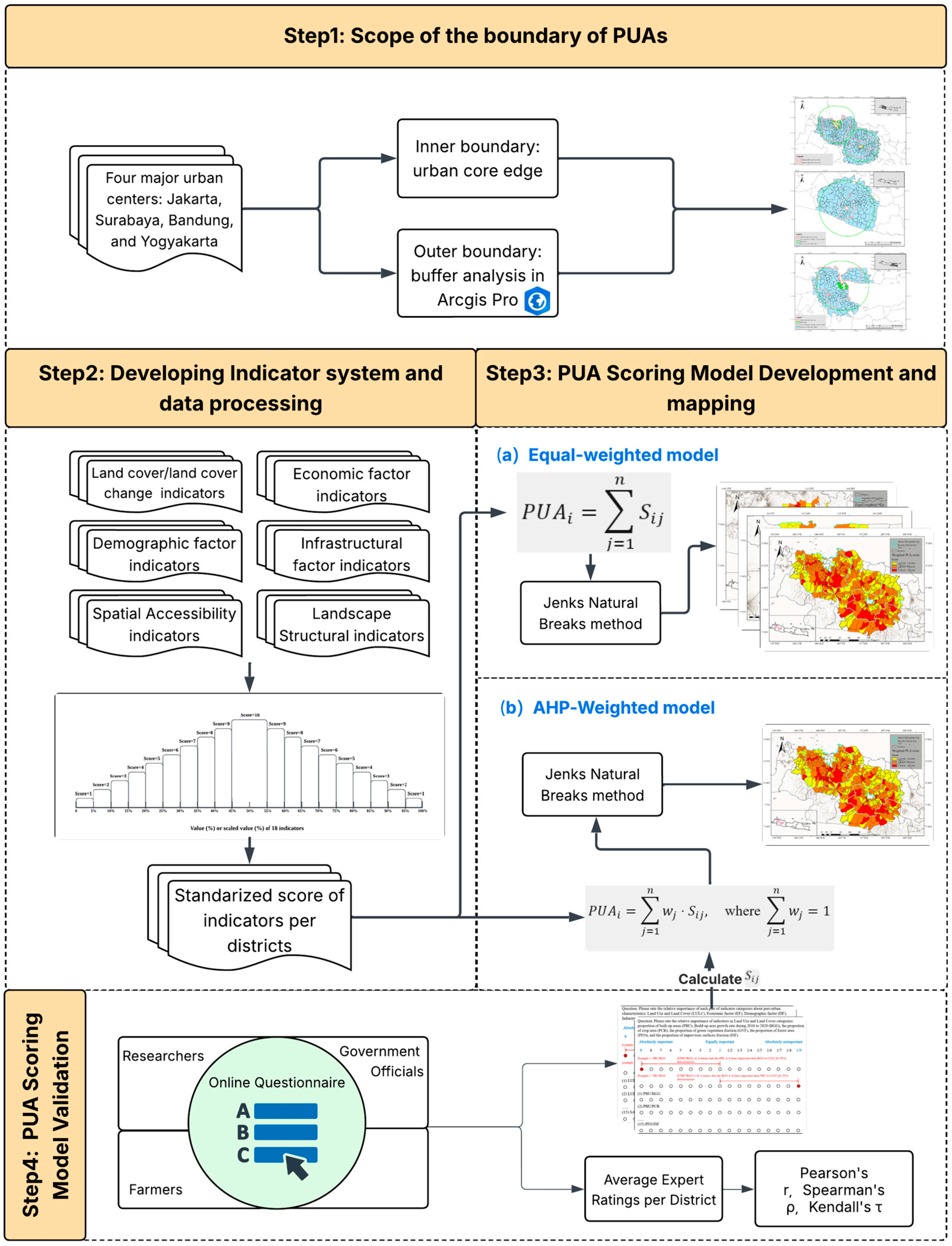
Figure 1. Flowchart with the main methodological processes carried out.
Remotesensing 18 01062 g001
Figure 2. The location of the study area is on Java Island, Indonesia, focusing on four major cities: Jakarta, Bandung, Yogyakarta, and Surabaya.
Remotesensing 18 01062 g002
Figure 3. PUA thresholds and scoring for 18 indicators.
Remotesensing 18 01062 g003
Figure 4. Example of a questionnaire item for pairwise comparison of primary-level indicator categories in PUA determination. Respondents rated the relative importance of indicator pairs (e.g., land use and land cover (LULC) vs. economic factors (EF)) using a 1–9 scale following the AHP framework.
Remotesensing 18 01062 g004
Figure 5. Example of a questionnaire item for pairwise comparison of secondary-level indicators within the Land Use and Land Cover (LULC) category. Respondents evaluated the relative importance of indicator pairs (e.g., proportion of built-up areas [PBU] vs. build-up area growth rate [BGG]) using a 1–9 scale under the AHP framework.
Remotesensing 18 01062 g005
Figure 6. The PUA boundaries of Jakarta and Bandung were identified by buffering analysis.
Remotesensing 18 01062 g006
Figure 7. The PUA boundaries of Yogyakarta were identified by buffering analysis.
Remotesensing 18 01062 g007
Figure 8. The PUA boundaries of Surabaya were identified by buffering analysis.
Remotesensing 18 01062 g008
Figure 9. Classification of PUAs around the Jakarta and Bandung Metropolitan Areas based on scores derived from the equal-weighted model. Districts are categorized into three levels: low (≤51), medium (52–64), and high (≥65).
Remotesensing 18 01062 g009
Figure 10. Classification of PUAs around the Jakarta and Bandung Metropolitan Areas based on scores derived from the AHP-weighted model. Districts are categorized into three levels: low (≤2.8624), medium (2.862401–3.7082), and high (≥3.7082).
Remotesensing 18 01062 g010
Figure 11. (a) Distribution of districts by PUA score levels in the Equal-weighted model for the Jakarta and Bandung Metropolitan Areas. Districts are classified into three categories: high (≥65), medium (52–64), and low (≤51). (b) Distribution of districts by PUA score levels in the AHP-weighted model for the Jakarta and Bandung Metropolitan Areas. Districts are classified into three categories: low (≤2.8624), medium (2.862401–3.7082), and high (≥3.7082).
Remotesensing 18 01062 g011
Figure 12. Classification of PUAs around the Yogyakarta Metropolitan Area based on scores derived from the equal-weighted model. Districts are categorized into three levels: low (≤52), medium (53–67), and high (≥68).
Remotesensing 18 01062 g012
Figure 13. Classification of PUAs around the Surabaya Metropolitan Area based on scores derived from the equal-weighted model. Districts are categorized into three levels: low (≤45), medium (46–60), and high (≥61).
Remotesensing 18 01062 g013
Table 1. Weight coefficients of PUAs’ primary-level indicator categories and PUAs’ secondary-level indicators 1.
Primary-Level IndicatorSecondary-Level IndicatorOverall Weight
LULC (0.2)PCR (0.22)0.04
GVF (0.19)0.04
PBU (0.18)0.04
PFA (0.13)0.03
ISF (0.11)0.02
BGG (0.17)0.03
EF (0.19)NEI (0.66)0.13
NLI (0.34)0.06
DF (0.16)PDB (0.51)0.08
PGG (0.49)0.08
IF (0.16)ART (0.35)0.06
CRD (0.25)0.04
LRD (0.2)0.03
NPF (0.2)0.03
SA (0.16)DTC (0.74)0.12
DTF (0.26)0.04
LS (0.13)BPD (0.64)0.08
PDN (0.36)0.05
1 LULC = Land Use and Land Cover; EF = Economic Factor; DF = Demographic Factor; IF = Infrastructure Factor; SA = Spatial Accessibility; LS = Landscape Structure; PCR = Proportion of Cropland; GVF = Proportion of Green Vegetation Fraction; PBU = Proportion of Build-up Area; PFA = Proportion of Forest Area; ISF = Proportion of Impervious Surface Fraction; BGG = Build-up Growth Rate during 2010 to 2020; NEI = Number of Economic Resources per area; NLI = Night Light Intensity in 2020; PDB = Population Density; PGG = Population Growth Rate from 2010 to 2020; ART = Arterial Road Density; CRD = Collector Road Density; LRD = Local Road Density; NPF = Number of Public Facilities per area; DTC = Distance to City Center; DTF = Distance to Forest; BPD = Built-up Area Patches Density in each district; PDN = Patch Density.
Table 2. Consistency between Mscore and Qscore for the equal-weight model and the AHP-weighted model.
Model TypeConsistency MetricValuep-Value
Equal weight modelPearson’s r0.5170.008
Spearman’s ρ0.5220.008
Kendall’s τ0.3870.008
Weighted modelPearson’s r0.3430.094
Spearman’s ρ0.3890.055
Kendall’s τ0.2840.047
Table 3. Cross-tabulation of district classifications between the equal-weighted and AHP-weighted models for districts within the 50 km buffer zones of Jakarta and Bandung (n = 416). Diagonal cells indicate classification agreement. Overall agreement = 65.1%; Cohen’s Kappa = 0.46.
AHP-Weighted Model
Equal-Weighted ModelHighMediumLowTotalAgreement (%)
High62431211753.0%
Medium161183617069.4%
Low3359112970.5%
Total81196139416
Table 4. Mean values of peri-urban indicators across four cities, cross-city SD, weight in AHP model, and weight–variability mismatch assessment. n is the number of districts within each city’s 50 km buffer zone.
Indicator 1Jakarta
(n = 216)
Bandung
(n = 200)
Yogyakarta
(n = 176)
Surabaya
(n = 175)
Cross-City
SD 2
Weight 3
PBU2.582.384.443.390.810.04
GVF6.747.798.566.700.780.04
LRD3.091.012.672.260.780.03
PDB3.411.931.591.860.710.08
NLI4.272.612.643.010.680.06
PFA2.043.432.341.710.650.03
PGG2.662.061.481.150.580.08
PCR3.755.025.214.890.570.04
BPD2.644.012.812.730.560.08
DTF2.433.592.262.340.540.04
ISF4.243.142.953.740.510.02
NFP1.841.072.142.060.420.03
ART2.732.152.231.880.310.06
BGG1.692.062.351.730.270.03
NEI1.731.711.211.350.230.13
CRD1.872.202.251.920.170.04
PDN3.463.363.223.630.150.05
DTC5.935.765.765.810.070.12
1 Indicator is 18 indicators used in equal and AHP models. PCR = Proportion of Cropland; GVF = Proportion of Green Vegetation Fraction; PBU = Proportion of Build-up Area; PFA = Proportion of Forest Area; ISF = Proportion of Impervious Surface Fraction; BGG = Build-up Growth Rate during 2010 to 2020; NEI = Number of Economic Resources per area; NLI = Night Light Intensity in 2020; PDB = Population Density; PGG = Population Growth Rate from 2010 to 2020; ART = Arterial Road Density; CRD = Collector Road Density; LRD = Local Road Density; NFP = Number of Public Facilities per area; DTC = Distance to City Center; DTF = Distance to Forest; BPD = Built-up Area Patches Density in each district; PDN = Patch Density. 2 Cross-city SD is the standard deviation of mean values of peri-urban indicators across the four cities, quantifying the degree of inter-city variability for each indicator. 3 Weight is the weight of the indicators in the AHP model.
Disclaimer/Publisher’s Note: The statements, opinions and data contained in all publications are solely those of the individual author(s) and contributor(s) and not of MDPI and/or the editor(s). MDPI and/or the editor(s) disclaim responsibility for any injury to people or property resulting from any ideas, methods, instructions or products referred to in the content.