Article

Estimating Grazing Land Acres Across the Contiguous United States Using Machine Learning Methods

1
Department of Statistics, Iowa State University, Ames, IA 50011, USA
2
USDA-ARS Jornada Experimental Range, Las Cruces, NM 88003, USA
3
USDA Natural Resources Conservation Service, Tucson, AZ 85719, USA
*
Author to whom correspondence should be addressed.
Retired.
Remote Sens. 2026, 18(7), 1050; https://doi.org/10.3390/rs18071050
Submission received: 27 January 2026 / Revised: 24 March 2026 / Accepted: 26 March 2026 / Published: 31 March 2026

Highlights

What are the main findings?
  • A new model estimates U.S. rangeland and pastureland acres with an average Area Under the Curve (AUC) greater than 0.90.
  • Satellite and survey data were integrated with machine learning to improve the precision of rangeland and pastureland acreage estimation.
What are the implications of the main findings?
  • Acreage estimates for user-defined geographic areas are obtained using flexible grid-based estimators.
  • Estimates of rangeland and pastureland extent support assessment of the condition and trends of grazing lands.

Abstract

Quantifying the extent of rangeland and pastureland (collectively termed grazing lands herein) in the US is a critical first step in many grazing lands assessments. This research presents a model-assisted framework to estimate grazing land acreage within arbitrary geographic boundaries by integrating high quality survey data with satellite-based raster geospatial data. Leveraging the image photo interpretation data from the USDA Natural Resources Conservation Service (NRCS) National Resources Inventory (NRI) survey as a reference dataset, we use machine learning to fuse NRI point level data with auxiliary data from the satellite-based Cropland Data Layer (CDL) to enhance the precision of acreage estimates of grazing lands. The methodology includes three steps: (1) modeling the relationship between NRI rangeland and pastureland indicators and CDL variables; (2) generating a high-resolution rangeland and pastureland probabilities map across the contiguous US; and (3) summarizing these probabilities to calculate the acreage of rangeland and pastureland for specific areas of interest. This approach provides researchers and land managers with a scalable tool to define grazing land extents within a self-selected study area, ensuring that subsequent resource characteristics or condition assessments are representative and spatially accurate.

1. Introduction

Rangelands and pasturelands are important agroecosystems that support livestock grazing, biodiversity, and provide key ecosystem services such as carbon storage and water regulation [1,2,3]. Rangeland and pastureland are two distinct grazing land cover categories, each characterized by the type of vegetation and management practices involved [4]. The USDA NRCS National Resources Inventory (NRI) defines rangeland as land where the climax vegetation is primarily native grasses, grass-like plants, forbs, or shrubs suitable for grazing/browsing, including areas naturally or artificially revegetated but managed like native rangelands, encompassing grasslands, savannas, shrublands, deserts, and tundra, and often characterized by physical limitations preventing cultivation. It supports natural plant communities, such as grasses and shrubs, that are often unsuitable for farming and are managed for forage production, even when planted with introduced species such as crested wheatgrass and managed using practices such as rotational grazing; the presence of livestock is not essential for classification [5]. In contrast, pastureland is managed primarily to produce introduced forage plants, often for livestock grazing. Pastureland cover may include single species or mixtures of grasses and legumes, and its management generally involves intensive cultural treatments such as fertilization, weed control, reseeding, and grazing management [5]. Unlike rangeland, pastureland is more actively managed for agricultural purposes, including livestock grazing and erosion control. Collectively, rangeland and pasturelands are referred to as grazing lands.
Understanding the extent of grazing lands and how they are changing in response to management and disturbance is critical for successful conservation planning. Monitoring these dynamics allows researchers and policymakers to identify trends in land use [6], assess ecosystem health [7], and develop strategies to promote sustainable land management [8,9]. For example, the USDA Natural Resources Conservation Service’s (NRCS) National Resources Inventory (NRI) survey provides comprehensive data on land cover and land use, including trends in pastureland and rangeland extent, condition, and transitions over time [10]. These data are invaluable for assessing the impact of agricultural practices, policy interventions, and environmental changes on grazing land resources across the United States.
Consistently and correctly identifying grazing lands in the US remains a challenge. While several widely used maps exist, challenges remain due to inconsistencies across definitions and classification systems. Ref. [11] highlight the fragmented and inconsistent methodologies used to estimate rangeland extent across the United States, particularly stemming from differing criteria applied by federal agencies such as NRI and the US Forest Service Forest Inventory and Analysis (FIA) programs. Although datasets like the Cropland Data Layer (CDL) and the National Land Cover Database (NLCD) provide land cover classifications that include rangeland- and pastureland-relevant categories, they have important limitations. Notably, neither CDL nor NLCD explicitly identifies “grazing lands” in the ecological sense recognized by NRCS or FIA. For more accurate and policy-relevant estimations, specialized data sources such as NRI or FIA-derived models are preferred because NRI provides field-validated land-use classifications that directly distinguish rangeland and pastureland. FIA, although useful for vegetation structure and ecological attributes, is designed for forest monitoring and contains limited sampling in non-forest landscapes. As a result, FIA cannot accurately characterize grazing lands on its own, leaving NRI as the most suitable dataset for reliable acreage estimation. In this study, we utilize the NRI because it offers two key advantages. First, it provides higher accuracy than CDL and NLCD, both of which rely solely on satellite imagery [12]; in contrast, the NRI uses low-altitude aerial photographs supplemented by local ground truthing and administrative records, resulting in a more reliable representation of ground conditions. Second, NRI supplies a transparent and internally uniform definition of rangeland and pastureland. This does not remove the cross-agency definitional variation noted by [11], but it ensures that our estimates rely on a single, consistently applied framework rather than mixing definitions across sources.
While NRI grazing land extent estimates are consistent, they are not comprehensive across the United States. This is because the NRI survey is designed to describe non-federal lands at the state level [13]. Therefore, attempts to quantify grazing lands for other land ownerships (i.e., federal) using the NRI data alone may be hampered by a low amount or lack of available training data in these land ownerships. Similarly, there may be inadequate samples to estimate the extent of grazing lands in other boundaries beyond states due to limited samples in an area of interest (e.g., EPA Ecoregion Level III for example). As a result, conservation planning and land management are limited because analyses cannot adequately and completely incorporate the extent of grazing land information at relevant scales of interest. These challenges motivate the need for a model-based framework that can combine NRI sample information with spatially explicit auxiliary data to support estimation of grazing land extent from local to national scales in the United States.
Recent land-cover mapping studies have increasingly relied on high-resolution remote sensing products for spatial classification. In addition to CDL, other products such as the National Land Cover Database (NLCD), ESA WorldCover, and Dynamic World are also relevant for grazing-land applications [14,15,16,17,18,19,20,21,22]. As summarized in Table 1, ESA WorldCover and Dynamic World provide global 10 m products, whereas CDL and NLCD are U.S.-focused land-cover products [15,17,19,22]. A key distinction lies in thematic specificity. ESA WorldCover and Dynamic World rely on broad grass-related classes and do not provide an explicit rangeland indicator [20,21]. Similarly, NLCD includes general land-cover categories such as grassland/herbaceous and pasture/hay but does not directly distinguish pastureland from rangeland in a manner consistent with the NRI definitions [18]. By comparison, CDL includes a Grass/Pasture category and provides greater agricultural specificity for the U.S. landscape, although it still does not directly separate pastureland from rangeland [14,15]. For this reason, CDL remains a practical auxiliary source for the current NRI-integrated framework because it is spatially explicit and agriculturally detailed, while NLCD, ESA WorldCover, and Dynamic World may provide useful complementary information in future work.
Beyond the choice of auxiliary data source, recent studies on land-cover mapping have increasingly relied on both traditional machine learning and deep learning methods for spatial classification using multi-source remote sensing data. On the machine learning side, widely used classifiers include Random Forest, support vector machines, and gradient-boosting methods, often combined with Sentinel or Landsat imagery and auxiliary variables to improve land-cover classification accuracy [23]. On the deep learning side, recent work has emphasized semantic-segmentation architectures such as U-Net, DeepLabV3+, and related CNN-based models for more detailed land-cover mapping from satellite imagery [24,25].
In parallel, the small area estimation literature has moved beyond classical direct estimation toward more spatially explicit and flexible model-based approaches. Recent work has incorporated spatial dependence and graph-based learning methods to improve estimation for fine-scale domains with sparse or imbalanced data [26,27]. These developments are relevant here because the present study also seeks to improve estimation for domains where direct sample support may be limited.
Against this background, our study combines NRI sample information with spatially referenced auxiliary land-cover data to support model-based acreage estimation for user-defined domains. Rather than focusing only on pixel-level classification accuracy, the proposed framework is designed to connect land-cover prediction with domain-level estimation, placing this work at the intersection of remote sensing classification, spatial prediction, and model-based small area estimation.
The goal of this project is to develop a statistical framework that integrates NRI data with satellite-based data to estimate grazing land acreage across specified geographies, and to apply this framework to quantify the extent of non-federal grazing lands in the United States. Although our analysis focuses on non-federal lands, the proposed approach is sufficiently flexible to be extended to other land ownership categories. By leveraging the NRCS NRI aerial survey data, small area estimation methods, and machine learning techniques, we aim to produce high-resolution probabilistic maps of rangelands and pasturelands. This work will provide a foundation for conservation planners, land managers, and scientists to assess grazing land conditions and trends and to support informed conservation planning.
The remainder of this paper is structured as follows. Section 2 provides a comprehensive overview of the National Resources Inventory (NRI) survey and the Cropland Data Layer (CDL) dataset. This section also describes the model setup and introduces the model-based imputation estimator employed in this study. Section 3 presents the results of the model comparison, including rangeland estimation and pastureland estimation at the Level III ecoregions. Section 4 provides a comprehensive discussion of the findings, highlighting their potential broader significance in advancing knowledge in the field. Section 5 outlines the implications of the research, emphasizing its significance for scientific advancements and practical applications in rangeland and pastureland management.

2. Materials and Methods

In this section, we develop a statistical framework to improve estimates of rangeland and pastureland acreage by integrating NRI sample points with spatially referenced CDL data [28] and to also allow users to define their geographic area(s) of interest, which is not possible under the existing acreage estimation process. The overall framework consists of three stages: data processing, modeling, and estimation of grazing land extent.
For data processing, we extracted a square tile of CDL pixels centered on the pixel containing each NRI sample point and quantified the proportion of each CDL land cover category within the tile. These proportions served as predictor variables, while the NRI classification for each sample point served as the response variable.
For modeling, we employed a supervised learning pipeline and trained several classification algorithms, including Random Forest, LightGBM, support vector machines (SVM), LASSO, and logistic regression, using 10-fold cross-validation. Model performance was assessed using both the area under the receiver operating characteristic curve (AUC) and cross-entropy loss. Models achieving high AUC and low cross-entropy were preferred, reflecting strong classification performance and accurate probability estimates. State-level NRI estimates were used as the primary benchmark for model evaluation. Because the NRI program reports official statistics at the state level, and county-level estimates are often less reliable due to smaller sample sizes and higher variability, state-level estimates provide the most robust basis for validation.
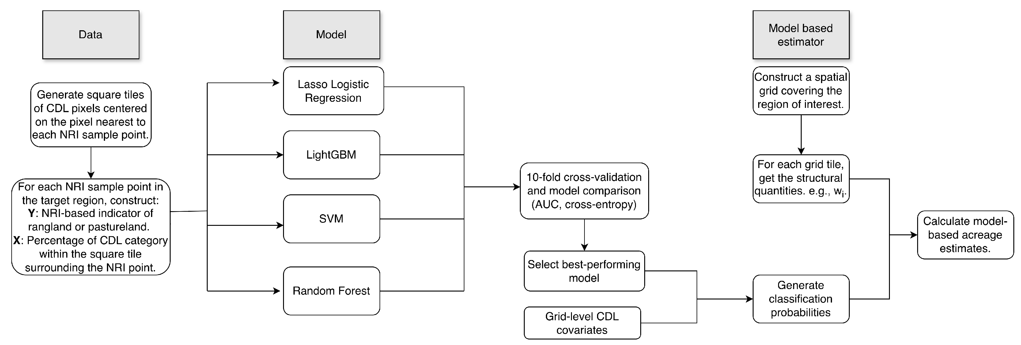
For estimation of grazing land extents, the selected model was deployed across a spatial prediction grid. CDL-derived covariates were generated for each grid cell to produce probabilistic estimates of rangeland and pastureland presence. These probabilities were then aggregated over the region of interest to derive model-based acreage estimates. This approach produces spatially explicit, model-based land cover estimates while remaining consistent with NRI definitions and state-level benchmarks. Figure 1 illustrates the three stages of the framework, each of which is discussed in detail in Section 2.1, Section 2.2 and Section 2.3.

2.1. Data Processing

2.1.1. NRI Photo Interpretation Data

In this study, we utilize the 2017 release of the Natural Resources Conservation Service’s (NRCS) National Resources Inventory (NRI) as the training dataset. The NRI is a longitudinal panel survey of land use and associated natural resource conditions, administered by the NRCS in collaboration with Iowa State University. It employs a stratified sample design and collects data primarily through the interpretation of aerial photography, supplemented by local ground truthing and administrative records. From 1982 to 1997, data were collected at five-year intervals for the full foundation sample of approximately 300,000 segments. Since 2000, the survey has been conducted annually using a rotating panel of approximately 70,000 segments per year [13]. In this study, we used the 2017 NRI dataset, which reflects the most recent update available at the time of analysis.
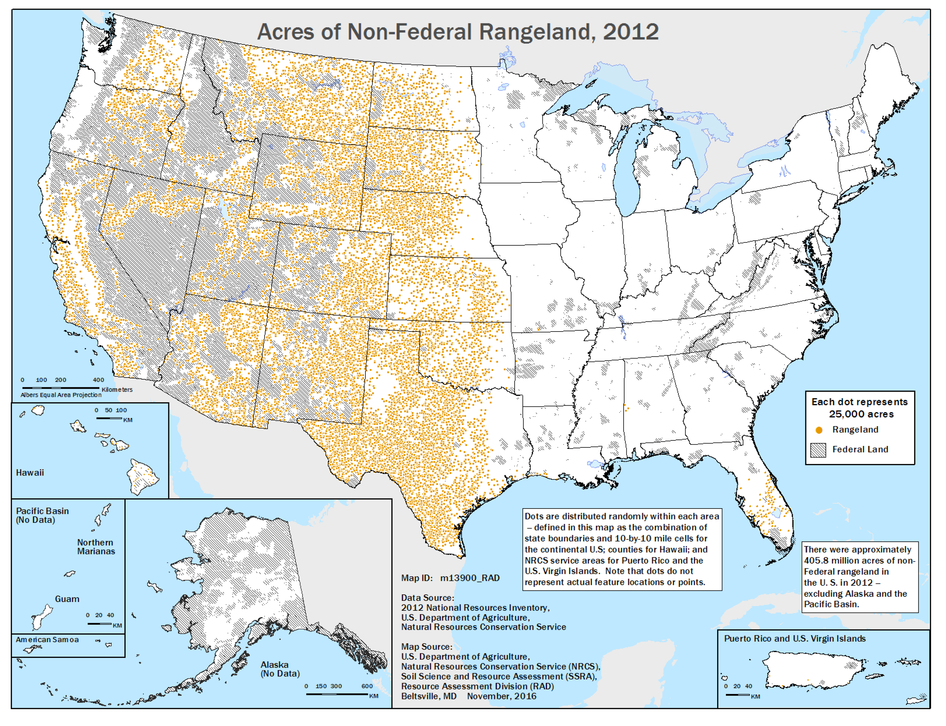
Figure 2 presents the spatial distribution of non-federal rangeland acreage in the contiguous United States in 2012, based on the USDA National Resources Inventory [29]. We use the publicly available 2012 rangeland map, as no corresponding public publication is available for 2017 that separately identifies rangeland points for non-federal lands. Nevertheless, we expect the spatial distribution of rangeland points in 2012 to be broadly similar to that in 2017, a conjecture that is supported by the consistency observed in our subsequent results. This dot-density map provides a quantitative visualization, where each dot represents approximately 25,000 acres of rangeland randomly distributed within predefined mapping units. It is crucial to note that these dots are cartographic representations and do not denote precise geographic locations. Consequently, they cannot be aggregated to compute rangeland acreage at Ecoregion Level III or any small geographical region, as the lack of spatial precision would introduce significant measurement error.
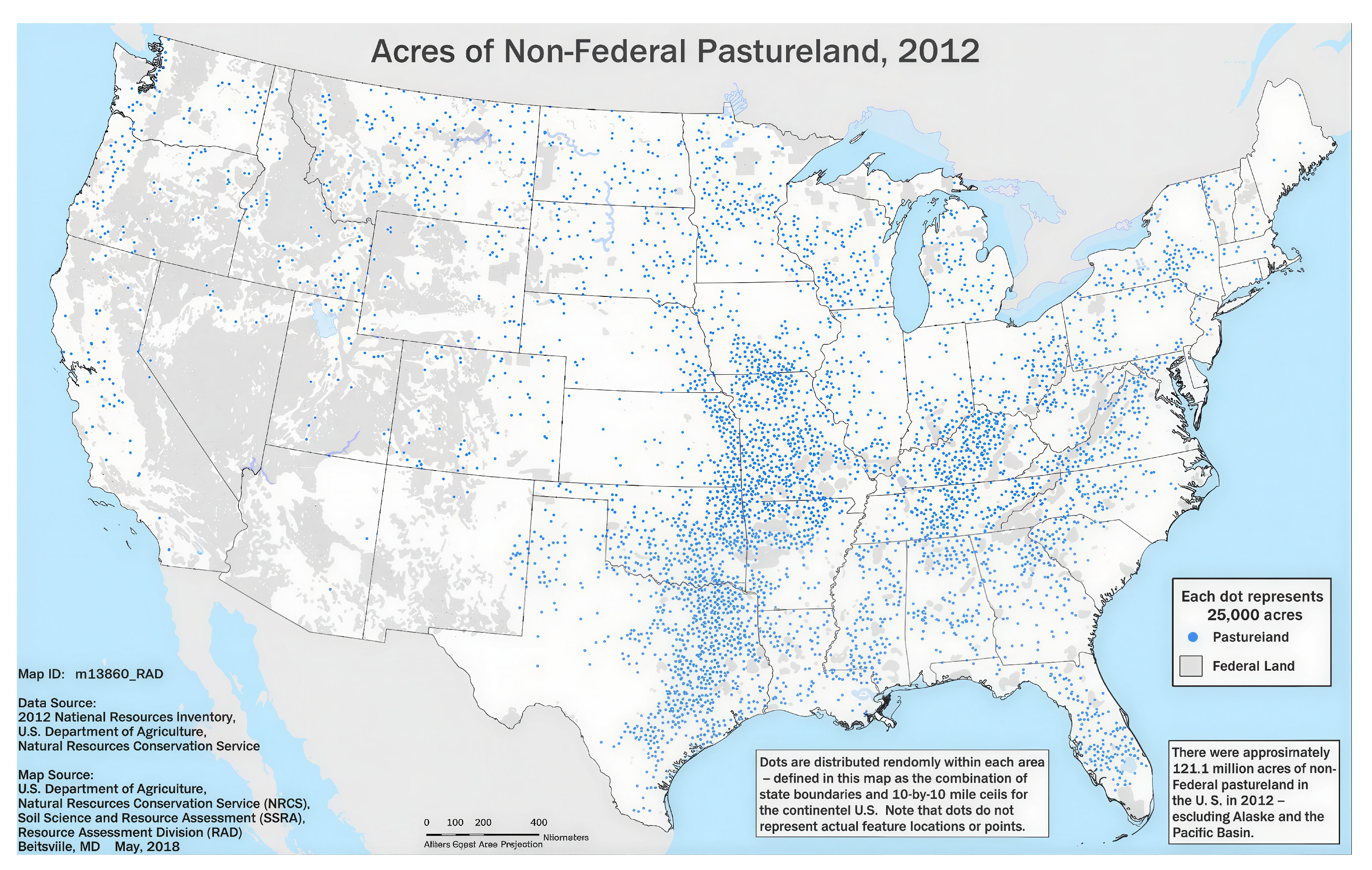
Figure 3 plots the spatial distribution of non-federal pastureland acreage based on the 2012 NRI data. In contrast to the western concentration of rangeland, non-federal pastureland exhibits a more dispersed pattern across the central and eastern United States [29]. The 2012 pastureland map is used because it represents the most recent publicly available source that explicitly delineates non-federal pastureland points; an analogous public map for 2017 is not available. Although the map predates the primary analysis year, the broad spatial patterns observed here are consistent with the pastureland distribution reflected in our later results, suggesting limited change in the overall geographic configuration.
This study uses rangeland and pastureland indicators (binary) from the 2017 NRI survey as the response variables Y. Table 2 reports the 2017 NRI sample sizes for each of the seventeen states included in the rangeland analysis, along with the corresponding number of points classified as rangeland. For the pastureland analysis, Table 3 summarizes the NRI sample sizes and the corresponding counts of pastureland points for all 48 contiguous U.S. states.

2.1.2. Cropland Data Layer Data

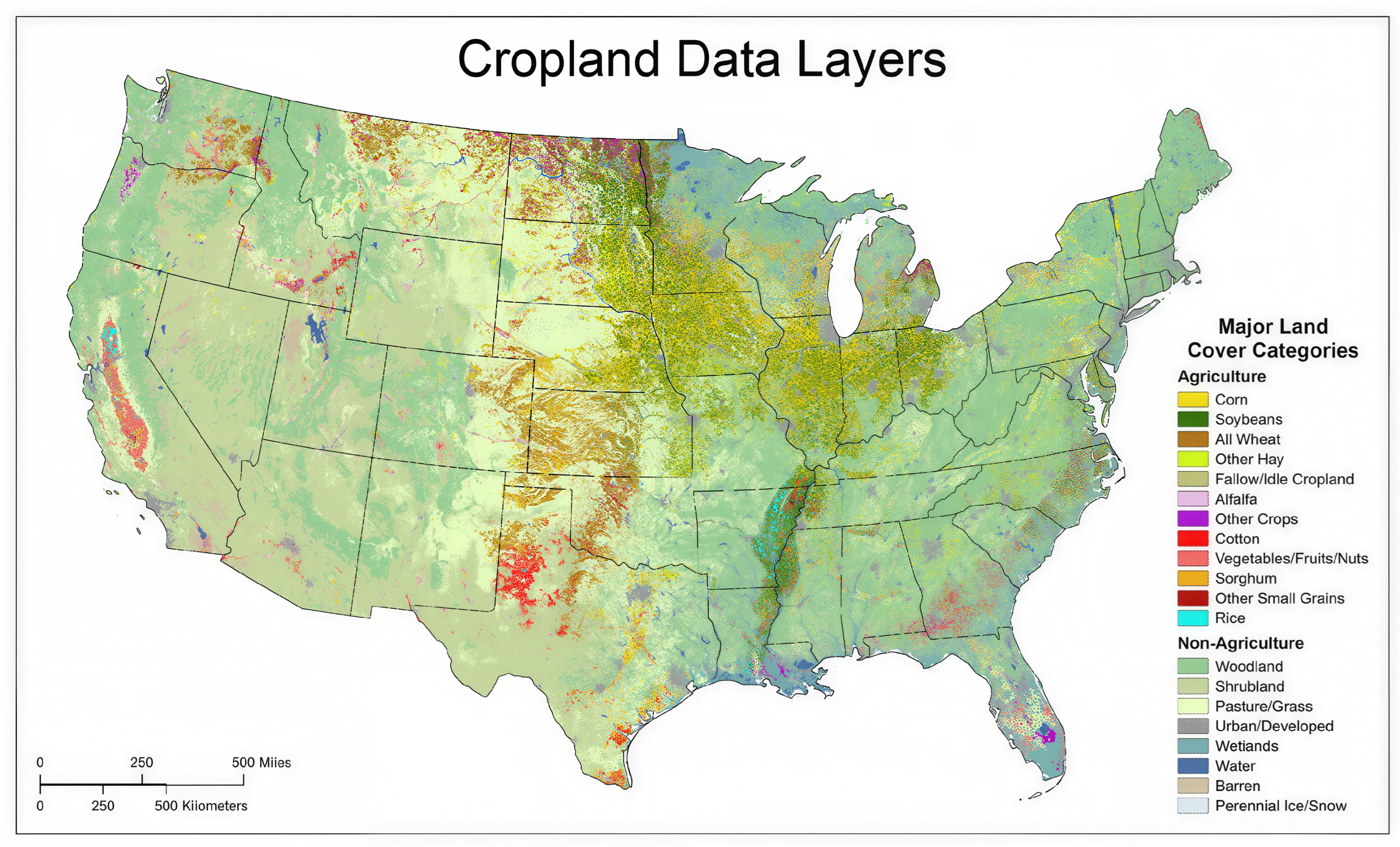
We used the Cropland Data Layer (CDL) to obtain predictor variables for our grazing land classification model. The CDL is a georeferenced raster product developed by the USDA’s National Agricultural Statistics Service (NASS) [12], providing annual land cover and crop-specific classifications for the contiguous United States. It is derived from remote sensing data, offering spatial resolutions of either 30 or 56 m, depending on the year and region [30]. Figure 4 presents the CDL, which provides a nationwide, raster-based classification of land cover and crop types across the contiguous United States. The CDL distinguishes major agricultural categories and non-agricultural land-cover classes, including pasture/grassland, shrubland, and woodland. In this study, the CDL serves as auxiliary information used to characterize local land-cover composition around NRI sample locations and to support model-based estimation of rangeland and pastureland extent. We utilized the 2017 CDL data, which provides 169 distinct land cover categories at a 30-m resolution, all of which were included as predictors in our model. These data were integrated with the 2017 NRI survey data.
Following the framework proposed by [28], we extracted CDL information using 7 × 7 pixel tiles centered on each NRI point, where each pixel represents a 30 × 30 m area. This tile size has been shown to yield optimal model performance. For each tile, we computed the proportion of pixels belonging to each CDL land-cover category, and these proportions were used as predictors in models relating CDL-derived variables (X) to rangeland or pastureland indicators (Y). Appendix A describes the spatial construction of these CDL-based predictors, the indexing scheme used to preserve spatial configuration, and the rationale for tile size selection.
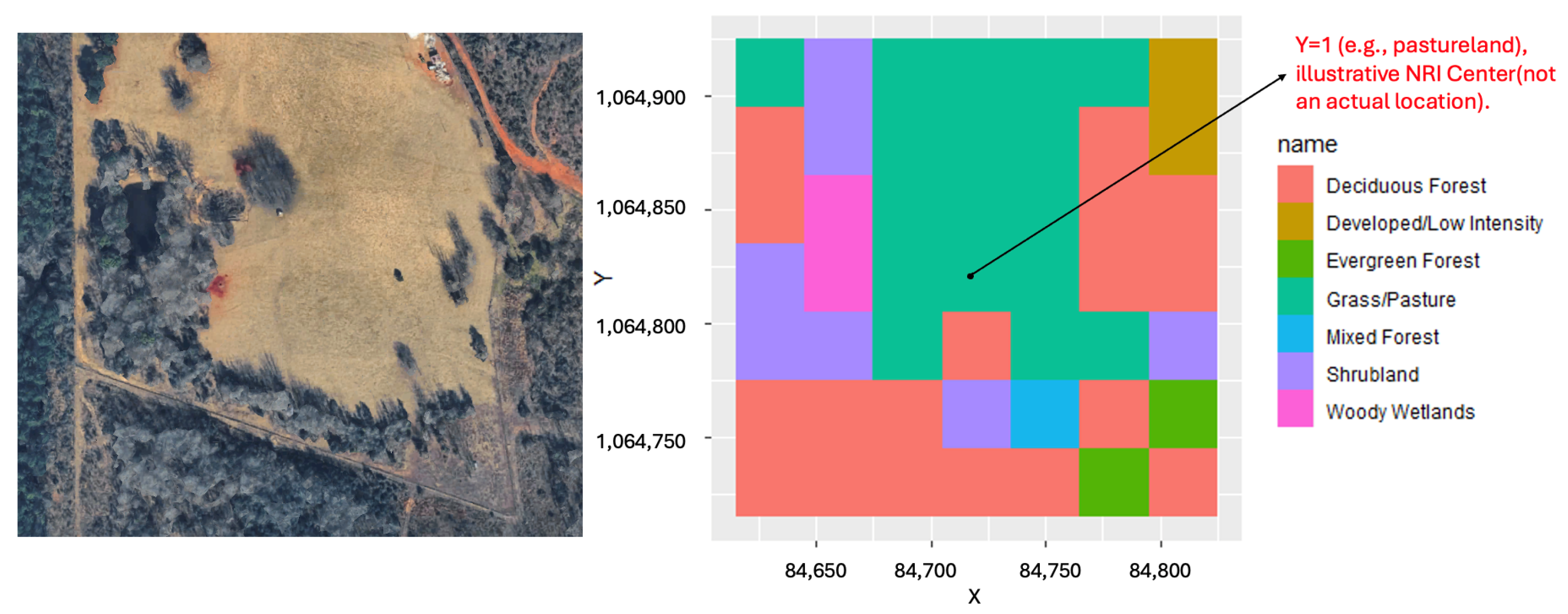
To provide a visual example of the data-generating process, Figure 5 illustrates how CDL information is extracted and organized for model input. Left panel shows a screenshot from Google Earth for a representative location, serving as a reference for the underlying land-surface features, while right panel depicts the corresponding 7 × 7 pixel grid of CDL land-cover categories used in the analysis. This example demonstrates how spatially explicit land-cover information from CDL is summarized at the tile level to construct predictor variables for estimating rangeland and pastureland extents.
The final dataset used for analysis consists of a binary indicator for rangeland or pastureland based on the NRI observation at the center of each tile, along with the proportions of CDL land-cover categories calculated within the 7 × 7 pixel tile, as illustrated in Figure 5.
The resulting sample-level dataset, consisting of CDL-derived predictor variables and NRI-based response labels, was then used as input for the classification models described in the next section.

2.2. Modeling the Relationship Between CDL Data and Rangeland and Pastureland Indicators

Based on the processed sample-level dataset described above, we next used a small area estimation (SAE) approach to predict the probability that a location is rangeland or pastureland using various machine learning models. In this subsection, we evaluate four machine learning methods to identify the optimal classifier for estimating rangeland and pastureland using the dataset described in Section 2.1. Section 2.2.1 provides a brief overview of the four methods, while Section 2.2.2 introduces the metrics used to assess model performance.

2.2.1. Machine Learning Methods

We evaluated the performance of four different machine learning approaches to identify the model with the best trade-off between bias and variance. Hyperparameters for all models were tuned via 10-fold cross-validation.
Logistic Regression with LASSO: Let i = 1 , , n index NRI sample locations. For each location, the response Y i { 0 , 1 } denotes the binary grazing-land indicator, where Y i = 1 indicates that the NRI point is classified as rangeland (or pastureland, depending on the analysis) and Y i = 0 otherwise.
Let X i = ( X i 1 , , X i p ) R p be the corresponding vector of CDL-derived predictors, where X i j is the jth predictor for location i. In our setting, X i j is constructed as the proportion of CDL pixels within the 7 × 7 tile centered at location i that are labeled as the jth CDL land-cover category, so that 0 X i j 1 . Although the CDL includes 169 possible land-cover categories, the effective predictor dimension p is region-specific and depends on the subset of categories observed within the region of interest. Only land-cover categories with nonzero representation in the surrounding CDL tiles are retained as predictors.
Given the binary response, logistic regression provides a natural baseline model. We model the conditional probability P ( Y i = 1 X i ) as
P ( Y i = 1 X i ; β ) = π ( X i ; β ) = exp β 0 + j = 1 p β j X i j 1 + exp β 0 + j = 1 p β j X i j ,
where β = ( β 0 , β 1 , , β p ) denotes the intercept and regression coefficients. To handle high-dimensional covaraiates in CDL data, we applied LASSO penalty to reduce the risk of overfitting [31]. LASSO imposes a penalty on regression coefficients, shrinking less informative predictors to zero, thereby performing feature selection and preventing overfitting.
LightGBM: To capture potential non-linear relationships, we include LightGBM, a gradient boosting framework based on decision trees [32], in our comparison. Light GBM grows tree leaf-wise. The split is performed on the leaf with the largest potential loss reduction, which typically results in faster training times and higher accuracy compared to traditional level-wise growth algorithms.
Support Vector Machines (SVM): SVM is another powerful supervised learning algorithm particularly well-suited for classification tasks [33]. It finds the optimal hyperplane that maximizes the margin between classes. SVM can handle non-linear classification through the use of kernel functions, which project the input space into higher dimensions. In this study, we tested various kernel functions (Radial Basis Function, polynomial, and sigmoid), and selected the best-performing kernel through cross-validation.
Random Forest: This ensemble method constructs a multitude of decision trees during training and outputs the mode of the classes [34]. By averaging predictions from trees trained on random subsets of data and features (bagging), Random Forest effectively reduce variance while avoid overfitting, making it a robust and reliable choice for complex datasets.

2.2.2. Model Comparison Methodology

Model performance was assessed using two complementary metrics: Area Under the Curve (AUC) and Cross-Entropy Loss (CE). The AUC measures a model’s ability to distinguish between binary classes—in this case, grazing land versus non-grazing land—across all possible decision thresholds. It summarizes the trade-off between the true positive rate and the false positive rate into a single scalar value and is independent of any particular classification threshold. An AUC of 0.5 indicates performance no better than random guessing, while an AUC of 1.0 reflects perfect classification. This threshold-independent property makes AUC particularly useful for comparing model performance in imbalanced classification settings.
AUC does not assess the quality of predicted class probabilities which are directly used in the acreage estimation. Therefore, we additionally used cross-entropy loss, which evaluates how closely the predicted probabilities align with the observed binary outcomes. We illustrate this criterion using Logistic Regression with Lasso. For the binary response Y i { 0 , 1 } , let p ^ i denote the fitted probability of observing Y i = 1 given covariates X i . Specifically, p ^ i is obtained by evaluating the logistic model in (1) at the estimated coefficient vector β ^ , that is,
p ^ i = π ( X i ; β ^ ) = exp β ^ 0 + j = 1 p β ^ j X i j 1 + exp β ^ 0 + j = 1 p β ^ j X i j .
Given p ^ i defined in (2), the cross-entropy loss is defined as
L CE = 1 N i = 1 N Y i log ( p ^ i ) + ( 1 Y i ) log ( 1 p ^ i ) .
Other classification methods considered in this study follow an analogous procedure, differing primarily in how β ^ or the corresponding fitted probabilities p ^ i are obtained; for brevity, their objective functions are not reproduced here.
Cross-entropy penalizes overconfident and poorly calibrated predictions and is particularly relevant in settings where predicted probabilities are subsequently used in model-based estimation. Together, AUC and cross-entropy provide a complementary assessment of both classification accuracy and probabilistic calibration.

2.3. Estimating Grazing Land Extents

This section addresses one of the study’s dual objectives by presenting a flexible framework for estimating rangeland and pastureland extents. The preceding section introduces a modeling approach that uses machine learning models to produce statistically consistent estimates of probability that a given location is rangeland (patureland) or not using the corresponding CDL information at that location. In this section, we extend that framework to user-defined geographic domains, allowing grazing land extent estimates to be aggregated over ecologically or administratively meaningful regions. Together, these features support more accurate interpretation of grazing land patterns in the context of conservation needs and spatial trends. We introduce the model-based estimator in Section 2.3.1. As a benchmark, Section 2.3.2 presents a design-based estimator that relies solely on survey data without incoorporating CDL information. Section 2.3.3 then describes the procedure used to calculate standard errors.

2.3.1. Model-Based Estimation

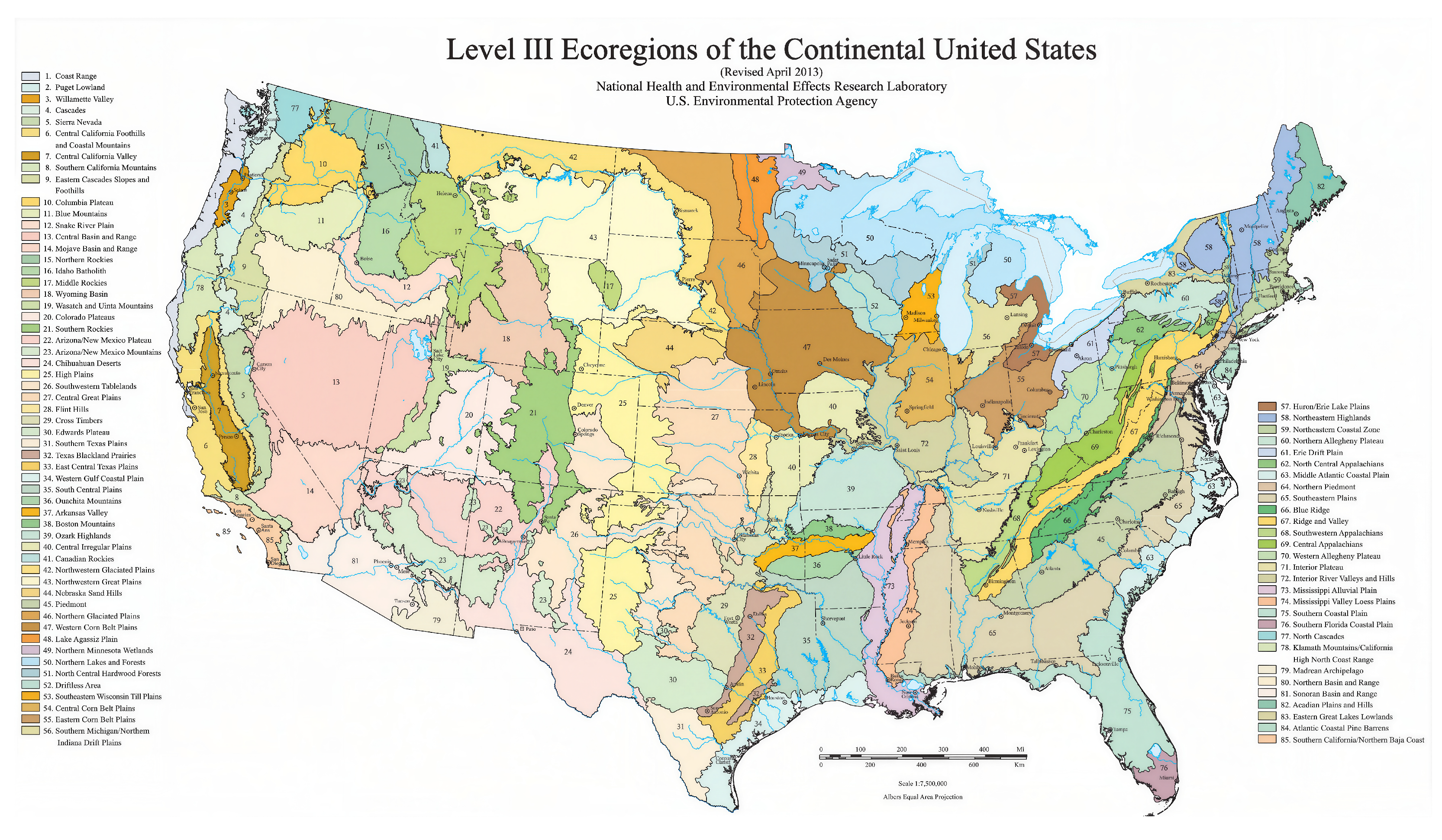
After developing the machine learning models, we apply the selected models to estimate the acreage of rangeland and pastureland within specified regions of interest. In this study, we transition the geographical units from U.S. states to an alternative regional delineation: Ecoregion Level III [35]. Ecoregions represent areas where ecosystems, including the type, quality, and quantity of environmental resources, share general similarities [36]. These regions serve as a crucial spatial framework for the research, assessment, and monitoring of ecosystems and their components. Ecoregions are essential for structuring and implementing ecosystem management strategies across various nongovernmental organizations that manage diverse resources within the same geographic areas. By transitioning to Ecoregion Level III, the study adopts a more ecologically relevant approach, better aligning with the natural distribution of resources and enhancing the effectiveness of management and conservation strategies. Moreover, the proposed modeling framework is flexible and can be readily extended to alternative geographic delineations, such as Land Resource Regions (LRRs) and Major Land Resource Areas (MLRAs) used by the USDA NRCS for soil surveying, land-use planning, and related applications. Figure 6 shows the spatial boundaries of the Level III ecoregions used in this study [37].
We apply the machine learning models separately within each ecoregion to estimate the probability that each location is rangeland (pastureland) or not. By repeating this process across all ecoregions, we generate a continuous probability map covering the entire United States (see Figure 14 in Section 3.2).
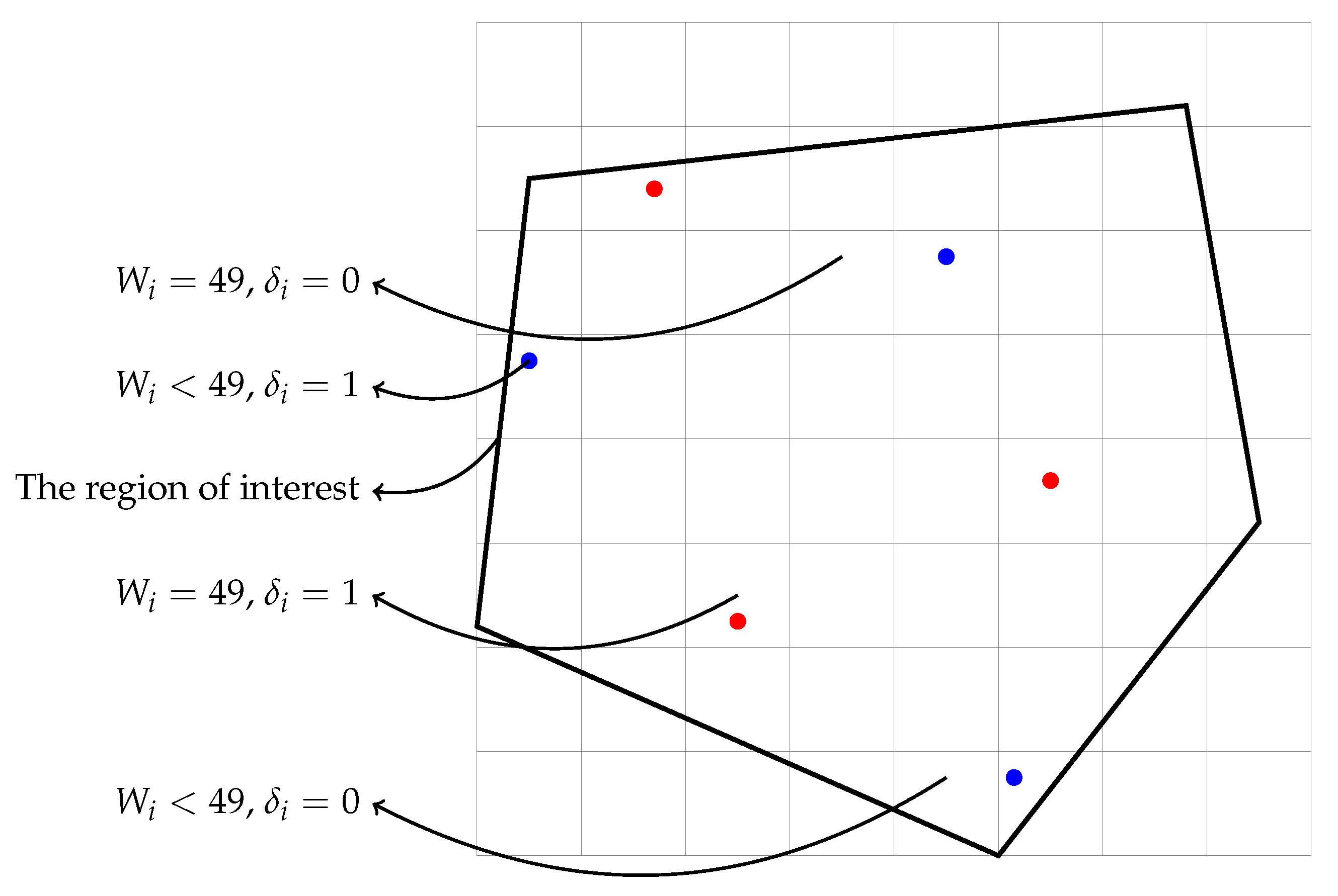
To estimate the rangeland (or pastureland) acres in a given geographical domain after obtaining the continuous probability map, we construct a grid of tiles that covers the region of interest, where each tile is a square consisting of 7 × 7 pixels [28]. Let N denote the total number of tiles that intersect with the region (e.g., an EPA Ecoregion, a Hydrologic Unit Area, etc.). For each tile, let W i represent the number of pixels within the ith tile that overlap with the region, with 0 < W i 49 for all i, W i = 49 indicates that the tile fully overlaps with the region, and W i < 49 indicates partial overlap. Additionally, we define δ i as an indicator variable that equals 1 if the grid cell contains at least one NRI sample point, and 0 otherwise. Figure 7 provides an illustration of the tiles and the corresponding overlap with the region of interest.
Since each pixel in CDL corresponds to 0.2223946 acres, we use m = 0.2223946 as the conversion factor to translate pixel counts into acres. It is important to note that NRI data on rangeland and pastureland are limited to non-federal lands and therefore exclude federally managed rangelands from the current analysis. However, the proposed approach is designed to be applicable to land areas irrespective of ownership. When the target geographic domain is restricted to either federal or non-federal lands, the final acreage estimates can be adjusted by excluding ineligible pixels using land ownership indicators during the final estimation stage. For this purpose, let η i denote the federal ownership indicator, where η i = 1 if the ith square tile is federally owned and η i = 0 otherwise. We define the true acreage of non-federal rangeland or pastureland within a given region as
T = i = 1 N m W i ( 1 η i ) Y i ,
where Y i is binary indicator for being rangeland or pastureland. The model-based estimator of T, denoted by T ^ m , is defined as
T ^ m = i = 1 N m W i ( 1 η i ) δ i Y i + ( 1 δ i ) E ^ [ Y i X i ] .
For a binary response, the conditional expectation E ^ [ Y i X i ] equals the estimated probability that Y i = 1 given covariates X i . Denote this estimated probability by p ^ i , as defined in Equation (2). Accordingly, the model-based estimator can be written as
T ^ m = i = 1 N m W i ( 1 η i ) δ i Y i + ( 1 δ i ) p ^ i ,
where p ^ i is obtained using the modeling approach described in the Section 2.2.1.

2.3.2. Design-Based Estimation

To validate the model-based estimation of rangeland and pastureland, we compare our estimates with those obtained from county- and state-level design-based estimates constructed using NRI data only. Let
T ^ s = i W ˜ i , s Y i , s
denote the NRI design-based estimator [38] of the total acreage of non-federal rangeland or pastureland in state s, where
Y i , s = 1 , if the i th NRI sample point in state s is classified as rangeland or pastureland , 0 , otherwise ,
and W ˜ i , s denotes the survey weight associated with the ith NRI sample point in state s, reflecting the area of non-federal land represented by that point. The NRI survey weights are constructed to represent non-federal land at the state level, ensuring that all weighted estimates correspond exclusively to non-federal lands within each state.
It is important to note that NRI samples were drawn to achieve target precision for rangeland and pastureland estimates at the state level. Consequently, when analyses are conducted at finer geographic scales, such as EPA Level III ecoregions, the number of available sample points may be limited.
To evaluate model performance, South Dakota and Arkansas were selected for analysis based on the availability of adequate NRI sample sizes to support model validation. South Dakota contains a substantial number of rangeland observations, while Arkansas provides sufficient pastureland samples, enabling reliable evaluation across both land-cover types.

2.3.3. Estimating Variance

We adopt the jackknife method to estimate the variance of T ^ m . The jackknife is particularly well-suited for settings with sparse data, as it does not rely on strong distributional assumptions.
Following NRI convention, we partition all CDL tiles within the area of interest into 29 systematic groups, a practice rooted in early NRI implementation and now widely adopted [38]. For each group k = 1 , , 29 , we recompute the model-based estimator T ^ k by excluding observations in the kth group from the data set. These replicate estimates are then used to construct the jackknife variance estimator. See [39] for a detailed discussion of jackknife replication methods and the computation of variance and standard errors based on replicated estimates.
Several EPA Level III ecoregions contain an insufficient number of NRI sample points classified as rangeland or pastureland, making it difficult to reliably fit the models within these regions. To address this limitation, we merge the affected ecoregions with adjacent regions so that the resulting model-based state-level estimates (obtained by aggregating over state boundaries) are as consistent as possible with the NRI-reported state-level estimates produced by the design-based approach. Appendix B describes the ecoregion combination procedure in detail.

3. Results

This section presents the empirical results of our modeling framework in two stages. In Section 3.1, we first conduct a systematic comparison of machine learning classifiers across various square tile sizes to evaluate predictive performance and identify the most reliable model–resolution combination for estimating rangeland and pastureland. This analysis assesses model accuracy using both threshold-independent and probabilistic performance metrics, providing the basis for model selection. Building on these results, we then extend the analysis to the Level III Ecoregion scale in Section 3.2, where the selected modeling approach is used to generate spatially explicit estimates of total rangeland and pastureland area. Together, these subsections establish the empirical justification for model choice and demonstrate its application to large-scale land-cover estimation.

3.1. Comparative Evaluation of Classifiers and Tile Resolutions

To evaluate the influence of tile sizes on model performance, we compare four spatial dimensions— 1 × 1 , 3 × 3 , 5 × 5 , and 7 × 7 —using the rangeland dataset from South Dakota and the pastureland dataset from Arkansas. The optimal tile size is determined based on the configuration that yields the highest area under the receiver operating characteristic curve (AUC). We also implemented a 10-fold cross-validation procedure to assess the predictive performance of four modeling approaches: LASSOmin, Light Gradient Boosting Machine (LightGBM), Support Vector Machine (SVM), and Random Forest. For each outer training set, model tuning was performed using only the training data to avoid information leakage from the held-out fold.
For LASSO, LASSOmin denotes the value of the penalty parameter that minimized the cross-validated loss. For LightGBM, hyperparameter tuning was conducted over the number of leaves, learning rate, number of boosting iterations, class-weight adjustment, and the minimum number of observations in a child node. For SVM, the tuning grid included the penalty parameter, kernel type, and kernel coefficient option. For Random Forest, the tuning grid included the number of trees, maximum tree depth, the minimum number of samples required to split an internal node, and the minimum number of samples required at a leaf node. For each tuned model, the optimal hyperparameter combination was selected using only the training data, with cross-validated AUC as the tuning criterion.
Table 4 summarizes the mean values of AUC in 16 different scenarios, comparing the performance of various models in different square tile sizes and modeling approaches. The AUC serves as a key metric for evaluating prediction accuracy, with higher values indicating better model performance.
For the rangeland dataset, the Random Forest model achieved an AUC exceeding 0.95, demonstrating excellent predictive accuracy. In particular, the combination of Random Forest with the 7 × 7 tile configuration provided the most robust framework for estimating the acreage of rangelands. In the case of the pastureland dataset, the results exhibited a consistent pattern: larger square tiles corresponded to higher AUC values, suggesting that increased spatial context enhances predictive capability. This observation is consistent with the findings of the rangeland analysis. Consequently, to estimate pastureland acreage, data derived from the largest tile size were utilized. Among all models assessed, Random Forest consistently achieved AUC values greater than 0.94, underscoring its strong classification performance and validating its selection as the preferred modeling approach for this analysis.
While the AUC results in Table 4 demonstrate strong predictive performance across different models and tile sizes, the evaluation is based on randomly partitioned cross-validation folds. Because land cover types often exhibit strong spatial continuity, nearby observations may be spatially correlated. When training and test samples are randomly split without accounting for spatial structure, evaluation metrics may be overly optimistic due to information leakage between neighboring locations.
To address this concern, we conducted an additional spatial cross-validation analysis when evaluating model performance. Specifically, we adopted a leave-county-out validation scheme in which approximately 10 % of counties were held out as the test set in each fold, while the remaining counties were used for model training. Because observations within the same county tend to be spatially clustered, this approach helps reduce the influence of spatial autocorrelation between training and testing samples and provides a more realistic assessment of predictive performance.
Table 5 reports the AUC values obtained under this spatial validation scheme. The results remain consistent with the main findings of this study: larger spatial tiles generally improve predictive performance, and the Random Forest model with a 7 × 7 tile achieves the highest AUC for both rangeland and pastureland classification. These results suggest that the proposed framework remains robust even under spatially structured validation.
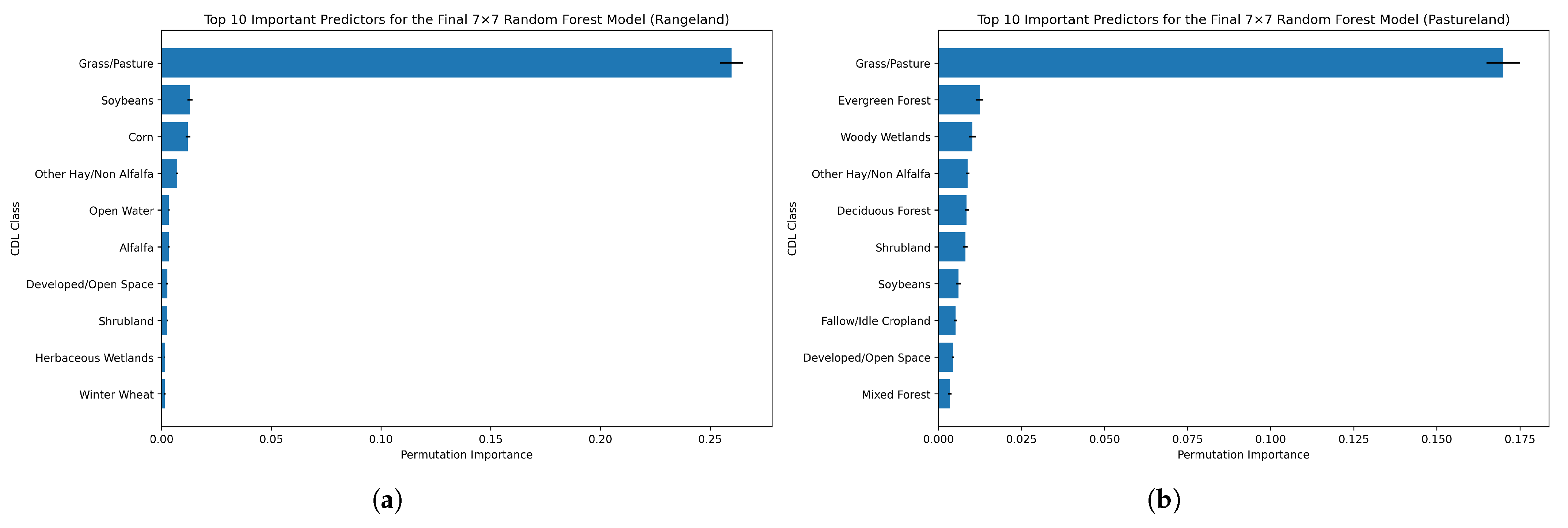
Based on the AUC evaluation results presented above, the 7 × 7 Random Forest model was selected as the best-performing classifier for both the rangeland and pastureland analyses. To further interpret the fitted models, we computed feature importance for the final rangeland model (South Dakota) and the final pastureland model (Arkansas). Feature importance was assessed using permutation importance, which measures the decrease in predictive performance after randomly permuting the values of a given predictor while leaving the remaining predictors unchanged. Predictors that cause a larger reduction in model performance when permuted are considered more influential in the fitted model.
Figure 8 summarizes the top 10 most important CDL-derived predictors for the selected 7 × 7 Random Forest models. In both panels, the CDL Grass/Pasture class is the dominant predictor, indicating that local grass-related land-cover composition plays the strongest role in distinguishing grazing land. At the same time, the remaining important predictors differ between the two models, suggesting that the surrounding land-cover context associated with rangeland classification is not identical to that associated with pastureland classification. For example, the rangeland model assigns relatively greater importance to cropland-related classes such as Soybeans and Corn, whereas the pastureland model gives relatively greater weight to forest- and wetland-related classes such as Evergreen Forest and Woody Wetlands. Nevertheless, the CDL Grass/Pasture class is not identical to the NRI pastureland definition used as the response variable in this study, so its strong importance does not imply that pastureland can be classified with uniformly high accuracy.
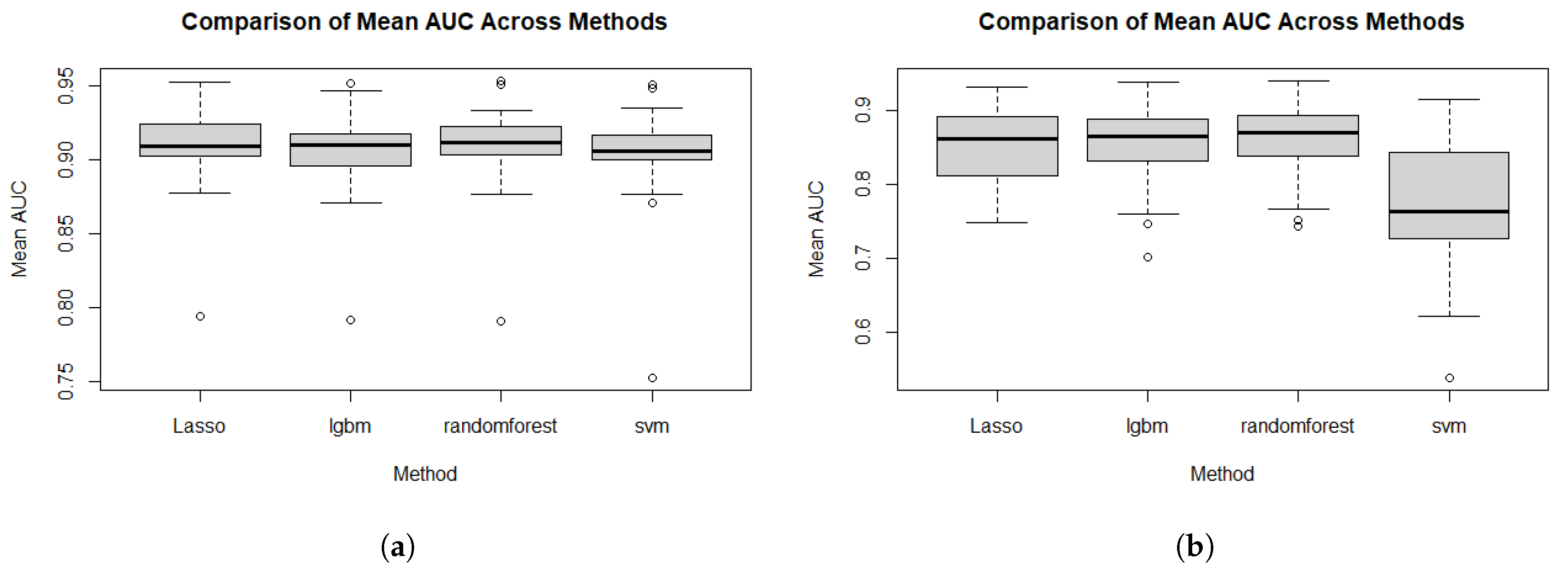
Using state boundaries as the domain of analysis, we evaluate model performance across 17 U.S. states for rangeland (Figure 9a) and 48 U.S. states for pastureland (Figure 9b). Model accuracy is assessed using mean AUC values computed for each state, with a 10-fold cross-validation procedure employed to ensure robust and reliable evaluation.
For the rangeland dataset, all models demonstrate relatively high AUC values, with Random Forest and LASSO exhibiting slightly higher median AUCs, reflecting strong classification capabilities across the analyzed states. The observed consistency and distribution of AUC values indicate that, although all models perform well, Random Forest stands out as particularly robust in predictive accuracy. In the case of pastureland, the Random Forest, LightGBM, and LASSO models display relatively consistent performance, characterized by higher median AUC values. In contrast, the SVM model shows greater variability and a lower median AUC, suggesting reduced reliability. These findings indicate that Random Forest, LightGBM, and LASSO offer more stable and accurate predictions for pastureland estimation across the 48 states, whereas SVM exhibits a broader performance range and lower overall effectiveness.
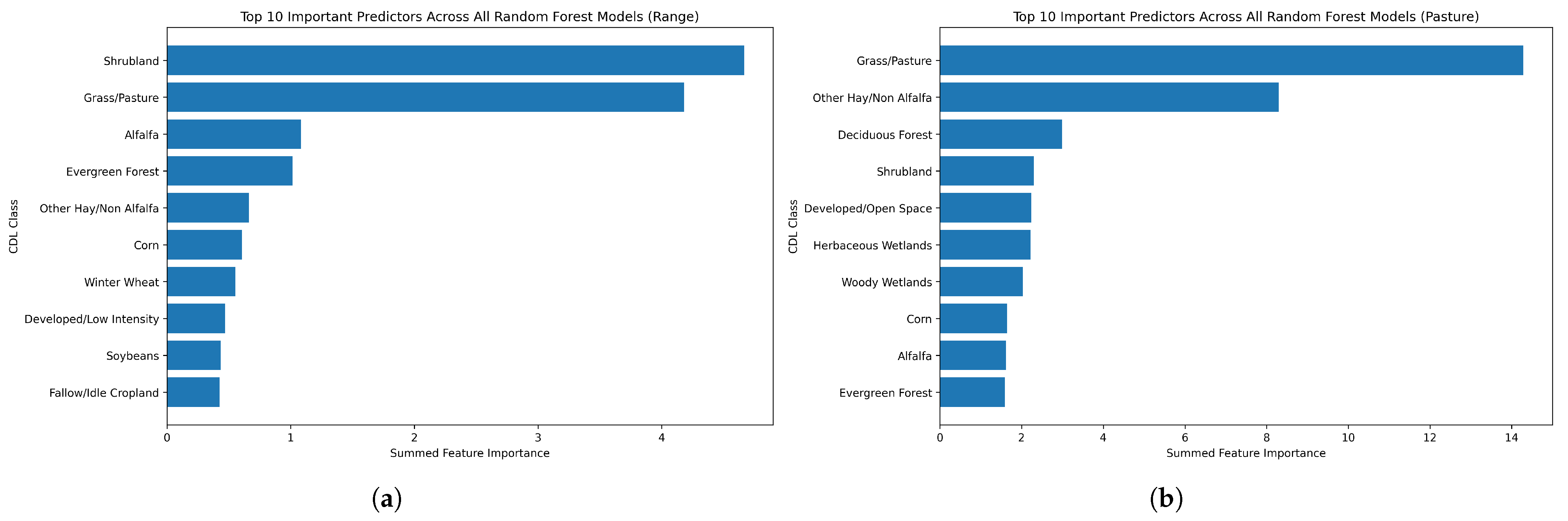
To further examine how important CDL-derived predictors vary across regions, we aggregated the feature importance values from the state-specific Random Forest models and summarized the top 10 predictors for rangeland and pastureland in Figure 10. Although this aggregation is intended as a descriptive summary rather than a formal inferential comparison, it provides a useful overview of the predictors that repeatedly contribute to classification across states. For pastureland, the CDL Grass/Pasture class is the dominant predictor by a substantial margin, followed by Other Hay/Non Alfalfa, suggesting that pastureland classification is most strongly associated with grass- and forage-related land-cover composition. For rangeland, Shrubland and Grass/Pasture emerge as the two most influential predictors, with additional contributions from classes such as Alfalfa, Evergreen Forest, and other cropland-related categories. These patterns indicate that, while the CDL Grass/Pasture class is important for both pastureland and rangeland, the broader land-cover context differs between the two, with pastureland showing stronger associations with forage and wetland/forest-adjacent classes and rangeland showing stronger associations with shrub-dominated and mixed surrounding landscapes. Overall, these results support the view that regional variation in land-cover composition contributes to differences in classification patterns across grazing-land types.
While AUC is widely used to assess classification performance, it evaluates only the relative ranking of predicted probabilities and is insensitive to probability calibration. Because our acreage estimator directly aggregates predicted probabilities, accurate probability estimation is critical. We therefore complement AUC with cross-entropy loss, which explicitly penalizes deviations between predicted probabilities and observed outcomes. Table 6 reports the mean cross-entropy values for rangeland and pastureland classification across four square tile sizes and four modeling approaches. Cross-entropy directly evaluates the quality of predicted probabilities, with lower values indicating better calibrated and more accurate probabilistic predictions.
For the rangeland dataset, all models exhibit decreasing cross-entropy as tile size increases, indicating that incorporating broader spatial context improves probabilistic performance. Among the methods considered, the Random Forest model consistently achieves the lowest cross-entropy across all tile sizes, followed closely by LASSO, while LightGBM and SVM exhibit comparatively higher loss values. A similar pattern is observed for the pastureland dataset, where larger tile sizes are associated with lower cross-entropy values across all models. Random Forest again demonstrates superior performance, yielding the lowest cross-entropy for each tile configuration. LASSO performs competitively, whereas SVM and LightGBM show higher loss, particularly for smaller tile sizes. Overall, these results suggest that Random Forest provides the most reliable probability estimates for both rangeland and pastureland classification, especially when larger spatial neighborhoods are used.
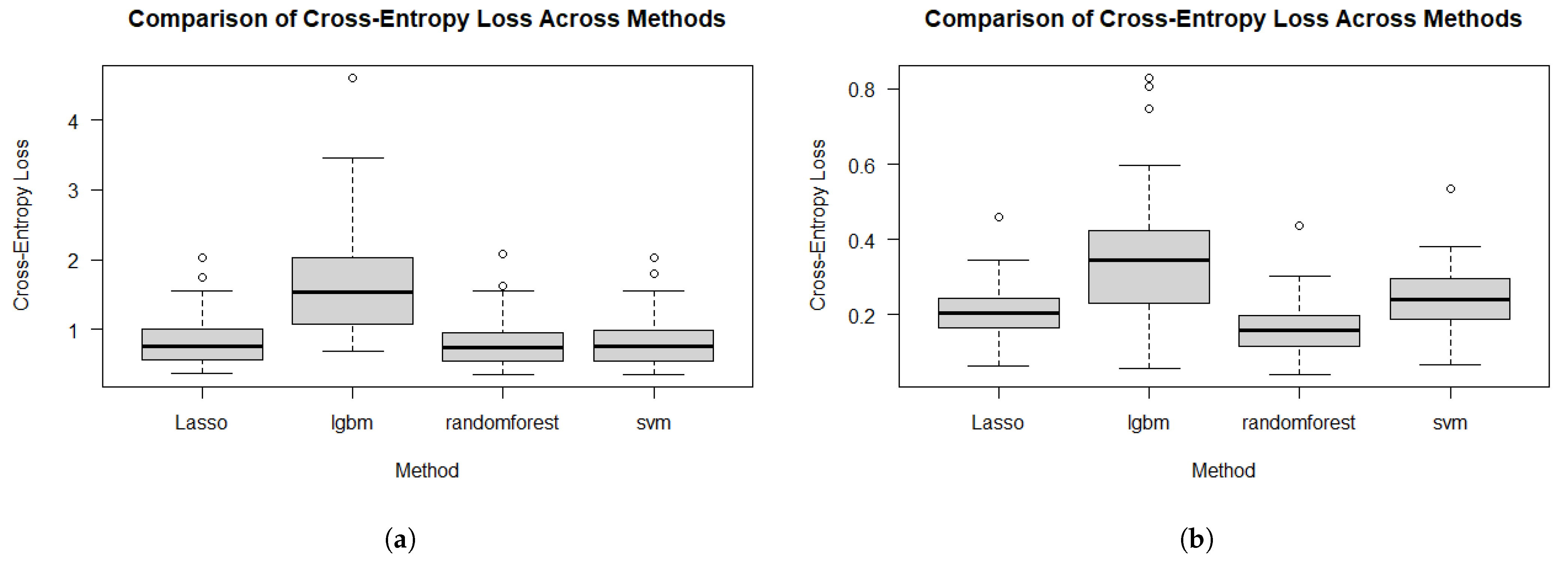
Figure 11 presents boxplots of cross-entropy values across states for four classification models. Lower cross-entropy values indicate better probabilistic calibration and predictive accuracy. In panel (a), corresponding to rangeland classification, the Random Forest model exhibits the lowest median cross-entropy and the narrowest interquartile range among the four methods, indicating both strong predictive performance and relatively stable behavior across states. LASSO and SVM yield moderately higher median losses with comparable dispersion, while LightGBM displays substantially higher median loss and greater variability, suggesting less consistent probability calibration in this setting. Panel (b) shows a similar pattern for pastureland classification across 48 states. Random Forest again achieves the lowest median cross-entropy, with limited dispersion, highlighting its robustness and reliability across a larger and more heterogeneous spatial domain. LASSO and SVM demonstrate intermediate performance, with slightly higher median losses and moderate variability. In contrast, LightGBM exhibits the highest median cross-entropy and the widest spread, indicating greater sensitivity to state-level heterogeneity and reduced stability in probabilistic predictions.
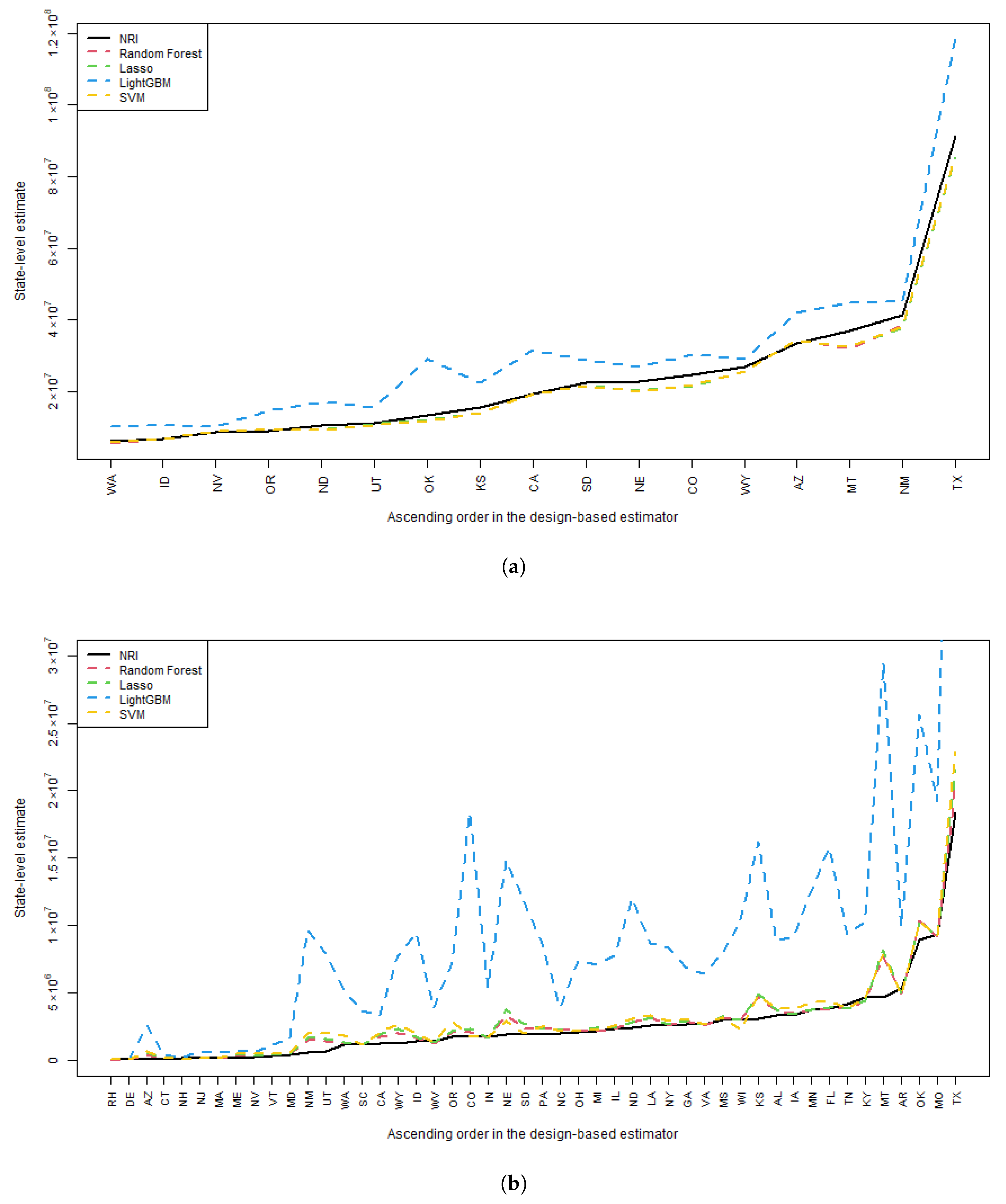
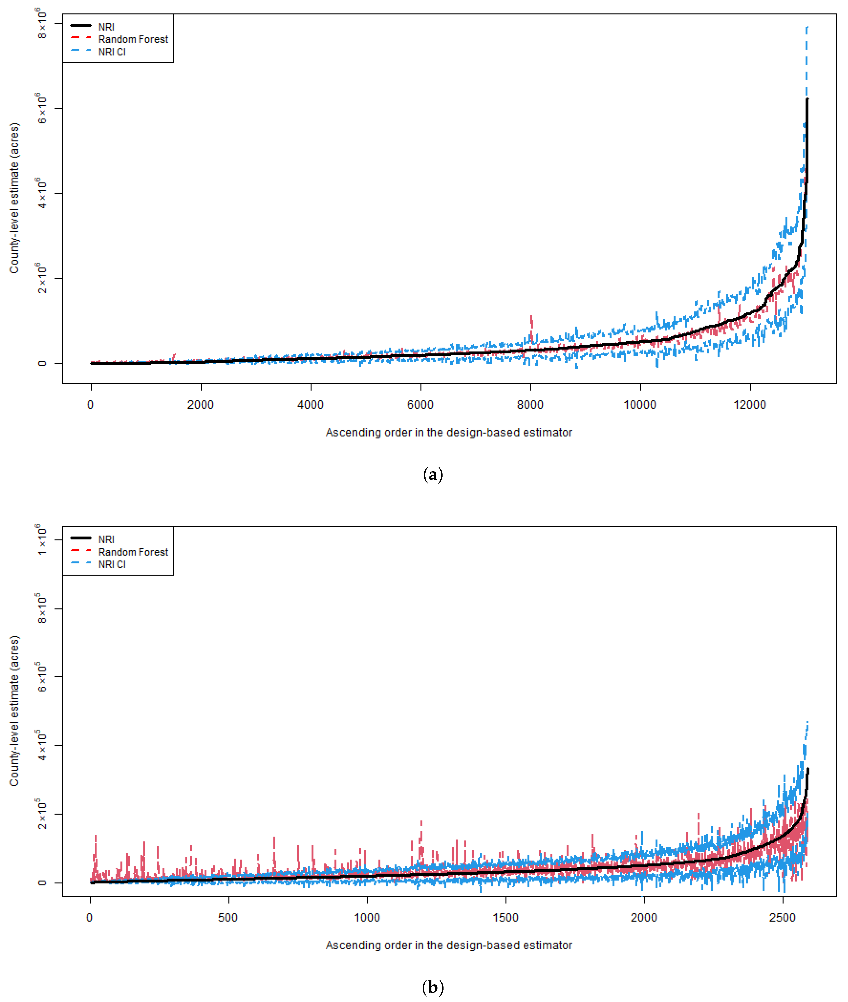
Figure 12a compares NRI design-based estimates with model-based estimates of rangeland acreage across 17 U.S. states, ordered in ascending magnitude based on the NRI design-based estimates. The Random Forest, LASSO, and SVM models exhibit strong concordance with the design-based values, underscoring their accuracy and effectiveness in estimating rangeland acreage. In contrast, the LightGBM model displays a systematic tendency to overestimate rangeland extent. These patterns are consistent with the cross-entropy results reported in Figure 6, where Random Forest achieves the lowest median loss and the most stable distribution across states, followed by LASSO and SVM, while LightGBM exhibits substantially higher and more variable cross-entropy values. These findings suggest that Random Forest, LASSO, and SVM provide particularly reliable estimates at the state level.
Figure 12b presents a similar comparison for pastureland acreage across 48 U.S. states. Again, the Random Forest, LASSO, and SVM models align closely with the design-based estimates, indicating robust predictive performance. Conversely, the LightGBM model consistently overestimates pastureland acreage. This comparative analysis reinforces the suitability of Random Forest, LASSO, and SVM for accurate state-level pastureland estimation.

3.2. Level III Ecoregion Estimation of Total Rangeland and Pastureland Area

Building on the preceding state-level analyses, we extend our modeling framework to the EPA Level III ecoregion scale, which constitutes the primary objective of this study: generating wall-to-wall spatial predictions of rangeland and pastureland acreage. For this purpose, we employ Random Forest models (identified as the most accurate in prior evaluations) using CDL data aggregated within 7 × 7 grid sections.
A key challenge at this resolution is the limited number of NRI sample points classified as rangeland in several Level III ecoregions, which hinders the reliable estimation of region-specific models. To mitigate this limitation, ecoregions with insufficient sample sizes were combined with adjacent ecoregions that yielded state-level estimates most closely aligned with NRI design-based benchmarks (Appendix B).
To evaluate the accuracy of the Level III ecoregion models, we adopted an indirect validation strategy, as NRI design-based estimates are not available at the ecoregion level. Specifically, we fitted separate Random Forest models for each Level III ecoregion, allowing for spatial heterogeneity across ecoregions, and used the resulting continuous probability map to generate county-level predictions. These model-based estimates were compared with available NRI design-based county-level estimates, providing a proxy assessment of model performance.
Figure 13a presents this comparison for rangeland acreage across counties in 17 U.S. states, including 95% confidence intervals for the design-based estimates, with variances computed using the jackknife method. The results indicate strong alignment between model-based and design-based estimates, with estimates based on Random Forest models mostly falling within the 95% confidence intervals for the design-based estimates, demonstrating high predictive accuracy.
For pastureland estimation, we similarly transitioned from state-level to Level III Ecoregion modeling, again utilizing the Random Forest approach and 7 × 7 grid-aggregated CDL data. One exception was Level III Ecoregion 79 (Madrean Archipelago [40]), where the scarcity of NRI observations classified as pastureland impeded reliable model fitting. To address this issue, Ecoregion 79 was merged with the adjacent Ecoregion 81 (Sonoran Basin and Range [40]), selected based on consistency with state-level design-based estimates. Figure 13b presents the county-level comparison for pastureland acreage across 48 U.S. states. As with the rangeland analysis, model-based predictions were generated using ecoregion-specific Random Forest models and benchmarked against NRI county-level estimates. Confidence intervals for the design-based estimates were again calculated using the jackknife method.
The model-based estimates demonstrate strong consistency with design-based estimates in counties with large number of acres of pastureland. Divergences are largely restricted to instances where the number of NRI sample points is small. In these scenarios of limited sample size, the design-based estimates themselves become unstable and less reliable as a benchmark. Consequently, the overall high level of agreement confirms the Random Forest framework as a robust and effective approach for generating pastureland acreage estimates, particularly where design-based data are sparse.
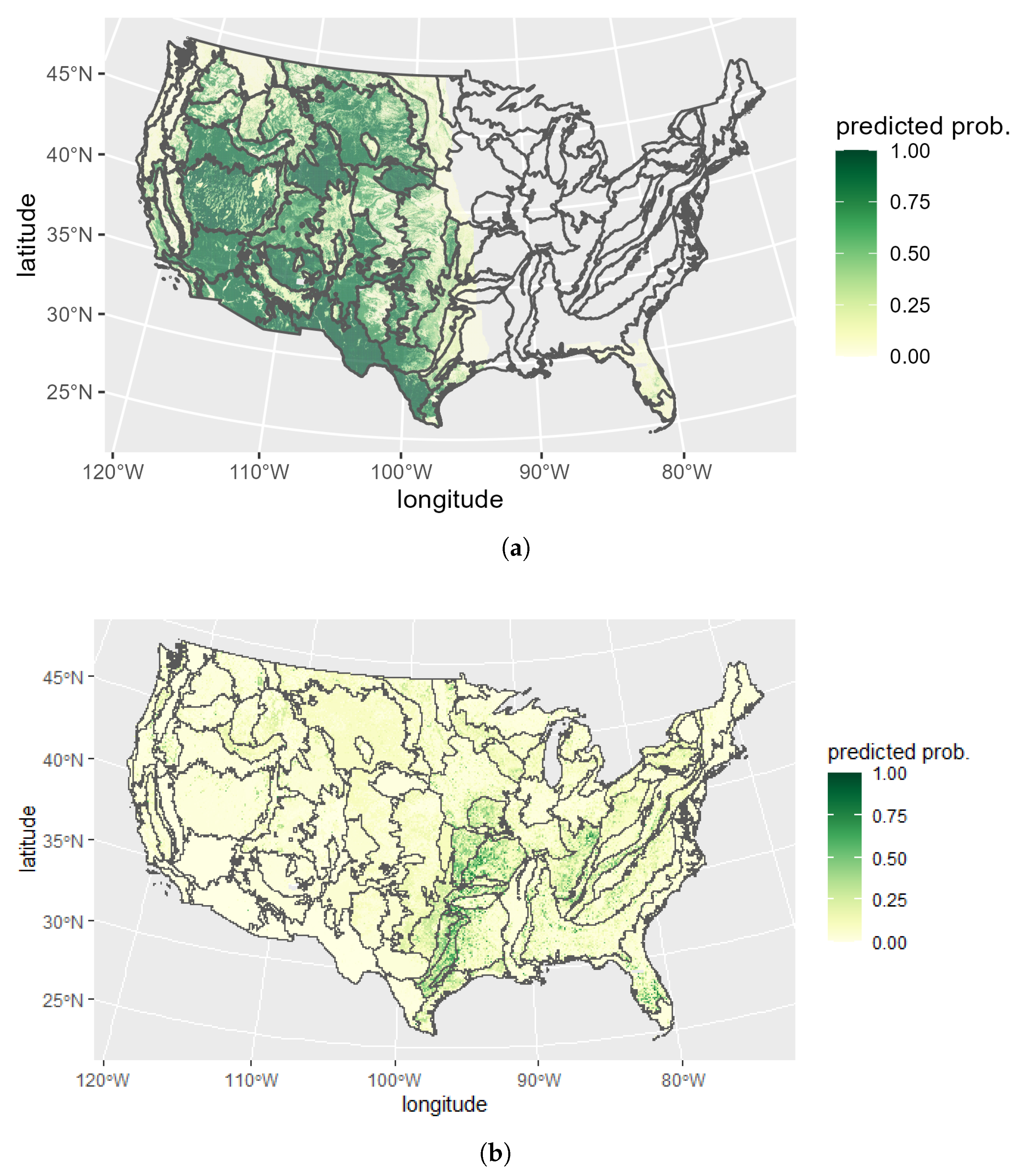
Figure 14a presents the map of predicted rangeland probability across the 17 states included in this analysis, overlaid with Level III ecoregion boundaries. Darker green shades represent areas with a higher probability of being classified as rangeland, while lighter green areas indicate lower probabilities. This probabilistic representation provides a spatial overview of rangeland distribution, facilitating the identification and extraction of specific regions of interest from which rangeland acreage can be accurately quantified. Figure 14b displays the corresponding map for pastureland, illustrating predicted probabilities across 48 states, with Level III ecoregion boundaries similarly delineated. This map offers a valuable spatial framework for assessing pastureland distribution and supports the targeted extraction of areas for accurate acreage estimation.
Furthermore, the visual contrast between Figure 14a,b highlights the substantially smaller extent of pastureland relative to rangeland, underscoring the added complexity and limitations associated with modeling and estimating pastureland acreage.
Table 7 summarizes both the NRI sample composition and the corresponding model-based rangeland acreage estimates across Level III ecoregions. After generating the map of predicted rangeland probabilities, we applied the model-based estimation procedure described in Section 2.3.1 to aggregate pixel-level predictions and obtain the estimator T ^ m for each ecoregion. These estimates represent total non-federal rangeland acreage within each Level III ecoregion and are reported in thousand acres.
The table also reports NRI Sample, the total number of NRI sample points within each ecoregion, and Range Points, the number of those points classified as rangeland. These quantities are informative not only descriptively, but also statistically, because they reveal substantial variation in class balance across ecoregions. For example, some ecoregions, such as 2 and 3, have very few rangeland-classified points relative to the total number of NRI samples, while others contain a much larger share of rangeland observations. Thus, Table 7 provides useful context for interpreting regional differences in acreage estimates and for understanding the varying difficulty of the classification task across ecological settings.
Table 8 presents Level III ecoregion-specific summaries of pastureland sample composition together with the corresponding model-based acreage estimates. After generating predicted pastureland probabilities over the spatial domain, we overlaid the prediction surface with Level III ecoregion boundaries and applied the model-based estimator described in Section 2.3.1 to obtain T ^ m for each ecoregion. The resulting values represent estimated non-federal pastureland acreage and are reported in thousand acres.
To help interpret these estimates, Table 8 also includes two sample-based quantities: NRI Sample, the total number of NRI sample points within an ecoregion, and Pasture Points, the subset of those points classified as pastureland. These counts provide additional statistical context by showing that the proportion of pastureland observations varies substantially across ecoregions. In some regions, such as 79, pastureland points account for only a small fraction of the available NRI samples, whereas in others they make up a larger share. This heterogeneity is useful for understanding regional differences in estimated pastureland extent and for assessing variation in classification difficulty across ecological settings.
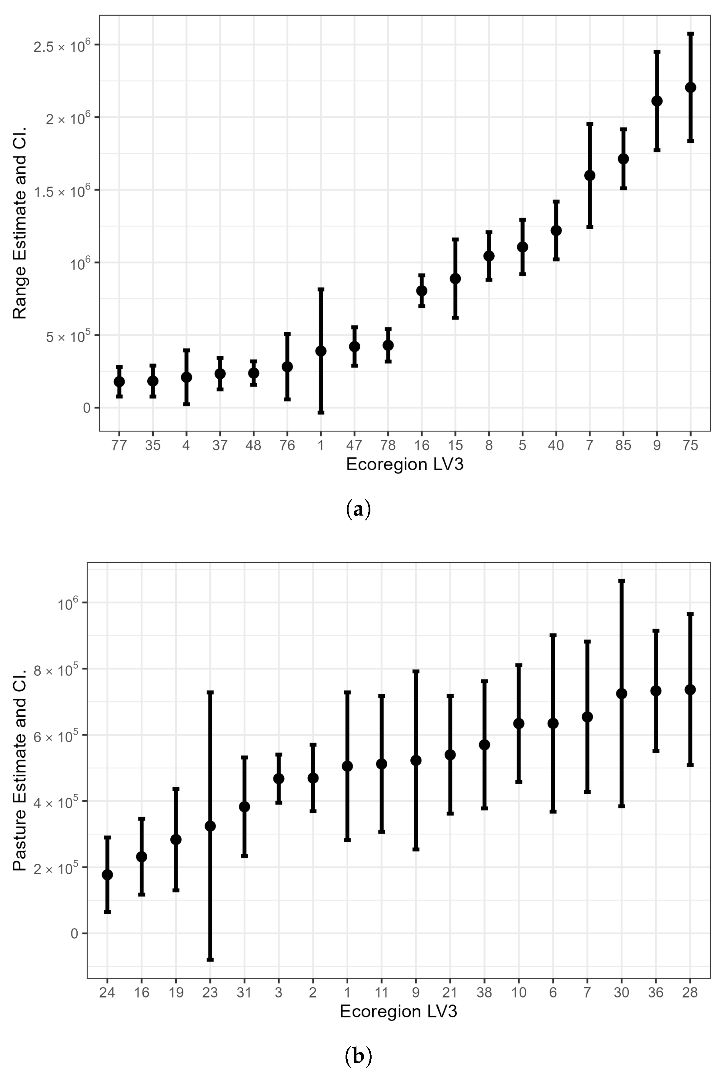
Figure 15a presents model-based rangeland acreage estimates for a selected set of Level III ecoregions, together with their corresponding 95 % confidence intervals. After obtaining the estimator T ^ m for each ecoregion, we applied the variance estimation procedure described in Section 2.3.3 to compute standard errors and construct confidence intervals. The figure shows substantial regional variation not only in estimated rangeland acreage, but also in estimation uncertainty. For example, some ecoregions, such as 1 and 15, exhibit relatively wide confidence intervals, indicating greater variance in the acreage estimates, whereas others, such as 35, 37, and 48, have comparatively narrow intervals and thus more stable estimates. Several high-acreage ecoregions, including 9 and 75, also show noticeable uncertainty, although their confidence intervals remain informative relative to the magnitude of the estimates.
Figure 15b similarly displays pastureland acreage estimates and 95 % confidence intervals for a subset of Level III ecoregions. As in panel (a), both the estimated acreage and the width of the intervals vary across regions. Some ecoregions, such as 23 and 30, show relatively large confidence intervals, suggesting higher estimation variance, while others, including 2, 3, and 19, have narrower intervals that reflect more stable pastureland estimates. These differences indicate that uncertainty is not determined solely by the magnitude of the acreage estimate, but also by regional variation in sample support and spatial heterogeneity.
These figures are intended as illustrative examples rather than a complete presentation of all Level III ecoregions. The selected ecoregions were drawn from different geographic parts of the United States and include regions with comparable estimated acreage levels, making it easier to compare uncertainty patterns across space and between rangeland and pastureland. In both panels, narrower confidence intervals indicate more precise estimates, whereas wider intervals reflect greater uncertainty. Variance estimates shown in Figure 15 were obtained using the Jackknife resampling procedure.

4. Discussion

In this study, we developed robust model-based estimators by integrating NRI survey data with CDL auxiliary data to estimate the total area of rangeland and pastureland across Level III ecoregions. Unlike traditional approaches that rely on sampling weights and predefined sampling units, our method employs a fine grid of square tiles to aggregate CDL information and use it and machine learning algorithm to predict probability of rangeland/pastureland on a fine grid, enabling flexible application to arbitrary target regions and reducing dependence on specific NRI sampling units within the target regions.
The superior performance of the 7 × 7 pixel tile may partially reflect the impact of spatial registration uncertainty between the NRI survey points and the satellite-derived CDL imagery. Although the NRI sample points are georeferenced, small positional errors may occur due to GPS uncertainty, image geolocation error, or differences between the reference coordinate systems used in the survey and the remote sensing products. When a single pixel is used as the predictor, such positional mismatch may result in the sampled pixel not accurately representing the true land cover at the NRI point. Using a larger tile aggregates information from neighboring pixels and therefore reduces the influence of these spatial registration errors. The 7 × 7 tile may provide a balance between capturing sufficient local spatial context and avoiding the inclusion of excessive surrounding heterogeneity.
In the proposed framework, the CDL is treated as an auxiliary source of information rather than as a direct land cover label. As a result, the method does not require the CDL to be perfectly accurate at the pixel level. Instead of directly using a single CDL pixel classification, we use the proportions of different CDL land cover categories within a spatial tile as predictors in the model. These aggregated category percentages capture the local land cover composition surrounding each NRI sample point and reduce the influence of individual pixel misclassification. More importantly, the regression or machine learning model is trained using the NRI photo-interpretation data as the response variable, while the CDL-derived variables enter the model as predictors. This formulation allows the model to learn systematic relationships between the CDL-derived features and the true land cover labels, which can partially offset classification errors or systematic biases present in the CDL.
By employing LASSO, Random Forest, LGBM, and SVM models, our empirical analysis revealed that the Random Forest model consistently delivered superior prediction accuracy. This was validated through the use of the AUC metric, which demonstrated the model’s effectiveness in classifying rangeland and pastureland areas with high precision. Additionally, the Random Forest model exhibited relatively small biases compared to the other approaches, further reinforcing its reliability for accurate acreage estimation. These findings suggest that the Random Forest model offers a robust and dependable solution for land area estimation in varying ecoregions.
Beyond acreage estimation, the proposed framework offers two key advances. First, it generates a probabilistic grazing land data layer that enables policymakers and researchers to identify grazing lands across the United States in a consistent and spatially explicit manner. Second, this probabilistic representation supports the estimation and assessment of grazing land conditions for custom areas of interest, allowing analyses of grazing land condition to be conducted across multiple spatial scales and inference contexts.
Although alternative land-cover products such as NLCD, ESA WorldCover, and Dynamic World may provide useful external context, direct comparison with such products is not straightforward in the present study because their thematic definitions do not exactly match the NRI-based definitions of rangeland and pastureland used here. Accordingly, model comparison in this study is focused on internal evaluation across candidate classifiers and tile sizes, together with consistency checks against NRI-based benchmark estimates.
It is important to note that, for pastureland, agreement between the model-based and design-based estimates is not as strong as that observed for rangeland, largely reflecting the substantially smaller number of NRI sample points classified as pastureland in some ecoregions. Nevertheless, the estimates exhibit a reasonable degree of consistency, suggesting that the proposed model provides a viable alternative for pastureland area estimation.
Moreover, the flexibility of our approach allows it to be applied beyond traditional state/county or Level III ecoregion boundaries, making it suitable for a wide range of user-defined geographic areas. By leveraging the grid-based CDL data aggregation, this method can be easily adapted to estimate land areas for any user-defined region, regardless of predefined administrative or ecological boundaries. Further research could explore additional applications in ecological assessments and build upon the methodological framework presented here, potentially expanding its utility for various environmental and resource management scenarios.
In addition, while the proposed framework demonstrates strong performance using CDL-derived auxiliary predictors, the current study was designed specifically to evaluate the effectiveness of CDL-based information within the modeling framework. As such, the integration of additional environmental covariates and other remote sensing products was beyond the scope of the present analysis. We acknowledge that prediction challenges may vary across geographic regions because of differences in climate, vegetation, land management context, and the quality of auxiliary predictor information. Although the pastureland and rangeland response classes used in this study are based on NRI land-use/land-cover definitions, which provide a consistent classification target across regions, geographic heterogeneity may still influence how these classes are represented in the predictor space and, consequently, affect prediction difficulty and model performance. We also note that the current framework does not explicitly distinguish among specific grassland management uses, such as mowing without grazing versus mowing combined with grazing, because the analysis relies on expert-identified reference classifications for pastureland and rangeland rather than time-series information on vegetation dynamics. Future research could improve model robustness and provide a richer characterization of grazing land patterns by incorporating additional environmental covariates, such as topographic factors (elevation, slope, and terrain indices) and climatic variables (precipitation, temperature, and aridity indices), as well as remote sensing time series and temporal indicators such as NDVI and EVI. Exploring how these additional predictors contribute to prediction accuracy and robustness across diverse geographic settings represents a promising direction for future research.
In this study, we employ class probability to estimate total rangeland and pastureland area, which offers a key advantage over traditional threshold-based classification. Specifically, by integrating predicted probabilities rather than applying an arbitrary cutoff, this approach reduces the potential bias introduced by threshold selection and yields more robust and continuous estimates of land cover extent. This differs fundamentally from the classification-based maps in [11] by providing greater flexibility for users to identify grazing lands in a manner appropriate to a given application(e.g., clipping other maps to grazing land extent for regional analysis).
The proposed framework is designed to support point-based inference by leveraging segment-level information from the CDL, and it is developed and validated using NRI observations, which provide rangeland and pastureland classifications for non-federal lands. Consequently, model estimation and validation are restricted to non-federal areas. Nevertheless, it is reasonable to apply the model estimated using data from non-federal to federal areas in the same ecoregion as they have similar landcover features, and the resulting probabilistic grazing land layer has broader potential applications beyond direct acreage estimation. For example, it may be used to delineate grazing land extents for subsetting or masking other spatial datasets—such as remote sensing imagery—thereby enabling grazing land–focused analyses across a range of environmental and management contexts. While additional data would be required to extend formal validation to federal lands, the flexibility of the framework supports its use as a general spatial tool for identifying grazing lands and facilitating multi-scale analysis.

5. Conclusions

This research provides a robust framework for estimating rangeland and pastureland acreages, allowing for expanded application of the NRI data to conservation, modeling, and ecological uses. Prior to this method, the NRI data had limited use and application in many grazingland studies because the scales of interpretation, reporting and conservation application were too coarse. With the new ability to create acreage estimates for user-defined geographies, the data is wholly relevant and useful for applications such as watershed planning, hazard estimation and risk reduction targeting, conservation planning within ecologically relevant regions, and quantifying trends in land use change, invasive species expansion, forage production variability, potential threats from increases in bare ground or other indicators, and spatiotemporal shifts in soil, water, air, plant and animal resource concerns on non-federal rangelands and pasturelands.
The findings clearly demonstrate the utility of integrating survey data with high-resolution satellite-based auxiliary data in small-area estimation. By employing methods such as Random Forest and Light GBM, the study highlights the potential of advanced computational approaches to overcome traditional challenges like small sample sizes and the high-dimensional nature of auxiliary variables. This contribution enriches the toolbox available for ecological modeling and resource management.
Although the proposed framework is flexible and applicable to user-defined geographic domains, reliable inference depends on the availability of sufficient NRI sample support within the domain of interest. Domains containing very few NRI observations—particularly for pastureland—may yield less stable estimates and higher uncertainty, and results from such areas should be interpreted with caution. In practice, users should consider minimum sample size thresholds and examine accompanying uncertainty measures when applying the model to small or highly heterogeneous regions. More generally, while the framework reduces dependence on predefined sampling units, its performance remains influenced by the spatial distribution of NRI points and the representativeness of CDL-derived predictors. These considerations highlight the importance of pairing flexible spatial aggregation with careful interpretation, especially when extending the framework to novel applications or finer spatial scales. In addition, the framework was evaluated using data from a single time period, and model performance across different years was not examined. Therefore, the temporal generalization of the proposed approach remains uncertain. The current analysis also relied only on CDL-derived predictors and did not incorporate other environmental variables, such as elevation, climate, or spectral indices, which may provide useful complementary information for grazing-land classification and acreage estimation. Future work could address these limitations by evaluating the framework across multiple years and by integrating a broader set of environmental predictors.
From a managerial perspective, the framework introduced in this study offers practical implications for land management and policymaking. The ability to generate accurate and region-specific estimates of rangeland and pastureland provides valuable insights for conservation planning, resource allocation, and assessment of grazing lands mentioned above. By moving beyond predefined administrative boundaries and adopting ecologically relevant ecoregion-level analyses, this approach ensures that land management strategies are aligned with natural resource distributions. These advancements support informed decision-making processes for stakeholders in agriculture, conservation, and environmental management.

Author Contributions

Conceptualization, M.H., C.Y., Z.Z., S.M. and L.J.M.; methodology, M.H., C.Y. and Z.Z.; formal analysis, M.H.; writing—original draft preparation, M.H., S.M., C.Y., Z.Z. and L.J.M.; writing—review and editing, M.H., C.Y., Z.Z., S.M. and L.J.M.; supervision, C.Y. and Z.Z.; funding acquisition, C.Y., Z.Z. and L.J.M. All authors have read and agreed to the published version of the manuscript.

Funding

The research was funded by USDA NRCS Conservation Effects Assessment Project-Grazing Lands (CEAP-GL), under Agreement Number NR193A750023C017.

Institutional Review Board Statement

Not applicable.

Informed Consent Statement

Not applicable.

Data Availability Statement

A GitHub repository (https://github.com/Mingyue-Hu-code/CDL, accessed on 25 March 2026) provides the code used in this study. Restricted NRI microdata are confidential and not publicly available, and therefore are not shared in the repository.

Conflicts of Interest

The authors declare no conflicts of interest.

Appendix A. Spatial Construction of CDL-Based Predictors and Tile Size Design

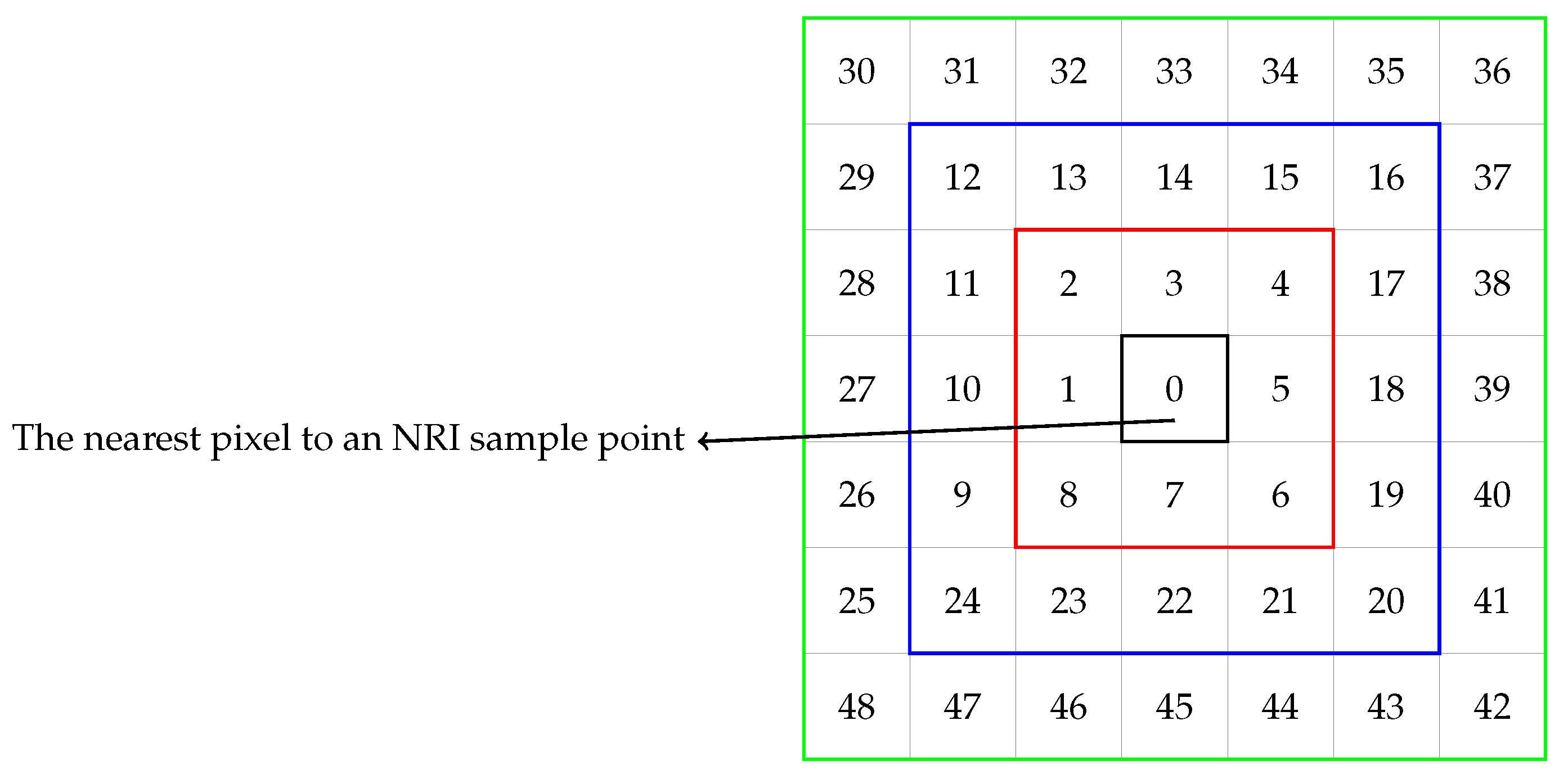
To construct the statistical model, we extracted data from 1 × 1 , 3 × 3 , 5 × 5 , and 7 × 7 square tiles of CDL pixels centered on the pixel closest to each NRI sample point (Figure A1), following the spatial sampling framework developed in Jang et al. [28]. For each tile, the CDL category of every constituent pixel was identified and recorded. The numbers shown in Figure A1 represent the pixel ID assigned to each location, with lower ID values corresponding to pixels located closer to the NRI sample point. Although the pixel ID itself was not used as a predictor in the model, this indexing structure played an important role in organizing and preserving the spatial configuration of CDL data relative to each NRI point. This consistent spatial referencing facilitated the aggregation of pixel-level information and enabled a systematic evaluation of model performance across alternative tile sizes. Overall, this approach ensured that the spatial context surrounding each sample point was uniformly captured and incorporated into the modeling framework.
Investigating the impact of different square tile sizes on model performance is essential for optimizing predictive accuracy. Smaller square tiles tend to capture more localized information at NRI sample locations; however, tiles that are too small may yield insufficient data, thereby increasing estimator variability. Conversely, larger square tiles may incorporate extraneous land-cover information, potentially introducing bias into the estimators. To explore this trade-off, we conducted a comparative analysis using South Dakota and Arkansas data, evaluating square tile sizes of 1 × 1 , 3 × 3 , 5 × 5 , and 7 × 7 .
To extract usable information from the CDL data, we compute the proportion of pixels belonging to each specific category and utilize this information to estimate the acres of rangeland/pastureland in regions of interest. Given that the CDL encompasses 169 distinct categories, employing machine learning methods, provides significant advantages. Traditional statistical methods may struggle with a large number of predictors, leading to issues such as overfitting and inefficiency. Machine learning techniques, on the other hand, are specifically designed to handle large numbers of variables, enabling more robust feature selection and improved predictive accuracy. This approach enhances our ability to accurately estimate rangeland and pastureland in the areas of interest
Figure A1. The sequence numbers of observations are derived from a 7 × 7 grid of pixels centered on the pixel closest to an NRI sample point. The boundaries of the different tile sizes are as follows: the black boundary represents a 1 × 1 square tile, the red boundary indicates a 3 × 3 square tile, the blue boundary signifies a 5 × 5 square tile, and the green boundary corresponds to a 7 × 7 square tile.
Remotesensing 18 01050 g0a1

Appendix B. Handling Sparse NRI Samples at Level III Ecoregions

Some Level III ecoregions contain very few NRI sample points classified as the target land-use type, which can lead to unstable model fitting and unreliable area estimates at the ecoregion level. To address this issue, we applied a simple and reproducible merging rule for sparse ecoregions.
For the rangeland analysis, a Level III ecoregion was considered sparse if it contained fewer than three NRI sample points classified as rangeland. Only four ecoregions met this condition. For the pastureland analysis, the same rule was applied using the number of NRI sample points classified as pastureland, and only one ecoregion met this criterion. Therefore, the merging procedure affected only a small number of ecoregions in the study.
When merging was required, a sparse Level III ecoregion was merged only with an adjacent Level III ecoregion in order to preserve geographic and ecological continuity. If multiple adjacent candidates were available, we selected the ecoregion whose state-level model-based estimates showed the greatest concordance with the corresponding NRI design-based estimates. This rule was applied prior to the final ecoregion-level estimation procedure and was used only to stabilize estimation in regions with extremely limited target-class samples.
The specific ecoregion combinations used for the rangeland analysis are summarized in Table A1. Because the merging procedure was triggered only for extremely sparse ecoregions, its impact on the overall state-level results is limited.
Table A1. Level III ecoregions merged in the rangeland analysis due to extremely sparse NRI rangeland samples (fewer than three target-class points).
Sparse Eco Lv3Rangeland NRI PointsNon-Rangeland NRI PointsCombined Eco Lv3Rangeland NRI PointsNon-Rangeland NRI Points
206991521161
32711421555
380293735239
392110402071264
For pastureland, only one Level III ecoregion met the sparse-sample criterion (fewer than three NRI pastureland points), so the effect of merging on the pastureland analysis was minimal. The specific ecoregion combination used for the pastureland analysis is summarized in Table A2.
Table A2. Level III ecoregions merged in the pastureland analysis due to extremely sparse NRI pastureland samples (fewer than three target-class points).
Sparse Eco Lv3Pastureland NRI PointsNon-Pastureland NRI PointsCombined Eco Lv3Pastureland NRI PointsNon-Pastureland NRI Points
7924228141111

References

  1. Briske, D.D. Rangeland Systems: Foundation for a Conceptual Framework. In Rangeland Systems; Briske, D.D., Ed.; Springer Series on Environmental Management; Springer: Cham, Switzerland, 2017; pp. 1–21. [Google Scholar] [CrossRef]
  2. Booker, K.; Huntsinger, L.; Bartolome, J.W.; Sayre, N.F.; Stewart, W. What Can Ecological Science Tell Us about Opportunities for Carbon Sequestration on Arid Rangelands in the United States? Glob. Environ. Change 2013, 23, 240–251. [Google Scholar] [CrossRef]
  3. Sala, O.E.; Yahdjian, L.; Havstad, K.; Aguiar, M.R. Rangeland Ecosystem Services: Nature’s Supply and Humans’ Demand. In Rangeland Systems; Briske, D.D., Ed.; Springer Series on Environmental Management; Springer: Cham, Switzerland, 2017; pp. 467–489. [Google Scholar] [CrossRef]
  4. U.S. Department of Agriculture; Natural Resources Conservation Service. National Resources Inventory: Summary Report; Technical report; USDA-NRCS: Washington, DC, USA, 2022.
  5. U.S. Department of Agriculture; Natural Resources Conservation Service. National Resources Inventory (NRI) Glossary; Technical report; USDA-NRCS: Washington, DC, USA, 2022.
  6. Reeves, M.; Krebs, M.; McCord, S.E.; Fitzpatrick, M.; Claassen, R.; Kachergis, E.; Metz, L.J.; Hanberry, B.B. Rangeland Resources. In Future of America’s Forest and Rangelands; U.S. Department of Agriculture, Forest Service: Washington, DC, USA, 2023; p. pp. 8–1–8–33. [Google Scholar] [CrossRef]
  7. Veblen, K.E.; Pyke, D.A.; Aldridge, C.L.; Casazza, M.L.; Assal, T.J.; Farinha, M.A. Monitoring of Livestock Grazing Effects on Bureau of Land Management Land. Rangel. Ecol. Manag. 2014, 67, 68–77. [Google Scholar] [CrossRef]
  8. Bestelmeyer, B.T.; Utsumi, S.; McCord, S.; Browning, D.M.; Burkett, L.M.; Elias, E.; Estell, R.; Herrick, J.; James, D.; Spiegal, S.; et al. Managing an Arid Ranch in the 21st Century: New Technologies for Novel Ecosystems. Rangelands 2023, 45, 60–67. [Google Scholar] [CrossRef]
  9. Metz, L.J.; Rewa, C.A. Conservation Effects Assessment Project: Assessing Conservation Practice Effects on Grazing Lands. Rangelands 2019, 41, 227–232. [Google Scholar] [CrossRef]
  10. Spaeth, K.E.; Rutherford, W.A.; Houdeshell, C.A.; Williams, C.J.; Simpson, B.; Green, S.; Toledo, D.; Suffridge, E.; McCord, S.E. Insights from the USDA Grazing Land National Resources Inventory and Field Studies. J. Soil Water Conserv. 2024, 79, 37A–42A. [Google Scholar] [CrossRef]
  11. Reeves, M.C.; Mitchell, J.E. Extent of Coterminous U.S. Rangelands: Quantifying Implications of Differing Agency Perspectives. Rangel. Ecol. Manag. 2011, 64, 585–597. [Google Scholar] [CrossRef]
  12. Boryan, C.; Yang, Z.; Mueller, R.; Craig, M. Monitoring U.S. Agriculture: The U.S. Department of Agriculture, National Agricultural Statistics Service, Cropland Data Layer Program. Geocarto Int. 2011, 26, 341–358. [Google Scholar] [CrossRef]
  13. Nusser, S.M.; Goebel, J.J. The National Resources Inventory: A Long-Term Multi-Resource Monitoring Programme. Environ. Ecol. Stat. 1997, 4, 181–204. [Google Scholar] [CrossRef]
  14. U.S. Department of Agriculture; National Agricultural Statistics Service. Cropland Data Layer Frequently Asked Questions. 2026. Available online: https://www.nass.usda.gov/Research_and_Science/Cropland/sarsfaqs2.php (accessed on 17 March 2026).
  15. U.S. Department of Agriculture; National Agricultural Statistics Service. 2024 Cropland Data Layer Metadata. 2026. Available online: https://data.nass.usda.gov/Research_and_Science/Cropland/metadata/metadata_Cropland-Data-Layer-2024.htm (accessed on 17 March 2026).
  16. U.S. Department of Agriculture; National Agricultural Statistics Service. CropScape and Cropland Data Layer Announcements. 2026. Available online: https://www.nass.usda.gov/Research_and_Science/Cropland/SARS1a.php (accessed on 17 March 2026).
  17. U.S. Geological Survey. National Land Cover Database (NLCD) 2021 Land Cover. 2023. Available online: https://data.usgs.gov/datacatalog/data/USGS:649595d8d34ef77fcb01dca1 (accessed on 20 March 2026).
  18. Multi-Resolution Land Characteristics Consortium. National Land Cover Database Class Legend and Description. 2026. Available online: https://www.mrlc.gov/data/legends/national-land-cover-database-class-legend-and-description (accessed on 20 March 2026).
  19. European Space Agency. Worldwide Land Cover Mapping. 2026. Available online: https://esa-worldcover.org/en (accessed on 17 March 2026).
  20. Google Earth Engine. ESA WorldCover 10m v200. 2026. Available online: https://developers.google.com/earth-engine/datasets/catalog/ESA_WorldCover_v200 (accessed on 17 March 2026).
  21. Google Earth Engine. Introduction to Dynamic World (Part 1). 2022. Available online: https://developers.google.com/earth-engine/tutorials/community/introduction-to-dynamic-world-pt-1 (accessed on 17 March 2026).
  22. Google and World Resources Institute. Dynamic World: 10m Global Land Cover Dataset. 2026. Available online: https://dynamicworld.app/ (accessed on 17 March 2026).
  23. Shandu, I.D.; Xulu, S.; Gebreslasie, M. Enhancing Land Cover Classification in the Heterogeneous Landscape by Integrating Auxiliary Data with Sentinel-2 Imagery Using the Random Forest Algorithm. Front. Remote Sens. 2025, 6, 1697897. [Google Scholar] [CrossRef]
  24. Deressu, T.F.; Bojer, A.K.; Debelee, T.G.; Negera, W.G.; Nadarajah, S.; Gebissa, K.W. Enhancing Land Use and Land Cover Classification with Deep Learning-Based Satellite Imagery Segmentation. Int. J. Appl. Earth Obs. Geoinf. 2025, 141, 104839. [Google Scholar] [CrossRef]
  25. Hester, D.; Martins, V.S.; Ferreira, L.B.; Lima, T.M.A. Learning with Less: Label-Efficient Land Cover Classification with Segmentation Foundation Models. Environ. Data Sci. 2026, 13, 100397. [Google Scholar] [CrossRef]
  26. Liu, P.; Chen, Y.; Liang, X.; Li, H.; Biljecki, F.; Stouffs, R. A Graph Neural Network for Small-Area Estimation: Integrating Spatial Regularisation, Heterogeneous Spatial Units, and Bayesian Inference. Int. J. Geogr. Inf. Sci. 2025, 1–39. [Google Scholar] [CrossRef]
  27. Sainsbury-Dale, M.; Zammit-Mangion, A.; Huser, R. Neural Bayes Estimators for Irregular Spatial Data Using Graph Neural Networks. J. Comput. Graph. Stat. 2025, 34, 1153–1168. [Google Scholar] [CrossRef]
  28. Jang, D.G.; Yu, C.; Zhu, Z. Estimating Total Acres of Rangeland for Specific Geographies Using Cropland Data Layer (CDL). J. Surv. Stat. Methodol. 2025. Accepted for publication. [Google Scholar] [CrossRef]
  29. U.S. Department of Agriculture; Natural Resources Conservation Service. Acreage of Non-Federal Rangeland, 2012, 2016. Map ID: m13900_RAD. Data Source: 2012 National Resources Inventory (NRI). Available online: https://www.nrcs.usda.gov/nri (accessed on 25 March 2026).
  30. Han, W.; Yang, Z.; Di, L.; Mueller, R. CropScape: A Web Service-Based Application for Exploring and Disseminating U.S. Conterminous Geospatial Cropland Data Products for Decision Support. Comput. Electron. Agric. 2012, 84, 111–123. [Google Scholar] [CrossRef]
  31. Tibshirani, R. Regression Shrinkage and Selection via the Lasso. J. R. Stat. Soc. Ser. B 1996, 58, 267–288. [Google Scholar] [CrossRef]
  32. Ke, G.; Meng, Q.; Finley, T.; Wang, T.; Chen, W.; Ma, W.; Ye, Q.; Liu, T.Y. LightGBM: A Highly Efficient Gradient Boosting Decision Tree. In Proceedings of the Advances in Neural Information Processing Systems, Long Beach, CA, USA, 4–9 December 2017; Volume 30. [Google Scholar]
  33. Cortes, C.; Vapnik, V. Support-Vector Networks. Mach. Learn. 1995, 20, 273–297. [Google Scholar] [CrossRef]
  34. Breiman, L. Random Forests. Mach. Learn. 2001, 45, 5–32. [Google Scholar] [CrossRef]
  35. U.S. Environmental Protection Agency. 2025. Ecoregions. Available online: https://www.epa.gov/eco-research/ecoregions (accessed on 25 March 2026).
  36. Omernik, J.M. Ecoregions of the Conterminous United States. Ann. Assoc. Am. Geogr. 1987, 77, 118–125. [Google Scholar] [CrossRef]
  37. U.S. Environmental Protection Agency. Level III Ecoregions of the United States; U.S. Environmental Protection Agency: Washington, DC, USA, 2013.
  38. U.S. Department of Agriculture; Natural Resources Conservation Service. National Resources Inventory: A Guide for Users and Summary of Methodology; Technical report; USDA-NRCS: Washington, DC, USA, 2018.
  39. Shao, J.; Tu, D. The Jackknife and Bootstrap; Springer: New York, NY, USA, 1995; pp. 27–41. [Google Scholar] [CrossRef]
  40. U.S. Department of Agriculture; Forest Service. Level III Ecoregions of the Continental United States. 2013. Available online: https://www.fs.usda.gov/database/feis/plants/shrub/arttriw/Level_III_ecoregions.pdf (accessed on 25 March 2026).
Figure 1. Illustration of three stages: data processing, modeling, and estimation of grazing land extents.
Remotesensing 18 01050 g001
Figure 2. Spatial distribution of non-federal rangeland in the contiguous United States based on the USDA NRI, 2012. Yellow dots indicate rangeland locations, with each dot representing approximately 25,000 acres. Gray shaded areas denote federal lands, which are excluded from the NRI rangeland classification. This figure is reproduced from a publicly available USDA NRCS report (public-domain U.S. federal material; https://www.nrcs.usda.gov/sites/default/files/2022-10/RangelandReport2018_0.pdf, accessed on 27 March 2026).
Remotesensing 18 01050 g002
Figure 3. Spatial distribution of non-federal pastureland in the contiguous United States based on the USDA NRI, 2012. Blue dots indicate pastureland locations, with each dot representing approximately 25,000 acres. Gray shaded areas denote federal lands, which are not included in the NRI pastureland classification. This figure is reproduced from a publicly available USDA NRCS report (public-domain U.S. federal material; https://www.nrcs.usda.gov/sites/default/files/2022-10/PasturelandReport_0.pdf, accessed on 27 March 2026).
Remotesensing 18 01050 g003
Figure 4. CDL major land-cover categories in the contiguous United States. Each pixel in this map represents a 30-m × 30-m land-cover observation from CDL; colors represent major agricultural and non-agricultural land-cover categories. This figure is based on official USDA NASS CDL materials (public-domain U.S. federal material; https://www.nass.usda.gov/Research_and_Science/Cropland/sarsfaqs2.php, accessed on 27 March 2026).
Remotesensing 18 01050 g004
Figure 5. Left: Satellite imagery from Google Earth illustrating land-cover conditions in a representative area. Right: Grid-based illustration of CDL land-cover categories surrounding an illustrative NRI sample center (black dot; not an actual location). Each tile represents a 30 × 30 m CDL pixel. Within this example tile, Deciduous Forest accounts for 36.7% of pixels, followed by Grass/Pasture (34.7%), Shrubland (14.3%), Evergreen Forest (4%), Woody Wetlands (4%), Developed/Low Intensity land (4%), and Mixed Forest (2%); all remaining land-cover categories have zero share. These pixel proportions form the covariate vector X used in the model, while the center location provides the binary response indicator Y (e.g., pastureland).
Remotesensing 18 01050 g005
Figure 6. Level III Ecoregions of the contiguous United States as defined by the U.S. Environmental Protection Agency (EPA). The map delineates a total of 85 Level III ecoregions, each representing areas with relatively homogeneous ecological characteristics, including climate, landform, soils, vegetation, and land use. The numeric labels correspond to the official Level III ecoregion codes used by the EPA and are referenced throughout the analysis to summarize rangeland and pastureland estimates by ecological region. This figure is based on publicly available EPA ecoregion materials (public-domain U.S. federal material; https://www.epa.gov/eco-research/ecoregions, accessed on 27 March 2026).
Remotesensing 18 01050 g006
Figure 7. An illustration of a grid overlaid on a target area. The polygon delineates the area of interest, which can be any spatial dimension (e.g., an EPA Ecoregion, a Hydrologic Unit Area, etc.). Red dots indicate NRI sample points classified as rangeland, while blue dots denote NRI sample points classified as non-rangeland. W i indicates number of pixels in CDL tile within the area of interest [28].
Remotesensing 18 01050 g007
Figure 8. Top 10 permutation-based feature importance values for the final 7 × 7 Random Forest models. Panel (a) shows the rangeland model based on South Dakota, and panel (b) shows the pastureland model based on Arkansas. The y-axis lists the CDL-derived predictor classes, and the x-axis reports permutation importance. Each importance value represents the reduction in predictive performance caused by randomly permuting the corresponding predictor while holding the remaining predictors unchanged; larger values therefore indicate greater influence on model prediction.
Remotesensing 18 01050 g008
Figure 9. Boxplots summarizing the distribution of AUC values for four classification methods (LASSO, LightGBM, Random Forest, and SVM). Panel (a) shows rangeland results based on state-level analyses across 17 states, while panel (b) shows pastureland results based on state-level analyses across the contiguous 48 states. The x-axis indicates the classification method, and the y-axis reports AUC values. Each boxplot is constructed from state-specific AUC values obtained by applying the corresponding method to classify rangeland or pastureland within each state.
Remotesensing 18 01050 g009
Figure 10. Top 10 aggregated feature importance values across the state-specific 7 × 7 Random Forest models. Panel (a) shows the rangeland results, and panel (b) shows the pastureland results. The y-axis lists the CDL-derived predictor classes, and the x-axis reports the summed feature importance across all fitted state-level models. Larger values indicate predictors that were more consistently influential in classification across states.
Remotesensing 18 01050 g010
Figure 11. Boxplots of cross-entropy loss values for (a) rangeland across 17 states and (b) pastureland across the contiguous 48 states. For each method shown on the x-axis (LASSO, LightGBM, Random Forest, and SVM), cross-entropy loss is computed at the state level using fitted class probabilities obtained from the corresponding model. Lower values indicate better probabilistic calibration.
Remotesensing 18 01050 g011
Figure 12. Estimates of (a) the rangeland area across 17 states, and (b) the pastureland area across 48 states, compared among the machine learning models and the NRI design-based approach. States are ordered in ascending amounts of rangeland/pastureland acres based on the NRI design-based approach.
Remotesensing 18 01050 g012
Figure 13. County-level Random Forest estimates of (a) rangeland acreage across 17 U.S. states and (b) pastureland acreage across 48 U.S. states, compared with NRI design-based estimates and their corresponding 95% confidence intervals. Counties are ordered in ascending magnitude of rangeland or pastureland acreage based on the NRI design-based estimates.
Remotesensing 18 01050 g013
Figure 14. Spatial distribution of model-predicted probabilities overlaid with Level III ecoregion boundaries for (a) rangeland and (b) pastureland in the contiguous United States. Darker green indicates a higher predicted probability p ^ . Point-level predicted probabilities and coordinates are available as CSV files on GitHub (https://github.com/Mingyue-Hu-code/CDL, accessed on 25 March 2026).
Remotesensing 18 01050 g014
Figure 15. (a) Rangeland Level III Ecoregions Estimates and Confidence Interval; (b) Pastureland Level III Ecoregions Estimates and Confidence Interval.
Remotesensing 18 01050 g015
Table 1. Comparison of candidate auxiliary land-cover products for grazing-land applications.
Data SourceResolutionCoveragePasture/Rangeland Indicator
CDL30 m 1U.S.Partial pastureland; no explicit rangeland
NLCD30 mU.S.Broad grassland/herbaceous and pasture/hay; no explicit rangeland
ESA WorldCover10 mGlobalNo explicit pastureland or rangeland
Dynamic World10 mGlobalIndirect pastureland; no explicit rangeland
1 CDL is 30 m for 2008–2023 and 10 m beginning in 2024.
Table 2. Counts of 2017 NRI point-level observations and the subset classified as rangeland across seventeen states.
StateTotal NRI PointsRangeland Points
Arizona16161127
California59711999
Colorado48262040
Idaho45001584
Kansas58161495
Montana43141712
Nebraska50971363
Nevada16381199
New Mexico34342209
North Dakota58981215
Oklahoma44471238
Oregon3709923
South Dakota52491802
Texas13,6705623
Utah1826821
Washington3789559
Wyoming26291673
Table 3. Counts of 2017 NRI point-level observations and the subset classified as pastureland across 48 states.
StateTotal NRI PointsPasture PointsStateTotal NRI PointsPasture Points
Alabama4048524Nebraska5097321
Arizona161619Nevada163857
Arkansas3625497New Hampshire144425
California5971222New Jersey158260
Colorado4826251New Mexico3434156
Connecticut127547New York4701440
Delaware83929North Carolina4432307
Florida5532580North Dakota5898399
Georgia4592345Ohio4673414
Idaho4500457Oklahoma44471061
Illinois6413472Oregon3709366
Indiana4365342Pennsylvania5056454
Iowa5117590Rhode Island80621
Kansas5816565South Carolina3473195
Kentucky4127761South Dakota5249254
Louisiana3917482Tennessee4274677
Maine156443Texas13,6701902
Maryland2830205Utah1826216
Massachusetts172445Vermont1553136
Michigan6051414Virginia4935484
Minnesota6831585Washington3789226
Mississippi4796543West Virginia2339254
Missouri61671335Wisconsin5340507
Montana4314524Wyoming2629224
Table 4. AUC values for combinations of method and CDL tile resolution when predicting rangeland (South Dakota) and pastureland (Arkansas). Each row corresponds to a specific land-cover class and tile size, while columns report AUC values for four modeling approaches. Higher AUC values indicate stronger discriminatory performance. For each land-cover class, the highest AUC across all methods and resolutions is highlighted in bold.
ClassTile SizeLightGBMSVMRandom ForestLASSOmin
Rangeland 1 × 1 0.91340.89700.91330.9143
Rangeland 3 × 3 0.94200.94280.94410.9446
Rangeland 5 × 5 0.94680.94680.94880.9485
Rangeland 7 × 7 0.94670.94850.95100.9507
Pastureland 1 × 1 0.90490.87250.90700.9050
Pastureland 3 × 3 0.93550.91150.93880.9348
Pastureland 5 × 5 0.93770.91140.93920.9342
Pastureland 7 × 7 0.93880.91600.94100.9331
Table 5. AUC values obtained using leave-county-out spatial cross-validation for combinations of method and CDL tile resolution when predicting rangeland (South Dakota) and pastureland (Arkansas). For each land-cover class, the highest AUC across all methods and resolutions is highlighted in bold.
ClassTile SizeLightGBMSVMRandom ForestLASSOmin
Rangeland 1 × 1 0.91140.88110.91120.9123
Rangeland 3 × 3 0.94020.94140.94260.9429
Rangeland 5 × 5 0.94500.94530.94720.9452
Rangeland 7 × 7 0.94550.94750.94910.9478
Pastureland 1 × 1 0.89590.83470.89700.8992
Pastureland 3 × 3 0.93200.90980.93880.9342
Pastureland 5 × 5 0.93800.91150.93900.9354
Pastureland 7 × 7 0.93900.91620.94050.9341
Table 6. Cross-entropy loss values for combinations of method and CDL tile resolution when predicting rangeland (South Dakota) and pastureland (Arkansas). Each row corresponds to a specific land-cover class and tile size, while columns report cross-entropy values for four modeling approaches. Lower cross-entropy values indicate better probabilistic calibration. For each land-cover class, the lowest cross-entropy across all methods and resolutions is highlighted in bold.
ClassTile SizeLightGBMSVMRandom ForestLASSOmin
Rangeland 1 × 1 0.19570.18370.17800.1735
Rangeland 3 × 3 0.18510.19050.16800.1701
Rangeland 5 × 5 0.18020.18760.16300.1708
Rangeland 7 × 7 0.17780.18750.16090.1701
Pastureland 1 × 1 0.32880.24630.22550.2210
Pastureland 3 × 3 0.26580.21930.19550.2008
Pastureland 5 × 5 0.24630.22030.19470.2025
Pastureland 7 × 7 0.23830.22320.19680.2071
Table 7. NRI sample sizes and rangeland-classified points by Level III Ecoregions (Eco), with rangeland acreage estimates (thousand acres) included.
EcoNRI SampleRange PointsRangeland AcresEcoNRI SampleRange PointsRangeland Acres
1116352378285683303863
26990942921577928488
37132473075551514,324
457621222311579138311,588
5452847743210352182261
6169069574183313943533270
7137312815083423389856567
81219987235178727336
96831881606361396194
10212161864403727435614
11817351461438290205
12193552625003911222671
132233125611,4034014712072848
1470150847544151670
1593469830424114121414,107
16279101600434912265850,144
17158368162014444433112,083
18146395112,4114647945953702
19523242215147215466463
20129672582474863237224
21185376573487715613138
22130286623,2067869247365
234152456473794243425813
24129491725,65480171911256598
256973227426,00481111564410,985
263085210736,216854781661589
276542199623,014
Table 8. NRI sample sizes, pastureland-classified points, and model-based pastureland acreage estimates (thousand acres) by Level III Ecoregions (Eco).
EcoNRI SamplePasture PointsPastureland AcresEcoNRI SamplePasture PointsPastureland Acres
1116399484444449232
26991055114550795314101
37131054574651654262596
45766354790838524744
545244048121681596
61690715514941725326
71373835905038441731741
81213225129953232172
96831784835218322021272
10212175588531195120753
1181766499544120341752
1219352207305529842161246
132233478955564946638923
1470139572947172435
1593485836584274183774
1627994214593533152379
17158319114726036392321386
1814635110576163631700
1952364235625126159260
20129697681632561252586
211853177439642961312821
2213026463365129311236957
2341513221664595685670
241294131406745596853536
25697342642336811001771234
26308516122056921371801064
27654253157447030234042395
285686368771511711196114
292175343007252215132978
30755355517342331741230
311579453917422662981550
3210353833747559415473569
33139450751077649015122
34311473271977156414
35423476259187869261371
36375607327942426
37570382137801719100408
3815234563811115453
39210766472478297438273
404866113470028317871961023
41514598411723499
424114255265285478974
4349124115944
Disclaimer/Publisher’s Note: The statements, opinions and data contained in all publications are solely those of the individual author(s) and contributor(s) and not of MDPI and/or the editor(s). MDPI and/or the editor(s) disclaim responsibility for any injury to people or property resulting from any ideas, methods, instructions or products referred to in the content.