Integrating Multi-Source Data to Assess Temporal Changes and Drivers of Forest Cover in the Western Margins of the Sichuan Basin

Highlights

What are the main findings?

• A 2000–2024 forest dynamics assessment at 30 m reveals a marked post-2010 forest expansion and dominant non-forest → forest transitions in the Sichuan Basin margin, consistent with the regional “decline–stagnation–recovery” trajectory.
• Multi-output Random Forest with SHAP attribution shows that forest dynamics are primarily constrained by terrain and biotic legacies (e.g., elevation and initial forest fraction), while mean climate variables play a secondary role in explaining spatial heterogeneity.

What are the implications of the main findings?

• Forest recovery in complex mountain systems should not be interpreted from climate alone; terrain context and pre-disturbance forest conditions must be explicitly modeled to avoid biased driver attribution.
• The MORF–SHAP framework provides a transferable, spatially explicit way to map driver dominance and guide restoration prioritization (where to intervene vs. where recovery is topographically self-favored).

Abstract

Mountain forests on the western edge of the Sichuan Basin are challenging to monitor at high resolution because rugged topography, cloud cover, and Landsat-7 SLC-off artifacts create data gaps, while the 2008 Wenchuan earthquake and subsequent restoration further alter vegetation dynamics. We fused Landsat 5/7/8/9 surface reflectance with MODIS MOD13Q1 using an index-then-fusion STARFM framework to reconstruct a continuous 30 m NDVI record for 2000–2024 and quantified forest fraction dynamics using annual forest/non-forest maps, transition analysis, and K-means clustering of pixel-wise NDVI trajectories. To identify dominant controls, we applied a multi-output random forest with spatial block cross-validation and SHAP attribution. The fused NDVI agrees well with MODIS across 100,000 samples (R² = 0.953; RMSE = 0.032), and the regional mean NDVI increased from 0.711 (2000) to 0.774 (2024), showing a post-2008 decline–stagnation–recovery pattern. Forest fraction rose from 48.2% to 72.9%, with accelerated gains after 2010 (+21.4%), and improving trajectories dominated (70.95%), concentrating near the Longmenshan fault zone. The driver model generalized well (micro-mean R² = 0.875), and SHAP ranked elevation (32.6%) and initial forest fraction (32.3%) above temperature and precipitation. These results provide high-resolution evidence of mountain forest change and its primary controls to support terrain-informed ecological management.

1. Introduction

Forest vegetation dynamics form the basis for assessing ecosystem resilience and the cumulative effects of natural and anthropogenic disturbances [1,2,3]. Reconstructing continuous, high-resolution NDVI records in rugged mountain landscapes remains a challenge [4,5]. These areas are characterized by steep terrain, fragmented land cover, and persistent cloud cover and sensor artifacts, severely hindering the continuity of remote sensing observations. While Landsat provides the required 30 m spatial resolution for mountain ecology, its 16-day revisit period and the SLC closure issue in later Landsat-7 satellites limit its application [6]. MODIS satellites, while providing the necessary temporal resolution, produce coarse pixels that are prone to severe mixing effects in rugged terrain [7]. Therefore, generating reliable long-term 30 m NDVI sequences is fundamental for subsequent ecological analyses.

To bridge these spatiotemporal gaps, fusion techniques—particularly STARFM and its improved version ESTARFM—have become essential tools [8]. STARFM serves as the basic framework, while ESTARFM aims to better address sub-pixel heterogeneity in complex landscapes [9,10]. Despite these methods, artifacts and scale mismatches caused by mountainous terrain still affect reconstruction accuracy [11,12,13]. In the design of spatiotemporal fusion schemes, the logical order of fusion operations and vegetation index calculations affects the fidelity of the final product. Existing studies have shown that, compared with band reflectance fusion, adopting the “indices first, fusion later” (ITB) approach can effectively curb the error amplification effect caused by nonlinear operations between bands. This study constructs a technical scheme based on exponential fusion within the STARFM framework.

Changes in mountain forests rarely follow linear paths; they are influenced by the intertwining effects of topography, climate, and human activities, typically exhibiting delayed or threshold-like recovery patterns [14,15]. Traditional linear regression analysis and year-by-year independent modeling often ignore the temporal autocorrelation of vegetation dynamics, making it difficult to characterize the lag effects and non-stationary characteristics in forest evolution and lacking a systematic and coherent understanding of long-term evolutionary trends [16,17]. Machine learning can flexibly model this nonlinearity, but standard annual models treat each time step in isolation, which is not suitable for representing the continuous evolution of trajectories. Against this backdrop, multi-output learning offers a more compelling approach by modeling responses across multiple years within a unified framework [18]. This approach combines SHAP interpretation with spatial explicit verification to more transparently and robustly assess driving factors [19].

As an ecological transition zone between the Tibetan Plateau and the Sichuan Basin, the western edge of the Sichuan Basin exhibits extreme topographic relief and significant climatic heterogeneity [20]. Its history is marked by numerous disturbances, from the 2008 Wenchuan earthquake to large-scale ecological restoration and ever-changing pressures from human activities [21,22,23]. This study reconstructed NDVI trajectories (2000–2024) at 30 m resolution using a STARFM-based exponential fusion framework and applied a spatially segmented multi-output random forest (MORF) model to analyze the driving factors of forest change. This study aims to provide new evidence for vegetation resilience in one of the world’s most ecologically vulnerable mountain margins.

2. Materials and Methods

2.1. Study Area

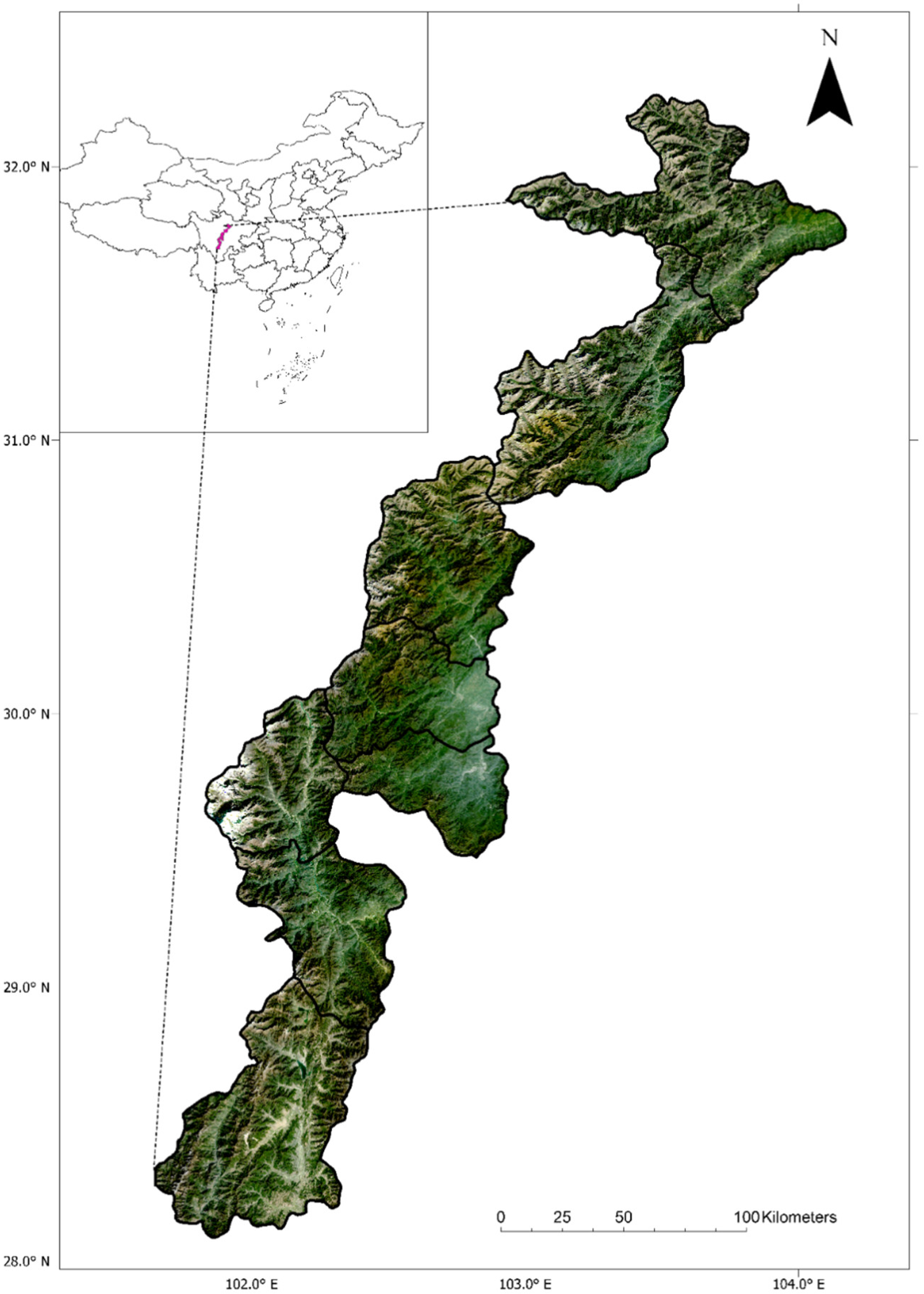
The study area is located on the western edge of the Sichuan Basin (28.4–32.4°N, 101.5–104.0°E), covering approximately 24,460.37 km² and encompassing eight counties: Maoxian, Wenchuan, Baoxing, Tianquan, Luding, Yingjing, Shimian, and Mianning (Figure 1). It is an important ecological transition zone between the western mountainous region of the Sichuan Basin and the eastern Qinghai–Tibet Plateau. Influenced by the uplift of the Qinghai–Tibet Plateau and the activity of the Longmenshan fault zone, this region has complex topography, characterized by rugged mountains and deeply incised valleys, with extreme elevation differences, ranging from a minimum of 598 m to a maximum of 7439 m.

Climatically, this region is at the intersection of plateau climate and the East Asian-Indian monsoon system, leading to substantial spatial variations in temperature and precipitation. These unique topographical and climatic conditions have fostered mountain and subalpine forest ecosystems, forming important ecological corridors. Most of these forests have experienced severe earthquake damage and are currently in a recovery phase.

2.2. Materials

2.2.1. NDVI Data

To overcome the timeliness and observational limitations of single sensors, this paper integrated four generations of Landsat satellite imagery (5/7/8/9) to construct a long-term time-series dataset from 2000 to 2024 (

Table 1. Summary of satellite data sources and characteristics. The asterisk (*) denotes datasets processed and exported via Google Earth Engine (GEE).

Data	Data Sources	Years	Spatial Resolution	Temporal Resolution
Landsat 5/7/8/9 *	USGS	2000–2011 (L5) 2012 (L7) 2013–2024 (L8, L9)	30 m	16 days
MOD13Q1 *	NASA LP DAAC	2000–2024	250 m	16 days

). Based on Collection 2 Level-2 surface reflectance products, after conversion using standard radiometric calibration coefficients, clouds, shadows, water bodies, and radiatively saturated pixels were rigorously removed using the QA_PIXEL and QA_RADSAT bands, and anomalous reflectance values were also removed. NDVI calculation results were constrained to the theoretical range of [−1, 1]; specifically, an extended time window strategy was used to fill the data gap from 2012, generating the L_NDVI dataset.

The required MODIS data (MOD13Q1) for fusion underwent quality control and reprojection, achieving strict cell-level alignment with the Landsat grid (M_NDVI). MOD13Q1 is a 16-day 250 m Level-3 vegetation index product that provides NDVI and associated quality assurance information. Finally, the STARFM algorithm was used to fuse L_NDVI and M_NDVI to reconstruct a 30 m resolution NDVI time series with full spatiotemporal coverage.

2.2.2. Climate Data

Temperature data was extracted from the ERA5-Land reanalysis dataset, while precipitation data came from the CHIRPS dataset. These datasets were spatially resampled to 30 m to match the resolution of the NDVI data.

2.2.3. Topography Data

We used the NASA SRTM Digital Elevation Model (DEM) with a spatial resolution of 30 m. Based on the DEM, we extracted elevation, slope, and aspect.

2.2.4. Population Data

We used the WorldPop gridded population density dataset. This dataset provides high-resolution population distribution estimates based on census data and machine learning methods. The population layer was resampled to 30 m (using bilinear interpolation) to align with the NDVI data.

2.2.5. Land Cover Data

Land cover information was obtained from the ESA WorldCover 2021 v200 product. This data masked non-vegetated areas. Resampling to a 30 m analysis grid and alignment with the NDVI data were performed.

2.3. Method

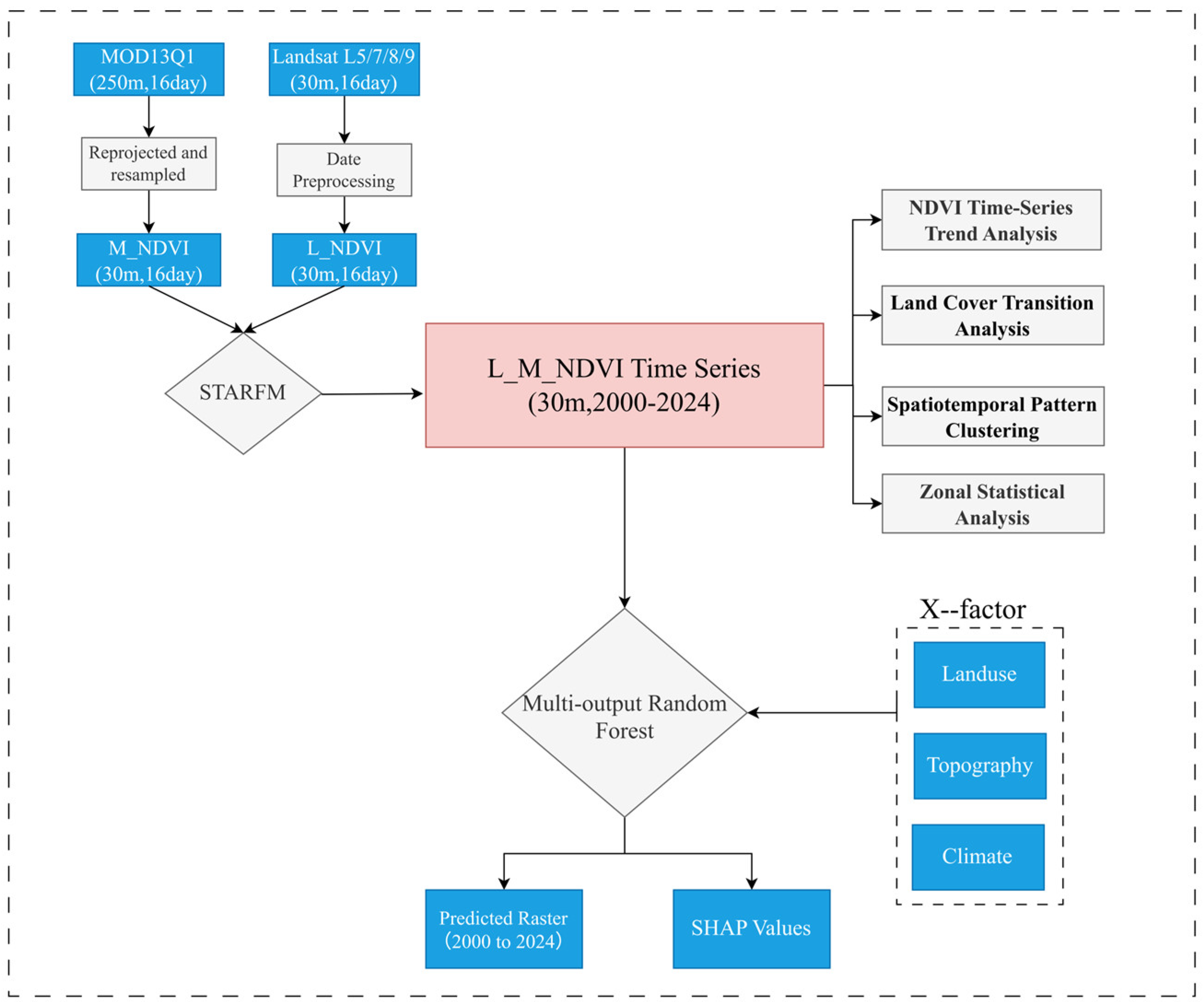
As shown in Figure 2, the methodology of this study aims to answer three interrelated questions. The first question is, can reliable 30 m resolution long-term NDVI sequences be reconstructed for cloudy and topographically complex mountainous areas? To address this, we employ the STARFM “index-then-fusion” strategy to preprocess and fuse Landsat and MODIS NDVI data, generating a continuous NDVI sequence L_M_NDVI time series from 2000 to 2024 and comparing it with benchmark products. The second question is, after obtaining the continuous sequence, how should we characterize the vegetation dynamics after disturbance? To this end, we generate annual forest/non-forest distribution maps, quantify vegetation cover changes, and use K-means clustering as a pattern description and validation layer to summarize the main NDVI change trajectories. The third question is, which environmental and anthropogenic factors best explain the observed long-term NDVI dynamics, and does the fitted model still preserve the unmodeled spatial structure? To address this, we employ a spatially segmented multi-output random forest (MORF) model, combined with SHAP-based interpretation and folded external residual spatial diagnostics. In this way, the entire workflow starts with data reconstruction, gradually transitions to trajectory recognition, and finally achieves attribution of driving factors and model validation.

2.3.1. Spatio-Temporal Fusion Model (STARFM)

To reconstruct high-frequency forest fraction dynamics in the complex terrain of the study area, we used the Spatial and Temporal Adaptive Reflectance Fusion Model (STARFM) to produce a synthetic NDVI time series with high spatial and temporal resolution. STARFM predicts the NDVI value of a central fine-resolution pixel at time $t_k$ by weighting spectrally similar pixels within a moving window, based on the linear relationship between fine-resolution (Landsat/Sentinel-2) and coarse-resolution (MODIS) data observed at a base time $t_0$ [11]. The prediction equation is given by:

$$L\left(x_i,y_j,t_k\right)=M\left(x_i,y_j,t_k\right)+w_{ijk}\times \left[L\left(x_i,y_j,t_0\right)-M\left(x_i,y_j,t_0\right)\right]$$

(1)

where $L$ and $M$ denote the NDVI values of the fine- and coarse-resolution images, respectively, and $w_{ijk}$ represents the spatial weighting function determined by spectral difference, temporal difference, and spatial distance.

Crucially, this study adopted the “Index-then-Blend” (IB) strategy, where NDVI is calculated from the original spectral bands prior to the data fusion process. We selected this strategy over the traditional “Blend-then-Index” approach (fusing bands first) based on robust evidence from previous literature. Jarihani et al. [24] demonstrated that the IB strategy effectively minimizes the error propagation that occurs when Red and NIR bands are predicted separately. Furthermore, recent adaptability evaluations by Fan et al. [13] in heterogeneous highland regions confirmed that directly fusing vegetation indices yields superior accuracy (${\mathrm{R}}^2>0.9$) and better preserves spatial details in fragmented landscapes compared to band-based fusion. This workflow has been successfully validated in similar ecological contexts for biomass estimation and long-term trend analysis [12,25], ensuring the reliability of the synthetic NDVI dataset for monitoring post-seismic forest recovery.

2.3.2. Land Cover Transition Analysis

We utilized Google Earth Engine to generate annual 30 m forest/non-forest maps from 2000 to 2024 using a random forest classifier. The classifier was trained using reference labels from the ESA WorldCover 2021 v200 product (tree cover, code 10 = forest; other = non-forest; water bodies, code 80, and permanent snow/ice, code 70, masked). Predictors included reconstructed annual NDVI (L_M_NDVI) and terrain (elevation and slope) extracted from the SRTM DEM. To improve label-feature temporal consistency and reduce single-year outliers, the NDVI predictor was defined as the average synthetic NDVI value from 2019 to 2021 (rather than single-year images). Balanced stratified sampling (3000 forest samples and 3000 non-forest samples) was employed, followed by an 80/20 training/validation split. The model was trained using 200 trees and applied to the synthetic NDVI data for each year to obtain an annual binary map. A smoothed annual forest/non-forest sequence was obtained by using a three-year sliding window majority filter to suppress temporal “flickering” (at least two of the three consecutive years being forested; boundary years were relaxed).

Transition matrices for 2000–2010, 2000–2024, and 2010–2024 were calculated using the smoothed binary maps. For each pair of years, binary maps A and B were encoded as 2A + B to classify transitions as 0 → 0 (non-forest persistence), 0 → 1 (forest increase), 1 → 0 (forest decrease), and 1 → 1 (forest persistence). The transition area (km²) was obtained by weighting pixel area and spatial aggregation within the study area; the gain/loss ratio was also calculated accordingly. The magnitude of the transitions over the three time steps was visualized using Sankey diagrams.

2.3.3. Spatiotemporal Pattern Clustering

To summarize the dominant temporal patterns of vegetation dynamics, we applied K-means clustering to the annual NDVI trajectories from 2000 to 2024 at the pixel level. For each pixel, the 25-year annual mean NDVI sequence was treated as a feature vector, and pixels were grouped by minimizing the within-cluster sum of squares. The number of clusters was set to four (k = 4) based on the elbow method and the need to retain a parsimonious yet interpretable representation of the major trajectory types in the study area. In this study, K-means was used as a trajectory-description and pattern-validation layer rather than as a predictor in the MORF model. The four clusters were named according to the temporal shape of their cluster centroids: Relatively Stable, characterized by the smallest interannual amplitude and a small difference between the beginning and end of the series; Persistently Increasing, characterized by a clearly positive start-to-end difference and an overall upward trend; Decrease-then-Increase, characterized by a pronounced mid-period trough and a V-shaped recovery pattern; and Increase-then-Decrease, characterized by an initial rise followed by a later decline, forming an inverted V-shaped trajectory.

These trajectory classes were subsequently used to examine whether the clustered NDVI patterns corresponded to meaningful environmental gradients and post-disturbance spatial signatures, rather than being merely statistical artifacts.

2.3.4. Driver Analysis Based on Multi-Output Random Forest

To analyze the underlying driving mechanisms of long-term vegetation change, we constructed a Multi-output Random Forest (MORF) regression model. Unlike building single-output models year by year, MORF treats the NDVI sequence of each pixel as a 25-dimensional response vector (2000–2024), simultaneously fitting the NDVI outputs of each year within the same framework. This allows for sharing information across different years during training and characterizing the correlation between outputs from multiple years (this method does not explicitly characterize the time dependence of the autoregressive expression).

In this framework, the response variable Y is defined as the time series of the annual mean L_M_NDVI (2000–2024). The explanatory variables X consist of anthropogenic and natural factors reflecting long-term environmental constraints, all of which are static features, including topographic factors (elevation, slope); climatic factors (multi-year average temperature and precipitation calculated based on ERA5 and CHIRPS from 2000 to 2024, used to characterize the long-term climate background); and human activities and land surface characteristics (land use/cover type or its component proportions and population density). The model is implemented using Python 3.12.7 using the scikit-learn.

To quantify the contribution of each driving factor to NDVI predictions for different years, we employ SHAP (Shapley Additive Explanations) for model interpretation. We calculate the SHAP value for each year’s output and spatially aggregate it to obtain global importance and directionality, thereby revealing the relative differences in the contribution of different factors to the NDVI series predictions for each year.

2.3.5. Spatial Residual Diagnostics of MORF

To assess whether the multi-output random forest (MORF) left unmodeled spatial structure, we analyzed out-of-fold (OOF) residual maps derived from the block cross-validation procedure. For each pixel $i$ and year $t$, the OOF residual was defined as

$$e_{i,t}=y_{i,t}-{\widehat{y}}_{i,t}^{\mathrm{OOF}}$$

(2)

where $y_{i,t}$ is the observed NDVI and ${\widehat{y}}_{i,t}^{\mathit{OOF}}$ is the prediction obtained when the pixel belonged to the validation fold. Only finite and non-nodata pixels were retained for the analysis. Global spatial autocorrelation of OOF residuals was quantified using Moran’s $\mathrm{I}$ for representative years (2007, 2008, 2010, 2012, and 2024):

$$I={\displaystyle \frac{n{\sum }_{i=1}^n{\sum }_{j=1}^n{w}_{ij}\left(e_i-\overline{e}\right)\left(e_j-\overline{e}\right)}{S_0{\sum }_{i=1}^n{\left(e_i-\overline{e}\right)}^2}}$$

(3)

where $n$ is the number of valid pixels, $e_i$ and $e_j$ are residual values at locations $i$ and $j$, $\overline{e}$ is the mean residual, $w_{ij}$ is the spatial weight between neighboring pixels, and $S_0=\sum _i\sum _j{w}_{ij}$. A rook-contiguity spatial weights matrix was constructed from the valid residual grid, isolated pixels without neighbors were removed, and row-standardized weights were used in the computation. Statistical significance was assessed using 999 random permutations and permutation-based $p$-values. Local spatial autocorrelation was further evaluated using Local Moran’s $I_i$ (LISA) for selected years (2008, 2010, and 2024):

$$I_i={\displaystyle \frac{\left(e_i-\overline{e}\right)}{m_2}}{\displaystyle \sum _{j=1}^n}{w}_{ij}\left(e_j-\overline{e}\right)$$

(4)

where

$$m_2={\displaystyle \frac{1}{n}}{\displaystyle \sum _{k=1}^n}{\left(e_k-\overline{e}\right)}^2$$

(5)

Based on 999 permutations and a significance level of α = 0.05, significant local patterns were classified into high-high (HH), low-low (LL), high-low (HL), and low-high (LH) clusters. In addition, pre- and post-earthquake residual composites were compared (2005–2007 vs. 2009–2011) to examine whether spatially structured model error intensified after the 2008 Wenchuan earthquake.

3. Results

3.1. Quality and Accuracy of the Fused 30 m NDVI Time Series

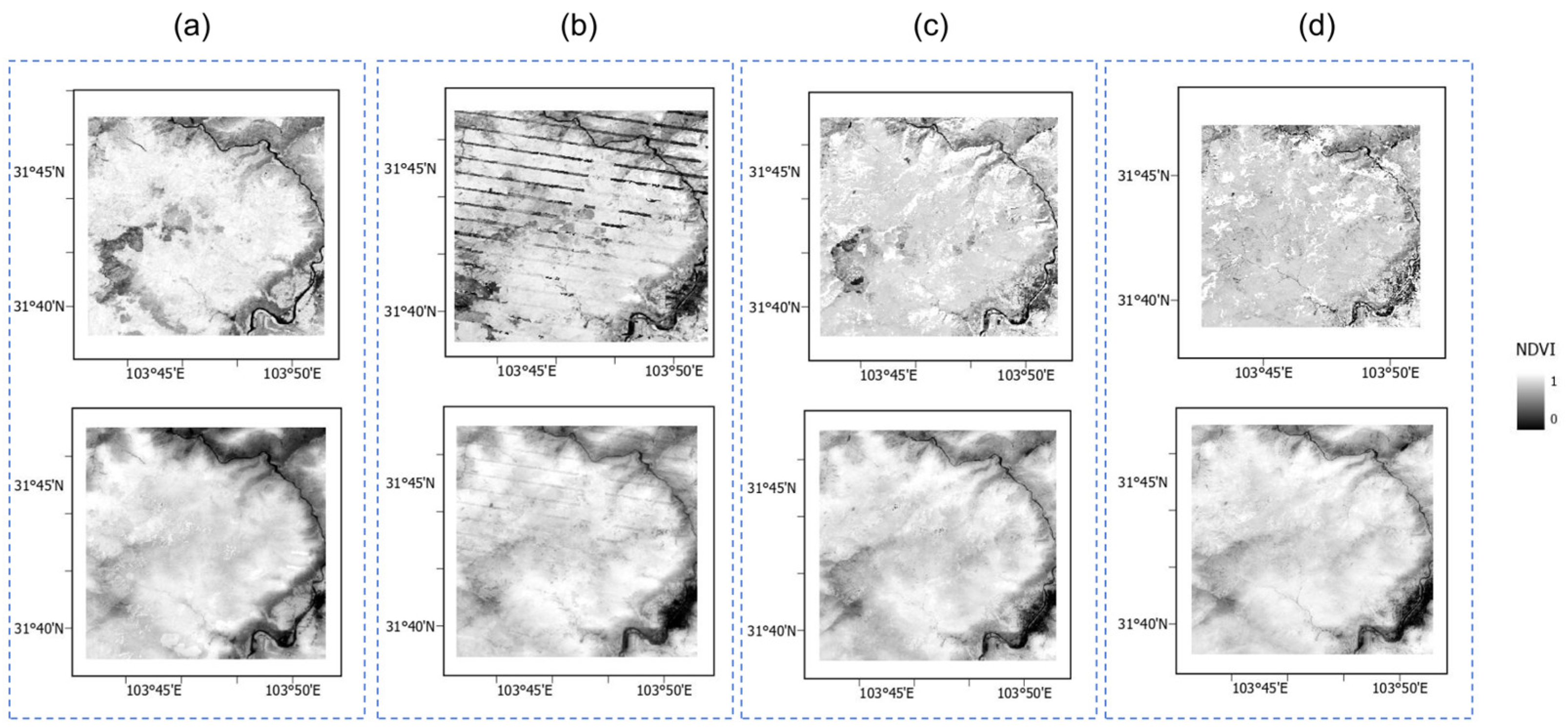
We first acquired MODIS MOD13Q1 NDVI data, performed quality control and scale factor scaling, and reprojected and resampled to a 30 m grid with strict alignment to Landsat pixels. Simultaneously, we calculated 30 m NDVI for Landsat 5/7/8/9 surface reflectance products (30 m, 16 days). Then, we combined the target period MODIS NDVI with STARFM to obtain L_M_NDVI (30 m, 16 days). Finally, we performed pixel-level compositing to generate the annual 30 m NDVI image product L_M_NDVI time series from 2000 to 2024, compensating for band gaps and cloud contamination caused by Landsat 7 SLC-OFF. Figure 3 compares local scenes from the original Landsat NDVI (top row) and the fused product (bottom row). Visual interpretation shows that the STARFM algorithm not only effectively fills in the band gaps (Figure 3) but also preserves terrain texture and boundaries. In addition, the algorithm effectively reduces the impact of cloud cover and terrain shadows. The resulting L_M_NDVI time series forms the basis for our subsequent research on trends and driving factors.

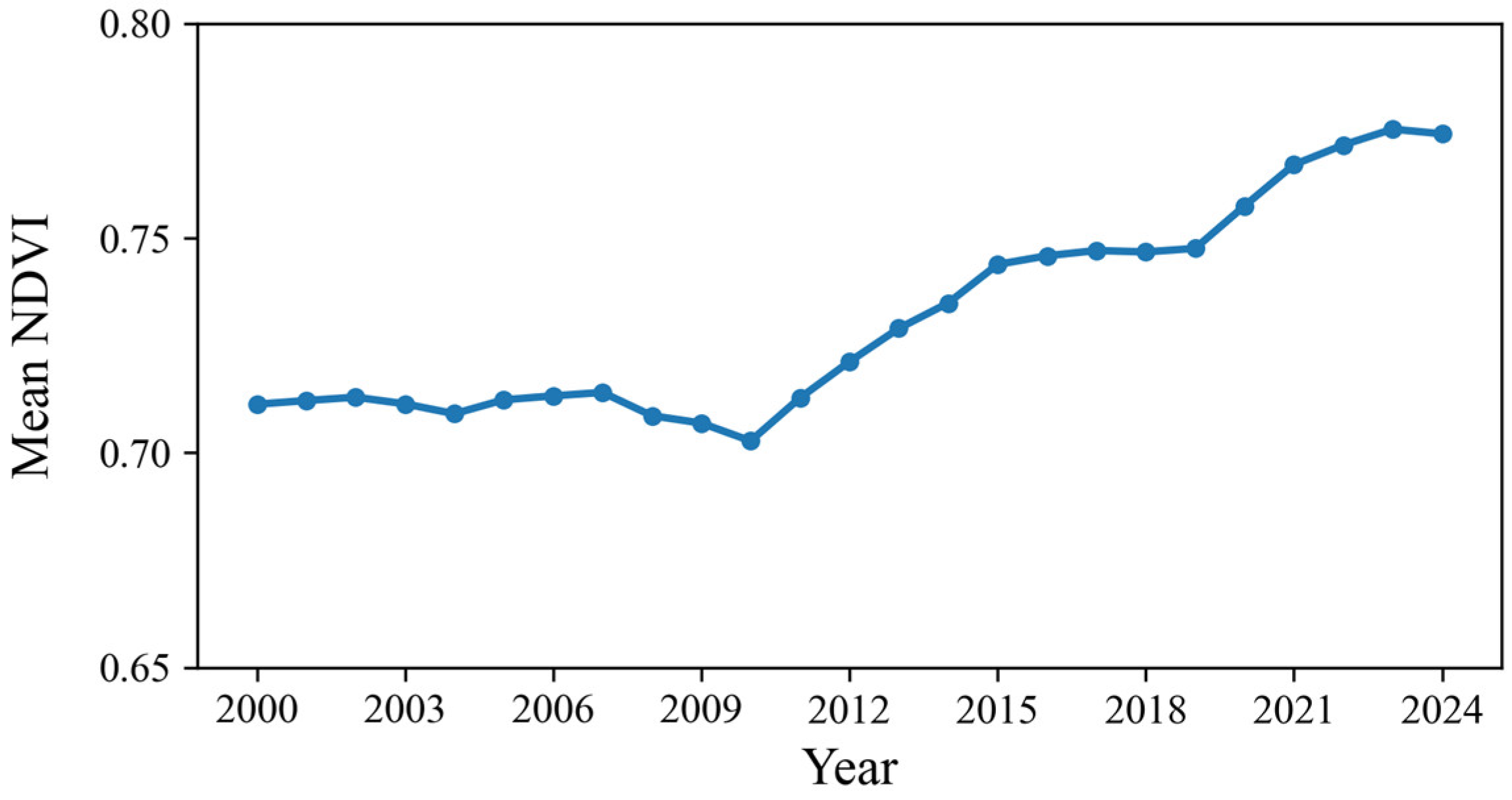
In this study area, the time series of L_M_NDVI shows an overall upward trend with interannual fluctuations from 2000 to 2024 (Figure 4). The regional average NDVI increased from 0.711 in 2000 to 0.774 in 2024 (a net increase of 0.0629, approximately +8.84%). Before the earthquake (2000–2007), NDVI was relatively stable with a slight increase. Subsequently, a significant decline occurred from 2008 to 2010, reaching the lowest value of 0.703 in 2010, reflecting vegetation degradation signals during the short-term disturbance period after the earthquake. Since 2011, NDVI has rebounded rapidly (0.713 in 2011) and entered a period of continuous greening after 2012 (0.721 in 2012 → 0.729 in 2013, with an overall increase thereafter), reaching a peak of 0.775 in 2023. Although it slightly declined in 2024 (0.774), it remained at a high level. This phased change coincides with the post-earthquake disturbance-recovery process in time, and its ecological significance can be further corroborated by combining spatial distribution and land cover shift results.

Although the curve in Figure 4 visually suggests weakening around 2007, a formal breakpoint analysis identified 2008 as the statistically significant transition year (Chow test: F = 53.58, p < 0.001). This suggests that the structural shift in the NDVI series is more robustly associated with 2008 than with 2007.

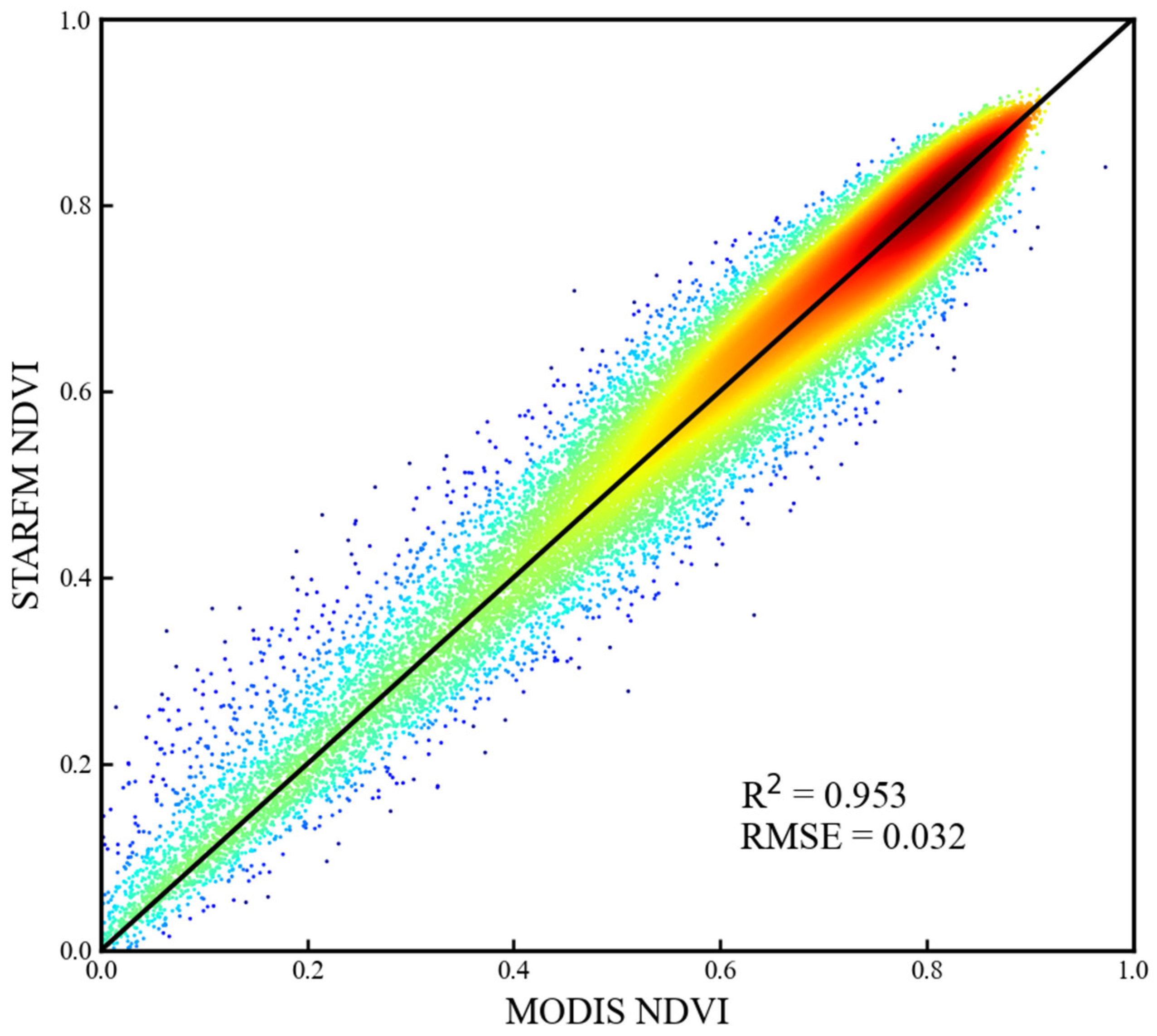
We randomly selected 100,000 discrete points and compared the resampled L_M_NDVI time series with the MODIS data from the same year, pixel-by-pixel at the same location [26]. The discrete points of the fused image and MODIS NDVI are basically distributed on the y = x plane. The correlation coefficient R² between the two sets of data reaches 0.953 and root mean square error (RMSE) of 0.032 (Figure 5). Therefore, the fused image fully captures the spectral information of MODIS NDVI during the same period and can be used as a data source for analyzing vegetation cover characteristics.

To provide both baseline comparison and independent validation, we compared MODIS-only, Landsat-only, and STARFM-derived NDVI against HLS/Sentinel-2 observations during 2018–2024 (

Table 2. Accuracy validation of different NDVI products against HLS/Sentinel-2 references.

Product	Scale	R2	RMSE	MAE
STARFM	30 m	0.732	0.080	0.061
MODIS-only	250 m	0.686	0.086	0.069
Landsat-only	250 m	0.740	0.084	0.053
STARFM	250 m	0.793	0.071	0.056

). At the 250 m scale, STARFM achieved the best agreement with the independent reference (R² = 0.793, RMSE = 0.071, MAE = 0.056), outperforming MODIS-only and Landsat-only products. At the native 30 m scale, STARFM still maintained reasonable consistency with HLS (R² = 0.732), indicating that the reconstructed series preserved spatial detail while remaining broadly reliable.

3.2. Temporal Dynamics and Forest Fraction Transitions

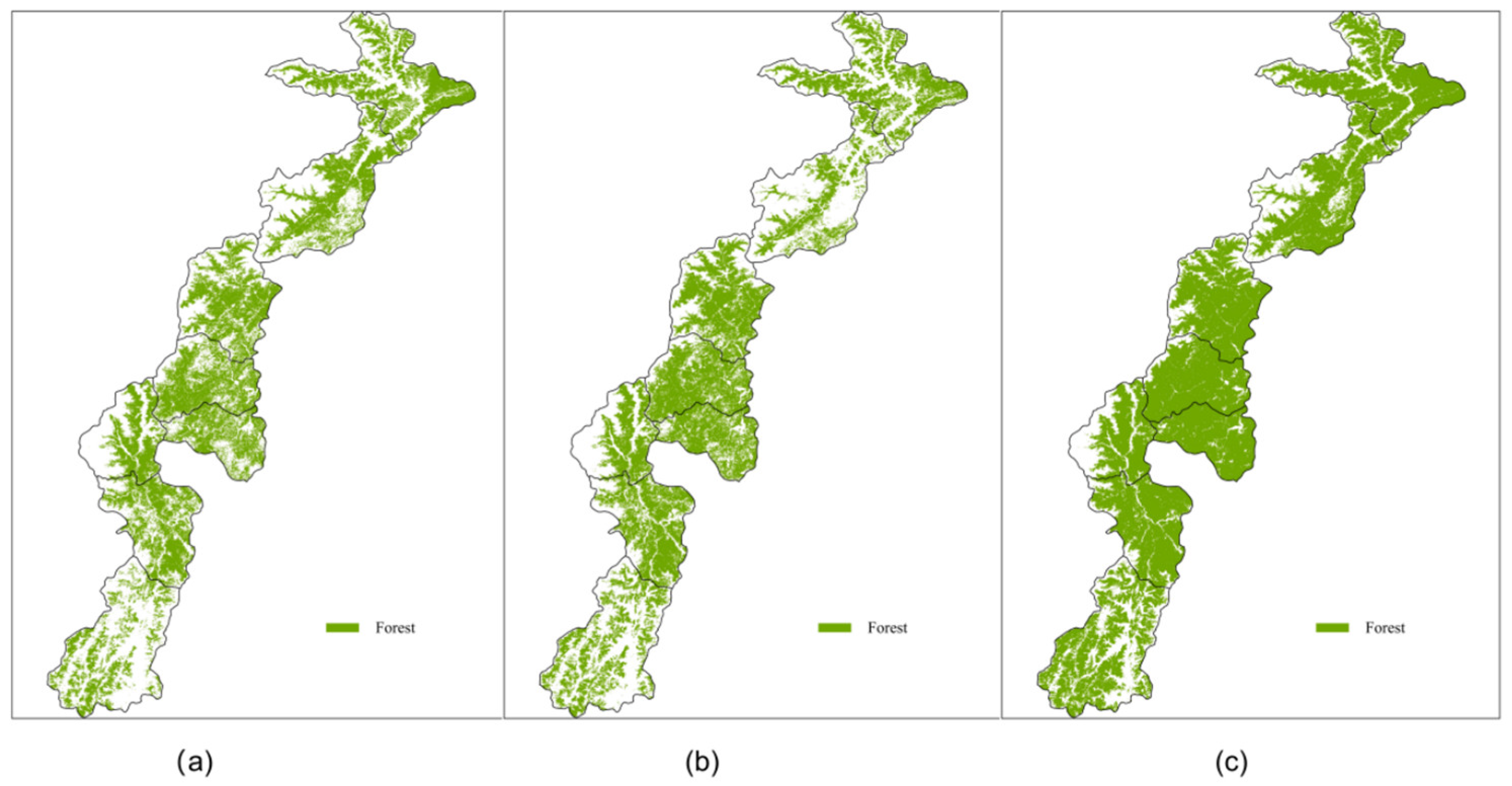
Our analysis of forest cover change reveals a substantial expansion of forest fraction in the study area from 2000 to 2024, progressively transforming the landscape from a mixed forest–non-forest pattern to a forest-dominated one (Figure 6).

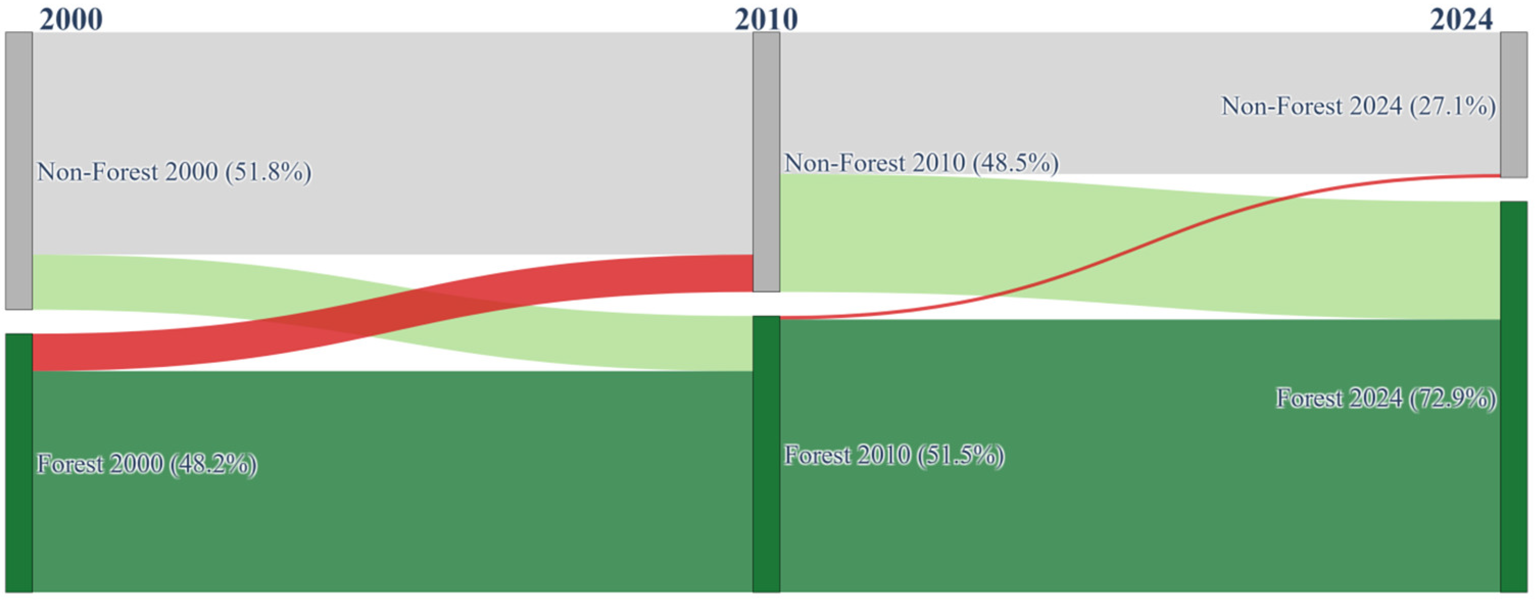
In 2000 (Figure 6a), non-forest areas accounted for 51.8% of the region, while forest cover comprised 48.2%, indicating an almost balanced landscape composition. By 2010 (Figure 6b), forest cover had increased modestly to 51.5%. In contrast, a pronounced acceleration in forest expansion occurred between 2010 and 2024 (Figure 6c), with forest fraction rising to 72.9%, representing a 21.4% increase relative to 2010. Correspondingly, non-forest areas declined sharply, occupying only 27.1% of the study area by 2024.

As summarized in

Table 3. Accuracy metrics for the forest/non-forest classification under a single split and repeated random splits (n = 5).

Validation Scheme	OA	Kappa	F1 (Forest)	F1 (Non-Forest)	Balanced Accuracy
Single split	0.863	0.724	0.870	0.855	0.862
Repeated split (n = 5)	0.852 ± 0.0037	0.704 ± 0.0075	0.854 ± 0.0063	0.851 ± 0.0033	0.852 ± 0.0037

, the forest/non-forest classification achieved good overall accuracy and remained stable across repeated random splits, suggesting that the estimated long-term forest-fraction changes were not driven by a particular sample partition. This indicates that the reported increase in forest fraction is unlikely to be an artifact of a specific train–test split and that the overall upward trend is robust across sample partitions, although some uncertainty may still remain in the exact magnitude of the change.

To visualize the dynamic changes in forest and non-forest fraction, we constructed a Sankey diagram (Figure 7). This diagram summarizes the land cover composition each year and the direction and magnitude of transitions between adjacent periods. In 2000, the landscape was nearly balanced, with non-forest (51.8%) slightly exceeding forest (48.2%). By 2010, the overall composition had changed only slightly, with forest increasing to 51.5% and non-forest decreasing to 48.5%. During 2000–2010, forest reduction and increase occurred simultaneously and at similar scales: approximately 1679 km² of forest shifted to non-forest, and approximately 2472 km² shifted to forest. Net changes in forest fraction were limited during this period, and the forest fraction structure remained generally stable.

In contrast, forest cover changes from 2010 to 2024 are quite different. The most striking feature is the robust conversion from non-forest to forest. During this period, the area of newly added forests (approximately 5290 square kilometers) far exceeded the area of forest loss (approximately 159 square kilometers), resulting in a significant expansion of forest fraction to 72.9% in 2024, while the non-forested area shrank to 27.1%. The reverse conversion (forest to non-forest) is represented by only a very thin red line.

3.3. Spatiotemporal Patterns of Vegetation Trajectories

Based on the K-means clustering algorithm, we divided the pixel-level NDVI time series from 2000 to 2024 into four categories: continuous growth, initial decline followed by increase, initial increase followed by decline, and relatively stable. The results show that the two types representing vegetation improvement (continuous growth and initial decline followed by increase) together account for 70.95% (

Table 4. Area and proportion of the four NDVI trajectory clusters derived from pixel-wise NDVI time-series clustering across the study area (2000–2024).

Cluster Type	Area (km2)	Percent
Relatively Stable	3063.57	12.72%
Persistently Increasing	9205.31	38.22%
Decrease-then-Increase	7880.37	32.73%
Increase-then-Decrease	3929.05	16.33%

). This overwhelming proportion indicates that despite the strong earthquake that disrupted the region, vegetation restoration and growth remained the dominant trend over the 24 years.

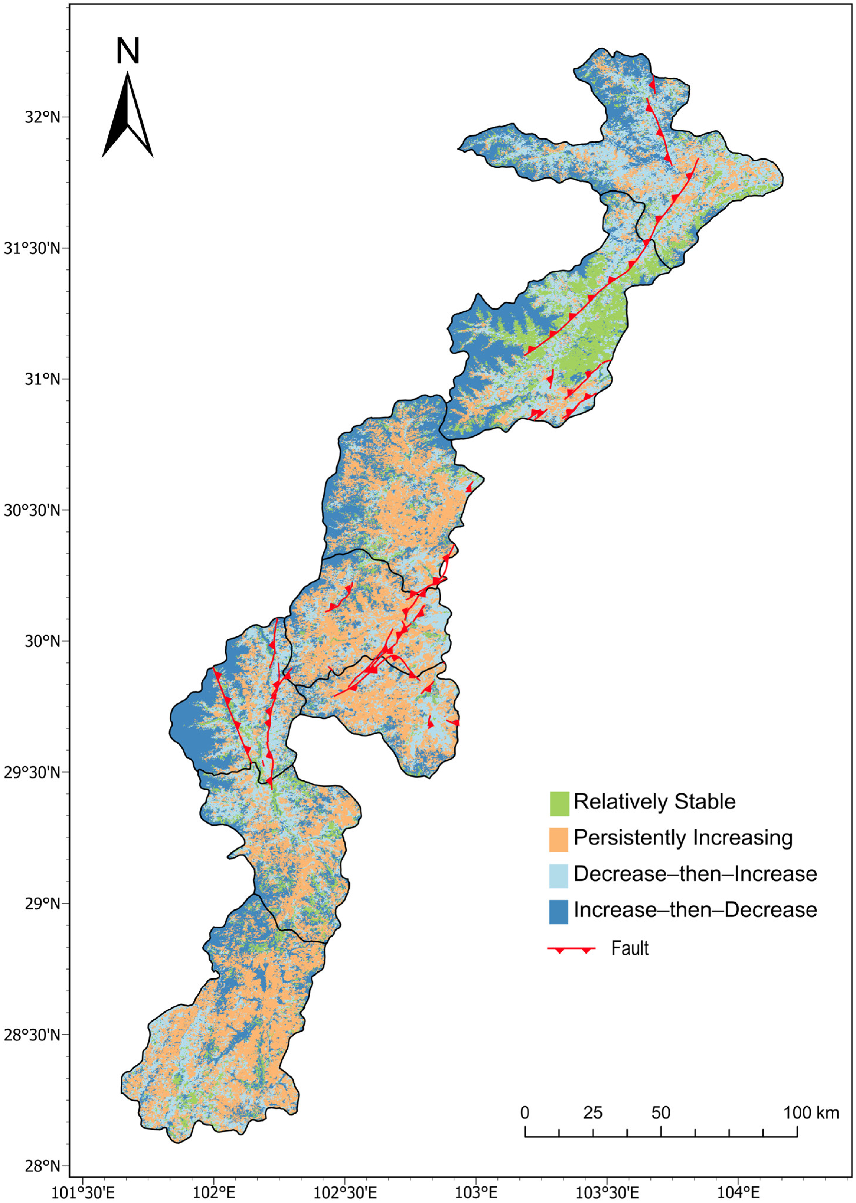
Among them, the “continuous growth” type was the most widespread, covering an area of 9205.31 km², accounting for 38.22% (Table 4). This pixel type is clustered toward the center and south of the study region, including non-severely affected areas such as Tianquan County, Yingjing County, and Shimian County (Figure 8). The NDVI shows a stable upward trend, reflecting the superior hydrothermal conditions in this type of area, as well as the effects of long-term national ecological projects such as “Natural Forest Protection” and “Returning Farmland to Forest.”

The second largest category, “decline followed by increase,” covers an area of 7880.37 km², accounting for 32.73% (Table 4), temporally consistent with post-2008 disturbance and subsequent recovery. This type of pixel is mainly distributed along the Longmenshan fault zone and its southern extension, as well as associated fault systems in the northern and central-eastern parts of the study area, including severely affected areas such as Wenchuan County and Maoxian County (Figure 8). The NDVI of this type of pixel exhibits a “V”-shaped trend: NDVI declined continuously in 2008 and then entered a fluctuating upward phase around 2010. The results suggest a disturbance–recovery pattern after 2008, through natural and artificial restoration, reflecting the resilience of the ecosystem.

Secondly, the “increase followed by decrease” type covers 3929.05 km², accounting for 16.33% (Table 4). This type of pixel initially shows an increasing trend, but the NDVI decreases later, indicating that the ecological restoration system in some areas remains vulnerable. Furthermore, the “relatively stable” type (12.72%) is mainly distributed in patches in high-altitude mountainous areas and undisturbed primary forest areas. These areas are less affected by human activities, have stable ecosystems, and their NDVI remains relatively stable.

Kruskal–Wallis tests further showed clear environmental differentiation among the four trajectory classes, with the strongest between-class differences observed for elevation (H = 7590), followed by population density (H = 4507) and slope (H = 967). The RF-based reclassification further supported the separability of the trajectory types. Across repeated runs, the classifier achieved an OA of 0.655 ± 0.005, a Macro-F1 of 0.655 ± 0.005, a balanced accuracy of 0.655 ± 0.005, and a Kappa of 0.540 ± 0.007, all clearly above the random four-class baseline. These results indicate that the identified trajectory classes were not only temporally distinct but also moderately separable in terms of their environmental backgrounds.

Moreover, the decline-followed-by-increase trajectory (Cluster 3) showed the strongest enrichment in post-event LL residual hotspots (ER = 2.31, OR = 3.06, p < 0.001), indicating that this trajectory type was spatially consistent with localized negative anomalies after 2008 rather than being a purely algorithmic artifact.

3.4. Driving Mechanisms Based on MORF and SHAP

To quantitatively reflect the correspondence between annual NDVI sequences from 2000 to 2024 and anthropogenic and natural factors, we constructed a multi-output random forest (MORF) model. Topography (elevation, slope, aspect, topographic relief), climate (annual mean temperature, annual precipitation), land-cover composition (fractions of forest, cropland, grassland, built-up areas, and water), and population density were used as input features X. A 25-dimensional vector composed of NDVI data from 2000 to 2024 was used as the supervised learning objective Y. We employed GroupKFold (5-fold) cross-validation over 10 km spatial blocks and used out-of-fold (OOF) prediction results to evaluate model performance. The model exhibited high overall goodness of fit under OOF conditions, with a micro-mean R² of 0.8754, and the R² remained consistently above 0.87 each year, indicating that the model can reconstruct the spatial distribution differences in NDVI relatively stably, offering a dependable basis for subsequent variable contribution attribution.

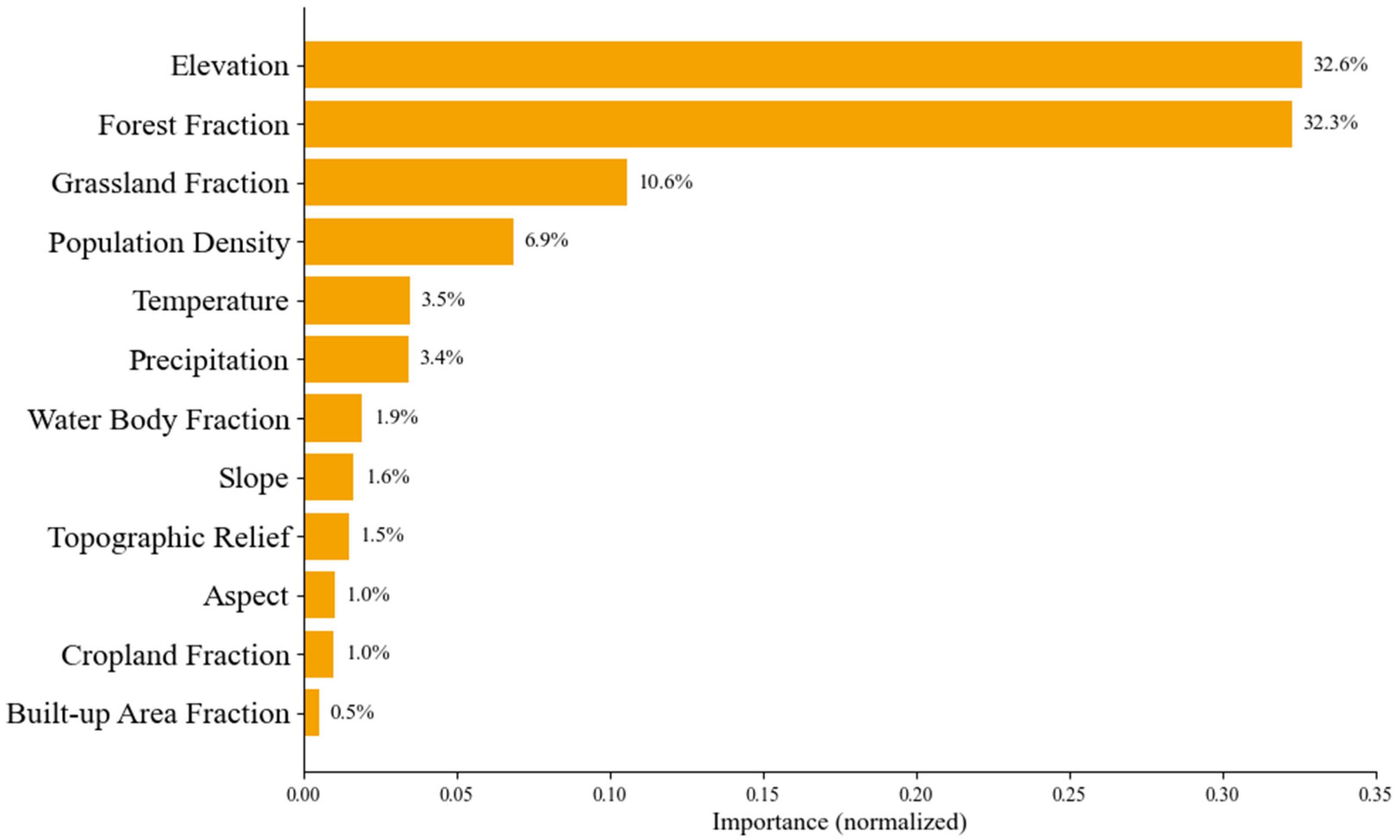
Among all variables, contributions exhibit a significant “head-concentration” characteristic (Figure 9): altitude (32.6%) and forest fraction (32.3%) are the two most important explanatory factors, accounting for approximately 65% of the total importance. Grassland cover (10.6%) ranks third, followed by population density (6.9%). Climate factors have relatively low importance, with average annual temperature and annual precipitation contributing 3.5% and 3.4%, respectively. Additionally, water cover contributes 1.9%. These top seven variables collectively explain approximately 91% of the total importance. The remaining variables (e.g., slope, aspect, topographic relief, proportion of cultivated land, proportion of construction land) contribute relatively little (less than 1.7%), thus having limited contribution to the overall explanatory power of the model.

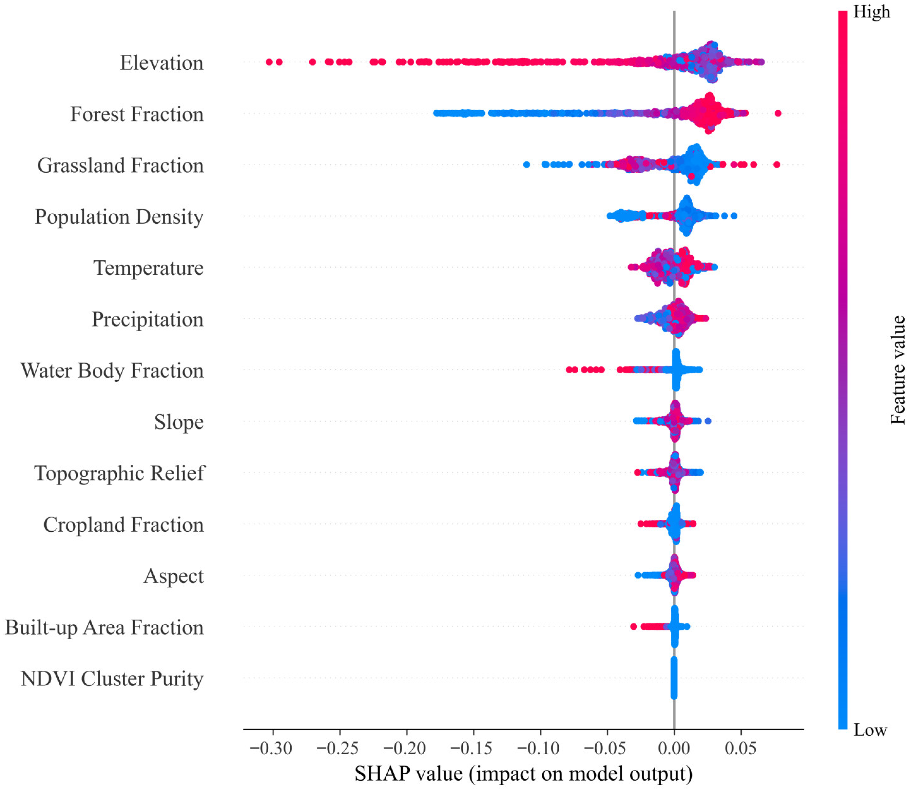
Furthermore, we calculated and summarized the mean SHAP value (mean_2000_2024) of the multi-output model from 2000 to 2024, obtaining the SHAP point cloud distribution for the entire period (Figure 10). Overall, samples with a high forest fraction mostly showed positive SHAP values; conversely, high-altitude samples mainly showed negative SHAP values with long negative tails, indicating that high-altitude areas are unfavorable for vegetation growth, and this effect varied significantly across different pixels. Grassland and water body ratios also showed negative contributions under high SHAP conditions, revealing a close correlation between land cover differences and NDVI spatial differentiation. In contrast, the SHAP distribution of annual mean temperature and annual precipitation was more concentrated near zero, reflecting their smaller contribution to NDVI spatial variation. The impact of population density was generally small but concentrated in local areas, indicating that the influence of human activities on NDVI spatial patterns has strong local characteristics. The results show that the long-term spatial characteristics of NDVI in the study area are mainly related to topography and vegetation/land cover, while the contributions of climate factors and other variables are relatively small (Figure 9).

We further compared the multi-output random forest (MORF) with a linear baseline and a single-output random forest (SORF). The linear model showed much lower explanatory power (R² = 0.3518), whereas SORF and MORF achieved similarly high performance (R² = 0.8798 and 0.875, respectively). Given this comparable accuracy, MORF was retained because it jointly models multi-year NDVI responses within a unified framework, which is more consistent with the objective of explaining long-term vegetation trajectories.

3.5. Interpretation of Spatial Residual Diagnostics

Spatial diagnostics of the MORF out-of-fold residuals showed significant positive spatial autocorrelation in all representative years requested by the reviewer (

Table 5. Spatial autocorrelation diagnostics for MORF residuals.

Year/Period	Moran’s I	Permutation p-Value	Significant LISA Pixels (%)	Dominant Local Patterns
2007	0.358	<0.001	18.45	HH and LL dominate; HL/LH are rare
2008	0.334	<0.001	17.57
2010	0.343	<0.001	19.33
2012	0.348	<0.001	19.16
2024	0.315	<0.001	17.29

). The proportion of significant LISA pixels ranged from 17.57% to 19.33% in the years currently summarized, and local clustering was dominated by HH and LL classes, whereas HL and LH patterns were relatively rare.

A pre-/post-2008 comparison further indicated a modest increase in residual clustering after 2008, with Moran’s I increasing from 0.34 to 0.36 and the proportion of significant LISA pixels increasing from 17.87% to 19.33% (

Table 6. Comparison of model residuals before and after the 2008 earthquake.

Period	Moran’s I	Permutation p-Value	Significant LISA Pixels (%)	HH (%)	LL (%)	Mean Absolute Residual	RMSE
Pre-2008 (2005–2007)	0.34	<0.001	17.87	8.12	8.55	0.033	0.048
Post-2008 (2009–2011)	0.36	<0.001	19.33	10.28	7.85	0.032	0.046

). In contrast, the mean absolute residual and RMSE remained similar or slightly decreased, suggesting that the post-2008 difference was expressed more in spatial organization than in overall residual magnitude.

4. Discussion

4.1. Methodological Implications: From Gap-Filling to Reliable Ecological Inference

A key contribution of this study is the reconstruction of a continuous 30 m NDVI record from 2000 to 2024 in cloudy and topographically complex mountainous areas, thereby enabling the differentiation of long-term vegetation restoration, post-disturbance stagnation, and spatially heterogeneous trajectories within a single analytical framework.

Conducting 25 years of vegetation dynamic monitoring in the topographically complex western Sichuan mountains presented a significant challenge: ensuring the continuity and consistency of the observational data. This was particularly evident when constructing long-term series spanning two generations of sensors. The Landsat 5 TM’s extended service life and eventual retirement (2011), coupled with the Landsat 8 OLI’s non-operational status before 2013 and the availability of only Landsat 7 ETM+ data (though the airborne scan line corrector malfunctioned, resulting in approximately 22% spatial banding gaps [27]), meant that damaged images or simple interpolation could easily introduce spurious abrupt changes into the time-series curves [28], severely interfering with the assessment of the critical “stagnation-recovery” transition period in post-earthquake vegetation.

Our STARFM algorithm, fusing Landsat and MODIS data, not only visually restores image integrity but also constructs a continuous and reliable NDVI time series, providing reliable data for subsequent analysis. Compared to 250 m MODIS products, which often smooth out local fragmented restoration patches due to their large pixel size [7], the fused 30 m data effectively preserves spatial heterogeneity. The high agreement with MODIS (R² = 0.953) mainly supports the temporal coherence of the reconstructed series, whereas the additional comparison against HLS/Sentinel-2 during 2018–2024 provides more independent support that STARFM outperforms the MODIS-only and Landsat-only baselines at 250 m while still maintaining reasonable consistency at the native 30 m scale.

To investigate the complex driving mechanisms of forest cover change, we employ a Multi-Output Random Forest (MORF) model for attributing driving forces. Traditional regression analysis often assumes that annual NDVI is an independent observation, thus severing the inherent temporal correlations within the ecosystem. Our MORF model, however, does not treat annual NDVI as isolated observations but treats the time series curves from 2000 to 2024 as a whole. This approach not only considers the immediate impact of environmental factors on vegetation but also better reflects the temporal dependence of vegetation growth—that is, the vegetation state in a given year is not randomly generated but is partly conditioned by its historical growth base [14] (such as the biomass accumulation of the previous year).

This interpretation is also supported by the baseline comparison: the linear model showed much lower explanatory power (R² = 0.3518), whereas SORF and MORF achieved similarly high performance (R² = 0.8798 and 0.875, respectively), indicating that the main gain comes from accommodating nonlinear relationships rather than from an explicit year-by-year linear specification. In addition, the out-of-fold residual diagnostics revealed significant but moderate spatial autocorrelation, and the pre-/post-2008 comparison showed a slight increase in residual clustering after the earthquake without a corresponding increase in residual magnitude, suggesting that the model captured the dominant large-scale signal while still leaving some localized spatial structure unexplained.

4.2. Topographic and Biotic Constraints Govern Vegetation Heterogeneity

Our multi-output random forest model identified elevation (32.6%) as the most influential predictor, although this result should be interpreted cautiously. High-altitude samples (red dots) cluster in the negative SHAP range (Figure 10), reflecting the significant inhibitory effect of high altitude on forests. This is consistent with the vertical zonation theory, which posits that the scarcity of water and heat resources in high-altitude areas strictly limits the upper limit of vegetation survival [29]. In the mountainous western Sichuan Basin, elevation is likely to play an important role in shaping treeline position and ecological niche differentiation [30]. The apparent contribution of elevation was substantially higher than that of long-term mean temperature (3.5%) and precipitation (3.4%). However, this does not necessarily mean that topography alone dominates vegetation dynamics; rather, elevation may partly act as an integrated proxy for topo-hydroclimatic variation and biogeographic differentiation within the study area [31]. This interpretation is also supported by the moderate negative correlations of elevation with temperature (r = −0.5976) and precipitation (r = −0.4878), suggesting that the elevation effect likely absorbs part of the broader environmental gradient rather than representing a purely geomorphological constraint. In addition, because the forest map used here is binary rather than type-specific, part of the apparent elevation effect may also reflect altitudinal differentiation in forest composition, with broadleaf forests more common at lower elevations, mixed forests in mid-elevation zones, and coniferous forests more frequent at higher elevations. Differences in species composition, canopy structure, and phenological behavior among these forest types may influence NDVI magnitude and seasonal dynamics, thereby contributing to the observed importance of elevation.

The high contributions of initial forest proportion (32.3%) and grassland proportion (10.6%) reflect the crucial role of “biological heritage” in post-disaster forest system restoration [32]. The SHAP summary plot analysis reveals that a higher initial forest cover consistently contributes positively to the model output. This strongly supports the nucleation theory of succession, indicating that existing vegetation patches act as “bioanchors” [33]. These patches may accelerate the recovery of neighboring areas through positive feedback loops, such as improvements in microclimates [34], thereby accelerating ecosystem recovery.

Notably, the impact of population density (6.9%) is greater than that of natural climate, a finding often masked in lower-resolution studies [35]. The SHAP summary plot (Figure 10) visually shows that samples with high population density (red dots) are concentrated in the negative SHAP range, indicating their inhibition of vegetation growth. This result reveals the exacerbated “human-land conflict” due to topographic constraints. In our study area, high population density is mainly concentrated in relatively flat river valleys. These areas should be the most favorable vegetation growth zones in terms of hydrothermal conditions but are now occupied by urbanization and farmland [36]. The negative feedback of SHAP values confirms that, within limited space, high-intensity human disturbance has a significant negative impact on vegetation growth.

4.3. The Imprint of the Wenchuan Earthquake on Forest Recovery Dynamics

The reconstructed long-term continuous NDVI exhibits a clear “decline-stagnation-recovery” trajectory. The average NDVI in the study area remained stable between 2000 and 2008, declined after 2008, but accelerated in 2012 (Figure 4). The time inflection point of the NDVI time series in this study is highly consistent with the findings of Yang and Qi [37]. They found that the most significant decline in vegetation loss (ED_NDVI) occurred in 2013 and 2014, a time lag indicating that the severely damaged ecosystem actually experienced a stagnation period lasting several years before entering a rapid recovery phase.

This temporary stagnation may reflect an earthquake-related disturbance legacy. Unlike fire or deforestation, the Wenchuan earthquake was associated with widespread “vegetation-soil system co-degradation.” As Cui et al. [21] pointed out, the widespread presence of loose material and degraded soil structure inhibited rapid vegetation recovery in the early stages. The ecosystem needs a “stagnation period” for slope compaction and soil crusting, which is beneficial for vegetation growth.

Following 2012, forests recovered rapidly, largely thanks to human intervention. The Chinese government designated a five-year post-disaster reconstruction period (2008–2013) [38], and the surge in our NDVI sequence coincides temporally with the implementation of these large-scale ecological projects, such as afforestation.

This “V”-shaped trajectory of NDVI within the study area reflects a pattern of “decreasing then increasing” (accounting for 32.73% of the total area). This type of pixel is concentrated in high-intensity disaster areas such as Wenchuan and Maoxian. This finding refines the “fluctuating” recovery pattern identified by Yang and Qi [37], which is mainly distributed in the northeastern part of the epicenter (such as Maoxian). Limited by the study period ending in 2014, these areas at that time exhibited a lack of consistent recovery trends. Our NDVI time series from 2000 to 2024 reflects that the “fluctuation” is actually a “stagnant” phase within the “decreasing then increasing” trajectory.

Additional support for this interpretation comes from the residual-based spatial diagnostics. The OOF residual analyses using Global Moran’s I, Local Moran’s I/LISA, and pre-/post-event residual contrasts showed that MORF residuals still retained significant spatial autocorrelation, with slightly stronger local clustering after the earthquake. When the K-means trajectories were further overlaid with post-event LISA hotspots, the decline-followed-by-increase group exhibited the strongest enrichment in post-event LL residual hotspots (ER = 2.31, OR = 3.06, p < 0.001). This spatial correspondence suggests that the trajectory is consistent with localized negative anomalies after 2008 and therefore provides additional evidence that it reflects a disturbance–recovery process rather than a purely statistical artifact.

4.4. Uncertainties and Future Perspectives

While this study revealed the dynamic evolution of forest restoration in the western Sichuan forest region, certain uncertainties remain due to limitations in remote sensing inversion technology and the complex mountainous environment. To provide a more formal assessment of the remaining uncertainty in the present workflow, we distinguish three major sources of uncertainty in this study: uncertainty in NDVI reconstruction, uncertainty in forest/non-forest classification, and uncertainty in driver attribution/modeling. Their current controls, remaining limitations, and possible propagation across workflow stages are summarized in

Table 7. Summary of key uncertainty sources, their remaining limitations, and their potential propagation within the study workflow.

Uncertainty Source	Current Control	Remaining Limitation	Potential Propagation to Downstream Analysis
NDVI Reconstruction	MODIS consistency check; HLS/Sentinel-2 baseline comparison	Early-period independent validation is limited; terrain fragmentation may affect local spatial accuracy	May influence local NDVI magnitude and boundary delineation, thereby affecting subsequent classification in fragmented or transitional pixels
Forest/non-forest classification	Accuracy metrics under a single split; a repeated random split robustness test	Boundary pixels and mixed transitional areas may still be misclassified	May affect the exact magnitude and local spatial pattern of forest-cover change and transition-area estimates used for ecological interpretation
Driver attribution/modeling	Linear/SORF/MORF baseline comparison; spatial block CV; OOF Moran’s I/LISA diagnostics	Residual local spatial structure remains; no explicit earthquake-distance variables are included	Supports the main driver-ranking pattern, but local attribution should remain cautious and may partly reflect uncertainty propagated from upstream reconstruction and classification stages

. Importantly, these uncertainties are not fully independent: uncertainty introduced during NDVI reconstruction may propagate into the annual forest/non-forest classification, which may in turn affect estimates of forest-cover change and the interpretation of downstream driver attribution.

Firstly, regarding the accuracy verification scheme, the extremely high consistency (R² = 0.953) between fused NDVI and MODIS NDVI primarily confirms the ability of the fused sequence to capture regional macro-phenological trends. However, this verification process inherently depends on MODIS data, essentially focusing more on assessing the STARFM’s preservation of temporal frequency, while its verification of sub-pixel spatial details at the Landsat scale—especially the subtle vegetation fluctuations in areas of topographic fragmentation—is still insufficient. Considering the long-term cloud and fog obscuring the high-altitude canyon areas of western Sichuan, obtaining high-quality original Landsat images that perfectly match the fusion time and have no stripe loss as independent “ground truth” is extremely challenging, which to some extent limits the accuracy of evaluating disturbance events at extremely small spatial scales. Future work should therefore prioritize validation against more independent high-resolution references, such as Sentinel-2/HLS products or field-based observations, to better assess Landsat-scale spatial accuracy in heterogeneous mountain terrain. Such reconstruction uncertainty may affect local NDVI magnitude, blur boundary delineation, and reduce the separability of forest and non-forest signals, particularly in fragmented, transitional, or topographically complex landscapes. Consequently, it may propagate into the subsequent forest/non-forest classification by increasing uncertainty in boundary and mixed pixels, which may in turn affect local estimates of forest-cover change and their ecological interpretation.

In addition, the vast elevation range (598–7439 m) and dramatic topographic relief in the study area continuously interfere with the reconstruction of surface reflectance. Although this study adopted a “calculate the index first, then fuse” strategy to reduce error propagation, in high-altitude shady slopes, strong topographic shading and differences in atmospheric path radiation can still cause bias in STARFM’s search for similar pixels for weight allocation. This topographic effect not only affects the absolute value of NDVI inversion but may also interfere with the accurate definition of the “lag period” length of forest restoration. Future research should attempt to introduce more refined topographic correction models or use independent observation sources with higher revisit frequencies, such as Sentinel-2, for spatial cross-validation to further eliminate the noise interference of topographic effects on time-series curves.

Secondly, uncertainty also remains in the annual forest/non-forest classification. Although the classification achieved good overall accuracy and remained stable across repeated random splits, classification errors may still occur for boundary pixels, mixed land-cover mosaics, and transitional environments under the binary forest/non-forest framework. These errors are unlikely to overturn the overall increasing trend in forest fraction, but they may affect the exact magnitude, local spatial pattern, and transition-area estimates. Because the classification outputs are subsequently used to summarize forest-cover change and support ecological interpretation, this stage represents an important pathway through which upstream reconstruction uncertainty can be translated into downstream change estimates.

Taken together, uncertainty in this workflow should be understood as cumulative rather than fully stage-specific. Errors introduced during NDVI reconstruction can affect both the magnitude of annual NDVI values and the separability of forest and non-forest signals, especially in fragmented, transitional, or topographically complex areas. This uncertainty may then propagate into the annual forest/non-forest classification, influencing boundary assignment, transition-area estimates, and the spatial delineation of local change hotspots. In turn, these upstream uncertainties constrain the confidence with which temporal trajectory patterns and local ecological changes can be interpreted. Therefore, uncertainty associated with downstream analysis is not entirely generated at the final modeling stage but is partly inherited from the earlier reconstruction and classification stages.

Thirdly, in terms of the depth of driving force attribution, the MORF model mainly selected relatively steady-state factors such as topography, multi-year average climate, and population density. While these factors effectively explain spatial zonal differences (such as the dominant role of elevation and initial forest percentage), the restoration of forest ecosystems is a nonlinear process driven by both natural succession and dynamic policy disturbances. Earthquake-induced “vegetation-soil system co-degradation” involves deep underground ecological succession, while the instantaneous impact of extreme climate events (such as anomalous droughts) on the recovery trajectory has not been fully characterized in the current attribution system based on static factors. Future research needs to integrate higher-frequency dynamic environmental monitoring indicators and combine them with field-measured soil physicochemical properties to explore in depth the response mechanisms and recovery bottlenecks of mountain ecosystems under multiple disturbances. In addition, although the residual-based spatial diagnostics helped reveal remaining spatial structure, explicit distance-to-fault or distance-to-epicenter variables were not included in the attribution framework, so the earthquake interpretation should still be viewed as supported but not fully causal. Accordingly, uncertainty at the attribution stage should not be interpreted as entirely model-specific, because part of it may reflect uncertainty inherited from the earlier reconstruction and classification stages.

5. Conclusions

In this study, we reconstructed a long-term (2000–2024), high-resolution (30 m) vegetation record for the western Sichuan Basin using the STARFM algorithm and quantified the driving mechanisms of forest recovery using a Multi-output Random Forest (MORF) model. The main conclusions are summarized as follows:

1.

High-fidelity data reconstruction: The STARFM algorithm effectively mitigated cloud contamination and sensor defects (e.g., Landsat 7 SLC-off), generating a robust NDVI time series that agrees well with valid observations (${\mathrm{R}}^2=0.953$). This fused dataset captured fine-scale spatial details of forest fragmentation that were obscured in coarse-resolution products.

2.

“Stagnation-then-Recovery” trajectory: The region exhibited a non-linear recovery pattern characterized by a post-seismic stagnation phase (2000–2010) followed by accelerated greening. Forest fraction increased substantially from 51.5% in 2010 to 72.9% in 2024, driven primarily by the unidirectional conversion of non-forest areas to forests in earthquake-impacted zones.

3.

Topography-dominated driving mechanisms: The spatial heterogeneity of vegetation recovery was more strongly governed by topographic and biotic constraints than by climatic variability. Elevation and initial forest fraction were identified as the dominant drivers, collectively accounting for over 60% of feature importance, suggesting that vertical zonation and biotic legacies determine the boundaries of post-disaster ecosystem restoration.

Our results indicate that post-seismic greening is not spatially uniform but is bounded by strong elevational controls and biotic legacies (initial forest fraction). This suggests that restoration planning should explicitly incorporate terrain-constrained suitability, avoiding uniform interventions across heterogeneous mountain landscapes. Priority should be given to protecting remnant forest patches and high-recovery “nucleation” areas, as they likely function as key seed sources and regeneration hubs. Assisted restoration (e.g., enrichment planting) can then be strategically deployed in elevation bands and slope contexts where the NDVI trajectory demonstrates stable recovery, while persistently constrained zones may require complementary measures such as erosion control and landslide-risk mitigation. Finally, continuous high-resolution monitoring is recommended to evaluate the effectiveness of these targeted actions and to adjust strategies as recovery progresses.

References

1. Brockerhoff, E.G.; Barbaro, L.; Castagneyrol, B.; Forrester, D.I.; Gardiner, B.; González-Olabarria, J.R.; Lyver, P.O.; Meurisse, N.; Oxbrough, A.; Taki, H.; et al. Forest Biodiversity, Ecosystem Functioning and the Provision of Ecosystem Services. Biodivers. Conserv. 2017, 26, 3005–3035. [Google Scholar] [CrossRef] [Scilit]
2. Hua, F.; Bruijnzeel, L.A.; Meli, P.; Martin, P.A.; Zhang, J.; Nakagawa, S.; Miao, X.; Wang, W.; McEvoy, C.; Peña-Arancibia, J.L.; et al. The Biodiversity and Ecosystem Service Contributions and Trade-Offs of Forest Restoration Approaches. Science 2022, 376, 839–844. [Google Scholar] [CrossRef] [Scilit] [PubMed]
3. Folke, C.; Carpenter, S.; Walker, B.; Scheffer, M.; Elmqvist, T.; Gunderson, L.; Holling, C.S. Regime Shifts, Resilience, and Biodiversity in Ecosystem Management. Annu. Rev. Ecol. Evol. Syst. 2004, 35, 557–581. [Google Scholar] [CrossRef] [Scilit]
4. Zhu, Z.; Woodcock, C.E. Automated Cloud, Cloud Shadow, and Snow Detection in Multitemporal Landsat Data: An Algorithm Designed Specifically for Monitoring Land Cover Change. Remote Sens. Environ. 2014, 152, 217–234. [Google Scholar] [CrossRef] [Scilit]
5. Rial, J.A.; Pielke, R.A.; Beniston, M.; Claussen, M.; Canadell, J.; Cox, P.; Held, H.; De Noblet-Ducoudré, N.; Prinn, R.; Reynolds, J.F.; et al. Nonlinearities, Feedbacks and Critical Thresholds within the Earth’s Climate System. Clim. Change 2004, 65, 11–38. [Google Scholar] [CrossRef] [Scilit]
6. Chen, J.; Zhu, X.; Vogelmann, J.E.; Gao, F.; Jin, S. A Simple and Effective Method for Filling Gaps in Landsat ETM+ SLC-off Images. Remote Sens. Environ. 2011, 115, 1053–1064. [Google Scholar] [CrossRef] [Scilit]
7. Garrigues, S.; Allard, D.; Baret, F.; Weiss, M. Quantifying Spatial Heterogeneity at the Landscape Scale Using Variogram Models. Remote Sens. Environ. 2006, 103, 81–96. [Google Scholar] [CrossRef] [Scilit]
8. Gao, F.; Masek, J.; Schwaller, M.; Hall, F. On the Blending of the Landsat and MODIS Surface Reflectance: Predicting Daily Landsat Surface Reflectance. IEEE Trans. Geosci. Remote Sens. 2006, 44, 2207–2218. [Google Scholar] [CrossRef] [Scilit]
9. Zhu, X.; Chen, J.; Gao, F.; Chen, X.; Masek, J.G. An Enhanced Spatial and Temporal Adaptive Reflectance Fusion Model for Complex Heterogeneous Regions. Remote Sens. Environ. 2010, 114, 2610–2623. [Google Scholar] [CrossRef] [Scilit]
10. Liu, M.; Yang, W.; Zhu, X.; Chen, J.; Chen, X.; Yang, L.; Helmer, E.H. An Improved Flexible Spatiotemporal DAta Fusion (IFSDAF) Method for Producing High Spatiotemporal Resolution Normalized Difference Vegetation Index Time Series. Remote Sens. Environ. 2019, 227, 74–89. [Google Scholar] [CrossRef] [Scilit]
11. Tian, F.; Wang, Y.; Fensholt, R.; Wang, K.; Zhang, L.; Huang, Y. Mapping and Evaluation of NDVI Trends from Synthetic Time Series Obtained by Blending Landsat and MODIS Data around a Coalfield on the Loess Plateau. Remote Sens. 2013, 5, 4255–4279. [Google Scholar] [CrossRef] [Scilit]
12. Rao, Y.; Zhu, X.; Chen, J.; Wang, J. An Improved Method for Producing High Spatial-Resolution NDVI Time Series Datasets with Multi-Temporal MODIS NDVI Data and Landsat TM/ETM+ Images. Remote Sens. 2015, 7, 7865–7891. [Google Scholar] [CrossRef] [Scilit]
13. Fan, M.; Ma, D.; Huang, X.; An, R. Adaptability Evaluation of the Spatiotemporal Fusion Model of Sentinel-2 and MODIS Data in a Typical Area of the Three-River Headwater Region. Sustainability 2023, 15, 8697. [Google Scholar] [CrossRef] [Scilit]
14. Ogle, K.; Barber, J.J.; Barron-Gafford, G.A.; Bentley, L.P.; Young, J.M.; Huxman, T.E.; Loik, M.E.; Tissue, D.T. Quantifying Ecological Memory in Plant and Ecosystem Processes. Ecol. Lett. 2015, 18, 221–235. [Google Scholar] [CrossRef] [Scilit]
15. Kharrazi, A.; Kraines, S.; Hoang, L.; Yarime, M. Advancing Quantification Methods of Sustainability: A Critical Examination of Emergy, Exergy, Ecological Footprint, and Ecological Information-Based Approaches. Ecol. Indic. 2014, 37, 81–89. [Google Scholar] [CrossRef] [Scilit]
16. Verbesselt, J.; Hyndman, R.; Newnham, G.; Culvenor, D. Detecting Trend and Seasonal Changes in Satellite Image Time Series. Remote Sens. Environ. 2010, 114, 106–115. [Google Scholar] [CrossRef] [Scilit]
17. Dormann, C.F.; Elith, J.; Bacher, S.; Buchmann, C.; Carl, G.; Carré, G.; Marquéz, J.R.G.; Gruber, B.; Lafourcade, B.; Leitão, P.J.; et al. Collinearity: A Review of Methods to Deal with It and a Simulation Study Evaluating Their Performance. Ecography 2013, 36, 27–46. [Google Scholar] [CrossRef] [Scilit]
18. Ben Taieb, S.; Bontempi, G.; Atiya, A.F.; Sorjamaa, A. A Review and Comparison of Strategies for Multi-Step Ahead Time Series Forecasting Based on the NN5 Forecasting Competition. Expert Syst. Appl. 2012, 39, 7067–7083. [Google Scholar] [CrossRef] [Scilit]
19. Cha, Y.; Shin, J.; Go, B.; Lee, D.-S.; Kim, Y.; Kim, T.; Park, Y.-S. An Interpretable Machine Learning Method for Supporting Ecosystem Management: Application to Species Distribution Models of Freshwater Macroinvertebrates. J. Environ. Manag. 2021, 291, 112719. [Google Scholar] [CrossRef] [Scilit]
20. Sun, H.; Zhang, J.; Deng, T.; Boufford, D.E. Origins and Evolution of Plant Diversity in the Hengduan Mountains, China. Plant Divers. 2017, 39, 161–166. [Google Scholar] [CrossRef] [Scilit]
21. Cui, P.; Lin, Y.; Chen, C. Destruction of Vegetation Due to Geo-Hazards and Its Environmental Impacts in the Wenchuan Earthquake Areas. Ecol. Eng. 2012, 44, 61–69. [Google Scholar] [CrossRef] [Scilit]
22. Viña, A.; Chen, X.; McConnell, W.J.; Liu, W.; Xu, W.; Ouyang, Z.; Zhang, H.; Liu, J. Effects of Natural Disasters on Conservation Policies: The Case of the 2008 Wenchuan Earthquake, China. AMBIO 2011, 40, 274–284. [Google Scholar] [CrossRef] [Scilit] [PubMed]
23. Li, X.; Xu, J.; Jia, Y.; Liu, S.; Jiang, Y.; Yuan, Z.; Du, H.; Han, R.; Ye, Y. Spatio-Temporal Dynamics of Vegetation over Cloudy Areas in Southwest China Retrieved from Four NDVI Products. Ecol. Inform. 2024, 81, 102630. [Google Scholar] [CrossRef] [Scilit]
24. Jarihani, A.; McVicar, T.; Van Niel, T.; Emelyanova, I.; Callow, J.; Johansen, K. Blending Landsat and MODIS Data to Generate Multispectral Indices: A Comparison of “Index-Then-Blend” and “Blend-Then-Index” Approaches. Remote Sens. 2014, 6, 9213–9238. [Google Scholar] [CrossRef] [Scilit]
25. Zhang, B.; Zhang, L.; Xie, D.; Yin, X.; Liu, C.; Liu, G. Application of Synthetic NDVI Time Series Blended from Landsat and MODIS Data for Grassland Biomass Estimation. Remote Sens. 2015, 8, 10. [Google Scholar] [CrossRef] [Scilit]
26. Fan, X.; Gao, P.; Tian, B.; Wu, C.; Mu, X. Spatio-Temporal Patterns of NDVI and Its Influencing Factors Based on the ESTARFM in the Loess Plateau of China. Remote Sens. 2023, 15, 2553. [Google Scholar] [CrossRef] [Scilit]
27. Storey, J.; Scaramuzza, P.; Schmidt, G.; Barsi, J. Landsat 7 scan line corrector-off gap-filled product development. In Global Priorities in Land Remote Sensing; ASPRS: Baton Rouge, LA, USA, 2005. [Google Scholar]
28. Hird, J.N.; McDermid, G.J. Noise Reduction of NDVI Time Series: An Empirical Comparison of Selected Techniques. Remote Sens. Environ. 2009, 113, 248–258. [Google Scholar] [CrossRef] [Scilit]
29. Chang, D.H.S. The Vegetation Zonation of the Tibetan Plateau. Mt. Res. Dev. 1981, 1, 29. [Google Scholar] [CrossRef] [Scilit]
30. Yu, H.; Miao, S.; Xie, G.; Guo, X.; Chen, Z.; Favre, A. Contrasting Floristic Diversity of the Hengduan Mountains, the Himalayas and the Qinghai-Tibet Plateau Sensu Stricto in China. Front. Ecol. Evol. 2020, 8, 136. [Google Scholar] [CrossRef] [Scilit]
31. Körner, C. Climatic Treelines: Conventions, Global Patterns, Causes (Klimatische Baumgrenzen: Konventionen, Globale Muster, Ursachen). Erdkunde 2007, 61, 316–324. [Google Scholar] [CrossRef] [Scilit]
32. Joly, C.A.; Metzger, J.P.; Tabarelli, M. Experiences from the Brazilian Atlantic Forest: Ecological findings and conservation initiatives. New Phytol. 2014, 204, 459–473. [Google Scholar] [CrossRef] [Scilit] [PubMed]
33. Morán-López, T.; Rodríguez-Pérez, J.; Donoso, I.; Martínez, D.; Morales, J.M.; García, D. Forest Recovery through Applied Nucleation: Effects of Tree Islet Size and Disperser Mobility on Tree Recruitment in a Temperate Landscape. For. Ecol. Manag. 2023, 550, 121508. [Google Scholar] [CrossRef] [Scilit]
34. Zellweger, F.; De Frenne, P.; Lenoir, J.; Vangansbeke, P.; Verheyen, K.; Bernhardt-Römermann, M.; Baeten, L.; Hédl, R.; Berki, I.; Brunet, J.; et al. Forest Microclimate Dynamics Drive Plant Responses to Warming. Science 2020, 368, 772–775. [Google Scholar] [CrossRef] [Scilit] [PubMed]
35. Li, W.; Li, X.; Tan, M.; Wang, Y. Influences of Population Pressure Change on Vegetation Greenness in China’s Mountainous Areas. Ecol. Evol. 2017, 7, 9041–9053. [Google Scholar] [CrossRef] [Scilit]
36. Hou, L.; Liu, T.; Wang, J.; Chen, X.; Du, Z.; Xu, S.; Yu, L. Land Disturbance Tempo-Spatial Dynamics in Mountainous Urban Agglomeration and Its Driving Forces: A Case Study of West Sichuan Urban Agglomeration, China. Ecol. Indic. 2023, 154, 110569. [Google Scholar] [CrossRef] [Scilit]
37. Yang, W.; Qi, W. Spatial-Temporal Dynamic Monitoring of Vegetation Recovery After the Wenchuan Earthquake. IEEE J. Sel. Top. Appl. Earth Obs. Remote Sens. 2017, 10, 868–876. [Google Scholar] [CrossRef] [Scilit]
38. Jiang, W.-G.; Jia, K.; Wu, J.-J.; Tang, Z.-H.; Wang, W.-J.; Liu, X.-F. Evaluating the Vegetation Recovery in the Damage Area of Wenchuan Earthquake Using MODIS Data. Remote Sens. 2015, 7, 8757–8778. [Google Scholar] [CrossRef] [Scilit]
Figure 1. Location and extent of the study area.
Remotesensing 18 01010 g001
Figure 2. Overall methodological framework of the study. The diagram summarizes the data fusion, time-series reconstruction, analytical modules, and modeling strategy used to investigate long-term forest dynamics and their driving factors from 2000 to 2024.
Remotesensing 18 01010 g002
Figure 3. Comparison between Landsat NDVI and STARFM-fused NDVI at representative years. Panels (ad) show NDVI images for the years 2000, 2012, 2018, and 2024, respectively. For each year, the upper row presents NDVI derived directly from Landsat surface reflectance imagery, while the lower row shows the corresponding NDVI produced by the STARFM-based fusion with MODIS data. All images are displayed at 30 m spatial resolution using a consistent grayscale color scale (NDVI range: 0–1).
Remotesensing 18 01010 g003
Figure 4. Annual mean NDVI of the study area from 2000 to 2024.
Remotesensing 18 01010 g004
Figure 5. Pixel-wise comparison between STARFM-fused NDVI and MODIS NDVI (2000–2024). Scatter plot based on 100,000 randomly sampled pixels; the black line indicates the 1:1 relationship.
Remotesensing 18 01010 g005
Figure 6. Spatial distribution of forest cover in the study area for selected years. Panels (ac) show forest cover maps for 2000, 2010, and 2024, respectively, where green areas represent forest and white areas indicate non-forest.
Remotesensing 18 01010 g006
Figure 7. Forest cover transitions in the study area from 2000 to 2024. The Sankey diagram visualizes the magnitude and direction of land cover changes across three time points. The flows represent the proportion of area transferring between the non-forest (gray) and forest (green) classes. Note the accelerated forest gain observed during the 2010–2024 period.
Remotesensing 18 01010 g007
Figure 8. Spatial patterns of NDVI temporal trajectories derived from K-means clustering. Pixel-level NDVI time series from 2000 to 2024 were classified into four trajectory types: relatively stable, persistently increasing, decrease-then-increase, and increase-then-decrease.
Remotesensing 18 01010 g008
Figure 9. Relative importance of driving factors for NDVI dynamics based on SHAP values. The bar chart shows the normalized mean absolute SHAP values of all explanatory variables used in the multi-output random forest model, indicating their relative contributions to NDVI variations across the study area.
Remotesensing 18 01010 g009
Figure 10. SHAP summary plot showing the effects of explanatory variables on NDVI predictions. Each point represents a pixel sample, colored by the feature value (low to high). The horizontal position indicates the SHAP value, reflecting the contribution of each variable to the model output.
Remotesensing 18 01010 g010