A Two-Tier Zoning Framework for Cropland and Crop-Type Classification in China

Highlights

What are the main findings?

• A hierarchical “cropland–major cereal crops” zoning framework was developed by integrating multi-source Earth observation data with agricultural statistics, effectively capturing the spatial heterogeneity in remote sensing-based cropland and crop-type classification difficulty across China.
• The proposed entropy-weighted, spatially constrained Skater clustering outperforms conventional clustering methods by achieving an optimal balance between within-zone homogeneity and spatial continuity, and provides preliminary evidence of an inverse relationship between crop-type classification difficulty and classification accuracy for cropland and major cereal crops.

What are the implications of the main findings?

• The zoning framework provides a directly operational spatial basis for stratified sampling, region-specific algorithm calibration, and sensor selection in large-scale cropland and crop-type classification.
• The identified spatial differentiation of classification difficulty supports differentiated remote sensing strategies, enabling more efficient data acquisition and improved classification performance under complex climatic and environmental conditions.

Abstract

Large-scale agricultural remote sensing monitoring is challenged by pronounced spatial heterogeneity arising from fragmented terrain, complex climatic backgrounds, and diverse cropping structures. However, existing agricultural zoning schemes generally lack an integrated consideration of remote sensing imaging mechanisms and key variable conditions such as atmospheric interference and crop phenology, limiting their direct utility in guiding region-specific sensor selection and classification algorithm calibration. To address this limitation, this study integrates multi-source earth observation data and agricultural statistical information to construct an Agricultural Remote-sensing Classification Difficulty Index (ARCDI) from multiple dimensions, including image availability, cropping structure, cropland fragmentation, and topographic environment. On this basis, a graph theory-based spatially constrained Skater clustering algorithm is introduced to establish a two-tier “cropland–major cereal crops” zoning framework oriented toward remote sensing applications. The results indicate that the proposed framework delineates five distinct first-tier cropland classification difficulty zones across China. This zoning scheme effectively quantifies the regional heterogeneities in monitoring challenges. Building upon this first-tier zoning, the framework is further refined into 50 second-tier major cereal crop classification difficulty zones, including 13 winter wheat zones, 21 maize zones, and 16 rice zones. Statistical tests and spatial analyses demonstrate that the proposed zoning scheme significantly outperforms conventional clustering approaches in balancing within-zone homogeneity and spatial continuity. This advantage is quantitatively reflected by consistently lower residual spatial autocorrelation (residual Moran’s I ≈ 0.10–0.11) and an approximately 20% reduction in within-zone variance compared with other spatially constrained methods. Extensive field-sample validation provides preliminary evidence of an inverse relationship between crop-type classification difficulty and accuracy. These results confirm the framework’s reliability in identifying regional difficulty and its decision-support value for selecting remote sensing strategies. Overall, this study systematically elucidates the spatial differentiation patterns of remote sensing classification difficulty for cropland and major cereal crops across China. The proposed framework provides robust scientific support for data selection, algorithm optimization, and differentiated strategy formulation in national-scale agricultural monitoring, thereby facilitating the operationalization of regional agricultural remote sensing applications.

1. Introduction

Achieving comprehensive and high-precision nationwide agricultural monitoring is of critical importance for guiding the scientific adjustment of crop planting structures, safeguarding the cropland protection baseline, and ensuring national food security [1,2,3,4]. With the rapid advancement of earth observation technologies, remote sensing has emerged as the core approach for agricultural digital monitoring due to its advantages of long-term continuity, multi-scale observation capability, and extensive spatial coverage [5,6]. It effectively overcomes the limitations of conventional ground-based statistics, which are labor-intensive, time-consuming, and lack spatial detail. However, for high-accuracy, operational, and nationwide agricultural monitoring, remote sensing still faces major technological challenges in transitioning from merely “detecting cropland” to “discriminating cropland types accurately” and “quantitatively characterizing crop conditions” [7].

As a major agricultural nation, China exhibits substantial heterogeneity in agricultural landscapes owing to its vast territory, diverse geographic environments, and multiple climate regimes [8]. From the eastern plains to the southwestern mountains, and from northern dryland farming systems to southern paddy-field agriculture, cropland resources display highly uneven spatial characteristics, commonly summarized as “abundant in the east, scarce in the west; wet in the south, dry in the north.” Furthermore, cropland fragmentation and crop structural complexity vary dramatically across regions [9,10]. Such pronounced spatial heterogeneity leads to fundamentally different monitoring challenges across stages of satellite data acquisition (e.g., cloud and rainfall interference), information extraction (e.g., spectral mixture effects), and accuracy validation. Therefore, unified monitoring strategies or homogeneous algorithmic frameworks are insufficient to meet the diverse remote sensing demands of nationwide agricultural monitoring. This spatially differentiated monitoring environment has become a fundamental bottleneck restricting improvements in the precision of national agricultural assessments.

To support large-scale agricultural monitoring, hierarchical spatial zoning is essential, as it delineates relatively homogeneous geographic units, thereby reducing the cognitive and operational complexity inherent in large-scale agricultural monitoring [11,12]. In the context of agricultural remote sensing, where large-scale monitoring is invariably affected by environmental variability and spatially divergent crop growth, zoning contributes to improving model generalization and application accuracy by reducing regional heterogeneity and enhancing algorithmic robustness under complex conditions [13,14]. The efficacy of zoning is evidenced by its successful deployment across several critical applications in agricultural remote sensing. In cropping classification and mapping, for example, Similarly, Xie et al. developed a Geo-RF dual-zoning optimization algorithm that effectively overcoming spatial heterogeneity in classifying five major crop types across the continental United States, outperforming conventional global classification models [15]. Collectively, these studies underscore that zoning constitutes a methodologically robust strategy to counteract the challenges posed by spatial heterogeneity, enhancing the reliability and precision of remote sensing-based agricultural monitoring across multiple operational scales.

However, existing approaches primarily rely on qualitative assessment, indicator grading, and clustering techniques such as Kmeans. In remote sensing applications, Sun et al. developed a nationwide zoning scheme for rice monitoring by systematically incorporating atmospheric and topographic influences, using dynamic Kmeans clustering on individual indicators combined with multi-indicator overlay classification to delineate four main zones and nineteen sub-zones [16]. Liu et al. proposed an optimal partitioning method for crop classification. By combining the classification-feature consistency index with the quadtree segmentation method, the study area was divided into multiple sub-regions with relatively small differences in classification features, which effectively improved the classification accuracy of crops at a large scale [17]. While these methods effectively delineate units with attribute similarity or recognize conventional regional functions, they often overlook the spatial adjacency relationships among geographic units in large-scale operational remote sensing tasks. This oversight leads to zoning results that lack spatial continuity [18,19]. This limitation presents significant challenges for subsequent stratified sampling, model regional adaptation, and operational management. The introduction of an advanced spatially constrained clustering method, which simultaneously ensures both attribute homogeneity and spatial connectivity, would therefore substantially enhance the accuracy and practical applicability of zoning schemes.

This study proposes a novel agricultural zoning framework designed to enhance the comprehensiveness and precision of large-scale, operational remote sensing-based cropland and crop-type mapping. The specific objectives are threefold: (1) to integrate multi-source Earth observation data with agricultural statistical information and construct a quantitative Agricultural Remote-sensing Classification Difficulty Index (ARCDI) by accounting for multidimensional factors across atmosphere–land–crop interfaces; (2) to introduce the Skater spatially constrained clustering algorithm and establish a hierarchical agricultural zoning scheme consisting of first-tier cropland zones and second-tier major cereal crop zones; and (3) to reveal the spatial differentiation patterns of cropland and crop-type classification difficulty across China, thereby providing scientific support for data selection, algorithm optimization, and the development of differentiated mapping strategies in national-scale operational crop monitoring.

2. Study Area and Data

2.1. Study Area

China a country with one of the largest cropland areas and the most complex agricultural systems in the world. According to the 2023 report of the National Bureau of Statistics of China (https://www.stats.gov.cn/, accessed on 1 April 2025), the total cropland area nationwide is approximately 1.28 × 10⁵ thousand hectares, of which the grain-sown area accounts for about 1.19 × 10⁵ thousand hectares. The combined sown area of the three major cereal crops (winter wheat, maize and rice) is about 0.97 × 10⁵ thousand hectares, representing 81.4% of the total grain-sown area.

Influenced by the large span in latitude and the multiple climatic zones across its east–west extent, China exhibits a pronounced monsoon climate, with precipitation gradually decreasing from the southeast to the northwest. This pattern has shaped an agricultural production structure and agroecosystem characterized by paddy fields dominated by rice cultivation in the south and drylands dominated by wheat and maize cultivation in the north [20,21,22].

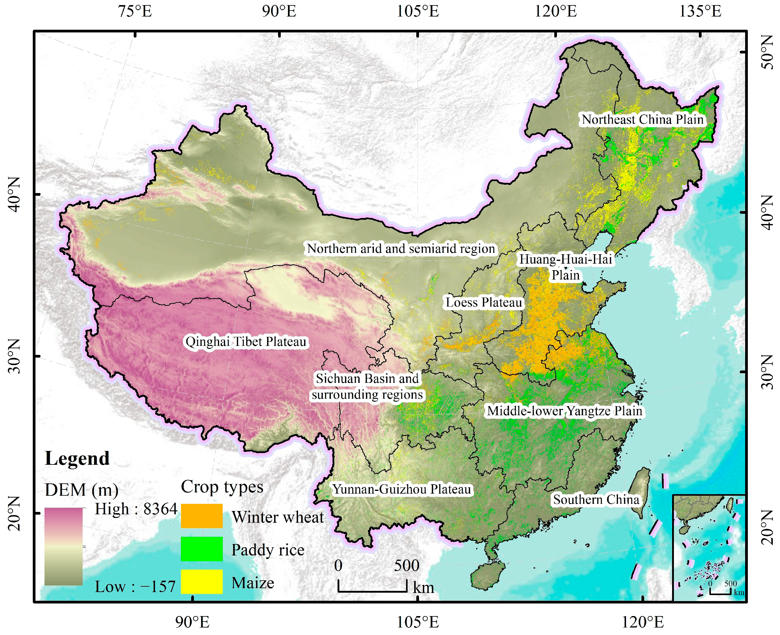
According to the characteristics of agricultural production environments and development orientations, previous researchers divided China into nine major agricultural regions (http://www.resdc.cn/, accessed on 1 May 2025): the Northeast China Plain (NEP), the Yunnan–Guizhou Plateau (YGP), the Northern Arid and Semiarid Region (NAS), Southern China (SC), the Sichuan Basin and Surrounding Regions (SBS), the Middle–Lower Yangtze Plain (MYP), the Qinghai–Tibet Plateau (QTP), the Loess Plateau (LP), and the Huang–Huai–Hai Plain (HHH). These regions reflect large-scale differences in climate, terrain, cropping systems, and dominant crop types. For example, the NEP and NAS are mainly characterized by single-cropping systems dominated by maize and wheat, the HHH supports a typical wheat–maize double-cropping rotation under flat terrain and moderate rainfall, whereas the MYP and SC are featured by humid climates and intensive rice-based multiple-cropping systems. Mountainous and plateau regions such as the YGP, SBS, LP, and QTP exhibit complex topography, fragmented cropland, and diverse cropping patterns (Figure 1).

Such traditional agricultural regionalization provides an important reference for understanding the spatial heterogeneity of China’s agro-ecosystems. However, these divisions are primarily established from the perspective of production conditions and resource endowment, and do not explicitly account for key constraints on remote sensing observation and crop-type identification, such as cloud contamination, terrain-induced radiometric distortion, and landscape fragmentation. As a result, they are not fully adequate for directly supporting large-scale, operational cropland and crop-type classification.

2.2. Data and Pre-Processing

2.2.1. Remote Sensing Datasets

Daily MOD09GA data from 2020 to 2024 is selected to calculate cloud cover conditions across different regions of the study area through overlay analysis. MOD09GA is a daily MODIS surface reflectance product with a spatial resolution of 1 km, and its state_1km Quality Assessment (QA) band provides pixel-level cloud information (https://ladsweb.modaps.eosdis.nasa.gov/, accessed on 1 May 2025). Cloud contamination was identified using the internal cloud algorithm flag (bit 10) in the state_1km QA band. Only valid MODIS observations flagged by the QA band were included in the analysis, while pixels affected by cloud contamination or invalid retrievals were excluded.

2.2.2. Land Cover and Land Use Datasets

The cropland data used in this study were derived from the WorldCover 10 m 2020 product released by the European Space Agency (ESA). This dataset was produced based on Sentinel-1 and Sentinel-2 imagery and includes 11 land cover types (forest, shrubland, grassland, cropland, built-up areas, bare land, snow and ice, open water, herbaceous wetland, mangroves, and moss). It has a spatial resolution of 10 m and an overall accuracy of 74.4% (https://esa-worldcover.org/, accessed on 1 May 2025).

Based on this ESA WorldCover dataset, cropland types were extracted, and indicators such as cropland area, cropland proportion, and cropland fragmentation were calculated at the county level. Further, to ensure the robustness of the first-tier validation, four mainstream 30 m resolution land use/land cover products for 2020 were selected for cross-comparison: CLCD, GlobeLand30, GLC-FCS30D, and CNLUCC. The selection of these specific datasets was predicated on their methodological diversity and data source independence.

While Landsat imagery serves as a primary input for most, their production pipelines vary significantly. CNLUCC (https://www.resdc.cn/, accessed on 20 May 2025) and GlobeLand30 (https://www.webmap.cn/, accessed on 20 May 2025) are characterized by substantial expert involvement, utilizing manual visual interpretation and human–computer interactive refinement, respectively, which ensures high thematic accuracy through expert knowledge. In contrast, CLCD and GLC-FCS30D are products of fully automated workflows; CLCD employs a random forest framework on the Google Earth Engine (GEE) platform (https://doi.org/10.5281/zenodo.4417810, accessed on 20 May 2025), while GLC-FCS30D utilizes a global spatiotemporal multispectral library with continuous change detection (https://data.casearth.cn/, accessed on 20 May 2025).

Crucially, these products maintain high independence from the primary ESA WorldCover (10 m) dataset used for indicator calculation. ESA WorldCover is uniquely driven by Sentinel-1 SAR and Sentinel-2 optical data, whereas the 30 m products are predominantly Landsat-based. Furthermore, the training and validation samples for each product are derived from disparate field surveys and independent reference libraries. This multi-source, multi-method ensemble effectively reduces the likelihood of correlated errors, providing a reliable, independent basis for verifying the spatial consistency of our cropland zoning.

2.2.3. Crop Datasets

The crop distribution data were obtained from the National Ecosystem Science Data Center (https://nesdc.org.cn/, accessed on 1 May 2025), which provides nationwide spatial distribution maps of maize, wheat, and rice. The spatial resolution of the maize and wheat data is 30 m, while that of the rice data is 10 m.

The cropping system data were derived from the Global Agro-Ecological Zones (GAEZ) dataset developed by the Food and Agriculture Organization of the United Nations (FAO) (https://gaez.fao.org/, accessed on 1 May 2025). The GAEZ dataset is based on the Agro-Ecological Zones (AEZ) methodology and evaluates agricultural resources and potentials across six thematic domains, which are Land and Water Resources, Agro-climatic Resources, Agro-climatic Potential Yield, Suitability and Attainable Yield, Actual Yields and Production, and Yield and Production Gaps. In this study, cropping system data with a spatial resolution of approximately 9 km were extracted from the Agro-climatic Resources theme.

To validate the zoning results, a total of 6555 validation samples covering winter wheat, maize, rice, and non-crop categories were collected in 2024 through visual interpretation of high-resolution remote sensing imagery and field surveys. The samples were spatially distributed in representative major production regions, with winter wheat samples mainly located in Shandong Province, maize samples in Heilongjiang Province, and rice samples in Guangdong and Jiangxi Provinces. These regions correspond to the dominant cropping areas of the three major cereals and are consistent with the phenological and planting patterns of the year used for constructing the second-tier crop zoning, ensuring temporal comparability between the validation data and the zoning results. Specifically, the dataset includes 930 wheat and 904 non-wheat samples, 1182 maize and 1139 non-maize samples, and 1200 rice and 1200 non-rice samples. These samples were used to evaluate the classification performance within the second-level major cereal crop zones by computing the Overall Accuracy (OA) and Kappa coefficient for winter wheat, maize, and rice, respectively.

2.2.4. Topographic Data

The topographic data used were obtained from the ASTER Global Digital Elevation Model (GDEM) released by NASA (https://www.earthdata.nasa.gov/, accessed on 1 May 2025), with a spatial resolution of 1 arc-second (approximately 30 m). After clipping and projection transformation, slope data were generated, maintaining a spatial resolution of 30 m.

2.2.5. Affiliated Data

The administrative boundary data were obtained from the official website of the National Geomatics Center of China (https://www.webmap.cn/, accessed on 1 May 2025). The dataset includes the administrative boundaries of all provinces, prefecture-level cities, and counties in mainland China for the year 2024.

3. Methods

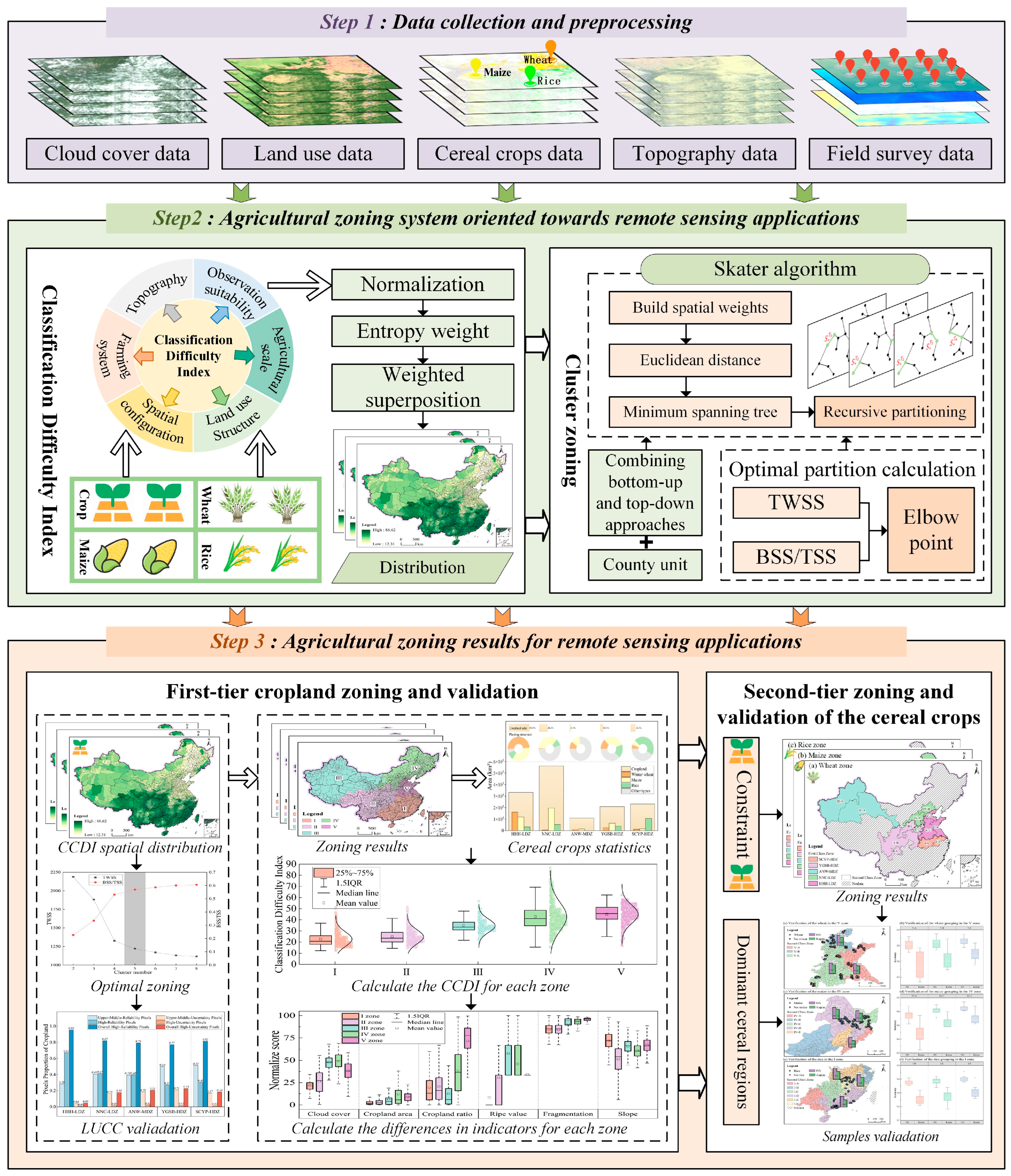
Considering the pronounced hierarchical structure of agricultural systems and the heterogeneity across crop types, a single-tier zoning scheme is insufficient to simultaneously support both regional-scale cropland monitoring and fine-scale monitoring of major cereal crops. Therefore, this study proposes a two-tier “cropland–major cereal crops” zoning framework. At the first tier, a macro-level division is established for cropland; at the second tier, a refined subdivision is conducted within each primary zone for major cereal crops. This design enables a unified framework to organize remote sensing applications across multiple spatial scales and monitoring targets. The remote-sensing-oriented agricultural classification difficulty zoning proposed in this study consists of three main steps (Figure 2).

First, to evaluate the implementation difficulty of large-scale agricultural remote sensing monitoring across different regions, this study developed a comprehensive indicator system that integrates indicators reflecting both agricultural cultivation heterogeneity and remote sensing observation variability. Multiple spatial indicators were derived to characterize key dimensions influencing classification difficulty feasibility. These include: remote sensing cloud frequency (representing observation suitability), total cropland area (agricultural scale), cropping proportion (land use structure), landscape fragmentation (spatial configuration), cropping intensity (farming system), and slope (topographic conditions). Collectively, these indicators form a multidimensional framework that captures both biophysical constraints and agricultural activity patterns, providing a systematic basis for subsequent remote sensing-based agricultural zoning.

Second, a zoning criterion was established based on key indicators that characterize remote sensing image acquisition capacity, along with the spatial distribution and morphology of cropland. An entropy weight method was applied to synthesize these indicators into a composite Cropland Remote-Sensing Classification Difficulty Index (CRCDI). Following this, the Skater algorithm, which is rooted in graph theory and enforces spatial constraints during clustering, was employed to perform regional delineation. This procedure generated the first-tier agricultural zoning for cropland, revealing the spatial heterogeneity of cropland classification difficulty in terms of cloud contamination frequency, terrain-induced radiometric and geometric distortions, and landscape fragmentation, which jointly determine the feasibility and reliability of large-scale remote sensing-based cropland mapping.

Finally, within each first-tier cropland zone, relevant indicators for the three major cereal crops (winter wheat, maize and rice) were selected as the basis for second-tier zoning. The entropy weight method was applied again to integrate these crop-specific indicators into a composite index, termed the Major Cereal Crops Remote-sensing Classification Difficulty Index (MCCRCDI). Subsequently, the Skater clustering algorithm was implemented to generate the second-tier agricultural subdivisions for these cereal crops. Through this procedure, a remote-sensing-oriented and hierarchically structured two-tier agricultural zoning framework, encompassing both cropland and major cereal crops, was systematically established.

3.1. Indicators for Remote-Sensing-Oriented Agricultural Zoning

In this study, agricultural remote sensing classification difficulty is conceptualized as the impediments encountered during remote sensing monitoring, resulting from the combined effects of limitations in data acquisition (e.g., persistent cloud cover), complexities in target identification (e.g., high cropland fragmentation or complex planting structures), and interference from background environmental conditions (e.g., rugged topography). Based on this conceptual framework and in consideration of the documented impacts of cloud cover and cropland characteristics on classification accuracy, six variables were selected as first-tier indicators for cropland zoning, including: cropland cloud cover frequency, cropland area, cropland proportion, cropland fragmentation, cropping intensity, and average cropland slope (

Table 1. Indicator system for the first-tier zoning.

Element Layer	Indicator Layer	Indicator Description	Effect Direction	Weight (%)
Remote sensing image availability	Cropland cloud cover frequency	Ratio of cloud-covered days to total days over cropland	Negative	14.126
Agricultural scale	Cropland area	Total area of cropland within the region	Positive	38.787
Land use structure	Cropland proportion	Ratio of cropland area to total regional area	Positive	23.421
Farming system	Cropping intensity	Frequency and rhythm of land use and planting within a year	Negative	13.521
Spatial configuration	Cropland fragmentation	Degree to which cropland is subdivided by other land-cover types	Negative	5.609
Topographic conditions	Cropland slope	Mean slope of cropland within the region	Negative	4.535

).

For the second-tier zoning of major cereal crops, six parallel indicators were adopted, measuring corresponding attributes specific to rice, wheat, and maize: cloud cover frequency over major cereal crops, major cereal crop area, major cereal crop proportion, major cereal crop fragmentation, cropping intensity, and average slope of major cereal crop fields (

Table 2. Indicator system for the second-tier zoning.

Element Layer	Indicator Layer	Indicator Description	Effect Direction	Weight (%)
Remote sensing image availability	Major cereal crop cloud cover frequency	Total area of major crop within the region	Negative	14.126
Agricultural scale	Major cereal crop area	Ratio of major crop area to total regional area	Positive	38.787
Land use structure	Major cereal crop proportion	Frequency and rhythm of land use and planting within a year	Positive	23.421
Farming system	Cropping intensity	Degree to which major crop is subdivided by other land-cover types	Negative	13.521
Spatial configuration	Major cereal crop fragmentation	Mean slope of major crop within the region	Negative	5.609
Topographic conditions	Major cereal crop slope	Total area of major crop within the region	Negative	4.535

). Subsequently, the entropy weight method was employed to integrate these indicators and generate the CRCDI and the MCCRCDI. Higher index values indicate greater difficulty in accurately identifying cropland or major cereal crops from remote sensing imagery, whereas lower values correspond to conditions more conducive to reliable detection.

The definitions and computational procedures for each indicator are detailed below:

(1) Cloud cover frequency: This indicator represents the proportion of days during which cropland or major cereal crops are obscured by clouds during MODIS satellite overpasses within the past five years, relative to the total number of observation days. To ensure national-scale comparability, a uniform multi-year observation window was adopted across all regions, with cloud frequency intended to characterize long-term observation opportunity constraints for optical remote sensing. It reflects the extent to which remote sensing spectral information is affected by cloud-induced noise, thereby directly influencing the accessibility of agricultural information. As such, it serves as a key parameter for evaluating the difficulty of agricultural remote sensing classification. The calculation formula is as follows:

$$CN=\sum _{\mathrm{i}=1}^{\mathrm{n}}Cloud\_day/\sum _{i=1}^{n}Day$$

(1)

where $CN$ denotes the five-year average proportion of cloud-covered days, $Cloud\_day$ indicates whether a given day during the growing season is obscured by clouds, and $Day$ represents the total number of days in the growing season.

(2) Cropland area and proportion: Cropland area refers to the total area of cropland within a region, reflecting the overall scale of agricultural production; cropland proportion represents the ratio of cropland area to the total regional area, indicating the degree of cropland concentration. A higher cropland proportion implies greater spectral homogeneity of land cover, which facilitates remote sensing identification and information extraction, thereby reducing classification difficulty. These indicators were derived from the cropland class of the ESA WorldCover dataset.

(3) Cropping intensity: Cropping intensity in this study refers to the multiple cropping index, which characterizes the number of crop cycles on the same cropland within one year and thus reflects the frequency of land use and the temporal periodicity of vegetation growth. It directly affects the seasonal dynamics of vegetation indices and spectral trajectories, thereby influencing the difficulty of remote sensing-based crop discrimination. The multiple cropping index was derived from the GAEZ dataset and treated as a classified variable. This classified indicator was used to quantify surface phenological periodicity and temporal spectral variability associated with different cropping systems and to characterize their impacts on remote sensing monitoring and classification performance.

(4) Cropland and major cereal crop fragmentation: Cropland or major cereal crop fragmentation refers to the degree to which cropland or major cereal crop areas are spatially subdivided by other land use types, reflecting the spatial connectivity and shape complexity of cropland or major cereal crop patches. Highly fragmented cropland or major cereal crop patterns tend to cause remote sensing classification errors such as “same object, different spectra” and “different objects, similar spectra,” thereby increasing the difficulty of agricultural remote sensing classification. The calculation formula is as follows:

$$P_s={\displaystyle \frac{\sum C_i}{4\times \sum A_i}}$$

(2)

where $P_s$ represents the fragmentation index, $\sum C_i$ denotes the total perimeter of all patches, and $\sum A_i$ denotes the total area of all patches. Specifically, $P_s$ was calculated at the county level using 10-m resolution cropland and major cereal crop data. For each county, the total area and total perimeter of all cropland or crop-specific pixels were aggregated to derive a single $P_s$ value, representing the overall spatial fragmentation within the administrative unit. Patch connectivity was defined based on raster adjacency, and a consistent patch definition and spatial resolution were applied nationwide to ensure comparability across regions.

(5) Mean slope: Topographic relief affects the spectral homogeneity of land surfaces, as variations in slope and aspect can alter reflectance characteristics and produce terrain-induced shadows, thereby introducing noise into spectral information and reducing the accuracy of remote sensing classification. In this study, the mean slope within cropland or major cereal crop distribution areas was used to characterize the influence of topographic factors.

3.2. Methodology for Remote-Sensing-Oriented Agricultural Zoning

3.2.1. Agricultural Zoning Based on the Skater Algorithm

The Skater algorithm is a hierarchical clustering method that uses under spatial constraints. It connects spatially adjacent objects through a Minimum Spanning Tree (MST) and progressively merges regions that are both spatially contiguous and highly similar, ultimately forming several spatially continuous and internally homogeneous clusters [23,24,25]. In this study, the spatially explicit constraints and hierarchical clustering mechanism of the Skater algorithm were used to construct a hierarchical zoning framework for agricultural remote sensing monitoring. This framework ensures spatial continuity while effectively reducing regional heterogeneity.

Specifically, at the macro level, spatially continuous first-tier agricultural zones were delineated based on cropland characteristics. These zones then served as spatial constraints for the refined second-tier subdivision targeting major cereal crops, thereby establishing a scale-progressive and hierarchically structured two-tier “cropland–major cereal crops” zoning system. To ensure the scientific validity and comparability of the zoning results, the optimal number of clusters was determined using a best partitioning method. Based on the cluster centroids, classification difficulty levels were subsequently classified, providing technical support for spatially explicit agricultural remote sensing monitoring and regional management.

The optimal number of clusters was identified using two clustering evaluation metrics: the Total Within-Cluster Sum of Squares (TWSS) and the ratio of the Between-Cluster Sum of Squares to the Total Sum of Squares (BSS/TSS). The elbow method was subsequently applied to determine the final cluster count. The selected cluster number was further verified through comparative statistical analysis of intra-zone heterogeneity and inter-zone separability, ensuring the robustness of the final zoning scheme.

TWSS quantifies the internal compactness of clusters (Equation (3)). A smaller TWSS indicates tighter grouping of samples within clusters, reflecting higher clustering quality. The BSS/TSS ratio, ranging from 0 to 1 (Equations (4)–(6)), measures the separation between clusters: a value of 0 corresponds to complete overlap among categories (poorest clustering), while a value of 1 indicates perfect separation (optimal clustering) [11,26].

The basic principle of the elbow method is that as the number of clusters (k) increases, TWSS gradually decreases while BSS/TSS increases. When further increases in k yield only marginal improvements in clustering quality, the corresponding inflection point—known as the “elbow point”—is identified as the optimal number of clusters for the zoning scheme.

$$TWSS=\sum _{j=1}^k\sum _{x_i\in C_j}{\Vert x_i-{\mu }_j\Vert }^2$$

(3)

In these equations, TWSS measures the degree of dispersion within clusters. $x_i$ represents individual sample units, $k$ is the number of clusters, and ${\mu }_j$ is the centroid of cluster Cⱼ.

$$TSS=\sum _{i=1}^n{\Vert x_i-\mu \Vert }^2$$

(4)

$$BSS=TSS-TWSS$$

(5)

$${\displaystyle \frac{BSS}{TSS}}=1-{\displaystyle \frac{TWSS}{TSS}}$$

(6)

TSS reflects the overall variability of the dataset, where $\mu$ denotes the mean of the entire dataset. BSS measures the degree of separation among different clusters. The ratio BSS/TSS indicates the proportion of between-cluster variance relative to the total variance.

3.2.2. First-Tier Zoning Scheme

In this study, counties were used as the basic zoning units, and the first-tier agricultural zoning indicator system was constructed according to remote sensing monitoring requirements. First, all indicators were standardized using the min–max normalization method (Equations (7) and (8)), and indicator weights were calculated using the entropy weighting method. A comprehensive weighting calculation was then used to derive the CRCDI.

Subsequently, the Skater algorithm was applied for spatially constrained clustering. A first-order Queen contiguity spatial adjacency graph was constructed among county units, and Euclidean distance based on standardized indicators was used to generate the MST. The edges with the highest dissimilarity were iteratively removed, resulting in spatially contiguous and internally homogeneous clusters. The Skater clustering and spatial optimization procedures were implemented in GeoDa (version 1.2.2), following its default MST construction and pruning strategy, whereby edges with the largest dissimilarity values were iteratively removed until the predefined number of clusters was reached. The optimal number of clusters was determined using the optimal partitioning method, and spatial optimization of the resulting zones was used. Finally, the centroid value of the CRCDI for each zone was calculated and ranked to assign difficulty levels, forming the first-tier agricultural zoning scheme.

During the post-zoning optimization stage, strict adherence to the principle of regional contiguity was maintained. Discrete county units forming “enclaves” were removed to ensure spatial continuity of each zone. Small or isolated agricultural regions and special topographic units such as islands were merged with adjacent dominant zones according to spatial proximity and the “majority rule” principle. This procedure preserved the spatial coherence of agricultural characteristics while avoiding fragmentation in the zoning results caused by local anomalies.

$$y_i=\left(x_j-x_{jmin}\right)/(x_{jmax}-x_{jmin})$$

(7)

$$y_i=\left(x_{jmax}-x_j\right)/(x_{jmax}-x_{jmin})$$

(8)

where $y_i$ is the standardized value of $x_j$; $x_j$ is the initial value of the indicator $j$; $x_{jmin}$ and $x_{jmax}$ are the minimum and maximum values of index $j$ respectively.

3.2.3. Second-Tier Zoning Scheme

Building upon the first-tier zoning scheme, we further conducted a second-tier subdivision focusing on the three major cereal crops—rice, wheat, and maize. First, the MCCRCDI was constructed separately through min–max normalization and entropy-based weighting. Using the boundaries of the first-tier zones as spatial constraints, county-level units containing cultivation of the major cereal crops were identified. The same Skater spatial clustering algorithm as in the first-tier zoning was then applied, based on Queen contiguity relationships and Euclidean distance measures, to perform spatially constrained clustering of these crop-producing county units.

Next, the optimal number of clusters was determined using the optimal cluster partitioning method, and post-zoning spatial optimization was conducted following the same procedure as in the first-tier scheme to address irregular or isolated spatial units. Finally, the centroid values of the MCCRCDI within each zone were calculated and ranked to assign zonal difficulty levels. The resulting second-tier zoning scheme not only preserves the computational efficiency of the Skater algorithm but also refines the spatial differentiation of remote sensing monitoring suitability across different major cereal crops, thereby providing a more detailed spatial decision-making basis for the formulation of agricultural remote sensing observation strategies.

3.3. Accuracy Assessment

3.3.1. Accuracy Evaluation for the First-Tier Zoning Scheme

For the remote-sensing-oriented first-tier agricultural zoning, a quantitative evaluation framework was established based on pixel-level classification reliability and classification uncertainty. The evaluation process involved the following steps: first, four representative land use/cover change(LUCC) products—CLCD, GlobeLand30, GLC-FCS30D, and CNLUCC—were selected, and their cropland masks were overlaid for comparative analysis. Then, for each zoning unit, the classification results of cropland pixels across the four products were examined, and the proportion of pixels consistently identified as cropland was calculated.

Pixels classified as cropland by all four products (i.e., only one land-cover category after overlay) were defined as High-Reliability pixels. Pixels showing two land-cover categories after overlay, corresponding to cases where three products identified cropland and one product assigned a different land-cover type, were defined as Upper-Middle-Reliability pixels. Pixels exhibiting three land-cover categories after overlay, indicating that only two products classified the pixel as cropland while the remaining two corresponded to two different non-cropland types, were defined as Upper-Middle-Uncertainty pixels. Pixels showing four distinct land-cover categories after overlay, meaning that only one product identified cropland and the other three assigned three different non-cropland types, were defined as High-Uncertainty pixels. Accordingly, Overall High-Reliability Pixels were defined as the combination of the High-Reliability and Upper-Middle-Reliability classes, whereas Overall High-Uncertainty Pixels were defined as the combination of the High-Uncertainty and Upper-Middle-Uncertainty classes. This categorization enabled a quantitative assessment of the internal consistency and spatial reliability of the zoning results.

3.3.2. Accuracy Evaluation for the Second-Tier Zoning Scheme

For the second-tier zoning of major cereal crops, an evaluation approach based on field and visually interpreted sample validation was employed to assess the accuracy of crop classification within each zoning unit. Specifically, the spatial distribution maps of winter wheat, maize, and rice provided by the National Ecosystem Science Data Center of China were adopted as the reference classification products. These datasets were generated using remote sensing-based classification methods and have reported overall accuracies exceeding 80%, thereby providing a reliable basis for validation. Sample point data were used to evaluate the classification accuracy within each second-tier cereal crop zone by calculating the OA and the Kappa coefficient, which respectively quantify the overall correctness and the agreement beyond chance.

Within the extent of the first-tier cropland zones, the spatial distribution of planting areas for each major cereal crop was analyzed, and the zone with the largest planting area for each cereal crop was selected as the representative region for validation and analysis. The computation of OA and Kappa coefficients followed standard procedures for accuracy assessment in remote sensing classification [27].

3.4. Comparison of Clustering Methods and Rationale for Method Selection

To achieve a reasonable balance between attribute homogeneity and spatial contiguity, four representative zoning approaches were systematically compared: (1) Kmeans (entropy-weighted, without spatial constraints), (2) Redcap (entropy-weighted, with spatial constraints), (3) Skater (equal-weighted, with spatial constraints), and (4) the proposed entropy-weighted Skater method (with spatial constraints). This experimental design allows the simultaneous evaluation of the effects of spatial constraints and indicator weighting schemes on zoning performance.

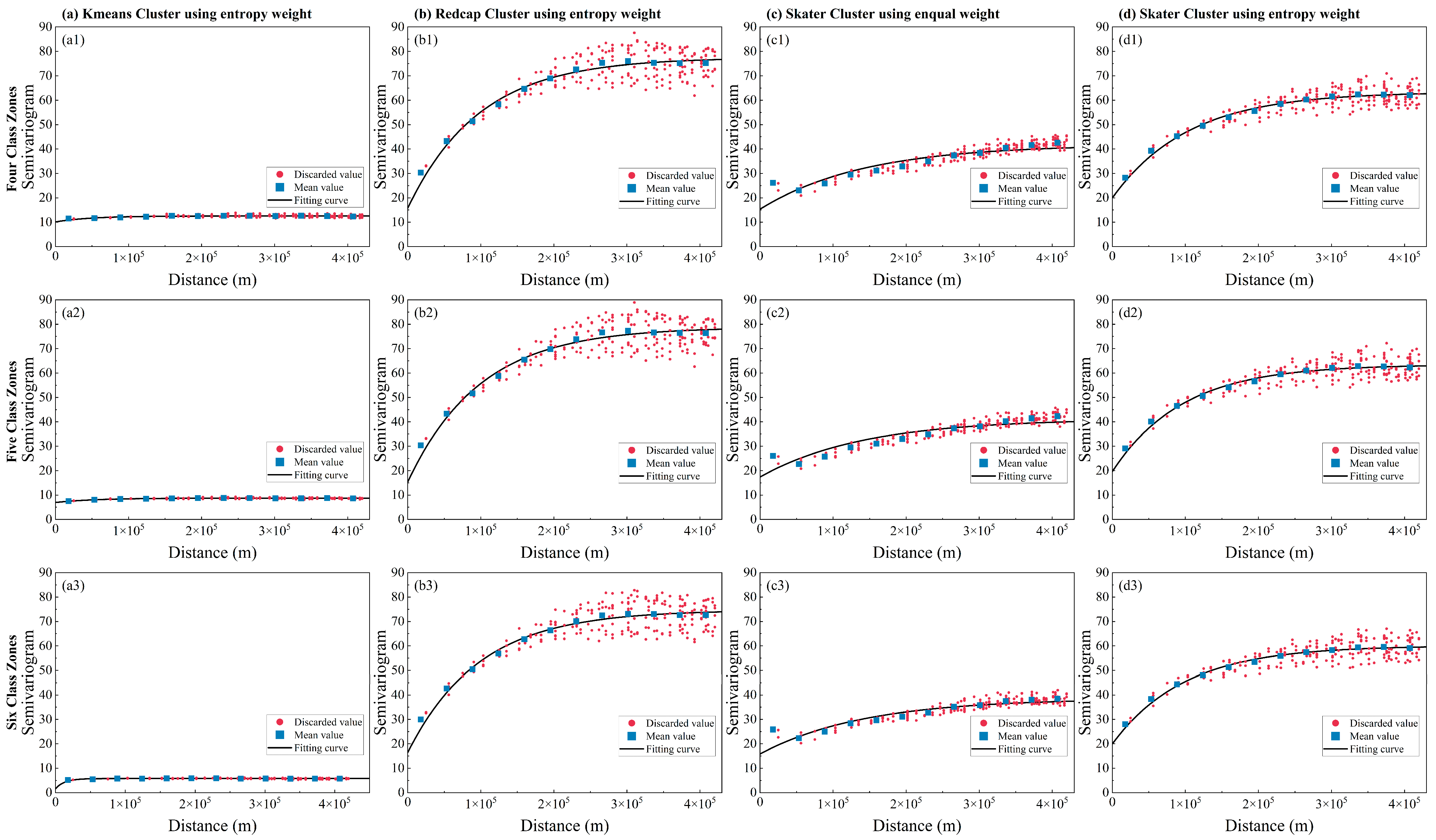
The performance of different zoning schemes was evaluated from three complementary aspects: (1) Statistical separability, assessed using the Kruskal–Wallis test to examine whether inter-zone differences in the CRCDI are significant. (2) Spatial explanatory power, quantified by the residual Moran’s I index to measure how well each method captures the spatial dependence of CRCDI. (3) Spatial structural stability, analyzed using semivariograms to characterize within-zone heterogeneity and its dominant spatial scales. In this study, semivariograms are used as an intuitive tool to characterize the internal spatial structure of each zoning scheme. The sill represents the overall magnitude of within-zone variance, with lower sill values indicating higher internal homogeneity and structural stability. The range denotes the spatial distance over which spatial autocorrelation persists, reflecting the dominant spatial scale at which zoning patterns remain coherent; a reasonable and stable range suggests that the zoning captures meaningful regional structures rather than local noise.

Based on this multi-criteria evaluation framework, the clustering methods were compared in terms of their ability to balance attribute discrimination, spatial contiguity, and internal structural coherence.

4. Results and Analysis

4.1. First-Tier Cropland Zoning and Validation

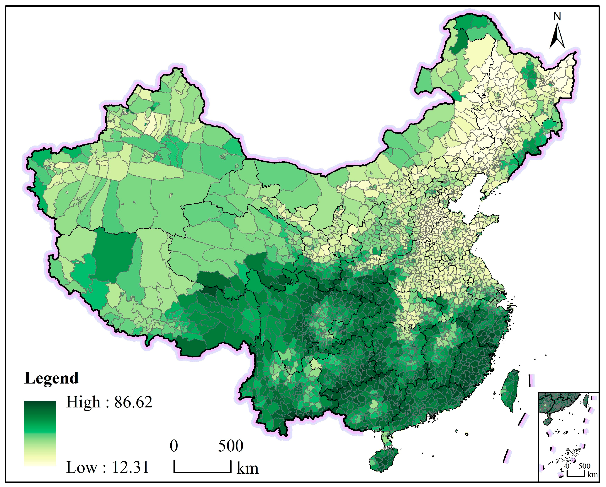
The CRCDI, calculated based on the entropy weight method and the indicator system for the first-tier zoning, is presented in Figure 3. Overall, the CRCDI reveals a clear south–north gradient in cropland classification difficulty, with the highest difficulty concentrated in humid, topographically complex southern China and the lowest difficulty in the flat, dry, and intensively cultivated plains of northern China.

From the spatial pattern, areas with relatively low difficulty are predominantly distributed in northern China, particularly across the HHH and the NEP. These regions represent typical large-scale, mechanized agricultural zones, characterized by extensive alluvial plains, flat terrain, and large, contiguous cropland patches. Moreover, owing to strong precipitation seasonality, cloud cover during the main growing season is relatively limited, allowing the acquisition of high-quality optical remote sensing imagery and resulting in low CRCDI values.

In contrast, the NAS and the QTP, although containing less cropland overall, exhibit moderate classification difficulty. Their arid climate and sparse cloud cover provide favorable observation conditions, but cropland is mainly distributed in narrow river valleys and oasis systems, leading to fragmented spatial patterns and thus a medium level of CRCDI.

The highest classification difficulty is observed in southern China, where complex terrain and persistent cloud contamination jointly constrain remote sensing-based cropland identification. This region is dominated by low mountains and hills, with cropland that is highly fragmented and irregular in shape. In addition, the influence of the East Asian monsoon results in a long rainy season and frequent cloud cover, substantially reducing the availability of usable optical imagery and yielding the highest CRCDI nationwide.

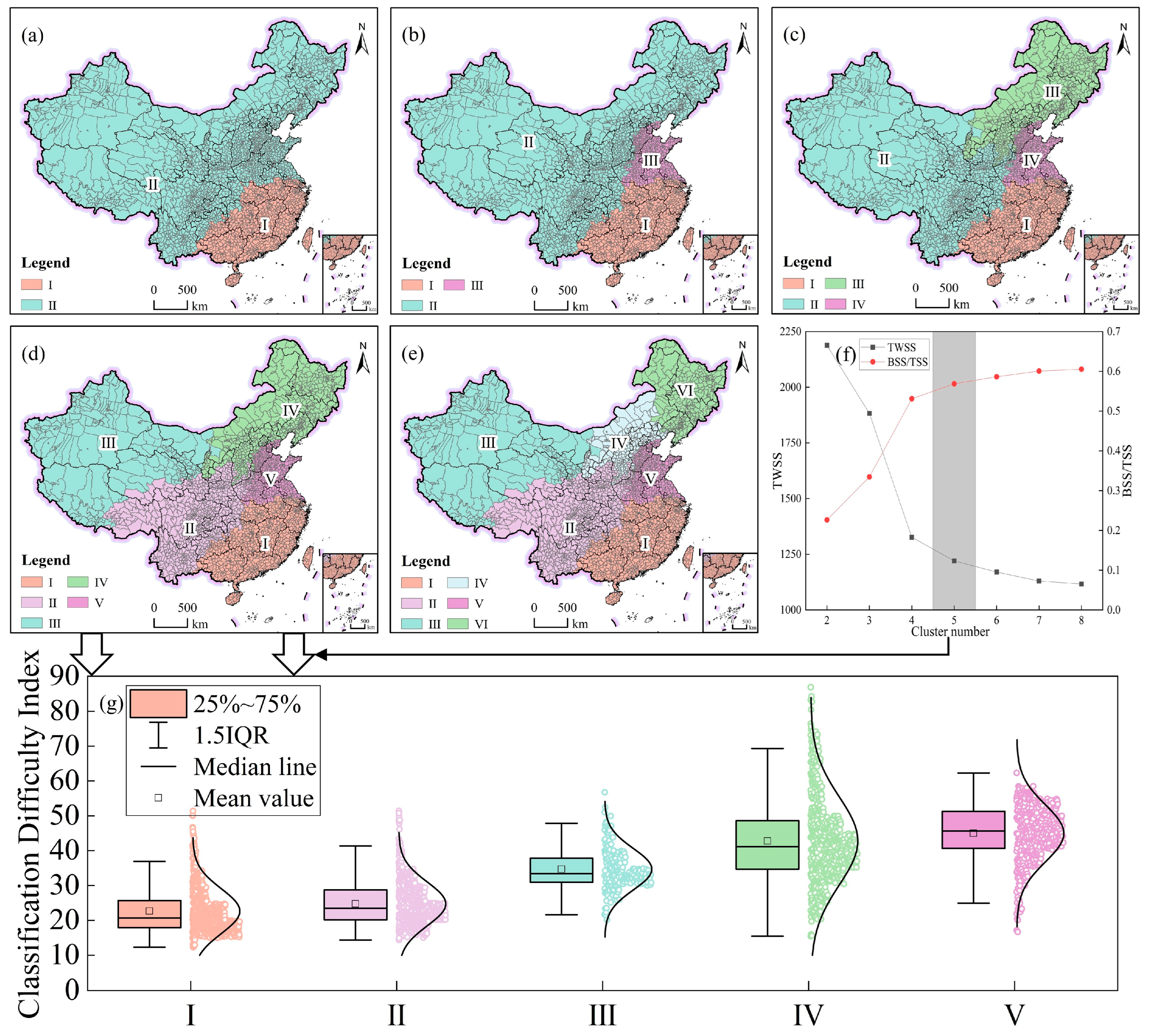
Based on the CRCDI, the Skater spatial clustering results (Figure 4) indicate that five clusters provide the optimal first-tier zoning scheme. As the number of clusters increases, TWSS decreases continuously while BSS/TSS increases. When the cluster number reaches five, the reduction in TWSS becomes marginal and the increase in BSS/TSS slows markedly, forming a clear “elbow point” with BSS/TSS exceeding 60%. This demonstrates that a five-zone solution achieves the best trade-off between within-zone homogeneity and between-zone separability. Accordingly, China is divided into five first-tier cropland zones, ordered from high to low classification difficulty as Categories I–V, with larger category numbers indicating lower CRCDI.

Zone I is defined as the South China and Yangtze Plain High Difficulty Zone (SCYP-HDZ), located in southeastern China and encompassing the middle–lower Yangtze River Plain, the Lingnan region, as well as offshore islands such as Hainan and Taiwan. This zone is characterized by persistently high cloud cover and an extended rainy season, resulting in substantially lower optical-image availability than the national average. In addition, cropland in coastal hilly areas is highly fragmented, leading to the highest overall CRCDI.

Zone II, the Yunnan–Guizhou Plateau–Sichuan Basin High Difficulty Zone (YGSB-HDZ), lies in southwestern China and includes the YGP, SBS, and the southeastern margin of the QTP. The region is dominated by mountains, plateaus, and basins, with limited plains and highly dispersed, fragmented cropland. Combined with frequent cloud coverage, these characteristics maintain the zone at a high CRCDI.

Zone III, the Arid Northwest Moderate Difficulty Zone (ANW-MDZ), mainly covers Xinjiang, the QTP, and western Inner Mongolia. Although the region receives very little precipitation and has low cloud frequency—conditions conducive to stable optical observations—cropland is largely confined to river valleys and oasis systems, exhibiting pronounced spatial patchiness. As a result, the CRCDI falls within the moderate range.

Zone IV, the Northeast and North China Margin Low Difficulty Zone (NNC-LDZ), encompasses the three northeastern provinces and eastern Inner Mongolia. The region experiences relatively low cloudiness and features extensive, contiguous cropland in plain areas, ensuring high-quality and stable remote sensing imagery and therefore a lower CRCDI.

Zone V, the Huang-Huai-Hai Plain Low Difficulty Zone (HHH-LDZ), is situated in northern China and covers the HHH and the Shandong Peninsula. With flat terrain, highly consolidated cropland, and excellent optical-image availability, this zone exhibits the lowest CRCDI nationwide.

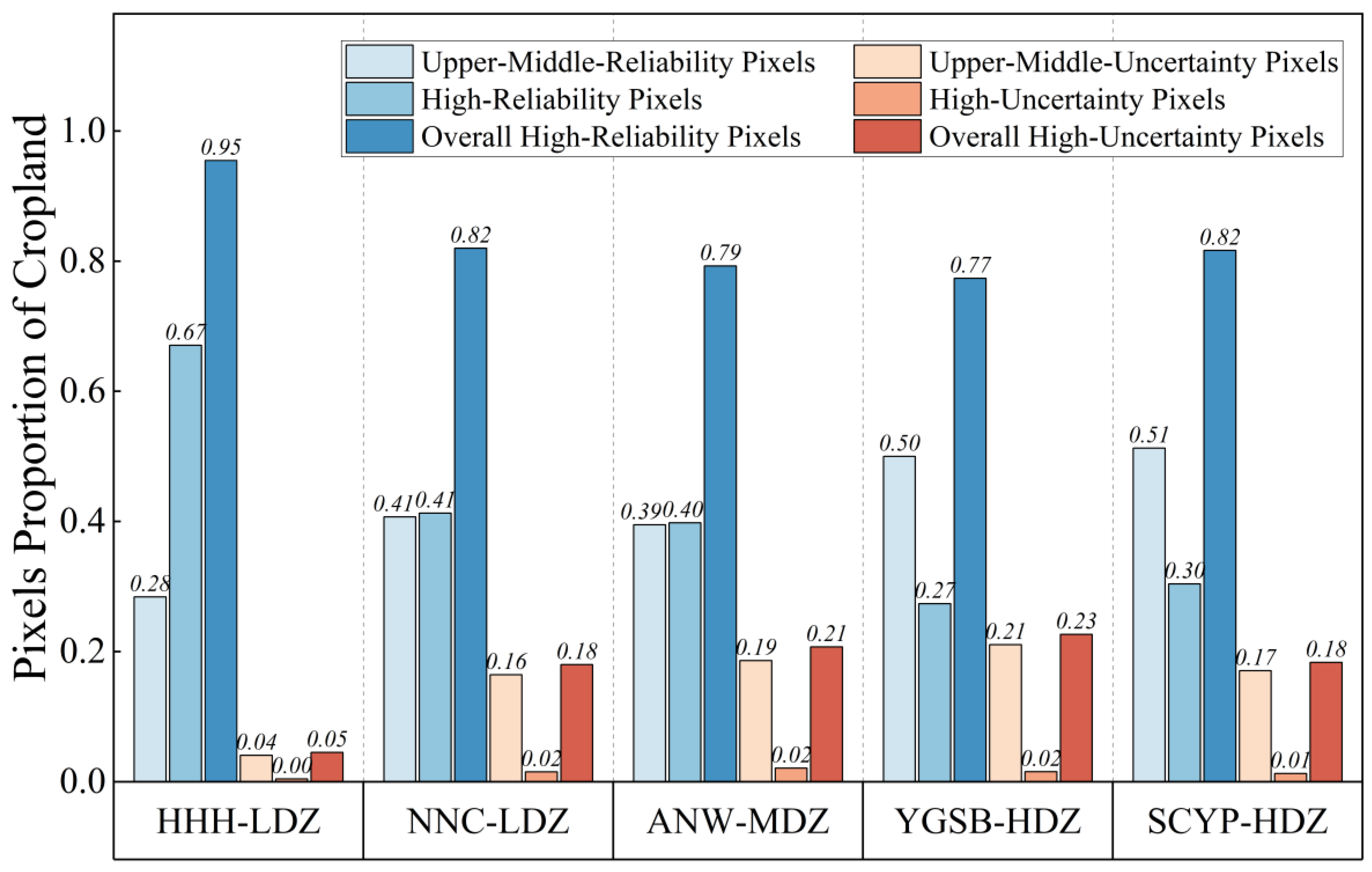
Overall, the uncertainty patterns derived from multi-source LUCC products are highly consistent with the CRCDI-based zoning, indicating that the first-tier zones effectively capture the spatial differentiation of cropland identification reliability. The reliability and uncertainty of cropland identification across the first-tier agricultural zones were evaluated using the four LUCC products (Figure 5). Overall, the spatial distribution of High-Uncertainty pixels closely corresponds to the difficulty levels defined by the zoning based on the CRCDI, thereby further validating the reliability of the zoning results.

The proportion of High-Reliability pixels varies substantially across zones. The HHH-LDZ exhibits the highest High-Reliability ratio, indicating the most stable cropland identification performance. In contrast, the YGSB-HDZ shows the lowest proportion, with the remaining zones following an ordered decline consistent with the transition from low-difficulty to high-difficulty zones.

In terms of High-Uncertainty pixels, the YGSB-HDZ and the ANW-MDZ show markedly higher proportions than the other zones, reflecting the combined effects of complex terrain, fragmented cropland, and suboptimal observation conditions. In contrast, the HHH-LDZ has the lowest uncertainty level, further confirming that flat terrain, large field sizes, and favorable atmospheric conditions jointly enhance cropland mapping stability.

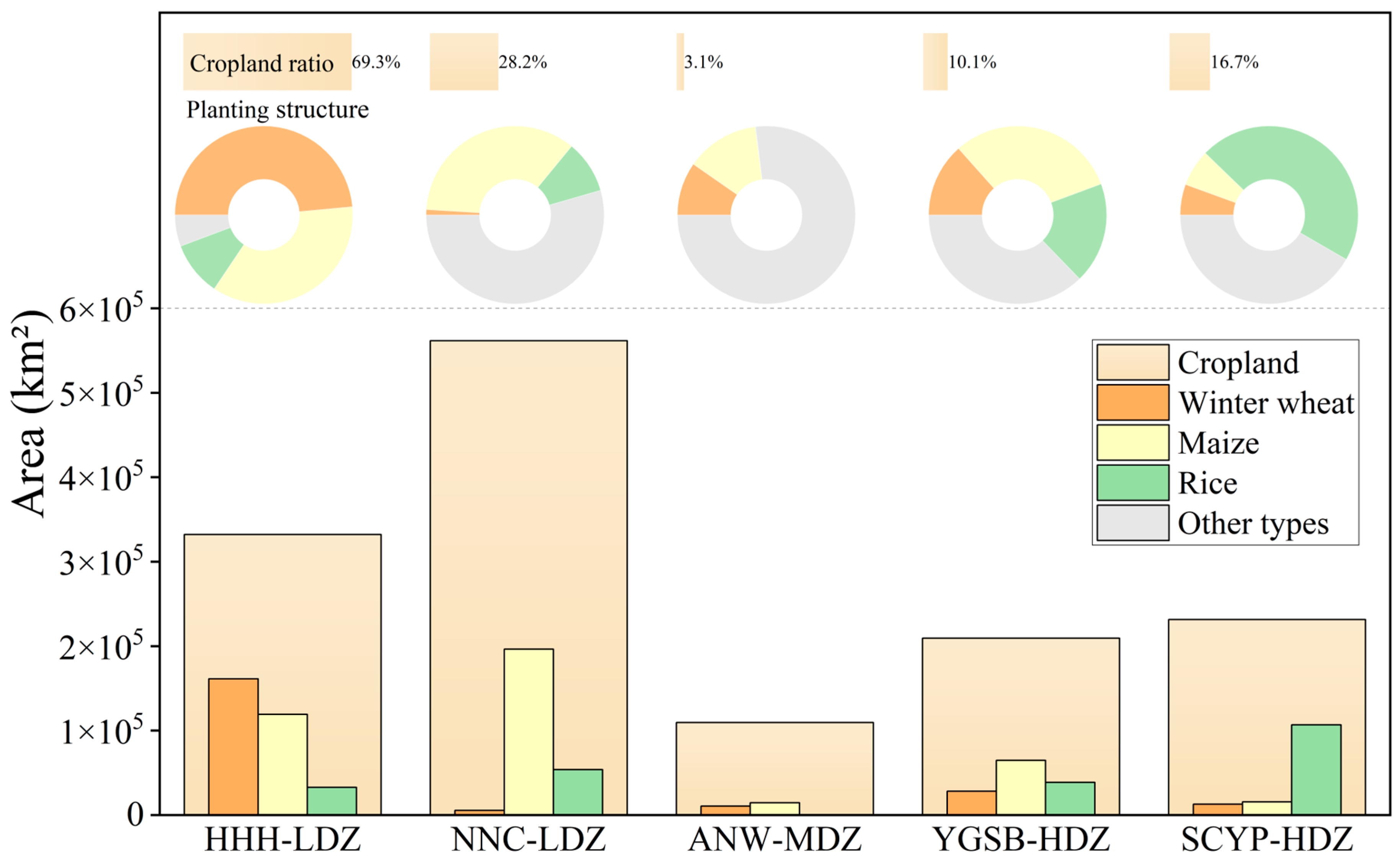
The first-tier zones are not only differentiated by CRCDI, but also by pronounced contrasts in cropland extent and dominant cropping systems, revealing a clear coupling between production geography and observation conditions (Figure 6). Significant differences in cropland scale and cropping structure are observed across the zones. The HHH-LDZ contains the largest share of national cropland, followed by the NNC-LDZ, whereas the ANW-MDZ has the smallest proportion due to its arid environment and oasis-type agricultural pattern.

Major cereal crops account for more than 50% of total cropland area in all zones, with the HHH-LDZ reaching as high as 95%, highlighting its role as China’s core grain-producing region. The three major cereal crops exhibit distinct spatial preferences: winter wheat is mainly concentrated in the HHH-LDZ, maize dominates the NNC-LDZ, and rice is primarily distributed in the SCYP-HDZ. These zonal differences in cropping structure further underpin the necessity of implementing differentiated, crop-specific remote sensing classification strategies within the proposed two-tier zoning framework.

4.2. Second-Tier Zoning and Validation of the Major Cereal Crops

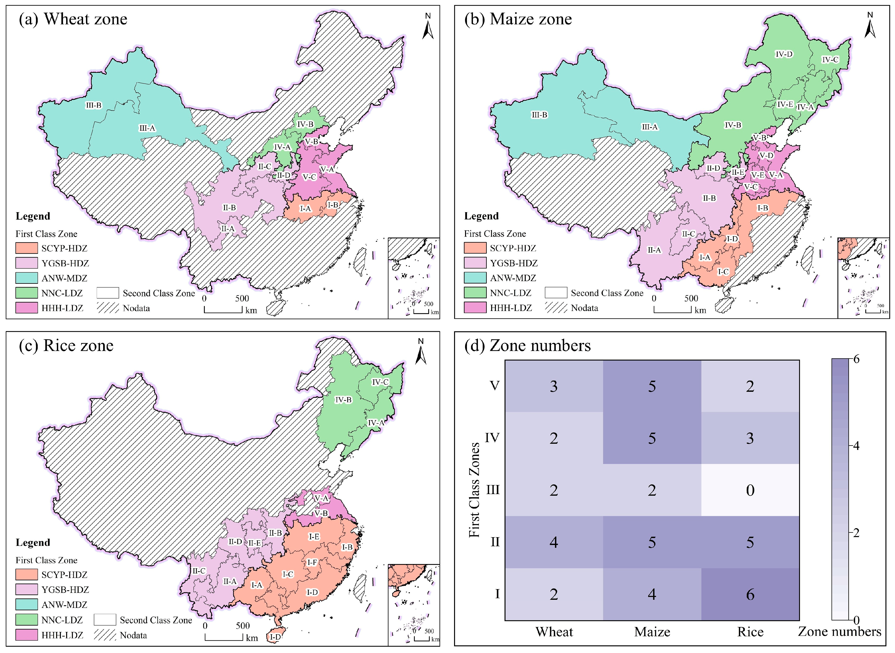
Building upon the first-tier zones and incorporating the spatial distributions of the three major cereal crops together with the second-tier indicator system, the MCCRCDI were separately calculated for rice, wheat, and maize. Based on these indices, second-tier zones for major cereal crops were delineated using the Skater clustering algorithm (Figure 7). Under the spatial constraints imposed by the first-tier zoning framework, the second-tier zones were encoded alphabetically from A to F according to descending classification difficulty, with A representing the highest difficulty and F the lowest.

Winter wheat is primarily distributed in central China, with the highest concentration occurring within the HHH-LDZ, while appearing only sparsely in other zones. Maize is the most widely cultivated crop nationwide, present in all first-tier zones; among them, the HHH-LDZ and NNC-LDZ have the largest maize-growing areas and consequently the most second-tier subdivisions. Rice cultivation is mainly concentrated in southern China and the northeastern region, covering three first-tier zones: the NNC-LDZ, YGSB-HDZ, and SCYP-HDZ. Marked differences in classification difficulty are observed across these regions. Notably, within the SCYP-HDZ, the high internal diversity of terrain types results in rice-growing areas being further partitioned into six second-tier zones, reflecting the pronounced spatial heterogeneity of monitoring conditions within this region.

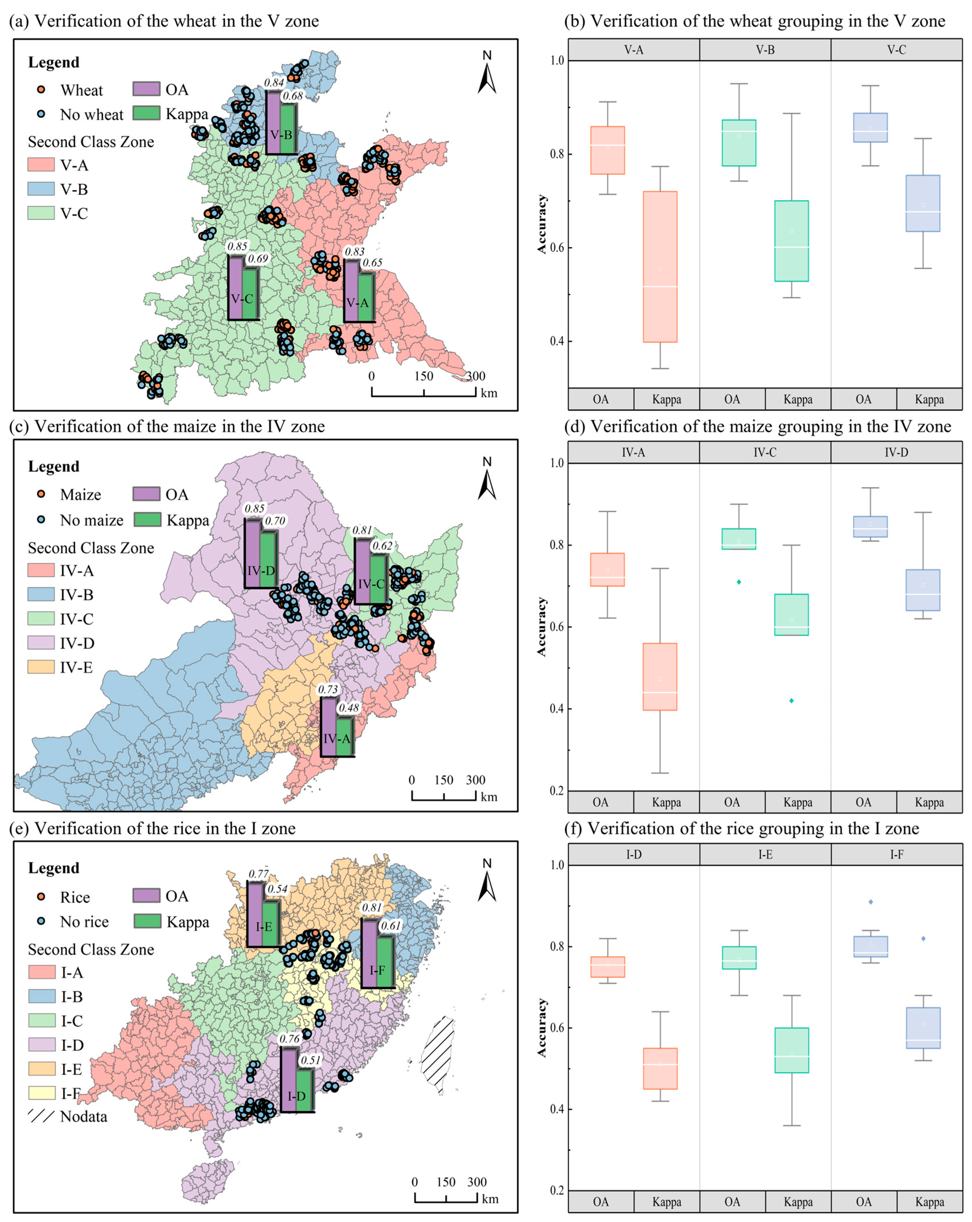
After obtaining the second-tier zoning results for major cereal crops, we further selected the first-tier zones with the largest crop-dominant planting areas—based on the statistics in Figure 6—to conduct validation. This approach allows evaluation of the monitoring suitability and discriminative capacity of the second-tier zones across different regions. Specifically, winter wheat second-tier zones were validated within the HHH-LDZ, maize second-tier zones within the NNC-LDZ, and rice second-tier zones within the SCYP-HDZ.

Within the HHH-LDZ, the OA values of winter wheat second-tier zones A, B, and C were 0.83, 0.84, and 0.85, respectively, with corresponding Kappa coefficients of 0.65, 0.68, and 0.69 (Figure 8). The three zones exhibited relatively stable accuracy levels, with Zone A showing slightly lower accuracy, consistent with its higher classification difficulty within the second-tier zoning scheme.

Within the NNC-LDZ, the OA values for maize second-tier zones A, C, and D were 0.73, 0.81, and 0.85, respectively, and the corresponding Kappa coefficients were 0.48, 0.62, and 0.70. Accuracy varied considerably across the zones. Zone A exhibited the lowest accuracy, while Zones C and D demonstrated higher performance, indicating that the second-tier zoning effectively captures the gradient of classification difficulty in this region.

Within the SCYP-HDZ, the OA values for rice second-tier zones D, E, and F were 0.76, 0.77, and 0.81, respectively, with Kappa coefficients of 0.51, 0.54, and 0.61. Zone F yielded the highest accuracy, whereas Zones D and E showed similar values, reflecting the spatially heterogeneous classification performance associated with the complex terrain and climatic conditions in southern China.

Across the three crop types, rice in the SCYP-HDZ exhibited significantly lower OA compared with winter wheat in the HHH-LDZ and maize in the NNC-LDZ. This pattern aligns well with the classification difficulty distribution revealed by the second-tier zones, further demonstrating that persistent cloudy–rainy weather and fragmented cropland structures in southern China substantially constrain the accuracy of remote sensing-based agricultural classification.

5. Discussion

5.1. Advantages and Limitations

5.1.1. Contributions and Advantages

The main contributions of this study lie not in producing another zoning map, but in clarifying why and where cropland and crop-type classification becomes unreliable at the national scale, and in translating this understanding into an operationally meaningful zoning logic.

(1) The study conceptually reframes agricultural zoning from a production-oriented paradigm to an observation-oriented paradigm. Unlike traditional agro-ecological regionalizations driven mainly by climate, soils, and cropping systems, the proposed two-tier framework explicitly takes Earth-observation constraints—particularly cloud contamination [16,28], terrain-induced signal distortion, field fragmentation, and phenological heterogeneity—as the organizing principle. This demonstrates that the spatial heterogeneity of classification difficulty is an emergent property of the coupled atmosphere–land–crop–sensor system rather than a simple reflection of natural geography.

(2) The study establishes a methodological framework that couples an interpretable classification difficulty index with spatially constrained regionalization. By integrating the entropy-weighted ARCDI with the Skater algorithm, the resulting zones are forced to be both geo-graphically contiguous and internally homogeneous in terms of key controlling factors, including cloud frequency, topographic complexity, cropland fragmentation, and cropping intensity. This design ensures that each zone corresponds to a comparable level and mechanism of classification difficulty, rather than being defined solely by statistical similarity or administrative boundaries. The framework thus provides a generalizable approach for constructing difficulty-oriented, spatially coherent regions in large-scale land-cover and crop-type mapping tasks.

(3) The study further provides an operational basis for zone-specific and task-oriented crop classification strategies. Instead of applying a uniform national model, the derived zones enable stratified algorithm design and sensor configuration: SAR–optical data fusion and spatiotemporal gap-filling can be prioritized in persistently cloudy and highly fragmented landscapes, whereas high-frequency optical observations and phenology-based classifiers are more suitable in flat, homogeneous plain regions. Such zoning-guided differentiation directly supports geo-graphically adaptive large-scale crop mapping and acreage estimation, improving both efficiency and robustness in operational applications.

5.1.2. Limitations

The limitations of this study are primarily reflected in the following two aspects:

(1) The evaluation of zoning accuracy is constrained by the quality of validation data. This study employs the consistency among multiple land-use products as an indicator of cropland identification reliability. However, the classification errors and systematic biases inherent to these products introduce uncertainty into the consistency-based evaluation. Differences among products in terms of imaging timing, spatial resolution, classification systems, and algorithms—particularly the handling of “mixed pixels” and “boundary croplands” [29,30,31]—may lead to biased assessments of classification difficulty.

In the second-tier zoning, the spatial extent of validation samples is geographically limited, which affects the comprehensiveness of zonal accuracy evaluation. Although the available samples are mainly distributed in representative major production regions, they do not fully cover all zones nationwide. As a result, the current validation evidence primarily supports the effectiveness of the proposed framework within the sampled regions, and caution is required when extrapolating the results to underrepresented areas with distinct agro-environmental conditions. Given the high cost of large-scale field surveys, the spatial distribution of the validation sample sets does not completely cover all zones, and such imbalanced sampling may result in incomplete representations of zoning accuracy.

In addition, although the proposed ARCDI integrates factors such as cloud contamination, terrain complexity, cropping intensity, and landscape fragmentation, which indirectly affect spectral variability and classification stability, it does not explicitly quantify spectral separability or phenological similarity between crops. In flat and environmentally favorable regions, classification difficulty may arise primarily from high spectral and phenological overlap among crop types rather than from external environmental constraints. The lack of direct spectral separability indicators in the current validation framework may therefore result in an underestimation of classification difficulty in some low-difficulty zones.

Future research could incorporate high-resolution satellite imagery or UAV data to construct refined ground truth datasets capable of correcting evaluation biases induced by mixed pixels. Stratified sampling strategies for ground validation also could be optimized according to the proposed zoning framework, with particular emphasis on increasing samples in complex terrain regions to enhance the spatial representativeness of the validation system. Additionally, future refinements could explore the integration of time-series phenological metrics to further enhance the discriminability of specific crop types in regions with extremely high cropping diversity.

(2) The Skater-based spatially constrained clustering results are simultaneously affected by data quality and parameter selection. Different data sources, preprocessing procedures, and accuracy levels may introduce uncertainty into the delineation of boundaries and zone categorization. Although this study adopted an entropy-weighted ARCDI and data-driven zoning strategy to mitigate subjective influence, in the context of China’s highly heterogeneous geographic environment, purely data-driven approaches cannot fully incorporate geographic prior knowledge (e.g., the widely accepted understanding that the Tibetan Plateau forms an independent primary zone [32,33]). Consequently, the distinctiveness of certain geographic units may be obscured by statistical characteristics alone. Future research may explore a “data–knowledge co-driven” zonation paradigm, integrating key geographical boundaries (e.g., geomorphological terraces) as prior constraints into the clustering algorithm. In addition, uncertainty assessments and multi-source data fusion strategies could be incorporated to reduce perturbations introduced by single data source errors, thereby enhancing the geographical robustness of the zoning scheme.

5.2. Influence of the Zoning Methods and Zoning Numbers

5.2.1. Influence of the Zoning Methods

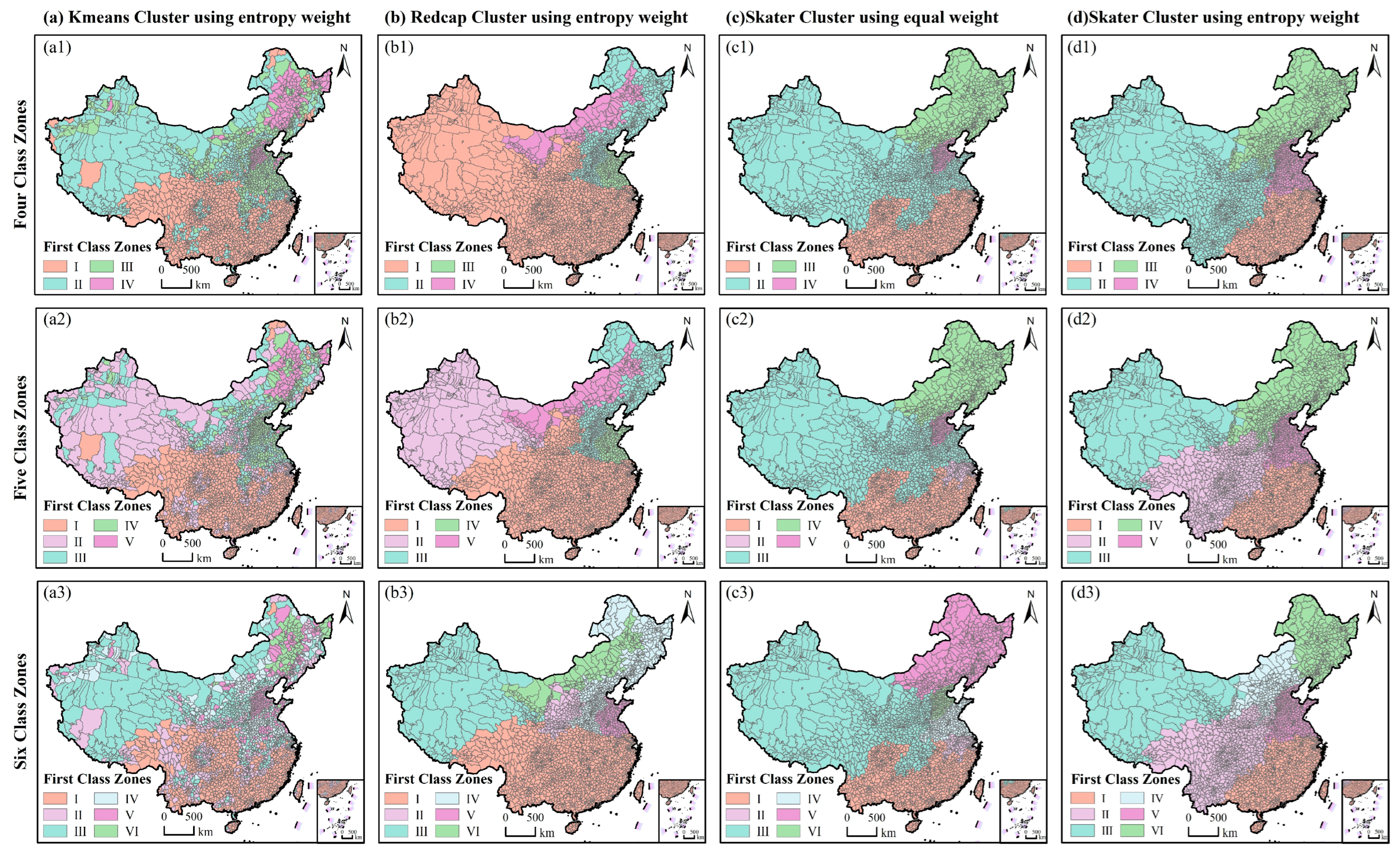
The four clustering approaches exhibit clear differences in their ability to balance attribute separability and spatial structural integrity (Figure 9). The Kruskal–Wallis test indicates that all methods can significantly differentiate the CRCDI among zones (p < 0.05), confirming their basic statistical effectiveness. However, substantial differences are observed in spatial explanatory power and structural stability.

Residual Moran’s I was used to quantify the extent to which each method explains the spatial dependence of CRCDI (

Table 3. Spatial specificity evaluated by residual-based Moran’s I.

Moran Index	Kmeans (Entropy Weight)	Redcap (Entropy Weight)	Skater (Equal Weight)	Skater (Entropy Weight)
Four Class Zones	0.04	0.14	0.19	0.11
Five Class Zones	0.04	0.12	0.14	0.10
Six Class Zones	0.02	0.11	0.12	0.10

). The entropy-weighted Kmeans method, which does not impose spatial constraints, yields the lowest residual Moran’s I values (0.02–0.04), reflecting strong global variance fitting but resulting in highly fragmented and spatially discontinuous zones. In contrast, methods incorporating spatial contiguity constraints show increased residual spatial autocorrelation due to the trade-off between spatial connectivity and attribute homogeneity. Specifically, Redcap (spatially constrained, entropy-weighted) produces residual Moran’s I values ranging from 0.11 to 0.14, while the equal-weight Skater method yields higher values of 0.12–0.19. The proposed entropy-weighted Skater approach achieves consistently lower residual Moran’s I (0.10–0.11) than both Redcap and equal-weight Skater, while maintaining spatial contiguity, indicating a more favorable balance between spatial structure preservation and attribute explanatory power.

Semivariogram analysis further reveals pronounced differences in intra-zone heterogeneity and spatial structural stability (Figure 10). The Kmeans-based zoning (Figure 10(a1–a3)) exhibits a low sill (approximately 12) and a dominant nugget effect, indicating weak spatial continuity and highly fragmented regional structures. The incorporation of spatial constraints in Redcap and Skater substantially improves spatial coherence. However, the proposed entropy-weighted Skater method shows markedly lower residual sill values (approximately 62; Figure 10(d1–d3)) than Redcap (approximately 78; Figure 10(b1–b3)), corresponding to a reduction in within-zone variance of about 20%. Moreover, its semivariograms conform well to a spherical model and reach the sill at a range of approximately 200 km, suggesting that the main spatial structural characteristics are effectively captured while localized noise within zones is suppressed.

These quantitative results demonstrate that the proposed entropy-weighted Skater method achieves an optimal trade-off between attribute homogeneity and spatial contiguity [24,34,35]. By integrating entropy-based indicator weighting with graph-theory-based spatial constraints, the method not only preserves the natural spatial organization of cropland classification difficulty but also enhances within-zone structural coherence, yielding zoning patterns that are more consistent with the intrinsic spatial heterogeneity of agricultural and geographic systems.

5.2.2. Influence of the Zoning Numbers

The selection of the number of zones (k) fundamentally controls the trade-off between the spatial representational detail of cropland remote sensing classification difficulty and the integrity of geographic functional units. By combining the spatial contiguity property of the Skater algorithm with geographical interpretation and statistical evaluation, this study identifies k = 5 as the most appropriate configuration for first-tier cropland zoning.

When the number of zones is small (k = 2–4), the resulting partitions exhibit an evident over-generalization, in which regions characterized by fundamentally different monitoring mechanisms are merged. For example, at k = 4 (Figure 9(d1)), the NAS and QTP regions, dominated by sparse cropland and complex surface backgrounds, are grouped together with the southwestern mountainous regions, where persistent cloud cover and strong topographic fragmentation prevail. From an operational remote sensing perspective, these areas face distinct constraints and require different monitoring strategies, such as mixed-pixel decomposition in low-density cropland regions versus multi-source data fusion and spatiotemporal gap filling in cloud-prone mountainous areas. Merging such mechanism-heterogeneous regions weakens the geographical interpretability of the zoning and reduces its value for guiding region-specific monitoring strategies.

In contrast, an excessive number of zones (k = 6) leads to unnecessary fragmentation of geographically coherent agricultural systems (Figure 9(d3)). Typical examples include the artificial subdivision of the NEP and its transitional areas, which are characterized by highly consistent phenological patterns, cropping systems, and field structures. Such over-partitioning does not reveal meaningful differences in remote sensing monitoring requirements, but instead disrupts the spatial integrity of major agricultural production regions and increases redundancy in practical management.

Therefore, the five-zone scheme represents an optimal compromise. It effectively distinguishes major remote sensing monitoring environments across China, while preserving the integrity of key agricultural regions and ensuring clear geographical meaning. This configuration provides a practical and interpretable spatial framework for large-scale operational cropland classification and regionalized algorithm selection.

Future studies may further extend this framework toward hierarchical, multi-scale zoning to support applications ranging from national-scale strategic assessments to fine-resolution, county-level monitoring.

5.3. Consistency Between the Proposed Zoning Scheme and Existing Zoning Frameworks

The agricultural zoning scheme developed in this study—explicitly oriented toward remote sensing applications—demonstrates superior spatial rationality and geographic adaptability compared with existing frameworks, including the comprehensive agricultural zoning system, the agricultural resource–environment regionalization, and the eco-geographical humidity zoning.

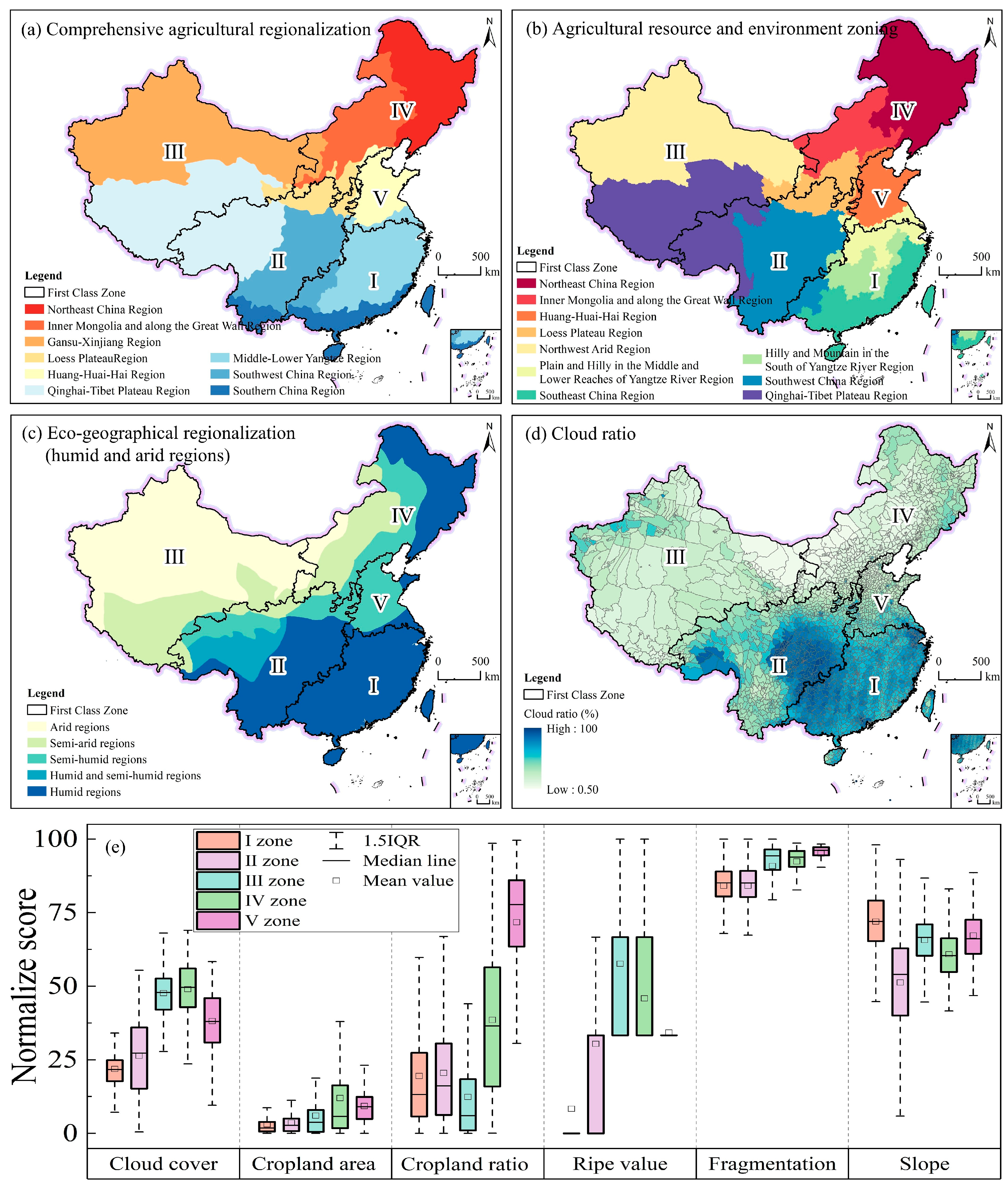
Compared with the comprehensive agricultural regionalization, Zone V and Zone IV identified in this study exhibit a high degree of spatial consistency with the HHH, the NEP, and the Inner Mongolia Great Wall-adjacent region, respectively. This correspondence indicates that in extensive plain regions where agricultural production conditions and remote sensing observation environments are relatively homogeneous, the proposed regionalization demonstrates strong robustness (Figure 11a).

In SC, this study further subdivides the South China region, which is traditionally treated as a single unit in conventional agricultural regionalization, into Zone I and Zone II. This refinement is motivated by practical constraints in remote sensing monitoring. Specifically, Zone II is subject to a weaker influence of maritime water vapor, as indicated by a higher inverse-normalized mean of cloud-cover frequency (inverse-normalized mean = 26.33, SD = 12.08; higher values denote weaker moisture influence), and exhibits significantly lower cloud-cover frequency than Zone I (inverse-normalized mean = 21.87, SD = 10.19) (Figure 11d). As a result, optical remote sensing data availability is substantially higher in Zone II, leading to fundamentally different classification strategies under data-limited conditions. Compared with conventional agricultural regionalization, the proposed scheme provides more direct decision support for the selection of remote sensing classification approaches.

Furthermore, the traditional SC region and the MYP both fall within the subtropical monsoon climate zone and share common characteristics, including frequent cloudy and rainy conditions that constrain optical image acquisition, high degrees of cultivated land fragmentation, and similar cropping systems. Consequently, these areas exhibit highly comparable remote sensing classification difficulty, and in practical classification workflows, they face similar challenges and rely on analogous solutions. Treating them as a single unit is therefore more reasonable from a remote sensing-oriented perspective.

The QTP, which is explicitly divided into southeastern and northwestern subregions in comprehensive agricultural regionalization, is also clearly differentiated in this study. The southeastern QTP, characterized by abundant moisture and complex topography, poses substantial challenges for remote sensing interpretation and is classified as Zone II. In contrast, the northwestern QTP is dominated by arid climatic conditions and relatively simple surface cover, resulting in more favorable monitoring conditions. Its remote sensing classification difficulty is more comparable to that of the arid regions of Gansu and Xinjiang, and these areas are therefore jointly classified as Zone III.

When compared with the agricultural resource–environment regionalization (Figure 11b), which emphasizes resource endowments and functional characteristics and subdivides southeastern China into multiple subregions [36], this study consolidates the MYP, the Jiangnan hilly region, and the southeastern coastal region into Zone I. This integration is primarily based on their shared remote sensing traits, including persistent cloud–rain conditions, a high degree of cropland fragmentation, and the dominance of paddy fields, which produce similar spectral behaviors and interpretative environments for remote sensing. Zone IV merges the NEP, the Inner Mongolia–Great Wall transect, and the northern LP from the resource–environment classification. Although agricultural practices differ across these areas, they share key remote sensing monitoring attributes, including large cropland extent (mean cropland proportion = 12.02, SD = 15.70), moderate cloud cover during the growing season (mean = 49.92, SD = 9.39), and drought-based farming systems, justifying their aggregation into a single classification difficulty zone.

Compared with the eco-geographical humid–arid zoning (Figure 11c), the zoning results derived in this study exhibit a strong spatial coupling with the national humid–arid pattern. Zone I is entirely located within the humid region, corroborating the constraining effects of high atmospheric moisture and frequent cloudy–rainy conditions on remote sensing-based agricultural monitoring [37]. Zone II transitions from humid to semi-arid regions along a southeast-to-northwest gradient, reflecting its traversal across China’s topographic staircases and indicating a progressive improvement in remote sensing monitoring conditions as moisture inputs decrease. Zone III is predominantly situated in arid regions, where clear-sky and low-cloud conditions provide favorable environments for remote sensing observations (mean cloud cover = 47.68, SD = 8.54). The spatial configurations of Zones IV and V are also consistent with the humid–arid differentiation, further demonstrating that climatic humidity—through its control on cloud cover and vegetation dynamics—constitutes a fundamental basis for agricultural remote sensing zoning.

Although Zone IV encompasses a transition from humid to arid areas in the eco-geographical humid–arid classification, which is climatologically consistent with China’s natural conditions, this region is dominated by arid agricultural systems from the perspective of agricultural remote sensing classification difficulty. Specifically, it is characterized by predominantly rain-fed farming, a single cropping system, and extensive cultivated land areas. After incorporating additional agricultural practices and land-use characteristics, this region is therefore more appropriately integrated into a single homogeneous zone in the proposed zoning scheme.

6. Conclusions

Agricultural zoning constitutes a fundamental basis for large-scale remote sensing monitoring and national condition surveys, playing an irreplaceable role in advancing the precision and operationalization of wide-area monitoring. In response to the limitations of existing agricultural zoning schemes in directly supporting operational remote sensing applications, this study integrates multi-source earth observation data with agricultural statistical information, and jointly considers multidimensional spatiotemporal constraints, including image availability, cropping structure, farming systems, and topographic conditions. On this basis, a two-tier agricultural zoning framework oriented toward operational remote sensing applications is established. By simultaneously accounting for attribute homogeneity and spatial continuity, the proposed framework provides a scientific reference for method selection in agricultural remote sensing monitoring.

Within the first-tier zoning framework, an entropy-weighted Skater spatial clustering algorithm is employed to delineate China’s agricultural regions into five major zones, namely the SCYP-HDZ, YGSB-HDZ, ANW-MDZ, NNC-LDZ, and HHH-LDZ. The consistency between the resulting zones and multi-source land use products reaches 0.82, 0.77, 0.79, 0.82, and 0.95, respectively. Comprehensive validation using the Kruskal–Wallis test, residual spatial autocorrelation analysis, and semivariogram diagnostics demonstrates that the proposed zoning approach significantly outperforms traditional Kmeans and other spatial clustering methods in balancing intra-zone homogeneity and inter-zone differentiation, while effectively preserving the integrity of spatial structures.

The second-tier agricultural zoning oriented toward major cereal crops provides a total of 50 crop-specific remote sensing classification difficulty zones, including 13 winter wheat zones, 21 maize zones, and 16 rice zones. Accuracy assessment based on field-surveyed validation samples provides preliminary evidence of an inverse relationship between classification accuracy and the proposed zoning scheme across wheat, maize, and rice regions. In the HHH-LDZ winter wheat zones, the OA values of subzones A, B, and C reach 0.83, 0.84, and 0.85, respectively (with corresponding Kappa coefficients of 0.65, 0.68, and 0.69). In the NNC-LDZ maize zones, the OA values of subzones A, C, and D are 0.73, 0.81, and 0.85, respectively (with corresponding Kappa coefficients of 0.48, 0.62, and 0.70). In the SCYP-HDZ rice zones, the OA values of subzones D, E, and F are 0.76, 0.77, and 0.81, respectively (with corresponding Kappa coefficients of 0.51, 0.54, and 0.61). Crop classification accuracy exhibits a systematic decline with increasing regional classification difficulty, providing inverse empirical validation that the proposed zoning scheme effectively supports decision-making in remote sensing monitoring.

The two-tier zoning framework and derived zoning results proposed in this study provide a structured spatial reference that helps address some limitations of conventional agricultural zoning in guiding remote sensing data acquisition and algorithm adaptation. While the framework demonstrates promising utility for stratified sampling design, region-specific algorithm selection, and accuracy assessment within the sampled regions, its effectiveness at the national scale remains to be further validated due to the limited geographic coverage of second-tier validation samples and potential uncertainties in the underlying land-use products. Future work will focus on expanding cross-region and cross-ecoregion validation samples, incorporating high-resolution satellite data to improve reference data quality, and implementing stratified validation schemes guided by the proposed zoning framework. These steps are expected to strengthen the robustness, transferability, and operational reliability of the framework for large-scale agricultural remote sensing monitoring.

References

1. López-Lozano, R.; Baruth, B. An evaluation framework to build a cost-efficient crop monitoring system. Experiences from the extension of the European crop monitoring system. Agric. Syst. 2019, 168, 231–246. [Google Scholar] [CrossRef] [Scilit]
2. Lu, J.; Li, J.; Fu, H.; Zou, W.; Kang, J.; Yu, H.; Lin, X. Estimation of rice yield using multi-source remote sensing data combined with crop growth model and deep learning algorithm. Agric. For. Meteorol. 2025, 370, 110600. [Google Scholar] [CrossRef] [Scilit]
3. Wu, B.; Tian, F.; Zeng, H.; Zhang, M.; Yan, N.; Qin, X.; Ma, Z. Recent advancements of cloud-based global crop monitoring system (CropWatch). Natl. Remote Sens. Bull. 2025, 29, 1918–1937. [Google Scholar] [CrossRef] [Scilit]
4. Xu, S.; Zhu, X.; Chen, J.; Zhu, X.; Duan, M.; Qiu, B.; Wan, L.; Tan, X.; Xu, Y.N.; Cao, R. A robust index to extract paddy fields in cloudy regions from SAR time series. Remote Sens. Environ. 2023, 285, 113374. [Google Scholar]
5. Liu, T.; Yu, L.; Liu, X.; Peng, D.; Chen, X.; Du, Z.; Tu, Y.; Wu, H.; Zhao, Q. A Global Review of Monitoring Cropland Abandonment Using Remote Sensing: Temporal–Spatial Patterns, Causes, Ecological Effects, and Future Prospects. J. Remote Sens. 2025, 5, 0584. [Google Scholar] [CrossRef] [Scilit]
6. Macdonald, R.B.; Hall, F.G. Global Crop Forecasting. Science 1980, 208, 670–679. [Google Scholar] [CrossRef] [Scilit]
7. Wu, B.; Zhang, M.; Zeng, H.; Tian, F.; Potgieter, A.B.; Qin, X.; Yan, N.; Chang, S.; Zhao, Y.; Dong, Q.; et al. Challenges and opportunities in remote sensing-based crop monitoring: A review. Natl. Sci. Rev. 2022, 10, nwac290. [Google Scholar] [CrossRef] [Scilit]
8. Zhang, H.; Xu, Y.; Lu, Y.; Hasi, E.; Zhang, H.; Zhang, S.; Wang, W. Spatiotemporal variations and driving factors of crop productivity in China from 2001 to 2020. J. Environ. Manag. 2024, 371, 123344. [Google Scholar] [CrossRef] [Scilit]
9. Jiang, Y.; Wang, X.; Huo, M.; Chen, F.; He, X. Changes of cropping structure lead diversity decline in China during 1985–2015. J. Environ. Manag. 2023, 346, 119051. [Google Scholar] [CrossRef] [Scilit]
10. Wang, X.; Hao, J.-Q.; Dai, Z.-Z.; Haider, S.; Chang, S.; Zhu, Z.-Y.; Duan, J.-j.; Ren, G.-X. Spatial-temporal characteristics of cropland distribution and its landscape fragmentation in China. Farming Syst. 2024, 2, 100078. [Google Scholar] [CrossRef] [Scilit]
11. Liu, X.; Wang, Z.; Yang, X.; Cheng, W.; Zhang, J.; Liu, Y.; Liu, B.; Meng, D.; Zeng, X. Remotely-sensed phenology pattern regionalization for land cover classification of natural scenes: A case study in China. Acta Geogr. Sin. 2024, 79, 2206–2229. [Google Scholar] [CrossRef]
12. Wang, Z.; Yang, X.; Zhang, J.; Liu, X.; Li, L.; Dong, W.; He, W. A Remote Sensing Intelligent Interpretation Framework Through Geo-Science Zoning for Complex Nature Scenes and Its Preliminary Experiments. J. Geo-Inf. Sci. 2025, 27, 305–330. [Google Scholar] [CrossRef]
13. Lan, X.; Wang, J.; Liu, H.; Liu, X.; Guo, H. Research on zonal protection of cultivated land quality in agricultural counties based on spatial heterogeneity. J. Agric. Resour. Environ. 2025, 42, 844–854. [Google Scholar] [CrossRef]
14. Liao, Y.; Xie, E.; Chen, W.; Yao, D.; Lei, M.; Dang, Y.; Li, L.; Zhao, J.; Kong, X. Comprehensive zoning of cultivated land quality improvement based on synergistic production characteristics and ecological stress in China. Trans. Chin. Soc. Agric. Eng. 2025, 41, 208–217. [Google Scholar] [CrossRef]
15. Xie, Y.; Nhu, A.N.; Song, X.-P.; Jia, X.; Skakun, S.; Li, H.; Wang, Z. Accounting for spatial variability with geo-aware random forest: A case study for US major crop mapping. Remote Sens. Environ. 2025, 319, 114585. [Google Scholar] [CrossRef] [Scilit]
16. Sun, H.; Huang, J.; Li, B.; Wang, H. Study on the Regionalization of Paddy Rice Information Acquirement Through Remote Sensing Technology in China. Sci. Agric. Sin. 2008, 41, 4039–4047. [Google Scholar] [CrossRef]
17. Liu, Y.; Chen, X.; Chen, J.; Zang, Y.; Wang, J.; Lu, M.; Sun, L.; Dong, Q.; Qiu, B.; Zhu, X. Long-term (2013–2022) mapping of winter wheat in the North China Plain using Landsat data: Classification with optimal zoning strategy. Big Earth Data 2024, 8, 494–521. [Google Scholar] [CrossRef] [Scilit]
18. Wang, Y.; Yuan, Y.; Yuan, F.; Liu, X.; Tian, Y.; Zhu, Y.; Cao, W.; Cao, Q. Optimizing management zone delineation through advanced dimensionality reduction models and clustering algorithms. Precis. Agric. 2025, 26, 68. [Google Scholar] [CrossRef] [Scilit]
19. Wang, Y.; Yu, H.; Lu, L. Spatio-temporal pattern and functional zoning of ecosystem services in the Yangtze River Delta region based on spatially constrained K-means. Acta Ecol. Sin. 2024, 44, 7087–7104. [Google Scholar] [CrossRef]
20. Li, X.; Luo, M.; Zhao, Y.; Zhang, H.; Ge, E.; Huang, Z.; Wu, S.; Wang, P.; Wang, X.; Tang, Y. A daily high-resolution (1 km) human thermal index collection over the North China Plain from 2003 to 2020. Sci. Data 2023, 10, 634. [Google Scholar] [CrossRef] [Scilit]
21. Meng, F.; Chen, H.; Tan, Y.; Xiong, W. Changes in crop mix and the effects on agricultural carbon emissions in China. Int. J. Agric. Sustain. 2024, 22, 2335141. [Google Scholar] [CrossRef] [Scilit]
22. Qiu, B.; Hu, X.; Chen, C.; Tang, Z.; Yang, P.; Zhu, X.; Yan, C.; Jian, Z. Maps of cropping patterns in China during 2015–2021. Sci. Data 2022, 9, 479. [Google Scholar] [CrossRef] [Scilit]
23. AssunÇão, R.M.; Neves, M.C.; Câmara, G.; Da Costa Freitas, C. Efficient regionalization techniques for socio-economic geographical units using minimum spanning trees. Int. J. Geogr. Inf. Sci. 2006, 20, 797–811. [Google Scholar] [CrossRef] [Scilit]
24. Aydin, O.; Janikas, M.V.; Assunção, R.M.; Lee, T.-H. A quantitative comparison of regionalization methods. Int. J. Geogr. Inf. Sci. 2021, 35, 2287–2315. [Google Scholar] [CrossRef] [Scilit]
25. Lage, J.P.; Assunção, R.M.; Reis, E.A. A Minimal Spanning Tree Algorithm Applied to Spatial Cluster Analysis. Electron. Notes Discret. Math. 2001, 7, 162–165. [Google Scholar] [CrossRef] [Scilit]
26. Amoroso, N.; Cilli, R.; Nitti, D.O.; Nutricato, R.; Iban, M.C.; Maggipinto, T.; Tangaro, S.; Monaco, A.; Bellotti, R. PSI Spatially Constrained Clustering: The Sibari and Metaponto Coastal Plains. Remote Sens. 2023, 15, 2560. [Google Scholar] [CrossRef] [Scilit]
27. Huang, C.; You, S.; Liu, A.; Li, P.; Zhang, J.; Deng, J. High-Resolution National-Scale Mapping of Paddy Rice Based on Sentinel-1/2 Data. Remote Sens. 2023, 15, 4055. [Google Scholar] [CrossRef] [Scilit]
28. Tang, K.; Chen, X.; Liu, T.; Li, A.; Tang, Y.; Yang, P.; Chen, J. AnytimeFormer: Fusing irregular and asynchronous SAR-optical time series to reconstruct reflectance at any given time. Remote Sens. Environ. 2026, 333, 115120. [Google Scholar] [CrossRef] [Scilit]
29. Li, C.; Lei, L.; Jia, X.; Xiong, X.; Zhang, X. Accuracy and applicability assessment of vegetation types of the land cover products produced in China. Ecol. Indic. 2025, 174, 113506. [Google Scholar] [CrossRef] [Scilit]
30. Li, P.; Wang, Y.; Wang, C.; Tian, L.; Lin, M.; Xu, S.; Zhu, C. A Comparison of Recent Global Time-Series Land Cover Products. Remote Sens. 2025, 17, 1417. [Google Scholar] [CrossRef] [Scilit]
31. Xue, J.; Zhang, X.; Chen, S.; Hu, B.; Wang, N.; Shi, Z. Quantifying the agreement and accuracy characteristics of four satellite-based LULC products for cropland classification in China. J. Integr. Agric. 2024, 23, 283–297. [Google Scholar] [CrossRef] [Scilit]
32. Shi, P.; Wang, J.; Zhang, G.; Kong, F.; Wang, J. Research review and prospects of natural disasters regionalization in China. Geogr. Res. 2017, 36, 1401–1414. [Google Scholar]
33. Zhu, Q.; Ran, L.; Zhang, Y.; Guan, Q. Integrating geographic knowledge into deep learning for spatiotemporal local climate zone mapping derived thermal environment exploration across Chinese climate zones. ISPRS J. Photogramm. Remote Sens. 2024, 217, 53–75. [Google Scholar] [CrossRef] [Scilit]
34. Hao, G.; Lei, D.; Lun, W.; Yu, L. Tackling spatial heterogeneity in geographical analysis: An overview. Acta Geogr. Sin. 2025, 80, 567–585. [Google Scholar] [CrossRef]
35. Kim, N.; Yoon, Y. Regionalization for urban air mobility application with analyses of 3D urban space and geodemography in San Francisco and New York. Procedia Comput. Sci. 2021, 184, 388–395. [Google Scholar] [CrossRef] [Scilit]
36. Xu, E. Dataset of Agricultural Resource and Environment Zoning of China. J. Glob. Change Data Discov. 2021, 5, 19–26. [Google Scholar] [CrossRef] [Scilit]
37. Wang, F.; Li, B.; Tian, S.; Zheng, D.; Ge, Q. Updated scheme for eco-geographical regionalization in China. Acta Geogr. Sin. 2024, 79, 3–16. [Google Scholar] [CrossRef]
Figure 1. The map of nine agricultural zones in China with a backdrop of DEM and crop maps. The DEM were obtained from the Resource and Environment Data Cloud Platform (http://www.resdc.cn/, accessed on 1 May 2025) supported by the Institute of Geographic Sciences and Natural Resource and the crop maps were derived from the National Ecosystem Science Data Center (https://nesdc.org.cn/, accessed on 1 May 2025).
Remotesensing 18 00831 g001
Figure 2. Overall technical framework.
Remotesensing 18 00831 g002
Figure 3. The CRCDI based on the entropy-weight method and the first-tier zoning indicators.
Remotesensing 18 00831 g003
Figure 4. First-tier cropland zoning results and the trend of cluster variation. (ae) represent the results of the number of zones for categories 2–6; (f) represents the trend of the number of zones and the evaluation indicators of the zones; and (g) represents the classification difficulty index of each zone under the optimal number of zones.
Remotesensing 18 00831 g004
Figure 5. Validation of cropland reliability and uncertainty in the first-tier agricultural zoning.
Remotesensing 18 00831 g005
Figure 6. Cropland and major cereal crop area proportions within the first-tier agricultural zones.
Remotesensing 18 00831 g006
Figure 7. Second-tier agricultural zoning for major cereal crops. (ac) Spatial distribution of the second-tier zoning results for wheat, maize, and rice, respectively. (d) The corresponding number of second-tier subzones.
Remotesensing 18 00831 g007
Figure 8. Validation of the second-tier agricultural zoning for major cereal crops. (a,b) Spatial distribution of sample points and the validation accuracy for wheat in Zone V; (c,d) Spatial distribution of sample points and the validation accuracy for maize in Zone IV; and (e,f) Spatial distribution of sample points and the validation accuracy for rice in Zone I.
Remotesensing 18 00831 g008
Figure 9. Comparison across clustering methods and zoning numbers. (a1a3) represent the results of the number of zones of 4–6 categories calculated using the entropy-weighted Kmeans Cluster method, respectively; (b1b3) represent the results of the number of zones of 4–6 categories calculated using the entropy-weighted Redcap Cluster method, respectively; (c1c3) represent the results of the number of zones of 4–6 categories calculated using the equal-weighted Skater Cluster method, respectively; and (d1d3) represent the results of the number of zones of 4–6 categories calculated using the entropy-weighted Skater Cluster method, respectively.
Remotesensing 18 00831 g009
Figure 10. Semivariogram modeling based on residuals. (a1a3) represent the semivariogram results of 4 to 6 categories calculated using the entropy-weighted Kmeans Cluster method, respectively; (b1b3) represent the semivariogram results of 4 to 6 categories calculated using the entropy-weighted Redcap Cluster method, respectively; (c1c3) represent the semivariogram results of 4 to 6 categories calculated using the equal-weighted Skater Cluster method, respectively; (d1d3) represent the semivariogram results of 4 to 6 categories calculated using the entropy -weighted Skater Cluster method, respectively.
Remotesensing 18 00831 g010
Figure 11. Comparison across zoning schemes and normalized scores of indicators within the first-tier zones. (a) represents the comparison between the first- tier zones and the comprehensive agricultural regionalization; (b) represents the comparison between the first-tier zones and the agricultural resource and environment zoning; (c) represents the comparison between the first-tier zones and the eco-geographical regionalization; (d) represents the comparison between the first-tier zones and the cloud coverage frequency; and (e) represents the normalized scores of each constituent indicator within the first-tier zones.
Remotesensing 18 00831 g011