Siamese-ViT: A Local–Global Feature Fusion Method for Real-Time Visual Navigation of UAVs in Real-World Environments

Highlights

What are the main findings?

• We propose a Siamese-ViT-based aerial image–satellite image mapping architecture for real-time visual navigation. The backbone network uses ViT as the global feature extractor and implements a weight-sharing mechanism to improve the model’s ability to handle cross-view geolocation. We employ a K-means-based local feature aggregation method to address the efficiency and matching complexity issues caused by high-dimensional features in visual scene matching tasks. This method aggregates local features into a fixed number of cluster centers, compressing high-dimensional features and effectively improving retrieval efficiency.
• To improve the real-time performance of matching, we use IPCA to reduce the dimensionality of the feature space. Furthermore, we construct a KD-tree structure from the feature vector library of satellite images, recursively transforming the high-dimensional space into a series of hyperrectangular regions for efficient searching.

What are the implications of the main findings?

• To address the navigation challenges in complex terrain environments under satellite denial, our method integrates local fine-grained information with global semantic information and uses IPCA to reduce the dimensionality of the feature space, providing a feasible solution for autonomous flight of UAVs.
• To address the challenge of real-time visual navigation in real-world scenarios, we collected aerial photography data from various complex real-world environments to validate our algorithms, laying the foundation for the application of deep learning in intelligent positioning.

Abstract

Visual scene matching navigation (VSMN) for unmanned aerial vehicles (UAVs) boasts advantages such as high precision, high reliability, and autonomy. The biggest challenge lies in the tension between local fine-grained information and global semantics, as well as limited generalization ability in real-world environments. While existing Transformer-based cross-view geolocation methods enhance global context modeling capabilities, they still generally face issues such as high demands on training data and computational resources, insufficient fusion of local fine-grained information and global semantics, and real-time performance in real-world complex environment. To address these problems, we propose a scene matching and localization algorithm based on the Siamese-ViT. For feature extraction, we use the ViT model to extract global features and K-means clustering to aggregate local features. Combined with the global features extracted by the ViT, a robust local–global feature representation vector is generated. For feature matching, incremental principal component analysis (IPCA) is used to reduce the dimensionality of the high-dimensional feature space, and a KD-tree is constructed for fast feature retrieval to improve matching efficiency. We validated our algorithm on the University-1652 dataset and a dataset of real-world satellite-drone image pairs. The results show that our Siamese-ViT outperforms other models in both Recall and AP. We conduct flight experiments in real-world environments, capturing drone images of complex scenes, including farmland, urban buildings, and waterways. The results show that, at a flight altitude of 350 m, our algorithm achieves an average absolute value of 6.2063 m for latitude, 6.7552 m for longitude, and 10.1922 m for horizontal error. Therefore, our Siamese-ViT demonstrates ideal overall positioning accuracy.

1. Introduction

UAVs are widely used in remote sensing applications, such as environmental monitoring and disaster response. Reliable navigation is a fundamental requirement for autonomous UAV flight. While Global Navigation Satellite Systems (GNSS) can provide accurate positioning in open skies, their performance degrades significantly in complex environments due to factors such as signal congestion, multipath effects, and human interference. These limitations have prompted the development of alternative navigation methods that remain robust even when GNSS signals are limited or weakened.

VSMN is a core technology in UAV autonomous positioning. By matching real-time visual information acquired by image sensors with reference satellite images, VSMN can achieve high-precision absolute position estimation and path planning in large-scale environments. Especially in environments with weak or unavailable GPS signals, VSMN has become a highly promising UAV navigation solution.

However, existing VSMN methods still face several challenges. Firstly, sensor position, shooting angle, and environment changes make the cross-view matching performance decrease. Secondly, dynamic changes, lighting conditions, and occlusion in real-world environments make visual matching even more difficult. Furthermore, while existing deep learning methods perform well on training sets, dependence on data and the scarcity of labeled samples often lead to insufficient generalization in practical applications.

Early VSMN methods for UAVs primarily relied on manual feature extraction and geometric matching techniques. Lowe D G proposed SIFT [1], which is invariant to rotation and scale changes, but inaccurate matching can still occur under strong lighting variations or dynamic lighting conditions. Bay H [2] improved the speed of feature extraction and matching by using approximate calculations of the Hessian matrix. E Rublee [3] combined FAST corner detection and BRIEF descriptors, making it suitable for real-time applications, especially in resource-constrained environments. V Lepetit [4] utilized 3D models and 2D feature points extracted from images to perform accurate pose estimation using geometric relationships. PJ Besl [5] estimated pose by matching point clouds of source and target images through iterative optimization. Mark Cummins et al. [6] modeled location recognition as a large-scale appearance-only SLAM problem and achieved large-scale scene retrieval by learning the co-occurrence probability of visual words. Milford M. et al. [7] further proposed a sequence-based matching strategy rather than a single frame, which significantly improved robustness under conditions of drastic changes in day and night, seasons and weather, indicating that temporal consistency plays an important role in location revisit identification in navigation scenarios. Wang Z. [8] transformed the large-scale 2D image matching task into sequence matching based on UAV trajectory, and effectively improved the accuracy and robustness of geographic positioning by combining sorting and matching with depth and classical methods. Baykal F. [9] provided a comprehensive UAV image matching evaluation framework, which provides clear experimental support for the advantages and disadvantages of traditional and depth methods, especially in scenes with significant differences in high altitude and resolution. Therefore, while early UAV visual scene matching navigation methods can provide a certain level of accuracy and robustness in specific environments, they generally suffer from drawbacks such as high computational cost, sensitivity to changes in illumination and scale, and high environmental requirements.

Advances in deep learning have significantly improved the performance of visual scene matching. Early deep learning-based UAV visual scene matching navigation methods mainly followed the retrieval paradigm of Siamese networks or convolutional neural networks (CNNs), aiming to learn a shared embedding space for cross-view image matching. Sixing Hu et al. [10] used Siamese networks combined with NetVLAD aggregation to learn robust global descriptors for cross-view geolocation, while Yujiao Shi et al. [11] further improved matching performance by introducing spatially aware feature aggregation and coarse geometric alignment between different viewpoints. With the release of the University-1652 [12] dataset, UAV-based target localization and UAV navigation can now be performed under a unified benchmark. T Wang et al. [13] shifted from purely global representation learning to local perceptual modeling, utilizing square ring local partitioning to capture contextual cues centered on the target and its neighboring regions, thereby improving cross-view discrimination under changing perspectives. Arandjelović et al. [14] proposed NetVLAD, which integrates a differentiable VLAD aggregation layer into a CNN, achieving end-to-end global representation learning for large-scale visual location recognition. Noh et al. [15] proposed a scene matching method based on CNN. Hausler S et al. [16] further introduced multi-scale patch-level local matching in addition to global description to balance fast retrieval and fine-grained verification, promoting the development of the coarse retrieval-fine matching two-stage paradigm. Recent research has focused more on training scalability, view robustness, and description efficiency. Berton G et al. [17] proposed a more scalable training strategy for large-scale visual geolocation at the city level and verified the limitations of existing methods in real urban scenes on a larger dataset. Ali-bey A et al. [18] replaced complex local or pyramid aggregation with cascaded feature blending, significantly reducing parameter count and inference burden while maintaining high recall. Liao et al. [19] proposed an Adaptive Threshold Guided Ring Partitioning Framework, which effectively mitigates the domain differences between UAV and satellite images by combining CNN feature extraction, adaptive spatial partitioning, and brightness alignment preprocessing, thereby achieving more accurate geolocation results. Li M. [20] proposed a deep learning framework integrating geographic information, built a twin network of two branches to extract features from satellite UAV cross-view remote sensing images, and embedded geospatial constraints into model training. In recent years, semantic-based methods have also been explored to mitigate appearance differences. Tian Y. et al. [21] designed a single-stream pyramid Transformer network (SSPT), which uses a self-attention mechanism to enrich its internal features and a cross-attention mechanism to refine and interact with different features in order to eliminate irrelevant interference. Tian X. et al. [22] integrated a cross-view synthesis module and a geolocation module, fully considering the spatial correspondence between the UAV view and the satellite view, as well as the surrounding area information. Zhang X. et al. [23] combined the semantic understanding capabilities of Vision Language Models (VLM) with traditional visual feature matching to propose a cross-view localization architecture that is more in line with real-world localization scenarios, which can improve accuracy in small field-of-view image matching. Zhang H. et al. [24] used Patch Aware Feature Aggregation (PAFA) to emphasize closer mutual information interaction between local patches, improving the consistency and matching ability of features across different perspectives. Y. Ji [25] proposed MMGeo which performs cross-view UAV geolocalization merely with a single satellite base map, which effectively eliminates the dependency on heavy offline dataset construction and better adapts to real-world low-altitude flight scenarios. The significance of these methods lies in their expansion of traditional “same-view revisit recognition” into “different-view semantic alignment and location retrieval,” enabling visual scene matching navigation to break free from its reliance on high-density ground databases and instead achieve positioning using broader aerial or satellite imagery.

In recent years, an increasing number of studies have adopted Transformer-based architectures and adaptive matching strategies to address the severe perspective differences, positional shifts, and scale uncertainties between UAV and satellite imaging [26]. FSRA [27] introduced heatmap-guided feature segmentation and region alignment, enabling more flexible local correspondence modeling without relying on manually predefined region partitioning. Yang H. et al. [28] pointed out that this task not only requires understanding the semantic content of images, but also establishing spatial layout correspondences between different perspectives, and therefore proposes layer-to-layer Transformers for cross-layer association modeling. TransGeo [29] demonstrated that pure Transformer models can achieve robust cross-view geolocalization performance by utilizing attention-guided non-uniform cropping and global context modeling. Sample4Geo [30] showed that a simplified contrastive framework combined with hard negative sampling can achieve competitive or even superior results, highlighting the importance of training strategies beyond network design. In general, current research has progressed from global descriptor learning to adaptive region modeling, Transformer-based representation learning, and more generalized optimization strategies. To improve computational efficiency, Liu et al. [31] proposed the Swin Transformer, which adopts a window-based hierarchical attention mechanism and has been applied in the fields of UAVs and remote sensing. S. S. Kannan et al. [32] selected image patches of different scales to extract multi-level features in the image and introduced a dynamic patch selection mechanism to improve the efficiency and accuracy of the model, which has strong robustness in complex and dynamic environments. Tian Z. et al. [33] proposed to integrate semantic information (such as object category, scene label, etc.) into visual features, so that the model can understand and locate the scene more accurately. O Grainge et al. [34] proposed a ternary-quantized Transformer for visual location recognition and scene matching, with particular attention on the balance between computational efficiency and performance in embedded and low-resource environments. Zhang, F. et al. [35] introduced a sparse expert mechanism inside the encoder, which adaptively activates different experts based on the content, scale, and source of each grid, thereby improving the ability to learn cross-viewpoint and cross-scale dependent features. However, maintaining robustness in complex real-world UAV navigation scenarios remains an unresolved challenge.

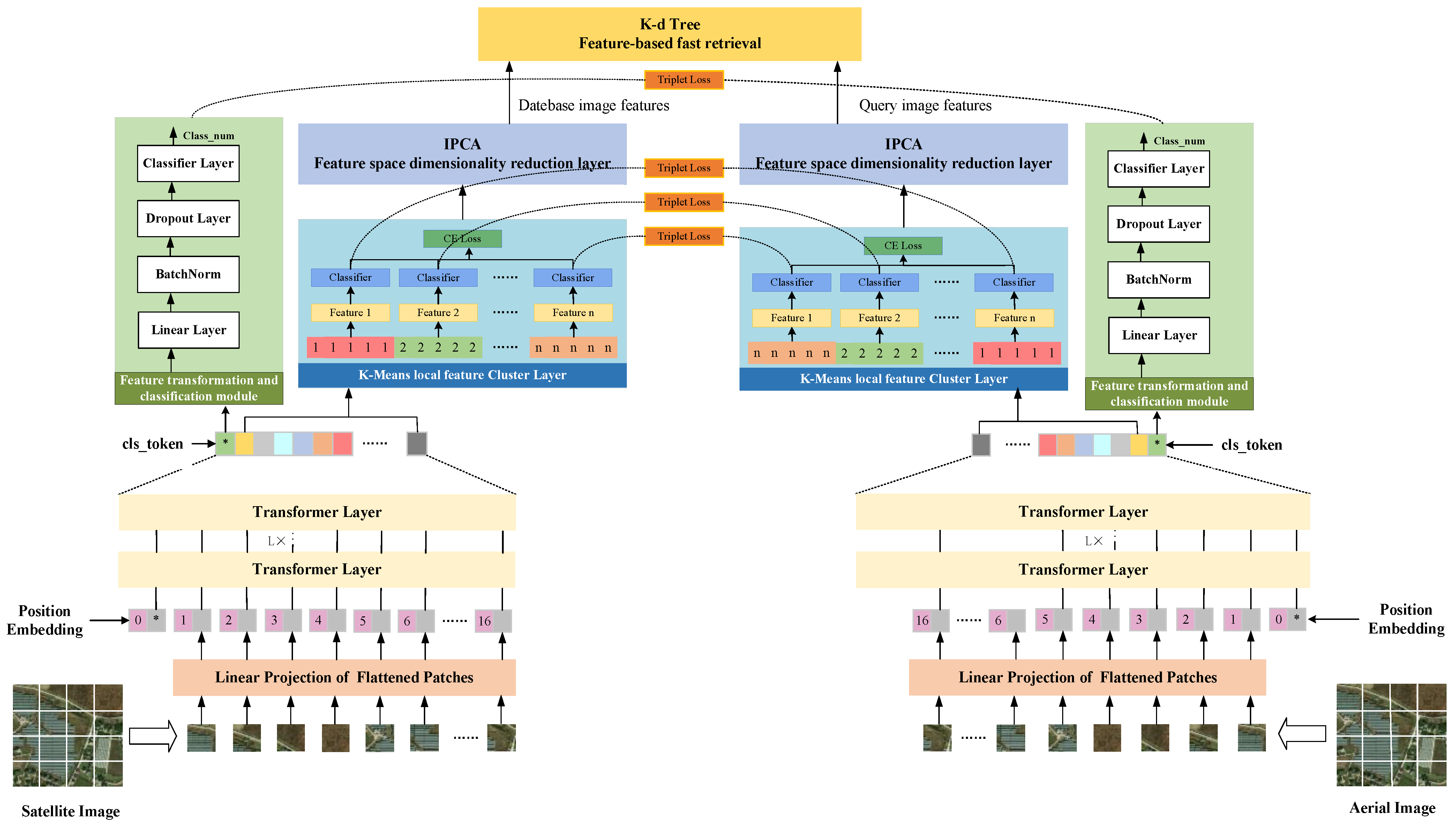
To improve the model’s ability to handle cross-view geolocation, we employ a Siamese neural network framework to map aerial images and reference satellite images to the same feature space. The backbone network uses ViT as the model’s global feature extractor. The input consists of satellite and aerial images of the same size, and the backbone network shares weights. Compared to traditional methods, our approach retains the inherent advantages of Siamese networks in pairwise similarity learning and retrieval-based localization, while leveraging ViT’s self-attention mechanism to enhance cross-regional context modeling capabilities.

To strengthen the fusion of global semantic features and local fine-grained information, we use ViT as the global feature extraction framework. Simultaneously, we employ a K-means-based local feature aggregation method, aggregating local features into a fixed number of cluster centers to compress high-dimensional features, improve retrieval efficiency and matching complexity, and reduce the impact of noise on matching.

Real-time performance is a major challenge in current UAV visual navigation. Our model trains to make the feature vectors of aerial and satellite images similar, but the distribution of their feature spaces still differs. To optimize the feature space and improve the efficiency of the feature matching algorithm, we employ incremental principal component analysis (IPCA) to reduce the dimensionality of the feature space, effectively improving matching efficiency and reducing computational burden. To further enhance feature matching efficiency and quickly obtain initial retrieval results, we construct a KD-tree structure from the feature vector database of satellite images. We divide its subspace into left and right subtrees, recursively transforming the high-dimensional space into a series of hyperrectangular regions for efficient searching.

In summary, our contributions are as follows:

• We propose an aerial image–satellite image mapping architecture based on Siamese-ViT. The backbone network uses ViT as the global feature extractor and implements a weight-sharing mechanism to improve the model’s ability to handle cross-view geolocation.
• To address the issues of retrieval efficiency and matching complexity caused by high-dimensional features in visual scene matching tasks, we employ a K-means local feature aggregation method on top of the ViT global feature extraction framework. This method aggregates local features into a fixed number of cluster centers, compressing high-dimensional features and effectively improving retrieval efficiency.
• To improve the real-time performance of matching, we use IPCA to reduce the dimensionality of the feature space. Furthermore, we construct a KD-tree structure from the feature vector library of satellite images, recursively transforming the high-dimensional space into a series of hyperrectangular regions for efficient searching.

2. Methods

This section introduces a scene matching localization method and model architecture based on Siamese-ViT, where, given a set of satellite images and aerial images, the goal is to effectively establish accurate correspondences between image pairs to achieve precise scene matching localization.

2.1. Global Feature Extraction Based on ViT

To better adapt to the scene matching task during training, we constructed a strong baseline for scene matching localization based on ViT, the structure of which is shown in Figure 1. The two inputs are satellite images and aerial images of the same size. We selected the ViT model as the feature extraction branch and constructed two ViT models with equal weights into a Siamese neural network architecture.

For a given input image, $x\in {\mathbb{R}}^{H\times W\times C}$, which is divided into N fixed-size patches with the size of P × P × C. In ViT, all patches are projected onto a fixed vector space, forming a unified patch embedding dimension. Simultaneously, an additional learnable location embedding $x_{cls}$ is incorporated into its location space, and robust global feature vectors are extracted through supervised learning. The input sequence is shown in Equation (1):

$$Z_0=\left[x_{cls};F\left(x_p^1\right);F\left(x_p^2\right);\cdots ;F\left(x_p^N\right)\right]+P$$

(1)

where $F$ represents the linear projection of the patch onto a D-dimensional vector, and $P\in {\mathbb{R}}^{\left(N+1\right)\times D}$ represents the position encoding matrix with the same dimension as the patch embedding, and the parameters are learnable.

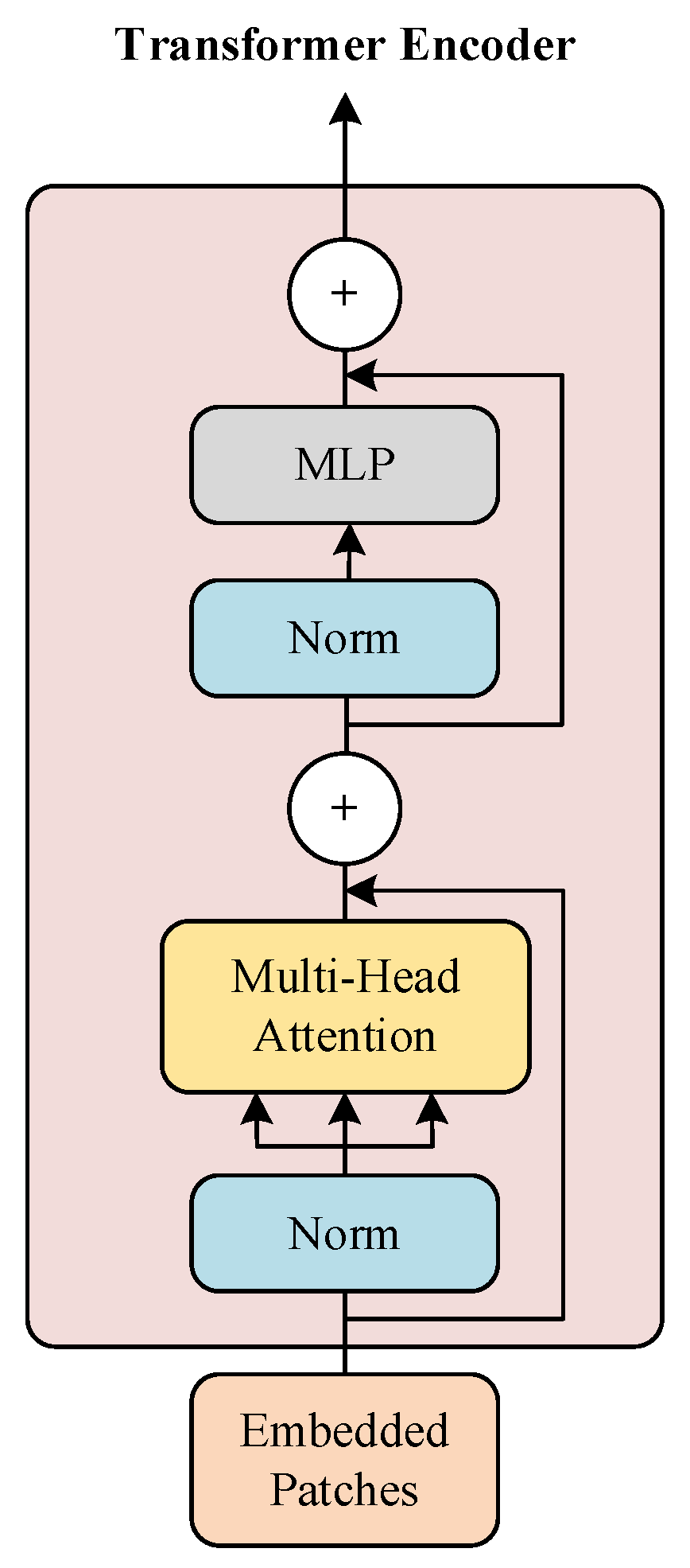
The input sequence is processed through repeated stacked Encoder Blocks for feature extraction, as shown in Figure 2. The input consists of patches containing position embeddings. The Encoder Block comprises four components: layer normalization, multi-head attention, another layer normalization, and an MLP layer. After iterative processing via multi-head attention and a feedforward network, each embedded patch includes a class token, which interacts with each other through a self-attention mechanism. This means that the class token, as part of the Query, Key, and Value, undergoes attention calculation with all patch tokens, gradually aggregating information from the entire image. Furthermore, the class token is fixed at the beginning of the sequence (position 0), and its initialization is independent of specific image content. This design avoids bias towards a particular patch, focusing more on the summarization of global semantics rather than local details. L× represents the Encoder Block being repeated L times.

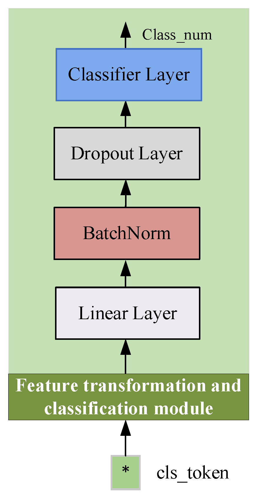
Finally, we perform global feature transformation and classification operations on the class token, as shown in Figure 3. This part includes a Linear layer, Batch normalization, and Dropout layer. The linear layer mainly performs dimensionality transformation, outputting global features of the specified dimensions. Finally, a classifier transforms the dimensions into the number of classes.

2.2. Local Feature Aggregation Based on K-Means

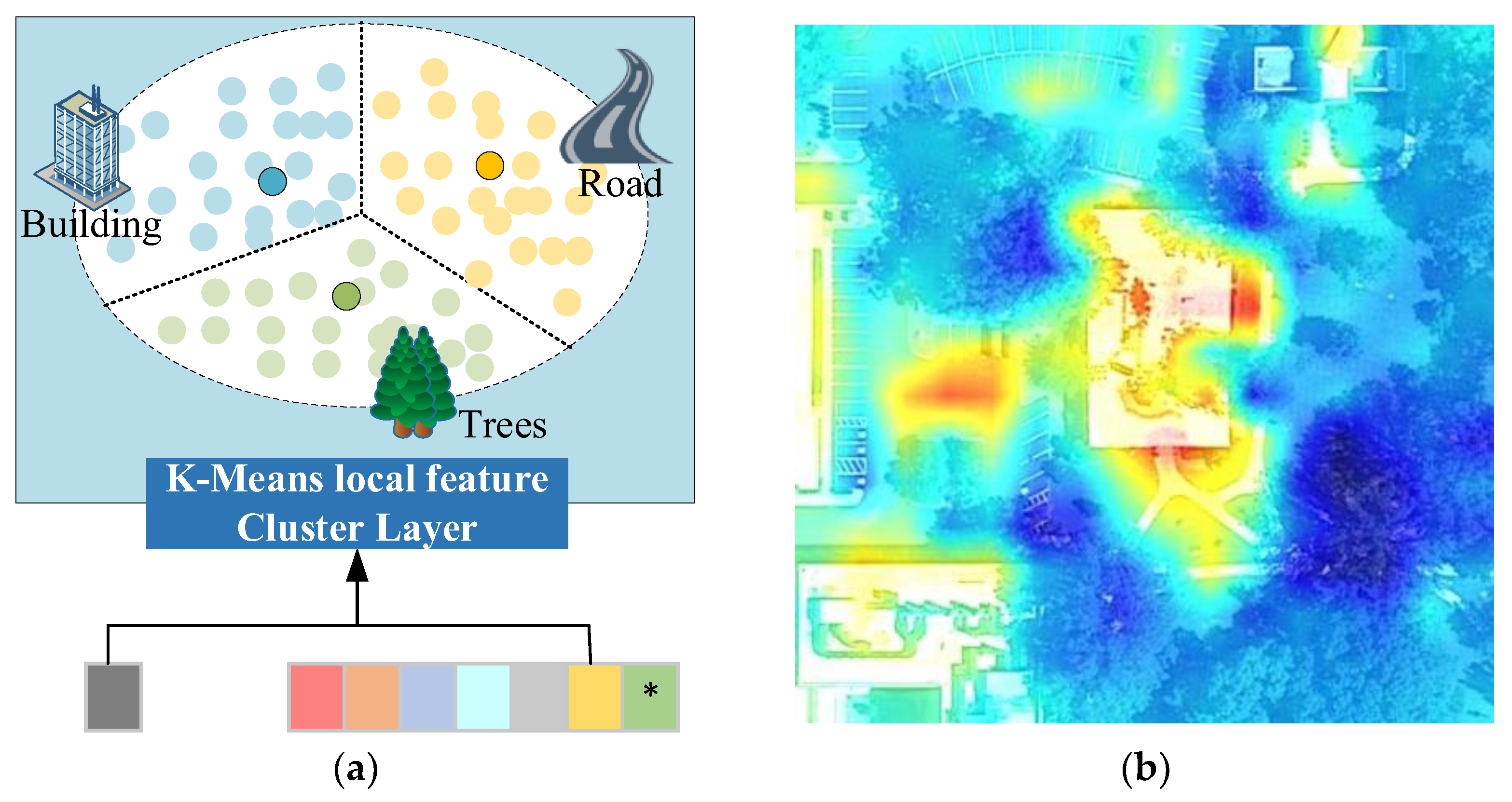
After feature extraction based on ViT, 256-dimensional local features are formed. Image matching often requires real-time performance, and direct feature matching would incur significant computational and storage costs. Furthermore, local features may contain noise points. Therefore, clustering local features is meaningful. We analyzed a large number of aerial images and found that the main semantic feature categories are buildings, roads, and trees. Therefore, we used K-means to cluster local features into a fixed number of “cluster centers,” compressing high-dimensional features, improving retrieval efficiency and matching complexity, and reducing the impact of noise on matching, as shown in Figure 4a.

For the patch tokens extracted by the ViT model above, three learnable cluster centers ${\mu }_i$ are first randomly initialized, and for each patch token, the distance to the three cluster centers is calculated, as shown in Equation (2):

$$d\left(x,{\mu }_i\right)={\sum }_{x\in c}{‖x-{\mu }_i‖}^2$$

(2)

where c represents the set of patch tokens, $x$ is a feature vector belonging to c, Euclidean distance is used to measure the distance of the feature vector to the cluster center, and n is the number of categories, which we take as 3. Our goal is to minimize the sum of squared errors within a cluster; that is, to minimize the sum of squared distances from each feature vector to its respective cluster center, as shown in Equation (3):

$$J={\sum }_{i=1}^{n}d\left(x,{\mu }_i\right)$$

(3)

We employ a soft allocation method instead of the traditional hard allocation method. We calculate cluster centers using a weighted average and update the membership matrix based on the distance between each data point and a cluster center. We obtain the allocation weights for each feature vector by calculating the probability of it being assigned to one of the three cluster centers, as shown in Equation (4):

$$q_i={\displaystyle \frac{{\left(1+\frac{{‖x-{\mu }_i‖}^2}{\alpha }\right)}^{-\frac{\alpha +1}{2}}}{{\sum }_{i^{\prime }}{\left(1+\frac{{‖x-{\mu }_{i^{\prime }}‖}^2}{\alpha }\right)}^{-\frac{\alpha +1}{2}}}},i=\mathrm{1,2},3$$

(4)

where $\alpha$ represents the hyperparameter used to control the degree of soft assignment, and $q_i$ represents the probability that the feature vector belongs to each cluster center. The feature-weighted average of each cluster center is given by Equation (5):

$$y_i=q_i^{T}x,i=\mathrm{1,2},3$$

(5)

After normalization, the local features of the three categories are obtained and input into the classifier for feature transformation and classification. The classifier structure is similar to that of the global feature classifier. Finally, the cluster features of the (512, 3) dimensions and their classification probabilities are the output, which are used to calculate the cross-entropy loss and triplet loss so as to update the cluster centers during backpropagation. After local feature aggregation, the spatial distribution of the image can be well represented, as shown in Figure 4b. Overlaying the features extracted by the model with the original image clearly separates features such as buildings, roads, and trees, demonstrating excellent feature extraction capabilities.

2.3. Feature Space Dimensionality Reduction Based on IPCA

The model trains aerial and satellite image feature vectors to be similar, but the distribution of their feature spaces still differs. To optimize the feature space and improve the efficiency of the feature matching algorithm, this paper employs incremental principal component analysis (IPCA) to reduce the dimensionality of the feature space. IPCA can progressively update principal components when processing new data without recalculating the covariance matrix of the entire dataset, making it particularly suitable for large-scale datasets and online data stream scenarios.

Assume the satellite image data $X$ is a 3D vector $X={\left(X_1,X_2,\cdots ,X_n\right)}^T,X_i\in R^D$. Assume the current batch of data being processed is $X^t$, and the total number of data points is t. Calculate the batch mean $u^t$ and the batch covariance matrix $C^t$.

$$u^t={\displaystyle \frac{1}{t}}{\sum }_{i=1}^t{X}_i$$

(6)

$$C^t={\displaystyle \frac{1}{t}}{\displaystyle {\sum }_{i=0}^t}(X_i-u^{\left(t\right)}){(X_i-u^{\left(t\right)})}^T$$

(7)

Perform SVD decomposition on $C^t$ to obtain eigenvectors $V$ and eigenvalues $\Lambda$.

$$C^t=V\Lambda V^T$$

(8)

The first k principal components are selected to form a new projection matrix $W_k$. This process is performed on all batches of data, using the updated principal component matrix $W_k$ to reduce the dimensionality of the new data. $W_k$ is then used to project the high-dimensional data, obtaining the dimensionality-reduced feature space.

$$Y={W_k}^{T}X$$

(9)

Here, Y represents the dimensionality-reduced features, which can be used for subsequent matching tasks. When a new sample y arrives, Y is centered, and its mean and covariance matrices are updated. The projection matrix $W_k$ obtained in each calculation is used to reduce the dimensionality of the data, resulting in a new low-dimensional feature space. The dimensionality reduction process is completed step by step by iteratively updating the principal components.

The same IPCA feature space dimensionality reduction method is used on the aerial image feature vector library. By gradually updating the principal components, the dimensionality of the high-dimensional feature space is reduced, thereby improving matching efficiency and reducing computational burden.

2.4. Fast Feature Retrieval Based on KD-Tree

Constructing a KD-tree structure from the feature vector database of satellite images can improve the search efficiency of feature matching and quickly obtain initial retrieval results. A KD-tree is a balanced binary tree structure where each node represents a hyperplane, dividing its subspace into a left and right subtree, thus recursively transforming the high-dimensional space into a series of hyperrectangular regions for efficient searching.

The core of building a KD-tree is to recursively select a ${\mathbf{D}}_I=\left\{{\mathbf{d}}_1,{\mathbf{d}}_2,\dots ,{\mathbf{d}}_N\right\}$ dimension at each node and divide the data along that dimension. By continuously selecting the optimal dimension, the KD-tree divides the data space into multiple regions to accelerate subsequent queries. Assuming the feature point set of a satellite image is ${\mathbf{D}}_I=\{{\mathbf{d}}_1,{\mathbf{d}}_2,\dots ,{\mathbf{d}}_N\}$, the constructed KD-tree can be represented as follows:

$$T_I=\mathrm{KDTree}\left({\mathbf{D}}_I\right)$$

(10)

where $T_I$ is the KD-tree corresponding to image $I$, and ${\mathbf{d}}_i$ is the feature vector. For a feature point q on an aerial image, we aim to find the feature most similar to it in the KD-tree. The query starts from the root node of the tree and recursively searches along the tree. At each node, the subtree to search is determined by comparing the value of the current query point q with the value of the node’s split dimension. For each node, the Euclidean distance between the query point $\mathbf{q}$ and that node is calculated:

$$d(\mathbf{q},{\mathbf{d}}_i)=\sqrt{{\displaystyle {\sum }_{j=1}^D}(q_j-d_{ij}{)}^2}$$

(11)

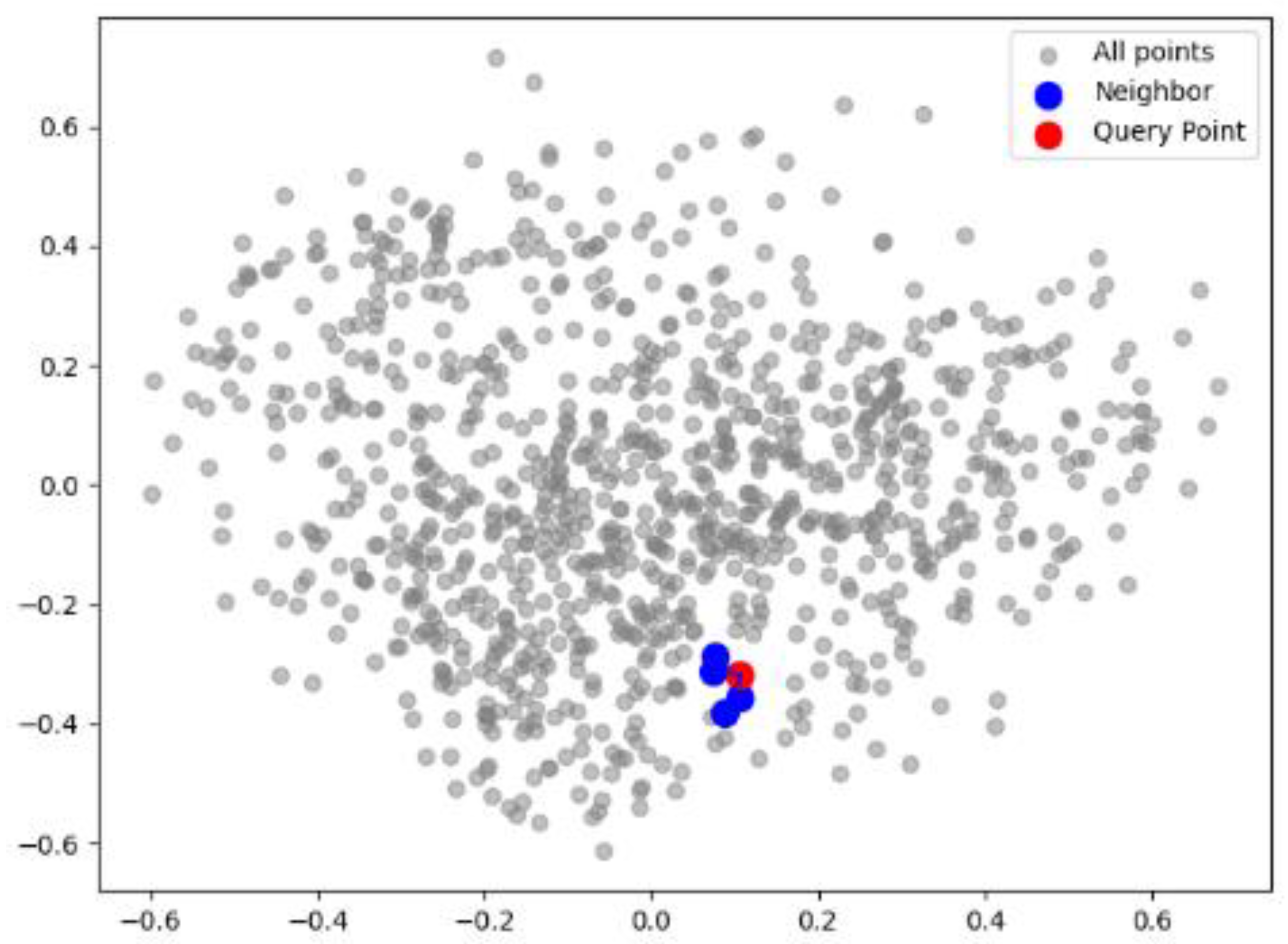
where $\mathbf{q}=(q_1,q_2,\dots ,q_D)$ is the query point, and ${\mathbf{d}}_i=(d_{i1},d_{i2},\dots ,d_{iD})$ is a node in the tree. If the subtree of the current node may contain a point closer to the query point, it is necessary to backtrack and check another subtree. The query terminates when the entire tree is traversed or when the search range is small enough and the distance is minimized. Figure 5 shows the visualization of the feature vector KD-tree constructed in this paper and its search process in the form of a two-dimensional scatter plot.

2.5. Loss Function Design

During training, the dataset consists of aerial and satellite images, with corresponding image pairs stored in the folders to form labels. In each iteration, the corresponding image pairs and their labels are used for feature extraction, and the classification probability of the images is calculated. The feature vectors are used to calculate the triplet loss to measure the relative similarity between two input samples, and the classification probability is used to calculate the cross-entropy loss to measure the distance between the model’s prediction and the true label. This paper sets the initial learning rate to 0.01 and uses an exponential decay method to gradually reduce the learning rate. The learning rate calculation formula is shown in Equation (12).

$$lr=lr\times gamm{a}^{epoch}$$

(12)

Here, epoch represents the number of training iterations, and gamma represents the learning rate adjustment factor, which is set to 0.1 in this paper. Using an appropriate learning rate can help the loss converge to the minimum more quickly and avoid getting trapped in local optima.

2.5.1. CE Loss

Cross-entropy loss is primarily used to measure the difference between the model’s predicted classification results for aerial and satellite images and their true labels, enabling the model to map the input to the correct labels. The formula for calculating cross-entropy is shown in Equation (13):

$$D_{CE}\left(O_1,O_2\right)=-{\sum }_{i}q\left(O_2^i\right)\mathit{log}p\left(O_1^i\right)$$

(13)

where $O_1$ and $O_2$ represent the model’s target output and actual output, respectively, and p and q represent the true probability distribution and the model’s predicted probability distribution, respectively. The cross-entropy losses of aerial and satellite images are added together to form a final loss function that can learn from each other, as shown in Equation (14):

$$CE Loss=D_{CE}\left(O_d,O_{d\prime }\right)+D_{CE}\left(O_s,O_{s\prime }\right)$$

(14)

where $O_d$ and $O_s$ represent the true labels of the aerial image and satellite image, respectively, and $O_{d\prime }$ and $O_{s\prime }$ represent the prediction results of the aerial image and satellite image, respectively.

2.5.2. Triplet Loss

Triplet loss is primarily used to measure the relative similarity between aerial and satellite images. By minimizing the distance between positive and query samples while maximizing the distance between negative and query samples, it ensures that the model can better distinguish between similar and dissimilar samples. The distance between two samples is calculated using the feature vectors extracted by the model, as shown in Equation (15):

$$d\left(x,y\right)={‖x-y‖}^2$$

(15)

where x and y represent the feature vectors of two samples, and ${‖\cdot ‖}^2$ represents the Euclidean distance. Let a be the feature vector of the query sample, p be the feature vector of the positive sample, and n be the feature vector of the negative sample. Then, the formula for calculating the triplet loss is as shown in Equation (16):

$$TLLoss=\mathit{max}\left(d\left(a,p\right)-d\left(a,n\right)+M,0\right)$$

(16)

where M represents the margin parameter, which is used to control the distance difference between positive and negative samples. We take M = 0.3. Because cross-view geolocation is a multi-input multi-output task, in the process of matching aerial and satellite images, we need to match images from different domains without distinguishing images from the same viewpoint. Therefore, we only calculate the triplet loss between images from different views.

3. Results

3.1. Datasets

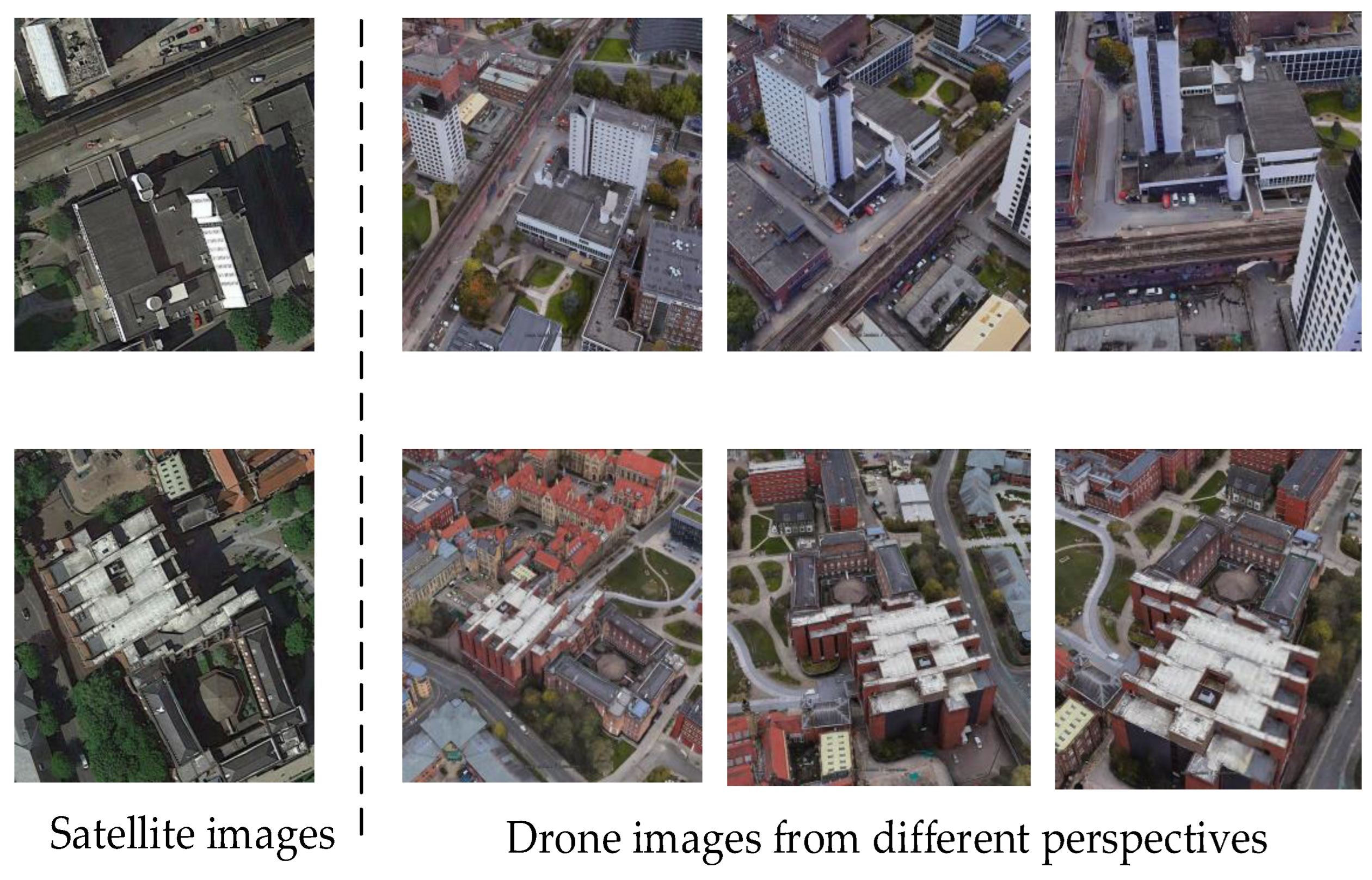
The dataset used is the University-1652 UAV multi-view geolocation dataset, which contains images from UAVs, satellites, and the ground, covering 1652 buildings from 72 universities worldwide. The training set contains 701 buildings from 33 universities, totaling 50,195 training images; the test set contains 951 buildings from 39 universities, totaling 37,855 test images. The buildings in the two sets do not overlap. Examples of images from different perspectives in the dataset are shown in Figure 6. This paper uses only UAV and satellite images for model training and performance validation.

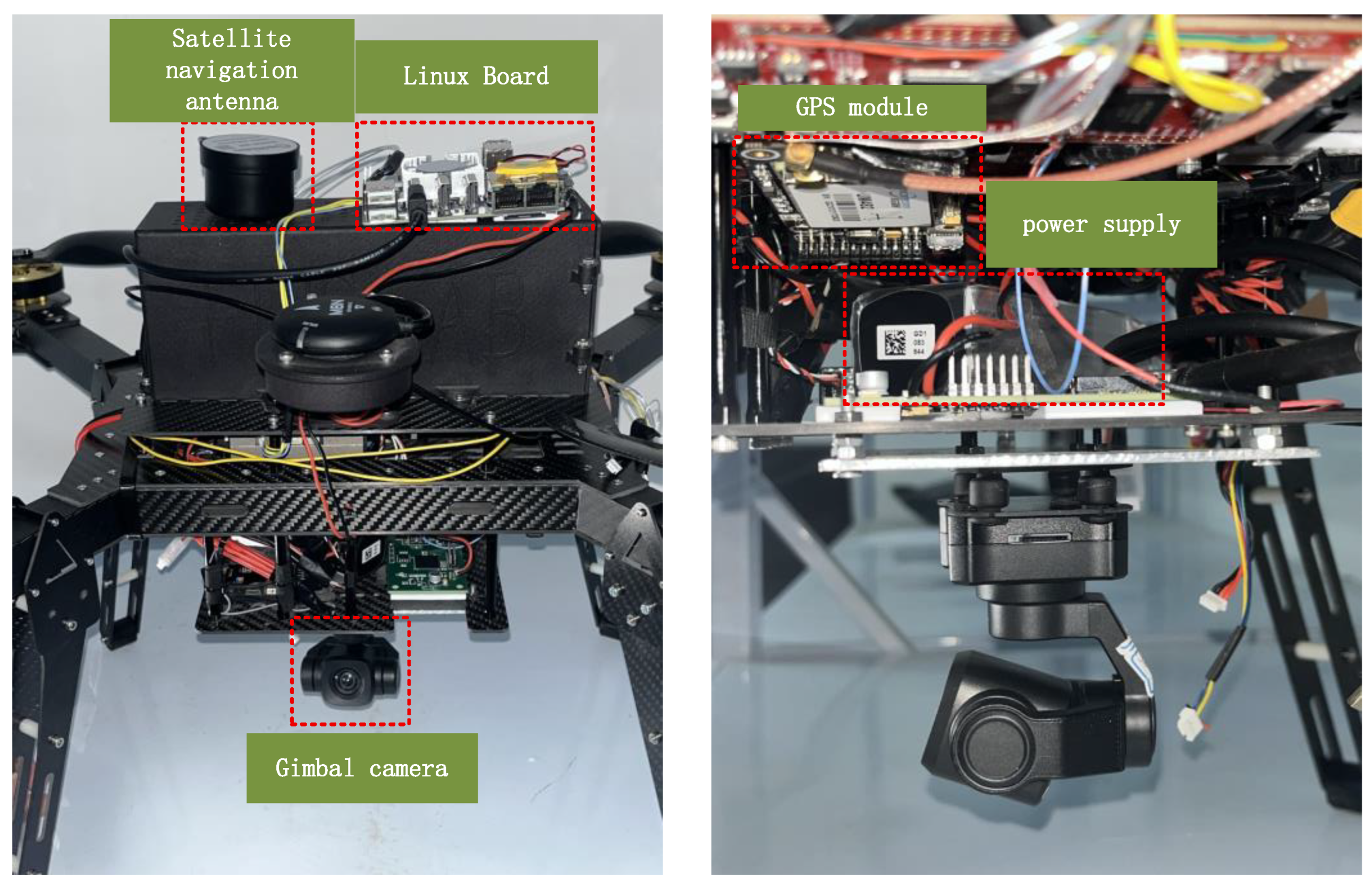
The performance of the visual scene matching navigation and positioning algorithm based on the Siamese-ViT model was evaluated based on an airborne navigation experiment. The experiment used the BeiTian BE-180 integrated GPS module as the reference benchmark, with a dynamic heading angle accuracy of 0.3°, a velocity accuracy of 0.05 m/s, and a horizontal position accuracy of 2 m. The visual sensor used in the experiment was a SiYi A8 mini monocular gimbal camera with a resolution of 1280 × 720 and a sampling frequency of 25 fps. The gimbal’s pitch, roll, and heading angle rotation ranges were —135°~45°, −30°~30°, and −160°~160°, respectively, with an angle jitter of ±0.01°. The UAV navigation test platform is shown in Figure 7.

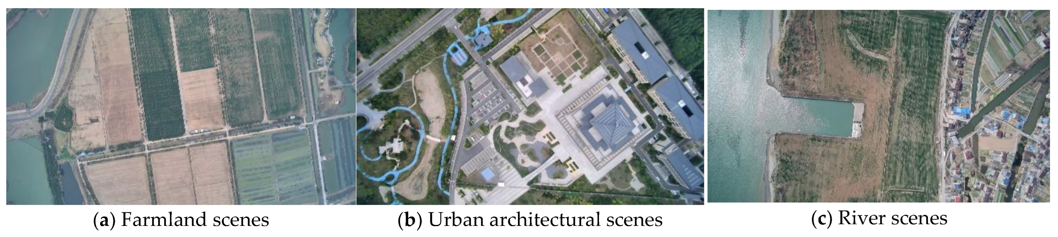
The scene types cover farmland, urban buildings, and waterways, which can characterize typical surface textures and structural features in low-altitude aerial photography missions. These three scene types (Figure 8) differ significantly in texture scale, structural complexity, and occlusion level, and can be used to analyze the adaptability of the proposed method in complex terrain environments such as farmland, waterways, and urban buildings. For satellite imagery, we selected Google Earth Level 20 imagery data.

3.2. Model Training Details

The input image size is 256 × 256 × 3. The linear mapping uses a 16 × 16 kernel with a stride of 16 and 768 kernels, resulting in a final segmentation patch size P of 16. The number of patches N after segmentation is 256, and the resulting one-dimensional vector has a dimension D of 768. Finally, a learnable position embedding is added to transform the input into a 257-dimensional sequence. The hardware platform for training the model in this paper is an Intel Core i7-12700H CPU and an RTX 3060 GPU. The neural network is built using the PyTorch 2.6, with a batch size of eight. We adopt SGD as the optimizer with momentum 0.9 and weight decay 0.0005. The initial leaning rate is 0.003 and is decayed by 0.1 in the epoch of 70 and 110, respectively.

3.3. Model Performance Verification

We employ the ViT model as the backbone network for feature extraction, introducing K-means clustering to aggregate local features. Our accuracy is compared with other models, including Contrastive Loss [36], LPN [13], FSRA [27], LPN+DWDR [37], and TransGeo [29]. Recall@k and AP are used to measure the performance of the extracted features, as shown in

Table 1. Network model comparison results.

Methods	Recall@1	Recall@5	Recall@10	AP
Contrastive Loss	52.39	78.67	85.23	57.44
LPN	75.93	84.93	90.02	79.14
FSRA	85.5	86.37	87.79	87.53
LPN+DWDR	81.51	83.25	85.63	84.11
TransGeo	84.01	85.31	88.97	86.31
Siamese_ViT	86.34	88.24	91.85	87.69

. Our proposed model achieves accuracies of 86.34%, 88.24%, 91.85%, and 87.69% for Recall@1, Recall@5, Recall@10, and AP, respectively, on the dataset. This performance surpasses other network models, showing improvements of 2.8%, 3.4%, 3.2%, and 1.6% compared to the TransFG model, and also an improvement in accuracy compared to FSRA.

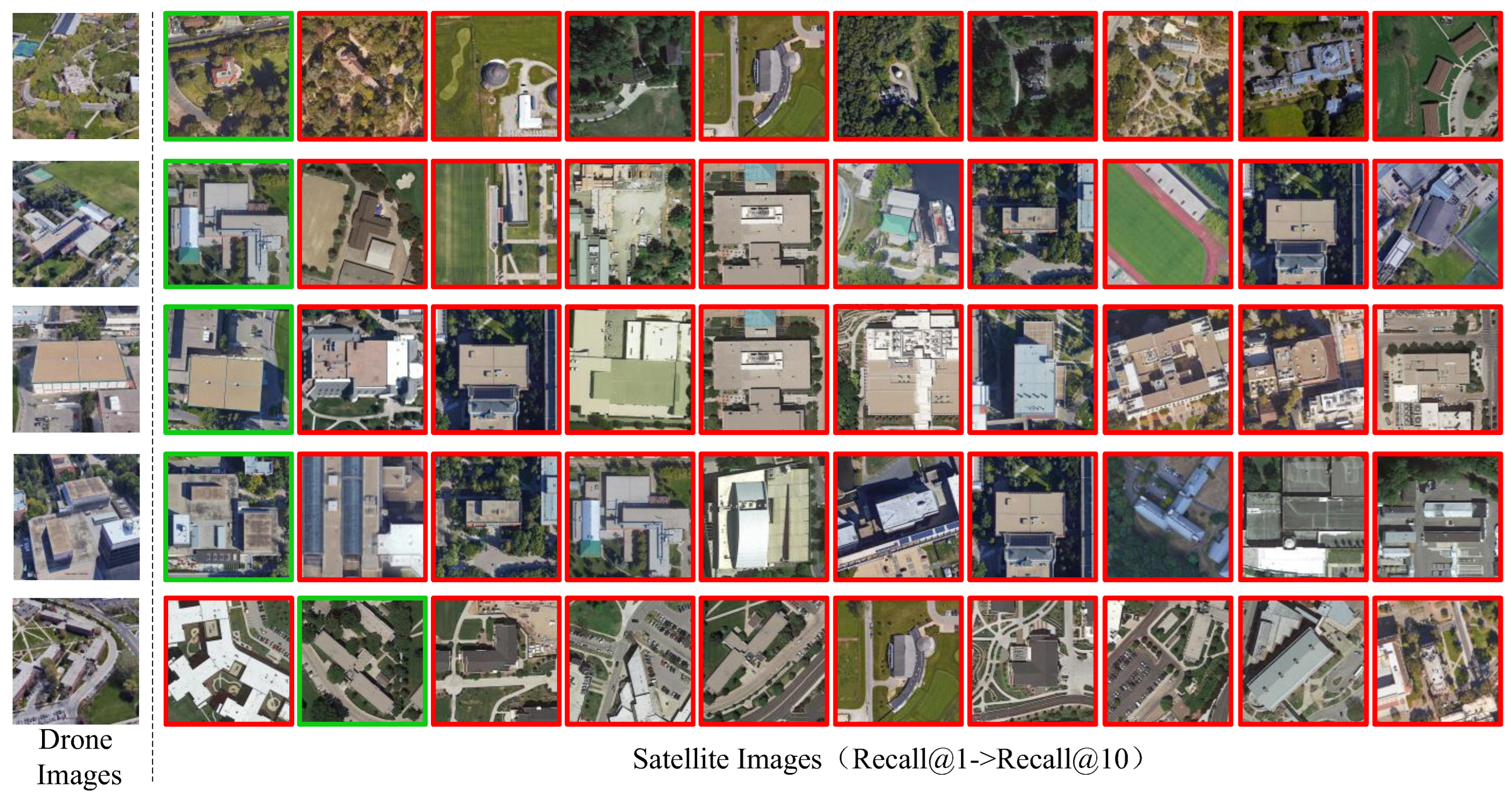
To further qualitatively analyze the model’s performance, this paper visualizes the query results and presents them intuitively on the University-1652 dataset, as shown in Figure 9. In the figure, green boxes represent correct queries, and red boxes represent incorrect queries. Since there is only one satellite image for each category in the dataset, performance can be analyzed by analyzing the position of the correct query. As can be seen from the figure, the model accurately matches the corresponding satellite image and ranks the correct query result first. Furthermore, for drone images for which no corresponding satellite image was found, the query results show a clear structural similarity between the two, validating the effectiveness of the model.

3.4. The Impact of Local Feature Aggregation Based on K-Means

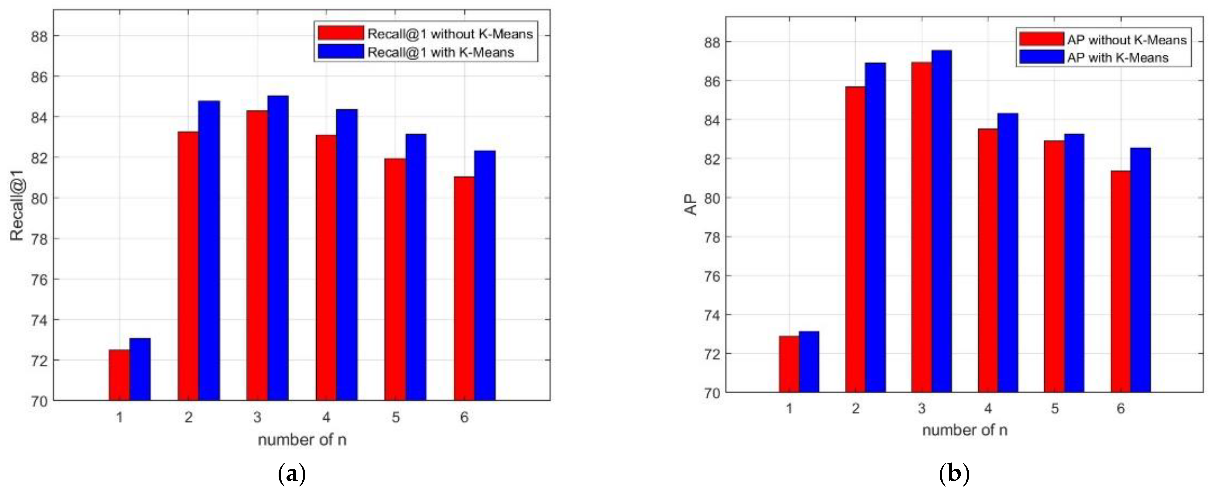
We use K-means to aggregate local features into a fixed number of “cluster centers,” which is crucial in the overall network. We experimentally validate the impact of K-means on Recall@1 and AP accuracy, as shown in Figure 10. When n = 3, Recall@1 reaches 85.05, and AP reaches 87.55. We believe that aggregating local features into three classes using K-means effectively improves matching accuracy and reduces the impact of noise on matching. When n = 2, Recall@1 reaches 84.78, and AP reaches 86.92, indicating good performance even with n = 2.

3.5. The Impact of Feature Space Dimensionality Reduction on Feature Matching

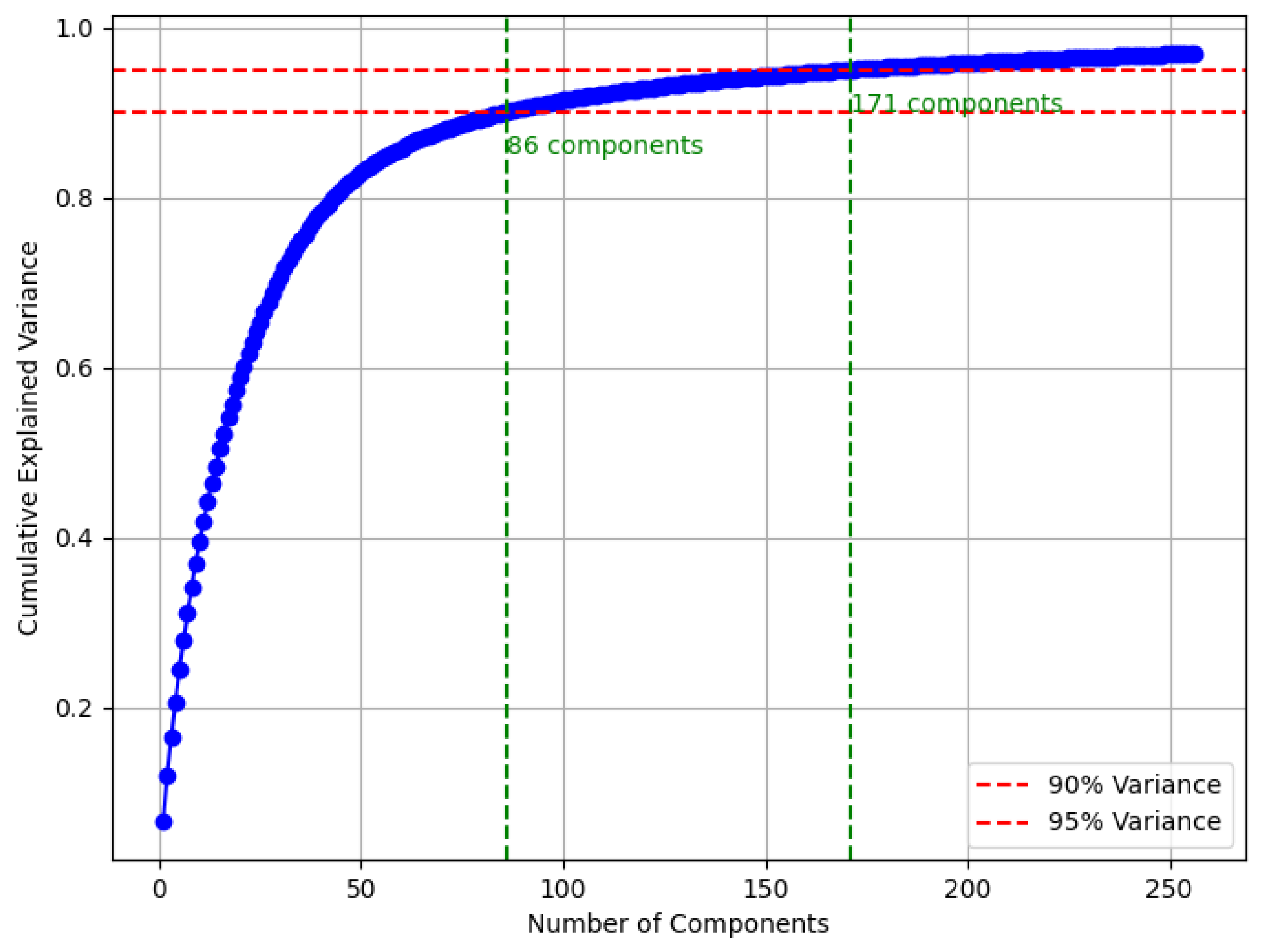
To ensure that the dimensionality-reduced feature vector retains at least 90% of its original information, the number of principal components and the cumulative explained variance were compared, as shown in Figure 11. A cumulative explained variance of 90% was achieved when the number of principal components was 86; a cumulative explained variance of 95% was achieved when the number of principal components was 171. This paper selects a principal component count of 256, meaning that the dimensionality of the reduced feature vector is 256. This achieves a cumulative explained variance of 96.89%, effectively replacing the original 2048-dimensional feature vector while preserving its original feature information.

For the feature vectors before and after dimensionality reduction, Recall@k and AP are still used to measure their performance in feature matching, and their computational efficiency is compared with that of the feature vectors before dimensionality reduction. The comparison results are shown in

Table 2. Performance comparison table before and after dimensionality reduction.

IPCA	Recall@1	Recall@5	Recall@10	AP	Time Consuming/s
Before	71.05	88.21	91.86	74.92	0.28
After	71.60	88.54	92.08	75.41	0.13

. The feature vectors after dimensionality reduction show some improvement in Recall@k and AP, achieving accuracies of 71.60%, 88.54%, 92.08%, and 75.41% for Recall@1, Recall@5, Recall@10, and AP, respectively. This is because incremental principal component analysis can align the feature vector spaces of satellite images and aerial images, making their feature spaces more consistent. In terms of computational efficiency, the feature matching time for a single image after dimensionality reduction is 0.13 s, which is about 0.15 s faster than before dimensionality reduction.

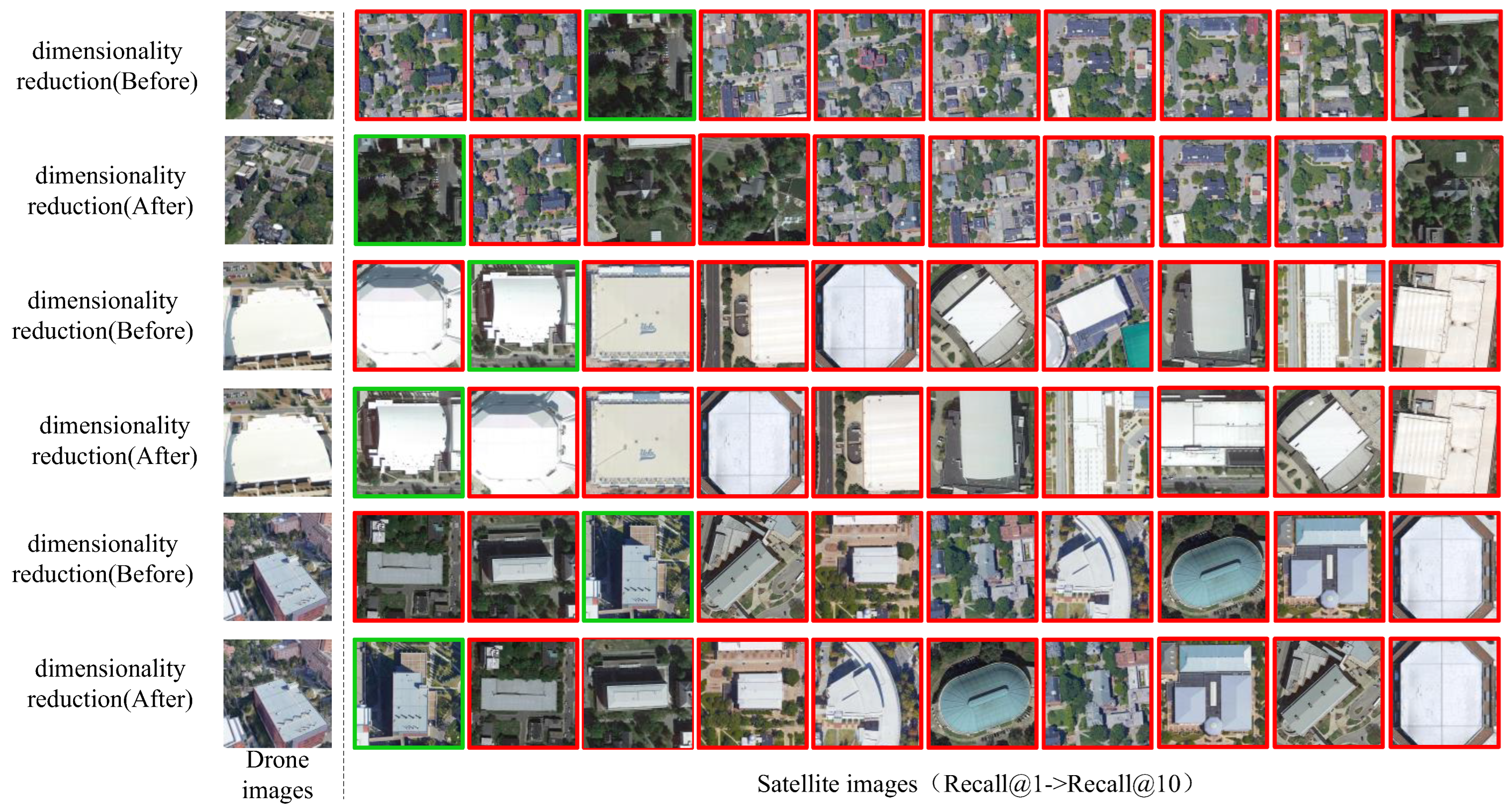
Visualizing the matching results before and after dimensionality reduction reveals that the feature matching results after dimensionality reduction are more accurate than the original results, as shown in Figure 12. The matching results after dimensionality reduction place the correct query first and significantly reduce the interference of incorrect queries. This indicates that the feature space distribution after dimensionality reduction is more compact, the aggregation of intra-class features is enhanced, and the separation of inter-class features is more obvious, thereby avoiding incorrect matching caused by feature aliasing and improving matching performance.

3.6. The Impact of KD-Tree Feature Matching on Computational Efficiency

The KD-tree structure does not affect the matching results, so we only compared its impact on computational efficiency, as shown in

Table 3. Performance comparison table before and after constructing KD tree.

KD-Tree	Time Consuming/s
Before	0.28
After	0.05

. After constructing the KD-tree structure, the feature matching time for a single image was 0.05 s, which is about 0.23 s faster than before.

The performance analysis of the overall algorithm after combining incremental principal component analysis and KD-tree structure is shown in

Table 4. Performance comparison.

Method	Recall@1	Recall@5	Recall@10	AP	Time Consuming/s
Brute-force matching	71.05	88.21	91.86	74.92	0.28
IPCA	71.60	88.54	92.08	75.41	0.13
IPCA + KD-tree	71.60	88.54	92.08	75.41	0.03

. While improving matching accuracy, the time for feature matching of a single image is 0.03 s, which is 89% higher than the original brute-force matching method’s 0.28 s.

3.7. Real Flight Test

3.7.1. Straight Path of Drone

We conducted the real-world flight tests, which results were compared with the traditional SIFT and SURF, and the navigation error of the visual scene matching localization algorithm was evaluated using MAE, RMSE, and MAX value as metrics.

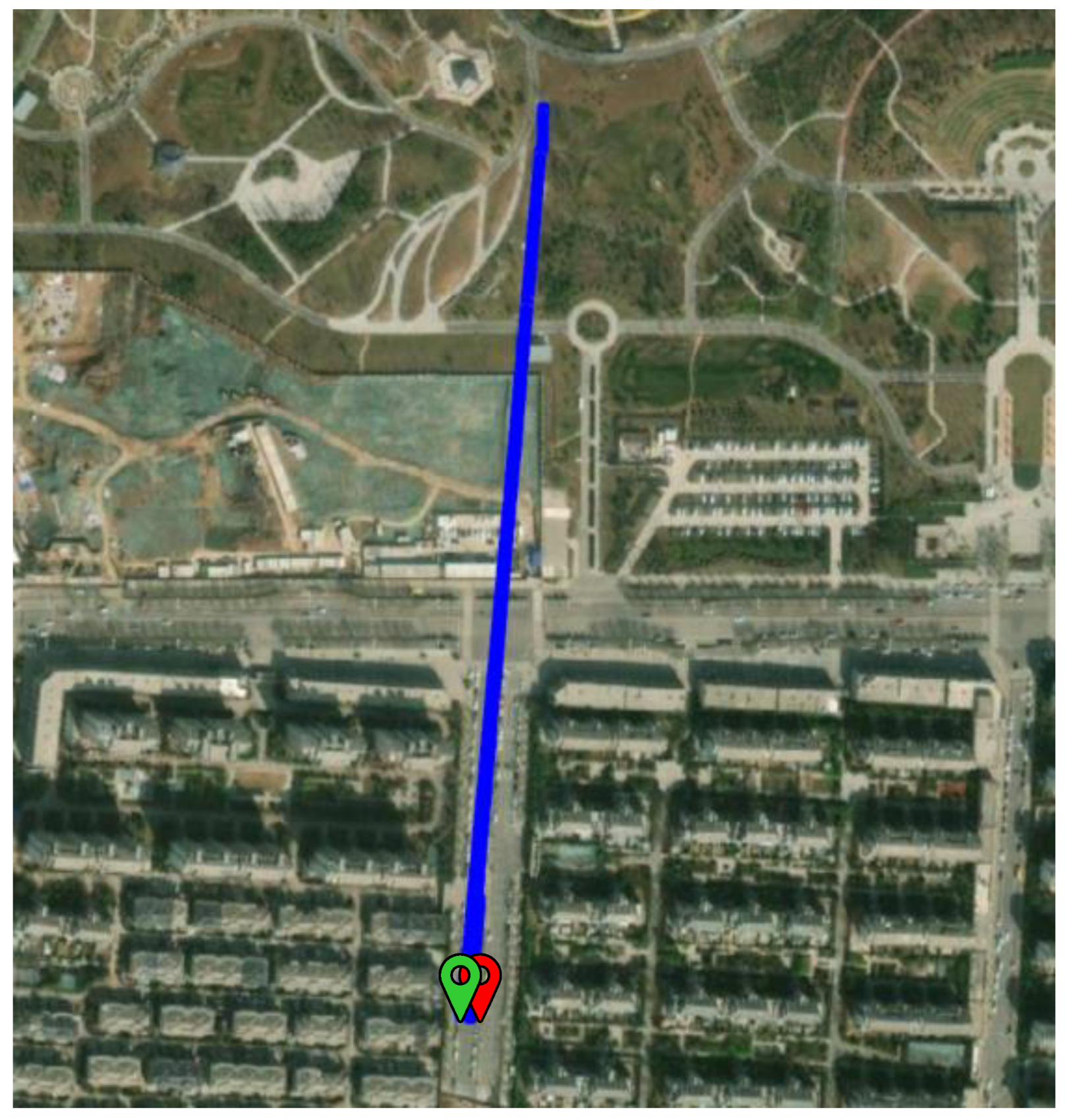
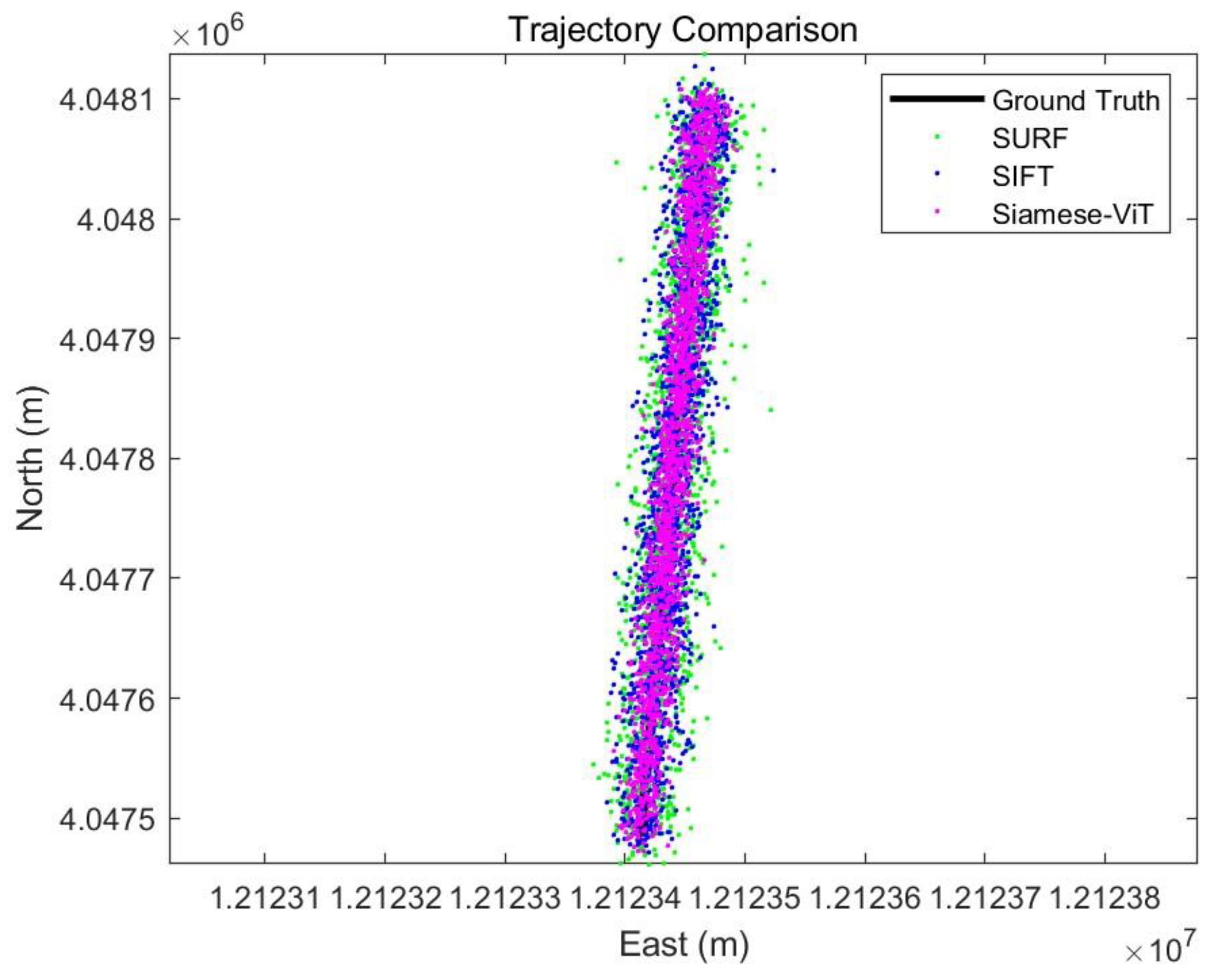
The flight time was approximately 353 s, the flight altitude was 350 m, and the image sampling frequency was 5 fps. The map trajectory is shown in Figure 13, with red and green markers representing the carrier’s position at the start and end of the experiment, respectively.

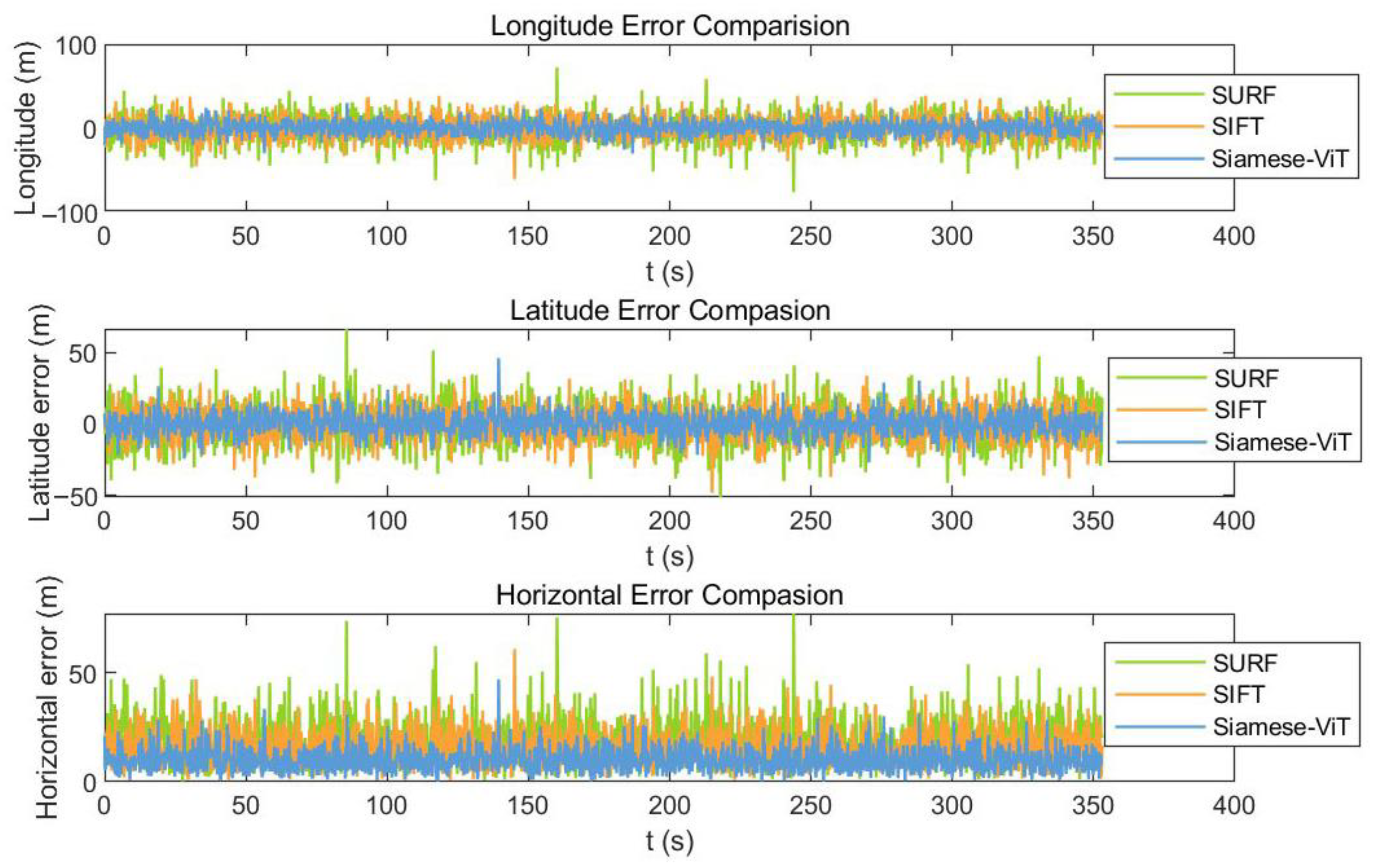
The trajectory and position error comparisons from the flight tests are shown in Figure 14 and Figure 15. The visual scene matching localization algorithm presented in this paper generally exhibits a horizontal position error better than 20 m at a flight altitude of 350 m. However, occasional error jumps of up to 50 m occur. This is because the visual scene matching localization algorithm relies on the richness of image features, and will show significant jumps when image texture features are not rich. As shown in Figure 12, the positioning points obtained by the algorithm are distributed on both sides of the actual trajectory, with occasional jump points far from the actual trajectory. This indicates that the error obtained by the visual scene matching localization algorithm is different from the inertial error and belongs to non-linear error, which is beneficial for correction of inertial device drift. With only a few abnormal fluctuations at specific time points, this indicates that the algorithm presented in this paper has ideal position accuracy.

The statistical comparison of position errors in the flight tests is shown in

Table 5. Statistical comparison of position errors in the flight tests.

Real Flight Test Type	Evaluation Indicators	Algorithm	Latitude Error/m	Longitude Error/m	Horizontal Error/m
Straight path of drone	MAE	SIFT	9.2483	10.1593	15.2996
		SURF	11.3403	12.3567	18.6705
		Siamese-ViT	6.2063	6.7552	10.1922
	RMSE	SIFT	11.6682	12.8127	17.3295
		SURF	14.3294	15.6081	21.1883
		Siamese-ViT	7.8008	8.5001	11.5371
	MAX	SIFT	86.1516	62.8514	86.2194
		SURF	80.6985	75.8746	81.9524
		Siamese-ViT	46.1594	31.0473	47.0375

. The average absolute values of the latitude, longitude, and horizontal position errors of the visual scene matching positioning algorithm in this paper are 6.2063 m, 6.7552 m, and 10.1922 m, respectively, with standard deviations of 7.8008 m, 8.5001 m, and 11.5371 m, respectively, and maximum values of 46.1594 m, 31.0473 m, and 47.0375 m, respectively.

When faced with heterogeneous image matching tasks, the Siamese-ViT combines global and local features. By extracting the overall context and spatial distribution features of the image, it enhances its adaptability to complex environmental changes. Therefore, its latitude, longitude, and horizontal error fluctuations are relatively small. In contrast, the SIFT and SURF algorithms, which rely on feature point detection results, are easily affected by changes in ambient lighting and weather, leading to a significant increase in matching error and obvious jump points. Compared with the SIFT and SURF algorithms, the visual scene matching localization algorithm in this paper improves the average absolute values of latitude, longitude, and horizontal position errors by 32.89%, 33.51%, and 33.38%, and 45.27%, 45.33%, and 45.41%, respectively; the mean square errors by 33.14%, 33.66%, and 33.43%, and 45.56%, 45.54%, and 45.55%, respectively; and the maximum values by 46.42%, 50.60%, and 52.40%, and 42.80%, 59.08%, and 42.60%, respectively.

3.7.2. Irregular Path of Drone

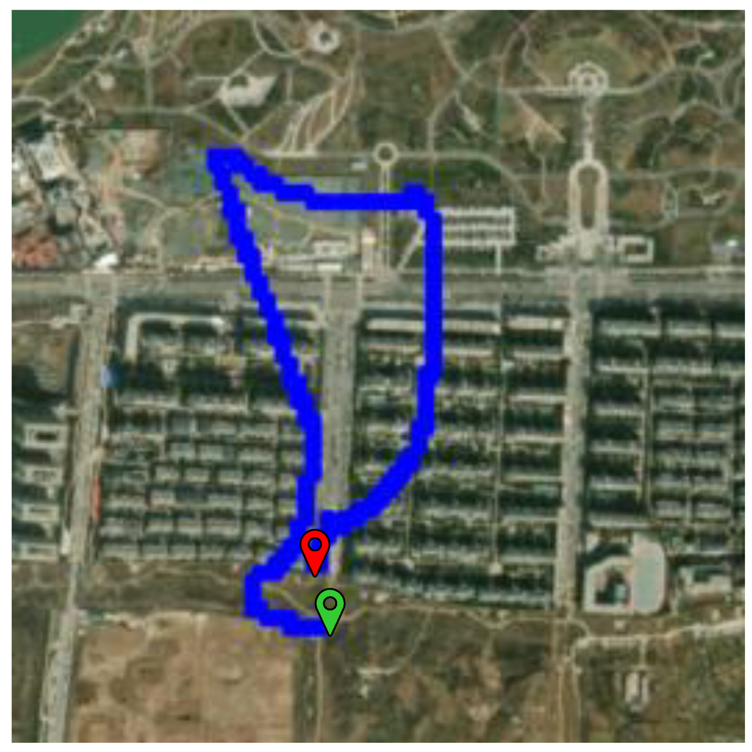
The flight time was approximately 350 s, the flight altitude was 200 m, and the image sampling frequency was 1 fps. The map trajectory is shown in Figure 16.

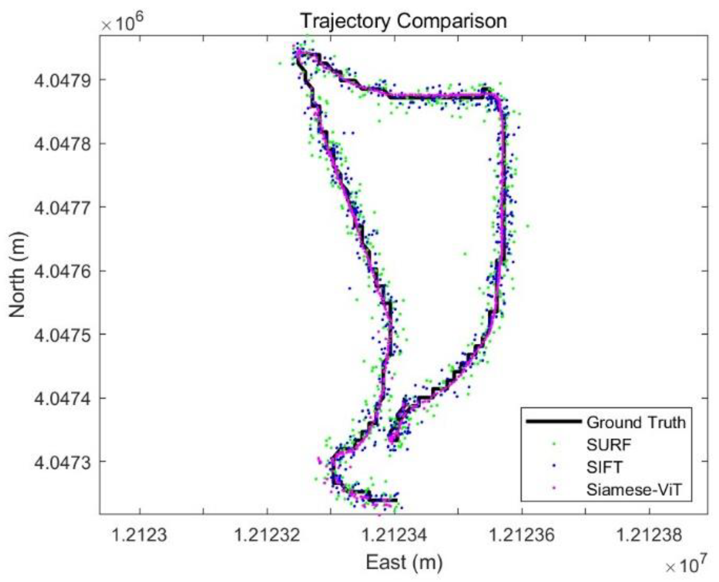
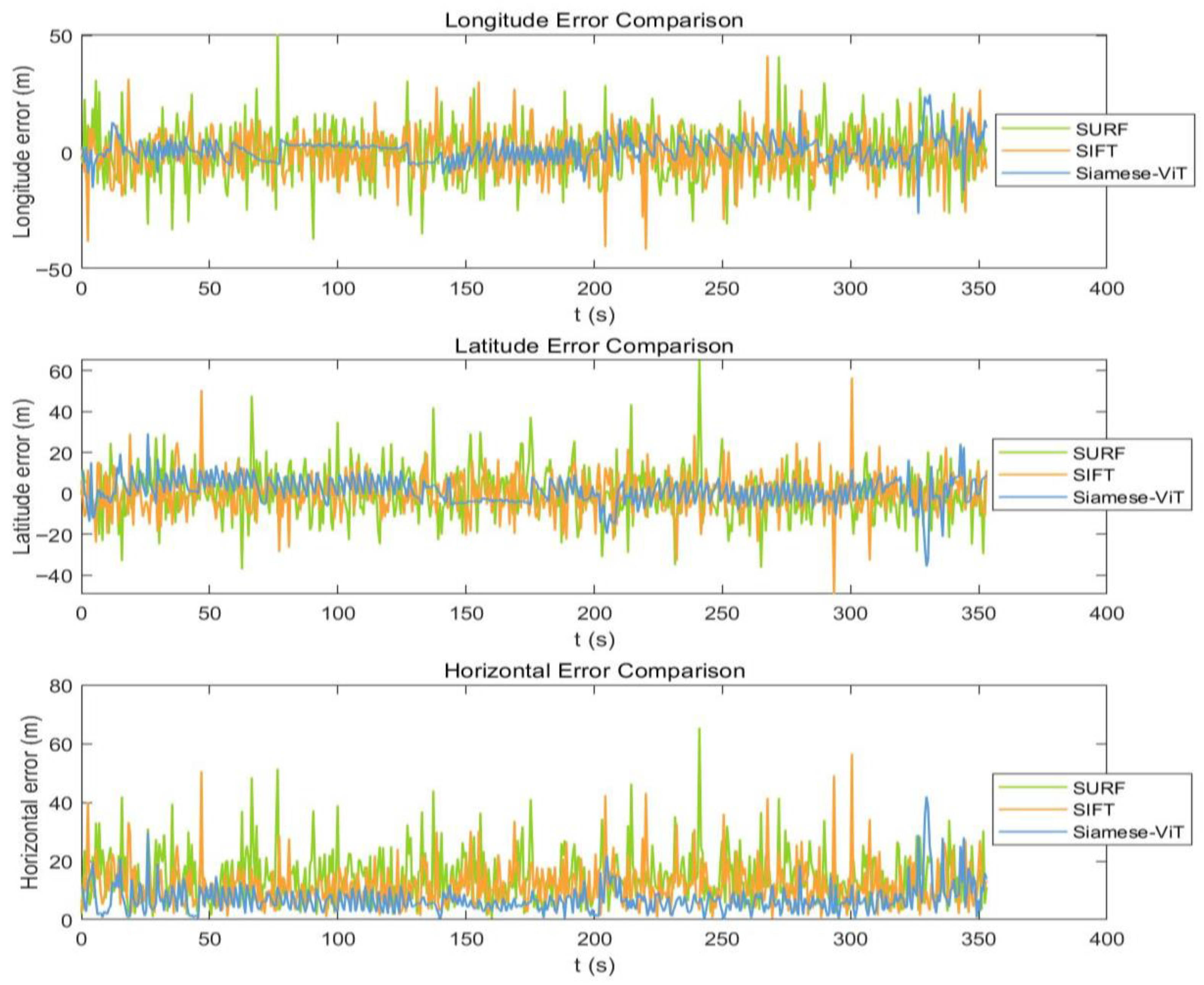
The trajectory and position error comparisons from the flight tests are shown in Figure 17 and Figure 18. The visual scene matching positioning algorithm presented in this paper exhibits an overall horizontal position error better than 15 m at a flight altitude of 200 m. Since the overall position error is controlled within 5% of the altitude, with only a few abnormal fluctuations at specific time points, this indicates that the algorithm in this paper possesses ideal position accuracy.

The statistical comparison of position errors in the flight tests is shown in

Table 6. Statistical comparison of position errors in the irregular path flight tests.

Real Flight Test Type	Evaluation Indicators	Algorithm	Latitude Error/m	Longitude Error/m	Horizontal Error/m
Irregular path of drone	MAE	SIFT	7.2511	7.1905	11.5583
		SURF	9.2044	9.0961	14.4325
		Siamese-ViT	4.9685	3.8587	6.8526
	RMSE	SIFT	9.8681	9.6123	13.7759
		SURF	12.2220	11.6697	16.8985
		Siamese-ViT	6.5794	5.1902	8.3801
	MAX	SIFT	56.5541	41.6551	56.5865
		SURF	65.1151	50.4499	65.3702
		Siamese-ViT	35.6408	26.2714	41.9643

. The average absolute values of the latitude, longitude, and horizontal position errors of the visual scene matching positioning algorithm in this paper are 4.9685 m, 3.8587 m, and 6.8526 m, respectively; the standard deviations are 6.5794 m, 5.1902 m, and 8.3801 m, respectively; and the maximum values are 35.6408 m, 26.2714 m, and 41.9643 m, respectively.

Compared to the SIFT and SURF algorithms, the visual scene matching localization algorithm presented in this paper improves the mean absolute values of latitude, longitude, and horizontal position errors by 31.48%, 46.34%, and 40.71%, and 46.02%, 57.58%, and 52.52%, respectively; the mean square errors by 33.33%, 46.00%, and 39.17%, and 46.17%, 55.52%, and 50.41%, respectively; and the maximum improvements by 37.03%, 36.93%, and 34.84%, and 45.26%, 47.93%, and 35.81%, respectively.

4. Discussion

To address the issue of decreased positioning accuracy in visual scene matching systems due to environmental differences and other factors, we established an end-to-end Siamese-ViT-based feature matching framework, significantly improving the system’s robustness. In feature extraction, we improved the ViT model to generate robust feature representation vectors and introduced clustering to adapt to specific scene matching tasks, achieving a Recall@1 metric superior to 86.34%. For feature matching, we used IPCA and KD-tree structures for fast feature retrieval, improving matching time by 89%. According to airborne navigation tests, our algorithm achieved an average absolute value of 6.2063 m for latitude error, 6.7552 m for longitude error, and 10.1922 m for horizontal error at a flight altitude of 350 m. Therefore, our algorithm demonstrates ideal overall positioning accuracy. However, in low-texture environments, fewer image features lead to difficulties in image matching, negatively impacting localization results. In the future, we will investigate image matching and localization methods for low-texture environments to better address UAV localization problems in real-world environments.

5. Conclusions

To address the navigation challenges in complex environments with satellite denial, we propose a Siamese-ViT-based visual navigation method that integrates local fine-grained information with global semantic information and that uses IPCA to reduce the dimensionality of the feature space, providing a feasible solution for the autonomous flight of unmanned aerial vehicles (UAVs). Our method outperforms other models in both Recall and AP metrics. In real-world environments, we collected drone images from various complex scenarios to validate the algorithm’s effectiveness. Experimental results demonstrate that our method achieves ideal positioning accuracy.

References

1. Lowe, D.G. Distinctive Image Features from Scale-Invariant Keypoints. Int. J. Comput. Vis. 2004, 60, 91–110. [Google Scholar] [CrossRef]
2. Bay, H.; Tuytelaars, T.; Van Gool, L. Surf: Speeded up robust features. Eur. Conf. Comput. Vis. 2006, 3951, 404–417. [Google Scholar]
3. Rublee, E.; Rabaud, V.; Konolige, K.; Bradski, G. ORB: An efficient alternative to SIFT or SURF. In Proceedings of the IEEE International Conference on Computer Vision (ICCV), Barcelona, Spain, 6–13 November 2011; pp. 2564–2571. [Google Scholar]
4. Lepetit, V.; Moreno-Noguer, F.; Fua, P. EPnP: An accurate O(n) solution to the PnP problem. Int. J. Comput. Vis. 2008, 81, 155–166. [Google Scholar] [CrossRef]
5. Besl, P.J.; McKay, N.D. Method for registration of 3D shapes. IEEE Trans. Pattern Anal. Mach. Intell. (TPAMI) 1992, 14, 239–256. [Google Scholar] [CrossRef]
6. Cummins, M.; Newman, P. FAB-MAP: Probabilistic localization and mapping in the space of appearance. Int. J. Robot. Res. 2008, 27, 647–665. [Google Scholar] [CrossRef]
7. Milford, M.; Wyeth, G. SeqSLAM: Visual route-based navigation for sunny summer days and stormy winter nights. In Proceedings of the IEEE International Conference on Robotics and Automation (ICRA), St. Paul, MN, USA, 14–18 May 2012; pp. 1643–1649. [Google Scholar]
8. Wang, Z.; Shi, D.; Qiu, C.; Jin, S.; Li, T.; Shi, Y.; Liu, Z.; Qiao, Z. Sequence matching for image-based uav-to-satellite geolocalization. IEEE Trans. Geosci. Remote Sens. 2024, 62, 5607815. [Google Scholar] [CrossRef]
9. Baykal, F.; Gedik, M.İ.; Reyes-Aldasoro, C.C.; Karabağ, C. Image Matching for UAV Geolocation: Classical and Deep Learning Approaches. J. Imaging 2025, 11, 409. [Google Scholar] [CrossRef] [PubMed]
10. Hu, S.; Feng, M.; Nguyen, R.M.H.; Lee, G.H. CVM-Net: Cross-view matching network for image-based ground-to-aerial geo-localization. In Proceedings of the IEEE/CVF Conference on Computer Vision and Pattern Recognition (CVPR), Salt Lake City, UT, USA, 18–22 June 2018; pp. 7258–7267. [Google Scholar]
11. Shi, Y.; Liu, L.; Yu, X.; Li, H. Spatial-Aware Feature Aggregation for Image based Cross-View Geo-Localization. In Proceedings of the 33rd International Conference on Neural Information Processing Systems, Vancouver, BC, Canada, 8–14 December 2019; p. 32. [Google Scholar]
12. Zheng, Z.; Wei, Y.; Yang, Y. University-1652: A Multi-view Multi-source Benchmark for Drone-based Geo-localization. In Proceedings of the 28th ACM International Conference on Multimedia, Seattle, WA, USA, 12–16 October 2020; pp. 1395–1403. [Google Scholar]
13. Wang, T.; Zheng, Z.; Yan, C.; Zhang, J.; Sun, Y.; Zheng, B.; Yang, Y. Each Part Matters: Local Patterns Facilitate Cross-View Geo-Localization. IEEE Trans. Circuits Syst. Video Technol. 2022, 32, 867–879. [Google Scholar] [CrossRef]
14. Arandjelović, R.; Gronat, P.; Torii, A.; Pajdla, T.; Sivic, J. NetVLAD: CNN architecture for weakly supervised place recognition. In Proceedings of the IEEE Conference on Computer Vision and Pattern Recognition (CVPR), Las Vegas, NV, USA, 27–30 June 2016; pp. 5297–5307. [Google Scholar]
15. Noh, H.; Araujo, A.; Sim, J.; Weyand, T.; Han, B. Large-Scale Image Retrieval with Attentive Deep Local Features. In Proceedings of the IEEE International Conference on Computer Vision, Venice, Italy, 22–29 October 2017; pp. 3456–3465. [Google Scholar]
16. Hausler, S.; Garg, S.; Xu, M.; Milford, M.; Fischer, T. Patch-NetVLAD: Multi-scale fusion of locally-global descriptors for place recognition. In Proceedings of the IEEE/CVF Conference on Computer Vision and Pattern Recognition (CVPR), Virtual Conference, 19–25 June 2021; pp. 14141–14152. [Google Scholar]
17. Berton, G.; Masone, C.; Caputo, B. Rethinking Visual Geo-localization for Large-Scale Applications. In Proceedings of the IEEE/CVF Conference on Computer Vision and Pattern Recognition, New Orleans, LA, USA, 19–24 June 2022; pp. 4878–4888. [Google Scholar]
18. Ali-bey, A.; Chaib-draa, B.; Giguère, P. MixVPR: Feature Mixing for Visual Place Recognition. In Proceedings of the IEEE/CVF Winter Conference on Applications of Computer Vision, Waikoloa, HI, USA, 3–7 January 2023; pp. 2998–3007. [Google Scholar]
19. Liao, Y.; Su, J.; Ma, D.; Niu, C. Uav-satellite cross-view image matching based on adaptive threshold-guided ring partitioning framework. Remote Sens. 2025, 17, 2448. [Google Scholar] [CrossRef]
20. Li, M.; Wang, Z.; Huo, G.; Chen, W.; Zhao, X. A Deep Learning Framework with Geographic Information Adaptive Loss for Remote Sensing Images based UAV Self-Positioning. arXiv 2025, arXiv:2502.16164. [Google Scholar] [CrossRef]
21. Tian, Y.; Chen, C.; Shah, M. Cross-view image matching for geo-localization in urban environments. In Proceedings of the IEEE Conference on Computer Vision and Pattern Recognition, Honolulu, HI, USA, 21–26 July 2017; pp. 3608–3616. [Google Scholar]
22. Tian, X.; Shao, J.; Ouyang, D.; Shen, H.T. UAV-satellite view synthesis for cross-view geo-localization. IEEE Trans. Circuits Syst. Video Technol. 2021, 32, 4804–4815. [Google Scholar] [CrossRef]
23. Zhang, X.; Shore, T.; Chen, C.; Mendez, O.; Hadfield, S.; Wshah, S. VICI: VLM-Instructed Cross-view Image-localisation. In Proceedings of the 3rd International Workshop on UAVs in Multimedia: Capturing the World from a New Perspective, Dublin, Ireland, 27–31 October 2025; pp. 21–25. [Google Scholar]
24. Zhang, H.; Liu, Y.; Kuang, Z. SkyLink: Unifying Street-Satellite Geo-Localization via UAV-Mediated 3D Scene Alignment. In Proceedings of the 3rd International Workshop on UAVs in Multimedia: Capturing the World from a New Perspective, Dublin, Ireland, 27 October 2025; pp. 26–30. [Google Scholar]
25. Ji, Y.; He, B.; Tan, Z.; Wu, L. MMGeo: Multimodal Compositional Geo-Localization for UAVs. In Proceedings of the IEEE/CVF International Conference on Computer Vision, Honolulu, HI, USA, 19–23 October 2025; pp. 25165–25175. [Google Scholar]
26. Dosovitskiy, A.; Beyer, L.; Kolesnikov, A.; Weissenborn, D.; Zhai, X.; Unterthiner, T.; Dehghani, M.; Minderer, M.; Heigold, G.; Gelly, S.; et al. An image is worth 16×16 words: Transformers for image recognition at scale. In Proceedings of the International Conference on Learning Representations (ICLR), Virtual Conference, 3–7 May 2021; pp. 3–7. [Google Scholar]
27. Dai, M.; Hu, J.; Zhuang, J.; Zheng, E. A Transformer-Based Feature Segmentation and Region Alignment Method for UAV-View Geo-Localization. IEEE Trans. Circuits Syst. Video Technol. 2022, 32, 4376–4389. [Google Scholar] [CrossRef]
28. Yang, H.; Lu, X.; Zhu, Y. Cross-view geo-localization with layer-to-layer transformer. Neural Inf. Process. Syst. 2021, 34, 29009–29020. [Google Scholar]
29. Zhu, S.; Sha, M.h; Chen, C. TransGeo: Transformer Is All You Need for Cross-View Image Geo-Localization. In Proceedings of the IEEE/CVF Conference on Computer Vision and Pattern Recognition (CVPR), New Orleans, LA, USA, 19–24 June 2022; pp. 1162–1171. [Google Scholar]
30. Deuser, F.; Habel, K.; Oswald, N. Sample4Geo: Hard Negative Sampling for Cross-View Geo-Localisation. In Proceedings of the IEEE/CVF International Conference on Computer Vision (ICCV), Paris, France, 2–6 October 2023; pp. 16847–16856. [Google Scholar]
31. Liu, Z.; Lin, Y.; Cao, Y.; Hu, H.; Wei, Y.; Zhang, Z.; Lin, S.; Guo, B. Swin Transformer: Hierarchical vision transformer using shifted windows. In Proceedings of the IEEE International Conference on Computer Vision (ICCV), Virtual Conference, 11–17 October 2021; pp. 10012–10022. [Google Scholar]
32. Kannan, S.S.; Min, B.-C. PlaceFormer: Transformer-Based Visual Place Recognition Using Multi-Scale Patch Selection and Fusion. IEEE Robot. Autom. Lett. 2024, 9, 6552–6559. [Google Scholar] [CrossRef]
33. Tian, Z.; Huang, W.; Chen, Z.; Sun, X.W. Robust Visual Localization via Semantic-Guided Multi-Scale Transformer. arXiv 2025, arXiv:2506.08526. [Google Scholar]
34. Grainge, O.; Milford, M.; Bodala, I.; Ramchurn, S.D.; Ehsan, S. TAT-VPR: Ternary Adaptive Transformer for Dynamic and Efficient Visual Place Recognition. arXiv 2025, arXiv:2505.16447. [Google Scholar] [CrossRef]
35. Zhang, F.; Ren, H.; Ma, F.; Yin, Q.; Zhou, Y. SMGeo: Cross-View Object Geo-Localization with Grid-Level Mixture-of-Experts. arXiv 2025, arXiv:2511.14093. [Google Scholar]
36. Deng, W.; Zheng, L.; Ye, Q.; Kang, G.; Yang, Y.; Jiao, J. Image-image domain adaptation with preserved self-similarity and domain dissimilarity for person re-identification. In Proceedings of the IEEE Conference on Computer Vision and Pattern Recognition, Salt Lake City, UT, USA, 18–22 June 2018; pp. 994–1003. [Google Scholar]
37. Wang, T.; Zheng, Z.; Zhu, Z.; Gao, Y.; Yang, Y.; Yan, C. Learning Cross-view Geo-localization Embeddings via Dynamic Weighted Decorrelation Regularization. IEEE Trans. Geosci. Remote Sens. 2024, 62, 5647112. [Google Scholar] [CrossRef]
Figure 1. Overall architecture of Siamese-ViT.
Remotesensing 18 01556 g001
Figure 2. Transformer encoder.
Remotesensing 18 01556 g002
Figure 3. Global feature transformation and classification.
Remotesensing 18 01556 g003
Figure 4. (a) Structure of K-means. (b) The heatmap of the spatial distribution. (* is cls_Token).
Remotesensing 18 01556 g004
Figure 5. Visualization of KD-tree and its search process.
Remotesensing 18 01556 g005
Figure 6. Example images from different perspectives in the University-1652 dataset.
Remotesensing 18 01556 g006
Figure 7. UAV navigation test platform.
Remotesensing 18 01556 g007
Figure 8. Image data types acquired during flight tests.
Remotesensing 18 01556 g008
Figure 9. Query results.
Remotesensing 18 01556 g009
Figure 10. Comparison of the effects of K-means on Recall@1 and AP. (a) The effect of the number of n on the accuracy of Recall@1. (b) The effect of the number of n on the accuracy of AP.
Remotesensing 18 01556 g010
Figure 11. Cumulative explained variance. The green line is the number of components. The blue line represents the cumulative explained variance corresponding to the number of all principal components.
Remotesensing 18 01556 g011
Figure 12. Visualizing the matching results before and after dimensionality reduction. The green rectangles indicate the correct query results. The red rectangles indicate the incorrect query results.
Remotesensing 18 01556 g012
Figure 13. Map trajectory of straight path.
Remotesensing 18 01556 g013
Figure 14. Trajectory comparisons of straight path.
Remotesensing 18 01556 g014
Figure 15. Position error comparisons of straight path.
Remotesensing 18 01556 g015
Figure 16. Map trajectory of irregular flight path.
Remotesensing 18 01556 g016
Figure 17. Trajectory comparisons of irregular path.
Remotesensing 18 01556 g017
Figure 18. Position error comparisons of irregular path.
Remotesensing 18 01556 g018