HW-OPINN: A Heat Wave-Optimized Physics-Informed Neural Network for Marine Heatwave Prediction

Highlights

What are the main findings?

• A Heat Wave-Optimized Physics-Informed Neural Network (HW-OPINN) is proposed that integrates ocean mixed-layer heat budget dynamics with adaptive deep learning, achieving a test MSE of 0.009138 and RMSE of 0.0956 °C, representing improvements of 43.9% and 25.1% over the ConvLSTM baseline and 44.8% and 25.7% over standard PINN, respectively.
• The framework successfully reproduces the spatial heterogeneity of marine heatwave characteristics in the Mediterranean Sea, achieving the lowest MAE for event frequency (0.822 events/year) and mean duration (3.999 days) among all compared methods.

What are the implications of the main findings?

• The dual-adaptive optimization strategy—combining Boltzmann-based collocation point sampling, region-specific adaptive weight optimization, and Bayesian hyperparameter tuning—provides a systematic methodology for balancing physical constraints against data fitting in Physics-Informed neural networks.
• This work demonstrates the potential of integrating physical knowledge with data-driven methods for reliable extreme ocean event prediction, supporting climate adaptation and marine resource management.

Abstract

Marine heatwaves (MHWs) are prolonged extreme warming events that pose severe threats to marine ecosystems and coastal communities, necessitating reliable prediction capabilities for climate adaptation and marine resource management. Traditional numerical models, while physically grounded, are constrained by computational costs and error accumulation, whereas purely data-driven approaches often lack physical consistency and generalize poorly to extreme events. To address these challenges, this study proposes a Heat Wave-Optimized Physics-Informed Neural Network (HW-OPINN) that synergistically integrates ocean mixed-layer heat budget dynamics with adaptive deep learning techniques. The proposed framework introduces three methodological innovations. First, an adaptive sampling strategy grounded in Boltzmann distribution theory dynamically reallocates physical collocation points toward high-gradient regions based on historical loss patterns. Second, a residual-based adaptive weight update mechanism automatically modulates physical constraint contributions across spatially heterogeneous regions during training. Third, a Bayesian optimization framework employing Gaussian process surrogates systematically balances physical constraints against data fitting objectives. The framework is validated through comprehensive experiments in the Mediterranean Sea using multi-source reanalysis data spanning over two decades. Results demonstrate that HW-OPINN achieves superior performance in sea surface temperature (SST) prediction, with a test MSE of 0.009138 and RMSE of 0.095595, representing improvements of 43.9% and 25.1%, respectively, compared to the ConvLSTM baseline (MSE: 0.016275, RMSE: 0.127575), and 44.8% and 25.7% improvements over standard PINN (MSE: 0.016550, RMSE: 0.128661). Based on the predicted SST fields, the model successfully reproduces the spatial heterogeneity of key MHW characteristics, including event frequency, duration, and intensity distributions, demonstrating its effectiveness for downstream MHW detection and analysis.

1. Introduction

Marine heatwaves (MHWs) represent one of the most striking manifestations of climate change in oceanic systems, characterized by prolonged periods of anomalously high temperatures lasting from several days to months in specific marine regions [1,2]. In recent decades, the frequency and intensity of MHWs have increased significantly worldwide, leading to multiple mass mortality events among marine organisms and adversely impacting coastal fisheries and tourism industries [3,4,5,6,7,8]. These observations underscore the critical importance of accurately predicting MHW occurrence, duration, and intensity for effective marine resource management and climate change adaptation strategies.

However, the formation and development of MHWs involve complex and diverse processes influenced by air–sea interface heat flux [9], horizontal temperature advection [10], vertical mixing, and large-scale climate modes including the El Niño-Southern Oscillation (ENSO) [11,12], the Indian Ocean Dipole (IOD), and the North Atlantic Oscillation (NAO) [13]. These dynamic processes exhibit pronounced nonlinear characteristics and regional heterogeneity, rendering accurate MHW prediction particularly challenging. Furthermore, while MHWs manifest prominently at the sea surface, subsurface temperature anomalies exert significant impacts on marine ecosystems and air–sea coupling processes [14,15]. Yet, existing observational capabilities and data acquisition systems inadequately cover the multi-scale, multi-depth spatiotemporal distribution of sea temperatures, further amplifying prediction uncertainty.

In response to these challenges, the scientific community primarily relies on two types of methods for MHW prediction: numerical simulation and data-driven approaches. Since MHWs are primarily characterized by anomalous changes in sea surface temperature (SST), accurately predicting the spatiotemporal evolution of SST is crucial for studying MHWs. Numerical simulation methods play a vital role in marine environmental research, helping to understand the mechanisms underlying MHWs and enabling the study of spatiotemporal evolution of SST and other environmental variables. Traditional approaches have primarily relied on physics-based numerical simulations, with studies by Merryfield et al. [16], Saha et al. [17], and Vecchi et al. [18] demonstrating how dynamical prediction systems can simulate complex ocean-atmosphere interaction processes. Jacox et al. [19] utilized eight global coupled climate prediction systems to forecast MHWs in the California Current System up to eight months in advance; however, dynamical models showed limited predictive skill for rapidly developing heatwave stages in mid-latitude regions. Oliver et al. [20] analyzed the unprecedented 2015/16 Tasman Sea marine heatwave, revealing that current numerical models still face challenges in predicting such complex events driven by multiple interacting factors. When studying highly nonlinear [21] and cross-scale [22] MHWs, due to the combined effects of complex air–sea coupling and multi-scale dynamical processes [23], numerical models often require substantial computational costs and extremely fine parameter tuning. Once long-term simulations or nonlinear process handling becomes insufficient [24], error accumulation rapidly amplifies, significantly reducing the ability to represent actual sea temperature evolution. Furthermore, these models mostly rely on idealized assumptions regarding sea surface and atmospheric boundary conditions, limiting their accuracy under transient or severely perturbed scenarios. More importantly, the performance of numerical models is often constrained by human understanding of relevant physical mechanisms and processes; when our knowledge of MHW occurrence mechanisms remains incomplete or contains blind spots, numerical models struggle to transcend the limitations of existing theoretical frameworks, making it difficult to accurately capture the dynamic changes of the real world.

In contrast, with the rapid development of big data and high-performance computing technologies, machine learning (especially deep learning) has demonstrated strong potential in processing high-dimensional, multi-source data [25,26]. Early research primarily focused on SST prediction, achieving promising results using methods such as Recurrent Neural Networks (RNNs), Long Short-Term Memory networks (LSTMs), and Convolutional Neural Networks (CNNs) [27,28,29]. Ham and colleagues [30,31] developed CNN-based methods that achieved predictions of the Niño3.4 index up to 18 months in advance, with predictive skill surpassing traditional dynamical and statistical models. In research directly targeting marine heatwave prediction, Taylor and Feng [32] combined U-Net image processing networks with LSTM temporal processing capabilities to achieve SST predictions up to 24 months ahead, validating their approach against the “Blob” marine heatwave event off the U.S. West Coast. Recently, Ning et al. [33] applied graph neural networks to global SST prediction, demonstrating advantages in capturing long-distance ocean teleconnections. Machine learning models can not only handle complex data relationships but also discover latent patterns and regularities from massive datasets that have not yet been recognized by human cognition, providing new perspectives for understanding oceanic phenomena. However, despite the excellent performance of machine learning methods in pattern recognition, they still face challenges when studying special oceanic phenomena such as MHWs. MHWs typically exhibit stronger nonlinear characteristics and complex vertical structures, which are significantly different from general SST anomalies. When addressing such cross-scale and highly complex processes, existing deep learning models face dual challenges: on the one hand, MHW events are rare with low occurrence rates, resulting in limited training data, which constrains the learning and generalization capabilities of models under extreme scenarios; on the other hand, although deep learning models can extract statistical regularities from data, they have not yet effectively integrated the oceanic dynamical mechanisms described by traditional physical equations, often overlooking the underlying processes driving SST dynamics. This leads to certain limitations in characterizing the formation, evolution, and impact processes of MHW events.

In summary, numerical simulation approaches offer physical interpretability but are hindered by computational burden and knowledge limitations, while data-driven methods excel at pattern extraction yet lack physical grounding and suffer from data scarcity for rare extreme events. Neither approach alone can adequately address the dual requirements of physical consistency and predictive flexibility essential for MHW forecasting. To bridge this gap, Physics-Informed Neural Networks (PINNs) have emerged as a promising approach [34], which embed physical conservation laws as constraints into the neural network training process, theoretically combining the strengths of both paradigms.

However, applying standard PINNs to MHW prediction presents three challenges: (1) constructing physical constraints that accurately represent coupled air–sea heat exchange, advection, and mixing processes; (2) gradient imbalance between physics and data terms that induces training pathologies [35], compounded by the lack of systematic weight allocation guidance [36]; and (3) static collocation point distributions that fail to capture high-gradient features during heatwave evolution [37,38].

To address these issues, this study proposes a Heat Wave-Optimized Physics-Informed Neural Network (HW-OPINN) that incorporates three mechanisms: adaptive sampling based on Boltzmann distribution to reallocate collocation points toward high-gradient regions, residual-based adaptive weighting to modulate constraint contributions spatially, and Bayesian optimization to systematically balance physics constraints against data fitting. The remainder of this paper is organized as follows: Section 2 reviews related work; Section 3 describes the study region and data; Section 4 presents the proposed methodology; Section 5 reports experimental results; and Section 6 provides discussion and conclusions.

2. Related Work

2.1. Physics-Informed Deep Learning Methods

In recent years, the integration of physical knowledge with neural networks has emerged as a promising research direction and achieved substantial progress. For instance, Meng et al. [39] developed a physics-guided framework based on Generative Adversarial Networks (GANs), where numerical models first capture the physical relationships between sea surface temperature and target subsurface temperatures, followed by parameter calibration using observational data, enabling high-precision daily-scale predictions of subsurface temperatures in the South China Sea. Building upon this work, Shi et al. [40] further proposed the Physics-guided Attention Neural Network (PANN), which incorporates a Spatiotemporal Convolution Module (SCM) to extract spatiotemporal features of SST, a Physics Constraint Module (PCM) to integrate fluid transport dynamics, and an Attention Fusion Module (AFM) to synthesize multi-source information. In experimental validation conducted in the East China Sea, PANN demonstrated significant improvements in short-term SST prediction accuracy, substantiating the viability and advantages of combining physical constraints with deep learning approaches.

As an alternative paradigm for incorporating physical knowledge into deep learning, Physics-Informed Neural Networks (PINNs) achieve a profound integration of physical principles and deep learning by embedding physical conservation laws and domain-specific prior knowledge as regularization terms or constraints within the neural network’s loss function. As demonstrated by Raissi et al. [34], this approach not only ensures precise representation of physical mechanisms but also significantly reduces the dependence on labeled data. PINNs directly incorporate physical equations as constraints into the neural network architecture, thereby guiding the training process and effectively bridging the gap between traditional numerical methods and data-driven approaches. The notable advantage of this method lies in its ability to not only efficiently solve physics-related problems but also ensure that predictions strictly adhere to known physical laws. To date, PINNs have demonstrated remarkable potential across numerous domains, including fluid dynamics [41], heat conduction [42], geosciences [43,44], medicine [45,46], transportation [47], and other engineering applications [48].

2.2. Challenges of Physics-Informed Neural Networks

2.2.1. Training Stability

Physics-Informed Neural Networks (PINNs) continue to face numerous challenges in practical applications. The primary concern lies in training stability, particularly regarding the gradient imbalance issue. In PINNs, the loss function is typically constructed from two components: data fitting terms and physics constraint terms. The physics constraint terms, which involve higher-order derivative calculations, generally produce gradients that are several orders of magnitude larger than those of the data fitting terms. This imbalance may cause the model to disproportionately emphasize one component while neglecting the other, thereby compromising overall performance.

Specifically, the simultaneous reduction in both data fitting loss and physics constraint loss triggers a “co-degradation effect” [35], reminiscent of the conflicts between different task objectives in multi-task learning. These two loss functions mutually constrain each other during optimization, making it difficult for the model to identify the global optimum [49]. This gradient imbalance phenomenon becomes particularly pronounced when handling highly nonlinear systems, potentially resulting in training failure or convergence to suboptimal solutions [36]. Furthermore, PINNs often exhibit unsatisfactory performance when addressing multiscale physical problems, complex boundary conditions, and noise-contaminated data [50]. In high-dimensional parameter spaces, both the training efficiency and prediction accuracy of PINNs deteriorate significantly as dimensionality increases. This “curse of dimensionality” severely restricts their applicability in modeling complex systems [51].

2.2.2. Generalization Performance

Beyond training stability, the limitations in generalization performance of PINNs remain a crucial challenge requiring urgent attention. Generalization capability, which defines a machine learning model’s ability to predict unseen data—specifically, its capacity to provide accurate predictions for input data outside the training set—determines the model’s reliability and practical value in real-world applications. Since Raissi et al. [34] first proposed the PINNs architecture, generalization performance has remained a focal point of research.

Kim et al. [52] demonstrated through experimental studies that PINNs exhibit poor temporal extrapolation capabilities; prediction errors show a significant increasing trend with extended prediction time horizons, and increasing the volume of training data yields limited improvement in the model’s extrapolation capabilities. Recent systematic investigations by Bonfanti et al. [53] quantified this issue, revealing that variations in collocation point density do not significantly impact PINNs’ generalization levels. Instead, network complexity and PDE domain size emerge as critical factors affecting generalization performance. Specifically, when the prediction domain extends beyond 25% of the training domain, the model’s prediction accuracy deteriorates sharply.

2.3. Summary and Research Motivation

Based on the above literature review, several key insights emerge regarding the current state of marine heatwave prediction and Physics-Informed deep learning. Traditional numerical simulation methods, while physically consistent, suffer from high computational costs and limited accuracy for extreme events. Pure data-driven deep learning approaches have improved prediction accuracy but lack physical constraints, potentially producing physically implausible results. Physics-Informed methods, particularly PINNs, offer a promising middle ground by integrating physical laws directly into the learning process. However, PINNs face significant challenges in training stability due to gradient imbalance and in generalization performance when predictions extend beyond the training domain.

These findings not only deepen our understanding of PINNs’ mechanisms but also illuminate directions for performance improvement. First, developing adaptive training strategies for PDE domains of varying scales has become increasingly critical. Second, given the relatively limited influence of collocation point quantity on generalization performance, research emphasis should shift toward optimizing collocation point distribution strategies rather than simply increasing their number.

Building upon these insights, this paper proposes a novel framework targeting marine heatwave prediction and sea surface temperature forecasting. To address the training stability challenge, we introduce a Bayesian optimization-based adaptive weighting strategy that dynamically balances data fitting and physics constraint losses. To improve generalization performance, we develop an adaptive collocation point sampling strategy that optimizes point distribution based on residual information. The proposed framework aims to overcome the core limitations of conventional PINNs while maintaining physical consistency in oceanographic applications.

3. Study Region and Data

This investigation focuses on the Mediterranean Sea, situated between the continents of Europe, Africa, and Asia. The study area encompasses approximately 25.02 million km², representing a geographical region highly vulnerable to climate change impacts. Over the upcoming decades, this region is projected to experience elevated temperatures, reduced precipitation, and continuous sea-level rise, which will significantly impact regional flora, fauna, and human populations, with subsequent effects on societal and economic systems. The study region is delineated by coordinates (30.19°N–45.98°N, −6°E–36.29°E).

As shown in

Table 1. Spatiotemporal characteristics of climate and ocean parameters.

Variable	Source	Period	Frequency	Resolution
Net Longwave Radiation	ERA5	1993–2018	Hourly to Daily	0.25°
Net Shortwave Radiation	ERA5	1993–2018	Hourly to Daily	0.25°
Sensible Heat Flux	ERA5	1993–2018	Hourly to Daily	0.25°
Latent Heat Flux	ERA5	1993–2018	Hourly to Daily	0.25°
Sea Surface Temperature	NOAA OISST	1993–2018	Daily	0.25°
Temp. at Bottom of ML	CMEMS	1993–2018	Daily	0.083° to 0.25°
Zonal Ocean Current	CMEMS	1993–2018	Daily	0.083° to 0.25°
Meridional Ocean Current	CMEMS	1993–2018	Daily	0.083° to 0.25°
Vertical Ocean Current	OMEGA3D	1993–2018	Weekly to Daily	0.25°
Mixed Layer Depth	CMEMS	1993–2018	Daily	0.083° to 0.25°

, this study utilizes ten climate and oceanic parameters, characterized by extensive temporal coverage and high spatiotemporal resolution, enabling comprehensive analysis of climate and ocean dynamics.

All datasets used in this study are stored in Network Common Data Form version 4 (NetCDF4) format, a standard self-describing scientific data format widely adopted in atmospheric and oceanic sciences. Each NetCDF4 file contains multidimensional arrays organized along latitude, longitude, and time dimensions, with associated metadata describing variable units, coordinate reference systems, and data provenance. The spatial grid follows a regular latitude-longitude projection with dimensions of 62 × 169 grid points covering the Mediterranean study domain after regional extraction.

The radiation variables (net longwave radiation, net shortwave radiation, sensible heat flux, and latent heat flux) are sourced from the ECMWF Reanalysis 5 (ERA5) dataset, provided by the European Centre for Medium-Range Weather Forecasts (ECMWF). This dataset provides global hourly data from 1940 to 2022 at 0.25° × 0.25° spatial resolution, offering high-precision radiation and heat flux information crucial for investigating atmospheric radiation balance and surface energy exchange.

Sea surface temperature data are derived from the National Oceanic and Atmospheric Administration’s (NOAA) Optimum Interpolation Sea Surface Temperature (OISST) V2 dataset. As a leading global institution in oceanic and atmospheric sciences, NOAA’s data products are widely recognized and utilized internationally. The OISST V2 dataset provides high-resolution daily data from September 1981 to present, obtained through optimal interpolation of multiple observational sources, including satellite observations, ocean buoys, and ship measurements.

Additional physical reanalysis data are obtained from the Copernicus Marine Environment Monitoring Service (CMEMS), encompassing multiple critical ocean dynamic parameters. The Mediterranean Sea Physics Reanalysis product provides data for mixed layer bottom temperature, zonal ocean current velocity, meridional ocean current velocity, and mixed layer depth, spanning from 1987 to July 2022, offering long-term observational and simulation results for the Mediterranean region. Vertical ocean current velocity is sourced from the Global Observed Ocean Physics 3D Quasi-Geostrophic Currents (OMEGA3D) product. OMEGA3D, specifically designed for three-dimensional ocean circulation analysis, covers 1993 to 2018, providing data at weekly temporal resolution and 0.25° × 0.25° spatial resolution, with 75 non-uniform vertical levels from surface to 1500 m depth. By integrating geostrophic advection and vertical mixing dynamics, OMEGA3D generates detailed current structures at global scales, contributing significantly to the analysis of vertical oceanic energy transport.

Data preprocessing involved several steps to ensure spatiotemporal consistency and data quality. First, global datasets were spatially subset to the Mediterranean domain (30.19°N–45.98°N, −6°E–36.29°E) using coordinate-based masking. Second, variables with finer spatial resolution (0.083°) were regridded to 0.25° using bilinear interpolation to maintain uniform grid spacing across all variables. Third, hourly ERA5 radiation and heat flux data were aggregated to daily means by computing the arithmetic average of 24 hourly values for each day. Fourth, weekly vertical ocean current velocity data from OMEGA3D were linearly interpolated to daily resolution; this approach is justified as vertical velocity exhibits relatively slow temporal variations compared to surface variables. Fifth, the study period was standardized to 1993–2018 to ensure temporal overlap across all datasets.

Quality control procedures included: (1) removal of grid points with more than 5% missing values over the study period; (2) gap-filling of sporadic missing values using temporal linear interpolation; (3) application of land-sea masks to exclude terrestrial grid points; and (4) range checking to identify and flag physically implausible values. The final processed dataset comprises 9490 daily time steps (1993–2018) with 10 variables on a 62 × 169 spatial grid.

The HW-OPINN framework is configured for short-term SST prediction with a 1-day forecast lead time. The model input tensor ${\mathbf{X}}_t=\{x_{t-6},x_{t-5},\dots ,x_t\}\in {\mathbb{R}}^{B\times 7\times 62\times 169\times 10}$ utilizes 7 consecutive days of input features to predict the SST field at day $t+1$. Due to the sliding window requirement, the number of valid samples equals the total days minus 6 (window size minus 1).

For model training and evaluation, the dataset was chronologically split with a 7:1.5:1.5 ratio. The training set contains 6642 samples covering 1 January 1993 to 9 March 2011 (6648 days); the validation set contains 1423 samples covering 10 March 2011 to 1 February 2015 (1429 days); and the test set contains 1424 samples covering 2 February 2015 to 31 December 2018 (1430 days). The difference between total days and sample counts arises from the 7-day sliding window requirement. To prevent information leakage, all input normalisation statistics (per-variable mean and standard deviation) were computed exclusively from the training set and subsequently applied to the validation and test sets without refitting.

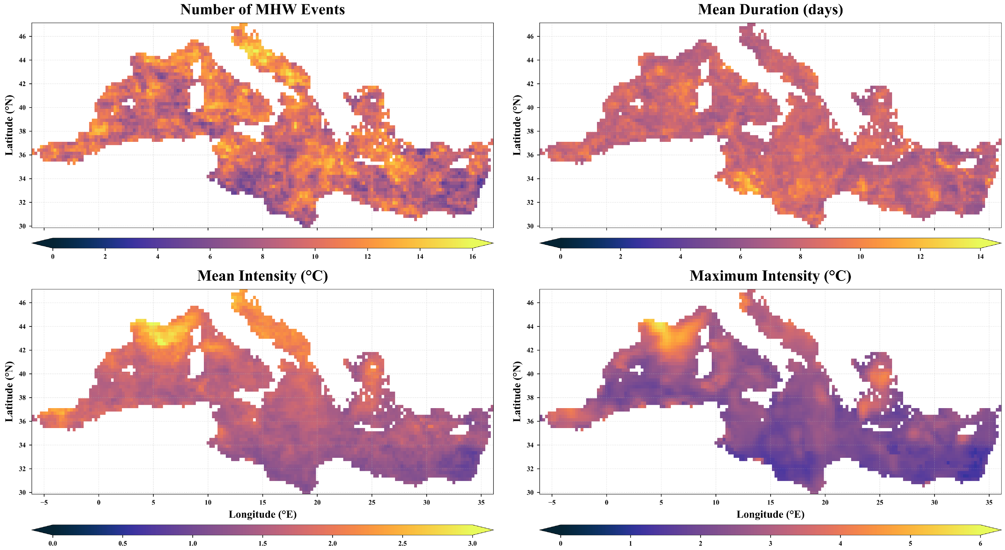
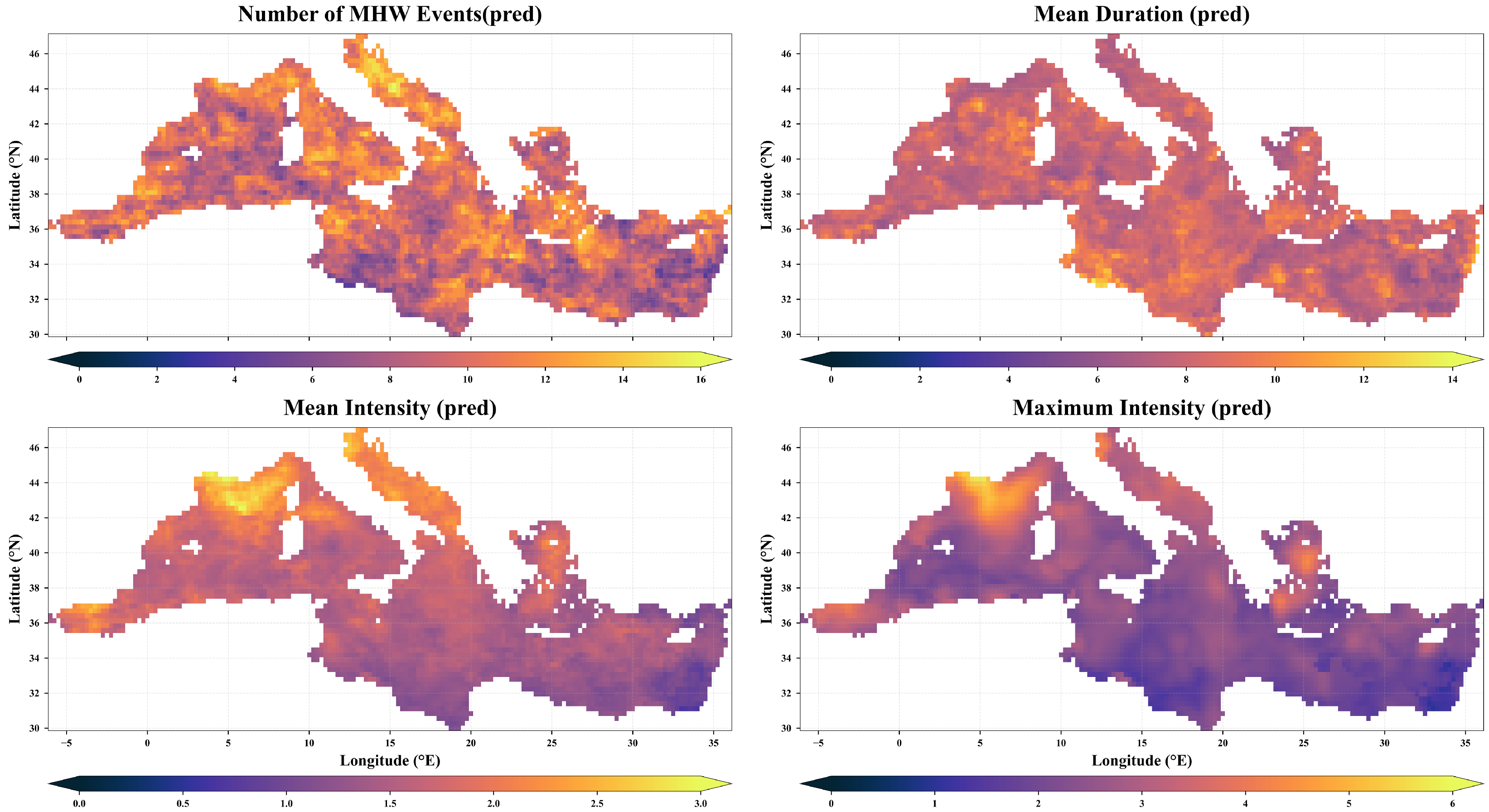
To evaluate the model’s capability in capturing marine heatwave characteristics, the predicted daily SST time series over the test period is post-processed using the MHW detection framework of [2]. A discrete MHW event is identified when the daily SST exceeds a seasonally varying 90th-percentile threshold for at least five consecutive days; events separated by a gap of two days or fewer are merged. The calendar-day threshold is computed by pooling SST values within an 11-day centred window (±5 days) over the climatological baseline period 1993–2010, and the resulting percentile curve is smoothed with a 31-day running mean. Four MHW metrics are derived from the detected events and used throughout Section 4 and Section 5: (i) annual frequency (number of discrete events per year), (ii) mean duration (days), (iii) mean intensity (°C, the event-averaged SST anomaly above the threshold), and (iv) cumulative intensity (°C·days yr⁻¹, the time-integrated anomaly above the threshold, normalised per year). The same detection procedure is applied identically to both the observed and predicted SST fields, so that all MHW maps presented in this study (see the MHW characteristic maps in Section 5) represent hindcast-reconstructed metrics diagnosed post hoc from the rolling one-day-ahead SST predictions, rather than direct multi-day MHW forecasts.

4. Materials and Methods

4.1. HW-OPINN Framework

Addressing the critical challenges faced by traditional Physics-Informed Neural Networks (PINNs) in marine heatwave prediction—including training instability, high parameter sensitivity, and static collocation point distribution—this study proposes a Heatwave-Optimized Physics-Informed Neural Network (HW-OPINN) framework. While maintaining physical consistency, this framework achieves significant improvements in prediction accuracy and training stability through three core innovative mechanisms.

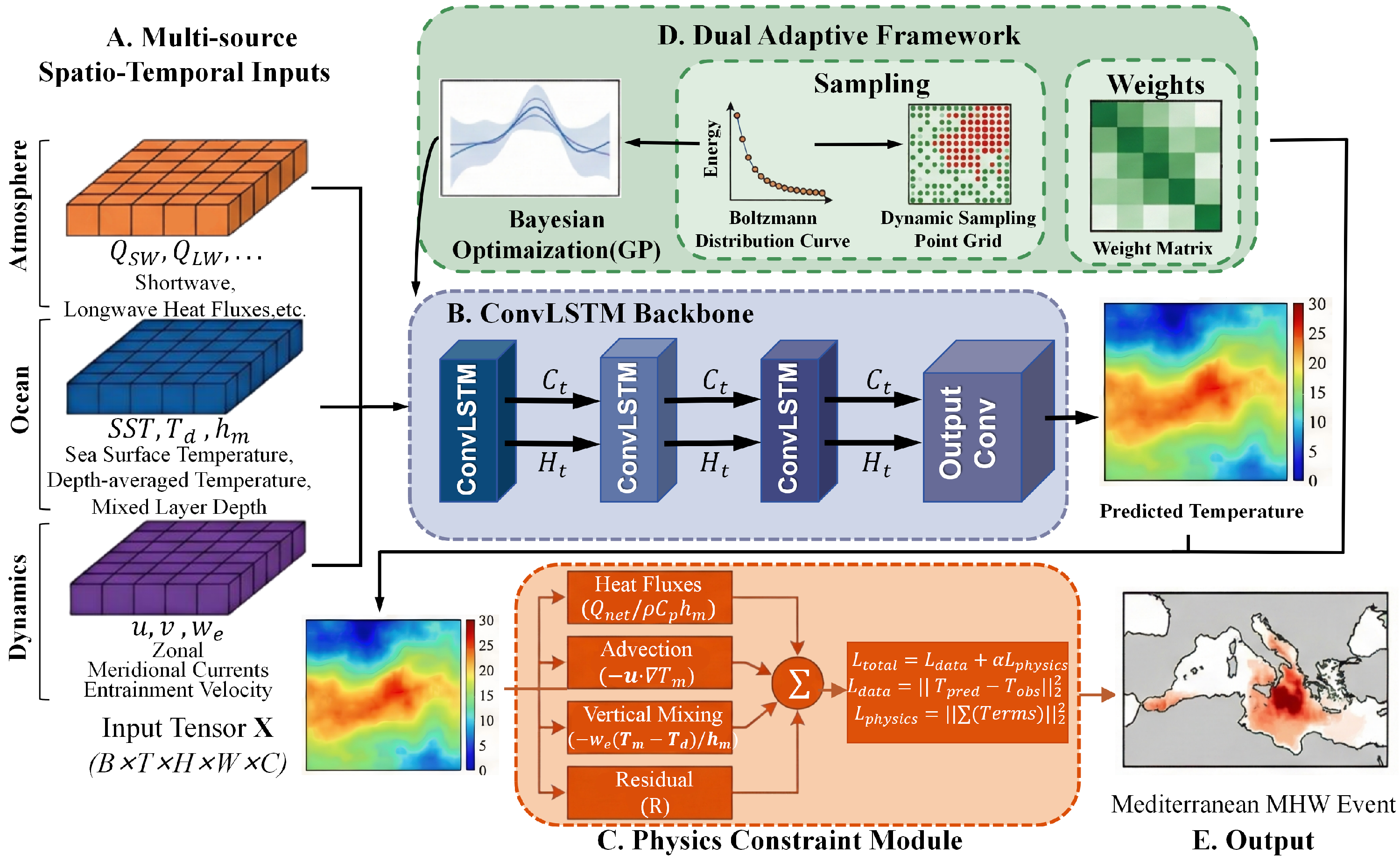
As illustrated in Figure 1, the HW-OPINN framework comprises five key components:

1.

Multi-source Spatio-temporal Input Construction (Panel A): Integrates ten physical channels—SST, shortwave and longwave radiation ($Q_{\mathrm{SW}}$, $Q_{\mathrm{LW}}$), surface latent and sensible heat fluxes (SLHF, SSHF), mixed-layer depth ($h_m$), zonal and meridional currents (u, v), entrainment velocity ($w_e$), and sub-mixed-layer temperature ($T_d$)—into a unified spatio-temporal tensor with a seven-day sliding window on a $0.{25}^{\circ }$ grid.

2.

ConvLSTM Prediction Backbone (Panel B): A three-layer ConvLSTM network with 64 hidden channels and $3\times 3$ kernels extracts spatio-temporal features from the input tensor. A $1\times 1$ convolution projects the final hidden state to a single-channel next-day SST prediction. No dropout, batch normalisation, or skip connections are used (see Section 4.4 and

Table 2. HW-OPINN ConvLSTM backbone architecture specification.

Layer	Output Channels	Kernel Size	Activation
ConvLSTM-1	64	$3\times 3$	Tanh
ConvLSTM-2	64	$3\times 3$	Tanh
ConvLSTM-3	64	$3\times 3$	Tanh
$1\times 1$ Conv	1	$1\times 1$	–

for full specification).

3.

Physical Constraint Modeling Module (Panel C): Constructs physical constraints based on the mixed-layer heat budget equation, embedding critical physical processes including air-sea interface heat flux, horizontal advection, and vertical mixing into the neural network training process.

4.

Dual Adaptive Framework (Panel D): Comprises three tightly coupled components: (i) a Bayesian optimisation module that uses Gaussian-process surrogates and expected-improvement acquisition to systematically search for optimal hyperparameters; (ii) an adaptive sampling module that dynamically redistributes physical collocation points via Boltzmann-distribution weighting, concentrating samples in high-gradient regions; and (iii) an adaptive weight-update module that adjusts region-specific physics-loss contributions through trainable weight coefficients and masking functions.

5.

Predicted SST Field (Panel E): The model outputs a daily SST forecast over the Mediterranean domain, which is subsequently used for marine heatwave identification and intensity analysis. The total training objective fuses the data-driven MSE loss with the physics-constraint loss, ensuring both prediction accuracy and physical consistency (see Section 4.5).

These modules work synergistically to constitute the complete optimization framework of HW-OPINN. The framework employs a hierarchical optimization strategy: the adaptive sampling module dynamically adjusts physical collocation point distribution based on historical loss patterns, the weight update module adjusts constraint strength across different regions in real-time, and the Bayesian optimization module systematically searches for globally optimal hyperparameters. All components work coordinately during training to jointly enhance the model’s prediction accuracy and training stability.

4.1.1. Physical Mechanisms and Governing Equations

The spatiotemporal evolution of mixed-layer temperature $T_m$, which serves as a widely used proxy for sea surface temperature in the upper ocean where wind-driven mixing produces nearly uniform temperature profiles, is governed by the mixed-layer heat budget equation [54,55]. This formulation is standard in MHW attribution studies [13,56] and provides the physical basis for the physics loss in HW-OPINN:

$${\displaystyle \frac{\partial T_m}{\partial t}}={\displaystyle \frac{Q}{\rho C_p{h}_m}}-\overrightarrow{u}·\nabla T_m-w_e{\displaystyle \frac{(T_m-T_d)}{h_m}}+R_{res}$$

(1)

where $T_m$ represents the mean mixed layer temperature; ${\displaystyle \frac{Q}{\rho C_p{h}_m}}$ denotes the surface net heat flux term, with Q being the net heat flux comprising net shortwave radiation $Q_{SW}$, net longwave radiation $Q_{LW}$, latent heat flux $Q_{LH}$, and sensible heat flux $Q_{SH}$; $\rho$ is seawater density; $C_p$ is the specific heat capacity of seawater; and $h_m$ represents the mixed layer depth.

The term $\overrightarrow{u}·\nabla T_m$ represents horizontal advection, where $\overrightarrow{u}=(u,v)$ is the horizontal ocean current velocity vector.

The term $w_e{\displaystyle \frac{(T_m-T_d)}{h_m}}$ represents vertical entrainment, where $w_e$ is the vertical ocean velocity, $T_d$ is the temperature at the mixed layer base, and $h_m$ is the mixed layer depth. $R_{res}$ represents residual terms that cannot be explicitly quantified.

Expanding Equation (1), the complete form of the heat budget equation becomes:

$$\begin{array}{cc}\hfill {\displaystyle \frac{\partial T_m}{\partial t}}& ={\displaystyle \frac{Q_{SW}+Q_{LW}-Q_{LH}-Q_{SH}}{\rho C_p{h}_m}}\hfill \\ \hfill & -u{\displaystyle \frac{\partial T_m}{\partial x}}-v{\displaystyle \frac{\partial T_m}{\partial y}}-w_e{\displaystyle \frac{(T_m-T_d)}{h_m}}+R_{res}\hfill \end{array}$$

(2)

4.1.2. Temperature Gradient Computation

Spatial gradients of $T_m$ in Equation (2) are computed using centred finite differences on the 0.25° grid. Because the study domain spans a wide latitude range (30.19°N–45.98°N), the zonal grid spacing is corrected for meridional convergence by a factor of $cos\left(\varphi \right)$, following standard spherical coordinate discretisation practice in geophysical fluid dynamics [57]. The full derivation of the curvature-corrected finite differences is provided in Appendix A.

It is important to clarify the physical assumptions underlying the use of the mixed-layer heat budget equation in this framework. The heat budget equation (Equation (2)) technically describes the evolution of depth-averaged mixed layer temperature ($T_m$), rather than the satellite-measured sea surface temperature (SST). However, using the mixed-layer heat budget as a physics constraint for SST prediction is a widely adopted approach in the field [39,41]. The rationale is that the mixed-layer heat budget captures the dominant thermodynamic processes—surface heat flux, horizontal advection, and vertical entrainment—that govern upper ocean temperature evolution.

Furthermore, this study employs daily-averaged NOAA OISST data as the prediction target. Daily averaging substantially reduces diurnal warm layer effects that cause the largest $T_m$–SST discrepancies, which primarily occur during daytime under calm, clear-sky conditions. For daily-averaged data, the mixed-layer heat budget provides a reasonable first-order physical constraint, while the neural network’s learning capacity compensates for residual discrepancies not captured by the simplified governing equation.

Regarding MHW detection, this approximation has minimal impact on MHW characterization. MHWs are defined based on SST exceeding climatological thresholds over sustained periods of at least five days [2]. Since MHW identification relies on daily or longer timescale SST anomalies rather than instantaneous skin temperature, the key MHW metrics—frequency, duration, and intensity—are derived from multi-day temperature evolution patterns that are well-captured by mixed-layer thermodynamics.

4.2. HW-OPINN (Heat Wave-Optimized Physics-Informed Neural Network)

Building upon recent advances in Physics-Informed Neural Networks (PINN), we propose an integrated framework that synergistically incorporates several state-of-the-art strategies for PINN optimization. This framework is applied, for the first time, to marine heatwave prediction, addressing complex oceanographic phenomena.

4.2.1. Physics-Informed Neural Networks (PINN)

Physics-Informed Neural Networks (PINN) provide a novel paradigm that combines physical constraints with data-driven learning. This approach not only captures patterns in observational data but, more importantly, can regularize and correct model predictions through physical constraints when data quality is insufficient or biased.

Specifically, to effectively embed the ocean mixed layer heat budget equation into model training, we construct a joint loss function comprising data loss and physics loss. The data loss component reflects the deviation between model predictions and observations, while the physics loss component measures whether model predictions satisfy the constraints imposed by the heat budget equation. This is formalized as follows:

$${\mathcal{L}}_{\mathrm{total}}={\lambda }_{\mathrm{data}}{\mathcal{L}}_{\mathrm{data}}+{\lambda }_{\mathrm{physics}}{\mathcal{L}}_{\mathrm{physics}}$$

(3)

$${\mathcal{L}}_{\mathrm{data}}={\displaystyle \frac{1}{N}}\sum _{i=1}^N{\left({\widehat{T}}_m^{\left(i\right)}-T_m^{\left(i\right)}\right)}^2$$

(4)

$${\mathcal{L}}_{\mathrm{physics}}={\displaystyle \frac{1}{M}}\sum _{j=1}^M{\left(\mathcal{R}(x_j,y_j,t_j)\right)}^2$$

(5)

where ${\lambda }_{\mathrm{data}}$ is the weight for data-driven loss (default value 1); ${\lambda }_{\mathrm{physics}}$ is the weight for physics loss, determining the relative importance of physical constraints; ${\mathcal{L}}_{\mathrm{data}}$ quantifies the deviation between model predictions and observations, with ${\widehat{T}}_m^{\left(i\right)}$ representing the model prediction for the i-th sample, $T_m^{\left(i\right)}$ denoting the true value for the i-th sample, and N indicating the number of samples used for data loss. ${\mathcal{L}}_{\mathrm{physics}}$ evaluates the degree to which model predictions satisfy the heat budget equation constraints, where M represents the number of samples used for physics loss, and $\mathcal{R}$ denotes the residual function of the governing equation.

Implementation Details

The physics residual is evaluated as follows. The temporal derivative is approximated using a forward finite difference between the network-predicted SST at time $t+1$ and the observed SST at time t, divided by $\Delta t=1$ day. This formulation directly couples the physics constraint to the prediction objective, ensuring that predicted temperature tendencies are consistent with the heat budget equation.

Spatial gradients are computed using centred finite differences with Earth-curvature corrections as described in Section 4.1.2. All other terms in the heat budget (Q, $h_m$, $\overrightarrow{u}$, $w_e$, $T_d$) are taken directly from the reanalysis input data at each collocation point.

The residual term $R_{\mathrm{res}}$ in Equation (2), representing unresolved sub-grid processes, is not explicitly modelled. Instead, the neural network implicitly absorbs these unresolved contributions through its learned representations. The physics loss thus serves as a soft constraint that guides predictions toward physical consistency without enforcing exact closure. The Bayesian-optimised weight $\alpha$ and the adaptive weighting mechanism jointly regulate the constraint strength, automatically relaxing it in regions where large residuals indicate substantial unresolved dynamics.

4.2.2. Adaptive Sampling Strategy

In traditional Physics-Informed neural networks, sampling points are typically uniformly distributed, and the model applies physics loss constraints to all data points (with physics sampling points M usually equal to data sampling points N). This approach has several deficiencies, as detailed in the Section 6. In constructing the HW-OPINN model, the adaptive sampling strategy is one of the key methods for improving model efficiency and accuracy. This strategy dynamically adjusts the spatial distribution characteristics of sampling points based on model performance during training. We innovatively introduce an intelligent sampling mechanism based on historical loss functions, continuously tracking the model’s physics prediction errors in different regions, optimizing sampling density in areas with dramatic gradient changes while appropriately reducing sampling frequency in regions with gentle field variations. The algorithm constructs a probability density distribution function by precisely quantifying local residuals, thereby providing scientific spatial guidance for newly generated sampling points.

Specifically, the theoretical foundation of the probability density distribution function originates from the Boltzmann distribution in statistical mechanics, which describes the energy distribution pattern in thermodynamic equilibrium systems. The Boltzmann distribution states that at a given temperature, the probability of a system being in a state with energy $E_i$ has an exponential relationship with that state’s energy, expressed as

$$P_i={\displaystyle \frac{e^{-E_i/\left(k_{B}T\right)}}{{\sum }_j{e}^{-E_j/\left(k_{B}T\right)}}}$$

(6)

where $P_i$ is the probability of the system being in energy state i, $k_B$ is the Boltzmann constant, and T represents the absolute temperature of the system. The exponential term in the numerator describes that the probability of individual energy state i occurring is negatively correlated with energy—higher energy states have lower occurrence probabilities. The summation term in the denominator, summing over all possible energy states, is called the partition function, ensuring that the sum of probabilities over all states equals 1. This formula reflects the system’s tendency toward energy distribution uniformization.

In practical applications, the probability density distribution function describes the probability of a random variable taking specific values or falling within certain intervals in a similar manner, reformulated as

$$p_i={\displaystyle \frac{e^{{\mathcal{L}}_{\mathrm{phys}}^{\left(i\right)}/T}}{{\sum }_{j=1}^M{e}^{{\mathcal{L}}_{\mathrm{phys}}^{\left(j\right)}/T}}}$$

(7)

where ${\mathcal{L}}_{\mathrm{phys}}^{\left(i\right)}$ represents the physics loss at a certain point. Unlike the standard Boltzmann distribution where the negative exponent favours low-energy states, here the sign is reversed so that points with higher physics residuals receive greater sampling probability. T is the temperature coefficient determining the concentration of the probability distribution: as $T\to \infty$, the distribution approaches uniform sampling, while as $T\to 0^{+}$, it concentrates on the highest-residual location. In this work, T is set to 1.0 (i.e., standard softmax), which provides a moderate balance between exploration and exploitation of high-residual regions.To ensure numerical stability when computing the exponentials, we subtract the maximum loss value before exponentiation:

$$p_i={\displaystyle \frac{e^{({\mathcal{L}}_{\mathrm{phys}}^{\left(i\right)}-{\mathcal{L}}_{\max })/T}}{{\sum }_{j=1}^M{e}^{({\mathcal{L}}_{\mathrm{phys}}^{\left(j\right)}-{\mathcal{L}}_{\max })/T}}}$$

(8)

where ${\mathcal{L}}_{\max }={max}_j{\mathcal{L}}_{\mathrm{phys}}^{\left(j\right)}$. This log-sum-exp trick prevents numerical overflow while preserving the relative probability distribution.

When T is high, more points are sampled uniformly; when T is low, the distribution becomes more concentrated on high-weight points, optimizing computational resources. The summation in the denominator is the cumulative exponential of scores for all possible events, serving a similar role to the denominator in the Boltzmann distribution.

The adaptive sampling strategy based on the Boltzmann distribution provides efficient spatial guidance for model training. Building on this foundation, we further introduce an adaptive weight update mechanism to enhance the model’s learning capability in important regions.

4.2.3. Adaptive Weight Update Mechanism

The weight coefficient update mechanism is one of the key strategies for improving model performance. This mechanism dynamically adjusts the weight distribution of physics constraint terms, achieving adaptive recognition and response to the importance of different regions. In traditional PINN, physics constraint terms typically employ uniform weight coefficients, a simple approach that ignores the complexity differences of physical processes across regions and fails to effectively capture dynamic characteristics in critical areas.

To overcome this limitation, we propose a residual-based adaptive weight update strategy. Specifically, this mechanism comprises the following core components: First, we introduce trainable weight coefficients $w_i$ for each sampling point, controlling their contribution to the physics loss through a mask function $\varphi (·)$:

$${\mathcal{L}}_{\mathrm{physics}}={\displaystyle \frac{1}{M}}\sum _{i=1}^M{w}_i·\varphi \left({\mathcal{R}}_i\right)·{\mathcal{R}}_i^2$$

(9)

where ${\mathcal{R}}_i$ is the corresponding physics residual at that point. The mask function must satisfy the property of monotonic increase to ensure that larger residuals correspond to larger weights. The mask function adopts a quadratic design:

$$\varphi \left({\mathcal{R}}_i\right)={\mathcal{R}}_i^2$$

(10)

This function possesses non-negativity and differentiability, providing smooth gradient information that effectively enhances training stability. Meanwhile, its concise form reduces computational overhead, facilitating improved training efficiency.

The weight coefficient update follows a gradient ascent strategy:

$$w_i^{(t+1)}=w_i^{\left(t\right)}+\alpha {\displaystyle \frac{\partial {\mathcal{L}}_{\mathrm{physics}}}{\partial w_i}}$$

(11)

where:

$${\displaystyle \frac{\partial {\mathcal{L}}_{\mathrm{physics}}}{\partial w_i}}={\displaystyle \frac{1}{M}}\varphi \left({\mathcal{R}}_i\right)·{\mathcal{R}}_i^2$$

(12)

To prevent runaway scaling and ensure training stability, the weights are clamped after each update:

$$w_i^{(t+1)}=\mathrm{clamp}\left(w_i^{(t+1)},w_{min},w_{max}\right)$$

(13)

where $w_{min}=0.1$ and $w_{max}=10.0$. This constraint ensures that no single collocation point dominates the physics loss while still allowing meaningful spatial differentiation. The weights are initialised to 1.0 and are not normalised, as absolute scaling is absorbed by the global physics weight.

The interaction between local adaptive weights $w_i$ and the global physics weight $\alpha$ follows a hierarchical structure. The total physics loss contribution to the training objective is $\alpha ·{\mathcal{L}}_{\mathrm{physics}}$, where ${\mathcal{L}}_{\mathrm{physics}}$ incorporates the local weights as defined in Equation (9). The global weight $\alpha$ (determined via Bayesian optimisation) controls the overall balance between data fitting and physics constraints, while the local weights $w_i$ modulate the relative importance across spatial regions. This design allows the model to maintain global physics-data balance while adaptively focusing on regions where constraints are poorly satisfied.

This gradient ascent mechanism ensures that weight coefficients evolve toward increasing physics loss, enabling the model to automatically intensify optimization efforts in high-residual regions during training. Through this approach, the model can adaptively allocate computational resources, focusing on regions where physics constraints are poorly satisfied, thereby improving overall prediction accuracy.

As for the update of neural network parameters, it still follows standard gradient descent optimization:

$${\theta }^{(t+1)}={\theta }^{\left(t\right)}-\eta {\displaystyle \frac{\partial {\mathcal{L}}_{\mathrm{total}}}{\partial \theta }}$$

(14)

This expression embodies the fundamental principle of parameter iteration, where ${\theta }^{(t+1)}$ represents the parameter values after the $(t+1)$-th iteration, ${\theta }^{\left(t\right)}$ denotes the parameters at the t-th iteration, $\eta$ is the learning rate controlling the step size of parameter updates, and ${\displaystyle \frac{\partial {\mathcal{L}}_{\mathrm{total}}}{\partial \theta }}$ represents the gradient of the total loss function with respect to network parameters.

4.3. Bayesian Optimization Framework

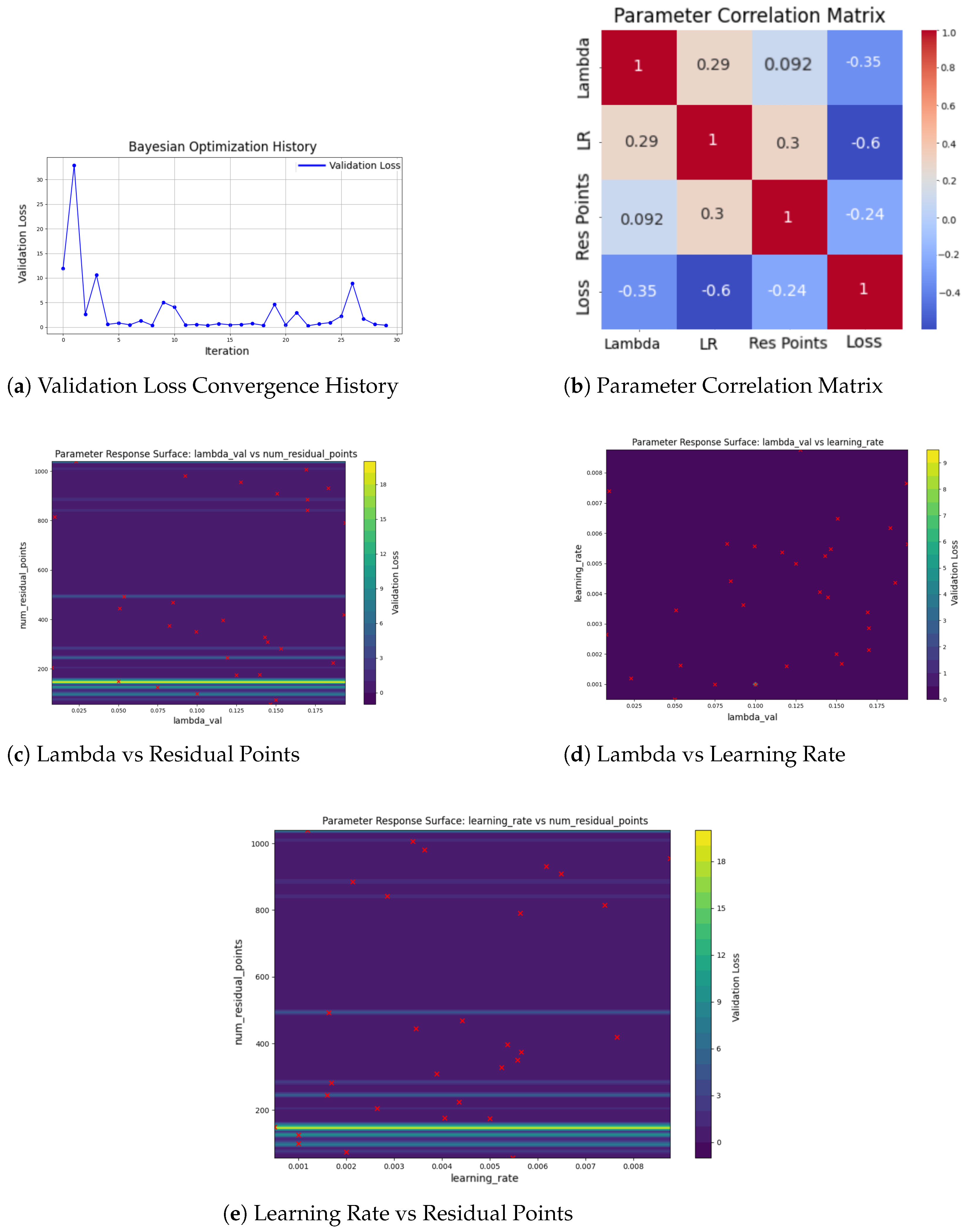
In practical applications of Physics-Informed Neural Networks (PINNs), the precise configuration of weights between physics constraints and data fitting terms significantly impacts model performance. This sensitivity stems from PINNs’ unique dual learning objectives: minimizing the difference between observed data and predicted values while ensuring satisfaction of given physical constraints such as partial differential equations. Previous research, including our work, demonstrates that these objectives maintain a delicate balance, where slight parameter adjustments can cause significant performance fluctuations.

Traditional parameter optimization methods, such as grid search or random search, often perform suboptimally when handling such highly nonlinear optimization problems. Therefore, we employ Bayesian Optimization (BO) to efficiently approach optimal solutions in this high-dimensional black-box optimization problem, automating the weight selection process.

The Bayesian optimization paradigm is an optimization methodology grounded in Bayesian theory. Its core principle involves constructing a probabilistic model of the relationship between parameters and performance based on historical observations, predicting the most promising parameter combinations to improve performance, and iteratively converging to optimal parameter sets.

Within our Bayesian optimization framework, we first establish a Gaussian Process (GP) surrogate model:

$$f\left(\theta \right)\sim \mathcal{GP}\left({\mu }_0\left(\theta \right),k(\theta ,{\theta }^{\prime })\right),$$

(15)

where $f\left(\theta \right)$ represents the objective function reflecting the performance of hyperparameter combinations; ${\mu }_0\left(\theta \right)$ serves as the prior mean function, providing initial estimates of hyperparameter performance; and $k(\theta ,{\theta }^{\prime })$ denotes the kernel function, capturing parameter correlations using a Radial Basis Function (RBF) kernel. Here, $\theta$ represents the current parameter point, and ${\theta }^{\prime }$ represents previously evaluated points. Given observed data $D={\left\{({\theta }_i,f\left({\theta }_i\right))\right\}}_{i=1}^n$, the GP can output a posterior distribution for any unevaluated point:

$${\mu }_n\left(\theta \right)={\mu }_0\left(\theta \right)+k(\theta ,\theta ){(K+{\sigma }^{2}I)}^{-1}(y-{\mu }_0\left(\theta \right)),$$

(16)

$${\sigma }_n^2\left(\theta \right)=k(\theta ,\theta )-k(\theta ,\theta ){(K+{\sigma }^{2}I)}^{-1}k(\theta ,\theta ),$$

(17)

where K represents the kernel matrix between observed points, I is the corresponding identity matrix, and ${\sigma }^2$ denotes the observation noise variance. The vector $k(\theta ,\theta )$ contains kernel function values between the prediction point and all observed points. The posterior distribution provides not only performance predictions ${\mu }_n\left(\theta \right)$ for unevaluated points but also quantifies prediction uncertainty through posterior variance ${\sigma }_n^2\left(\theta \right)$. The optimization process proceeds by maximizing the expected improvement:

$$EI\left(\theta \right)=({\mu }_n\left(\theta \right)-f\left({\theta }^{+}\right))\Phi \left(Z\right)+{\sigma }_n\left(\theta \right)\varphi \left(Z\right),$$

(18)

where $Z={\displaystyle \frac{{\mu }_n\left(\theta \right)-f\left({\theta }^{+}\right)}{{\sigma }_n\left(\theta \right)}}$, $f\left({\theta }^{+}\right)$ represents the current best observed value, and $\Phi (·)$ and $\varphi (·)$ are the cumulative distribution function and probability density function of the standard normal distribution, respectively. The parameter update rule selects the maximum expected improvement value.

Having established the theoretical foundations of Gaussian process-based Bayesian optimization for weight parameter tuning, we now present a comprehensive algorithm that systematically explores and optimizes the physics constraint weights in PINNs. The proposed algorithm synthesizes probabilistic surrogate modeling with sequential optimization strategies, implementing an iterative framework that progressively refines the weight configuration space. Through the integration of Gaussian process regression and expected improvement-based acquisition, our approach enables automated and efficient exploration of the parameter landscape while maintaining a careful balance between exploitation of promising regions and exploration of uncertain parameter spaces. The algorithm (Algorithm 1) encapsulates this methodology in a unified optimization procedure, providing a robust framework for determining optimal physics constraint weights that enhance PINN training stability and performance.

Algorithm 1 Bayesian Optimization for PINN Physics Weight Selection

Require: Parameter space $\Theta$, observed dataset $D={\left\{({\theta }_i,f\left({\theta }_i\right))\right\}}_{i=1}^n$, kernel function $k(\theta ,{\theta }^{\prime })$, convergence threshold $ϵ$, maximum iterations $T_{max}$ 1: Initialize GP prior mean ${\mu }_0\left(\theta \right)$ and observation noise variance ${\sigma }^2$ 2: Initialize best observed value $f\left({\theta }^{+}\right)\leftarrow {min}_{i}f\left({\theta }_i\right)$ 3: repeat 4:     Update GP posterior distribution using Equations (16) and (17) 5:     Calculate acquisition function value using Equation (18) 6:     Select next configuration: ${\theta }_{new}\leftarrow \underset{\theta \in \Theta }{argmax}EI\left(\theta \right)$ 7:     Evaluate PINN with ${\theta }_{new}$ and obtain $f\left({\theta }_{new}\right)$ 8:     Update observation dataset: $D\leftarrow D\cup \left\{({\theta }_{new},f\left({\theta }_{new}\right))\right\}$ 9:     Update best observed value: $f\left({\theta }^{+}\right)\leftarrow min(f\left({\theta }^{+}\right),f\left({\theta }_{new}\right))$ 10:   Check convergence: $\parallel f\left({\theta }_{new}\right)-f\left({\theta }^{+}\right)\parallel <ϵ$ or exceed $T_{max}$ 11: until converged 12: return Optimal weight configuration ${\theta }^{\ast }$ and corresponding performance $f\left({\theta }^{\ast }\right)$

Having established these key components of our framework—the temperature gradient computation, network architecture, adaptive sampling strategy, and adaptive weight update mechanism—we now present the complete HW-OPINN training algorithm (Algorithm 2). This algorithm synthesizes all previously described components into a unified training process, implementing both the physical constraint satisfaction and the adaptive mechanisms in a coherent framework.

Algorithm 2 HW-OPINN Training Algorithm

Require: training data features x, target y, sea-land mask m; initial learning rate $l_1$, physics weights $\lambda$; number of residual points $N_{residual}$; sampling update frequency $f_s$; mask function $M\left(\lambda \right)$ and its derivative $M^{\prime }\left(\lambda \right)$; maximum physics loss history length $L_{max}$; physics model function $f_{physics}\left(x\right)$ Ensure: Optimized model parameters 1: Initialization: 2:     Physics loss history: $L_{phys}\leftarrow \mathrm{zeros}(\mathrm{height},\mathrm{width},L_{max})$ 3:     Time step: $t\leftarrow 0$ 4:     Sampling probability: $p\leftarrow 1/(\mathrm{height}\times \mathrm{width})$ 5: repeat 6:     for each batch do 7:         Sample batch data $(x,y,m)$ 8:         Apply sea-land mask: $x_{valid}\leftarrow m\odot x$ 9:         Predict model output: $T_{pred}\leftarrow \mathrm{model}\left(x_{valid}\right)$ 10:       Calculate data loss: $L_{data}\leftarrow \mathrm{mean}\left[{(T_{pred}-y)}^2\right]$ 11:       Sample $N_{residual}$ indices $(i_k,j_k)$ with probabilities p 12:       Calculate physics predictions at sampled points $(i_k,j_k)$: $T_{physics,k}\leftarrow f_{physics}\left(x_{valid,k}\right)$ 13:       Compute physics loss using Equation (5) 14:       Update physics loss history: Store $L_{physics}$ into $L_{phys}[:,:,tmod{L}_{max}]$ 15:       if $tmod{f}_s=0$ then 16:           Calculate average historical physics loss: ${\overline{L}}_{phys,i,j}\leftarrow {\displaystyle \frac{1}{L_{max}}}{\sum }_{k=0}^{L_{max}-1}{L}_{phys,i,j,k}$ 17:           Update sampling probabilities using Equation (7) 18:       end if 19:       Calculate total loss using Equation (3) 20:       Update physics weights and model parameters using Equations (11) and (14) 21:       Increment time step: $t\leftarrow t+1$ 22:   end for 23: until converged

4.4. Network Architecture

The prediction backbone of HW-OPINN employs a three-layer ConvLSTM architecture. The input tensor $\mathbf{X}\in {\mathbb{R}}^{B\times 7\times 62\times 169\times 10}$ comprises a 7-day sliding window of 10 physical channels on a $0.{25}^{\circ }$ Mediterranean grid. The ten channels include sea surface temperature, radiation fluxes ($Q_{\mathrm{SW}}$, $Q_{\mathrm{LW}}$), surface heat fluxes (SLHF, SSHF), mixed-layer depth, horizontal currents (u, v), entrainment velocity, and sub-mixed-layer temperature.

Input features are normalised via LayerNorm before being processed by three stacked ConvLSTM cells (64 hidden channels, $3\times 3$ kernels). A $1\times 1$ convolution maps the final hidden state to a single-channel next-day SST prediction. The sole output target is SST; no auxiliary quantities are predicted.

4.5. Training Configuration

The model is trained by minimising the combined loss ${\mathcal{L}}_{\mathrm{total}}={\mathcal{L}}_{\mathrm{data}}+\alpha {\mathcal{L}}_{\mathrm{physics}}$, where ${\mathcal{L}}_{\mathrm{data}}$ is the MSE over ocean grid points and ${\mathcal{L}}_{\mathrm{physics}}$ is the heat-budget residual evaluated at adaptively sampled collocation points. The physics-loss weight $\alpha$ is determined through Bayesian optimisation (see

Table 3. Training configuration of HW-OPINN.

Hyperparameter	Value
Optimiser	Adam
LR schedule	ReduceLROnPlateau
Batch size	8–16
Early stopping	patience = 10
Physics weight $\alpha$	Bayesian-optimised
Regularisation	None (physics-constrained)

for full training configuration).

Training uses Adam optimiser with ReduceLROnPlateau scheduling. The batch size ranges from 8 to 16 depending on available GPU memory. Early stopping (patience = 10) is applied to prevent overfitting. No dropout, weight decay, or batch normalisation is used, as the physics constraint provides implicit regularisation. All experiments are conducted on NVIDIA A100 GPUs using PyTorch 2.0.1.

5. Experiments

5.1. Experimental Results and Analysis

5.1.1. Sea Surface Temperature Prediction Performance

To rigorously evaluate the contribution of each proposed component, we compare four model configurations that share the identical ConvLSTM backbone (Table 2) and differ only in their training strategy, as summarised in

Table 4. Comparison of model configurations on the test set. All models share the identical ConvLSTM backbone (Table 2) and differ only in training strategy. All metrics are evaluated at a one-day forecast lead time (7-day input window) over the 2015–2018 test period.

Model Configuration	Test MSE	Test MAE	Test RMSE	Test RMSE (Norm.)
ConvLSTM (data-only)	0.016275	0.092775	0.127575	0.005037
Standard PINN ($\alpha =0.1$)	0.016550	0.092600	0.128661	0.005079
HW-OPINN ($\alpha =0.087$)	0.009138	0.054154	0.095595	0.003767
HW-OPINN ($\alpha =0.1$)	0.012624	0.070986	0.112358	0.004436

.

The first configuration, ConvLSTM (data-only), is trained with only the MSE data loss and serves as the primary baseline. The second, Standard PINN, adds the heat-budget physics loss with a manually set weight of $\alpha =0.1$ but uses static uniform sampling and uniform collocation-point weights, representing a conventional PINN without adaptive mechanisms. The third, HW-OPINN with $\alpha =0.087$, is the full proposed framework incorporating adaptive sampling, adaptive weighting, and Bayesian-optimised physics weight. The fourth, HW-OPINN with $\alpha =0.1$, retains adaptive sampling and weighting but uses a manually fixed physics weight, serving as an ablation to isolate the contribution of Bayesian weight tuning.

Compared with the ConvLSTM baseline, HW-OPINN with $\alpha =0.087$ achieves relative improvements of 43.9% in MSE, 41.6% in MAE, and 25.1% in RMSE. Compared with the Standard PINN, the corresponding improvements are 44.8%, 41.5%, and 25.7%, respectively. These gains are attributable entirely to the proposed adaptive training mechanisms, as all configurations share an identical network architecture.

Comparing the two HW-OPINN variants further demonstrates the benefit of Bayesian weight optimisation: the Bayesian-tuned weight yields a 27.6% MSE reduction over manual weight selection within the same adaptive framework, confirming that systematic hyperparameter tuning provides meaningful gains beyond the adaptive sampling and weighting mechanisms alone.

5.1.2. Sensitivity Analysis of PINN Performance to Physical Constraints

The effectiveness of Physics-Informed Neural Networks (PINNs) heavily depends on how well they balance data-driven learning with physical constraint satisfaction. This section presents a comprehensive analysis of PINN sensitivity to various physical constraint configurations, examining both the impact of constraint weights and sampling point distribution.

Impact of Physical Constraint Weights

The weighting coefficient ($\lambda$) of physical constraints plays a crucial role in determining the balance between data fitting and physical law adherence. Our investigation reveals that this relationship is notably non-linear and exhibits distinct behavioral regimes across different weight magnitudes.

We conducted a systematic comparison between traditional PINNs and the proposed heat wave-optimized Physics-Informed neural network (HW-OPINN) across various $\lambda$ values. The analysis encompasses multiple performance metrics including prediction accuracy (RMSE), physical constraint satisfaction (residual error), and computational efficiency (inference time).

Our findings indicate that while increased physical constraint weights generally improve physical consistency, there exists a critical threshold beyond which additional weight increases yield diminishing returns and may even deteriorate overall performance. This behavior can be attributed to the competing objectives in the loss function and the inherent numerical challenges in optimization.

Influence of Constraint Sampling Configuration

The spatial distribution and density of points where physical constraints are evaluated significantly impact both the learning dynamics and final performance of PINNs. We conducted a systematic investigation of various sampling strategies and their effects on model convergence and accuracy.

Our analysis of different sampling configurations across various physical constraint weights reveals several key findings:

1.

Adaptive sampling strategies consistently outperform uniform sampling, particularly in regions with high physical gradient variations.

2.

The optimal number of sampling points exhibits a non-linear relationship with the physical constraint weight, suggesting the existence of an efficient frontier in the sampling-weight space.

3.

The computational overhead of increased sampling density must be balanced against the marginal improvements in physical constraint satisfaction.

These results provide practical guidelines for implementing PINNs in real-world applications, where both accuracy and computational efficiency are critical considerations. Furthermore, they suggest that the traditional approach of uniform sampling may be suboptimal for complex physical systems with varying scales of behavior.

5.1.3. Marine Heatwave Characteristics and Spatial Distribution Analysis

Building upon accurate SST predictions, we evaluated HW-OPINN’s capability in forecasting marine heatwave (MHW) characteristics. Figure 2 and Figure 3 present the observed and predicted spatial distributions of four key MHW metrics across the Mediterranean Sea during 2015–2018, demonstrating the model’s exceptional performance in capturing MHW features. Analysis of Mediterranean MHWs revealed two distinct regional patterns:

Western Pattern

The western Mediterranean (particularly the Ligurian and Tyrrhenian Seas) and the Adriatic Sea exhibited high-frequency occurrence zones. These regions demonstrated frequent MHW events with high mean and maximum intensities, albeit with relatively shorter average durations, indicating intense but brief heatwave episodes.

Eastern and Southern Pattern

The eastern and southern Mediterranean (including waters south of Sicily) displayed lower event frequencies but extended event durations. This characteristic was particularly prominent in waters south of Crete and Sicily, potentially attributable to stable water mass structures and reduced vertical mixing processes.

HW-OPINN successfully captured the key features of both regional patterns, exhibiting particular accuracy in intensity predictions and spatial gradient representations. However, minor prediction biases were observed in specific regions, such as slight overestimation of MHW frequency along the central Adriatic coast and discrepancies in predictions around Sicily and Sardinia. These localized biases primarily stem from inherent limitations in neural network processing of rapid temperature field variations near boundary regions. Nevertheless, the model effectively characterized the spatiotemporal distribution of Mediterranean MHWs, providing reliable scientific basis for understanding regional heatwave evolution patterns.

Quantitative Comparison of MHW Detection Performance

To provide a rigorous quantitative assessment of MHW prediction capabilities, we computed detection metrics following the definition of [2].

Table 5. Comparison of Marine Heatwave Detection Metrics (Test Period: 2015–2018). MHW events were diagnosed post hoc from rolling one-day-ahead SST predictions following [2], with the 90th-percentile threshold computed over the climatological baseline period (1993–2010) and a minimum duration of five consecutive days (see Section 3 for full criteria). Values represent spatially-averaged Mean Absolute Error (MAE). Bold indicates best performance.

Method	Frequency (events/year)	Duration (days)	Mean Intensity (°C)	Cumulative Intensity (°C·days/year)
ConvLSTM	0.844	4.032	0.102	21.83
Standard PINN	0.839	4.318	0.117	29.60
HW-OPINN	0.822	3.999	0.111	25.82

presents the Mean Absolute Error (MAE) comparison across all methods. HW-OPINN achieves the lowest MAE for event frequency (0.822 events/year) and duration (3.999 days), representing improvements of 2.7% and 0.8% over ConvLSTM, respectively. These metrics are particularly important for operational MHW early warning, as accurate prediction of event occurrence and persistence directly supports decision-making in marine ecosystem management. For intensity-related metrics, all methods achieve comparable performance, with differences within 0.02 °C for mean intensity, suggesting that the physics constraints in HW-OPINN primarily enhance the temporal prediction of MHW events.

5.1.4. Bayesian Optimal Weight Search Results

This investigation presents a systematic analysis of a Bayesian optimization-based approach for neural network hyperparameter tuning. The method simultaneously optimizes three critical hyperparameters: regularization coefficient (lambda), learning rate, and the number of residual points.

The optimization history curve (Figure 4a) reveals distinctive convergence characteristics. Initial iterations exhibit substantial validation loss fluctuations, with peaks approaching 30, reflecting the algorithm’s exploratory phase in the parameter space. Subsequently, the validation loss demonstrates a stable descent, converging below 1 after the 15th iteration, indicating successful identification of optimal parameter combinations.

In the optimization process of Physics-Informed Neural Networks (PINNs), we observed an intriguing phenomenon: the intricate interplay between physical constraint strength ($\lambda$), sampling point density, and total loss. The correlation matrix (Figure 4b) quantifies these relationships, offering novel insights into PINN optimization dynamics.

Notably, the physical constraint coefficient $\lambda$ exhibits a −0.35 negative correlation with total loss. This moderate negative correlation reveals a key insight: while increased physical constraint weights guide the neural network toward more physically consistent solutions, this influence is distinctly nonlinear. This finding challenges the conventional intuition that stronger physical constraints invariably yield superior results.

The significant negative correlation (−0.6) between learning rate (LR) and total loss illuminates another crucial aspect of optimization dynamics. This indicates that optimizer behavior remains substantially governed by learning rate modulation, even in the presence of physical constraints. This observation emphasizes the critical balance between numerical optimization and physical constraints in PINN training.

The relatively weak correlation (−0.24) between residual points and validation loss, while seemingly trivial, carries profound implications. It suggests that merely increasing the sampling points for physical residual computation does not necessarily lead to improved performance, corroborating findings from related work by Bonfanti et al. [53].

Of particular interest is the 0.29 positive correlation between $\lambda$ and learning rate. This positive association suggests a potential “compensation mechanism”: as physical constraints strengthen, the optimization algorithm tends to adopt higher learning rates to maintain effective parameter updates. This insight provides new directions for designing adaptive optimization strategies.

The response surface visualizations (Figure 4c–e) further illustrate the complex parameter interactions. Figure 4c demonstrates that validation loss remains relatively stable across different lambda values when residual points are kept at lower ranges (below 200), but exhibits increased sensitivity at higher residual point counts. Figure 4d reveals a relatively smooth loss landscape in the lambda-learning rate space, with optimal performance achieved at moderate values of both parameters. Figure 4e shows similar patterns for learning rate versus residual points, confirming that the number of residual points has limited impact on model performance when other hyperparameters are appropriately configured.

These observations not only deepen our understanding of PINN optimization dynamics but also provide quantitative foundations for designing more efficient training strategies. Specifically, they underscore the necessity of considering physical constraint strength, optimization dynamics, and computational efficiency as three key dimensions in PINN design. Our findings demonstrate that successful PINN optimization requires a delicate balance among these competing objectives. These insights not only directly inform PINN development but also offer valuable perspectives for applying deep learning to broader scientific computing challenges.

6. Discussion

6.1. Analysis of Traditional PINNs’ Failure Mechanisms

Physics-Informed Neural Networks (PINNs) have garnered significant attention as a deep learning methodology that integrates physical knowledge. Their core advantage lies in the fusion of data-driven approaches with physical laws, enabling reliable predictions under scenarios of data scarcity or noise contamination. Theoretically, the proposed HW-OPINN framework incorporates the mixed-layer heat budget equation as a physical constraint within its loss function, leveraging both limited observational data and oceanographic thermodynamic principles to provide prior information for Mediterranean marine heatwave prediction. While PINNs in general can embed various governing equations as physical constraints, the specific formulation adopted here is tailored to the ocean mixed-layer thermodynamics relevant to MHW genesis. However, empirical evidence suggests that PINNs have not demonstrated their anticipated advantages, occasionally underperforming traditional data-driven methods in both accuracy and convergence rate, necessitating a thorough analysis of these performance discrepancies.

From an optimization theory perspective, the inefficacy of PINNs largely stems from the complexity of their loss function landscape. The incorporation of the mixed-layer heat budget equation as a constraint term in the loss function constructs an extraordinarily complex optimization objective. This equation encompasses multiple physical processes, including horizontal advection, vertical mixing, and net heat flux terms. The derivatives obtained through automatic differentiation not only increase computational instability but, more critically, render the loss function landscape exceptionally rugged with numerous local minima. Traditional optimization algorithms are prone to becoming trapped in local optima when handling such nonlinear physical systems. Moreover, the complexity of parameter gradients in computing high-order derivatives and satisfying PDE residuals frequently leads to gradient vanishing or exploding problems in the optimization space.

The Mediterranean Sea, as a semi-enclosed basin, exhibits significant spatiotemporal variability in its mixed-layer temperature field. Under the combined influence of atmospheric forcing, Atlantic water inflow through the Strait of Gibraltar, and complex topography, different marine regions display distinct temperature evolution characteristics. Particularly during summer, intense solar radiation elevates surface water temperatures, establishing pronounced vertical density gradients. This stratification phenomenon inhibits vertical mixing, making net heat flux and horizontal advection the dominant processes. Conversely, in winter, strong atmospheric cooling and wind-induced mixing disrupt stratification, enhancing vertical mixing effects. More significantly, recent frequent marine heatwaves have induced dramatic temperature elevations in certain critical regions, altering conventional temperature distribution patterns. These complex physical characteristics pose formidable challenges for PINNs implementation.

In conventional PINNs, the model applies uniform weights to all physical constraint points within the computational domain, a “one-size-fits-all” approach with significant limitations. Firstly, different regions exhibit fundamentally varying levels of physical complexity. For instance, coastal and strong convection zones in the Mediterranean demonstrate substantially more complex temperature field behavior than open waters, requiring additional computational resources for accurate representation. However, traditional PINNs employ identical optimization weights for these regions and simpler areas, resulting in insufficient prediction accuracy in critical zones. Secondly, during training, different constraint points often converge at varying rates. While some regions may achieve satisfactory prediction performance early in the process, complex areas require extended optimization periods. The traditional approach maintains identical optimization intensity for well-converged points, resulting in computational resource inefficiency. Thirdly, temperature field gradient distributions typically exhibit high heterogeneity, particularly during heatwaves, with certain regions potentially experiencing dramatic temperature gradients. These gradient transition zones require more refined optimization to accurately describe rapid temperature variations, while gradient-gentle regions can achieve adequate precision with lower optimization weights.

In practical applications, these challenges interweave with data quality issues and physical model uncertainties. When observational data exhibits excessive noise or uneven distribution, PINNs must simultaneously satisfy both data and physical constraints. Unstable data signals may counteract beneficial priors from physical equations, making it difficult for the network to find an equilibrium point. Furthermore, the residual terms in the mixed-layer heat budget equation represent heat budget processes that are challenging to quantify directly. These processes may be crucial in actual oceanic systems but are oversimplified in the equation. This “signal conflict” between data and physical equations often leads to opposing optimization objectives.

In this context, PINNs effectively serve more as a specialized regularization mechanism. While traditional regularization constrains model complexity through $L_1$ and $L_2$ norms, PINNs employ mixed-layer heat budget equation residuals as constraints, attempting to restrict the neural network’s solution space within physically plausible bounds. Although this physics-based regularization has clear physical significance in theory and does constrain the model’s solution space to some extent, its primary function is not to directly enhance model prediction accuracy but rather to improve physical consistency and generalization capability through physical constraints. When dealing with complex oceanic systems, physical equation constraints may fail to comprehensively capture various nonlinear interactions and small-scale processes in the actual system. Consequently, PINNs in practice must find an appropriate balance between physical constraints and data fitting, a balance that does not always significantly improve model accuracy like traditional optimization methods.

Beyond these limitations, traditional PINNs models lack dynamic adjustment capabilities, unable to dynamically modify regional weights or importance based on training feedback. This “static” approach prevents the model from effectively responding to rapid temperature field changes during heatwaves or adjusting optimization strategies based on training performance at different stages. Particularly during recent frequent marine heatwave events, different regions respond distinctly to extreme temperature increases, and uniform weighting strategies struggle to accurately capture temperature evolution characteristics in key regions.

In conclusion, while PINNs theoretically provide a robust framework integrating physical knowledge with data-driven methods, the Mediterranean marine heatwave prediction case vividly reveals fundamental challenges PINNs face in handling complex physical systems. This example demonstrates that relying solely on simplified physical constraints may be insufficient to effectively guide deep learning model training, particularly when confronting environments with significant spatiotemporal variability and complex dynamic characteristics like the Mediterranean Sea.

6.2. Advantages of HW-OPINN

Based on the identified limitations of traditional PINNs, HW-OPINN’s advantages manifest primarily through its dynamic adaptation capabilities. Where traditional PINNs struggle with uniform weighting across regions of varying complexity, HW-OPINN intelligently distributes computational resources based on the actual physical complexity and convergence needs of different Mediterranean Sea regions. The model’s adaptive weight mechanism efficiently handles the disparate convergence rates across regions, redirecting computational focus as needed rather than maintaining fixed optimization intensities. Additionally, through Bayesian optimization, HW-OPINN effectively resolves the fundamental tension between physical constraints and observational data fitting that traditionally undermines PINNs’ performance. This balanced approach proves particularly valuable for capturing the complex temperature dynamics during marine heatwave events, where traditional static approaches often fail.

6.3. Limitations and Future Directions

Several limitations of this study should be acknowledged. First, the mixed-layer heat budget equation used as the physics constraint describes the evolution of depth-averaged mixed layer temperature ($T_m$) rather than sea surface temperature (SST). While this approximation is reasonable for daily-averaged data where diurnal variability is minimized, and has minimal impact on MHW detection which operates on multi-day timescales, systematic differences between $T_m$ and instantaneous SST can occur under stratified conditions. Future work could explore surface-specific physical formulations or explicit $T_m$–SST correction schemes to further improve physical consistency.

Second, the framework relies on reanalysis data products (CMEMS, ERA5, OMEGA3D) as input features. These products incorporate assimilated observational information, providing high-quality inputs for model development and validation. However, this limits direct applicability to operational real-time MHW forecasting, where reanalysis products are unavailable for future time steps. This characteristic is common to reanalysis-based MHW studies [13,56], which focus on mechanistic understanding, MHW attribution analysis, and methodological validation rather than operational prediction.

In particular, the vertical velocity at the mixed-layer base is diagnosed from the OMEGA3D product, which relies on a quasi-geostrophic assumption that may underestimate ageostrophic contributions such as submesoscale frontal circulations and wind-driven Ekman pumping. Incorporating explicitly resolved vertical velocity fields from high-resolution ocean models would help quantify the sensitivity of the physics constraint to this approximation and represents an important direction for future investigation.

Extension to operational MHW early warning systems would require: (1) coupling with numerical ocean forecast systems (e.g., CMEMS forecast products) to provide predicted forcing fields with appropriate lead times; (2) incorporating uncertainty quantification for forecast-derived inputs to provide probabilistic MHW predictions; or (3) developing ensemble approaches that account for input uncertainty and provide confidence intervals for MHW onset timing and intensity. These represent important future research directions toward operational MHW prediction capabilities.

Despite these limitations, this study demonstrates that Physics-Informed constraints combined with adaptive optimization strategies can significantly improve SST prediction accuracy compared to purely data-driven approaches, which subsequently enhances the fidelity of downstream MHW detection. The framework establishes a methodological foundation for future development toward operational MHW early warning applications.

7. Conclusions

This study proposes a Heat Wave-Optimized Physics-Informed Neural Network (HW-OPINN) framework that synergistically integrates ocean mixed-layer heat budget dynamics with adaptive deep learning techniques for marine heatwave prediction. Validated in the Mediterranean Sea using multi-source reanalysis data spanning 1993–2018, HW-OPINN achieves a test mean squared error of 0.009138 and root mean squared error of 0.095595 °C, representing improvements of 43.9% and 25.1%, respectively, compared to the ConvLSTM baseline, and 44.8% and 25.7% over standard PINN. The model successfully reproduces key marine heatwave characteristics, achieving the lowest mean absolute error for event frequency (0.822 events/year) and mean duration (3.999 days) among all compared methods, while accurately capturing the spatial heterogeneity of heatwave intensity distributions.

The framework addresses fundamental challenges in physics-informed neural networks through three key innovations. First, an adaptive sampling strategy based on Boltzmann distribution dynamically reallocates physical collocation points toward high-gradient regions, enabling efficient capture of rapid temperature variations during heatwave evolution. Second, a residual-based adaptive weight update mechanism automatically modulates physical constraint contributions across spatially heterogeneous regions, allowing the model to focus computational resources where physics constraints are poorly satisfied. Third, a Bayesian optimization framework employing Gaussian process surrogates systematically balances physical constraints against data fitting objectives, effectively mitigating the training instability and excessive parameter sensitivity inherent in traditional PINNs.

Several limitations warrant acknowledgment. The mixed-layer heat budget equation used as the physics constraint describes depth-averaged mixed layer temperature rather than instantaneous sea surface temperature, which may introduce systematic differences under stratified conditions. The framework’s reliance on reanalysis data products limits direct applicability to operational real-time marine heatwave forecasting where such products are unavailable for future time steps. Future work should explore surface-specific physical formulations to improve consistency between mixed-layer and sea surface temperature predictions, incorporate explicitly resolved vertical velocity fields from high-resolution ocean models, develop probabilistic frameworks for uncertainty quantification in operational forecasting systems, and extend the methodology to other ocean basins to assess generalization capabilities.

In conclusion, this study demonstrates that carefully designed physics-informed neural networks can effectively combine the interpretability of physical models with the pattern recognition capabilities of deep learning, providing a promising pathway toward reliable prediction of extreme ocean events in support of climate adaptation and marine resource management. The proposed HW-OPINN framework offers both theoretical insights and practical guidance for advancing Physics-Informed machine learning methodologies in Earth system sciences.