Reconstructing Horizontal Displacement Through Deep Learning in Multiple-Pairwise Satellite Image Correlation

Highlights

What are the main findings?

• A deep-learning autoencoder is trained to remove Sentinel-2 correlated noise, enabling the recovery of clean displacement signals from any multiple-pairwise satellite image correlation (MPIC).
• The autoencoder can effectively remove correlated noises in the input MPICs, and accurately reconstruct denoised surface displacement in synthetic and real datasets.

What are the implications of the main findings?

• The method enables robust, automatic displacement extraction without manual intervention or prior knowledge of fault kinematics, improving the usability and accuracy of optical image correlation.
• The approach shows broad potential for reconstructing high-quality horizontal displacements across various tectonic and geomorphological processes, including earthquake ruptures, glacier flow, dune migration, and slow-moving landslides.

Abstract

High-resolution satellite images are frequently used to measure horizontal displacements caused by earthquakes, providing valuable insights into rupture behaviors and mechanical properties of seismogenic faults. The displacement of interest, however, is often contaminated by correlated noises. Therefore, accurate separation of the displacement from noise is crucial to improve the quality of the deformation map. In this study, we used a deep-learning autoencoder to eliminate noise and reconstruct clean displacement in multiple-pairwise satellite image correlation (MPIC). To achieve the desired denoising performance, the autoencoder was initially trained and validated on the MPIC synthetic datasets with simulated noises and noises from Sentinel-2 images, respectively. The experimental results indicate that our autoencoder successfully recovered denoised displacement signals in the input MPICs under various noise conditions. Upon applying the autoencoder to the actual MPICs over the 2021 Maduo earthquake, the denoised displacements were successfully reconstructed, showcasing its capability to real MPIC data. A higher consistency between the autoencoder’s reconstruction and GPS- and InSAR-based displacements demonstrated that our encoder outperforms both traditional denoising methods and the autoencoder trained on synthetic data. Moreover, the autoencoder can also recover the clean surface signal associated with a dune migration near the Maduo rupture, revealing a previously unreported migrating feature. Overall, the autoencoder exhibits potential in reconstructing high-quality horizontal displacements related to a range of tectonic and geomorphological processes.

1. Introduction

Horizontal displacement near earthquake ruptures provides valuable observations to study the rupture behaviors and mechanical properties of seismogenic faults [1,2,3,4,5]. It is challenging, however, to directly measure fine displacement in near-fault areas using common geodetic measurements, such as Interferometric Synthetic Aperture Radar (InSAR) and Global Navigation Satellite System (GNSS) [6,7]. The challenge lies in either the general decorrelation of SAR interferometry due to large-amplitude ground motions or the unavailability of dense displacements due to sparse continuous GNSS stations. Alternatively, the subpixel correlation technique can be applied to satellite optical images to detect the horizontal displacements [8,9,10,11,12]. However, the corruption or even concealment of the displacement signals by correlated noises can result in false detection or biased measurements.

The correlated noise often arises due to rotational and translational shifts resulting from orbital and ortho-rectification errors, stripe artifacts of embedded pushbroom sensors, satellite jitter undulation, and topographic artifacts [13,14,15,16]. Several techniques have been proposed to correct these correlated noises, such as deramping and destriping in the along-track and across-track directions, filtering geometry artifacts, and modeling digital elevation model errors [7,17,18,19,20,21]. After applying the aforementioned corrections, however, it is quite often that there are still residual errors in the data. The remaining errors, together with unknown image distortions and random image noises derived from thermomechanical and electronic effects, could still contaminate the displacement signals [14,22,23]. In addition, the presence of illumination intensity changes (e.g., low contrast, blurring, and different positions of the light source), apparent movement caused by specular reflectance features, and strong soil surface state changes can also amplify the correlated noises [18]. Therefore, it is crucial to develop new methods to more accurately separate displacement signals from the correlated noises.

Recently, several MPIC denoising methods, such as temporal filtering or stacking, have been applied to suppress correlated noises and improve displacement detection [4,7,11,16]. These methods assume that the displacement signals are more coherent in space and time than the noises, typically applying a low-pass filter or stacking to suppress the noises. However, insufficient filtering can still leave significant noise in the data, or excessive filtering may alter the target displacement. Additionally, these methods cannot isolate noise from the low-amplitude displacement signals due to their inability to extract local nonlinear features. Thus, a more effective processing tool for evaluating and removing the noises is extremely necessary to further improve such detection.

Notably, convolutional neural network (CNN) autoencoders, transformer-based models (e.g., Vision Transformer and Swin Transformer), and hybrid CNN-Transformer architectures have demonstrated high efficiency in image denoising [24,25,26,27,28,29,30,31,32,33]. Recent developments have successfully applied the CNN autoencoders to improve geodetic deformation detections, including the recovery of clean deformation patterns caused by volcanic unrests and slow slips on tectonic faults from noisy InSAR deformation [27,34,35,36] and GNSS displacement [37]. The autoencoder leverages distinct temporal features between deformation and noise signals to separate them accurately. By extracting locally nonlinear features from input signals, it achieves superior denoising performance compared to simple temporal filtering and stacking methods. Most importantly, the autoencoder can extract underlying feature representations for low-amplitude deformation signals that are corrupted and sometimes concealed by the noises. Therefore, the neural network’s outstanding performance holds great promise in improving the signal-to-noise ratio of deformation measurement in MPIC datasets.

Additionally, recent studies have demonstrated that Transformer-based architectures, such as Vision Transformer and Swin Transformer, achieve superior performance in remote sensing image reconstruction and denoising by effectively capturing long-range dependencies and global contextual information [29,30,31,32,33]. Building upon this progress, hybrid CNN-Transformer frameworks that combine convolutional networks (e.g., U-Net) with Transformer mechanisms have been increasingly adopted in seismic and remote sensing denoising tasks. These hybrid architectures leverage the strong local feature extraction capability of CNNs together with the global modeling strength of Transformers, enabling more robust feature representation under complex noise conditions. Such advances provide an important methodological context for deep learning-based denoising of optical displacement fields.

Despite the success of deep learning-based denoising methods, several fundamental challenges remain. A key limitation arises from the domain gap between synthetic training data and real observations. Synthetic data are usually generated under simplified noise assumptions, whereas real-world noise is often complex, spatially correlated, and entangled with signal components. This discrepancy can significantly reduce the generalization capability of models when applied to real data. Moreover, deep learning models are highly dependent on the representativeness of the training set, which may lead to biased predictions or the loss of subtle signals in practical applications. In this study, we trained a CNN autoencoder to automatically remove correlated noise in the input MPIC and reconstruct a denoised displacement field. To generate the training and testing data, we first correlated multiple Sentinel-2 images in the Mw7.4 Maduo earthquake area to produce testing MPICs; here the earthquake signals were excluded to produce training noise datasets. We then generated synthetic MPIC displacements produced by fault ruptures and created a noisy MPIC dataset by embedding the displacement into the noise. The CNN autoencoder was then trained with this dataset. Finally, we applied the autoencoder to the synthetic and real data to validate its denoising efficiency and test its generalizing potential.

2. Methodology

2.1. Learnability Analysis of Optical MPIC

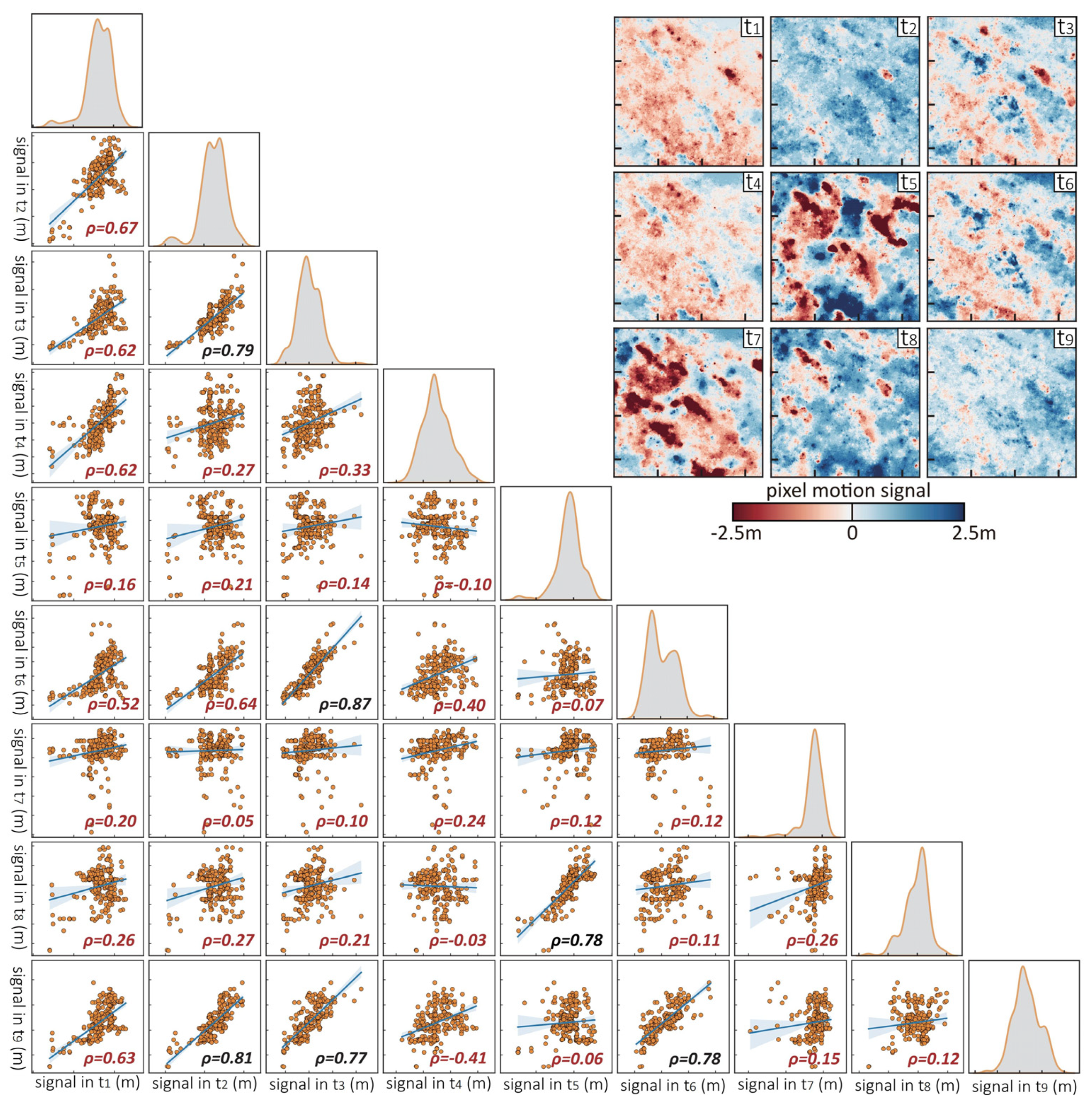
To effectively utilize a neural network to improve displacement detections, we must address two essential questions: “what to learn” and “how to learn”. Neural networks have demonstrated remarkable efficacy in InSAR deformation denoising tasks, attributed to their ability to differentiate between the distinct temporal characteristics of deformation and noise [34,36,38]. Similarly, in comparison to deriving surface displacement from a pair of optical images, the MPIC data may include temporal features from both the real displacement and the noise: in MPIC data, the former remains persistent and unchanging over time, whereas the latter exhibits weak and even no correlation in time [4,7,11,39]. As an illustration, Figure 1 shows the signals and their across-correlations within an actual MPIC derived from Sentinel-2 images. Given the absence of any significant earthquakes within the area during the image acquisition period, surface signals can be seen as correlated noises. These signals between the MPIC data exhibit strong randomness in time, as most of the correlation coefficients ($\rho$) are below 0.7 [Figure 1]. Consequently, we can design a neural network to separate displacement and noise by their temporal features in MPIC, thereby answering the question of “what to learn”. Subsequently, we need to solve the “how to learn” question.

2.2. Architecture of Neural Network

For the MPIC denoising task, we designed a neural network autoencoder that consists of four modules: input standardizing, encoding, decoding, and estimating accuracy.

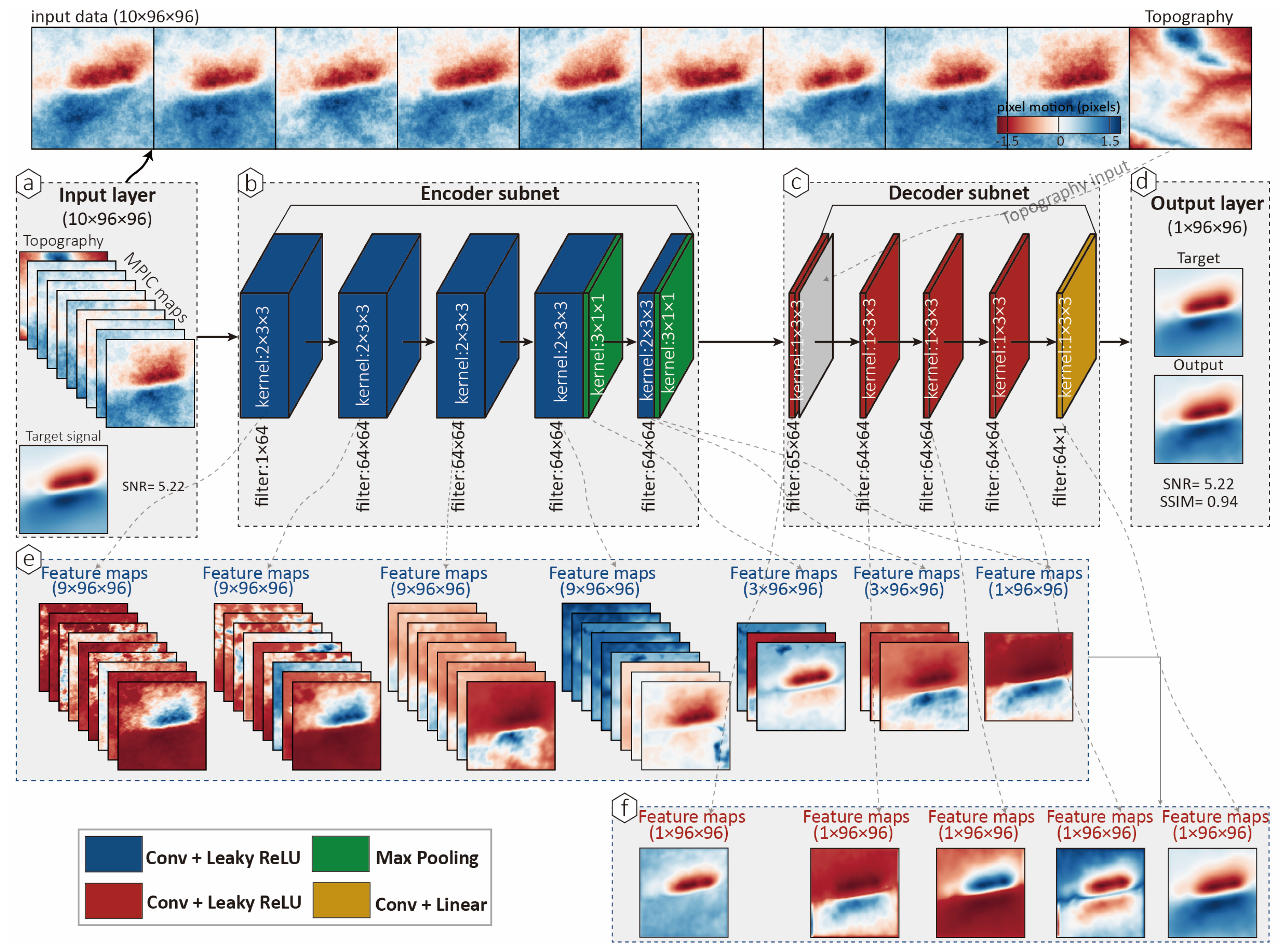
(1) Input layer: Instead of directly feeding raw data into the network, we first implemented a non-convolutional input layer to standardize input data prior to the training and testing stages. This can improve the network’s stability and generalization capacity because it reduces inconsistency of data distribution. The tensor size of the input data is [10 × H × W], where 10 identifies nine correlation maps (the input number of correlation map is determined by number of pooling operation and size of pooling kernel) and one topography data. Here, H and W denote the height and width of the input MPIC, respectively [Figure 2a]. The sizes of input correlation map and corresponding topography data thus are [9 × H × W] and [1 × H × W], respectively. Meanwhile, the layer labels target displacement and noise component of each input. It also calculates the signal-to-noise ratio (SNR) of each input, defined as the ratio of the root mean square of the displacement power to that of the noise power.

(2) Encoder subnet: Then, the standardized data is fed into the encoder. The encoder consists of five purely convolutional and two max-pooling layers [Figure 2b]. It encodes the input signals that are persistent in time, and yields feature representations with enriched information for the subsequent subnet. The convolutional kernel with size of 2 × 3 × 3 (one temporal dimension and two spatial dimensions) is employed to stack the input signals with different weights, which extracts localized feature representations of them. The input MPIC data comprise nine correlation maps along the temporal dimension. Two successive max-pooling layers with a kernel size of 3 × 1 × 1 are applied along the time axis to compress temporal information while keeping spatial dimensions unchanged. The first pooling operation reduces the temporal dimension from 9 to 3 by aggregating non-overlapping temporal windows of size three, and the second pooling further compresses it from 3 to 1. This hierarchical temporal pooling enables the network to integrate multi-temporal correlation information into a single representation [Figure 2b].

A limitation of the proposed framework lies in its restriction on the temporal dimension of the input MPIC data. Owing to the use of two temporal pooling operations with a fixed kernel size of 3 × 1 × 1, the current network architecture is designed to operate on inputs comprising exactly nine correlation maps and therefore does not directly support variable-length MPIC inputs. Each convolutional layer applies 64 different filters to the input and output to generate as many channels as feasible for feature extraction, except that the input of the first layer and the output of the last layer exclusively possess one filter [Figure 2b]. As such, each layer encompasses a significant number of trainable parameters given by n_kernel × n_input × n_output + n_output, where n_kernel is the kernel size (product of its shape in all dimensions), n_input and n_output are the number of input and output filters to the layer, respectively. The network’s nonlinearity is bolstered by incorporating a biased Leaky ReLU activation function in each layer.

(3) Decoder subnet: The decoder consisting of five purely convolutional layers is employed to reconstruct the denoised displacement using the feature representations generated by the encoder [Figure 2c]. As the temporal dimension has been eliminated through the max-pooling operations during encoding, the decoder utilizes the convolutional kernel of size 1 × 3 × 3 (two spatial dimensions), focusing solely on reconstructing the spatial representation of the input feature created by the encoder. Each layer has the same filters as the encoder, except for only one output filter in the last layer.

The topography data is added as a secondary input. Terrain information is incorporated into the network as an additional input channel of size 1 × H × W, which is concatenated with the MPIC channels at the input level. This channel-wise concatenation allows the terrain data to be processed jointly with the MPIC data in the decoder through standard convolutional operations, enabling the network to learn terrain-related noise features together with deformation patterns. No explicit fusion strategy (e.g., attention mechanisms or intermediate feature stitching) is employed in the decoder. Instead, the influence of terrain-related noises is implicitly integrated into the reconstructed displacement field through the shared feature representations, which can remove the topographically correlated noises or errors. The last layer employs a linear activation function, ensuring that positive and negative displacement signals are equally reproduced.

(4) Output layer: Lastly, the output layer is designed for a range of tasks, i.e., de-standardization of the output, estimation of denoising accuracy, and visualizations of the input and output [Figure 2d]. For denoising accuracy estimation, we calculated the structural similarity index (SSIM) between the target and output displacements. The SSIM is adopted as the loss function in this study. Unlike pixel-wise losses such as MSE or L1, which primarily penalize local amplitude differences and may lead to over-smoothing, SSIM emphasizes the preservation of spatial structures, local gradients, and contrast. For MPIC displacement fields, maintaining the spatial continuity and coherent deformation patterns is more critical than minimizing point-wise errors alone. Although SSIM was originally developed for image quality assessment, it has been widely used in image reconstruction and denoising tasks where structural fidelity is essential. Here, SSIM-based loss encourages the network to recover physically meaningful deformation structures rather than optimizing absolute displacement values only. The SSIM, ranging from 0 to 1, is a common denoising evaluation metric in image processing. A higher SSIM denotes that the output displacement matches the target better, hence better network performance [40,41].

2.3. Loss Function

During the training stage, a loss function is commonly employed to supervise the network training. In our study, we define the loss function as: loss = 1 − SSIM. The minimization of the loss function is solved with an iterative back propagation method using the Adam optimizer during model training [42]. Notably, the feature maps of one channel generated by our network suggest that it can effectively extract features of progressive complexity from the input to the output layers, and recognize signals that are persistent in time by progressively removing the time dimension of the input while considering temporally unstable signals as correlated noise [Figure 2e,f]. Thus, our devised neural network and loss function yield effectiveness in addressing MPIC denoising tasks, thereby addressing the question of “how to learn.”

3. Training and Testing Datasets

3.1. Simulation of MPIC Noise Datasets

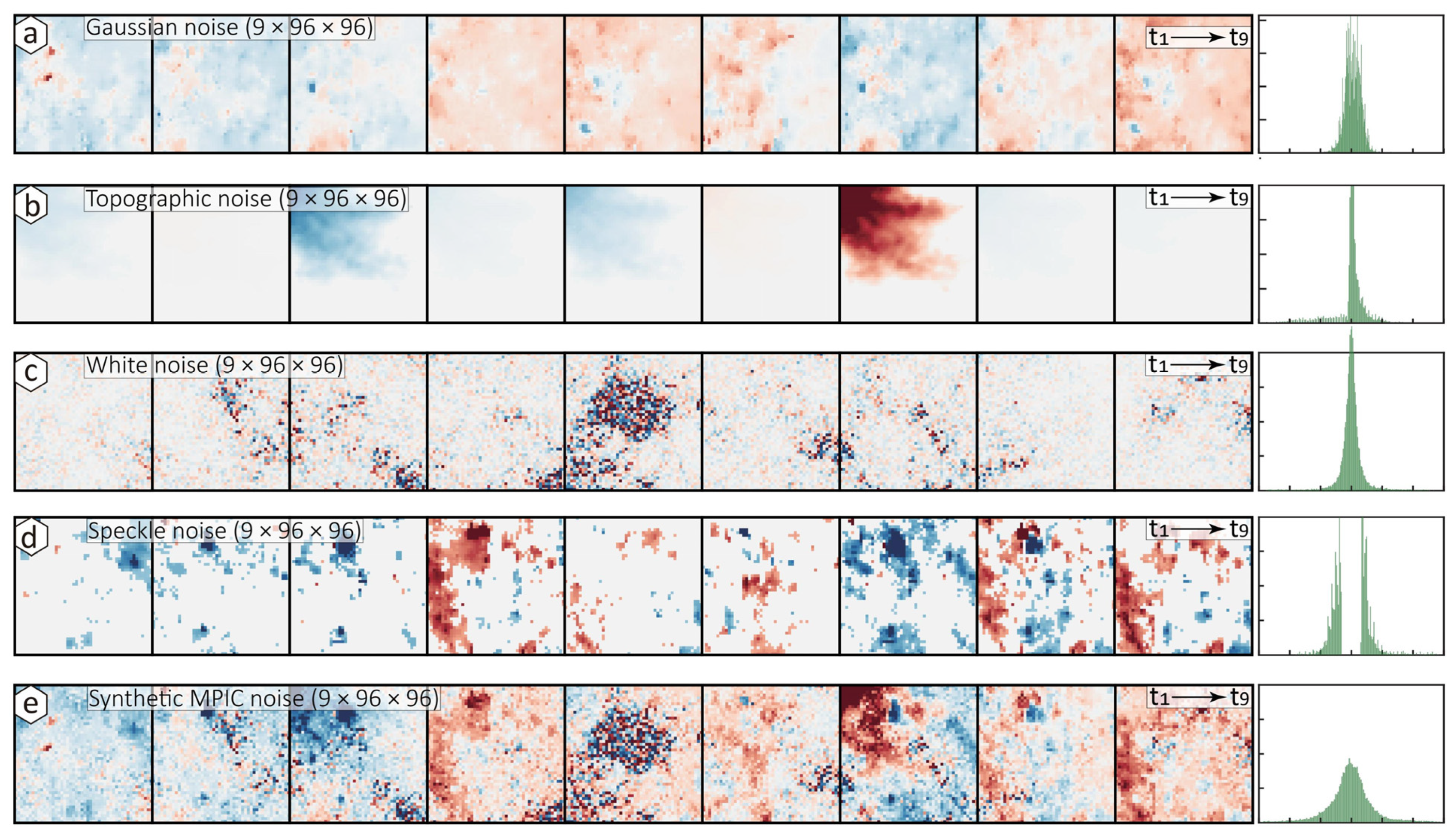
To achieve expected performance, neural networks often require training on comprehensive and reliable datasets. The most common approach of creating training datasets is to simulate synthetic data. For instance, the InSAR noises can be simulated by shearing similar properties observed in actual observations [36,38]. Similarly, correlated noises in MPIC can be realistically simulated, as their physical origins and statistical properties are well understood. To generate correlated noise fields covering the area shown in Figure 1, we synthesize several major MPIC noise components. Specifically, spatially correlated Gaussian noise is introduced to mimic residual artifacts arising from imperfect image co-registration, matching uncertainty, and other systematic processing errors [Figure 3a]. Topographically correlated signals are generated using digital elevation model (DEM) data covering the study area to represent topographic errors and geometry-related distortions in optical imaging [Figure 3b]. In addition, local additive white noise is incorporated to model random noise components associated with sensor noise and pixel-level uncertainties [Figure 3c]. Furthermore, low-pass mean noise combined with varying illumination directions is employed to create shaded-relief effects, thereby simulating speckling, blurring, and illumination intensity variations commonly observed in optical imagery [Figure 3d]. The final synthetic noise field is constructed as the linear summation of all above noise components, providing a realistic representation of the complex noise characteristics in MPIC data [Figure 3e].

One of the advantages of employing synthetic noise to train neural networks is that it can generate a large volume of data that is usually not available for the real data. Nonetheless, the resemblance between the synthetic and real data significantly impacts how well the neural network will perform on real data. The statistical features of the synthetic and real noises [Figure 1 and Figure 3e] suggest that they both are nearly Gaussian. However, these two noises are largely uncorrelated (R² = 0.12), meaning that the synthetic one may not accurately represent the real one. This difference might result in the autoencoder trained with synthetic data being unable to generalize effectively to real data. To further understand the potential discrepancy, we simulated a synthetic noise dataset to train and test our neural network (a total of 1.1 million, each size = [9 × 96 × 96]), allowing for a comparison of denoising performance trained on synthetic and real noise datasets [Figure 3e]. Moreover, we collected the 12.5 m digital elevation model from Advanced Land Observing Satellite to generate 1.1 million topography samples (each size = [1 × 96 × 96]). These topography samples were used to simulate topographically correlated signals and will be used as the topography input of each data to train and test our network.

3.2. Generating Training and Testing Datasets

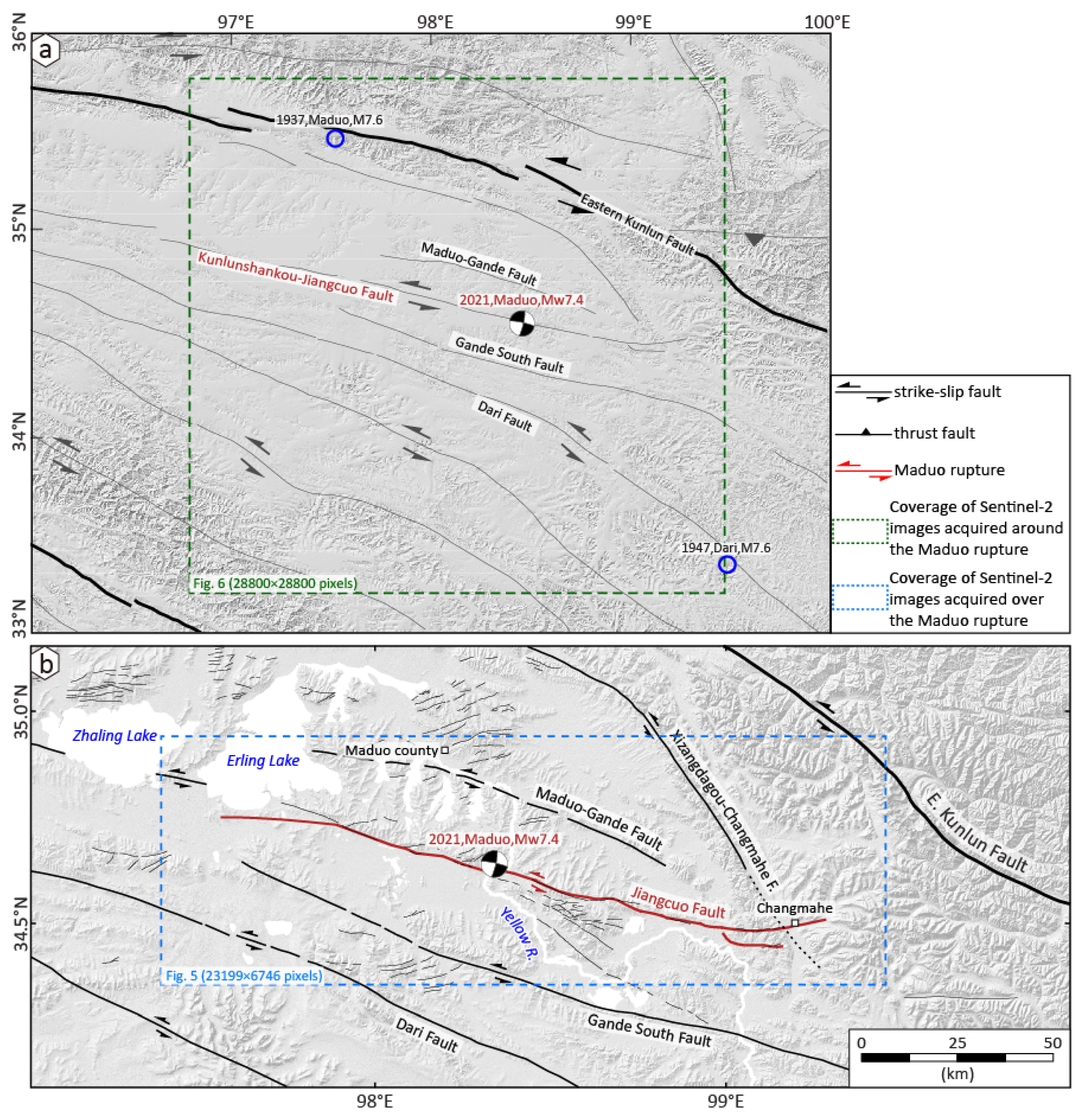
Another common method is to generate training and testing datasets from real observations. The rapidly growing and now publicly available Sentinel-2 imagery provides a large amount of images to create real MPIC datasets. Here, we generated training and testing MPIC datasets built from the Sentinel-2 images over and around the 2021 Maduo earthquake [Figure 4].

(1) Tectonic setting and study area: On 21 May 2021, the Mw7.4 Maduo earthquake occurred in the eastern segment of the Kunlunshankou-Jiangcuo Fault, a sinistral fault that connects with the fast-slipping Eastern Kunlun Fault in the Tibet Plateau [Figure 4a] [43,44,45,46,47,48]. Geodetic observations revealed a detailed surface rupture over a distance of 150 km along the Jiangcuo fault, with surface displacement mostly close to or even less than 1 m [Figure 4b] [46]. Applying subpixel correlation to the Sentinel-2 imagery with a ground pixel size of 10 m, the lower limit of the detectable displacement amplitude is ~1 m. This indicates that the correlated noise between Sentinel-2 acquisitions may present a big challenge to detect surface displacement close to 1 m accurately. Since the low-cloud-coverage images acquired before and after the earthquake repeatedly covered the Maduo area and its surroundings, this provides sufficient data to generate training and testing datasets. Additionally, this large amount of data (i.e., GPS and InSAR data) provides an opportunity to verify our model performance by comparing the results with these independent datasets.

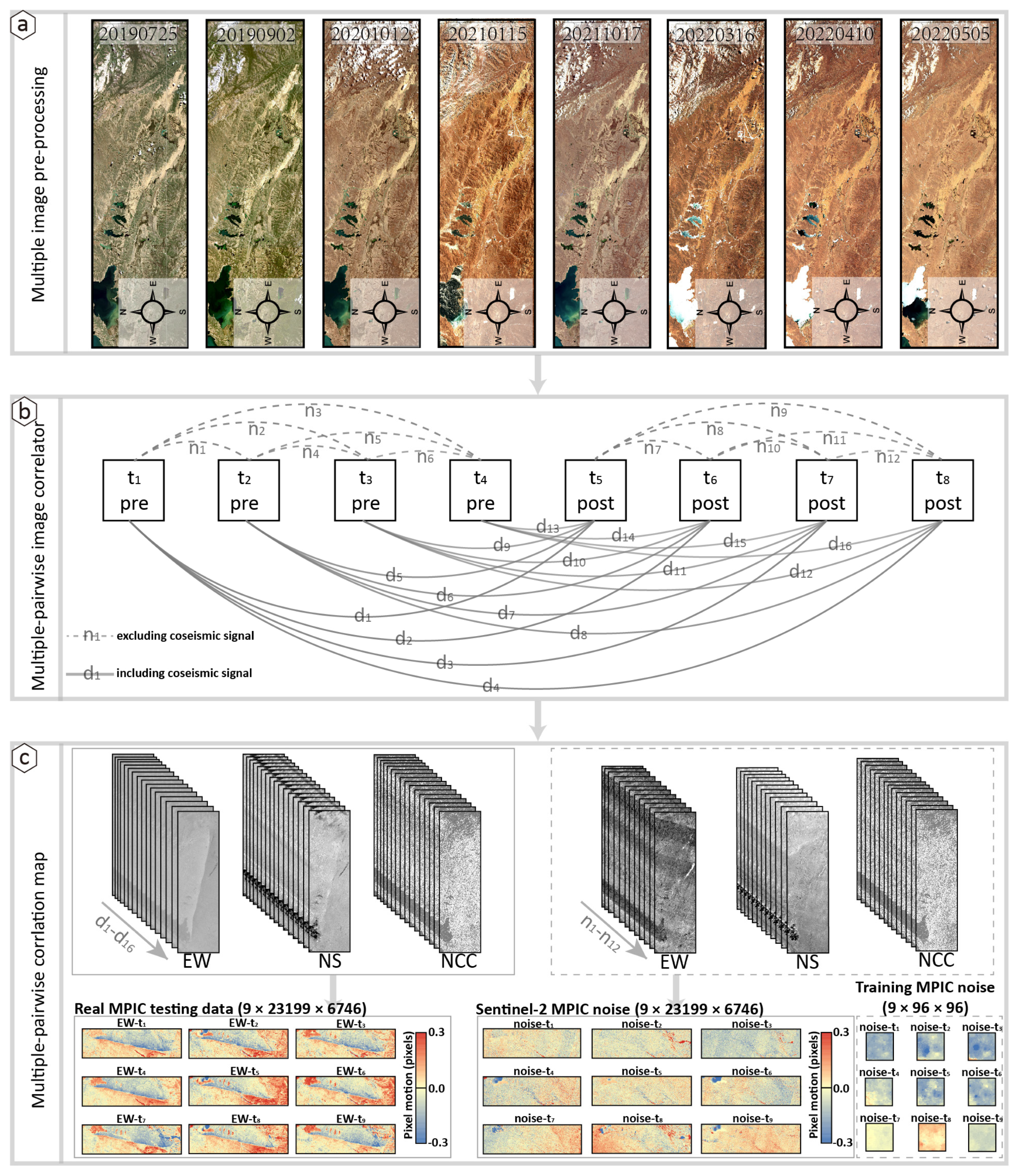
(2) MPIC datasets over the Maduo rupture: To generate training and testing datasets, we implemented optical MPIC processing in the MicMac open-source library. 6illustrates the MPIC processing chain. Consistent settings were used to capture surface signals, including a sliding window of 3 × 3 pixels, a step of one pixel, and a regularization term of 0.5, which results in EW and NS correlation maps with a 10 m pixel resolution [6,49]. The Sentinel-2 images were publicly available through the Google Earth Engine platform [50]. With eight images acquired before and after the earthquake over the Maduo rupture [Figure 4b and Figure 5a], we obtained 16 EW and NS displacement maps from pre- and post-event images, along with 12 EW and NS correlation maps from either pre- or post-event images [Figure 5b]. Then, we randomly selected nine displacement maps to construct the EW and NS MPICs, respectively [Figure 5c]. This serves as real testing cases to validate the network’s generalization performance.

(3) Generations of MPIC noise datasets: Because the network relies on different temporal signatures to remove noise and recover displacement, it categorizes everything in MPIC that is inconsistent with the temporal features of coseismic displacement as noise. The ground signals generated from the Sentinel-2 images that are acquired during a period without large earthquakes are considered as correlated noises. For instance, the 12 correlation maps above are treated as a good representation of the noise because signals of the Maduo earthquake were excluded [Figure 5c]. Every time we non-repetitively extracted nine correlation maps from 12 pre-/post-event pairs to create one MPIC noise data (size of [9 × 23,199 × 6746]). Through multiple random but non-repeating combinations of the sampling, we constructed six MPIC noise data from 12 correlation maps covering the Maduo rupture. Then, the real MPIC noise was generated by sequentially intercepting a smaller area (each size = [9 × 96 × 96]) from the six MPIC noise data. The interception was conducted 100,000 times to generate the MPIC noise dataset for network training and testing [Figure 5c].

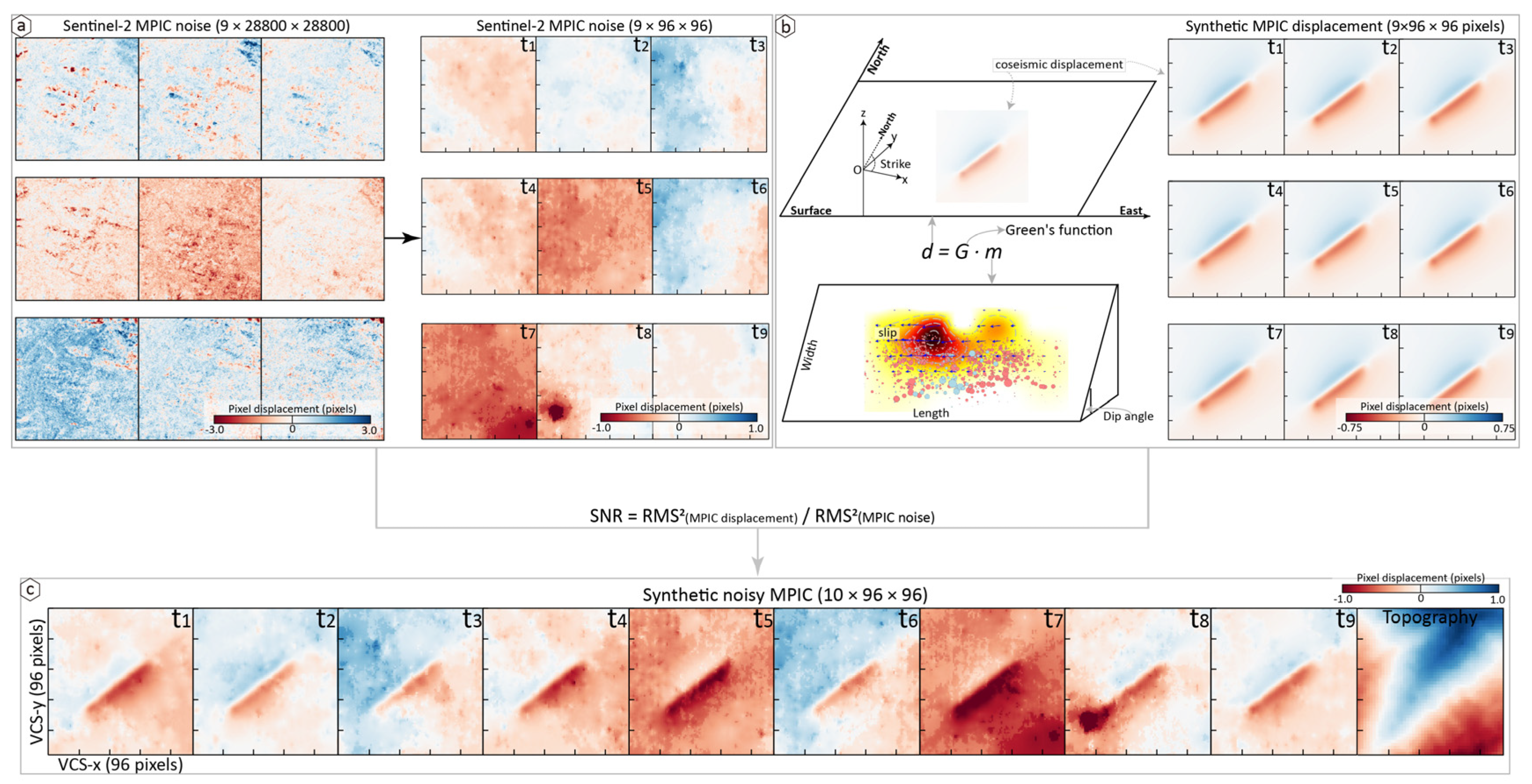
In addition, to provide a larger noise dataset for network training, we collected 21 Sentinel-2 images covering the Maduo area through the Google Earth Engine platform [Figure 4a]. Among these, 15 images were acquired before the Maduo earthquake, while six images were captured after the earthquake event. The image acquisitions also excluded other coseismic displacement signals that can be detected by the Sentinel-2 MPIC. We applied the same MPIC processing to capture 120 correlation maps from the pre-event or post-event image pairs. Every time we non-repetitively extracted nine correlation maps from 120 pre-/post-event correlation maps to create one MPIC noise data (each size of [9 × 28,800 × 28,800]). An example of the MPIC noise is presented in Figure 6a. Similar to the procedure in preparing the above noise dataset, an MPIC noise dataset containing one million samples (each size of [9 × 96 × 96]) was further intercepted from the 12 MPIC noise data, as illustrated in Figure 6a.

Overall, we generated a total of 1.1 million MPIC noise data, (each size of [9 × 96 × 96]) from the Sentinel-2 MPICs. Notably, during both training and testing stages, the noise will be added onto the displacement signal to mimic real perturbations that are desired to be removed.

3.3. Synthetic MPIC Displacement Data

The feature representations of coseismic displacement patterns need to be incorporated into the network. However, because of the unavailability of ground truth surface displacement data for optical MPIC, we used model predictions instead. We assumed that surface displacement was induced by fault slips that were buried in an Okada’s elastic half-space [51], with hypocentral positions at a random longitude and latitude within a virtual coordinate system (96 × 96 pixels) and a depth range of 3–20 km [Figure 6b]. The fault geometries and slips were uniformly distributed with following random variables: strike angle [0°, 360°], dip angle [60°, 90°], and rake angle for left-lateral [0°, ±45°] and for right-lateral [±135°, ±180°] scenarios. The moment magnitude is uniformly sampled within the range of [5.5, 8.5], and the corresponding fault length, width, and slip were generated using an empirical relationship derived from geodetic data [52]. As coseismic displacement does not change with time and persists in each correlation map of MPIC data, a single displacement can be extended into MPIC displacement (a total of 200,000) [Figure 6b]. Finally, we created a dataset consisting of 1.1 million noisy MPICs by adding the noise into the synthetic displacements [Figure 6c]. The dataset, together with corresponding topography data, will be fed into the input layer of the network for training and testing.

4. Training and Testing Neural Network

4.1. Training the Neural Network

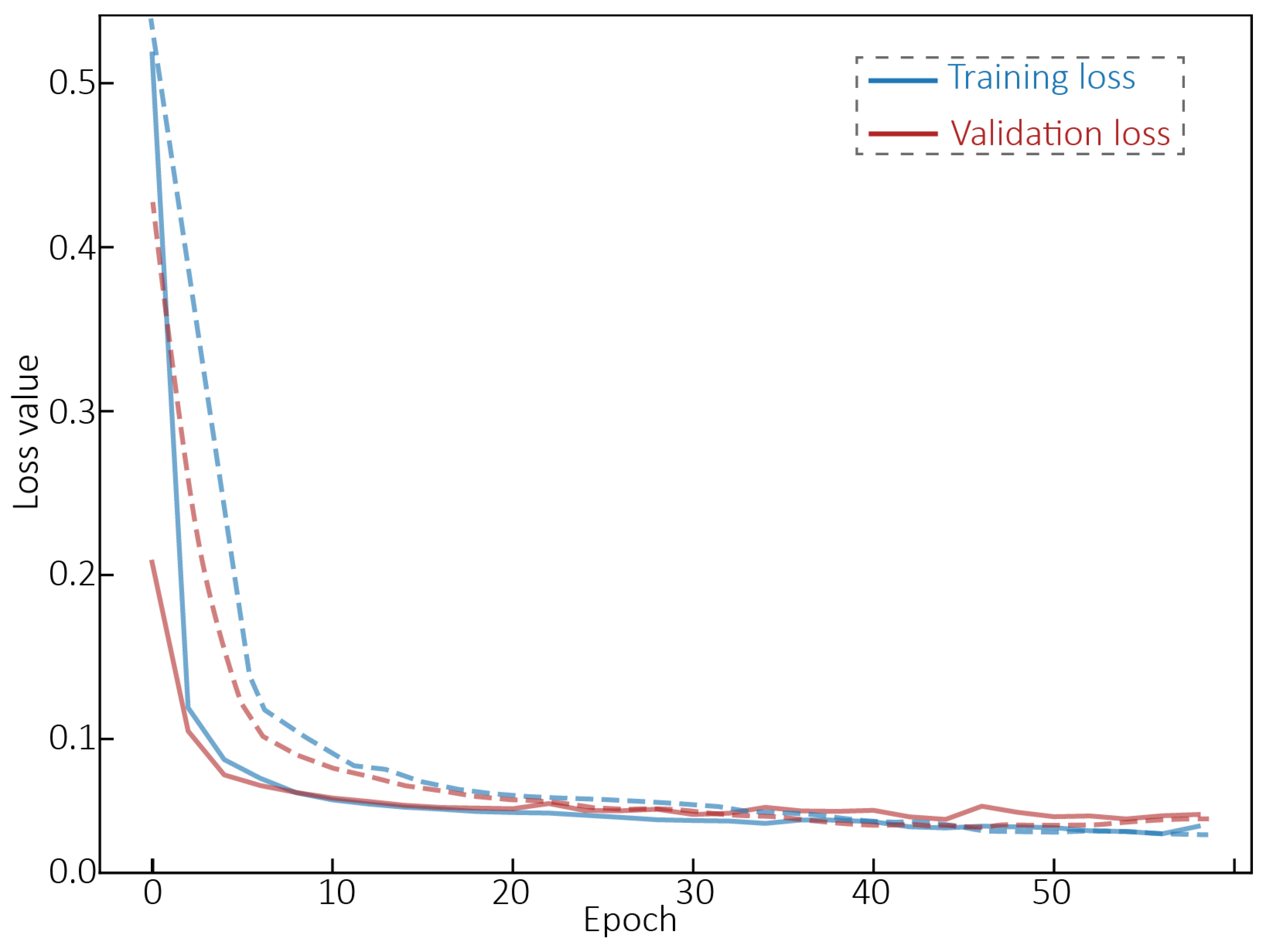
The training and subsequent testing tasks were conducted on a high-performance server with GPU accelerators using the Keras and Tensorflow Python libraries [53]. We randomly selected one million noisy MPICs from the 1.1 million sample dataset as the training dataset. The remaining 0.1 million samples constituted the testing dataset. During the network training stage, the training dataset was injected into our neural network, and then it was randomly split into two categories in the input layer: training (80% of the total number) and validating (the remaining 20%) subsets. Figure 7 shows the loss curve of the network during the training stage. As the training progresses, the loss gradually decreases and reaches a plateau on both the training and validation subsets, indicating the effective network training and optimization of parameters.

To further address another question about whether there are differences in denoising performance among the denoisers trained on real and synthetic MPIC noises, we also trained the neural network on the data with simulated noise using the same training strategies and operations applied to the actual noise. Similarly, the minimization of the loss function demonstrates the effectiveness of the network training [Figure 7]. After this training, the autoencoder trained on real noise data was referred as the (real) denoiser, and the one trained on synthetic noise data was referred as the synthetic denoiser.

4.2. Performance on MPIC with Simulated Noise

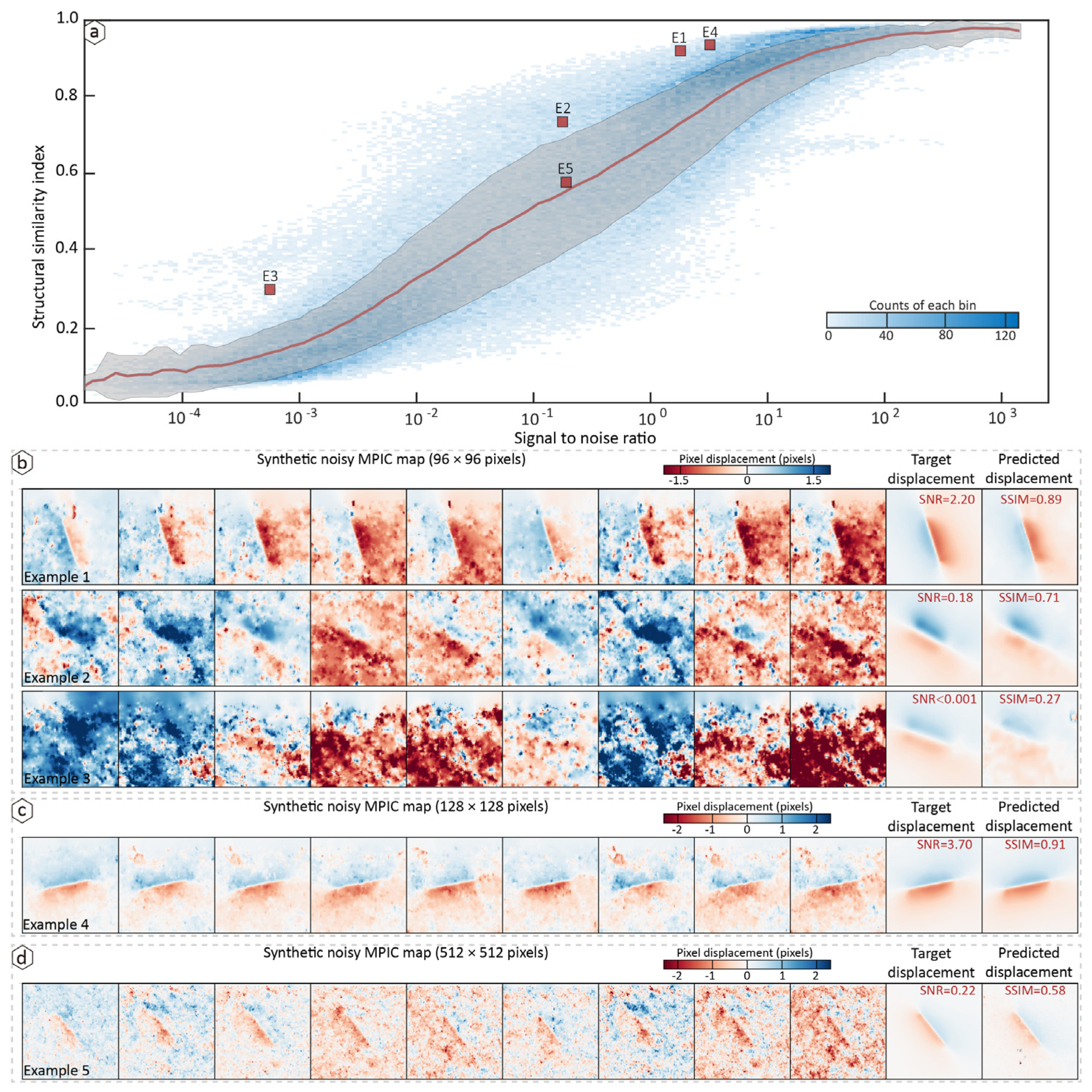
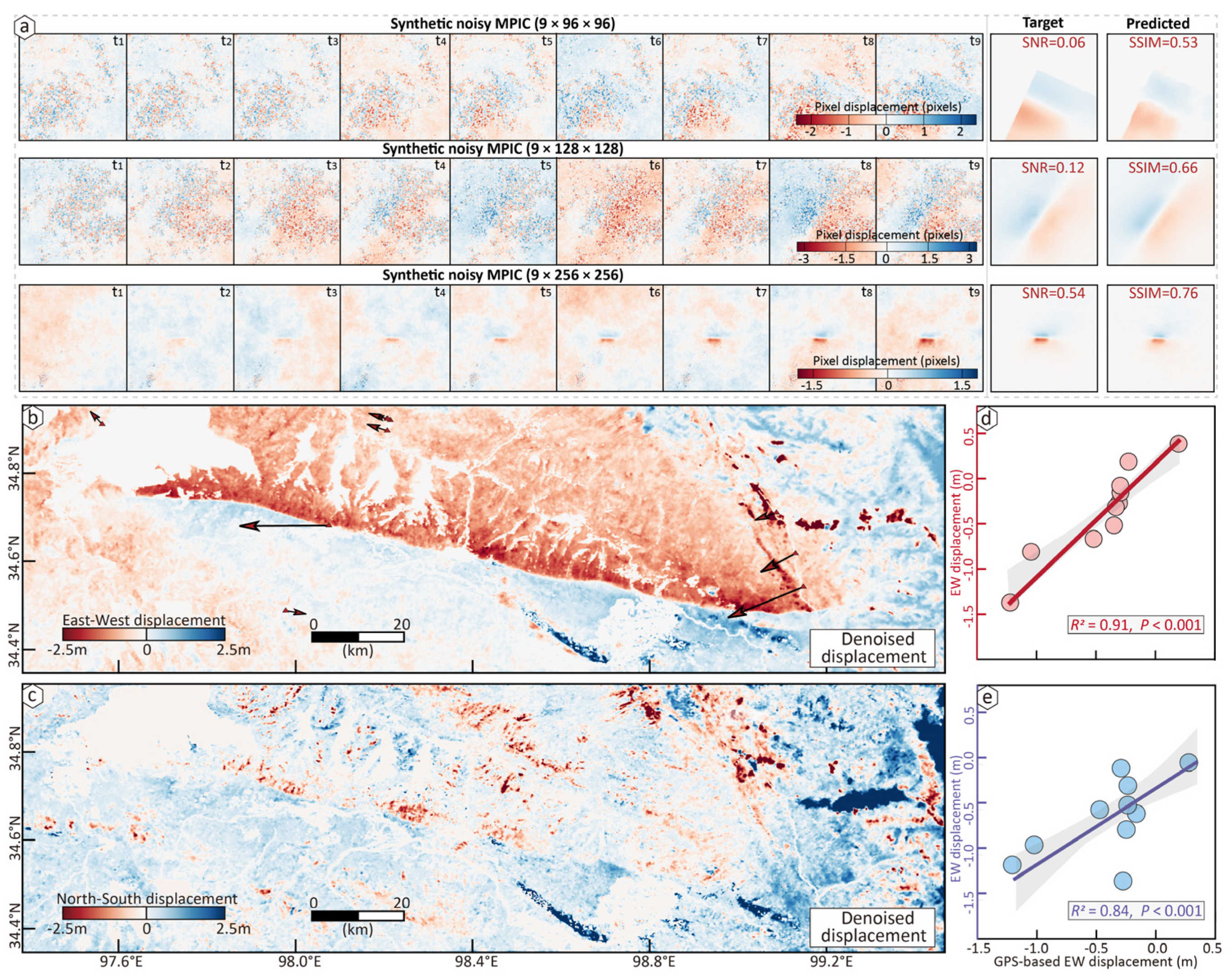
After network training, to test the denoising efficiency, we first applied it to our testing dataset that was not used during the training. To test whether the denoiser’s performance depends on the input size, the testing data also includes various spatial sizes, e.g., 48 × 48, 96 × 96, 128 × 128, and 256 × 256. The SSIM between target displacement and denoiser’s output was used to assess the denoising efficiency. Figure 8a illustrates the correlation between the SNR and the SSIM. As expected, the denoiser effectively eliminates the noises overlapping on the target displacement, providing denoised and accurate displacement patterns for the input (examples 1 and 4) [Figure 8b,c]. Even for data with low SNRs, where the target signal could not be visually discerned in the input MPICs, it still provided markedly improved reconstructions (SSIM > 0.5 in examples 2 and 5) [Figure 8b,d]. However, in some cases, the denoiser did not produce meaningful reconstructions due to extreme noise corruption (example 3 with the SNR below 0.01) [Figure 8b]. Notably, although the denoiser was trained using input patches of a fixed size (96 × 96 pixels), it can be applied to MPICs with different spatial dimensions in practice, owing to its fully convolutional architecture. This shows its fundamental ability to handle arbitrarily sized inputs. Generally, the denoiser can reconstruct the denoised displacements and accurately isolate the noises overlapping on displacement, without requiring human interventions or prior knowledge of the rupture kinematics.

4.3. Application to a Real Displacement: The 2019 Ridgecrest Earthquakes

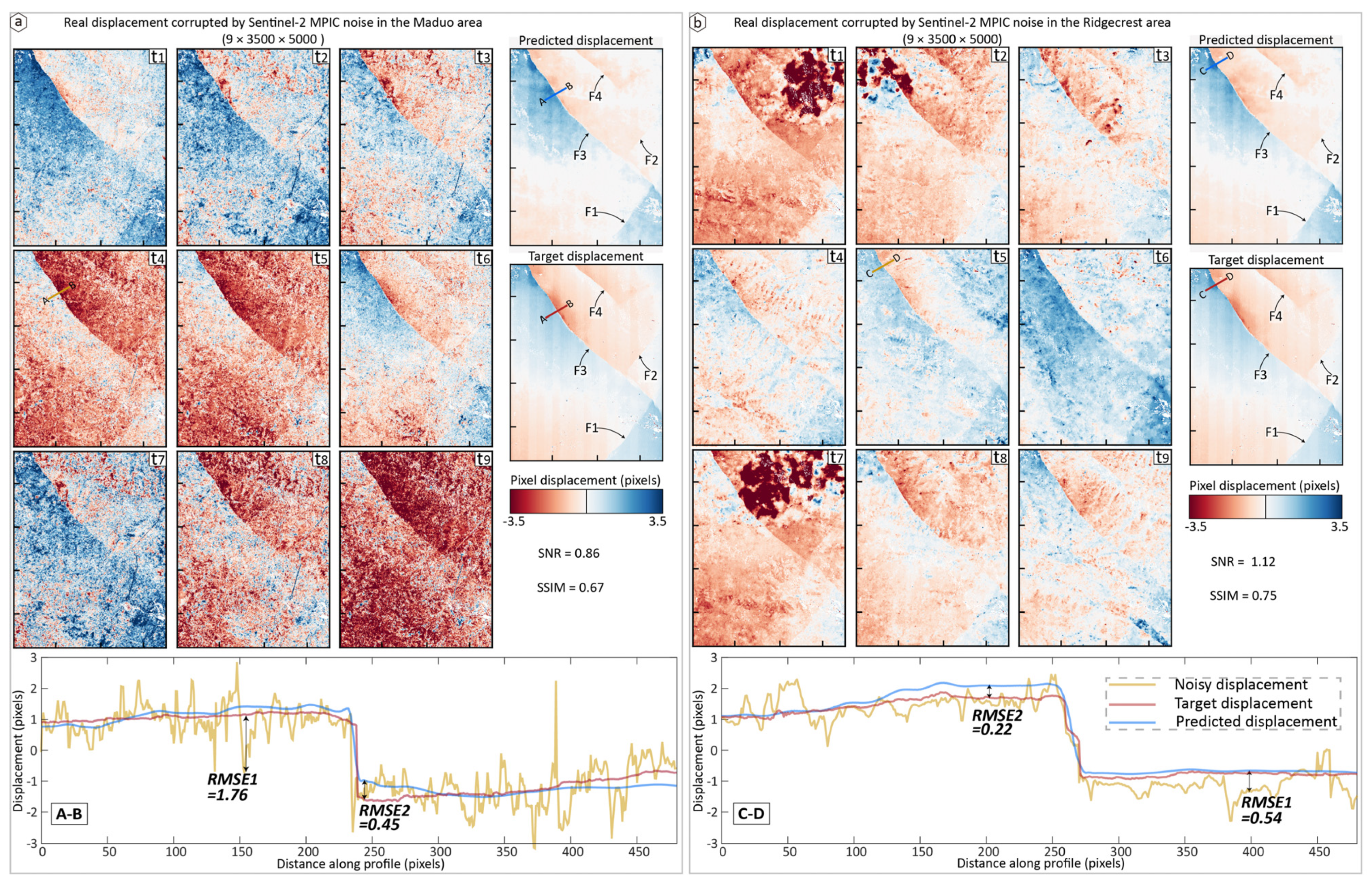
Moreover, we tested the denoiser on the real data that covers the multiple faults ruptured during the 2019 Ridgecrest earthquakes [3,11]. The optical displacement reported by Barnhart et al., 2020 [11] was seen as the target. The target displacement was corrupted with two MPIC noises: one from the Maduo area [Figure 9a], and the other generated using Sentinel-2 images acquired before the 2019 Ridgecrest event [Figure 9b]. The denoised displacements exhibited successful recovery of displacement signals in the input MPICs, with SNRs of 0.86 and 1.12, which were in good agreement with the targets (SSIMs of 0.67 and 0.75. Compared to the input MPICs, the denoised displacements revealed ruptures on multiple faults, F1–F4. Here we highlight the clear signals on the secondary faults F1, F2, and F4. As a result, the denoiser is capable of recovering intricate displacement patterns associated with multiple fault ruptures, which is a common scenario in large strike–slip earthquakes.

With the denoised data, the fault offsets can be accurately measured, as observed along the profiles AB and CD. The root mean squared errors of the input MPICs and the target were 1.76 and 0.54 pixels, respectively, which were significantly reduced to 0.45 and 0.22 pixels after denoising. Notably, the denoiser was trained with noise data from the Maduo area, yet it performed effectively on the MPIC corrupted by noises from the Ridgecrest area. The denoising performance on the data with noise from the Ridgecrest area is better than that from the Maduo area. Two primary factors contribute to this outcome. Firstly, the data with noise from the Ridgecrest area exhibits a higher SNR compared to that with the Maduo area. Secondly, the correlated noises resulting from sensor, orbital, ortho-rectification, topographic, and other errors are mostly independent of region. In another word, these noises are similar for different regions. The denoiser thus exhibits exceptional generalization performance, demonstrating its ability to apply to global Sentinel-2 MPIC maps without the need for additional training.

4.4. Application to a Real Testing Case: The 2021 Maduo Earthquake

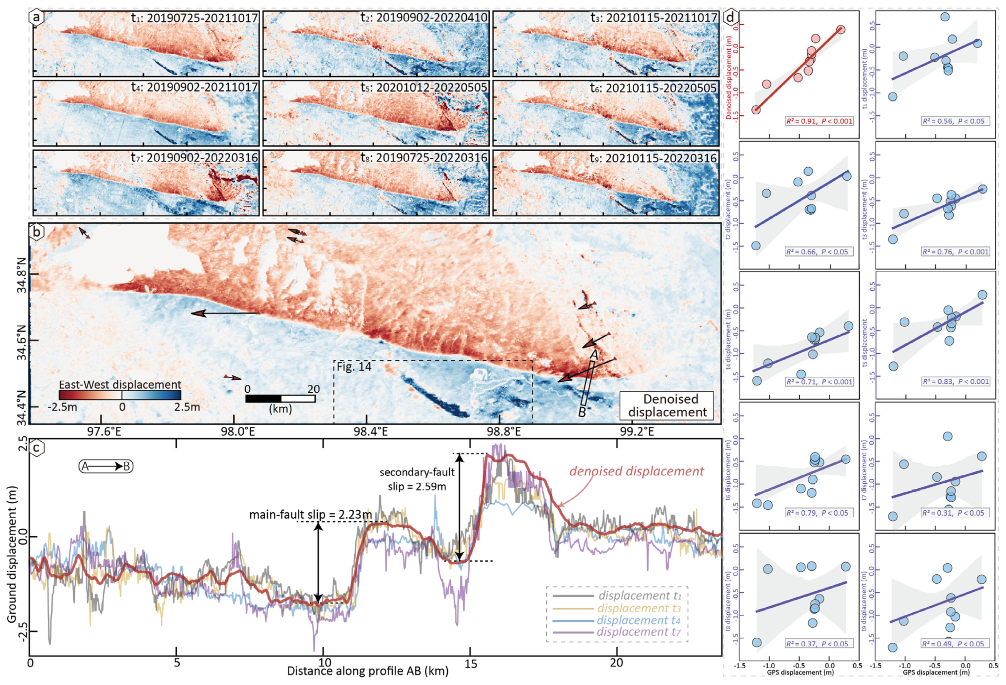
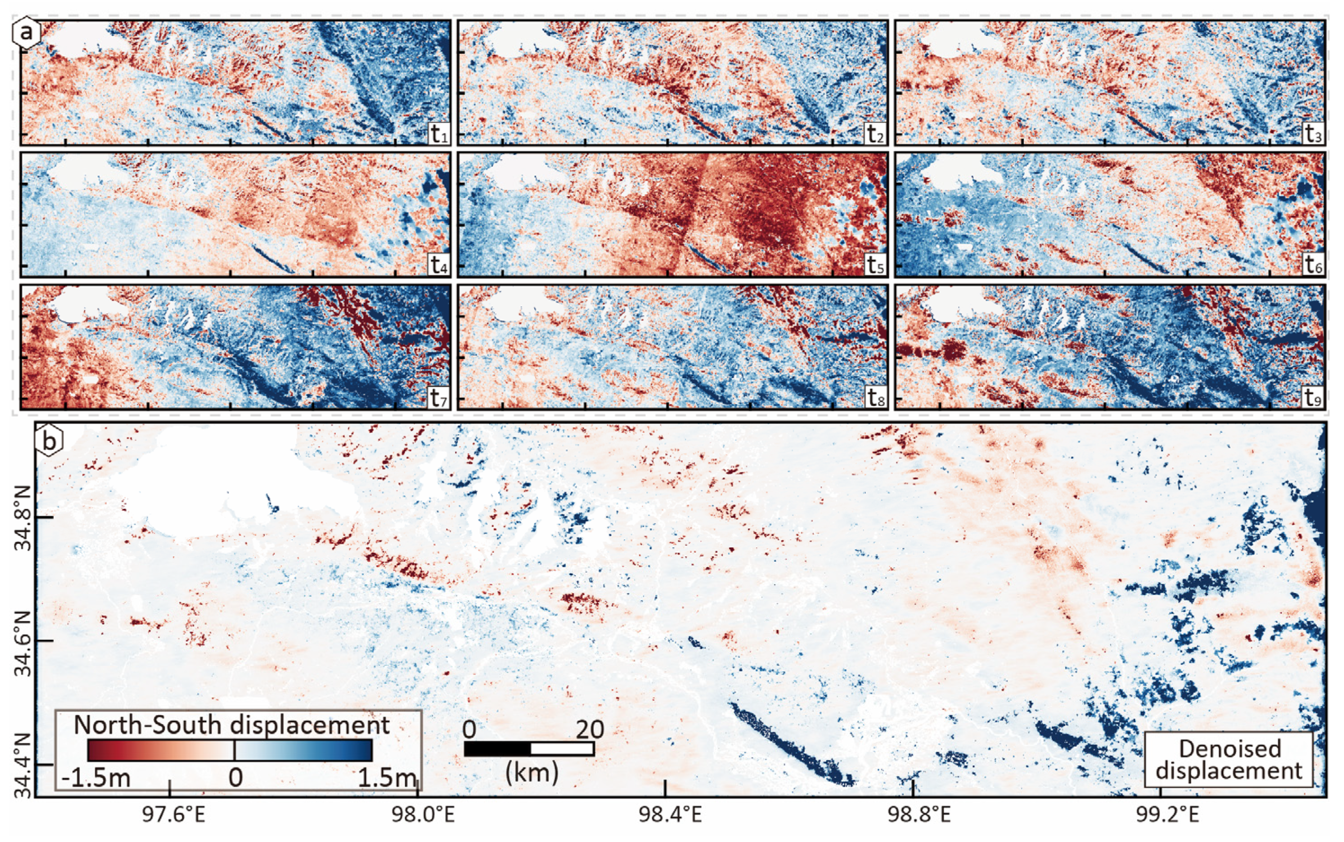
Finally, we assessed the denoiser’s general performance by applying it to real MPICs from the Maduo earthquake. The denoiser successfully recovered the clean EW and NS displacements from the raw MPICs [Figure 10 and Figure 11]. The denoised displacements exhibited significant improvements compared to the input, resulting from the efficient suppression of correlated noises. This improvement was notably pronounced in the NS displacement field, and at the eastern and western ends of the EW displacement. Figure 10c shows the input (t₁, t₃, t_4, and t₇) and denoised displacements along the across-fault profile AB. The denoised displacement more accurately revealed the offsets on the main and secondary faults (2.2 m and 2.6 m, respectively) than the original data. We also compared the denoised displacements with GPS-based displacements at 10 stations in the area [54], which reveals a higher correlation between the denoiser’s output and GPS-based displacements (R² = 0.91) than the input data (R² = 0.31–0.83 for t₁–t₉) [Figure 10d].

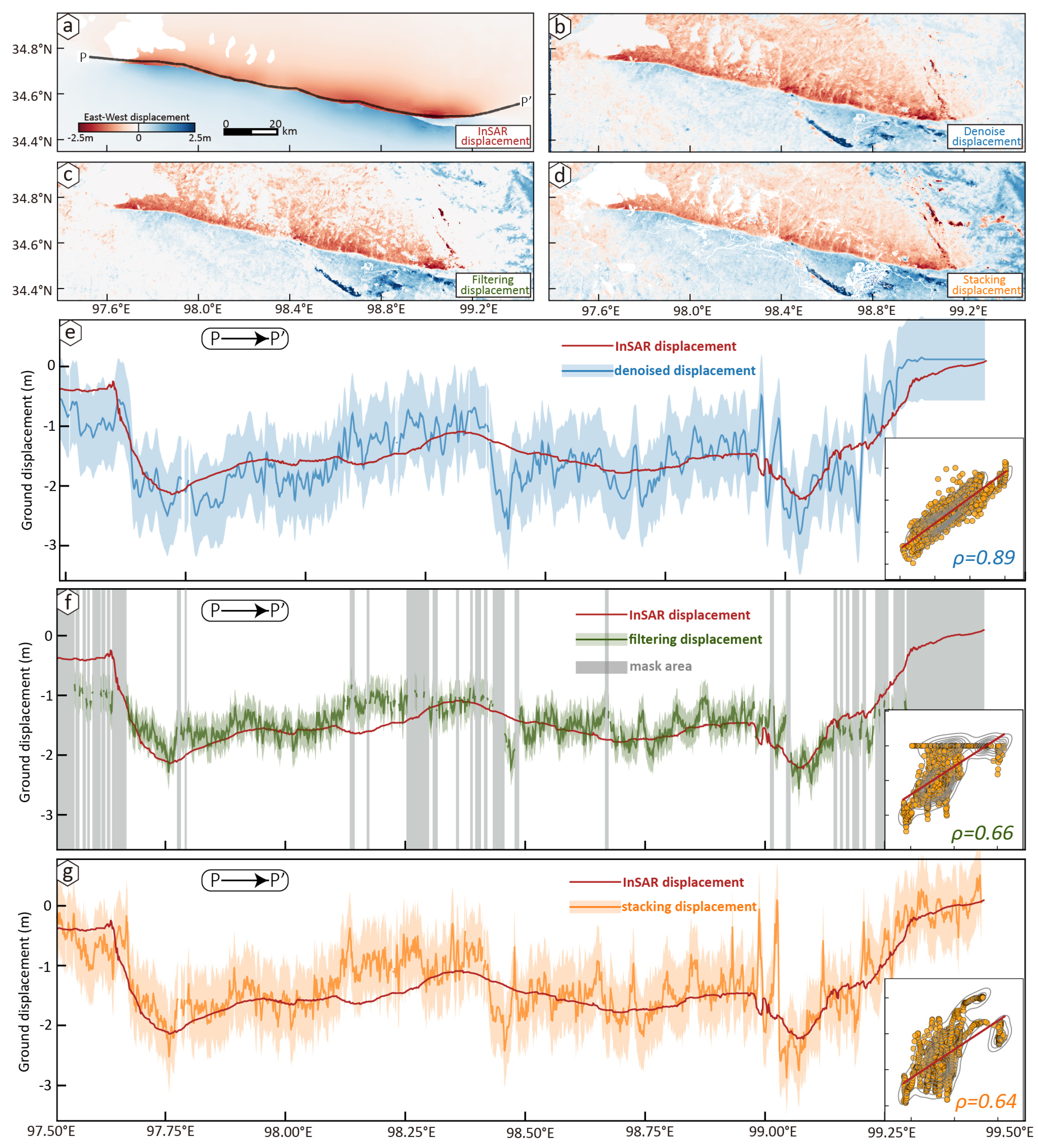
Furthermore, we compared the EW displacements resolved from InSAR-based deformations [45] with those reconstructed using our denoiser and that from two widely-used denoising techniques (i.e., temporal filter and stacking methods) [Figure 12a–d]. The correlation between the InSAR and denoised displacements (R² = 0.89) is 0.23 and 0.25 higher than the correlation between the InSAR and the displacements after the temporal filtering and stacking [Figure 12e,f]. The temporal filtering method removed some coseismic displacement signals at the gray stripe areas due to excessive filtering window length [Figure 12f]; conversely, the stacking displacement still exhibited considerable noise, particularly at the eastern end of the surface rupture [Figure 12g]. Consequently, the denoiser outperformed the traditional MPIC denoising methods, and has excellent generalization performance to reconstruct clean displacement patterns in real MPIC data.

5. Discussions

In general, neural networks trained on synthetic data with simulated noise can be generalized to real-world scenarios [34,35,36]. The broader the range of scenarios encompassed within the training data, the better the generalization performance when applied to real-world data. Despite that synthetic data has an advantage in overcoming the small volume of observed data, there is always a domain gap (that is, the significant differences in the data distribution and component used for training and testing data) between synthetic and real-world data [35]. This domain gap arises from inherent differences in data distributions, noise characteristics, and underlying processes between the synthetic and real environments. As a result, some signal patterns are observed but have not yet been simulated. For example, the non-atmospheric InSAR noises are only reproduced into neural networks by the real interferograms, because they cannot be accurately simulated using plausible approximations of real scenarios [35]. When training the network on just the simulated noise, it may not generalize well when applied to real scenarios due to including unseen samples.

To validate the performances of the denoiser trained on the simulated noise, we applied it to synthetic and real MPICs. The results indicate that it can provide accurate reconstructions of the input MPICs, performing almost as well as the real denoiser (SNRs < 1.0) [Figure 13a]. However, for the real MPICs, despite recovering the primary pattern of the Maduo earthquake displacements [Figure 10a and Figure 11a], the synthetic denoiser fails to remove the correlated noises completely, such as remaining noise signals in the eastern and western ends of the Maduo rupture and NS displacement [Figure 13b,c]. In contrast, the real denoiser performs more thorough noise removal in these areas [Figure 10b and Figure 11b]. Additionally, the real denoiser’s reconstruction exhibits stronger consistency with GPS-based displacements compared to the synthetic denoiser [Figure 13d,e]. Consequently, the real denoiser demonstrates superior generalization capabilities on real data in comparison to the synthetic denoiser. This inherent trait is crucial for effectively applying the denoising approach to any actual MPIC scenarios.

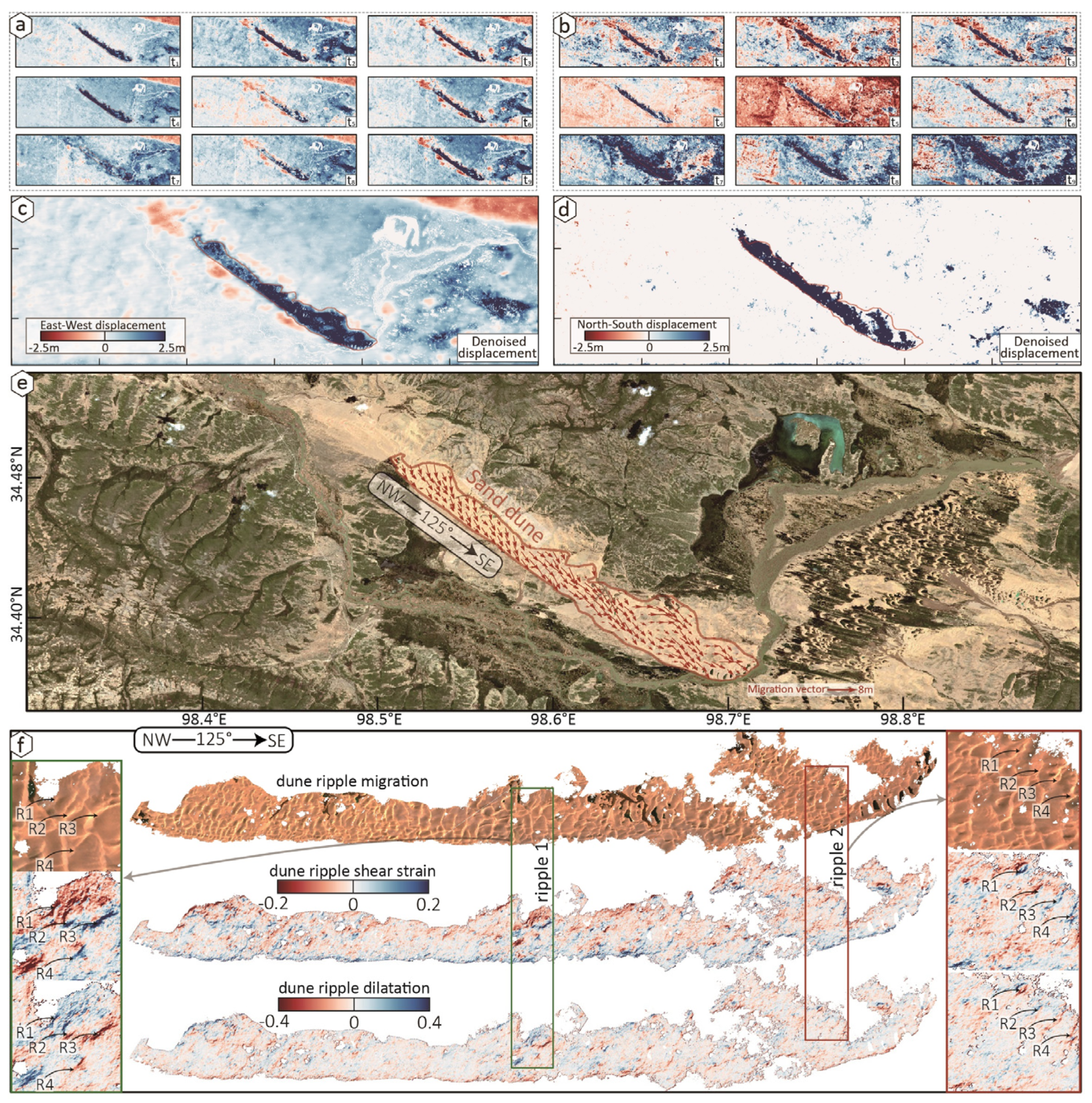
Additionally, we observed a remaining signal at the south of the Maduo rupture in all the denoised, temporal filtering, and stacking displacements [Figure 10, Figure 11 and Figure 12]. However, the geological and geodetic observations evidenced that this signal cannot be attributed to the Maduo earthquake [43,44,45,46,47]. The signal exhibits persistence in input EW and NS MPICs, and hence its temporal feature aligns well with the displacement feature learned by the denoiser [Figure 14a,b]. As a result, the denoiser not only preserved this signal but also provided a denoised displacement pattern for it [Figure 14c,d]. Interestingly, the first-order displacement pattern of the signal is highly correlated to the bedforms and ripples of a dune [Figure 14e]. This demonstrates that the signal was caused by the migrating dune near the Maduo rupture. The 27 km in length dune was identified to have a maximum migration of ~15 m over the period covered by the Sentinel-2 image acquisitions, with an overall migration azimuth of NW125°SE. Our denoiser indeed improved displacement signals for the dune ripples, where such complete and denoised measurement was previously not available.

Previous applications demonstrated that the optical image correlation measurement is quite efficient to detect dune motions [6,55,56,57]. Thus, the high-quality and denoised dune migration signals will also be greatly valuable for this detection. For instance, inverting the denoised displacements into the shear strain and dilatation fields [11], the migrating ripples and transport pathways can be visually identified and directly tracked without time-consuming manual intervention, such as at the ripple 1 and 2 areas [Figure 14f]. This is of major interest, as the denoised dune migrations provided would markedly reduce the detection bias of migrations, which can improve our interpretations of how various dune forms and their morphometric characteristics emerge [58,59]. In general, this clean dune migration signal demonstrates the application potential of our deep learning denoiser in improving the measurement accuracy of other tectonic processes such as slow landslides, glacier flows, and dune migration.

6. Conclusions

In this study, we trained and tested a deep learning denoiser to autonomously improve surface displacement in input MPIC, which is applicable if at least nine optical image correlation maps are available. The denoiser was effectively trained with a noise dataset created from Sentinel-2 images that exclude earthquake displacement signals. When applied to both the synthetic and real MPICs (e.g., the Ridgecrest and Maduo events), the denoiser can effectively remove correlated noises in the input MPICs, and accurately reconstruct denoised surface displacement, without any manual intervention or a priori knowledge of fault kinematics. The denoiser’s performance is significantly superior to the temporal filtering and stacking methods. Importantly, the denoiser trained on real noises allows for more stable and effective operation when applied to real MPICs than that trained on synthetic noises. Furthermore, the denoiser can also recover the clean surface signal associated with a dune near the Maduo rupture, revealing a previously unreported migrating feature. Therefore, the neural network holds great promise to reconstruct denoised horizontal displacements induced by tectonic or geomorphological processes like earthquake ruptures, glacier flows, dune migrations, and slow landslides.

References

1. Elliott, J.R.; Walters, R.J.; Wright, T.J. The role of space-based observation in understanding and responding to active tectonics and earthquakes. Nat. Commun. 2016, 7, 13844. [Google Scholar] [CrossRef] [Scilit]
2. Marchandon, M.; Vergnolle, M.; Sudhaus, H.; Cavalié, O. Fault geometry and slip distribution at depth of the 1997 Mw7.2 Zirkuh earthquake: Contribution of near-field displacement data. J. Geophys. Res. Solid Earth 2018, 123, 1904–1924. [Google Scholar] [CrossRef] [Scilit]
3. Milliner, C.; Donnellan, A.; Aati, S.; Avouac, J.-A.; Zinke, R.; Dolan, J.F.; Wang, K.; Bürgmann, R. Bookshelf kinematics and the effect of dilatation on fault zone inelastic deformation: Examples from optical image correlation measurements of the 2019 Ridgecrest earthquake sequence. J. Geophys. Res. Solid Earth 2021, 126, e2020JB020551. [Google Scholar] [CrossRef] [Scilit]
4. Socquet, A.; Hollingsworth, J.; Pathier, E.; Bouchon, M. Evidence of supershear during the 2018 magnitude 7.5 Palu earthquake from space geodesy. Nat. Geosci. 2019, 12, 192–199. [Google Scholar] [CrossRef] [Scilit]
5. Klinger, Y.; Okubo, K.; Vallage, A.; Champenois, J.; Delorme, A.; Rougier, E.; Lei, Z.; Knight, E.E.; Munjiza, A.; Satriano, C.; et al. Earthquake damage patterns resolve complex rupture processes. Geophys. Res. Lett. 2018, 45, 10–279. [Google Scholar] [CrossRef] [Scilit]
6. Rosu, A.-M.; Pierrot-Deseilligny, M.; Delorme, A.; Binet, R.; Klinger, Y. Measurement of surface displacement from optical satellite image correlation using the free open-source software MicMac. ISPRS J. Photogramm. Remote Sens. 2015, 100, 48–59. [Google Scholar] [CrossRef] [Scilit]
7. Provost, F.; Michéa, D.; Malet, J.-P.; Boissier, E.; Pointal, E.; Stumpf, A.; Pacini, F.; Doin, M.-P.; Lacroix, P.; Proy, C.; et al. Terrain deformation measurements from optical satellite imagery: The MPIC-OPT processing services for geohazards monitoring. Remote Sens. Environ. 2022, 274, 112949. [Google Scholar] [CrossRef] [Scilit]
8. Avouac, J.P.; Ayoub, F.; Leprince, S.; Konca, O.; Helmberger, D. The 2005, Mw7.6 Kashmir earthquake: Sub-pixel correlation of ASTER images and seismic waveforms analysis. Earth Planet. Sci. Lett. 2006, 249, 514–528. [Google Scholar] [CrossRef] [Scilit]
9. Antoine, S.L.; Klinger, Y.; Delorme, A.; Gold, R.F. Off-Fault Deformation in Regions of Complex Fault Geometries: The 2013, Mw7.7, Baluchistan Rupture (Pakistan). J. Geophys. Res. Solid Earth 2022, 127, e2022JB024480. [Google Scholar] [CrossRef] [Scilit]
10. Lauer, B.; Grandin, R.; Klinger, Y. Fault geometry and slip distribution of the 2013 Mw7.7 Balochistan earthquake from inversions of SAR and optical data. J. Geophys. Res. Solid Earth 2020, 125, e2019JB018380. [Google Scholar] [CrossRef] [Scilit]
11. Barnhart, W.D.; Gold, R.D.; Hollingsworth, J. Localized fault-zone dilatancy and surface inelasticity of the 2019 Ridgecrest earthquakes. Nat. Geosci. 2020, 13, 699–704. [Google Scholar] [CrossRef] [Scilit]
12. Liu, J.G.; Mason, P.J.; Ma, J. Measurement of the left-lateral displacement of Ms 8.1 Kunlun earthquake on 14 November 2001 using Landsat-7 ETM+ imagery. Int. J. Remote Sens. 2006, 27, 1875–1891. [Google Scholar] [CrossRef] [Scilit]
13. Avouac, J.P.; Leprince, S. Geodetic Imaging Using Optical Systems. In Geodesy; Elsevier Inc.: Amsterdam, The Netherlands, 2015; pp. 387–424. [Google Scholar]
14. Beyer, R.A.; Alexandrov, O.; McMichael, S. The Ames Stereo Pipeline: NASA’s open source software for deriving and processing terrain data. Earth Space Sci. 2018, 5, 537–548. [Google Scholar] [CrossRef] [Scilit]
15. Stumpf, A.; Michéa, D.; Malet, J.-P. Improved co-registration of Sentinel-2 and Landsat-8 imagery for Earth surface motion measurements. Remote Sens. 2018, 10, 160. [Google Scholar] [CrossRef] [Scilit]
16. Leprince, S.; Musé, P.; Avouac, J.-P. In-flight CCD distortion calibration for pushbroom satellites based on subpixel correlation. IEEE Trans. Geosci. Remote Sens. 2008, 46, 2675–2683. [Google Scholar] [CrossRef]
17. Ding, C.; Feng, G.; Li, Z.; Shan, X.; Du, Y.; Wang, H. Spatio-temporal error sources analysis and accuracy improvement in landsat 8 image surface displacement measurements. Remote Sens. 2016, 8, 937. [Google Scholar] [CrossRef] [Scilit]
18. Aati, S.; Milliner, C.; Avouac, J.-P. A new approach for 2-D and 3-D precise measurements of ground deformation from optimized registration and correlation of optical images and ICA-based filtering of image geometry artifacts. Remote Sens. Environ. 2022, 277, 113038. [Google Scholar] [CrossRef] [Scilit]
19. Scherler, D.; Leprince, S.; Strecker, M.R. Glacier-surface velocities in alpine terrain from optical satellite imagery—Accuracy improvement and quality assessment. Remote Sens. Environ. 2008, 112, 3806–3819. [Google Scholar] [CrossRef] [Scilit]
20. Huang, M.; Zhou, Y.; Lu, L.; Zheng, W.; Zhang, P. Some Thoughts on Measuring Earthquake Deformation Using Optical Imagery. IEEE Trans. Geosci. Remote Sens. 2019, 58, 1052–1062. [Google Scholar] [CrossRef]
21. Chang, Y.; Yan, L.; Wu, T.; Zhong, S. Remote sensing image stripe noise removal: From image decomposition perspective. IEEE Trans. Geosci. Remote Sens. 2016, 54, 7018–7031. [Google Scholar] [CrossRef] [Scilit]
22. Huang, Z.; Zhang, Y.; Li, Q.; Li, Z.; Zhang, T.; Sang, N.; Xiong, S. Unidirectional variation and deep CNN denoiser priors for simultaneously destriping and denoising optical remote sensing images. Int. J. Remote Sens. 2019, 40, 5737–5748. [Google Scholar] [CrossRef] [Scilit]
23. Dematteis, N.; Giordan, D. Comparison of digital image correlation methods and the impact of noise in geoscience applications. Remote Sens. 2021, 13, 327. [Google Scholar] [CrossRef] [Scilit]
24. Mahmud, M.; Kaiser, M.S.; Hussain, A.; Vassanelli, S. Applications of deep learning and reinforcement learning to biological data. IEEE Trans. Neural Netw. Learn Syst. 2018, 29, 2063–2079. [Google Scholar] [CrossRef] [Scilit] [PubMed]
25. Anantrasirichai, A.; Biggs, J.; Kelevitz, K.; Sadeghi, Z.; Wright, T.; Thompson, J.; Achim, A.M.; Bull, D. Detecting ground deformation in the built environment using sparse satellite InSAR data with a convolutional neural network. IEEE Trans. Geosci. Remote Sens. 2020, 59, 2940–2950. [Google Scholar] [CrossRef] [Scilit]
26. Anantrasirichai, N.; Biggs, J.; Albino, F.; Bull, D. The application of convolutional neural networks to detect slow, sustained deformation in InSAR time series. Geophys. Res. Lett. 2019, 46, 11850–11858. [Google Scholar] [CrossRef] [Scilit]
27. Zhang, K.; Zuo, W.; Chen, Y.; Meng, D.; Zhang, L. Beyond a gaussian denoiser: Residual learning of deep cnn for image denoising. IEEE Trans. Image Process. 2017, 26, 3142–3155. [Google Scholar] [CrossRef] [Scilit]
28. Tan, S.; Zhang, X.; Wang, H.; Yu, L.; Du, Y.; Yin, J.; Wu, B. A CNN-based self-supervised synthetic aperture radar image denoising approach. IEEE Trans. Geosci. Remote Sens. 2021, 60, 5213615. [Google Scholar] [CrossRef] [Scilit]
29. Wang, D.; Zhang, Q.; Xu, Y.; Zhang, J.; Du, B.; Tao, D.; Zhang, L. Advancing plain vision transformer toward remote sensing foundation model. IEEE Trans. Geosci. Remote Sens. 2022, 61, 5607315. [Google Scholar] [CrossRef] [Scilit]
30. Zhang, C.; Jiang, W.; Zhang, Y.; Wang, W.; Zhao, Q.; Wang, C. Transformer and CNN hybrid deep neural network for semantic segmentation of very-high-resolution remote sensing imagery. IEEE Trans. Geosci. Remote. Sens. 2022, 60, 4408820. [Google Scholar] [CrossRef] [Scilit]
31. Huang, M.; Luo, S.; Wang, S.; Guo, J.; Wang, J. Htcnet: Hybrid transformer-cnn for sar image denoising. IEEE J. Sel. Top. Appl. Earth Obs. Remote. Sens. 2024, 17, 19380–19394. [Google Scholar] [CrossRef] [Scilit]
32. Wang, C.; Xu, M.; Jiang, Y.; Zhang, G.; Cui, H.; Li, L.; Li, D. Translution-SNet: A semisupervised hyperspectral image stripe noise removal based on transformer and CNN. IEEE Trans. Geosci. Remote Sens. 2022, 60, 5533114. [Google Scholar] [CrossRef] [Scilit]
33. Fan, C.-M.; Liu, T.-J.; Liu, K.-H. SUNet: Swin transformer UNet for image denoising. In Proceedings of the 2022 IEEE International Symposium on Circuits and Systems (ISCAS), Austin, TX, USA, 7 May–1 June 2022; IEEE: Piscataway, NJ, USA, 2022; pp. 2333–2337. [Google Scholar]
34. Anantrasirichai, N.; Biggs, J.; Albino, F.; Bull, D. A deep learning approach to detecting volcano deformation from satellite imagery using synthetic datasets. Remote Sens. Environ. 2019, 230, 111179. [Google Scholar] [CrossRef] [Scilit]
35. Sun, J.; Wauthier, C.; Stephens, K.; Gervais, M.; Cervone, G.; La Femina, P.; Higgins, M. Automatic detection of volcanic surface deformation using deep learning. J. Geophys. Res. Solid Earth 2020, 125, e2020JB019840. [Google Scholar] [CrossRef] [Scilit]
36. Zhao, Z.; Wu, Z.; Zheng, Y.; Ma, P. Recurrent neural networks for atmospheric noise removal from InSAR time series with missing values ISPRS. J. Photogramm. Remote Sens. 2021, 180, 227–237. [Google Scholar] [CrossRef] [Scilit]
37. Wei, G.; Chen, K.; Lyu, M.; Gong, W.; Zilio, L.D.; Ye, L.; Tu, H. Complex strike-slip faulting during the 2021 Mw7.4 Maduo earthquake. Commun. Earth Environ. 2023, 4, 319. [Google Scholar] [CrossRef] [Scilit]
38. Wang, Z.; Bovik, A.C.; Sheikh, H.R.; Simoncelli, E.P. Image quality assessment: From error visibility to structural similarity. IEEE Trans. Image Process. 2004, 13, 600–612. [Google Scholar] [CrossRef] [Scilit]
39. Gondara, L. Medical image denoising using convolutional denoising autoencoders. In Proceedings of the 2016 IEEE 16th International Conference on Data Mining Workshops (ICDMW), Barcelona, Spain, 12–15 December 2016; IEEE: Piscataway, NJ, USA, 2016; pp. 241–246. [Google Scholar]
40. Sara, U.; Akter, M.; Uddin, M.S. Image quality assessment through FSIM, SSIM, MSE and PSNR—A comparative study. J. Comput. Commun. 2019, 7, 8–18. [Google Scholar] [CrossRef]
41. Adam, K.D.B.J. A method for stochastic optimization. arXiv 2014, arXiv:1412.6980. [Google Scholar] [CrossRef] [Scilit]
42. Pan, J.; Li, H.; Chevalier, M.-L.; Tapponnier, P.; Bai, M.; Li, C.; Liu, F.; Liu, D.; Wu, K.; Wang, P.; et al. Co-seismic rupture of the 2021, Mw7.4 Maduo earthquake (northern Tibet): Short-cutting of the Kunlun fault big bend. Earth Planet Sci. Lett. 2022, 594, 117703. [Google Scholar] [CrossRef] [Scilit]
43. Yuan, Z.; Li, T.; Su, P.; Sun, H.; Ha, G.; Guo, P.; Chen, G.; Thompson Jobe, J. Large Surface-Rupture Gaps and Low Surface Fault Slip of the 2021 Mw7.4 Maduo Earthquake Along a Low-Activity Strike-Slip Fault, Tibetan Plateau. Geophys. Res. Lett. 2022, 49, e2021GL096874. [Google Scholar] [CrossRef] [Scilit]
44. Hu, J.; Li, Z.; Ma, Z.; Wu, L.; Jiang, W.; Feng, G.; Zhu, J. Complete three-dimensional coseismic displacements due to the 2021 Maduo earthquake in Qinghai Province, China from Sentinel-1 and ALOS-2 SAR images. Sci. China Earth Sci. 2022, 65, 687–697. [Google Scholar] [CrossRef] [Scilit]
45. Li, C.; Li, T.; Shan, X.; Zhang, G. Extremely Large Off-Fault Deformation during the 2021 Mw7.4 Maduo, Tibetan Plateau, Earthquake. Seismol. Res. Lett. 2023, 94, 39–51. [Google Scholar] [CrossRef] [Scilit]
46. Wei, S.; Zeng, H.; Shi, Q.; Liu, J.; Luo, H.; Hu, W.; Li, Y.; Wang, W.; Ma, Z.; Liu-Zeng, J.; et al. Simultaneous rupture propagation through fault bifurcation of the 2021 Mw7.4 Maduo earthquake. Geophys. Res. Lett. 2022, 49, e2022GL100283. [Google Scholar] [CrossRef] [Scilit]
47. Rupnik, E.; Daakir, M.; Deseilligny, M.P. MicMac–A free, open-source solution for photogrammetry. Open Geospat. Data Softw. Stand. 2017, 2, 14. [Google Scholar] [CrossRef] [Scilit]
48. Aleissaee, A.A.; Kumar, A.; Anwer, R.M.; Khan, S.; Cholakkal, H.; Xia, G.S.; Khan, F.S. Transformers in remote sensing: A survey. Remote Sens. 2023, 15, 1860. [Google Scholar] [CrossRef] [Scilit]
49. Gorelick, N.; Hancher, M.; Dixon, M.; Ilyushchenko, S.; Thau, D.; Moore, R. Google Earth Engine: Planetary-scale geospatial analysis for everyone. Remote Sens. Environ. 2017, 202, 18–27. [Google Scholar] [CrossRef] [Scilit]
50. Okada, Y. Internal deformation due to shear and tensile faults in a half-space. Bull. Seismol. Soc. Am. 1992, 82, 1018–1040. [Google Scholar] [CrossRef] [Scilit]
51. Brengman, C.M.J.; Barnhart, W.D.; Mankin, E.H.; Miller, C.N. Earthquake-scaling relationships from geodetically derived slip distributions. Bull. Seismol. Soc. Am. 2019, 109, 1701–1715. [Google Scholar] [CrossRef] [Scilit]
52. Abadi, M.; Barham, P.; Chen, J.; Chen, Z.; Davis, A.; Dean, J.; Devin, M.; Ghemawat, S.; Irving, G.; Isard, M. Tensorflow: A System for Large-Scale Machine Learning. In Proceedings of the Osdi, Savannah, GA, USA, 2–4 November 2016; USENIX: Berkeley, CA, USA; Volume 16, pp. 265–283.
53. Xiong, W.; Chen, W.; Wang, D.; Wen, Y.; Nie, Z.; Liu, G.; Wang, D.; Yu, P.; Qiao, X.; Zhao, B. Coseismic slip and early afterslip of the 2021 Mw7.4 Maduo, China earthquake constrained by GPS and InSAR data. Tectonophysics 2022, 840, 229558. [Google Scholar] [CrossRef] [Scilit]
54. Baird, T.; Bristow, C.S.; Vermeesch, P. Measuring sand dune migration rates with COSI-Corr and Landsat: Opportunities and challenges. Remote Sens. 2019, 11, 2423. [Google Scholar] [CrossRef] [Scilit]
55. Ding, C.; Zhang, L.; Liao, M.; Feng, G.; Yu, Y. Quantifying the spatio-temporal patterns of dune migration near Minqin Oasis in northwestern China with time series of Landsat-8 and Sentinel-2 observations. Remote Sens. Environ. 2020, 236, 111498. [Google Scholar] [CrossRef] [Scilit]
56. Dong, P.L. Automated measurement of sand dune migration using multi-temporal lidar data and GIS. Int. J. Remote Sens. 2015, 36, 5426–5447. [Google Scholar] [CrossRef] [Scilit]
57. Bridges, N.T.; Ayoub, F.; Avouac, J.P.; Leprince, S.; Lucas, A.; Mattson, S. Earth-like sand fluxes on Mars. Nature 2012, 485, 339–342. [Google Scholar] [CrossRef] [Scilit]
58. Ewing, R.C.; Kocurek, G. Aeolian dune-field pattern boundary conditions. Geomorphology 2010, 114, 175–187. [Google Scholar] [CrossRef] [Scilit]
59. Wang, J.; Chen, K.; Michel, S.; Zilio, L.D.; Zhu, H.; Xia, L.; Xie, J.; Hu, S. Secondary acceleration of slip fronts driven by slow slip event coalescence in subduction zones. Nat. Commun. 2025, 16, 9561. [Google Scholar] [CrossRef] [Scilit]
Figure 1. Example of a real MPIC noise (size = [9 × 96 × 96]) extracted from Sentinel-2 MPIC noise data. The gray histograms and scatters show the density distributions and cross-correlations of the nine correlation maps, respectively.
Remotesensing 18 00704 g001
Figure 2. Flowchart illustrating our neural network. (a) Input layer. (b) Encoder subnet. (c) Decoder subnet. (d) Output layer. (e,f) Feature maps created in the encoder and decoder subnets, respectively.
Remotesensing 18 00704 g002
Figure 3. Generation of synthetic MPIC noises. (a) Spatially correlated Gaussian noise. (b) Topographically correlated signal. (c) Random noise effects. (d) Specking noise. (e) Synthetic MPIC noise from the sum of all noise components above.
Remotesensing 18 00704 g003
Figure 4. Coverage of the Sentinel-2 images acquired around (a) and over (b) the Maduo rupture (the Jiangcuo fault), respectively.
Remotesensing 18 00704 g004
Figure 5. Generations of training and testing MPIC datasets. (a) Sentinel-2 image preparations. (b) MPIC processing. (c) MPIC results, including real testing MPIC, noise (size = [9 × 23,199 × 6746]), and training noise data (size = [9 × 96 × 96]).
Remotesensing 18 00704 g005
Figure 6. Generation of training and testing MPIC datasets. (a) Examples of real MPIC noise (size = [9 × 28,800 × 28,800]), and extracted training MPIC noise (size = [9 × 96 × 96]). (b) Synthetic MPIC displacement. (c) Synthetic noisy MPIC data from the sum of real noise and synthetic displacement.
Remotesensing 18 00704 g006
Figure 7. Training curve of the CNN autoencoder on the real (solid line) and synthetic (dashed line) MPIC noise datasets.
Remotesensing 18 00704 g007
Figure 8. Tests on synthetic MPIC dataset: input data of various space sizes and SNRs. (a) Correlation between SNR of the input MPIC and SSIM of the output. The blue shade shows testing results for 100,000 input MPICs. The red line and gray stripe show the average and confidence interval (1σ) of the testing results. (bd) Reconstructions in the input MPIC with different SNRs and space sizes.
Remotesensing 18 00704 g008
Figure 9. Tests on real displacement induced by multiple fault ruptures: the Ridgecrest earthquakes. Input MPIC was corrupted with the noise data derived from the Sentinel-2 images of the Maduo (a) and Ridgecrest (b) areas. The Sentinel-2 images of the Ridgecrest areas were acquired from 2019 to 2021.
Remotesensing 18 00704 g009
Figure 10. Application to real testing MPIC: the Maduo earthquake. (a) Input EW MPIC. (b) Denoised EW displacement. The red arrows show the GPS displacements in the area covered by the denoised displacement. (c) Displacement distributions extracted from the input MPIC and denoised displacements using the across-fault profile AB. (d) Correlation between the GPS-based and denoised (red), as well as the input MPIC (blue) displacements.
Remotesensing 18 00704 g010
Figure 11. Application to real test MPIC: the Maduo earthquake. (a) Input NS MPIC. (b) Denoised displacement.
Remotesensing 18 00704 g011
Figure 12. (ad) InSAR-based, denoised, temporal filtering, and stacking displacements. (eg) Displacement distributions extracted from the along-strike profile PP’.
Remotesensing 18 00704 g012
Figure 13. Applications of the synthetic denoiser to testing data. Reconstructions for the synthetic (a), the Maduo EW (b), and NS (c) MPICs. Correlation between the GPS-based EW displacement and denoised EW reconstructions from the real (d) and synthetic denoiser (e).
Remotesensing 18 00704 g013
Figure 14. Surface migration signal related to a dune near the Maduo rupture. (a,b) Input EW and NS MPICs. (c,d) Output denoised displacements. (e) Migrating dunes as contributions to the displacement signal. (f) Surface shear strain and dilatation fields of the dune.
Remotesensing 18 00704 g014
Disclaimer/Publisher’s Note: The statements, opinions and data contained in all publications are solely those of the individual author(s) and contributor(s) and not of MDPI and/or the editor(s). MDPI and/or the editor(s) disclaim responsibility for any injury to people or property resulting from any ideas, methods, instructions or products referred to in the content.