Recognition of Building Structural Types Using Multisource Remote Sensing Data and Prior Knowledge

Highlights

What are the main findings?

• Integrating remote sensing imagery with multidimensional prior knowledge constructs a more comprehensive feature space, significantly improving the discrimination of different building structural types.
• After feature selection and systematic comparison of multiple machine learning algorithms, XGBoost is identified as the optimal classifier, achieving the highest weighted F1 score of 78.62%.

What are the implications of the main findings?

• The proposed framework alleviates the limitations of building structural classification based solely on single-source remote sensing imagery.
• The findings indicate that integrating multisource remote sensing data with prior knowledge enables a more comprehensive characterization of building structural differences, thereby improving the stability and overall performance of BST classification.

Abstract

Accurate identification of building structural types (BSTs) is essential for seismic vulnerability assessment and disaster risk management. Traditional field survey methods are constrained by high costs, low efficiency, and limited scalability. Although remote sensing-based approaches offer strong potential for large area applications, they are often hindered by limited spatial resolution, spectral confusion, and difficulties in capturing information related to internal building structures. To address these limitations, this study proposes a BST classification approach that integrates remote sensing image features with multisource prior knowledge. In addition to conventional remote sensing features derived from building shape, spectral, and texture, multiple types of prior information are incorporated to compensate for the insufficient structural discriminative capability of remote sensing imagery alone. These include distance to roads, terrain conditions, building height, population, gross domestic product (GDP), and nighttime light intensity. Considering the limited number of labeled samples and the high dimensionality of features, fourteen mainstream machine learning algorithms are systematically evaluated. Through feature selection and model optimization, XGBoost is identified as the most effective classifier, achieving the highest weighted F1 score of 78.62%. The results demonstrate that, under the same machine learning model settings, models trained solely on remote sensing features consistently underperform those integrating multisource features combined with feature selection, confirming the effectiveness of synergistically fusing remote sensing features with prior knowledge for improving overall BST classification performance. Further analyses demonstrate that different groups of remote sensing features and prior knowledge are associated with reductions in misclassification between specific BSTs. Compared with approaches based exclusively on remote sensing imagery, the proposed method exhibits higher and more balanced classification performance across different BSTs, with particularly notable advantages for structure categories that are difficult to distinguish using single-source remote sensing features. This study provides the foundation for subsequent seismic vulnerability analysis and related risk studies.

1. Introduction

Buildings are typically the primary bearers of damage in earthquake disasters, and their structural characteristics play a critical role in determining the extent of casualties and property losses [1]. The building structural type (BST) serves as a key parameter in assessing seismic resilience and disaster vulnerability, playing an essential role in pre-disaster risk analysis, real time seismic impact assessment, and post-disaster damage evaluation [2]. However, BSTs exhibit strong spatial heterogeneity and are subject to frequent changes due to urban renewal, reconstruction, and expansion [3]. Traditional field surveys are not only labor-intensive and time-consuming, but also inadequate for large scale applications and frequent information updates [4]. Therefore, developing efficient and accurate methods for identifying BSTs is of great significance for enhancing regional disaster risk management capabilities.

In recent years, remote sensing technology has emerged as a vital tool for extracting BST information, owing to its wide coverage, high update frequency, and strong capability for integrating multisource data [5]. High-resolution optical remote sensing imagery provides rich spectral, textural, and shape features, which are valuable for distinguishing between different building types [6]. Meanwhile, Synthetic Aperture Radar (SAR) imagery, with its capability to operate under all weather and lighting conditions, can capture structural geometry and material properties even in cloudy or nighttime conditions, further enhancing the representation and discrimination of BSTs [7].

In existing studies, building features are often extracted from remote sensing data and combined with machine learning algorithms to enable the automatic identification of BSTs. An et al. manually vectorized rural buildings from Google Earth imagery to extract features such as footprint area, roof type, and building configuration. Using a decision tree model, they classified five types of building structures, achieving an overall accuracy (OA) of 70.8% [6]. Despite the growing potential of remote sensing in BST recognition, current methods still face numerous challenges. On one hand, the limited spatial resolution and spectral dimensionality of remote sensing imagery can lead to significant confusion, especially in densely built environments or when structural types exhibit visual similarities (e.g., between brick concrete and brick wood structures) [8]. On the other hand, land cover heterogeneity [9], image noise [10], and regional variations in BSTs [11] can further compromise model generalizability, resulting in inconsistent classification performance. Moreover, remote sensing approaches primarily rely on surface information and often fail to capture internal structural characteristics of buildings, thereby limiting their effectiveness in high precision applications. These limitations suggest that the exclusive use of features derived from remote sensing imagery is insufficient for robust BST identification in complex urban environments. Consequently, effectively integrating multisource remote sensing data with prior knowledge to enhance the reliability and applicability of BST identification remains a critical and pressing research challenge.

To overcome the aforementioned limitations, some studies have sought to incorporate additional terrain and 3D structural information to enhance the representational capacity of remote sensing data. Du et al. extracted building features from UAV imagery and further integrated Digital Elevation Model (DEM) and Digital Surface Model (DSM) data to better characterize building height [12]. Geiß et al. combined multispectral IKONOS imagery, Landsat data, and normalized DSM (nDSM) height information to extract geometric, spectral, and spatial texture features. Using Random Forest (RF) and Support Vector Machine (SVM) classifiers, they achieved an overall classification accuracy of 84% [13]. Zhou et al. proposed a multilevel gated fusion framework that integrates optical remote sensing imagery, SAR data, and prior building knowledge (such as roof type, color, and configuration patterns), successfully identifying three categories of building structures [7]. Zhou et al. further expanded the feature space by extracting 29 structural features from remote sensing imagery and incorporating Point of Interest (POI) data. They systematically evaluated 12 mainstream machine learning algorithms to determine the optimal classification performance for BST identification [14].

To address the challenges faced by remote sensing imagery in building structural classification, recent research has increasingly emphasized the incorporation of prior knowledge to enhance classification accuracy and robustness. Multidimensional prior information, including distance to roads, topographic features, building height and number of floors, population, gross domestic product (GDP), and nighttime light intensity, can effectively complement remote sensing features. The integration of these variables helps construct a more comprehensive feature space, thereby significantly improving a model’s ability to discriminate between different BSTs [15,16]. Building on this line of research, this study proposes a BST identification approach that integrates remote sensing imagery features with multidimensional prior knowledge. The primary contribution of this study is the systematic incorporation of prior knowledge to complement remote sensing features, thereby compensating for the insufficient structural discriminative capability of image data and improving the overall performance of BST identification. In addition to conventional remote sensing features such as shape, spectral, and texture attributes, the method incorporates multisource prior knowledge including terrain features and proximity to roads, forming a multidimensional feature set. To address the challenges of limited sample size and high feature dimensionality, we systematically evaluated several mainstream machine learning algorithms. Through feature selection and model optimization, the optimal model was chosen for structural type prediction. This approach mitigates the limitations of relying on single-source remote sensing data for structural classification and highlights its potential application in post-earthquake damage assessment and recovery analyses.

The remainder of this paper is organized as follows: Section 2 describes the study area and data. Section 3 outlines the methodology, including feature calculation, feature selection, and classification approaches. Section 4 presents the results. Section 5 offers the discussion. Section 6 concludes the study.

2. Study Area and Data

2.1. Study Area

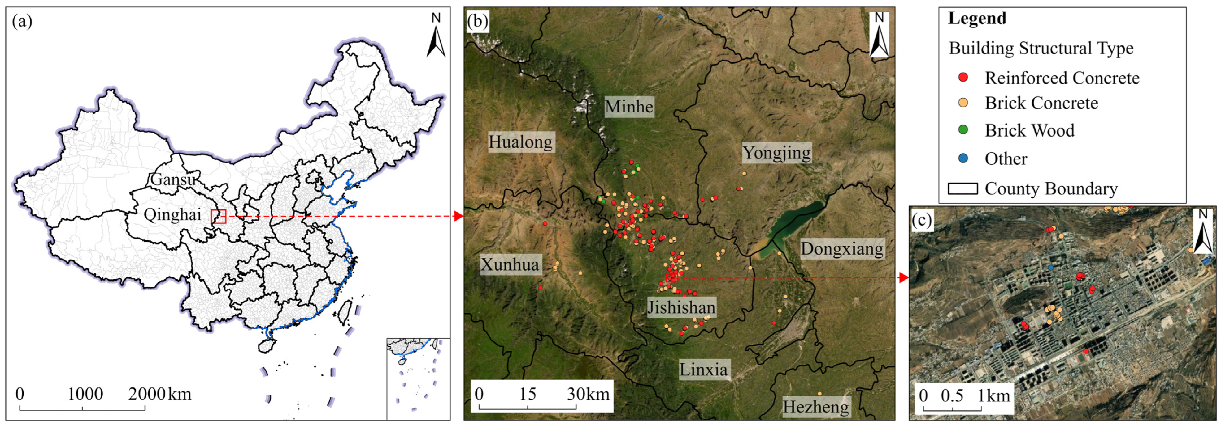
This study focuses on Linxia County, Yongjing County, Hezheng County and Jishishan County in Linxia, Gansu, and Xunhua County and Minhe County in Haidong, Qinghai (Figure 1). On 18 December 2023, a destructive earthquake (Ms 6.2) with an epicenter of 35.70°N and 102.79°E occurred in this region. The disaster was the most devastating in terms of casualties in China in 2023. Following the disaster, the National Disaster Reduction Center of China dispatched technical experts to the affected areas to conduct on-site investigations and collect post-earthquake building images. To further analyze the BSTs, the research team invited experts in relevant fields to interpret and annotate the BSTs in the images.

2.2. Study Data

2.2.1. Remote Sensing Data

The remote sensing data used in the research include optical images from Google Earth and SAR images from the GF3 satellite. The Google images have a spatial resolution of 0.6 m and include three spectral bands (Red, Green, Blue). These optical images correspond to pre-earthquake conditions and were selected for their very high spatial resolution, which allows for the extraction of shape, spectral, and texture features of different BSTs. The SAR images were downloaded from the National Cryosphere Desert Data Center (http://www.ncdc.ac.cn/) and have undergone post-processing such as radiometric calibration and geometric correction. The spatial resolution of the SAR images is 1 m.

2.2.2. Situ Data

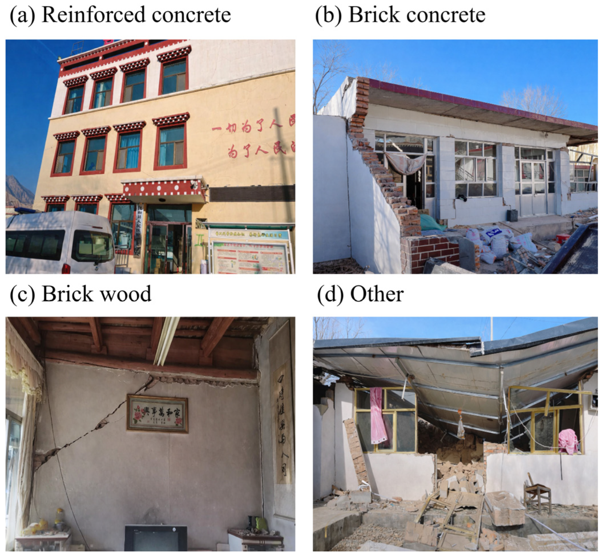
On 18 December 2023, a magnitude 6.2 earthquake struck Jishishan County in Linxia Prefecture, Gansu Province, causing severe structural damage to buildings. In the aftermath of the earthquake, the National Disaster Reduction Center of China dispatched technical experts to the affected areas to conduct on-site surveys and collect post-disaster building damage information. During the field investigation, high-resolution cameras were used to capture a total of 10,170 post-earthquake building images (Figure 2), with detailed annotations regarding the geographic location and damage status of each building. Furthermore, to facilitate structural analysis, experts in the relevant fields were invited to interpret and label each image individually, identifying the load-bearing structural types of the buildings.

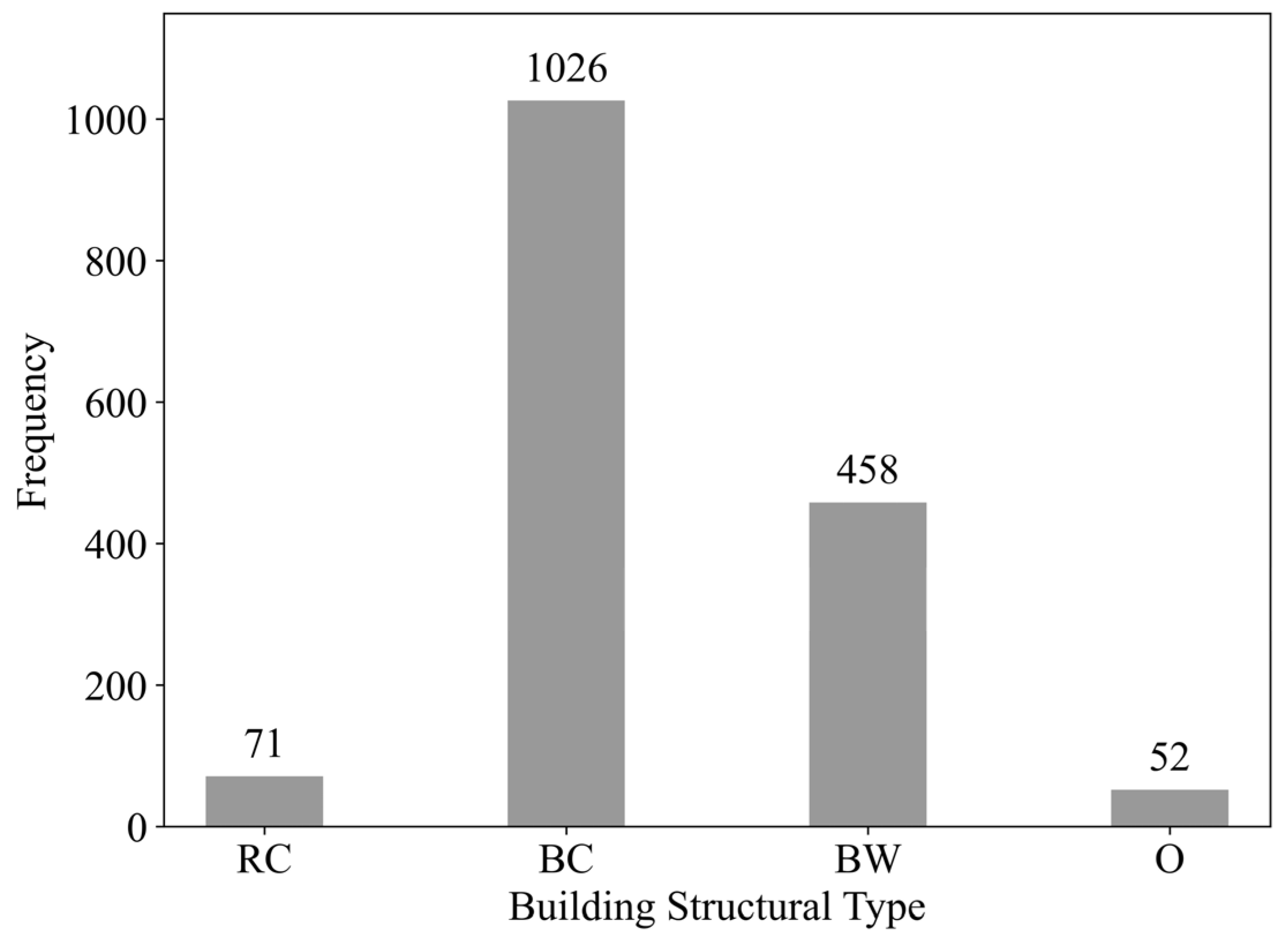
Experts then analyzed these images, marking the structural type and damage level of each building, resulting in 5976 validated checkpoints with effective BSTs. By comparing these checkpoints with remote sensing image data, the buildings at the checkpoints were digitized, and the structural types were annotated based on the load-bearing structure of the houses, categorized into the following types: reinforced concrete structure (RC), brick concrete structure (BC), brick wood structure (BW), and other structure (O) [17]. Due to the inaccuracies of GPS positioning, only 1607 buildings could be accurately assigned to corresponding building footprints on the remote sensing images, allowing for the extraction of geometric features based on the building vector data [13]. Figure 3 shows a histogram of different BSTs frequencies in the final field dataset.

2.2.3. Prior Knowledge Data

The distribution of BSTs is influenced not only by spectral, textural, and shape features derived from remote sensing imagery but also by various prior knowledge layers, including geographic, socioeconomic, and three-dimensional spatial attributes. First, the type of building structure is often associated with its distance from nearby roads. Previous studies have shown that buildings situated closer to roads are often newly constructed or renovated and thus tend to have better seismic performance and more robust structural types [18]. Therefore, in this study, we utilized multi-category road vector data provided by OpenStreetMap (OSM) to calculate the shortest distance from each building to different types of roads, such as highways, national roads, provincial roads, county roads, township roads, and residential roads. Second, topographic conditions play a crucial role in influencing the selection of BSTs. In areas with steep terrain, buildings are typically designed with more stable structural forms to withstand elevated disaster risks. To account for this, the study extracted elevation, slope, and aspect information from the DEM for each building location and incorporated these terrain factors into the analysis [19]. Additionally, BSTs are closely related to their three-dimensional characteristics, such as the number of floors and overall height [20]. To obtain building height data, we incorporated the nationwide building height dataset released by the National Earth System Science Data Center of China, which offers a spatial resolution of 10 m and is updated through 2020 [21]. However, due to the resolution mismatch between remote sensing imagery and the building height dataset, some buildings could not be directly matched with corresponding height values. To address this issue, we applied the Inverse Distance Weighting (IDW) interpolation method to fill in the missing values, thereby improving the completeness and spatial consistency of the three-dimensional building features. Finally, socioeconomic indicators also provide important complementary information for characterizing the spatial heterogeneity of BSTs. Macroscopic variables such as population, GDP, and nighttime light intensity reflect regional development level and human activity intensity, and previous studies have demonstrated that these factors are significantly associated with the distribution of BSTs [22]. In particular, regions with higher economic development levels generally exhibit larger residential floor areas and a higher proportion of RC buildings [23]. Therefore, these indicators are incorporated as auxiliary variables to enrich the feature space and enhance the stability and reliability of BST discrimination.

The spatial resolutions, data sources, and detailed descriptions of these heterogeneous multisource datasets are summarized in

Table 1. The database for the used data in this study.

Data Name	Spatial Resolution	Data Source
Optical images	0.6 m	Google Earth
GF3	1 m	National Cryosphere Desert Data Center (http://www.ncdc.ac.cn/)
Situ data	--	National Disaster Reduction Center of China
OSM	--	OpenStreetMap (https://www.openstreetmap.org/)
DEM	30 m	ASTER Global Digital Elevation Model (https://www.earthdata.nasa.gov/)
Population	1 km	LandScan (https://landscan.ornl.gov/)
GDP	1 km	Resource and Environmental Science Data Platform (https://www.resdc.cn/)
Nighttime Light [24]	500 m	NPP-VIIRS (https://doi.org/10.7910/DVN/YGIVCD) (accessed on 20 February 2025)
Building Height [21]	10 m	CNBH-10 m (https://zenodo.org/records/7064268#.YxtVAuxBz0p) (accessed on 19 March 2025)

. By integrating remote sensing image features with prior knowledge data, this study aims to comprehensively characterize the spatial distribution of BSTs, providing a richer and more accurate set of input features for subsequent building damage assessment and structural classification models.

3. Methods

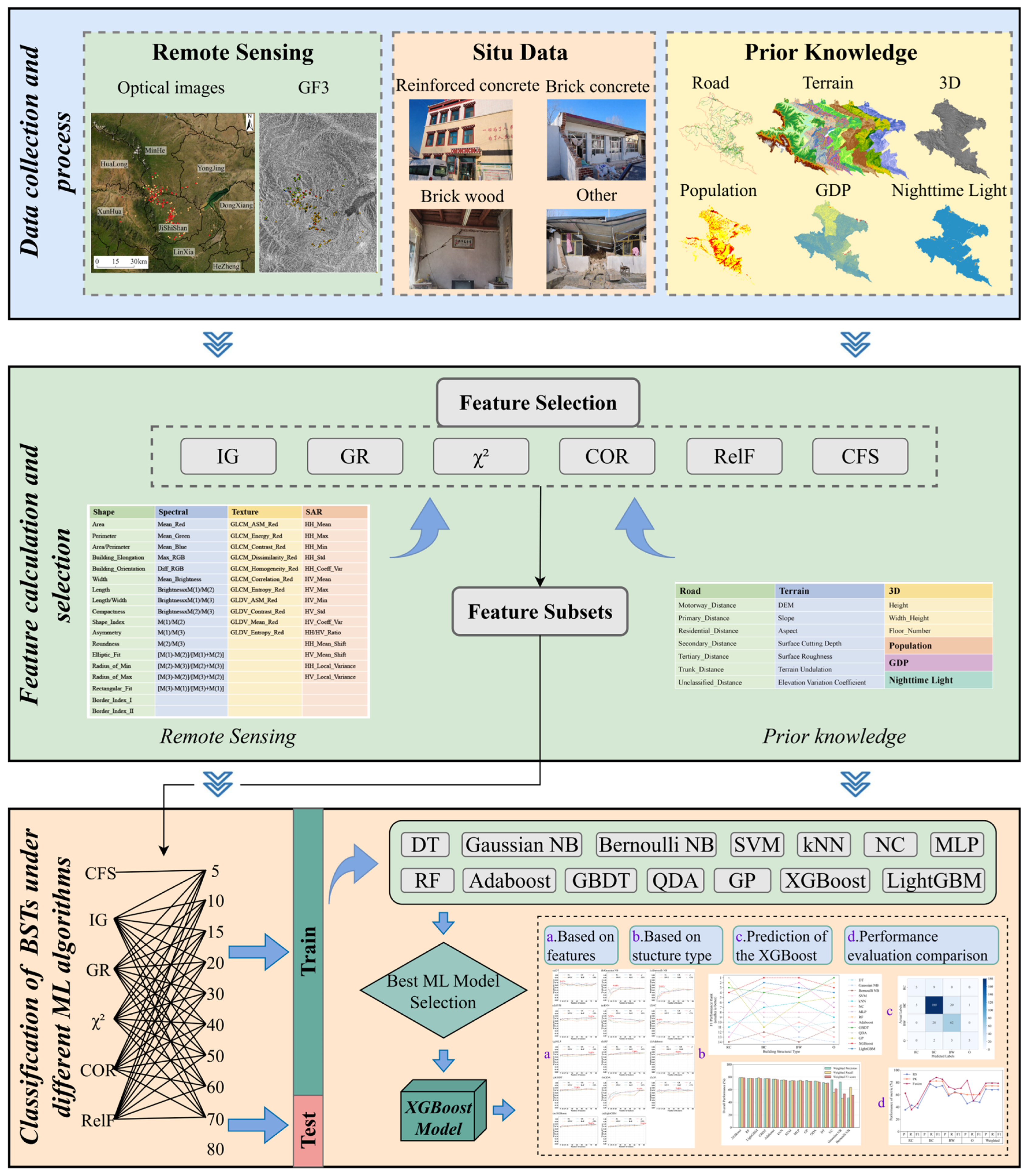
The research framework of this paper is as follows (Figure 4): First, high-resolution remote sensing imagery, prior knowledge data, and in situ data are collected and preprocessed to obtain relevant information for the study area. Then, based on these data, features are calculated from both remote sensing imagery and prior knowledge perspectives, and feature selection methods are applied to derive subsets of different feature combinations. Finally, these feature subsets are used as train and test data, input into 14 machine learning models for training and prediction. Based on a comparative evaluation of model performance, XGBoost (version 2.1.1) is ultimately selected as the most effective model for predicting BSTs.

3.1. Calculation of Building Features

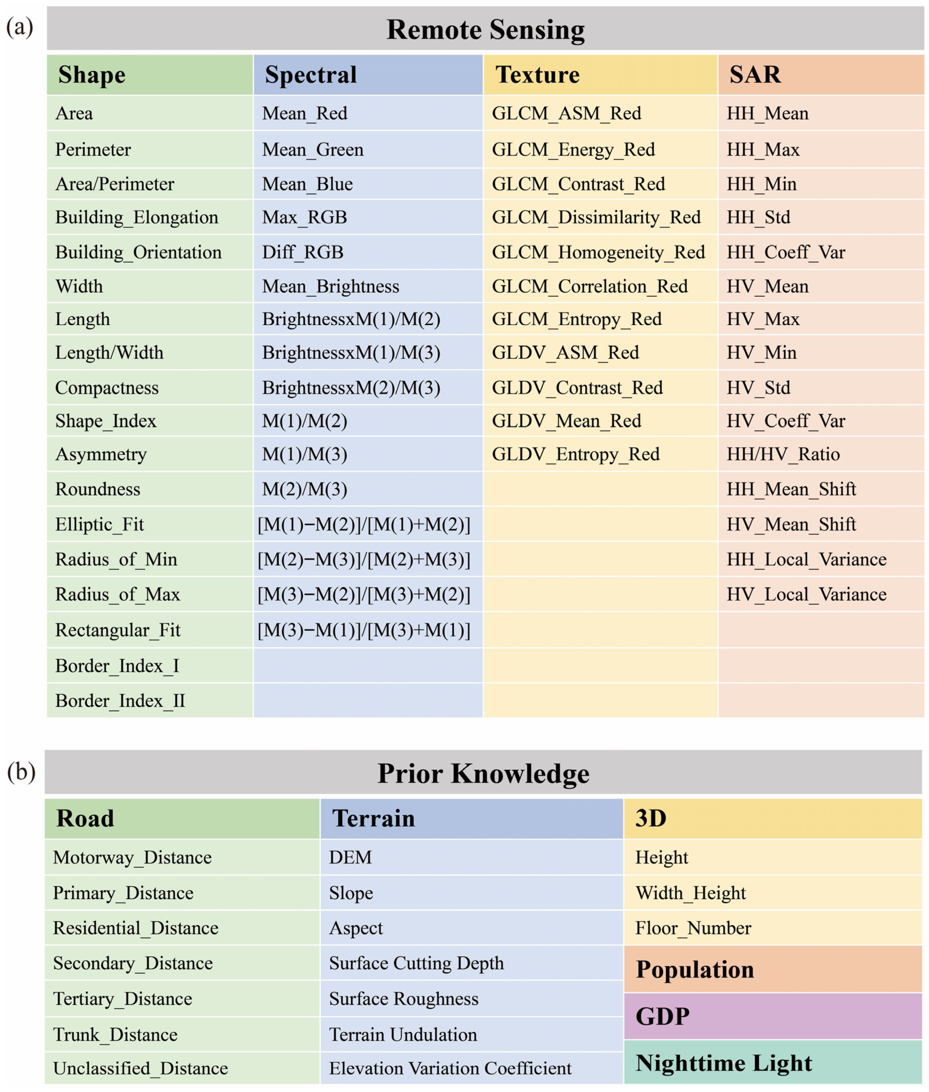
To more thoroughly assess BSTs, numerous features of each building are extracted from two major categories: remote sensing imagery and prior knowledge (Figure 5). We sequentially analyze and extract features related to BSTs from the aforementioned data sources. For remote sensing data, this includes shape features, spectral features, texture features and SAR features [7]. For optical image data, shape features of individual buildings such as Area, Perimeter, ratio of Area to Perimeter, Building Elongation, Building Orientation, Width, Length, ratio of Length to Width, Compactness, Shape Index, Asymmetry, Roundness, Elliptic Fit, Radius of Smallest Enclosing Ellipse, Radius of Largest Enclosing Ellipse, Rectangular Fit, Border Index I, and Border Index II are extracted. Additionally, spectral features of each pixel are extracted from the images, calculating the average, maximum, and brightness-related statistics for each band of the optical image, and averaging spectral features within each building area. Furthermore, texture features are represented by statistical values calculated using the Gray Level Co-occurrence Matrix (GLCM) and Gray Level Difference Vector (GLDV) [13]. For SAR imagery, features under HH and HV polarization are extracted, such as average, maximum, minimum, standard deviation, coefficient of variation, ratio of HH to HV, deviation from the mean, and variance. Detailed definitions and calculation formulas for all extracted features are provided in the Supplementary Materials [25,26,27].

And then, from the perspective of prior knowledge, for road data, the shortest distance of each building to various types of roads (motorway, trunk, primary, secondary, tertiary, unclassified, and residential) is calculated. For terrain data, slope, aspect, terrain ruggedness, ground roughness, surface cutting depth, and elevation coefficient of variation are calculated based on DEM data. For three-dimensional feature data, the 2020 CNBH Building Height Dataset was used to extract building height, width, and height-to-width ratio within the study area. Assuming a floor height of 3 m, the number of building floors was also estimated as a derived feature [28]. For population, GDP, nighttime light, and the above raster data, all layers were first unified in projection and then resampled to 0.6 m in ArcGIS 10.8.2 using the nearest neighbor method to ensure consistent grid alignment with the high-resolution imagery and to avoid introducing artificial interpolation. After grid alignment, zonal statistics were performed to calculate the mean value of each feature within each building footprint. All these features serve as independent variables, with BST as the dependent variable. Overall, each building object is represented by an 80-dimensional feature vector, and establishing relationships between these features and BSTs can effectively identify the BSTs in other areas. To ensure better model training, outliers in the above data were removed, and samples with NoData values in their features were excluded. As a result, 1589 buildings were retained as valid samples for analysis [14].

3.2. Classification of BSTs Based on Features

3.2.1. Feature Selection

Considering the high dimensionality of the input data, feature selection is necessary to reduce redundancy and computational cost, mitigate overfitting, and improve overall classification performance. The feature selection methods include filter method, wrapper method, and embedded method [29]. The filter method scores and ranks features directly based on the results of statistical tests or a specified criterion, selecting the top-ranked features [30]. The wrapper method selects features by creating different feature subsets and evaluating their performance using a predefined learning algorithm [31]. The embedded method involves training with certain machine learning algorithms and models, obtaining the weight coefficients for each feature, and selecting features based on their coefficients in descending order [32]. In our study, we have chosen the filter method for feature selection because it operates independently of the classifier, enabling us to distinguish between the effectiveness of algorithms for individual features and for feature subsets. Within the filter methods, we have selected six different filtering approaches, including Information Gain (IG), Gain Ratio (GR), Chi-squared (χ²), Spearman’s Rank Correlation Coefficient (SPCC), Relevance Feature (RelF), and Correlation-based Feature Selection (CFS) [13]. These methods were selected to capture complementary feature relevance criteria and improve the robustness of feature selection.

IG is a commonly used method for feature selection, mainly applied in decision tree algorithms, used to evaluate the amount of information that a feature provides about the target variable [33]. GR is a variation in IG that considers the intrinsic information of the feature, addressing the issue where IG tends to favor features with more values [34]. The χ² is a statistical test used to check the independence of two categorical variables. In feature selection, it is used to evaluate the association between a feature and the target variable [35]. The SPCC is a non-parametric statistical measure used to assess the strength of the monotonic relationship (either increasing or decreasing trend) between variables [36]. RelF is a method for measuring the correlation between features and the target class, typically based on some form of statistical association measure [34]. CFS is a method for evaluating the quality of feature subsets, considering not only the correlation between features and the target variable but also the redundancy among features, ultimately resulting in the best feature subset [37].

Figure 5. Features derived from remote sensing data and prior knowledge to characterize the BSTs.

Figure 5. Features derived from remote sensing data and prior knowledge to characterize the BSTs.

3.2.2. Oversampling for Handling Imbalanced Datasets

As shown in Figure 3, the distribution of BSTs is imbalanced, with a larger number of samples for brick concrete structures, while reinforced concrete structures and other types have significantly fewer samples. This imbalance in the dataset leads to machine learning models being biased towards the majority class, thus neglecting the minority class in terms of predictive performance. To address this issue, we applied SMOTE oversampling to the training data [38]. SMOTE (Synthetic Minority Over-sampling Technique) is a widely used oversampling technique that increases the number of minority class samples through synthetic sample generation, aiming to achieve class balance and improve the model’s generalization capability [39]. Unlike simply replicating minority class samples, SMOTE introduces sample diversity by generating synthetic samples, which helps the model generalize better on unseen data. For each sample in the minority class, the SMOTE algorithm randomly selects samples from its k-nearest neighbors. For the selected minority class sample and its randomly chosen neighbor, SMOTE generates new sample feature values by interpolating between the feature vectors of the original sample and the selected neighbor. Oversampling was applied only to the minority class samples, without sampling the majority class, until the number of samples in each class was approximately equal. This approach helps improve the model’s ability to distinguish various BSTs while maintaining data diversity.

In this study, SMOTE is used to alleviate class imbalance and support classifier training, rather than to generate physically realistic building samples. It should be noted that the feature space used in this study is heterogeneous and consists of remote sensing features and prior knowledge variables. As a result, synthetic samples generated through interpolation may not strictly correspond to physically interpretable building conditions. Therefore, SMOTE is employed solely as a methodological strategy to support classifier training and decision boundary learning, rather than for physical inference. Oversampling is restricted to the training set, and the independent test set contains exclusively real observations.

3.2.3. Machine Learning Algorithm Selection

Since there is no single best machine learning algorithm across different fields and applications, this study selected and tested 14 popular machine learning model algorithms based on the characteristics of limited sample sizes and high-dimensional features. To ensure a fair and reproducible comparison among different classifiers, hyperparameters for all models were systematically optimized using grid search combined with cross-validation implemented in Python 3.9.12 (scikit-learn 1.2.2, XGBoost 2.1.1). For each algorithm, a predefined hyperparameter search space was explored, and the optimal configuration was selected based on cross-validation performance on the training set. The detailed hyperparameter ranges for all 14 algorithms are provided in Supplementary Table S1. These algorithms include Decision Tree (DT) [40], Naïve Bayes (NB, including both Gaussian and Bernoulli variants) [41], Support Vector Machines (SVM) [42], k-Nearest Neighbors (kNN) [43], Nearest Centroid (NC) [44], Multi-Layer Perceptron (MLP) [45], Random Forest (RF) [46], Adaboost [47], Gradient Boosted Decision Tree (GBDT) [48], Quadratic Discriminant Analysis (QDA) [49], Gaussian Process (GP) [50], Extreme Gradient Boosting (XGBoost) [51], and Light Gradient Boosting Machine (LightGBM, version 4.5.0) [52]. These algorithms encompass a variety of learning strategies [53], including supervised learning and ensemble learning, aimed at exploring best model performance in cases where features are complex and sample sizes are limited. We divided the feature subsets obtained from six feature selection methods into training and testing sets in an 8:2 ratio, and then sequentially applied them to the aforementioned machine learning algorithms for model training and prediction, in order to compare the performance of different models and ultimately select the optimal one for BST recognition.

4. Results

4.1. Relevance of Features

The study adopted six methods for the optimal selection of high-dimensional features. Among them, IG, GR, χ², and SPCC are bivariate techniques, where each feature is evaluated independently of all other features in the dataset. In contrast, RelF and CFS aim to identify optimal subsets of features by considering feature interactions. For the RelF method, multiple values of the number of nearest neighbors (k) were tested. Cross-validation was employed to evaluate the performance across different k values, ensuring that the selected features performed robustly on the training set. CFS selects the optimal feature subset based on the evaluation scores of feature subsets.

We rank feature importance using IG, GR, χ², and SPCC. Then, using the RelF, we determine the value of n for the feature subset. Based on this n value, we select n features in order of importance using the IG, GR, χ², and SPCC methods. Finally, machine learning models are trained on the feature subsets obtained from these six methods. The results of the feature selection algorithms were used to construct feature subsets for multiple multiclass classification models. Based on the results of each ranking method, eight subsets were created containing n “best ranked” features (n = 5, 10, 15, 20, 30, 40, 50, 60, 70) [13]. Additionally, a feature subset was constructed based on the results of the CFS technique (n = 5). In total, there are 47 datasets: one containing the original number of features and 46 representing the feature subsets.

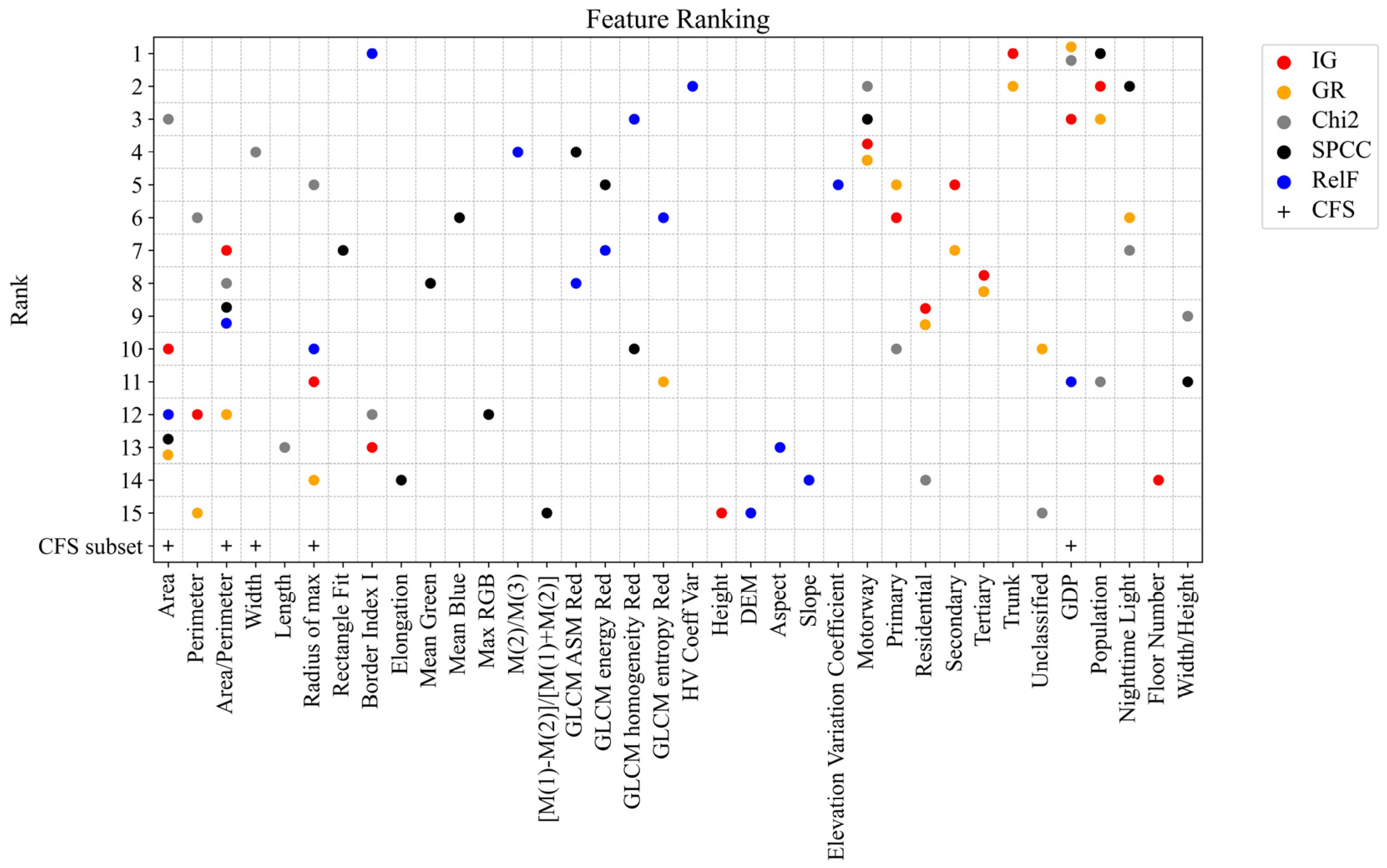
To select the most accurate feature combinations, we employed six feature selection methods: IG, GR, χ², SPCC, RelF, and CFS. To identify the most effective combination of features, six feature selection methods were employed to score each feature. Based on the importance reflected by these scores, the features were ranked accordingly. The top 15 ranked features, along with the feature subset selected by the CFS method, were ultimately chosen (Figure 6). Among the original 80-dimensional feature vector, a total of 36 features were included either in the ranking results or in the CFS subset. The results from multiple feature selection methods consistently indicate that socioeconomic variables such as GDP, nighttime light intensity, and population rank highly in feature importance, demonstrating strong and stable statistical relevance. In the study area, BSTs exhibit spatial differentiation at the regional scale. Although these variables have relatively coarse spatial resolution, they can capture regional-scale contrasts that are not always fully reflected by remote sensing features, including shape, spectral, textural, and SAR features, alone.

4.2. Performance Analysis of Different Machine Learning Algorithms

4.2.1. Based on Features

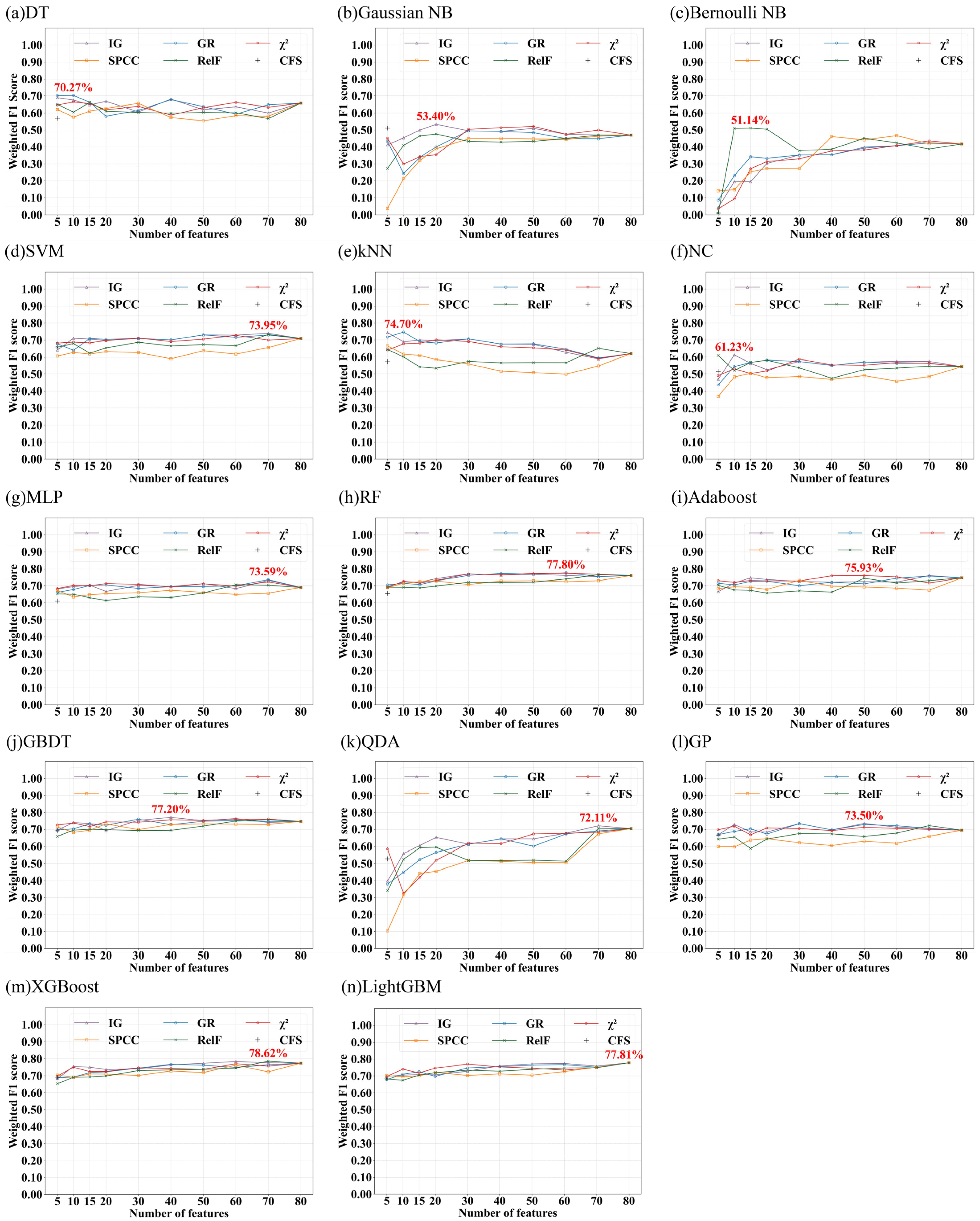
Based on the feature subsets constructed using the aforementioned feature selection methods, various machine learning algorithms were applied for classification. Their performance is evaluated using the weighted F1 score, which accounts for the imbalanced distribution of BSTs by weighting each class according to its sample proportion. The results are shown in Figure 7. As illustrated, XGBoost, LightGBM, RF, and GBDT achieved the highest overall performance, with weighted F1 score of 78.62%, 77.81%, 77.80%, and 77.20%, respectively. These results correspond to feature subsets consisting of the top 70 features selected by RelF for XGBoost, the full feature set of 80 features for LightGBM, the top 60 features selected by GR for RF, and the top 40 features selected by IG for GBDT. Among the 14 evaluated methods, these four tree-based models consistently exhibited superior and stable performance, with weighted F1 scores approaching 0.78.

Figure 6. The ranking of features under different feature selection methods.

Figure 6. The ranking of features under different feature selection methods.

4.2.2. Based on Structural Types

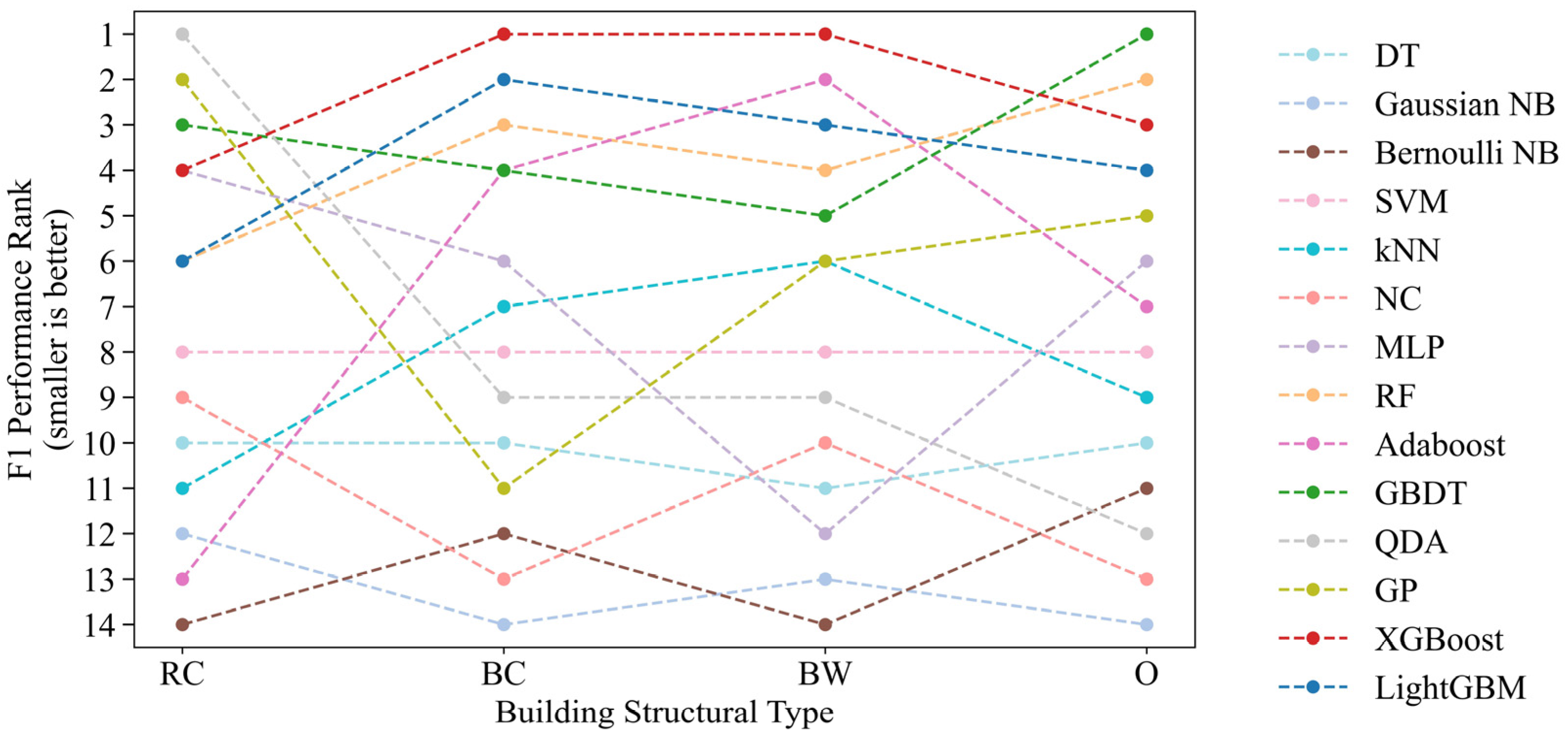
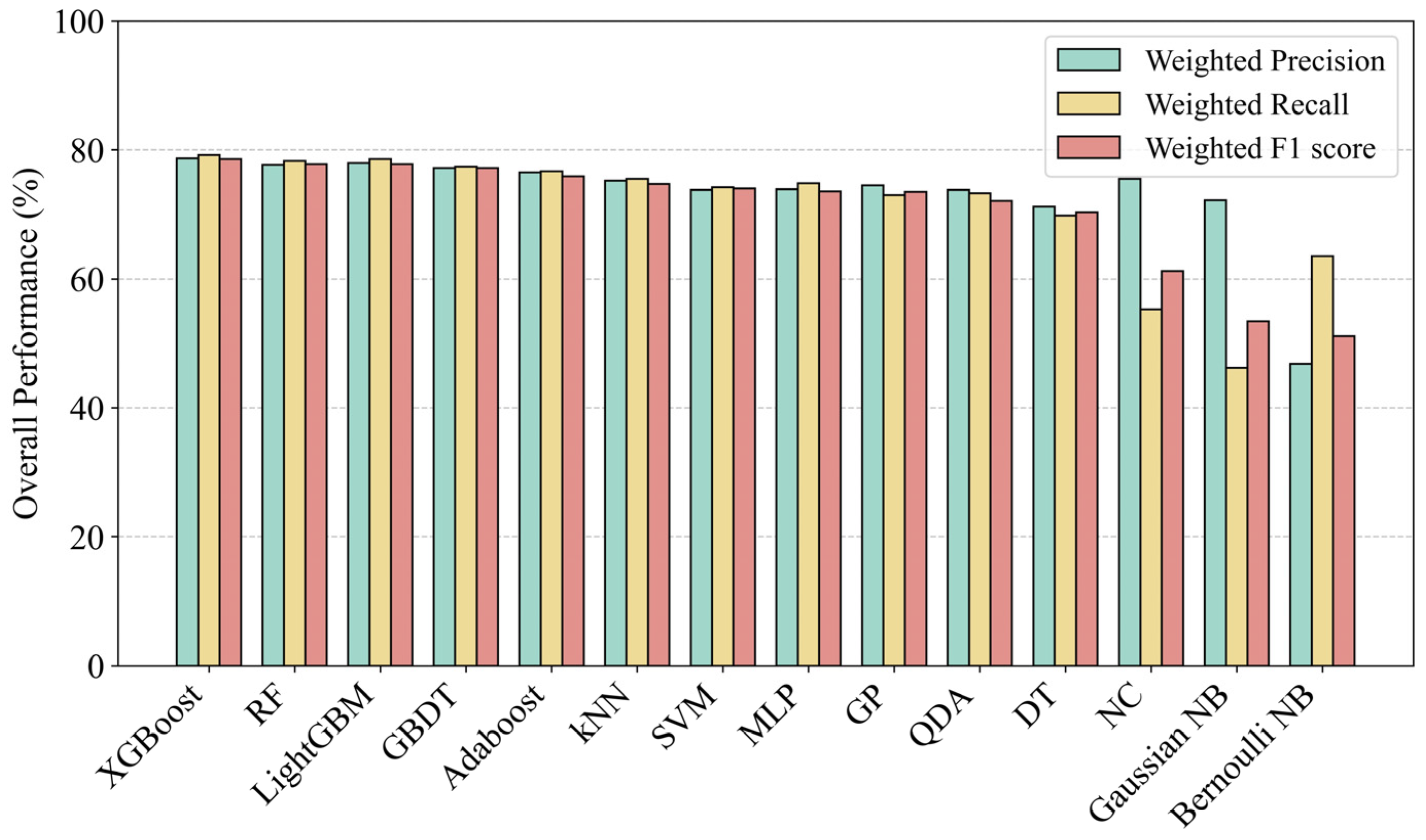
By classifying four BSTs, the 14 aforementioned machine learning methods were evaluated using precision, recall, and F1 score to assess the performance of each structure type, as well as using weighted precision, weighted recall, and weighted F1 score to evaluate the overall performance. The weighted metrics were computed as the weighted averages of class-wise metrics according to the sample proportions of each class.

Table 2. Best performance of each machine learning algorithm for each structure. ML—Machine learning; P—Precision; R—Recall; F1—F1 score.

ML	Performance per Structure												Overall Performance
	Reinforced Concrete			Brick Concrete			Brick Wood			Other			Weighted
	P	R	F1	P	R	F1	P	R	F1	P	R	F1	P	R	F1
DT	36.4	28.6	32.0	80.2	79.4	79.8	61.4	56.7	59.0	22.7	50.0	31.3	71.2	69.8	70.3
Gaussian NB	17.6	64.3	27.7	80.7	45.1	57.9	68.5	41.1	51.4	9.1	90.0	16.5	72.2	46.2	53.4
Bernoulli NB	100.0	7.1	13.3	64.4	97.5	77.6	0.0	0.0	0.0	33.3	20.0	25.0	46.8	63.5	51.1
SVM	38.5	35.7	37.0	80.5	82.8	81.6	66.7	64.4	65.5	50.0	40.0	44.4	73.8	74.2	74.0
kNN	60.0	21.4	31.6	79.6	86.3	82.8	71.8	62.2	66.7	35.7	50.0	41.7	75.2	75.5	74.7
NC	21.4	85.7	34.3	87.1	52.9	65.9	64.9	55.6	59.9	9.8	60.0	16.9	75.5	55.3	61.2
MLP	62.5	35.7	45.5	78.1	89.2	83.3	68.7	51.1	58.6	50.0	50.0	50.0	73.9	74.8	73.6
RF	45.5	35.7	40.0	81.7	87.7	84.6	72.8	65.6	69.0	85.7	60.0	70.6	77.7	78.3	77.8
Adaboost	33.3	21.4	26.1	81.7	85.3	83.5	68.8	71.1	69.9	100.0	30.0	46.2	76.5	76.7	75.9
GBDT	54.5	42.9	48.0	82.7	84.3	83.5	67.0	67.8	67.4	87.5	70.0	77.8	77.2	77.4	77.2
QDA	75.0	42.9	54.5	77.7	83.8	80.7	61.8	61.1	61.5	100.0	10.0	18.2	73.8	73.3	72.1
GP	42.9	64.3	51.4	82.4	76.0	79.1	64.6	68.9	66.7	46.2	60.0	52.2	74.5	73.0	73.5
XGBoost	62.5	35.7	45.5	82.2	88.2	85.1	72.9	68.9	70.9	83.3	50.0	62.5	78.7	79.2	78.6
LightGBM	66.7	28.6	40.0	81.8	88.2	84.9	71.8	67.8	69.7	71.4	50.0	58.8	78.0	78.6	77.8
Average	51.2	39.3	37.6	80.1	80.5	79.3	63.0	57.3	59.7	56.1	49.3	43.7	-	-	-
Standard deviation	22.1	20.4	11.2	5.0	14.3	7.9	18.5	18.5	18.1	32.0	20.2	20.0	-	-	-

summarizes the best performance of all machine learning algorithms by structural types. Figure 8 presents the F1 performance of different machine learning algorithms for each structure. Figure 9 shows the overall performance of the machine learning algorithms.

Firstly, according to the F1 ranking of each method under different structures, XGBoost, LightGBM, RF, and GBDT have better comprehensive performance (Figure 8). XGBoost, LightGBM, RF, and GBDT performed relatively better, with weighted F1 scores of 78.6%, 77.8%, 77.8%, and 77.2%, respectively (Table 2). This is because they are all decision tree models, capable of handling high-dimensional data and the nonlinear relationships between complex features [54]. Moreover, RF is an ensemble learning method based on Bagging [55], while GBDT, XGBoost, and LightGBM are based on Boosting [56]. These methods are capable of capturing complex patterns, thereby improving overall classification performance. In addition, they handle class imbalance effectively, leading to more balanced performance across different classes, particularly for minority categories.

Secondly, reinforced concrete structures are the most difficult building type to classify. Table 2 shows that the average F1 score for RC is the lowest (37.6%). Even the highest F1 scores provided by XGBoost, and LightGBM are only slightly above 42.0%. Other structures are also relatively difficult to classify, with an average F1 of 43.4%, and the highest F1 scores under GBDT, and XGBoost are just above 77.0%. In contrast, brick concrete and brick wood structures exhibit more favorable average F1 scores (76.7% and 58.8%), with brick concrete being easier to classify. The F1 scores for brick concrete under XGBoost, and LightGBM are relatively the highest, exceeding 84%.

Figure 7. The performances of 14 machine learning models as a function of different feature sets. The feature sets were constructed based on the feature selection techniques described in Section 3.2.1. The x-axis lists the number of features included in each respective feature set, while the y-axis shows the weighted F1 score of the learning models.

Figure 7. The performances of 14 machine learning models as a function of different feature sets. The feature sets were constructed based on the feature selection techniques described in Section 3.2.1. The x-axis lists the number of features included in each respective feature set, while the y-axis shows the weighted F1 score of the learning models.

Thirdly, the proposed method demonstrates good applicability in BST recognition, with XGBoost, LightGBM, RF, and GBDT in particular achieving promising classification results. These machine learning algorithms achieved over 77% in weighted precision, weighted recall, and weighted F1 score for overall performance (Table 2). Due to the issue of class imbalance (with fewer samples for reinforced concrete and other structure), the weighted F1 score is the most appropriate evaluation metric, as it reflects the overall performance of the model across different categories, with particular emphasis on the prediction of smaller classes. As shown in Figure 9, XGBoost, LightGBM, RF, and GBDT model achieved high weighted F1 scores. Combined with feature-based model prediction accuracy, we chose XGBoost to apply to the first 70 feature subsets selected based on RelF test for prediction.

Figure 8. F1 performance rank of various machine learning algorithms for each structure. RC—Reinforced concrete; BC—Brick concrete; BW—Brick wood; O—Other.

Figure 8. F1 performance rank of various machine learning algorithms for each structure. RC—Reinforced concrete; BC—Brick concrete; BW—Brick wood; O—Other.

Figure 9. Comparison of machine learning algorithms’ overall performance by F1 in decreasing order.

Figure 9. Comparison of machine learning algorithms’ overall performance by F1 in decreasing order.

4.3. Prediction and Error Analysis of the Best Machine Learning Algorithms

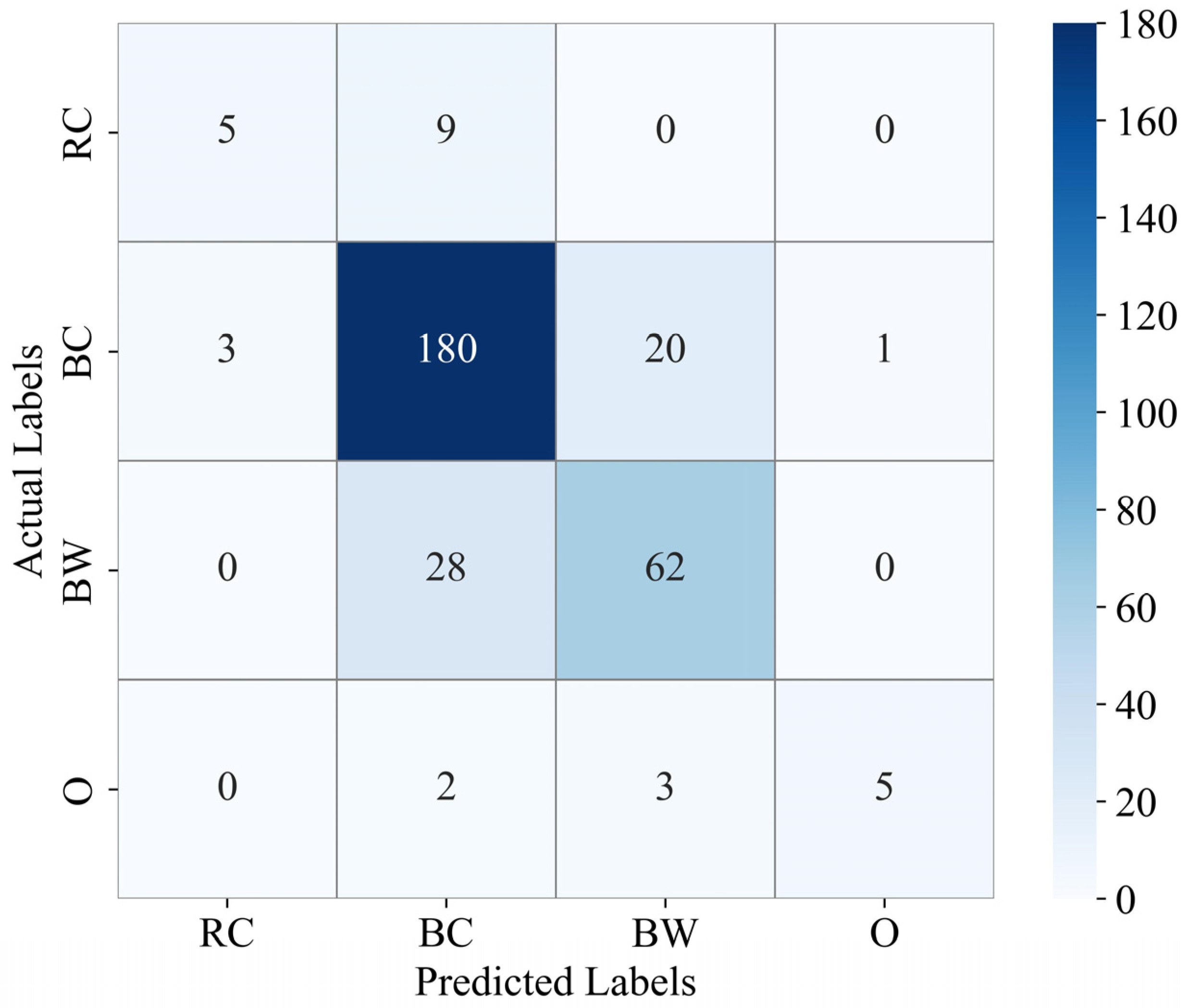
Since XGBoost was identified as the best-performing machine learning algorithm, the RelF method with 70 selected features was used for prediction, followed by an error analysis. The confusion matrix in Figure 10 presents classification errors for each structural type. In this matrix, the diagonal cells indicate the number of correctly classified buildings. It can be observed that most misclassifications occur between brick concrete and brick wood, where 20 BC samples were predicted as BW and 28 BW samples were predicted as BC. In contrast, RC structures were often misclassified as BC, while only a small portion of the other category was incorrectly identified as BC or BW.

To establish a clearer linkage between misclassifications and specific feature groups, we conducted an ablation-based error analysis by progressively removing different feature subsets from the baseline feature set. The resulting per-class F1 scores and dominant misclassification patterns under different feature settings are summarized in

Table 3. Per-class and weighted F1 scores under different feature ablation settings. Each ablation setting is obtained by removing one feature group from the baseline feature set. Weighted F1 denotes the weighted F1 score, accounting for class imbalance. The socioeconomic feature group includes population, GDP, and nighttime light intensity. RC—Reinforced concrete; BC—Brick concrete; BW—Brick wood; O—Other.

Setting	Features	RC_F1	BC_F1	BW_F1	O_F1	Weighted F1
Baseline	70	45.5%	85.1%	70.9%	62.5%	78.6%
Baseline-Shape	53	45.5%	85.0%	69.3%	47.1%	77.7%
Baseline-Spectral	54	38.1%	82.2%	64.4%	70.6%	74.8%
Baseline-Texture	60	30.0%	84.2%	68.2%	62.5%	76.6%
Baseline-SAR	63	33.3%	82.0%	66.3%	47.1%	74.3%
Baseline-Road	64	37.0%	81.7%	63.2%	57.1%	73.7%
Baseline-Terrain	63	41.7%	83.5%	66.3%	75.0%	76.5%
Baseline-3D	68	40.0%	83.5%	66.7%	66.7%	76.3%
Baseline-Socioeconomic	67	28.6%	81.8%	65.1%	58.8%	74.0%

and

Table 4. Dominant misclassification patterns under different feature ablation settings. RC ↔ BC, BC ↔ BW, and O ↔ BC/BW represent mutual misclassifications between the corresponding structural types, where samples from either class are incorrectly predicted as the other. Each ablation setting is obtained by removing one feature group from the baseline feature set. RC—Reinforced concrete; BC—Brick concrete; BW—Brick wood; O—Other.

Setting	RC ↔ BC	BC ↔ BW	O ↔ BC/BW
Baseline	12	48	5
Baseline-Shape	13	52	7
Baseline-Spectral	14	60	6
Baseline-Texture	15	52	7
Baseline-SAR	12	61	8
Baseline-Road	14	61	6
Baseline-Terrain	15	53	5
Baseline-3D	14	52	7
Baseline-Socioeconomic	14	54	7

, respectively. The results indicate that the dominant misclassification between brick concrete and brick wood structures is strongly associated with the absence of spectral, SAR, and distance to road features. When these feature groups are removed, misclassifications between BC and BW structures increase most markedly, accompanied by a noticeable decrease in the classification performance of both classes (Table 3 and Table 4). This suggests that spectral reflectance characteristics, SAR backscattering information, and distance to road contextual features provide complementary cues for distinguishing structurally similar masonry buildings. In addition, confusion between reinforced concrete and brick concrete structures increases most noticeably when terrain and texture features are excluded, which is also reflected by a clear reduction in RC classification performance. This pattern is consistent with the physical characteristics of RC and BC buildings: RC structures generally exhibit more complex vertical structure and surface texture, whereas BC buildings are typically simpler in form. Terrain context and texture descriptors therefore contribute to stabilizing the discrimination between these two classes. Misclassifications involving other structures further increase when SAR features are removed and are also amplified by the exclusion of shape, texture, three-dimensional, and socioeconomic features. Correspondingly, the classification performance of the other class degrades across these ablation settings (Table 3). This indicates that separating heterogeneous other structures from RC, BC, and BW building types relies on the joint contribution of radar information, geometric descriptors, and contextual features, rather than any single feature group.

To provide an intuitive illustration of these dominant misclassification patterns,

Table 5. Representative misclassification patterns and associated feature groups. Representative cases are grouped according to dominant misclassification patterns observed in the confusion matrix of the best-performing model. The red boxes in the Google Earth images indicate the locations of the building outlines shown in the adjacent column. The associated feature groups summarize feature sets that are sensitive to each misclassification pattern, as identified by the ablation-based analysis. RC—Reinforced concrete; BC—Brick concrete; BW—Brick wood; O—Other.

Case No.	Building Outline	Google Earth Image	In Situ Photo	True Label	Predicted Label	Associated Feature Groups
1				RC	BC	Associated with texture and terrain features.
2				BC	RC
3				BC	BW	Associated with spectral, SAR, and distance to road features.
4				BW	BC
5				BW	O	Associated with SAR, shape, texture, three-dimensional, and socioeconomic features.
6				O	BC
7				O	BW

presents representative misclassified cases grouped by error type. The associated feature groups listed in the table summarize feature sets that are sensitive to each misclassification pattern, as identified by the ablation-based analysis, at the pattern level rather than explaining individual cases.

4.4. Performance Evaluation Comparison

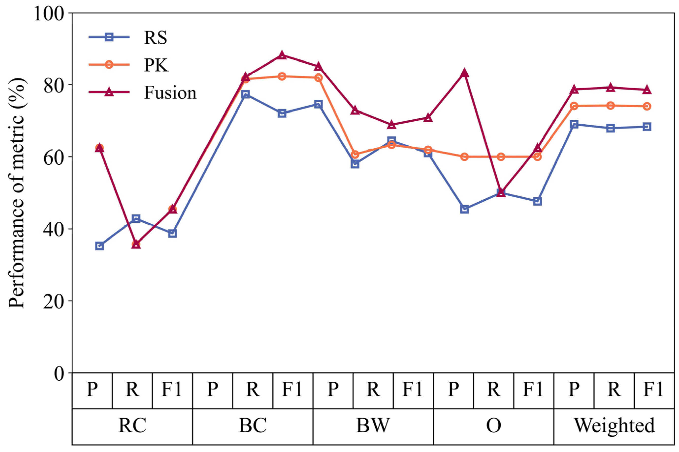
Figure 11 presents the classification performance of different structural types and weighted indicators under three feature configurations based on multisource remote sensing features and prior knowledge, combined with feature selection and machine learning methods:

(1)

Remote sensing features only, including shape, spectral, texture, and SAR features;

(2)

Prior knowledge features only, including road distance, terrain attributes, building height features, population, GDP, and nighttime light variables;

(3)

Fused features with feature selection, where all remote sensing and prior knowledge features are jointly integrated and the top 70 features selected by the RelF method are retained for model training.

The results indicate that models trained using remote sensing features or prior knowledge alone, even with the same machine learning model, do not achieve performance comparable to that of the fused feature set with feature selection. This demonstrates that the effective integration of multisource remote sensing features and prior knowledge, together with appropriate feature selection, significantly enhances BST recognition performance.

5. Discussion

5.1. Regional Heterogeneity and Generalization Limits

The BST identification model was primarily trained and validated using data from the 2023 Jishishan earthquake. When applied to other regions, its generalization capability may be constrained by pronounced regional heterogeneity in building materials, construction practices, and structural systems. Such regional differences can lead to shifts in feature distributions and limit the transferability of learned structural patterns, resulting in reduced recognition performance in unfamiliar contexts. This limitation highlights the importance of incorporating regionally diverse samples when developing generalized BST classification models. Future research should focus on constructing multi regional building structural databases that integrate representative structural characteristics from different geographic and socioeconomic contexts, thereby improving cross regional robustness and transferability.

5.2. Validation Constraints Under Post-Earthquake Conditions

Another limitation of this study lies in the constraints of validation data in post-earthquake environments. Although expert interpreted post-earthquake imagery was used to label BSTs, large scale and standardized ground truth datasets for BSTs remain scarce in real post-disaster scenarios. This limitation restricts systematic assessment of model uncertainty and hinders comprehensive evaluation under operational conditions. The lack of authoritative and consistently validated structural labels is a common challenge in post-earthquake research. Future studies could improve validation robustness by integrating multiple complementary data sources, such as expert interpretation, governmental construction records, and targeted field investigations, to establish higher quality reference datasets for selected regions.

5.3. Effects of Structural Type Imbalance on Classification Performance

The distribution of BSTs in post-earthquake samples is inherently imbalanced, reflecting the actual damage patterns associated with different construction systems. In the Jishishan earthquake dataset, damaged buildings were dominated by brick concrete and brick wood structures, while reinforced concrete buildings accounted for a smaller proportion. This structural type imbalance poses challenges for model training and evaluation, particularly for minority classes. Although SMOTE was employed to alleviate class imbalance during training, synthetic samples cannot fully capture the structural diversity of real buildings, which constrains classification performance for underrepresented structural types. This limitation reflects the combined effects of real world damage distributions and limited sample availability rather than methodological bias. Future work should aim to expand labeled samples across multiple earthquake events to improve representation of diverse structural types and enhance model robustness.

5.4. Methodological Considerations and Future Directions

This study adopts a feature-based machine learning framework that emphasizes robustness and interpretability under limited and imbalanced labeled samples. While recent advances in deep learning have demonstrated strong potential for automatic feature extraction from high-resolution imagery, their application in post-earthquake BST recognition remains challenging due to data scarcity and the need to integrate heterogeneous object level prior knowledge. Future research may explore hybrid frameworks that combine deep learning feature extraction with multisource prior knowledge, particularly as larger and more balanced labeled datasets become available. Such approaches may further enhance representation capacity while maintaining interpretability, thereby extending the applicability of BST recognition models in complex post-earthquake contexts.

6. Conclusions

This study aims to demonstrate how the integration of multisource remote sensing data and prior knowledge can be used to identify BSTs in earthquake scenarios, as well as to select the optimal machine learning model to verify the effectiveness of this integration. Since there is no significant direct correlation between raster pixel values and BSTs, obtaining a meaningful and discriminative feature set is essential for reliable classification. The main contribution of this study lies in the systematic incorporation of multidimensional prior knowledge to complement conventional remote sensing features, explicitly addressing the insufficient structural discriminative capability of image data in BST identification. The study utilizes high-resolution remote sensing imagery and various prior knowledge datasets, evaluating the classification performance of each feature set using different machine learning models and feature selection methods. The results indicate that, after feature selection and systematic model comparison, XGBoost trained on the top 70 features selected by the RelF method achieves the best overall performance (weighted F1 score = 78.62%). Further analyses reveal that different groups of remote sensing features and prior knowledge are associated with reductions in misclassification between specific BSTs. Compared with approaches relying solely on remote sensing imagery, the proposed feature fusion framework achieves higher and more balanced classification performance across different BSTs. In particular, the integration of multisource features leads to notable improvements for structure categories that are difficult to distinguish using single-source remote sensing features alone. Overall, this study demonstrates that combining prior knowledge with remote sensing features provides a more reliable representation of building structural characteristics, offering a practical reference for future BST identification studies in complex urban environments.

References

1. Allali, S.A.; Abed, M.; Mebarki, A. Post-Earthquake Assessment of Buildings Damage Using Fuzzy Logic. Eng. Struct. 2018, 166, 117–127. [Google Scholar] [CrossRef] [Scilit]
2. Fan, Y.; Wen, Q.; Wang, W.; Wang, P.; Li, L.; Zhang, P. Quantifying Disaster Physical Damage Using Remote Sensing Data—A Technical Work Flow and Case Study of the 2014 Ludian Earthquake in China. Int. J. Disaster Risk Sci. 2017, 8, 471–488. [Google Scholar] [CrossRef] [Scilit]
3. Wu, W.; Liu, X.; Zhou, Y.; Zhao, K. Spatial Heterogeneity of Built Environment’s Impact on Urban Vitality Using Multi-Source Big Data and MGWR. Sci. Rep. 2025, 15, 23459. [Google Scholar] [CrossRef] [Scilit]
4. Li, X.; Yang, Y.; Sun, C.; Fan, Y. Investigation, Evaluation, and Dynamic Monitoring of Traditional Chinese Village Buildings Based on Unmanned Aerial Vehicle Images and Deep Learning Methods. Sustainability 2024, 16, 8954. [Google Scholar] [CrossRef] [Scilit]
5. Tronin, A.A. Satellite Remote Sensing in Seismology. A Review. Remote Sens. 2010, 2, 124–150. [Google Scholar] [CrossRef] [Scilit]
6. An, J.; Nie, G.; Hu, B. Area-Wide Estimation of Seismic Building Structural Types in Rural Areas by Using Decision Tree and Local Knowledge in Combination. Int. J. Disaster Risk Reduct. 2021, 60, 102320. [Google Scholar] [CrossRef] [Scilit]
7. Zhou, Y.; Tan, Y.; Wen, Q.; Wang, W.; Li, L.; Li, Z. Deep Multimodal Fusion Model for Building Structural Type Recognition Using Multisource Remote Sensing Images and Building-Related Knowledge. IEEE J. Sel. Top. Appl. Earth Obs. Remote Sens. 2023, 16, 9646–9660. [Google Scholar] [CrossRef] [Scilit]
8. Rocchini, D. Effects of Spatial and Spectral Resolution in Estimating Ecosystem α-Diversity by Satellite Imagery. Remote Sens. Environ. 2007, 111, 423–434. [Google Scholar] [CrossRef] [Scilit]
9. Chen, C.; Yuan, X.; Gan, S.; Kang, X.; Luo, W.; Li, R.; Bi, R.; Gao, S. A New Strategy Based on Multi-Source Remote Sensing Data for Improving the Accuracy of Land Use/Cover Change Classification. Sci. Rep. 2024, 14, 26855. [Google Scholar] [CrossRef] [Scilit]
10. Momeny, M.; Latif, A.M.; Agha Sarram, M.; Sheikhpour, R.; Zhang, Y.D. A Noise Robust Convolutional Neural Network for Image Classification. Results Eng. 2021, 10, 100225. [Google Scholar] [CrossRef] [Scilit]
11. Xin, D.; Daniell, J.E.; Wenzel, F. Review Article: Review of Fragility Analyses for Major Building Types in China with New Implications for Intensity–PGA Relation Development. Nat. Hazards Earth Syst. Sci. 2020, 20, 643–672. [Google Scholar] [CrossRef] [Scilit]
12. Du, H.; Cao, Y.; Zhang, F.; Lv, J.; Deng, S.; Lu, Y.; He, S.; Zhang, Y.; Yu, Q. A Classification Method of Building Structures Based on Multi-Feature Fusion of UAV Remote Sensing Images. Earthq. Res. Adv. 2021, 1, 100069. [Google Scholar] [CrossRef] [Scilit]
13. Geiß, C.; Aravena Pelizari, P.; Marconcini, M.; Sengara, W.; Edwards, M.; Lakes, T.; Taubenböck, H. Estimation of Seismic Building Structural Types Using Multi-Sensor Remote Sensing and Machine Learning Techniques. ISPRS J. Photogramm. Remote Sens. 2015, 104, 175–188. [Google Scholar] [CrossRef] [Scilit]
14. Zhou, P.; Chang, Y. Automated Classification of Building Structures for Urban Built Environment Identification Using Machine Learning. J. Build. Eng. 2021, 43, 103008. [Google Scholar] [CrossRef] [Scilit]
15. Li, Z.; He, W.; Li, J.; Zhang, H. Identifying Every Building’s Function in Large-Scale Urban Areas with Multi-Modality Remote-Sensing Data. In IGARSS 2024—2024 IEEE International Geoscience and Remote Sensing Symposium; IEEE: New York, NY, USA, 2024; pp. 310–314. [Google Scholar]
16. Ren, D.; Qiu, X.; An, Z. A Multi-Source Data-Driven Analysis of Building Functional Classification and Its Relationship with Population Distribution. Remote Sens. 2024, 16, 4492. [Google Scholar] [CrossRef] [Scilit]
17. Ministry of Emergency Management of the People’s Republic of China. Statistical Survey System for Particularly Major Natural Disaster Losses; Ministry of Emergency Management: Beijing, China, 2020.
18. Atwal, K.S.; Anderson, T.; Pfoser, D.; Züfle, A. Predicting Building Types Using OpenStreetMap. Sci. Rep. 2022, 12, 19976. [Google Scholar] [CrossRef] [Scilit]
19. Zeng, G.; Zhao, D.; Chen, X.; Wang, X. Architectural Design Methods for Mountainous Environments. J. Asian Archit. Build. Eng. 2023, 22, 2596–2612. [Google Scholar] [CrossRef] [Scilit]
20. Lu, Z.; Im, J.; Rhee, J.; Hodgson, M. Building Type Classification Using Spatial and Landscape Attributes Derived from LiDAR Remote Sensing Data. Landsc. Urban Plan. 2014, 130, 134–148. [Google Scholar] [CrossRef] [Scilit]
21. Wu, W.-B.; Ma, J.; Banzhaf, E.; Meadows, M.E.; Yu, Z.-W.; Guo, F.-X.; Sengupta, D.; Cai, X.-X.; Zhao, B. A First Chinese Building Height Estimate at 10 m Resolution (CNBH-10 m) Using Multi-Source Earth Observations and Machine Learning. Remote Sens. Environ. 2023, 291, 113578. [Google Scholar] [CrossRef] [Scilit]
22. Gunasekera, R.; Ishizawa, O.; Aubrecht, C.; Blankespoor, B.; Murray, S.; Pomonis, A.; Daniell, J. Developing an Adaptive Global Exposure Model to Support the Generation of Country Disaster Risk Profiles. Earth-Sci. Rev. 2015, 150, 594–608. [Google Scholar] [CrossRef] [Scilit]
23. Marinova, S.; Deetman, S.; van der Voet, E.; Daioglou, V. Global Construction Materials Database and Stock Analysis of Res-idential Buildings between 1970-2050. J. Clean. Prod. 2020, 247, 119146. [Google Scholar] [CrossRef] [Scilit]
24. Chen, Z.; Yu, B.; Yang, C.; Zhou, Y.; Yao, S.; Qian, X.; Wang, C.; Wu, B.; Wu, J.; Liao, L.; et al. The Global NPP-VIIRS-like Nighttime Light Data (Version 2) for 1992–2024. Harv. Dataverse 2020, 304. [Google Scholar] [CrossRef] [Scilit]
25. Liuzzi, M.; Aravena Pelizari, P.; Geiß, C.; Masi, A.; Tramutoli, V.; Taubenböck, H. A Transferable Remote Sensing Approach to Classify Building Structural Types for Seismic Risk Analyses: The Case of Val d’Agri Area (Italy). Bull Earthq. Eng 2019, 17, 4825–4853. [Google Scholar] [CrossRef] [Scilit]
26. Haralick, R.M.; Shanmugam, K.; Dinstein, I. Textural Features for Image Classification. IEEE Trans. Syst. Man Cybern. 1973, SMC-3, 610–621. [Google Scholar] [CrossRef] [Scilit]
27. Weszka, J.S.; Dyer, C.R.; Rosenfeld, A. A Comparative Study of Texture Measures for Terrain Classification. IEEE Trans. Syst. Man Cybern. 1976, SMC-6, 269–285. [Google Scholar] [CrossRef] [Scilit]
28. Huang, H.; Chen, P.; Xu, X.; Liu, C.; Wang, J.; Liu, C.; Clinton, N.; Gong, P. Estimating Building Height in China from ALOS AW3D30. ISPRS J. Photogramm. Remote Sens. 2022, 185, 146–157. [Google Scholar] [CrossRef] [Scilit]
29. Kaur, A.; Guleria, K.; Kumar Trivedi, N. Feature Selection in Machine Learning: Methods and Comparison. In 2021 International Conference on Advance Computing and Innovative Technologies in Engineering (ICACITE); IEEE: New York, NY, USA, 2021; pp. 789–795. [Google Scholar]
30. Hancer, E.; Xue, B.; Zhang, M. Differential Evolution for Filter Feature Selection Based on Information Theory and Feature Ranking. Knowl.-Based Syst. 2018, 140, 103–119. [Google Scholar] [CrossRef] [Scilit]
31. Kohavi, R.; John, G.H. Wrappers for Feature Subset Selection. Artif. Intell. 1997, 97, 273–324. [Google Scholar] [CrossRef] [Scilit]
32. N, T.R.; Gupta, R. An Efficient Feature Subset Selection Approach for Machine Learning. Multimed. Tools Appl. 2021, 80, 12737–12830. [Google Scholar] [CrossRef] [Scilit]
33. Guyon, I.; Nikravesh, M.; Gunn, S.; Zadeh, L.A. (Eds.) Feature Extraction: Foundations and Applications; Studies in Fuzziness and Soft Computing; Springer: Berlin/Heidelberg, Germany, 2006; Volume 207. [Google Scholar]
34. Cai, J.; Luo, J.; Wang, S.; Yang, S. Feature Selection in Machine Learning: A New Perspective. Neurocomputing 2018, 300, 70–79. [Google Scholar] [CrossRef] [Scilit]
35. Sarra, R.R.; Dinar, A.M.; Mohammed, M.A.; Abdulkareem, K.H. Enhanced Heart Disease Prediction Based on Machine Learning and Χ2 Statistical Optimal Feature Selection Model. Designs 2022, 6, 87. [Google Scholar] [CrossRef] [Scilit]
36. Zar, J.H. Significance Testing of the Spearman Rank Correlation Coefficient. J. Am. Stat. Assoc. 1972, 67, 578–580. [Google Scholar] [CrossRef]
37. Theng, D.; Bhoyar, K.K. Feature Selection Techniques for Machine Learning: A Survey of More than Two Decades of Research. Knowl. Inf. Syst. 2024, 66, 1575–1637. [Google Scholar] [CrossRef] [Scilit]
38. Mujahid, M.; Kına, E.; Rustam, F.; Villar, M.G.; Alvarado, E.S.; De La Torre Diez, I.; Ashraf, I. Data Oversampling and Imbalanced Datasets: An Investigation of Performance for Machine Learning and Feature Engineering. J. Big Data 2024, 11, 87. [Google Scholar] [CrossRef] [Scilit]
39. Chawla, N.V.; Bowyer, K.W.; Hall, L.O.; Kegelmeyer, W.P. SMOTE: Synthetic Minority Over-Sampling Technique. J. Artif. Intell. Res. 2002, 16, 321–357. [Google Scholar] [CrossRef] [Scilit]
40. Quinlan, J.R. Induction of Decision Trees. Mach. Learn. 1986, 1, 81–106. [Google Scholar] [CrossRef] [Scilit]
41. Domingos, P.; Pazzani, M. On the Optimality of the Simple Bayesian Classifier under Zero-One Loss. Mach. Learn. 1997, 29, 103–130. [Google Scholar] [CrossRef] [Scilit]
42. Cortes, C.; Vapnik, V. Support-Vector Networks. Mach. Learn. 1995, 20, 273–297. [Google Scholar] [CrossRef] [Scilit]
43. Cover, T.; Hart, P. Nearest Neighbor Pattern Classification. IEEE Trans. Inf. Theory 1967, 13, 21–27. [Google Scholar] [CrossRef] [Scilit]
44. Tibshirani, R.; Hastie, T.; Narasimhan, B.; Chu, G. Diagnosis of Multiple Cancer Types by Shrunken Centroids of Gene Expression. Proc. Natl. Acad. Sci. USA 2002, 99, 6567–6572. [Google Scholar] [CrossRef] [Scilit]
45. Rumelhart, D.E.; Hinton, G.E.; Williams, R.J. Learning Representations by Back-Propagating Errors. Nature 1986, 323, 533–536. [Google Scholar] [CrossRef] [Scilit]
46. Breiman, L. Random Forests. Mach. Learn. 2001, 45, 5–32. [Google Scholar] [CrossRef] [Scilit]
47. Freund, Y.; Schapire, R.E. A Decision-Theoretic Generalization of On-Line Learning and an Application to Boosting. J. Comput. Syst. Sci. 1997, 55, 119–139. [Google Scholar] [CrossRef] [Scilit]
48. Friedman, J.H. Greedy Function Approximation: A Gradient Boosting Machine. Ann. Statist. 2001, 29, 1189–1232. [Google Scholar] [CrossRef] [Scilit]
49. Fisher, R.A. The Use of Multiple Measurements in Taxonomic Problems. Ann. Eugen. 1936, 7, 179–188. [Google Scholar] [CrossRef] [Scilit]
50. Rasmussen, C.E.; Williams, C.K.I. Gaussian Processes for Machine Learning. Int. J. Neural Syst. 2004, 14, 69–106. [Google Scholar] [CrossRef] [Scilit]
51. Chen, T.; Guestrin, C. XGBoost: A Scalable Tree Boosting System. In Proceedings of the 22nd ACM SIGKDD International Conference on Knowledge Discovery and Data Mining 2016; ACM: New York, NY, USA, 2016; pp. 785–794. [Google Scholar] [CrossRef] [Scilit]
52. Ke, G.; Meng, Q.; Finley, T.; Wang, T.; Chen, W.; Ma, W.; Ye, Q.; Liu, T.-Y. LightGBM: A Highly Efficient Gradient Boosting Decision Tree. Adv. Neural Inf. Process. Syst. 2017, 30, 52. [Google Scholar]
53. Ganaie, M.A.; Hu, M.; Malik, A.K.; Tanveer, M.; Suganthan, P.N. Ensemble Deep Learning: A Review. Eng. Appl. Artif. Intell. 2022, 115, 105151. [Google Scholar] [CrossRef] [Scilit]
54. Costa, V.G.; Pedreira, C.E. Recent Advances in Decision Trees: An Updated Survey. Artif. Intell. Rev. 2023, 56, 4765–4800. [Google Scholar] [CrossRef] [Scilit]
55. Altman, N.; Krzywinski, M. Ensemble Methods: Bagging and Random Forests. Nat. Methods 2017, 14, 933–934. [Google Scholar] [CrossRef] [Scilit]
56. Bentéjac, C.; Csörgő, A.; Martínez-Muñoz, G. A Comparative Analysis of Gradient Boosting Algorithms. Artif. Intell. Rev. 2021, 54, 1937–1967. [Google Scholar] [CrossRef] [Scilit]
Figure 1. Overview of the study area and spatial distribution of BSTs. (a) National location of the study area within China. (b) Regional distribution of building samples by structural type across the study area, overlaid on a satellite basemap. (c) Zoomed-in view of a selected local area (highlighted by the red box in panel (b)), illustrating the detailed spatial distribution of different BSTs.
Remotesensing 18 00597 g001
Figure 2. Photographs taken on site following the Jishishan earthquake.
Remotesensing 18 00597 g002
Figure 3. Frequency of labeled samples (overall: 1607) according to different BSTs in situ data. RC—Reinforced concrete; BC—Brick concrete; BW—Brick wood; O—Other.
Remotesensing 18 00597 g003
Figure 4. The research framework. Arrows indicate the workflow sequence. Different colors are used only to distinguish feature categories.
Remotesensing 18 00597 g004
Figure 10. Confusion matrix for the best performing machine learning algorithm XGBoost. RC—Reinforced concrete; BC—Brick concrete; BW—Brick wood; O—Other.
Remotesensing 18 00597 g010
Figure 11. Comparison of BST recognition performance under three feature configurations. (1) remote sensing features only (RS); (2) prior knowledge features only (PK); and (3) fused features (Fusion) with RelF feature selection (top 70 features). P—Precision; R—Recall; F1—F1 score. RC—Reinforced concrete; BC—Brick concrete; BW—Brick wood; O—Other.
Remotesensing 18 00597 g011