Airborne Laser Scanning for Large-Scale Forest Carbon Quantification: A Comparison of LiDAR Single-Tree and Field-Based Methods

Highlights

What are the main findings?

• Airborne laser scanning (ALS) can produce carbon estimates that are broadly comparable to those of traditional field-based inventories.
• The traditional plot-based quantifications better accounted for dead tree carbon, but ALS better accounted for live tree carbon in sparse forested conditions.

What are the implications of the main findings

• The future use of remote sensing, especially ALS, for carbon quantifications looks promising.
• Hybrid or adjusted inventory approaches may be necessary in dense or mortality-rich forests.

Abstract

This study evaluated airborne laser scanning (ALS) as a large-scale tool for forest carbon quantification by comparing ALS-derived estimates with traditional field sampling across multiple forest strata. Above-ground biomass was estimated using two different, commonly used equations, while below-ground biomass was derived from peer-reviewed root-to-shoot ratios. ALS and field estimates differed across forest strata and carbon pools: ALS detected higher live tree carbon in harvested areas—capturing residual trees often missed in traditional cruises—but underestimated dead wood carbon, relative to field-based methods. Consistent differences were also observed between biomass equations, with Woodall estimates being 12.8% and 16.7% lower than Jenkins estimates for ALS and field methods, respectively. The study further incorporated soil organic carbon (SOC) and carbon dating data, providing additional insight into subsurface carbon stocks and the temporal dynamics of forest carbon pools. Overall, ALS proved to be an efficient, repeatable, and scalable method for carbon assessment, offering clear advantages in monitoring carbon flux over time when integrated with forest management protocols. Although further research is needed to refine biomass equations and explore emerging technologies such as Geiger Mode LiDAR, ALS has strong potential to enhance forest carbon crediting processes and support climate change mitigation goals.

1. Introduction

Climate change constitutes a significant societal challenge, prompting strategies aimed at reducing greenhouse gas emissions and minimizing carbon footprints. Among these strategies, forest carbon credits—simply defined as units of additional biogenic carbon stored in forests to offset emissions generated elsewhere—have gained traction as an effective mechanism for facilitating climate change mitigation, particularly when on-site reductions are either physically or economically impractical.

Terrestrial forests play a vital role in a variety of carbon credit-generating pathways because they facilitate the capture of atmospheric carbon through the process of photosynthesis and its conversion into biomass. Nature-based forest-dependent carbon dioxide removal (CDR) solutions typically involve the active management of forests to increase carbon stocks in the form of above- and below-ground woody biomass, as well as soil organic carbon (SOC). These solutions may include the intentional manipulation of ecosystems, particularly in disturbed or degraded areas, to restore ecological functions and increase carbon sequestration. Within carbon registries, these kinds of forest management CDR projects take the form of afforestation, reforestation, or revegetation (ARR), in which trees are planted in areas that have been deforested in the past or have never been forested, and improved forest management (IFM), in which existing forests are managed to promote tree growth and carbon sequestration, rather than maximizing the net present value through intensive timber harvest. When forests are part of managed systems that sustainably harvest biomass for products (e.g., timber, paper, energy), carbon- or CO₂-bearing waste streams from those processes may also become part of additional CDR pathways in the form of biochar or sequestered CO₂. These are sometimes referred to as biomass carbon removal and storage or BiCRS approaches [1], because the sequestered carbon is biogenic and hence provides a net drawdown of atmospheric CO₂ when considered on a full life-cycle basis.

The demand for high-quality nature-based CDR is anticipated to grow exponentially [2]. This increasing interest highlights the necessity for enhanced standardization and transparency in carbon quantification methodologies [3]. Central to the scalability of forest-based CDR is the precise quantification of forest carbon pools during the establishment of a project (e.g., baseline) and periodic remeasurement. Protocols established by carbon registries, such as the California Air Resources Board (ARB), the American Carbon Registry (ACR), the Verified Carbon Standard (VCS), and the Gold Standard for the Global Goals (Gold Standard) currently mandate on-site sampling, typically in the form of permanent monitoring plots, to develop these inventories [4,5,6,7]. Compared to stand-based forest inventories conducted for timber sales or land valuation, carbon inventories are typically performed at a larger scale, commonly at the strata or property level, and exhibit a lower tolerance for error to ensure the accuracy of estimated carbon stocks. This precision enhances the confidence and legitimacy of carbon credits within the framework of climate change mitigation objectives. One key challenge to this reduced error tolerance is the fact that many regions and countries do not have accurate biomass or carbon estimates. This necessitates reliance on summaries from institutions like the Intergovernmental Panel on Climate Change [8] and/or the need for on-site data collection exercises. Accurately mapping forest structures that account for forest heterogeneity, growth and loss cycles, carbon flux, topography, and the wide range of global management practices make carbon and biomass accounting a challenging monitoring prospect [9].

For nearly a century, traditional sample-based forest inventory methods have been common practice in forestry and are widely accepted for carbon and biomass estimation in registry methodologies. These methods use a smaller subset of trees to impute estimates across large areas. However, data collection is inherently labor-intensive and costly, particularly with regard to travel expenditure [10,11], and design and sampling error rates need to be considered when evaluating results. Such errors can emanate from various sources, including omission of ecological considerations, inclusion of non-representative sample locations, inadequate sample sizes, improper plot type selection, and/or poor stratification [12,13,14]. Measurement errors can also be common during ground-based inventory data collections [12,15], and can be made worse when multiple individuals, with varying levels of experience, are involved in data collection. If not addressed, these data challenges can manifest as failed audits or verifications, often slowing or halting project timelines.

Current sample-based biomass, carbon stock, and carbon flux assessments differ based on the desired spatial and temporal scales. The eddy covariance (EC) method measures carbon fluxes through a network of flux towers that use a variety of sensors to make measurements [16]. The estimated net ecosystem exchange is defined as the gains and losses of carbon between soil, vegetation, and the atmosphere. These tower-based measurements are limited both by the number of towers within a given forest and the limited number of EC projects across representative biomes internationally. Another quantification method relies on standard provincial, national, and international inventories informed with sub-models and allometric relationships [17,18]. With increased insect outbreaks and wildfires, forest stands are in danger of shifting from carbon sinks to sources, resulting in potential inventory inaccuracies [19].

In recent years, advancements in light detection and ranging (LiDAR) technology and processing have improved the accuracy of alternative forest inventory workflows, some of which can produce near-census level products [20,21,22]. At the appropriate density and specifications, LiDAR data provide the ability to quantify detailed attributes of individual trees to accurately inform metrics such as height, count, diameter at breast height (DBH), and, ultimately, tree wood volume [23,24,25]. Because wood volume strongly correlates with stored carbon [26,27], LiDAR-based inventories may be a viable solution for large-scale forest carbon quantification.

LiDAR is an umbrella term that encompasses numerous technologies, including terrestrial laser scanning (TLS), mobile laser scanning (MLS), and airborne laser scanning (ALS) [28]. It is worth noting that some LiDAR technologies may be less suited to the large-scale data collection that is typically required for forest carbon quantification and monitoring projects. When considering factors such as time efficiency, cost-effectiveness, and data quality, ALS generally supersedes TLS and MLS as the approach that best scales detailed data collection for precise measurement of forest metrics, including those used to quantify forest carbon [29,30]. In recent years, several studies have confirmed that calibrating ALS with field data further decreases systematic biases, resulting in more robust and accurate outcomes [20,21,22,31,32].

Application of ALS across landscape scale geographies can result in significant reductions in project cost and duration when compared with conventional sampling methods [29]. The rapid and consistent acquisition of data over extensive areas further provides simultaneous measurement of additional non-timber forest resources, adding additional value to project and research efforts [30,33]. Time-efficient ALS collections mitigate the potential for temporal inconsistencies within data collections where field personnel capacity is limited by inaccessible, rugged, or hazardous terrain, ensuring robust coverage under diverse conditions [34,35]. Similar to precision agriculture, the adoption of ALS within forestry has begun with multiple organizations and landowners having to, or preparing to, re-structure their inventory and accounting systems to incorporate ALS-based products.

Carbon registries are increasingly supporting the incorporation of remote sensing data into forest carbon CDR project development, monitoring, and verification processes. Early versions of registry methodologies included no requirements for the incorporation of remote sensing data outside of its potential use for project boundary delineations [36,37]. Conversely, the most recent versions of registry methodologies (at the time of this publication) allow for the use of aerial or satellite imagery for baseline scenario determinations [38] and land use analyses for project eligibility determinations [39]. While such registry updates requiring remote sensing data analyses have focused on the use of satellite imagery, the new VCS VM0047 ARR methodology allows for the incorporation of ALS-derived canopy height models in dynamic performance benchmarking of planted areas against off-site baseline control plots [40].

As remote sensing technologies continue accruing more interest and responsibility in forest carbon initiatives, exploring the feasibility of ALS-based carbon quantification solutions is a logical next step. Simultaneously, understanding the accuracy and precision of biomass estimates from these solutions will be paramount in vetting their use in carbon crediting protocols. A central concern is the degree of flexibility that is inherent within existing protocols that promote selectively structuring projects to maximize profit, rather than greenhouse gas (GHG) reduction benefits [3]. One way for project proponents to avoid criticism may be to enhance transparency. The scalable, near-census nature of ALS-based carbon inventories may prove advantageous in this regard. Specific problems such as biasing carbon stock estimates by intentionally avoiding harvest of monitoring plots or claiming underestimated levels of leakage could potentially be reduced to non-factors. In the current protocols, 2+ year old management plans, a certification from an organization such as the Forest Stewardship Council (FSC) or Sustainable Forestry Initiative (SFI), or other documentation indicating reasonable harvest levels can be used by landowners to demonstrate no activity leakage beyond de minimis [5,38]. Unfortunately, none of these options provide hard evidence to inform true harvest levels. Complete coverage of repeat ALS inventories across ownership, in addition to the project area, may prove superior by transparently addressing the total change in carbon stocks to inform the actual harvest levels. Additionally, when repeat ALS acquisitions are available prior to project establishment, trends in biomass reductions due to harvest through time could easily be assessed to establish or validate baseline scenarios. Another, perhaps more obvious, benefit of multi-temporal ALS scans over the course of the project lifespan is the accurate quantification of carbon sequestration resulting from tree growth. Additionally, integrating ALS-derived data with other spatial information related to land use patterns, climatic trends, and biodiversity indicators may provide a more holistic understanding of forest ecosystems and offer deeper insights into the dynamics of carbon sequestration, leading to a more nuanced assessment of potential risks. Given these potential benefits, along with the growing demand for transparent, credible, and verifiable carbon crediting projects, it is reasonable to explore ALS as a valid option for forest landowners and project proponents. To do so, it is important to first evaluate how ALS-integrated methods compare with traditional carbon quantification approaches at the foundation of a forest carbon project—measuring the carbon itself. Motivated by these considerations, this study takes a practical approach to evaluating an existing ALS-based carbon quantification method and assessing how it compares with traditional field-based approaches endorsed by carbon credit registries in a diverse forested setting.

2. Materials and Methods

2.1. Subsection

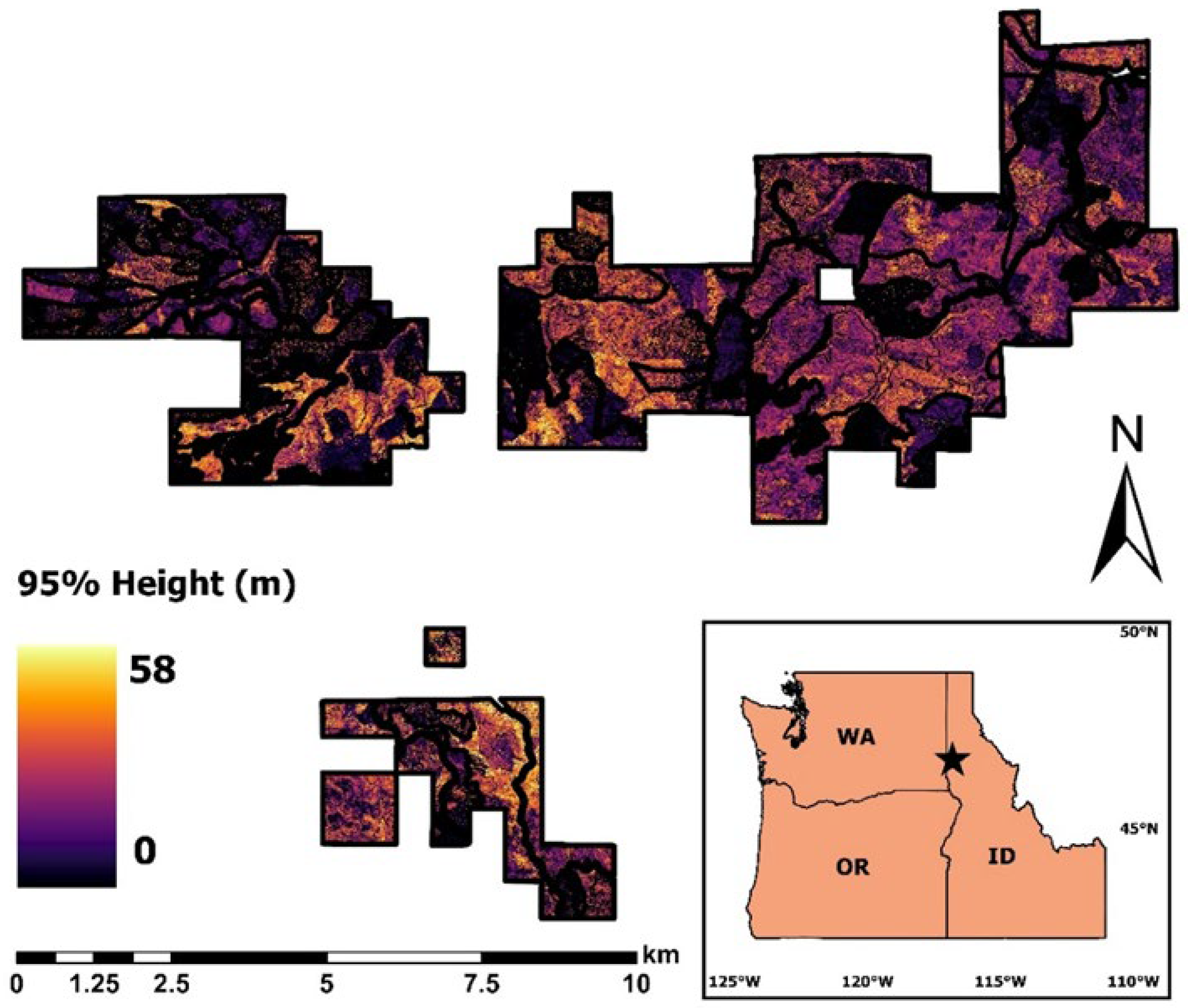
This study was conducted in the University of Idaho experimental forest (UIEF), located in the Palouse Range, approximately 20 km northeast of Moscow, Idaho USA (Figure 1). The UIEF is a temperate mixed conifer forest with various species compositions and age structures. Present tree species include Pseudotsuga menziesii (Mirb.) Franco var. glauca (Beissn.) Franco (Douglas fir), Abies grandis (Douglas ex D. Don) Lindl. (grand fir), Larix occidentalis Nutt. (western larch), Pinus ponderosa Dougl. ex Laws. (ponderosa pine), Pinus contorta Douglas ex Louden (lodgepole pine), Thuja plicata Donn ex D. Don (western redcedar), Pinus monticola var. minima Lemmon (western white pine), and Picea engelmannii var. glabra Goodman (Engelmann spruce). The UIEF is subject to active and ongoing management aimed at achieving multiple objectives, including the sustainable production of timber, the advancement of scientific research, and the facilitation of educational initiatives. Its substantial size and diverse forested landscapes made the UIEF an ideal testing ground for the concepts and technologies evaluated in this study.

2.2. Traditional Field Data Collection

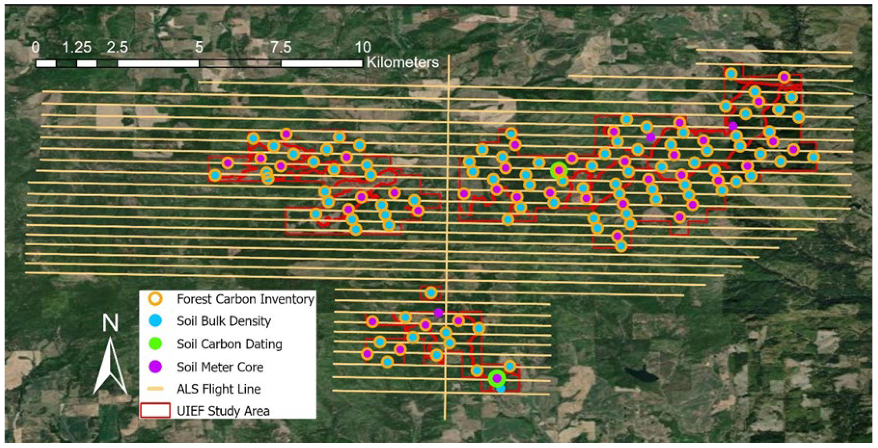
A traditional forest carbon inventory, compliant with standards set forth by ACR, ARB, Verra, and the BioCarbon Fund [4,5,7,41], using human-measured ground samples, was conducted for the study area in the summer of 2024. Prior to sampling, the study area was delineated into the following four strata by using aspect and historical forest inventory data: Douglas fir wet sites (DFW), Douglas fir dry sites (DFD), mixed conifer sites (MXC), and recently harvested sites (CC). Sample sizes for each stratum were informed by using the variability of existing plot data from previous inventories. Additionally, 1/10th acre fixed-radius sample plots containing a 1/100th acre nested regeneration plot were placed, using a systematic grid with 450 m spacing. The first grid point was placed randomly, and as a result, all subsequent points in the grid were also considered to be randomly placed. A 74.4 ft (2 plot radii) buffer was applied to strata boundaries and drivable roads within the study area. Plots within buffers were excluded from sampling to minimize edge effects. In total, 127 plots were measured across the four strata, yielding an overall sampling intensity of approximately 61 acres per plot (

Table 1. Size and forest inventory plot count of the project strata.

Stratum	Hectares	Plot Count	Tree Count
Harvested (CC)	635	22	88
Douglas fir dry (DFD)	211	9	183
Douglas fir wet (DFW)	700	32	928
Mixed conifer (MXC)	1571	64	1248
Total	3117	127	2447

, Figure 2).

Cruisers navigated to plot locations using Garmin GPSMAP 64sx (Garmin International, Inc., Olathe, KS, USA) global positioning system (GPS) units. Once at the plot, Javad Triumph 2 (Javad, San Jose, CA, USA) GPS units were used to determine the plot center. Plot centers were monumented by inserting a wooden stake into the ground, leaving four to six inches of the stake visible above the surface. Additionally, two to three foot-long orange ribbons were hung above (or as close as possible to) plot centers. Within each plot, data were recorded for all living and dead trees with a diameter at 4.5 feet (DBH) greater than or equal to one inch. Trees with a DBH greater than or equal to five inches were recorded in the 10th acre plot, whereas trees with a DBH of less than five inches were recorded in the nested 100th acre plot. Trees were measured in a clockwise fashion, beginning with the closest tree to the plot center, approximately due north. Paint was used to number the first tree at each plot, as well as an additional four trees in the cardinal directions. Recorded attributes for each tree included species, DBH, total height, and live/dead status. The location of DBH measurements were marked with white paint. Tools used to obtain measurements included a standard logger’s tape and a Haglöf laser (Haglöf Sweden, Långsele, Sweden). Following completion of the inventory, the data were used to quantify forest carbon stocks.

2.3. ALS Data Collection and Preprocessing

ALS data were acquired in July 2024, using a RIEGL VQ-1560II sensor [42] (RIEGL, Horn, Austria) mounted on a fixed-wing aircraft fitted with a Gyro Stabilization Mount [43] (SOMAG AG Jena, Jena, Germany). The aircraft maintained an altitude between 2000 and 2500 m above ground level, with flight lines flown in alternating orientations and a 50% overlap, relative to the sensor’s 58° field of view (Figure 2). Strata-level scan densities ranged from 33.2 to 36.7 pulses per square meter (PPM), with an overall average of approximately 36 PPM (

Table 2. Average pulse densities for project strata.

Stratum	Average Pulse Density (PPM)
CC	35.0
DFD	33.3
DFW	36.7
MXC	34.9

).

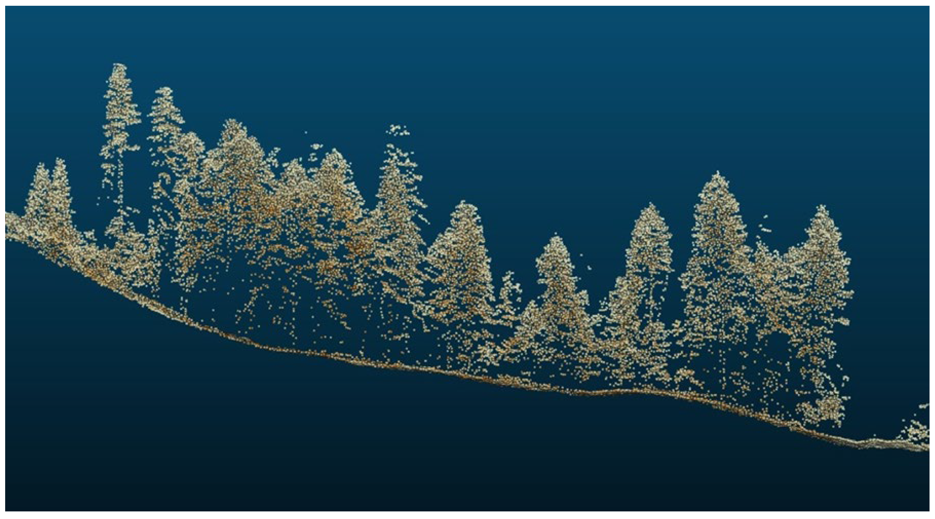
Over the forested area, an average pulse return rate of four was achieved (Figure 3). ALS returns were preprocessed to normalize laser intensity within the RIEGL RiPROCESS 1.9.4 software [44] (RIEGL, Horn, Austria) and classified to bare earth, vegetation, water, buildings, and noise, before being tiled into 500 m². LAZ file-type tiles by the LiDAR acquisition company were delivered to our team for processing.

2.4. ALS Individual Tree Detection and Measurement

The ForestView^® LiDAR processing pipeline developed by Northwest Management Incorporated was applied to ALS. LAZ files to detect individual tree objects and populate their metrics. The system first creates a digital elevation model (DEM) and digital surface model (DSM) directly from the ALS point cloud, both at 0.3 m resolution. These layers are then used to derive a canopy height model (CHM). Iterations of different algorithms (watershed, local maxima, etc.) [45,46] are then used to detect high points in the CHM, which are assumed to correspond with apices of tree objects. Such algorithms are proven to be well suited for identifying pyramidal or columnar coniferous crowns [22]. The location of each tree object is recorded as an XY coordinate and the corresponding CHM height value is assigned to the tree as the total tree height. From there, a comprehensive suite of more than 100 descriptive metrics is extracted and/or derived for each detected tree object. These metrics characterize multiple dimensions of the forest environment, including LiDAR-based structural properties of the segment (e.g., crown structure, crown volume, and crown area), local topography, canopy cover, climatic variables such as temperature and precipitation, and soil quality and related edaphic characteristics. A feature selection process is then applied to identify the most informative subset of metrics for modeling key tree attributes that are relevant to carbon quantification: primarily diameter at breast height (DBH), species, and live/dead status. The resulting predictor sets can be attribute-specific, such that the metrics selected to predict species can differ from those used to model tree status, for example. Additionally, the optimal predictors for a given modeled attribute can vary across geographic or regional contexts due to spatial heterogeneity in forest structure and environmental conditions. With predictor sets defined, preliminary predictions are generated using a range of modeling approaches, including parametric methods such as linear regression and nonparametric approaches, primarily machine learning models. Cross validation is heavily used during the modeling process to determine the best model fit. Bias correction, calibration, and validation are then performed using an internal database of locally stem-mapped trees with corresponding field measurements and ALS-derived observations, ensuring consistency between remotely sensed estimates and ground-based data. Additional details on ForestView^® processing, outputs, and performance in various forested conditions are reported in [20,21,22].

2.5. Traditional Tree Carbon Quantification

Because registry methodologies often differ in acceptable biomass calculation methodologies, two different published biomass approaches—Jenkins et al., 2003 [47] (Jenkins) and Woodall et al., 2011 [48] (Woodall)—were applied to the completed field inventory to derive gross estimates of above-ground tree biomass in kilograms for each measured tree in the study area. These methodologies are cited for use in forest carbon projects: specifically, Jenkins for ACR and both Jenkins and Woodall for VCS [38,49]. Required tree inputs for the Jenkins equations were species and DBH, whereas species, DBH, and total tree height were needed for the Woodall equations because the cubic foot volume is used to calculate bole biomass. The Jenkins equation for total above-ground tree biomass is shown below:

$$bm=Exp\left({\beta }_0+{\beta }_1\mathit{ln}DBH\right)$$

(1)

where bm is the total above-ground biomass (kg) for trees with a diameter equal to or greater than 2.5 cm at breast height, Exp is the exponential function, ${\beta }_0$ and ${\beta }_1$ are the species group-specific coefficients in [47], ln is the natural log base “e” (2.718282), and DBH is the diameter (cm) at breast height. To generate Woodall-derived estimates of above-ground tree biomass, Equations (1)–(10) in [48] were used (Appendix A). Stump oven dry biomass from [50] and sapling adjustment factors from [51] were included as inputs. All estimates of below-ground tree biomass were calculated using the component ratio method (CRM) that relies on equations developed by Jenkins and others [47]. All biomass equations, including CRM equations, are listed in Appendix A. Above and below-ground estimates were summed for each tree to produce the total tree estimates. The total tree estimates were then multiplied by the inverse of their corresponding plot size (10 for trees in the main plot and 100 for trees in the nested sub plot) to yield biomass per acre represented by each individual tree. Main and subplot biomass per acre values were then summed to a single plot-level biomass per acre estimate. The mean biomass per acre value across plots within each stratum was then multiplied by respective stratum acreage to calculate the total gross biomass for each stratum. To convert biomass to carbon, kilograms to metric tons, and carbon to CO₂e, gross stratum biomass estimates were multiplied by 0.5, divided by 1000, and multiplied by 3.664, respectively. Stratum MTCO₂e estimates were then summed to calculate the study area total. In addition, 80 percent confidence intervals were calculated at the strata and project levels using the following:

$$CI=\overline{x}\pm t\left({\displaystyle \frac{s}{\sqrt{n}}}\right)$$

(2)

where CI is the confidence interval, $\overline{x}$ is the sample mean, t is the critical value of a t-distribution, s is the sample standard deviation, and n is the number of sample plots.

2.6. ALS-Based Tree Carbon Quantification

The same above and below-ground biomass estimation methodologies [47,48] were applied to each tree in the ALS-informed inventory, using ForestView^®-generated tree metrics such as height, diameter, and species to calculate gross estimates of total tree biomass in kilograms. Stratum level estimates of gross biomass were calculated by summing gross tree biomass estimates within each stratum. To convert biomass to carbon, kilograms to metric tons, and carbon to CO₂e, gross stratum biomass estimates were multiplied by 0.5, divided by 1000, and multiplied by 3.664, respectively. Stratum MTCO₂e estimates were then summed to calculate the total study area estimate.

2.7. Soil Organic Carbon (SOC)

To determine SOC stocks, 132 soil cores were extracted throughout the project area consisting of 88 0–30 cm depth sample locations and 44 m core sample locations (Figure 2); samples were split into 0–15, 15–30, 30–60, and 60–100 cm layers. All samples for carbon and bulk density analysis were packaged and shipped to Trace Genomics for analysis and quantification. Two additional meter cores were collected for carbon dating analysis to address soil carbon sequestration rates over time. These samples were shipped to Beta Analytics for analysis. Soil organic carbon stock densities were calculated at each sample site, using the following:

$${SOC}_i=C_i\ast h_i\ast p_i$$

(3)

where SOC_i is the estimated soil carbon per area for depth layer i, C_i is the soil organic carbon concentration, h_i is the length of the depth layer, and p_i is the fine mass (course fragments removed) soil bulk density. Stocks were summed by depth layer at the project level and for each stratum, then divided by the corresponding number of samples to obtain mean estimates. Additionally, margins of error at 90% confidence were calculated.

2.8. Comparison of Estimates

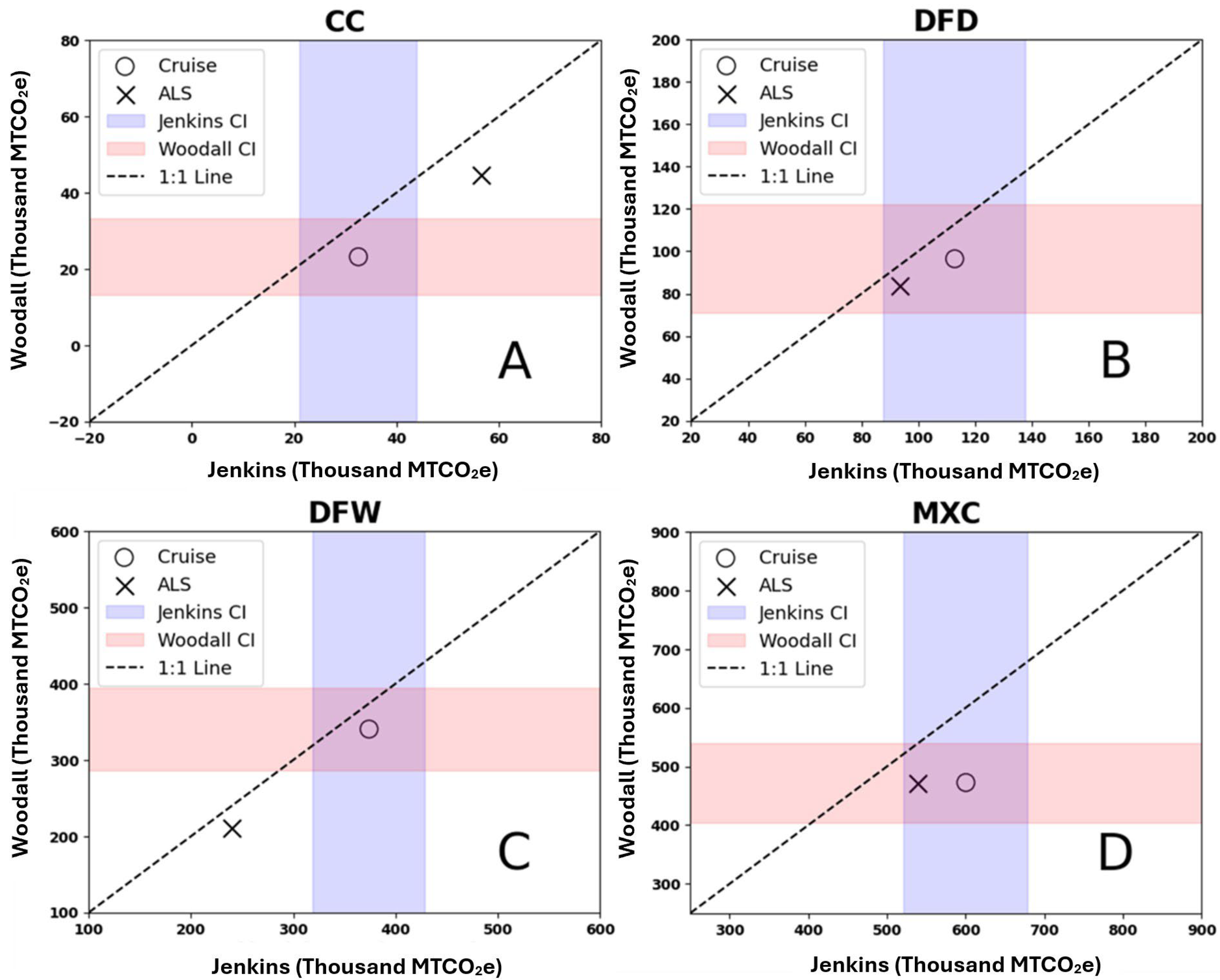
Strata and project level estimates of MTCO₂e derived using traditional field samples and those derived using the ALS-informed digital inventory were evaluated against each other for statistical similarity. For comparison purposes, methods similar to those published by Kondratev et al., 2025, were used, in which the mean estimate of the LiDAR-informed quantification was treated as the population mean [52]. Estimates from the two approaches were deemed to be not statistically different where the mean LiDAR-informed estimate was contained within the upper and lower bounds of the 80 percent confidence interval around the traditional sample-based mean estimate. Conversely, approaches were considered to be statistically different when the mean LiDAR-informed estimate was above or below the range designated by the 80 percent confidence interval around the traditional sample-based mean estimate.

3. Results

3.1. Carbon Quantification Results

In most cases, ALS-derived estimates were lower than those obtained from the traditional cruise, with some exceptions observed in the dead wood pool and CC stratum (

Table 3. ALS and field sample-derived estimates of MTCO₂e using the Jenkins [47] biomass equations to calculate above-ground tree biomass. Here, 80% confidence intervals around the mean sample-based estimates are provided, as well as the determination of statistical equivalence.

Strata	Pool	ALS	Traditional Cruise			Equivalent
		Mean Estimate	Mean Estimate	80% CI Lower	80% CI Upper	Y/N
CC	Live Tree	54,714	29,590	18,149	41,030	N
	Dead Tree	1923	2950	(150)	6050	Y
	Total	56,638	32,540	21,097	43,983	N
DFD	Live Tree	91,106	106,642	80,338	132,946	Y
	Dead Tree	2491	6167	1314	11,020	Y
	Total	93,596	112,809	87,800	137,819	Y
DFW	Live Tree	233,815	350,557	296,927	404,186	N
	Dead Tree	6171	23,514	16,735	30,292	N
	Total	239,986	374,070	319,293	428,848	N
MXC	Live Tree	524,866	554,356	479,714	628,999	Y
	Dead Tree	13,967	45,979	33,788	58,169	N
	Total	538,834	600,335	521,630	679,040	Y
Total Project Area	Live Tree	904,501	1,041,144	946,226	1,136,063	N
	Dead Tree	24,552	78,610	63,755	93,465	N
	Total	929,054	1,119,754	1,021,317	1,218,192	N

and

Table 4. ALS and field sample-derived estimates of MTCO₂e using the Woodall [48] biomass equations to calculate above-ground tree biomass. Here, 80% confidence intervals around the mean sample-based estimates are provided, as well as the determination of statistical equivalence.

Strata	Pool	ALS	Traditional Cruise			Equivalent
		Mean Estimate	Mean Estimate	80% CI Lower	80% CI Upper	Y/N
CC	Live Tree	42,631	22,042	11,860	32,224	N
	Dead Tree	2036	1135	94	2,176	Y
	Total	44,667	23,177	13,080	33,273	N
DFD	Live Tree	81,036	93,588	67,261	119,915	Y
	Dead Tree	2871	2861	760	4962	Y
	Total	83,906	96,449	70,797	122,101	Y
DFW	Live Tree	202,907	322,245	268,725	375,764	N
	Dead Tree	7017	18,194	12,450	23,937	N
	Total	209,923	340,438	286,177	394,700	N
MXC	Live Tree	456,133	443,315	380,182	506,448	Y
	Dead Tree	15,398	29,223	20,982	37,464	N
	Total	471,531	472,538	404,859	540,217	Y
Total Project Area	Live Tree	782,706	881,189	795,141	967,237	N
	Dead Tree	27,322	51,413	41,219	61,606	N
	Total	810,027	932,602	842,944	1,022,260	N

). As anticipated, the CC stratum contributed the lowest amount of carbon, regardless of the sampling method or biomass equation, due to the lack of trees in these areas. The MXC stratum, which was the largest in terms of geographical area, contributed the highest carbon estimates, regardless of the sampling method or biomass equation used. For the Jenkins biomass equation, ALS and traditional cruise estimates for the MXC stratum were 538,834 and 600,335 MTCO₂e, respectively (Table 3). When applying the Woodall equations, the ALS and traditional cruise estimates were nearly identical, at 471,531 and 472,538 MTCO₂e, respectively (Table 4).

The most significant difference between ALS and traditional cruise estimates was observed in the clearcut (CC) stratum. In this stratum, ALS estimates using the Jenkins and Woodall equations were 74% and 93% higher, respectively, compared to the traditional cruise estimates. For the remaining strata, percent differences were considerably smaller. These ranged from nearly 10% for the MXC stratum to 36% for the DFW stratum when using the Jenkins equation, and from 0% for the MXC stratum to 38% for the DFW stratum when applying the Woodall equations.

The most notable difference between the two biomass equations was observed in the CC stratum for the traditional cruise method, where the Jenkins estimate was approximately 40% higher than the Woodall estimate.

At the strata level, there was never an instance where ALS and traditional cruise estimates were deemed to be similar when using one biomass equation over the other (Figure 4). However, across all strata, the Woodall estimates were consistently lower than the Jenkins estimates.

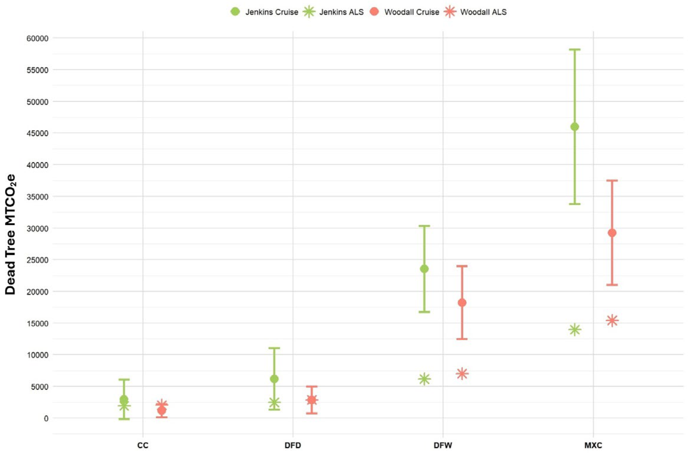
Significant differences were also observed between the biomass equations in terms of dead wood carbon (Figure 5). For every stratum, as well as at the project level, the Jenkins ALS dead wood estimates were lower than the Woodall ALS values; however, the Jenkins cruised dead tree estimates were consistently higher than the Woodall values, similarly to the pattern seen for live tree carbon. The largest percent difference in dead wood estimates between the two equations occurred in the CC stratum for the traditional cruise, where the Jenkins estimate of 2950 MTCO₂e was 2.6 times greater than the Woodall value of 1135 MTCO₂e. In absolute terms, the largest difference in dead wood carbon was approximately 16,756 MTCO₂e and was observed for the MXC stratum of the traditional cruise.

When comparing the ALS estimates to the traditional cruise estimates at the project level, the observed percent difference was 17.0% with the Jenkins biomass equation and 13.1% with the Woodall equation. Additionally, the percent differences between the Jenkins- and Woodall-derived estimates for each quantification approach (ALS and traditional cruise) were 12.8% and 16.7%, respectively.

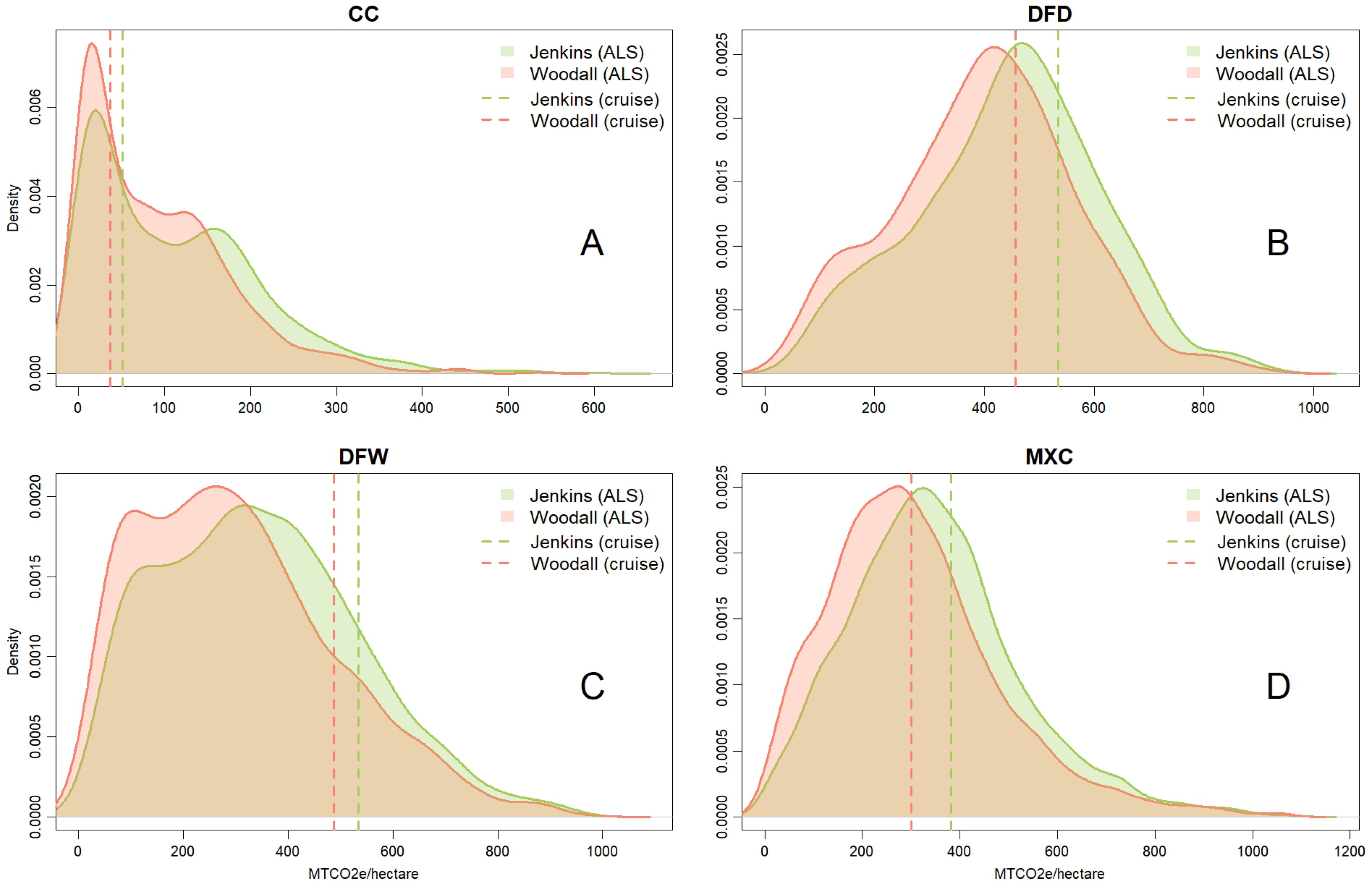
Density distributions of ALS-estimated MTCO₂e per hectare revealed substantial within-stratum variability across all strata (Figure 6). Although all distributions were right-skewed, those for the DFD and MXC strata more closely approximated normality compared to the other strata. Estimates derived using the Jenkins and Woodall biomass equations were strongly correlated, with Jenkins consistently producing higher MTCO₂e values than Woodall, mirroring the patterns reported in Table 3 and Table 4. The CC stratum exhibited a pronounced bimodal distribution, with one mode at approximately 15–19 MTCO₂e per hectare and a second, higher mode at approximately 120 MTCO₂e per hectare for Woodall estimates and 160 MTCO₂e per hectare for Jenkins estimates. In contrast, for the DFW stratum, the cruise-based mean estimates were noticeably higher than the majority of ALS-derived estimates. For the DFD and MXC strata, the cruise means aligned closely with the dominant modes of the ALS-derived distributions, irrespective of the biomass equation applied.

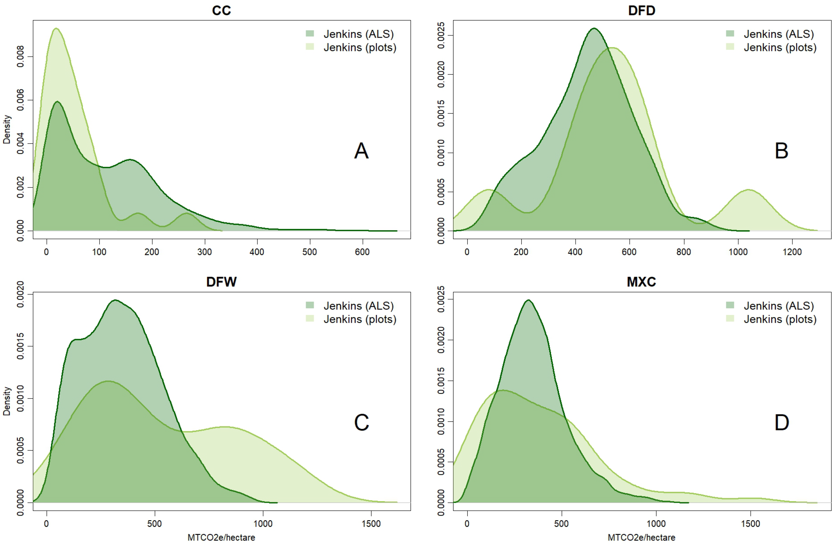
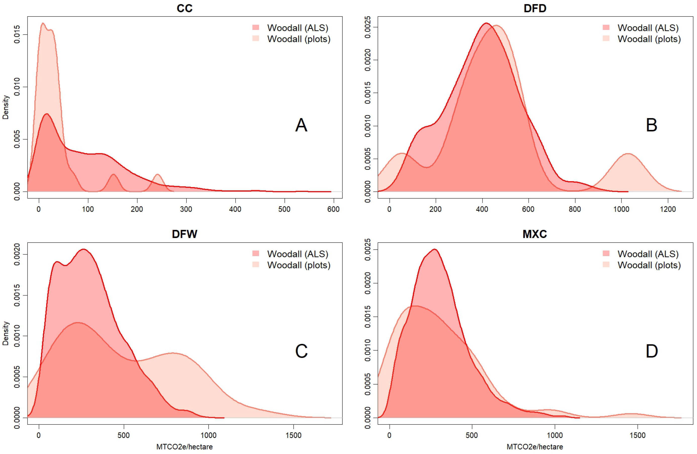
Comparisons between density distributions of MTCO₂e per hectare derived from field-measured plots and those estimated from ALS indicated greater volatility in the field-based distributions, which frequently exhibited two or three distinct modes (Figure 7 and Figure 8). As observed previously, estimates derived from the Jenkins and Woodall biomass equations were strongly correlated and displayed similar stratum-specific patterns. For most strata, with the exception of CC, the range of MTCO₂e per hectare was larger for field plots than for ALS-derived estimates, indicating that some field plots contained higher levels of stored carbon than those detected by the ALS-based inventory.

3.2. SOC Results

Four soil samples were removed as outliers, leaving 128 soil cores across the four strata. Strata level soil organic carbon results for the 0–30 cm depth layer are shown in

Table 5. Per strata estimates of the 0–30 cm soil organic carbon stock densities.

Strata	Mean (Mg/ha)	Margin of Error at 90% Confidence	Site Count
CC	61.5	5.7	25
DFD	56.4	12.2	9
DFW	66.8	7.5	30
MXC	67.3	5.7	64

. At the project level, results were 29.1 +/− 1.6 tons/acre or 65.3 +/− 3.6 Mg/ha for the 0–30 cm layer. For the 0–100 cm layer, the project level mean was 10.8 +/− 1.3 tons/acre or 24.2 +/− 3.0 MG/ha.

3.3. Carbon Dating Results

Results from the carbon dating of two meter cores is shown in

Table 6. Conventional age and calendar calibration by depth layer for meter cores at sites 1 and 2.

Site	Depth Layer (cm)	Conventional Age	Calendar Calibration
1	0–15	102.27 +/− 0.38 pMC	(83.3%) 2013–2018 cal AD; (12.2%) 1955–1956 cal AD
1	15–30	490 +/− 30 BP	(95.4%) 1404–1452 cal AD
1	30–60	1820 +/− 30 BP	(69.3%) 152–256 cal AD; (22.2%) 284–326 cal AD; (4%) 130–144 cal AD
1	60–100	5360 +/− 30 BP	(28.2%) 4136–4054 cal BC; (24.5%) 4268–4216 cal BC; (24.1%) 4206–4159 cal BC; (18.6%) 4328–4286 cal BC
2	0–15	102.78 +/− 0.38 pMC	(81.7%) 2012–2016 cal AD; (13.7%) 1955–1956 cal AD
2	15–30	100.50 +/− 0.38 pMC	(48.7%) 1954–1955 cal AD; (45.9%) 2018–2019 cal AD
2	30–60	660 +/− 30 BP	(48.4%) 1278–1325 cal AD; (47%) 1352–1394 cal AD
2	60–100	3640 +/− 30 BP	(76.4%) 2059–1919 cal BC; (18%) 2135–2082 cal BC

. The carbon dating was performed by the Beta Analytics lab [53]. The results are provided in the two columns: the “Conventional Age” is the conventional radiocarbon age and the “Calendar Calibration” is the result of applying the “High-Probability Density Range Method” or HPD [54] for conversion to calendar year equivalents, with the likelihood in parentheses. The analysis of recent material is challenging due to atomic bomb testing and the prevalence of carbon formed post-1950. This newer carbon is measured in “percent modern carbon” (pMC) units. Carbon dating site 1 is located at (46.84123, −116.78015) and site 2 is located at (46.78402, −116.79714).

The depth variation age of the two cores is somewhat similar, with the exception of the 15–30 cm layer. It appears that this layer at site 1 is older (pre 1950) material, whereas the material in this depth at site 2 is modern. It is possible this is a result of differences in soil disturbance and other management differences at the two sites. Both sites were harvested around 2000; however, site 1 was reforested and is currently treed, whereas site 2 has remained in a cleared state.

Carbon stock density measurements showed that, on average, the 0–30 cm layer contains approximately 30 tons/acre soil organic carbon and the 30–100 cm layer of approximately 10 tons/acre. The differences in the 0–30 cm layer noted above indicate the need for better understanding of the above-ground site history and its impact on the formation of below-ground carbon. However, on average, most of the soil carbon appears to have formed within the last ~70 years. With this rough assumption, we estimate a nominal rate of soil carbon accumulation of 0.4 tons/acre/year for the 0–30 cm layer.

4. Discussion

In this study, we demonstrated that ALS-derived carbon quantifications can be successfully executed, provided that the appropriate data inputs and processing capabilities are in place. This is significant, as many landowners and project proponents already have access to ALS data for their forested lands, which could be leveraged for carbon crediting projects. With the growing trend of utilizing ALS for standard forest inventories and the recent allowance of LiDAR-derived parameters in some carbon registry methodologies [40,55], it was logical to evaluate its capabilities for carbon inventories. ALS technology offers a high level of precision and efficiency in capturing the forest structure, making it an ideal tool for large-scale carbon assessments. This is emphasized for projects in remote areas with access limitations. By validating its potential for carbon quantification, this research helps to unlock new opportunities for landowners to participate in carbon credit markets and supports the broader transition toward more advanced, scalable methods in forest inventory and management. However, along with opportunities come new challenges. The most prominent challenge currently facing the integration of near-census ALS-workflows in modern forest management carbon crediting projects is the requirement of traditional, plot-based sampling for forest carbon quantification. The current approved IFM and ARR methodologies require periodic monitoring of permanent sample plots within the project area, combined with verification of calculated carbon sequestration through a certified third-party verification and validation body (VVB). Because ALS methods like ForestView^® create wall-to-wall robust samples derived using complex algorithms and workflows, the measurement schematic is closer to a complete census than a traditional sample-based inventory. Currently, census inventories are not included as options for IFM methodologies [38,49] and are only allowed for forests that are smaller than 1 hectare in size for the VCS ARR methodology VM0047 [40]. Near-census level inventory alternatives, such as those derived from ALS, are largely unexplored in their applicability to carbon credit markets and will require future research.

In addition to its applicability for inventories of mature forests, like those common within our study area that would likely fall within the scope of IFM projects or theoretical late-stage ARR projects, ALS has been found to be effective for inventories of young trees, especially when grown in open, plantation-like environments [56]. The applicability of ALS inventories across both mature and early-stage forests indicates a potential for the incorporation of ALS data across all stages of IFM and ARR CDR projects, though more research is required.

Rather than determining which sampling method was more accurate, this study aimed to assess the similarities and differences in carbon estimates between ALS-derived and traditional carbon quantifications. Comparing ALS estimates to the 80% confidence intervals around the traditional sampling estimates, similar to the approach taken by Kondratev et al., 2025, proved to be a straightforward way to determine equivalence for this particular application [52]. This approach may provide a valuable framework for future research aimed at comparing sample-based methods with more robust, near-population datasets, offering insights into where the methods align and where discrepancies exist. We acknowledge the fact that the uncertainty in ALS estimates was not computed and used in this analysis. To date, challenges to quantifying the overall error associated with census-like estimates which are the product of large and highly complex modeling chains like ForestView^® exist. The ability to quantify such error would likely allow for additional statistical testing, providing further clarity on how these methods compare.

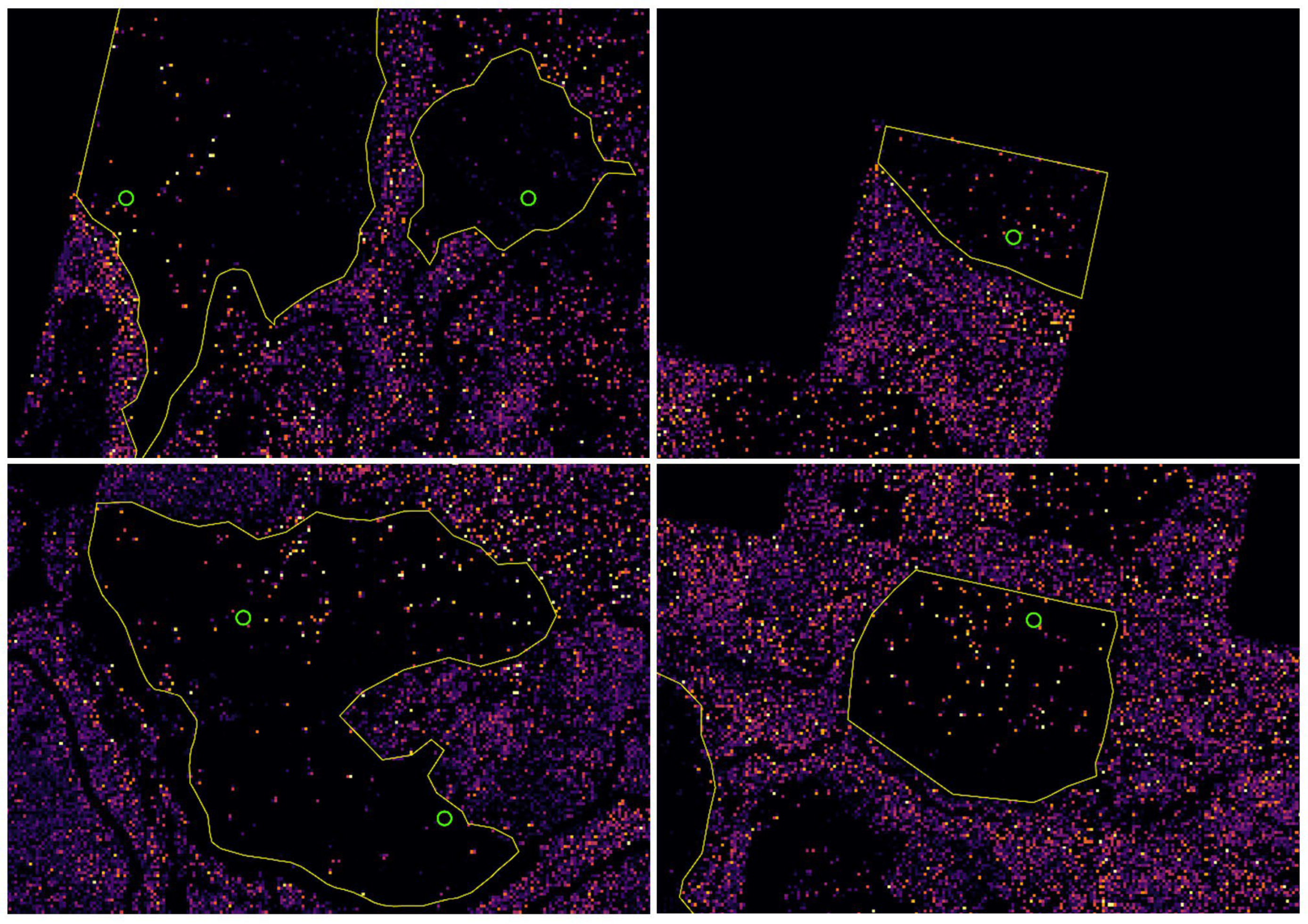
Regardless of the biomass equation used, we found the percent difference between the ALS and traditional quantification to be less than or equal to 17% at the project level. Our findings showed that some ALS and traditional cruise estimates were similar at the carbon pool and strata levels, while others differed. For example, in the CC stratum, ALS detected pockets of residual trees that were missed in the traditional inventory due to the random nature of plot placement, leading to higher ALS values (Figure 9).

In light of this, traditional carbon inventories with lower sampling intensities can run the risk of misrepresenting the true variance in carbon stocks. In addition to the CC stratum, the multimodal density distributions of plot-level MTCO₂e per hectare in the DFD stratum also indicate high variation and volatility resulting from the small sample size of only nine plots (Figure 7 and Figure 8). For certain project types—such as facilitated regeneration, in which a uniform grid-based planting system is not the starting condition—this could be an important distinction. This sampling bias should be a crucial consideration any time a traditional sample-based inventory is applied to a highly heterogeneous landscape, especially if only a subset of plots, or even newly established plots, will be used for project verification purposes. ALS inventories that capture a more accurate representation of true forest conditions in such scenarios are likely more adverse to sampling error.

Differences in dead tree carbon estimates were also common across methods. ALS generally underestimated dead tree carbon relative to the sample-based inventory for all strata. The only exceptions occurred in the CC and DFD strata, where ALS estimates were higher than the traditional inventory when using the Woodall equations. Estimates derived from the Woodall equations align more closely with expectations, as more dead wood should be visible to ALS in more open conditions, such as recently harvested areas or lower-density stands (CC and DFD strata). Conversely, the under-prediction of dead wood in the DFW and MXC strata is consistent with known ALS limitations; subcanopy trees—including suppressed, dying, and dead trees—can be difficult to detect with ALS, especially when using top-down watershed or local maxima algorithms like those within ForestView^®. While effective at delineating dominant and codominant stems, especially those with conical or pyramidal crown architectures, these algorithms are inherently constrained in their ability to detect understory trees beneath overstory canopies. Therefore, lower estimates relative to the sample-based inventory are unsurprising. From this perspective, traditional field-based inventories may currently have an advantage, given the existing technologies. For ALS-based approaches, applying an adjustment factor or bias correction could help address the likely underestimation of dead tree carbon. These findings and limitations should be carefully considered when estimates of dead tree carbon are required.

Although not always significant, a similar pattern of underestimation was observed for live tree carbon in DFD, DFW, and MXC strata. Other studies have proven the accuracy of ALS to identify trees that contribute a large majority of the wood volume [20,21], and therefore carbon, so it is logical to consider the possibility of a significant overestimation of live tree carbon in the DFW strata on behalf of the traditional inventory when considering the random placement of 32 plots across 1730 acres again. Despite these differences, we found that the live tree carbon and total carbon estimates were statistically similar for the MXC strata, which accounted for half of the study area and contributed a majority of the tree carbon. This suggests that while carbon estimates may be slightly different when using an ALS inventory compared to a traditional one, the overall differences are not substantial enough to discount ALS as a viable method for carbon assessment. Given that carbon credit generation depends on tracking carbon flux throughout a project’s lifetime, the ability of a method to consistently quantify carbon and realistically capture stock changes—such as those from growth, harvest, and other dynamics—may be more important than ensuring that new workflows produce results that are equivalent to historic ones. The highly repeatable and wall-to-wall nature of ALS workflows may therefore be particularly advantageous from this perspective.

The selection of a biomass equation is largely governed by the specific carbon crediting protocol of interest. The equations analyzed in this study are widely used for biomass estimation and are fairly common in many modern carbon credit registry protocols [5,38,40]. A key takeaway from the study results is the significant difference in the estimates derived from the Jenkins and Woodall equations. At the project level, the percent differences between ALS and the traditional cruise were 17.0% and 13.1%, respectively, when applying the Jenkins and Woodall biomass equations. Notably, the Woodall methodology involves the calculation of the stem volume, which requires the additional input of tree height compared to the single input of DBH in the Jenkins equation; this likely contributed to the observed differences in the final values. This could be crucial if or when an opportunity exists to re-establish project baselines by replacing traditional sampling methods with ALS-based quantification approaches. Although the discrepancies between ALS and traditional estimates were smaller with the Woodall equations, the estimates remained consistently lower than those produced by Jenkins. Within each quantification methodology (ALS and traditional cruise), the Woodall estimates were 12.8% and 16.7% lower than the Jenkins estimates, respectively. These findings highlight the generalizations that are inherent in commonly used biomass equations and reinforce the concerns raised by Haya et al. regarding the reliability of some current biomass estimation methods. The choice between these equations significantly impacts the final estimates, but the effect may be less pronounced when focusing on carbon flux—i.e., the difference in estimated carbon stocks between multiple quantifications. Future research aimed at understanding the broader implications of biomass equation selection would be a valuable contribution to the field.

While this study primarily focused on comparing tree carbon quantified using traditional and ALS sampling methods, the inclusion of SOC and carbon dating data provided valuable insights into the durability of forest carbon pools extending beyond tree carbon stocks. Many current IFM protocols consider the SOC flux to be minimal, and as a result, this carbon pool is often excluded from these types of projects, with some exceptions. However, other project types, such as ARR, allow for SOC quantification [6,36,40]. Given our ability to collect this data, we sought to explore the potential contribution of SOC to the total carbon stocks. The SOC estimates presented in this study were significant in relation to the overall carbon stored within the project area, but they provide limited insight into potential changes in SOC over time, particularly in the context of baseline and project scenarios.

5. Conclusions

This study compared a modern ALS-based inventory approach to a traditional field-based method to assess differences in carbon quantification estimates, the magnitude of those differences, and whether the choice of biomass equation (Jenkins versus Woodall) meaningfully influenced the total quantification estimates. While ALS and traditional methodologies were consistent for the largest and most carbon-rich stratum (MXC), regardless of the applied biomass equation, differences were observed in carbon pools and other strata that inform the considerations users may have for each approach. ALS can underestimate biomass in closed canopy stands with many suppressed or intermediate trees or where substantial standing tree mortality is present. However, ALS demonstrated comparable or superior performance relative to traditional methods across multiple forest conditions, capturing a greater degree of landscape heterogeneity. Traditional inventories can reliably account for sub-canopy suppressed and intermediate trees at the plot level; however, these methods depend on scaling data to non-sampled areas, potentially introducing significant uncertainty and variance when extrapolated across large areas.

Overall, the results of this study suggest that ALS workflows can produce carbon pool estimates that are comparable to those of traditional inventories, as shown by the MXC stratum and several others. This study further shows that variance in carbon pool estimates can exist when different methods are applied and when various forested conditions are present—especially more open, less dense forests—where ALS-based methods offer some clear advantages. These findings suggest that ALS-based methods can add value to large-scale carbon quantification calculations across extensive landscapes and have the potential to play a significant role in the future of carbon crediting systems. This does not discount the limitations of ALS in dense forest conditions, and perhaps a hybrid approach that incorporates traditional sampling with ALS collections may be preferable for some forested landscapes. Additionally, the carbon registry methodologies and implications of third-party verification remain key hurdles for broader ALS adoption in carbon crediting protocols.

The inclusion of the soil organic carbon (SOC) pool in this study provided a more comprehensive understanding of the total carbon present and its durability, which is essential for some project types. Combining advanced remote sensing and SOC pools with established forest management protocols offers the opportunity to refine and strengthen the framework available to carbon credit projects, ensuring they are scalable, accurate, and aligned with evolving industry standards.

Beyond current applications, ALS is likely to offer immediate benefits to the practices of forest certification, corporate greenhouse gas accounting, and the validation of standing carbon stocks, which can aid in forest management and land acquisition decisions. Looking ahead, additional research efforts should focus on ALS-derived uncertainty in LiDAR-based carbon calculations, on emerging remote sensing technologies, and on the refinement of biomass equations, all of which may lead to improvements in the accuracy and precision of carbon quantification efforts.

References

1. Sandalow, D.; Aines, R.; Friedmann, J.; Mccormick, C.; Sanchez, D. Biomass Carbon Removal and Storage (BiRCS) Roadmap; LLNL-TR-815200; LLNL: Livermore, CA, USA, 2020. [Google Scholar]
2. van der Gaast, W.; Sikkema, R.; Vohrer, M. The contribution of forest carbon credit projects to addressing the climate change challenge. Clim. Policy 2018, 18, 42–48. [Google Scholar] [CrossRef]
3. Haya, B.K.; Evans, S.; Brown, L.; Bukoski, J.; Butsic, V.; Cabiyo, B.; Jacobson, R.; Kerr, A.; Potts, M.; Sanchez, D.L. Comprehensive Review of Carbon Quantification by Improved Forest Management Offset Protocols. Front. For. Glob. Chang. 2023, 6, 958879. [Google Scholar] [CrossRef]
4. ACR. The ACR Standard: Requirements and Specifications for the Quantification, Monitoring, Reporting, Verification, and Registration of Project-Based GHG Emissions Reductions and Removals; Version 8.0 ed.; Winrock International: Arlington, VA, USA, 2023. [Google Scholar]
5. ARB. Compliance Offset Protocol US Forest Projects; California Environmental Protection Agency: Sacramento, CA, USA, 2015. [Google Scholar]
6. Gold Standard. Methodology for Afforestation/Reforestation (A/R) GHGs Emission Reduction & Sequestration; Version 2.1 ed.; The Gold Standard Foundation: Geneva, Switzerland, 2024. [Google Scholar]
7. VCS. VCS Standard, v4.7; Version 4.7 ed.; Verra: Washington, DC, USA, 2024. [Google Scholar]
8. Requena Suarez, D.; Rozendaal, D.M.A.; De Sy, V.; Phillips, O.L.; Alvarez-Dávila, E.; Anderson-Teixeira, K.; Araujo-Murakami, A.; Arroyo, L.; Baker, T.R.; Bongers, F.; et al. Estimating aboveground net biomass change for tropical and subtropical forests: Refinement of IPCC default rates using forest plot data. Glob. Change Biol. 2019, 25, 3609–3624. [Google Scholar] [CrossRef]
9. Oehmcke, S.; Li, L.; Trepekli, K.; Revenga, J.C.; Nord-Larsen, T.; Gieseke, F.; Igel, C. Deep point cloud regression for above-ground forest biomass estimation from airborne LiDAR. Remote Sens. Environ. 2024, 302, 113968. [Google Scholar] [CrossRef]
10. Booth, D.T.; Cox, S.E.; Meikle, T.; Zuuring, H.R. Ground-cover measurements: Assessing correlation among aerial and ground-based methods. Environ. Manag. 2008, 42, 1091–1100. [Google Scholar] [CrossRef] [PubMed]
11. Mäkinen, A.; Kangas, A.; Nurmi, M. Using Cost-Plus-Loss Analysis to Define Optimal Forest Inventory Interval and Forest Inventory Accuracy. Silva Fenn. 2012, 46, 211–226. [Google Scholar] [CrossRef]
12. Cunia, T. Some Theory on Reliability of Volume Estimates in a Forest Inventory Sample. For. Sci. 1965, 11, 115–128. [Google Scholar] [CrossRef]
13. Hetzer, J.; Huth, A.; Wiegand, T.; Dobner, H.J.; Fischer, R. An Analysis of Forest Biomass Sampling Strategies Across Scales. Biogeosciences 2020, 17, 1673–1683. [Google Scholar] [CrossRef]
14. Scott, C.T. Sampling methods for estimating change in forest resources. Ecol. Appl. 1998, 8, 228–233. [Google Scholar] [CrossRef]
15. Berger, A.; Gschwantner, T.; McRoberts, R.E.; Schadauer, K. Effects of measurement errors on individual tree stem volume estimates for the Austrian national forest inventory. For. Sci. 2014, 60, 14–24. [Google Scholar] [CrossRef]
16. Barr, A.G.; Morgenstern, K.; Black, T.A.; McCaughey, J.H.; Nesic, Z. Surface energy balance closure by the eddy-covariance method above three boreal forest stands and implications for the measurement of the CO2 flux. Agric. For. Meteorol. 2006, 140, 322–337. [Google Scholar] [CrossRef]
17. Kurz, W.A.; Hayne, S.; Fellows, M.; Macdonald, J.D.; Metsaranta, J.M.; Hafer, M.; Blain, D. Quantifying the impacts of human activities on reported greenhouse gas emissions and removals in Canada’s managed forest: Conceptual framework and implementation. Can. J. For. Res. 2018, 48, 1227–1240. [Google Scholar] [CrossRef]
18. Kurz, W.A.; Dymond, C.C.; White, T.M.; Stinson, G.; Shaw, C.H.; Rampley, G.J.; Smyth, C.; Simpson, B.N.; Neilson, E.T.; Trofymow, J.A.; et al. CBM-CFS3: A model of carbon-dynamics in forestry and land-use change implementing IPCC standards. Ecol. Model. 2009, 220, 480–504. [Google Scholar] [CrossRef]
19. Zhao, B.; Zhuang, Q.; Shurpali, N.; Köster, K.; Berninger, F.; Pumpanen, J. North American boreal forests are a large carbon source due to wildfires from 1986 to 2016. Sci. Rep. 2021, 11, 7723. [Google Scholar] [CrossRef] [PubMed]
20. Corrao, M.V.; Sparks, A.M.; Smith, A.M.S. A Conventional Cruise and Felled-Tree Validation of Individual Tree Diameter, Height and Volume Derived from Airborne Laser Scanning Data of a Loblolly Pine (P. taeda) Stand in Eastern Texas. Remote Sens. 2022, 14, 2567. [Google Scholar] [CrossRef]
21. Sparks, A.M.; Corrao, M.V.; Keefe, R.F.; Armstrong, R.; Smith, A.M.S. An Accuracy Assessment of Field and Airborne Laser Scanning-Derived Individual Tree Inventories using Felled Tree Measurements and Log Scaling Data in a Mixed Conifer Forest. For. Sci. 2024, 70, 228–241. [Google Scholar] [CrossRef]
22. Sparks, A.M.; Smith, A.M.S. Accuracy of a lidar-based individual tree detection and attribute measurement algorithm developed to inform forest products supply chain and resource management. Forests 2022, 13, 3. [Google Scholar] [CrossRef]
23. Lefsky, M.A.; Cohen, W.B.; Parker, G.G.; Harding, D.J. LiDAR Remote Sensing for Ecosystem Studies. Bioscience 2002, 52, 19–30. [Google Scholar] [CrossRef]
24. White, J.C.; Coops, N.C.; Wulder, M.A.; Vastaranta, M.; Hilker, T.; Tompalski, P. Remote Sensing Technologies for Enhancing Forest Inventories: A Review. Can. J. Remote Sens. 2016, 42, 619–641. [Google Scholar] [CrossRef]
25. Xu, D.; Wang, H.; Xu, W.; Luan, Z.; Xu, X. LiDAR applications to estimate forest biomass at individual tree scale: Opportunities, challenges and future perspectives. Forests 2021, 12, 550. [Google Scholar] [CrossRef]
26. Lamlom, S.H.; Savidge, R.A. A reassessment of carbon content in wood: Variation within and between 41 North American species. Biomass Bioenergy 2003, 25, 381–388. [Google Scholar] [CrossRef]
27. Thomas, S.C.; Martin, A.R. Carbon content of tree tissues: A synthesis. Forests 2012, 3, 332–352. [Google Scholar] [CrossRef]
28. Beland, M.; Parker, G.; Sparrow, B.; Harding, D.; Chasmer, L.; Phinn, S.; Antonarakis, A.; Strahler, A. On promoting the use of lidar systems in forest ecosystem research. For. Ecol. Manag. 2019, 450, 117484. [Google Scholar] [CrossRef]
29. Hummel, S.; Hudak, A.T.; Uebler, E.H.; Falkowski, M.J.; Megown, K.A. A Comparison of Accuracy and Cost of LiDAR versus Stand Exam Data for Landscape Management on the Malheur National Forest. J. For. 2011, 109, 267–273. [Google Scholar] [CrossRef]
30. Reutebuch, S.E.; Andersen, H.E.; Mcgaughey, R.J. Light Detection and Ranging (LIDAR): An Emerging Tool for Multiple Resource Inventory. J. For. 2005, 103, 286–292. [Google Scholar] [CrossRef]
31. Gobakken, T.; Næsset, E.; Nelson, R.; Bollandsås, O.M.; Gregoire, T.G.; Ståhl, G.; Holm, S.; Ørka, H.O.; Astrup, R. Estimating biomass in Hedmark County, Norway using national forest inventory field plots and airborne laser scanning. Remote Sens. Environ. 2012, 123, 443–456. [Google Scholar] [CrossRef]
32. McRoberts, R.E.; Tomppo, E.O. Remote sensing support for national forest inventories. Remote Sens. Environ. 2007, 110, 412–419. [Google Scholar] [CrossRef]
33. Kelly, M.; Di Tommaso, S. Mapping forests with Lidar provides flexible, accurate data with many uses. Calif. Agric. 2015, 69, 14–20. [Google Scholar] [CrossRef]
34. Knott, J.A.; Liknes, G.C.; Giebink, C.L.; Oh, S.; Domke, G.M.; McRoberts, R.E.; Quirino, V.F.; Walters, B.F. Effects of outliers on remote sensing-assisted forest biomass estimation: A case study from the United States national forest inventory. Methods Ecol. Evol. 2023, 14, 1587–1602. [Google Scholar] [CrossRef]
35. Salvini, R.; Mastrorocco, G.; Esposito, G.; Di Bartolo, S.; Coggan, J.; Vanneschi, C. Use of a remotely piloted aircraft system for hazard assessment in a rocky mining area (Lucca, Italy). Nat. Hazards Earth Syst. Sci. 2018, 18, 287–302. [Google Scholar] [CrossRef]
36. ACR. Methodology for the Quantification, Monitoring, Reporting and Verification of Greenhouse Gas Emission Reductions and Removals from Afforestation & Reforestation of Degraded Land; Version 1.2 ed.; Winrock International: Arlington, VA, USA, 2017. [Google Scholar]
37. Gold Standard. Gold Standard for the Global Goals Land-Use & Forests Activity Requirements; Version 1.0 ed.; The Gold Standard Foundation: Geneva, Switzerland, 2017. [Google Scholar]
38. ACR. Methodology for the Quantification, Monitoring, Reporting and Verification of Greenhouse Gas Emission Reductions and Removals from Improved Forest Management on Non-Federal U.S. Forestland; Version 2.1 ed.; Winrock International: Arlington, VA, USA, 2024. [Google Scholar]
39. Gold Standard. Gold Standard for the Global Goals Land Use & Forests Activity Requirements; Version 1.2.1 ed.; The Gold Standard Foundation: Geneva, Switzerland, 2020. [Google Scholar]
40. VCS. VCS Methodology VM0047: Afforestation, Reforestation and Revegetation; Version 1.0 ed.; Verra: Washington, DC, USA, 2023. [Google Scholar]
41. Pearson, T.; Walker, S.; Brown, S. Sourcebook for Land Use, Land-Use Change and Forestry Projects; BioCarbon Fund at Winrock International: Arlington, VA, USA, 2005. [Google Scholar]
42. Riegl USA. Riegl 1560ii LiDAR Sensor. 2022. Available online: http://www.riegl.com/nc/products/airborne-scanning/produktdetail/product/scanner/68/ (accessed on 17 October 2025).
43. SOMAG Jena Germany. Gyro Stabilization Mount (GSM) 4000 [WWW Document]. 2022. Available online: https://www.somag-ag.de/products/airborne-gyro-mounts/gsm-4000/ (accessed on 15 October 2025).
44. Riegl USA. RiPROCESS [WWW Document]. 2022. Available online: http://www.rieglusa.com/index.html (accessed on 17 October 2025).
45. Silva, C.A.; Hudak, A.T.; Vierling, L.A.; Loudermilk, E.L.; O’Brien, J.J.; Hiers, J.K.; Jack, S.B.; Gonzalez-Benecke, C.; Lee, H.; Falkowski, M.J.; et al. Imputation of Individual Longleaf Pine (Pinus palustris Mill.) Tree Attributes from Field and LiDAR Data. Can. J. Remote Sens. 2016, 42, 554–573. [Google Scholar] [CrossRef]
46. Yu, X.; Hyyppä, J.; Litkey, P.; Kaartinen, H.; Vastaranta, M.; Holopainen, M. Single-sensor solution to tree species classification using multispectral airborne laser scanning. Remote Sens. 2017, 9, 108. [Google Scholar] [CrossRef]
47. Jenkins, J.C.; Chojnacky, D.C.; Heath, L.S.; Birdsey, R.A. National-Scale Biomass Estimators for United States Tree Species. For. Sci. 2003, 49, 12–35. [Google Scholar] [CrossRef]
48. Woodall, C.W.; Heath, L.S.; Domke, G.M.; Nichols, M.C. Methods and Equations for Estimating Aboveground Volume, Biomass, and Carbon for Trees in the U.S. Forest Inventory, 2010; Gen. Tech. Rep. NRS-88; US Department of Agriculture, Forest Service, Northern Research Station: Newtown Square, PA, USA, 2011; Volume 88, pp. 1–30. [Google Scholar] [CrossRef]
49. VCS. VCS Methodology VM0045: Improved Forest Management Using Dynamic Matched Baselines from National Forest Inventories; Version 1.1 ed.; Verra: Washington, DC, USA, 2024. [Google Scholar]
50. Raile, G.K. Estimating Stump Volume; Res. Pap. NC-224; US Department of Agriculture, Forest Service, North Central Forest Experiment Station: St. Paul, MN, USA, 1982; Volume 224, pp. 1–4. [Google Scholar] [CrossRef]
51. Heath, L.S.; Hansen, M.H.; Smith, J.E.; Smith, W.B.; Miles, P.D. Investigation into calculating tree biomass and carbon in the FIADB using a biomass expansion factor approach. In Proc. RMRS-P-56CD, Proceedings of the 2008 Forest Inventory and Analysis (FIA) Symposium, Park City, UT, USA, 21–23 October 2008; U.S. Department of Agriculture, Forest Service, Rocky Mountain Research Station: Fort Collins, CO, USA, 2009; Volume 56, pp. 1–26. [Google Scholar]
52. Kondratev, M.; Corrao, M.V.; Armstrong, R.; Smith, A.M. Assessing the Uncertainty of Traditional Sample-Based Forest Inventories in Mixed and Single Species Conifer Systems Using a Digital Forest Twin. Forests 2025, 16, 1617. [Google Scholar] [CrossRef]
53. Beta Analytic. Calibration of Carbon 14 Dating Results [WWW Document]. 2022. Available online: https://www.radiocarbon.com/calendar-calibration-carbon-dating.htm (accessed on 5 February 2025).
54. Ramsey, C.B. Bayesian analysis of radiocarbon dates. Radiocarbon 2009, 51, 337–360. [Google Scholar] [CrossRef]
55. VCS. VCS Methodology VM0015: Avoided Unplanned Deforestation; Version 1.2 ed.; Verra: Washington, DC, USA, 2023. [Google Scholar]
56. Watt, M.S.; Meredith, A.; Watt, P.; Gunn, A. Use of LiDAR to estimate stand characteristics for thinning operations in young Douglas-fir plantations. N. Z. J. For. Sci. 2013, 43, 18. [Google Scholar]
57. Jenkins, J.C.; Chojnacky, D.C.; Heath, L.S.; Birdsey, R.A. Comprehensive Database of Diameter-Based Biomass Regressions for North American Tree Species; Gen. Tech. Rep. NE-319; US Department of Agriculture, Forest Service, Northern Research Station: Newtown Square, PA, USA, 2004; pp. 1–45. [Google Scholar]
Figure 1. ALS-derived 95th percentile tree height across the UIEF, located in the Palouse Range of northern Idaho as indicated by the star symbol.
Remotesensing 18 00547 g001
Figure 2. ALS flight lines in proximity to forest and soil sampling locations within the UIEF study area.
Remotesensing 18 00547 g002
Figure 3. LiDAR returns for a heavily forested subset of the UIEF study area.
Remotesensing 18 00547 g003
Figure 4. Jenkins and Woodall ALS estimates in relation to field cruise means and 80 percent confidence intervals for CC (A), DFD (B), DFW (C), and MXC (D) strata.
Remotesensing 18 00547 g004
Figure 5. Cruised and ALS-derived dead tree carbon estimates for Jenkins and Woodall biomass approaches.
Remotesensing 18 00547 g005
Figure 6. Density distributions of ALS-derived MTCO2e estimates for both Jenkins and Woodall approaches across the entire study area in relation to field cruise means for CC (A), DFD (B), DFW (C), and MXC (D) strata.
Remotesensing 18 00547 g006
Figure 7. Density distributions of field plot estimates of MTCO2e per hectare, relative to the ALS estimates for CC (A), DFD (B), DFW (C), and MXC (D) strata, using the Jenkins biomass equations.
Remotesensing 18 00547 g007
Figure 8. Density distributions of field plot estimates of MTCO2e per hectare, relative to the ALS estimates for CC (A), DFD (B), DFW (C), and MXC (D), strata using the Woodall biomass equations.
Remotesensing 18 00547 g008
Figure 9. Field measured plot locations (green circles) in proximity to ALS-estimated MTCO2e within portions of the CC stratum (yellow polygons). Darker pixels indicate lower MTCO2e per hectare, whereas lighter colors represent higher MTCO2e per hectare.
Remotesensing 18 00547 g009