Article

AI-Driven Wetland Mapping Across Diverse Natural Regions of Alberta, Canada, Using Combined Airborne and Satellite Remote Sensing Data

1
Alberta Biodiversity Monitoring Institute, University of Alberta, Edmonton, AB T6G 2E9, Canada
2
Ducks Unlimited Canada, Edmonton, AB T5P 4W2, Canada
3
Government of Alberta, Environment and Protected Areas, Edmonton, AB T5K 2M4, Canada
*
Author to whom correspondence should be addressed.
Remote Sens. 2026, 18(3), 507; https://doi.org/10.3390/rs18030507
Submission received: 21 November 2025 / Revised: 23 January 2026 / Accepted: 29 January 2026 / Published: 4 February 2026
(This article belongs to the Special Issue Application of Remote Sensing Technology in Wetland Ecology)

Highlights

What are the main findings?
  • AI models integrating multi-sensor satellite data and LiDAR met or exceeded Alberta’s provincial wetland mapping standards across four pilot regions.
  • Deep learning achieved the highest overall accuracies, while machine learning captured finer details and more effectively detected rare wetland types.
What are the implications of the main findings?
  • AI-driven approaches offer a scalable and efficient pathway to modernize wetland inventory mapping and support operational updates across Alberta.
  • Future provincial mapping initiatives should carefully consider the cost–benefit of integrating different technologies, including LiDAR and high-resolution satellite imagery, which offer high impact and scalability but can be costly to acquire.

Abstract
This study evaluates the performance of artificial intelligence (AI) technologies for wetland classification in the province of Alberta, Canada, using integrated remote sensing inputs, including airborne light detection and ranging (LiDAR), orthophotography, and multi-sensor satellite imagery (Sentinel-1, Sentinel-2, PlanetScope). Our primary objective was to assess whether AI-driven modelling approaches, specifically machine learning (ML) and deep learning (DL), can meet Alberta’s provincial wetland mapping standards. We hypothesized that integrating high-resolution LiDAR with multi-seasonal optical and radar data composites into advanced AI algorithms would achieve the required classification accuracy, detail, and minimum mapping unit targets. We tested several methodologies in four ecologically distinct pilot areas representing Alberta’s Boreal, Grassland, and Parkland Natural Regions. AI models included ensemble ML using Extreme Gradient Boosting (XGBoost) and Random Forest, and a DL U-Net convolutional neural network (CNN). AI models were trained on expert-labelled photoplots and validated using in situ field surveys. Our findings demonstrate that both ML and DL models met and, in several cases, exceeded the provincial mapping standards with validation overall accuracies surpassing >70% (form), >80% (class), and >90% (wetland–upland). U-Net CNN models generally produced the highest overall accuracies and most precise wetland extent delineation, but XGBoost offered finer detail and granularity for detailed mapping of rare wetland forms. Integrating LiDAR data and derivatives further enhanced model performance, improving accuracy by as much as 13%. Based on these outcomes, we provide a set of recommendations for scaling up these approaches, focusing on model selection, LiDAR imagery integration, and the continued value of field surveys to support the operational scaling of AI-driven classification approaches for wetland inventory updates across Alberta’s diverse landscapes. However, key challenges remain in scaling up this approach due to the cost of acquiring high-resolution LiDAR and satellite imagery.

Graphical Abstract

1. Introduction

Wetlands are among the most productive ecosystems globally, providing critical ecological services including water quality regulation, flood control, nutrient retention, and essential habitat for wildlife [1]. However, wetlands are experiencing rapid and widespread decline, with an estimated global loss of approximately 3.4 million km2 since 1970, a trend that has been particularly pronounced in Europe and North America [2]. This loss affects a wide range of wetland systems, including swamps, marshes, and open water bodies, which play key hydrological roles and support migratory birds and other wildlife, many of which are species at risk [3]. Key drivers of wetland degradation include land use change, industrial development, and climatic warming, including increasing wildfire frequency and severity [4]. The scale and pace of wetland loss underscore the urgent need for improved monitoring, management, and policy interventions, all of which rely on accurate, spatially explicit, and up-to-date wetland inventories that remain unavailable in many regions [5,6]. In Alberta, Canada, wetlands cover over 28% of the land surface [7], with many designated as Ramsar sites—wetlands designated as important under international environmental treaty [8]. Despite efforts to raise awareness of their benefits [9], the loss of wetlands continues at an alarming rate [10]. For example, it is estimated that 90% of wetland area has been lost in the Prairie Pothole Region of Alberta, primarily due to drainage for agricultural expansion [11]. This loss prompted the development of Alberta’s Wetland Policy [12], which prioritizes avoidance as the primary mitigation strategy when development activities may impact wetlands [13,14]. To meet the needs of this policy, wetland data of high quality and consistency are necessary [15]. Rapidly advancing technologies, such as digital remote sensing (RS), are providing encouraging avenues for meeting these information needs while ensuring adherence to established standards [16]. In Alberta, these standards include strict requirements for wetland classification detail, accuracy, and feature size. Alberta’s wetland mapping standards were established to support the development of a provincial-scale wetland inventory, while considering what was achievable using Earth Observation (EO) data.
Wetlands have traditionally been mapped using a combination of aerial photography, field-based reconnaissance, and manual image interpretation [17]. However, recent advances in low-cost RS data and EO satellite systems have enabled more cost-effective, data-driven, and repeatable wetland mapping at broad scales [18]. Using different regions of the electromagnetic spectrum, RS sensors capture information on water, vegetation, and soil properties, with optical imagery from platforms such as Landsat and Sentinel-2 widely used for wetland mapping and change analysis [19,20,21,22], though performance can be limited in cloud-prone and forested environments such as the boreal biome [23]. In contrast, active synthetic aperture radar (SAR) systems penetrate vegetation, operate independently of solar illumination, and are highly sensitive to wetland dielectric properties [24]. Increasingly, the integration of optical and SAR data has been shown to improve wetland classification performance, particularly in boreal regions [25,26,27], and when complemented by topographic RS data such as light detection and ranging (LiDAR), which provides critical information on elevation, hydrology, and vegetation structure relevant to wetland presence and type [28,29,30,31,32,33].
More recently, wetland mapping has greatly benefited from data science and artificial intelligence (AI)—i.e., machine learning (ML) and deep learning (DL)—technologies [34,35,36,37]. Classic ML algorithms such as Random Forest (RF) and support vector machine (SVM) have been widely applied for wetland classification [38,39,40,41]. More sophisticated AI modelling techniques, such as DL convolutional neural networks (CNNs), have gained traction with usage and novel developments, with varying but encouraging results [42,43]. Prominent examples have demonstrated the value of DL CNNs for wetland classification on both medium-resolution [44,45,46] and high-resolution [47,48,49,50] RS data. The success of DL models, such as CNNs, is owed to their ability to extract hierarchical features (i.e., from simple features in early layers, to more complex and abstract features in deeper layers) from high-dimensional RS imagery for complex landscape classification [51]. Moreover, CNNs are effective at capturing spatial context and landscape patterns, which manifest in wetlands in the form of gradients and transitional zones [52].
The primary aim of this study is to evaluate innovative AI-driven mapping methodologies that have the potential to meet or exceed Alberta’s provincial mapping standards and support repeatable operational inventory development, and updates [16]. Further motivation comes from the limitations of Alberta’s current wetland inventory, the Alberta Merged Wetland Inventory (AMWI; [7]), which is derived from various EO sources, from a range of dates, and completed using different methodologies, resulting in variations in quality and accuracy, and is no longer considered up to date. To our knowledge, this is the first direct evaluation of new RS and data science technologies with regard to the recently adopted provincial standards, which are now central to wetland inventory mapping and updates in Alberta. To achieve this, we piloted state-of-the-art technologies specific to Alberta’s ecological zones, in four areas across the province. More specifically, our goals were to
  • Test AI-based methodologies, including ML and DL, and new EO data including high-resolution airborne LiDAR and photos and commercial and publicly available satellite imagery.
  • Develop wetland inventories for each pilot area and evaluate them against the provincial mapping standards.
  • Provide recommendations on the advantages of new methodologies and their potential for scaling across Alberta to update the provincial wetland inventory.
We expect this study to inform the development of scaled-up, accurate, efficient, and cost-effective wetland mapping and monitoring in Alberta and beyond, to similar landscapes with expansive boreal wetlands, complex parkland areas and, prairie pothole wetland regions.

2. Materials and Methods

2.1. Study Areas

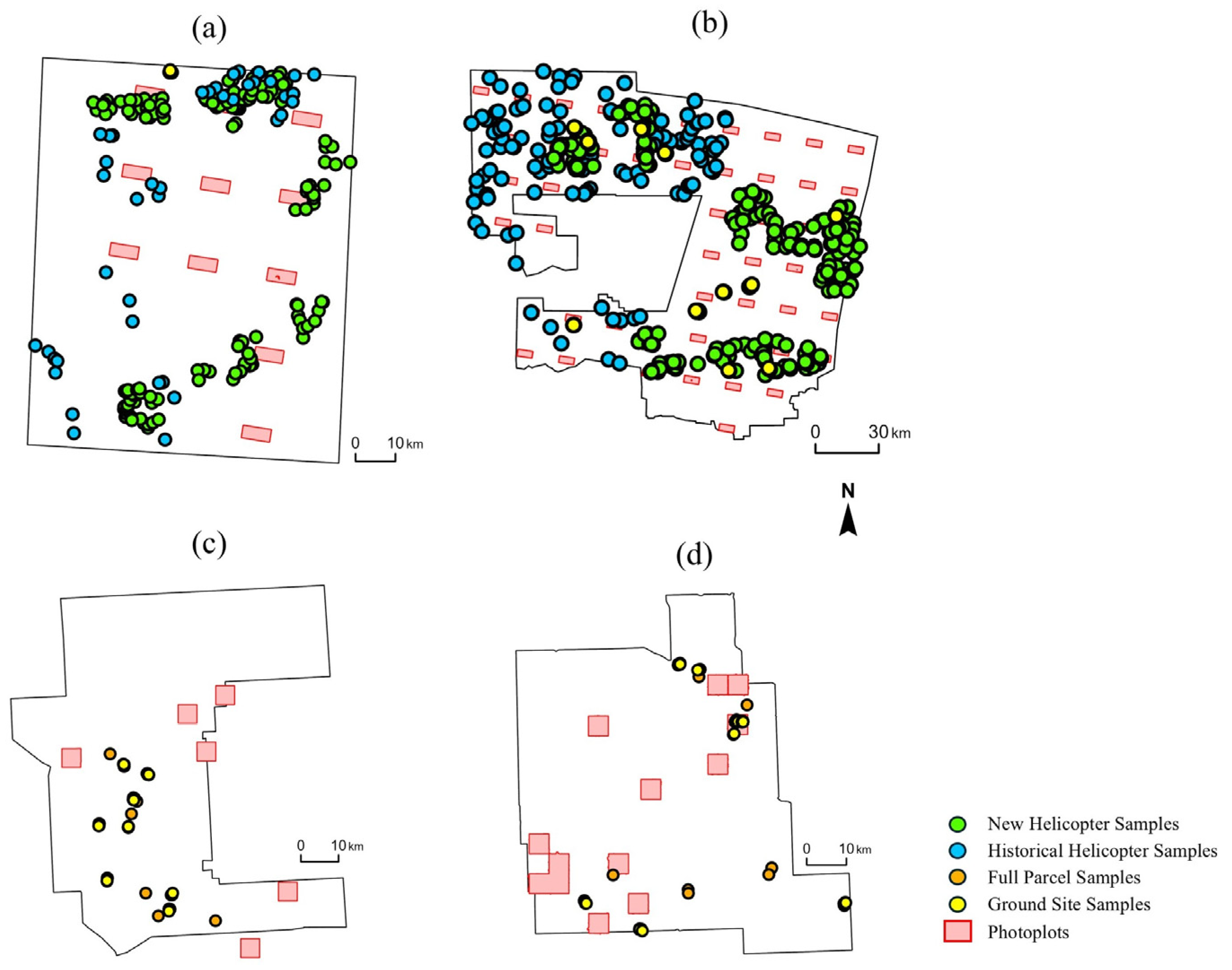
Four pilot areas within the Boreal, Foothills, Parkland, and Grassland Natural Regions were selected for this study to develop effective wetland mapping approaches across Alberta, where a key challenge is to effectively map a wide diversity of wetland types and extent, and that are also situated in a diversity of landscape settings (Figure 1). Alberta’s Natural Regions are characterized by their unique climate, physiographic, vegetation, soil, wildlife, and land use attributes [53]. The four pilot areas were selected within Natural Regions for which the Government of Alberta (GOA) have set wetland mapping standards: Boreal/Foothills and Prairie/Parkland zones. These pilots capture the broad diversity of Alberta’s wetlands, ranging from peatland-dominated systems in the northern forested boreal where wetlands cover large portions of the landscape to the warmer Prairie–Parkland regions in the south where wetlands are smaller, more dynamic, and typically dominated by mineral soil marshes and open water (Table 1). All pilots are supported by extensive validation data and remotely sensed imagery.

2.2. Wetland Definitions and Target Standards

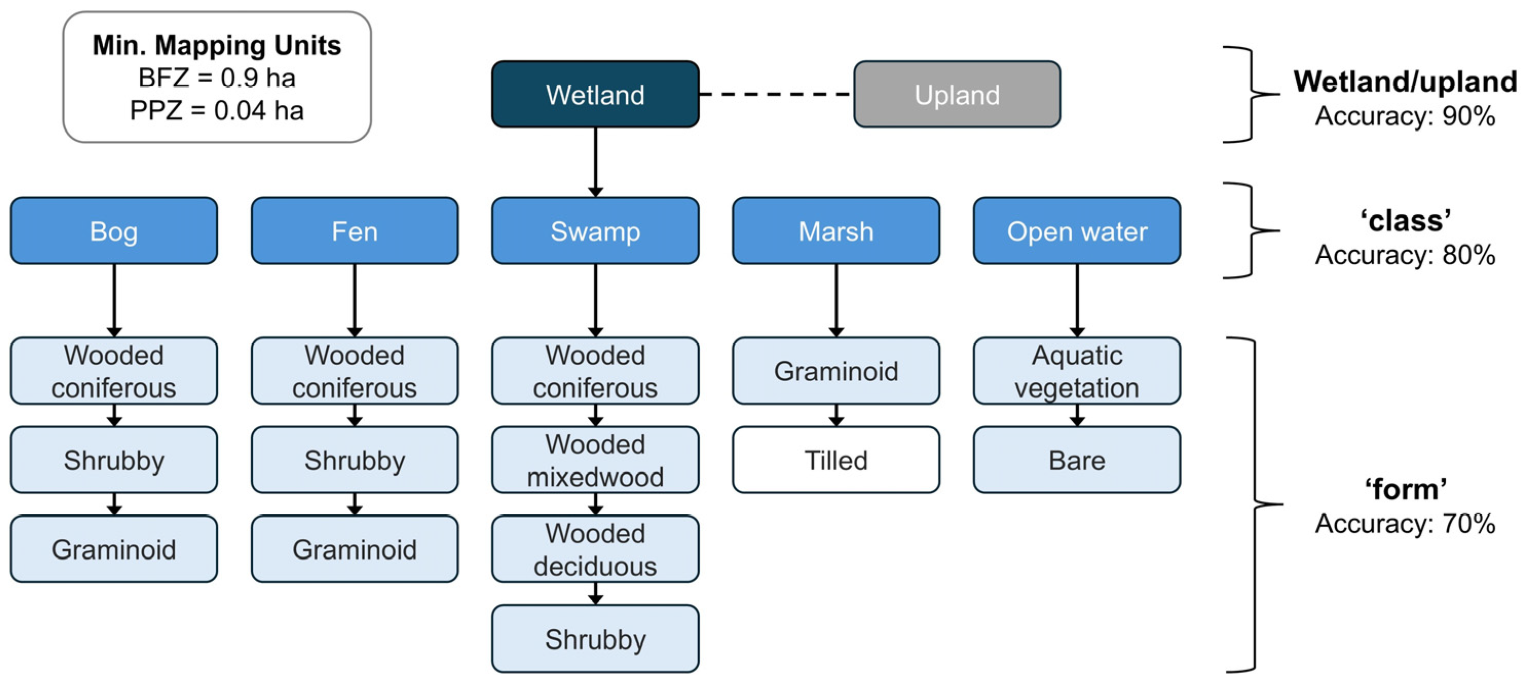
According to the GOA wetland mapping standards [16], and following local nomenclature, thematic classification level requirements are (1) form for the Boreal/Foothills zone (BFZ) and (2) class for the Prairie/Parkland zone (PPZ; Figure 2). Wetland class and form definitions are based on the Alberta Wetland Classification System ([55]; ESRD, 2015). There are five major wetland classes in the AWCS, which are complementary to the Canadian Wetland Classification System (CWCS; [56]), and 13 wetland forms. Wetland forms are subdivisions of the major wetland classes, based on dominant vegetation structure. The AWCS was developed specifically for wetlands in Alberta and includes a suite of key indicators used to classify wetlands.
In the BFZ, minimum achievable classification accuracies are 90% for separating wetlands from uplands, 80% for wetland class, and 70% for wetland form. However, the standards do not specify which accuracy metric is required, so we report several measures with a particular emphasis on overall accuracy. In the PPZ, these minimum accuracies are the same except for wetland form, which is optionally reported. Both PPZ pilots mapped wetland forms since wetland class diversity is very low in these areas, and also included an additional form: tilled marshes. Tilled marshes are wetlands that have been fully or partially drained and then cultivated for agriculture, and are prevalent in the PPZ [57]. The minimum mapping unit (MMU)—the size of the smallest delineated feature—is 0.9 ha for the BFZ and 0.04 ha for the PPZ [16].

2.3. Remote Sensing Data

2.3.1. Boreal/Foothills Satellite Data

Multi-temporal and multi-source satellite data were collected using Google Earth Engine (GEE; [58]) following methods from DeLancey et al. [44] and Merchant et al. [59]. Image sources included Sentinel-2, Sentinel-1, and ALOS World 3D 30 m (AW3D30; [60]). AW3D30 was acquired for comparison against aerial LiDAR as a source of topographical input data, since both moderate- and high-resolution digital elevation models (DEMs) have proven effective in wetland mapping [32]. All BFZ layers were harmonized at a final 10 m spatial resolution prior to AI modelling; datasets not at this resolution were resampled and aligned using bilinear interpolation.
Atmospherically corrected Sentinel-2 Level-2A surface reflectance data were used from years 2020 to 2022. “Early” and “Late” seasonal composites were created using June–July and August–September images. This was performed to capture the dynamic ecohydrological characteristics of boreal wetlands [61]. Images with a cloudy pixel percentage of less than 20% were selected and then cloud masked. Composites were created using the median value from the time-series stack, and for 10 m (i.e., blue (B), green (G), red (R), near-infrared (NIR)) and 20 m (i.e., 4 red edge (RE) and 2 short-wave infrared (SWIR)) bands [62]. Sentinel-2 derived spectral indices included enhanced vegetation index (EVI), normalized burn ratio (NBR), normalized difference vegetation index (NDVI), normalized difference water index (NDWI), and soil adjusted vegetation index (SAVI; [63]).
Sentinel-1 imagery for the same years and seasons as Sentinel-2 was acquired in Level-1 Interferometric Wide (IW) Ground Range Detected (GRD) mode. Polarization channels included VV (vertical transmit, vertical receive) and VH (vertical transmit, horizontal receive). Preprocessing included thermal noise removal, radiometric calibration, terrain correction, and speckle filtering. Composites were created using median aggregation. Radar Vegetation Index (RVI), cross-polarization ratio (VV/VH), and Span variables (total backscatter power) were derived [64]. Open-source global seasonal SAR coherence data were also acquired from Kellndorfer et al. [65] to complement the backscatter data. Coherence measurements, produced using Interferometric SAR (InSAR) techniques, describe the correlation between two or more SAR images acquired for the same location but during different times. High coherence means minimal change, whereas low coherence means little correlation. Coherence InSAR measurements have proven valuable for wetland characterization [66].
AW3D30 preprocessing included resampling to match the Sentinel-1 and -2 spatial resolutions. Topographic indices were derived using SAGA-GIS and included topographic wetness index (TWI), topographic position index (TPI), topographic ruggedness index (TRI), and valley bottom flatness (VBF). A summary of each remote sensing data source used for BFZ modelling is provided in Table A1 Appendix A.

2.3.2. Boreal/Foothills Airborne Data

High-resolution airborne LiDAR point cloud data stored in LiDAR Aerial Survey (LAS) format were collected from different providers to obtain coverage over the BFZ pilots. There were minor gaps over large lakes that were filled using the open-source AW3D30. Each LiDAR provider conducted quality assurance and control procedures to meet industry standards defined by the American Society for Photogrammetry and Remote Sensing (ASPRS) [67]. Additionally, ground classification (i.e., point filtering) was performed using established filtering approaches (Axellson 2000 TIN refinement algorithm; [68]) and codes (e.g., unclassified, ground, etc.) to further ensure compliance with ASPRS requirements and accuracies. An overview of BFZ LiDAR data specifications, including providers and point densities, can be found in Table A2 Appendix A. A DEM, canopy height model (CHM), and intensity layers were created from the LiDAR point cloud using Python (version 3.11) and Point Data Abstraction Library (PDAL; version 2.6.3), and then resampled to 10 m using bilinear interpolation [69]. The remaining topographic features were created from the LiDAR-derived DEM using SAGA-GIS (version 8), and matched the AW3D30 derivatives (i.e., TWI, TPI, TRI, VBF). The choice in DEM derivatives was based on several preceding studies that have successfully leveraged topography for boreal wetland classification [70,71].

2.3.3. Prairie/Parkland Satellite Data

Multi-temporal and multi-resolution optical satellite data were collected from Sentinel-2 and PlanetScope. Both imagery sources were included based on prior research in Alberta demonstrating their combined benefits [72]. The 3 m PlanetScope data were imaged 29 April 2023, to target peak hydroperiod and vegetation senescence, and then on 30 July 2023, to capture lower water levels and high vegetation vigour. PlanetScope data were downloaded as Level 3B surface reflectance products, and then mosaicked with auto cutline and colour balancing parameters in PCI Catalyst using bands compatible with Sentinel-2. Sentinel-2 seasonal composites were generated using images queried in USGS Earth Explorer from May, and then from July to August. Surface reflectance data were normalized and resampled (bilinear interpolation) to 3 m and then mosaiced in PCI using similar parameters applied to PlanetScope. EVI2, NDVI, ratio vegetation index (RVI), aerosol-free vegetation index (AFRI), and red edge normalized vegetation index (RENDVI), were calculated.
Sentinel-1 SAR was not assessed in the PPZ pilots, as prior research found it to have little value for wetland mapping in southern Alberta due to the sensor’s lower noise floor [73]. Similarly, satellite-derived AW3D30 was not assessed because accurate depression modelling in prairie pothole landscapes requires finer spatial resolution topographic imagery [33,74]. A summary of each remote sensing data source used for PPZ modelling is provided in Table A3 Appendix A.

2.3.4. Prairie/Parkland Airborne Data

Airborne LiDAR point cloud collection was conducted by the GOA across both PPZ pilots following GOA LiDAR acquisition guidelines [75], which meet ASPRS requirements and standards. LiDAR was collected in late fall to capture low abundance of surface water in wetlands, post-harvest conditions in cultivated landscapes, and “leaf off” conditions in woodland areas. This helped optimize bare earth products (processed using [68]), by improving the capacity to model the numerous hydrologically isolated depressions that characterize prairie landscapes. DEM, CHM, and several intensity layers were generated from the point cloud using ESRI ArcGIS Pro (version 3.3) utilities, and processed at 3 m resolution. Subsequent topographic variable extraction included TPI, slope, and several more advanced derivatives including LevelSet Depression Hierarchy or “LevelSet”, probability of depression (PDEP; [10]), depression depth from median elevation (DDME), and depression depth to spill elevation (DDSE; see Table A4 Appendix A for PPZ LiDAR specifications). LevelSet was particularly studied in PPZ pilots, since it emulates water levels based on spill elevations and thus can effectively model wetland hydrology (Wu et al., 2019 [33]). DDME and DDSE were calculated using the following equations:
DDME = DTM − ME
DDSE = DTM − SE
where DTM is the LiDAR-derived digital terrain model, ME is the median elevation, and SE is the spill elevation which assumes the lowest point along the depression margin is the natural spill elevation.
Very high-resolution airborne orthophotography was also captured across PPZ pilots. Multiple missions were required to fully image each pilot due to Alberta’s extreme 2023 wildfire season [76]. Grassland-1 was flown between May and June 2023, and Parkland-1 between June and September 2023. Data were acquired in four-band infrared at 0.25 m spatial resolution, but resampled to 3 m using bilinear interpolation. Ortho-mosaics were generated in PCI Geomatica software (version 2018) using similar parameters applied to PlanetScope and Sentinel-2 mosaics.

2.4. Reference Data

Reference data used to train and validate AI models were acquired from several sources (Table 2), including both RS- and field-based (see Table A5 Appendix A for a summary count of BFZ and PPZ field survey sites, and Figure A1 Appendix A for a map of their spatial locations). Field protocols were developed to guide the consistent collection of new field data for model validation. With technical input and review by the GOA, the field protocols were carefully developed for the accurate classification of wetland class, form, and type levels according to the AWCS. Reference data in all pilots were quality assessed and controlled for consistent labelling and attribution. New ground-based sites also underwent a blind expert review by several wetland ecologists to resolve any labelling discrepancies.

2.4.1. Boreal/Foothills Field Data

BFZ field data were acquired using both ground-based and helicopter-based approaches. The latter, which included both historical and newly acquired sites, was necessary due to the inaccessibility and remoteness of boreal environments. Historical (~within 10 years) helicopter sites, which included documented photographs and vegetation attributes (species, coverages, and heights), were collected by Ducks Unlimited Canada (DUC) as part of earlier wetland inventory projects intersecting the BFZ pilots. All historical sites were quality-controlled by an experienced wetland ecologist. This involved adjusting polygon boundaries against contemporary imagery, assessing any disturbances, and assigning new labels according to the AWCS. AWCS labels were determined by cross-walking the DUC Wetland Classification System codes [77] originally assigned to the site, using vegetation and hydrology as key determinants.
The BFZ reference data repository was further enhanced with new helicopter and ground-based survey sites, collected in July and August of 2023. Both approaches used similar site selection processes, focusing on areas with high wetland density and diversity. Wetland coverage estimates, based on DUC’s historical inventory, were used to rank and select areas with the most wetlands. A random stratified sampling approach was applied, stratifying sites by natural subregion to capture wetland differences and by fire history to include both burned and unburned areas—this was to account for the effects of wildfire on spectral reflectance, which is known to complicate wetland classification in remotely sensed data [78]. Ground sites also needed to be within 200 m of a road to ensure field crew access success. Open water wetlands were not targeted for field surveying, since these types in the BFZ are easily identified in RS imagery. These samples were instead captured using photo interpretation techniques.

2.4.2. Boreal/Foothills Photo-Interpreted Data

Photogrammetrically produced plot data were acquired from the Alberta Biodiversity Monitoring Institute (ABMI) 3 × 7 km photoplot repository [79], for use solely in BFZ AI model training. Final accuracy reporting was based on field surveys alone. The ABMI photoplots are detailed and spatially explicit vector inventories characterizing moisture, management status, vegetation features, wetlands, land use, infrastructure, and land cover for approximately 5% of Alberta. However, these photoplots were created over a range of dates (roughly over ~10 years), by various analysts, and therefore required a comprehensive expert review and editing process before use in AI modelling. All photoplots intersecting the BFZ pilots were assessed in reference to the AWCS class and form definitions. Vegetation, soil, and hydrology attributes were used to correct known errors in the photoplot labels. This task was supported using high-resolution optical satellite imagery (e.g., WorldView, Pléiades). New polygons were digitized for small wetlands not originally captured in the photoplots, to account for the MMU of the provincial wetland mapping standards. Overall, this resulted in a collection of enhanced 3 × 7 km photoplots reflective of current conditions (see Table A6 Appendix A for a comparison of photoplot labels prior to editing and after review).

2.4.3. Prairie/Parkland Field Data

PPZ field data were collected using only ground-based access and approaches, as helicopters were not required for access in these areas. Dedicated field surveys were conducted in summer 2023, however validation data from the previous year (2022) collected for other inventory projects was also leveraged. In fall 2022, four land parcels were visited within each of the PPZ pilots. Parcels were selected based on wetland abundance, wetland complexity (e.g., interspersal of ephemeral basins), and wetland rarity (e.g., forested wetlands). Depressions were modelled in each parcel using a LiDAR DTM, which helped guide the field validation process of wetlands and photo collection. Time synchronous, ultra-resolution (3 cm) colour (RGB) imagery was collected over the parcels with a DJI Mavic Pro unmanned aerial vehicle (UAV) drone. Areas were then resurveyed in 2023 using a DJI Mavic 3 to compile additional near-infrared (NIR) and red edge (RE) band data. The UAV imagery was also used to produce DTM and CHM derivatives. Ground photos, field observations, and UAV imagery and derivatives were collectively used to map wetland polygons in the parcels by an experienced photo-interpreter. Wetlands were mapped to the AWCS class and form.
The 2023 field campaigns followed a similar random stratification site selection process described for the BFZ pilots. Quarter sections were randomly selected, filtered to ensure they were within only one natural subregion and within 200 m of a road feature, and then stratified by high wetland count and diversity estimates based on other available inventory sources [7,80]. Sampling points representing potential wetland basins (i.e., depressions) were generated within the selected quarter sections. Wetlands were visited and validated in June and July of 2023 (see Table A5 Appendix A for a summary on PPZ field collected survey sites).

2.4.4. Prairie/Parkland Photo-Interpreted Data

The PPZ pilots utilized a combination of existing photoplot labels (from 2021) alongside additional, new 5 × 5 km photoplots [81]. New photoplots were randomly selected in areas of high wetland abundance and density based on the Canadian Wetland Inventory (CWI). All photoplots were generated from airborne stereo imagery containing four spectral bands (R, G, B, NIR), with 30 cm to 50 cm spatial resolution, and across a range of years (2019–2023) within the summer growing season. All stereo models were quality-controlled prior to photoplot mapping. Photoplot mapping was conducted by an experienced vendor following an interpretation guideline developed and updated by DUC [81]. Photoplot production was conducted on a progressive on-going basis, with all plots reviewed for attribution and quality by DUC as completed. Any deficiencies were flagged and addressed prior to final delivery.

2.5. AI Modelling

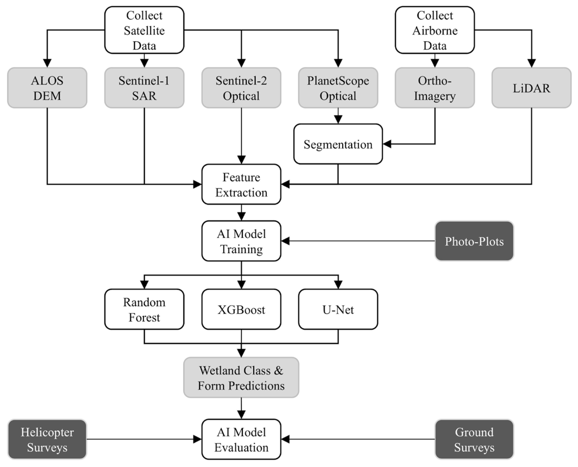
Several AI models were evaluated in this study. A generalized workflow is presented in Figure 3; however, inputs and algorithms varied depending on zone and pilot site. The following sections provide a detailed overview of the BFZ and PPZ AI modelling used for wetland mapping.

2.5.1. Boreal/Foothills Machine Learning

Building on recent boreal ML developments [59,82], a pixel-based Extreme Gradient Boosting (XGBoost) algorithm was chosen for BFZ ML modelling [83]. XGBoost is an ensemble learning method that groups together several “weak learner” decision trees to create a “strong learner”. This is performed sequentially, continuously correcting the previous weak learner until a final strong learner is achieved. Three XGBoost scenarios were tested for BFZ mapping. The first scenario included only important optical and SAR features, while the second and third scenarios used important features plus AW3D30 or LiDAR features. Identification and selection of important SAR and optical features followed methods in Merchant and McBlane [84]. This involved using the Shapley additive explanations (SHAP) algorithm, an explainable AI (XAI) method based on cooperative game theory [85]. SHAP values quantify the contribution of variables to a model’s prediction, allowing variables to be ranked by importance. The 20 most important features identified by SHAP were chosen as BFZ XGBoost model inputs, balancing predictive power and parsimony.
XGBoost models were developed using the Classification and Regression Training (caret) package in R. Training samples were randomly created using the enhanced ABMI 3 × 7 km photoplots. A balanced sampling design was used as this has been shown to produce accurate wetland mapping results with ML [86]. Three thousand points per class or form were created with a minimum of 10 m distance between points. This sampling procedure was repeated four times for each BFZ pilot, resulting in four unique training sets. Separate XGBoost models were trained using each training set, resulting in four class and form predictions. Predictions were summarized into a final classification by taking the mode of each prediction. It should be noted that ML form models were trained to map vegetation community (i.e., graminoid, shrubby, wooded, etc.). Therefore, to make a final form prediction, the vegetation community ML prediction was intersected with the preceding ML class prediction (e.g., if the ML class prediction was bog, and the vegetation community prediction was shrubby, then the form prediction would be shrubby bog). All XGBoost models were optimized by tuning key hyperparameters (e.g., max depth, nrounds, eta, and subsample) which control model complexity and behaviour, using an exhaustive grid search method and k-fold cross validation [87] with a total of 5 folds used for tuning. Model predictions were generated at 10 m spatial resolution, which meets the target 0.9 ha MMU.

2.5.2. Boreal/Foothills Deep Learning

BFZ wetland mapping with DL followed similar CNN methods developed by DeLancey et al. [44]. CNN modelling was implemented in Python using the Keras deep learning library. The CNN was based on a U-Net architecture [88], which is an encoder–decoder that performs image segmentation by producing an output with similar dimensions as the input. Input training patches were of size 224 × 224 pixels. Two U-Net scenarios with different inputs were tested for boreal mapping. Each scenario used the same optical and SAR features, but included either LiDAR or AW3D30 features. Only a minor number of features were discarded in each scenario since DL models can automatically learn relevant hierarchical features [89].
During initial stages of CNN model development, several notable observations were made: that different groups of feature inputs did not affect results as much as training regime, that aggressive data augmentation was the biggest factor for improvement, and that training cycles were short. This suggested that the CNN was data-starved. To address this, additional pseudo-plots were generated by producing weak labels from a baseline U-Net trained only on the enhanced 3 × 7 km photoplots. Pseudo-labelling approaches have proven effective in remote sensing studies [90]. The weakly labelled pseudo-plots expanded the training set and helped the U-Net learn general spatial patterns before later being fine-tuned with the expert labelled 3 × 7 km photoplots.
All U-Net models were developed using data from both Boreal-1 and Boreal-2 pilots, rather than performing pilot-specific training. This was due to the limited amount of label data, and the requirements of DL. U-Net base models were first trained using all pseudo-plots and all but four photoplots (i.e., holdouts), which were used for monitoring training progress. Patches were sampled with a window stride of 45, augmented using flipping and 90° rotations, and normalized. Certain wetland classes or forms were oversampled to account for rarity (e.g., bogs and marshes). Base models were trained for 50 epochs (200 iterations per epoch) with a batch size of 16 and an initial learning rate of 0.001, which was lessened to 0.0005 at the 40th epoch. These base U-Net models were then fine-tuned using only patches from photoplots, and not pseudo-plots. For fine-tuning, a tighter window stride of 10 was used with a learning rate of 0.0002, which decayed by a factor of two every six epochs. These fine-tuned models reached their minimum loss at around 20 epochs (100 iterations per epoch). The best fine-tuned U-Nets were chosen according to their loss performance on the holdout photoplots.
A summary of BFZ AI modelling scenarios is found in Table 3. These scenarios were tested for both wetland class and form mapping.

2.5.3. Prairie/Parkland Machine Learning

The PPZ pilots implemented object-based ML modelling. This allowed us to compare an existing operational Random Forest (RF) object-based image analysis (OBIA) method that uses a set of optimized RS variables (unpublished by DUC) against a novel XGBoost OBIA method. All segmentation processing was performed using PCI Object Analyst. OBIA models evaluated segmentations derived from both high-resolution (3 m) PlanetScope and very-high-resolution (1 m) orthophotography (i.e., aerial imagery). Following segmentation, numerous ML scenarios with different RS inputs were tested. This included various combinations of predictors, including optimized terrain and optical variables identified in the conventional DUC workflow, optimized PlanetScope variables, Sentinel-2 variables, or LiDAR variables which included either point cloud variables, topographic variables, or with or without the use of LevelSet. The effect of LevelSet was a particular focus in this work since it is capable of effectively mapping wetland depressions [91].
XGBoost OBIA models also underwent several additional, enhanced ML development steps. First, a training data selection method was employed using Gradient Information Optimization (GIO), which refines training data by minimizing divergence from a reference “pure” set while preserving information content [92]. GIO uses gradient descent and k-mean clustering to accomplish this. GIO was implemented to reconcile PPZ training data collected from different years and seasons, which posed a unique mapping challenge since PPZ wetlands are dynamic and vary in extent over time [93]. To collect the “pure” dataset for GIO, 100 OBIA segments were randomly selected and stratified by form. All segments needed to have at least 80% overlap with validated (i.e., truth) photoplot labels, although upland segments required additional screening due to their high landcover variability. This was performed by vetting upland segments against a PlanetScope derived water/non-water mask, in which segments needed to have an intersection over union (IOU) greater than the calculated median IOU. Once the pure dataset was compiled, GIO was implemented using the following parameters: cluster size of k = 1500, learning rate of 0.03, and maximum iteration size of 4000 for each form.
After generating a refined training dataset with GIO, a test dataset was then created by selecting a subset of segments with high IOU values, and that were spatially disjointed (i.e., did not overlap) from the GIO training dataset. Using the train and test datasets, 10 spatially independent k-folds were created with 1 km buffers. Conjointly, 10 stratified, non-spatial k-folds were created using a train–test split of 0.9 to 0.1. Both k-folds were then merged on the fold number, and upsampled to account for class imbalance. For ML scenarios that used orthophotography, segments used for training and k-fold creation needed to have 90% overlap with PlanetScope GIO segments.
All PPZ XGBoost models were tuned using Bayesian optimization and Parzen Tree Estimators (PTEs; [94]). PTE was chosen because of the large number of PPZ samples to train with. Bayesian optimization keeps track of past results to form probability mappings of hyperparameter combinations, making it a very efficient approach. PTE hyperparameter tuning used the Hyplot Python library. All predictor variables were used to establish a baseline, tuned model prior to variable selection.
After PTE tuning, variable selection was performed using a combination of SHAP values and Genetic Algorithms (GAs). GAs excel at handling large datasets and at finding solutions to optimization problems with many possible outcomes [95]. However, they are computationally intensive since each solution needs to be evaluated. To address this challenge, we leveraged SHAP values to simulate the predictions of a model in an efficient way. This was on the basis that SHAP values are distributed across predictors, and sum to the value of prediction across all variables—meaning if you add up all the SHAP values for a given prediction, you obtain the same result as the model’s actual prediction [96]. To verify this phenomenon, an XGBoost model was built with Parkland-1 training data using all RS variables and 150 model configurations. The predictions from each model configuration were compared to the predictions generated by the SHAP values. Comparing the results of each method produced an R2 of 0.83, suggesting good approximation with this technique. This finding allowed us to use GAs to perform variable selection, by using predictions estimated from SHAP values without needing to compute each model. For each model, the fit function was the resulting F1-score along with an L2 regularization-inspired penalization function, which helped stabilize accuracy. Once each model underwent variable selection, another tuning was performed with Hypopt using only the original k-folds.
The last component of PPZ ML modelling involved correcting XGBoost models using active learning. This was because initial model runs were overpredicting tilled marshes. We used the modAI Python package to implement ranked batch-mode active learning (RBMAL). RBMAL iteratively retrains a model by ranking unlabeled samples based on a composite acquisition score that balances model uncertainty and sample diversity. An uncertainty score for each class is recorded, derived from XGBoost class posterior probabilities, along with a diversity score computed to reduce redundancy among selected samples. These are combined to create a single composite score, using a weighted linear scoring function, with equal weighting applied to uncertainty and diversity (0.5), and used to rank all unlabeled points. RBMAL was used to select points out of a pool of incorrectly classified tilled marsh segments. A starting XGBoost model was created with 500 trees, max depth of 5, and learning rate of 0.05. Model retraining was then repeated for 500 iterations, using 10 points added during each iteration. The augmented training set was used as a template for further PPZ XGBoost models.

2.5.4. Prairie/Parkland Deep Learning

PPZ wetland mapping with DL was also based on a U-Net CNN. CNN modelling followed a two-stage training process. The first stage developed a base model U-Net trained on all photoplot labels, for all time periods. The second stage fine-tuned this model using only labels from 2023. This approach was taken because the most recent 2023 labels had considerably more detail. Thus, fine-tuning the PPZ U-Net encouraged the finer detail to be captured. However, it should be noted that 2023 label and validation data did not contain fen samples. As such, the U-Net was not fine-tuned with this class.
The base model U-Net was trained for 30 epochs (300 iterations per epoch) with a learning rate of 0.002 that halved at epoch 25. Input patches were sampled with a window stride of 45, augmented using flipping and 90° rotations, and normalized. The fine-tuned U-Net was trained for 20 epochs (200 iterations per epoch) with a learning rate of 0.0001 which halved each eight epochs. Patches were samples with a tighter 22 pixel stride, augmented using flipping and arbitrary rotations, and normalized. Both the base model and fine-tuned model used input patch sizes of 256 × 256. During training, loss and metrics were monitored after each epoch on a holdout 5 km2 area of training labels. This holdout was used to choose the best U-Net model.
A summary of PPZ AI modelling scenarios is found in Table 4. These scenarios were tested for wetland form mapping, but not class. This is because, unlike the BFZ, wetland diversity in the PPZ is very low. For example, in most cases, only one form existed per class in each pilot (e.g., graminoid marsh, shrubby swamp, bare open water). Therefore, it was more appropriate to model wetlands directly at the form level.

2.6. Accuracy Assessments

All AI models were evaluated using common mapping accuracy metrics [97]. This included overall map accuracy (OA), since this is the benchmark metric outlined by the GOA, as well per-class F1-score calculated from precision and recall:
Overall accuracy = Correctly classified pixels/total pixels
Precision = TP/TP + FP
Recall = TP/TP + FN
F1 = 2 × Precision × Recall/Precision + Recall
where TP, FP, and FN reflect the number of true positives, false positives, and false negatives, respectively.

2.7. Post Processing

A non-vegetated human footprint layer, pulled from the ABMI’s 2021 Human Footprint Inventory (HFI; [98]), was used to mask out disturbed areas as a post-processing step. This was performed for all pilots using the following HFI sublayers: reservoirs, borrow pits, non-permeable roads, rail lines, canals, mine sites, and industrial sites.

3. Results

3.1. Boreal/Foothills Modelling Results

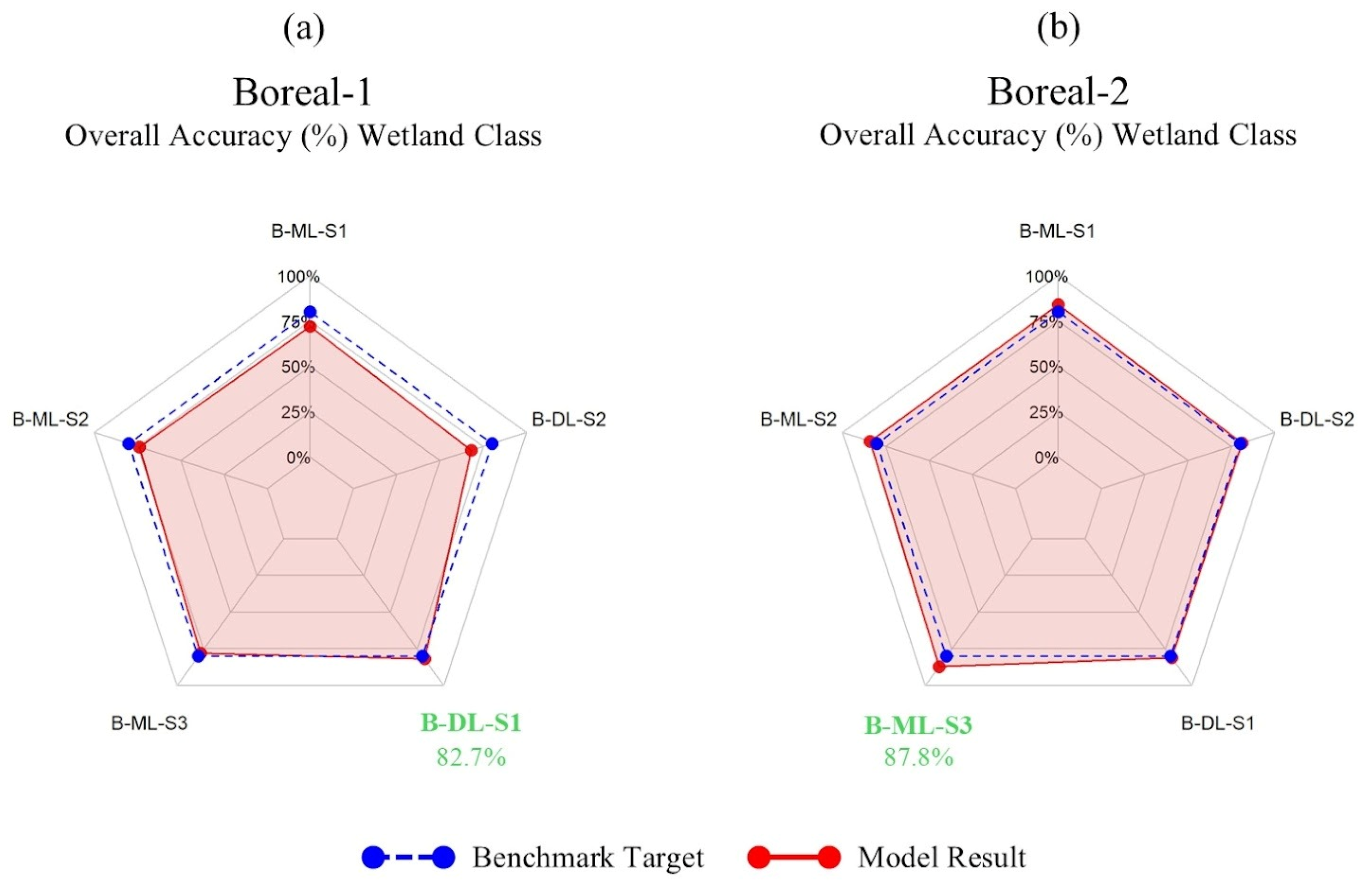
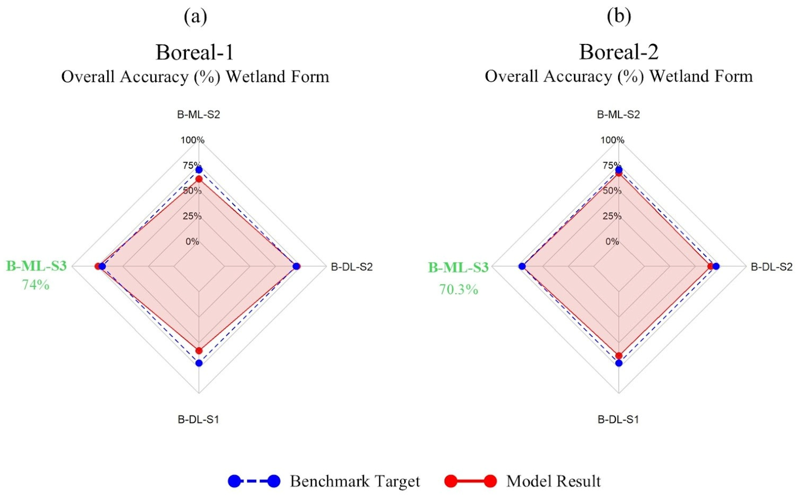
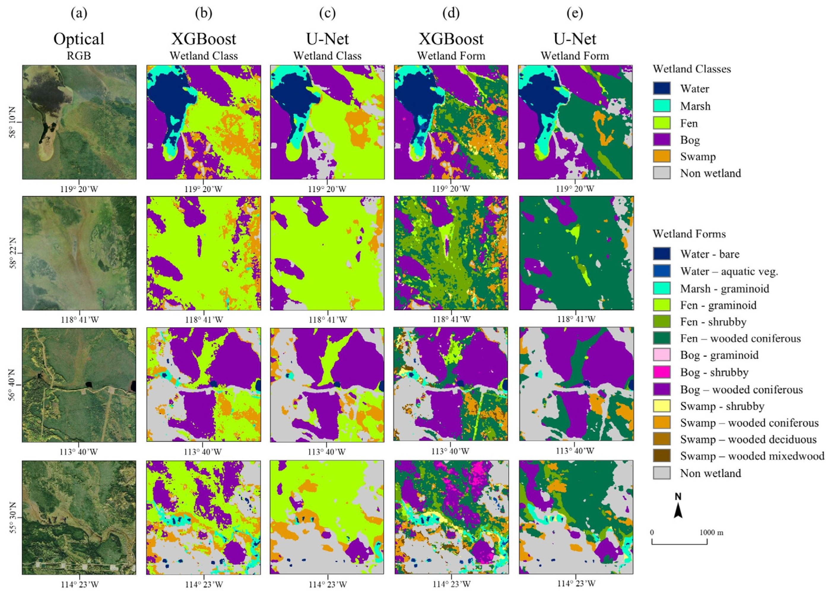
At the wetland class detail, the benchmark OA target of 80% set by the GOA [16] was met in both BFZ pilots. In Boreal-1, a highest OA of 82.7% was achieved with B-DL-S1, and in Boreal-2, a highest OA of 87.8% with B-ML-S3 (Figure 4; see Table 3 for scenario descriptions). B-DL-S1 was the only AI model scenario to exceed 80% OA at the class detail in Boreal-1, whereas in Boreal-2 all AI model scenarios exceeded 80% OA. At the wetland form detail, the benchmark OA target of 70% was also met in both BFZ pilots. In Boreal-1, a highest OA of 74% was achieved with B-ML-S3, and in Boreal-2, a highest OA of 70.3% was achieved also with B-ML-S3 (Figure 5). B-DL-S2 was the other AI model that exceeded 70% OA in Boreal-1, whereas in Boreal-2 only B-ML-S3 met the target OA.
The per-class F1-scores achieved by the best BFZ AI models are found in Table 5. F1-scores are reported for both class and form details. F1-scores varied considerably between and within classes, and across BFZ pilots. At the class level, F1-scores varied from 0.64 to 0.98 in Boreal-1, and 0.68 to 0.98 in Boreal-2. Water and upland classes were the highest F1-scores in both BFZ pilots. At the form detail, F1-scores varied from 0.26 to 0.95 in Boreal-1, and 0.04 to 0.96 in Boreal-2. In general, forms that are more rare, such as graminoid bogs or wooded mixedwood swamps, had lower F1-scores.
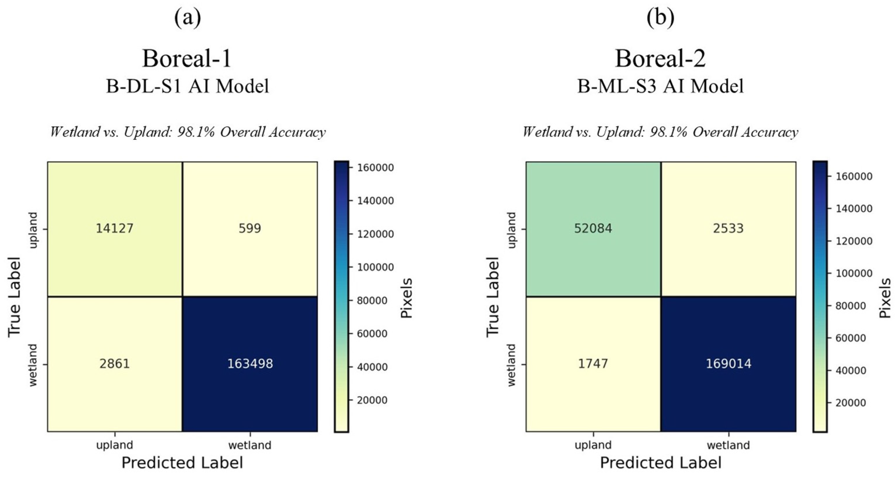
The performances of the best models for each BFZ pilot were further evaluated at the more general wetland/upland detail. An OA of 98.1% was achieved in both pilots at this binary detail, using the B-DL-S1 AI model in Boreal-2 and B-ML-S3 AI model in Boreal-2. This meets the 90% OA target set by the GOA. Error matrices found in Figure 6 show the confusion for these models, which indicate minimal commission (599, 2533) and omission (2861, 1747) errors between the general wetland and upland differentiation.

3.2. Prairie/Parkland Modelling Results

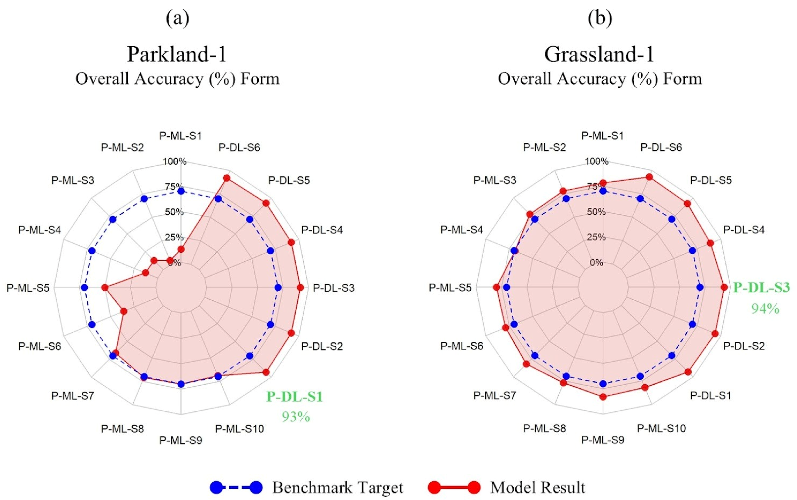
The OAs of PPZ models were evaluated directly at the form level, since wetland diversity was low and modelling was performed directly at this detail. The benchmark OA target of 70% was met in both PPZ pilots, and accordingly, the 80% OA class target was also met (Figure 7; see Table 4 for scenario descriptions). In Parkland-1, a highest OA of 93% was achieved with P-DL-S1, and in Grassland-1, a highest OA of 94% with P-DL-S3. All ML models based on the RF algorithm performed poorly relative to XGBoost and U-Net, especially in Parkland-1 where none of the RF models exceeded 70% OA. All DL models for both PPZ pilots achieved 89% OA or higher, although with the caveat that these models could not reliably predict fen wetlands in Parkland-1 (F1-scores of 0.00). P-ML-S9 was the most accurate ML model in Grassland-1, and P-ML-S8 in Parkland-1, with the latter capable of identifying fens.
The per-class F1-scores achieved by the best PPZ AI models are found in Table 6. F1-scores did not vary much between class and form, due to the low wetland diversity in each PPZ pilot—these areas are dominated by open water wetlands and marshes. For example, in Parkland-1, F1-scores for swamps and fens were very low, as these classes are scarcely represented. Bare water and graminoid marsh F1-scores ranged from 0.73 to 0.79 in Parkland-1, and 0.49 to 0.74 in Grassland-1. Tilled marshes were not reliably mapped by any DL model, which is notable since some ML models were able to predict this minority form. Uplands were mapped with high accuracy in both pilots, achieving F1-scores of 0.97.
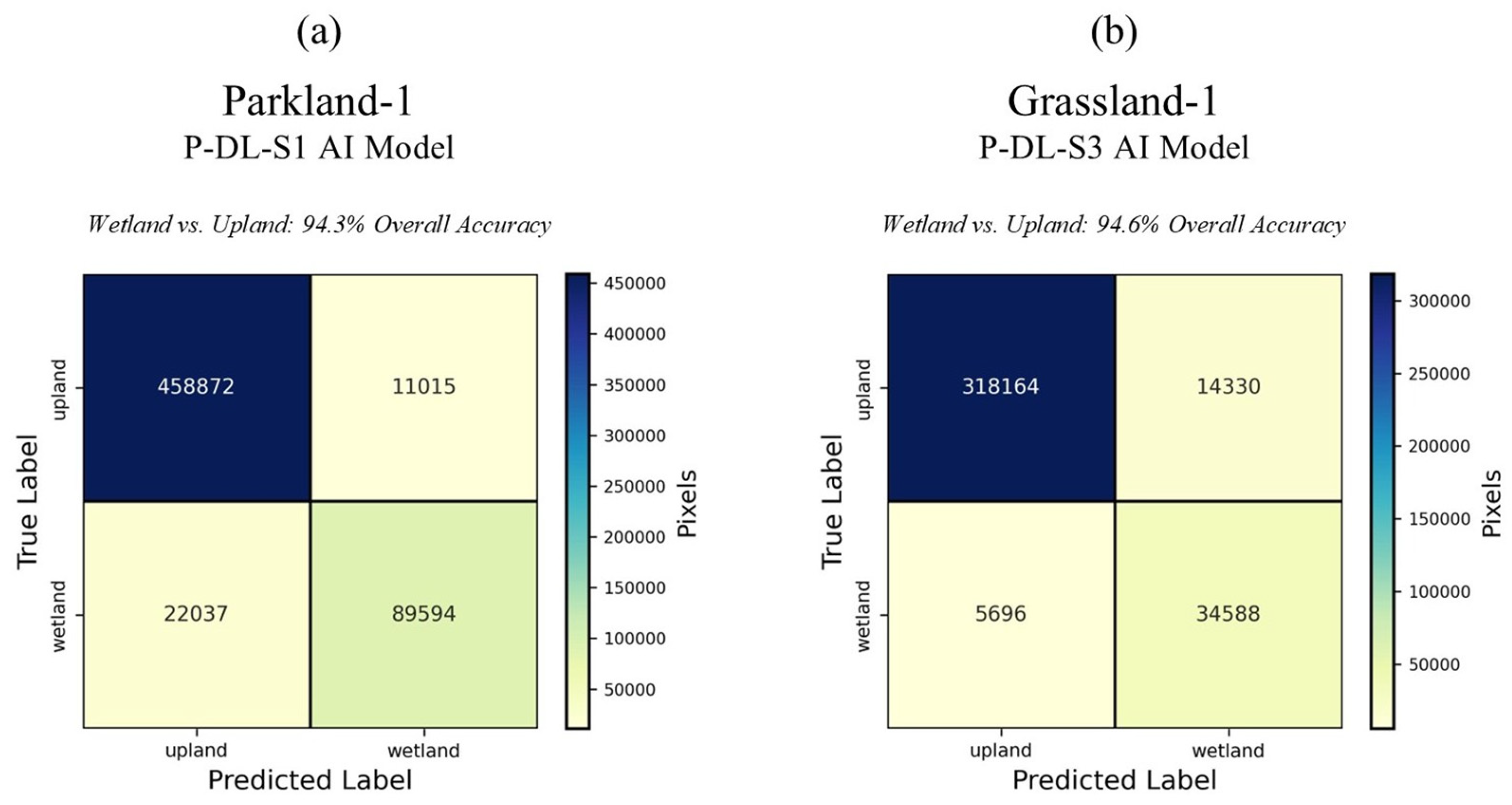
When evaluated at the more general wetland/upland classification level, the best-performing models achieved OAs of 94.3% in Parkland-1 and 94.6% in Grassland-1, exceeding the 90% OA target. The corresponding error matrices, which also highlight very little omission (22,037, 5,696) and commission (11,015, 14,330) errors, are presented in Figure 8.

4. Discussion

4.1. Analysis of Boreal/Foothills AI Experiments

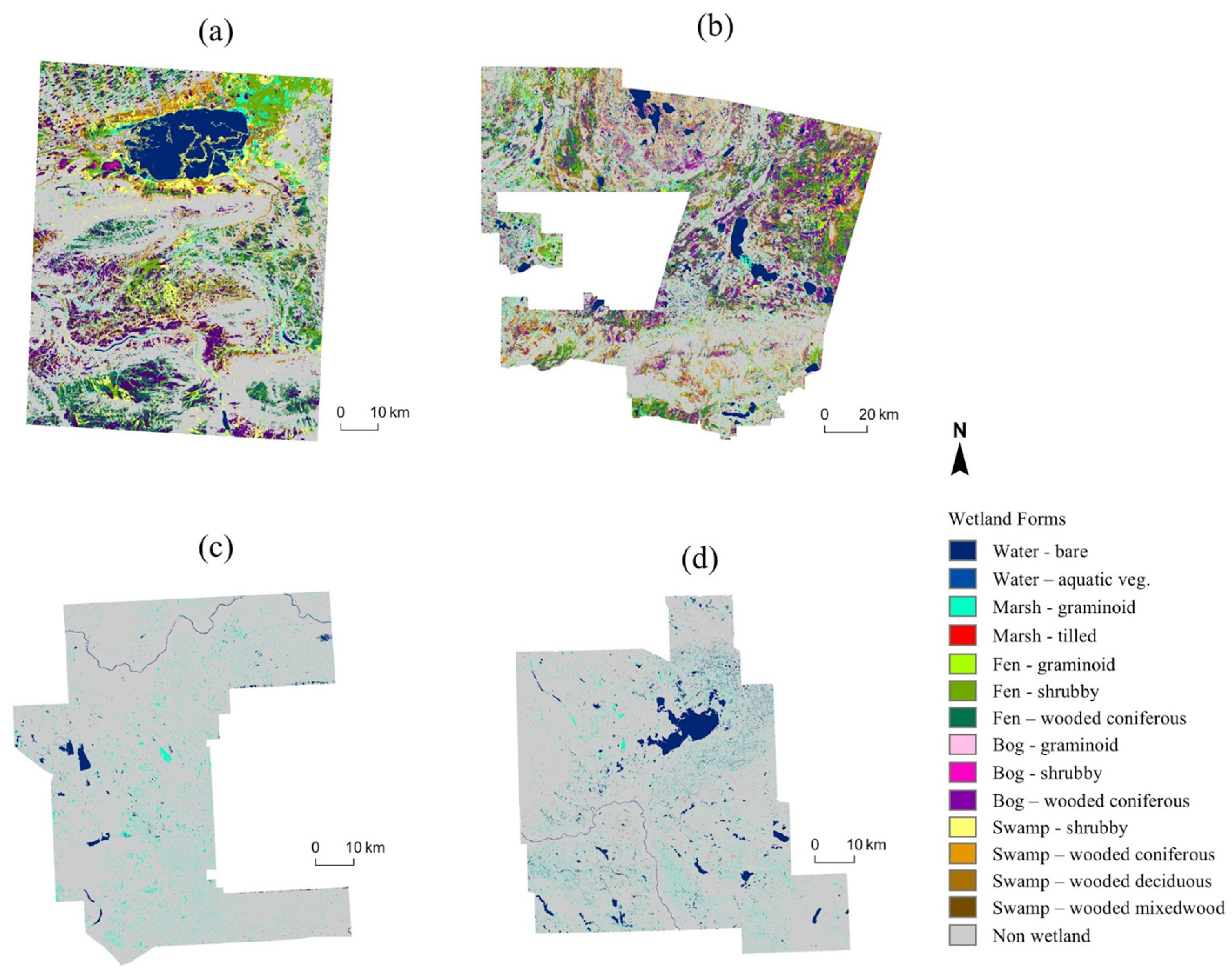
Our experiments indicated that AI-based modelling can meet the GOA BFZ mapping standards, including target classification detail, accuracy, and MMU (see Figure A2 Appendix A for final BFZ wetland inventory maps). ML modelling with XGBoost produced the best results for form-level mapping in Boreal-1 and Boreal-2, using the B-ML-S3 scenario. This ML scenario integrated satellite imagery and LiDAR derivatives, and represented significant OA increases (3–12%) compared to B-ML-S2 which used the AW3D30 DSM topographic data. Similarly, the inclusion of LiDAR also elevated all DL models for form-level mapping (2–13% OA increases). No ML or DL scenario was able to achieve the 70% OA form-level target without the use of bare earth LiDAR. This finding can be attributed to the higher spatial resolution and quality of airborne LiDAR DTM data, which are capable of preserving important wetland features that manifest from topographic variations [99,100]. LiDAR can also capably separate and characterize vegetation layers that define wetland forms and their communities, by deriving ecologically relevant 3D structural information [101]. This high-resolution, LiDAR-derived information has proven valuable for wetland form mapping in Alberta in other studies [102].
The BFZ pilot results also highlight the effectiveness of ML over DL for detailed wetland form mapping, which we attribute to the rarity of several wetland forms, the fine-scale variability in vegetation communities, and the available reference training dataset. DL models typically require large training datasets, which can make high-thematic resolution mapping challenging with limited samples, and even unsuccessful in some tasks or regions [103]. For instance, several BFZ wetland forms, such as wooded mixedwood swamps and graminoid bogs in Boreal-2, were present but very rare. After modelling, these rare forms were entirely missed by B-DL-S2 (F1-scores of 0.00). Despite applying aggressive DL data augmentation to address class imbalance [104], ML remained more effective for form-level mapping in the BFZ pilots. This aligns with prior studies showing that ML can sometimes outperform DL when sample sizes are limited [105]. El Bilali et al. [106], for example, found XGBoost superior to a DL neural network for RS image analysis, and attributed performance differences to dataset limitations which restricted the DL model’s ability to capture non-linearity. Additionally, Southworth et al. [107] provided a comprehensive review of DL versus ML for land cover classification applications, and found that higher accuracies with DL are not always substantial, nor are they always guaranteed. In fact, the authors identify many studies where ML classification accuracies surpassed DL, noting that the choice in AI algorithm should strongly consider factors such as training data size and RS imagery type.
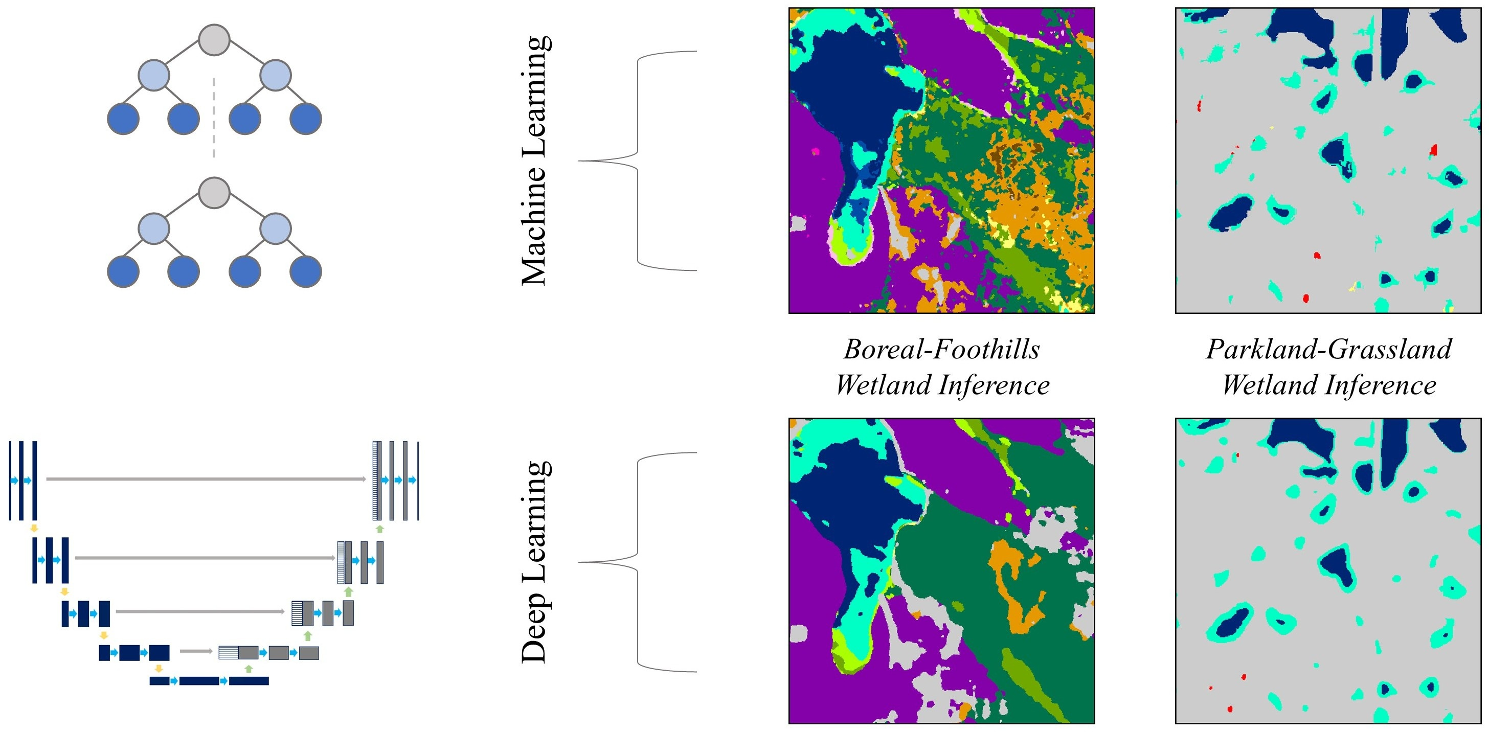
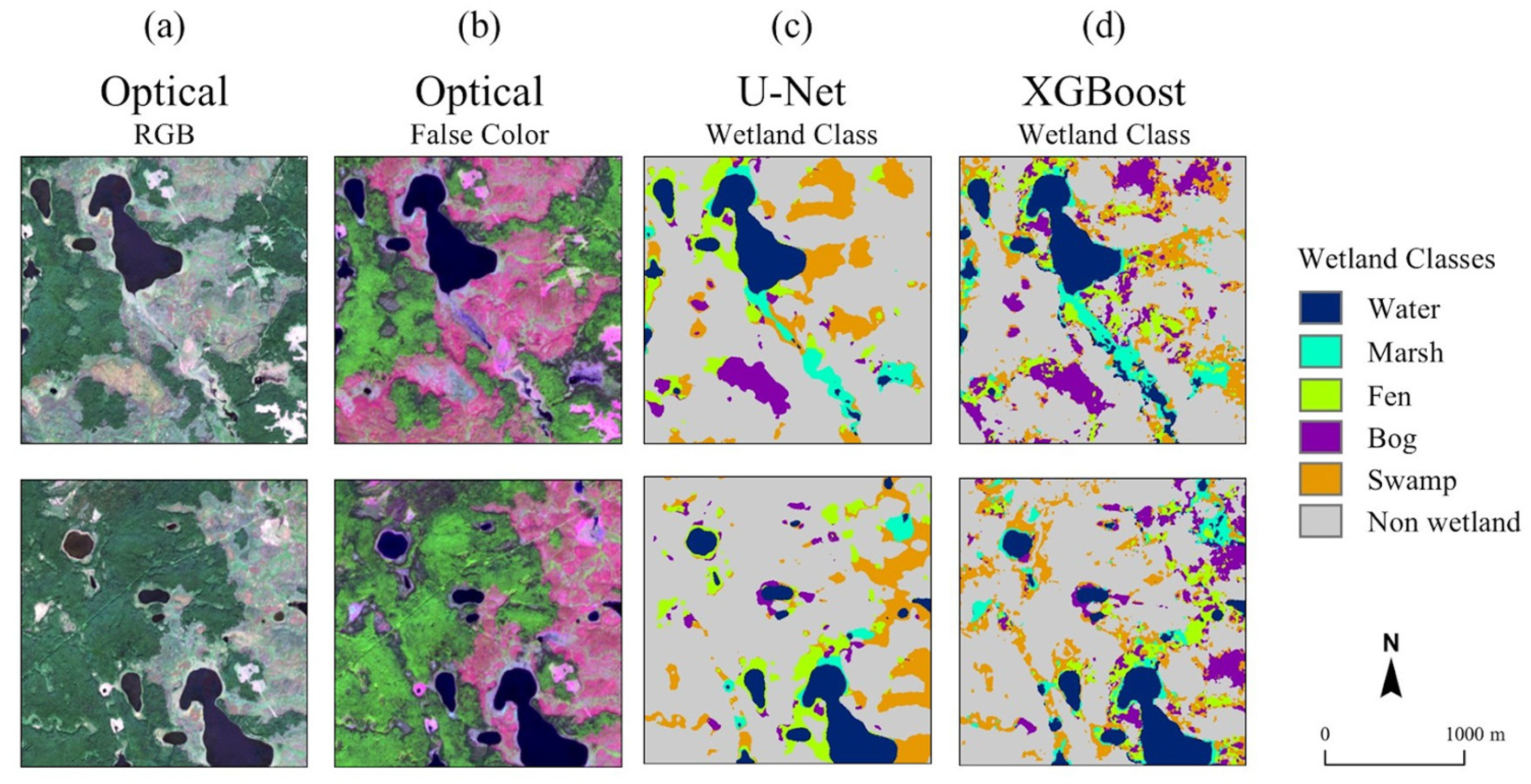
It is known that DL models tend to sacrifice fine granular details in order to achieve higher performance, and instead focus on more prominent features [108]. This is because the architecture of DL CNNs, like U-Net, are designed to learn high-level features and contextual information very well [109]. The convolutional filters and the pooling processes of CNNs, which are lossy [110], act as edge detectors and tend to produce smooth, coherent outputs which lack “salt-and-pepper” type noise that is more common with ML outputs [111]. An example of this is presented in Figure 9, where predictions from the best ML and DL models are visually compared. At the class level, where wetlands display broader spatial patterns with more distinct boundaries and edges, DL generally demonstrated more favourable performance. Evidently, the aggregation and smoothing processes of U-Net are more effective at this wetland class level, where there is less local and fine-scale variability. Delancey et al. [44] found a similar result when comparing U-Net and XGBoost for class level wetland mapping in northern Alberta, whereby the former produced smoother and more accurate predictions. In the current study, the B-DL-S1 scenario achieved the class level OA target (80%) in both Boreal-1 and -2 pilots, whereas no ML scenario met this target in Boreal-1. However, at the generalized wetland–upland level, both ML and DL demonstrated remarkable performance (98.1% OA), with little omission or commission error between wetlands and non-wetlands.

4.2. Analysis of Prairie/Parkland AI Experiments

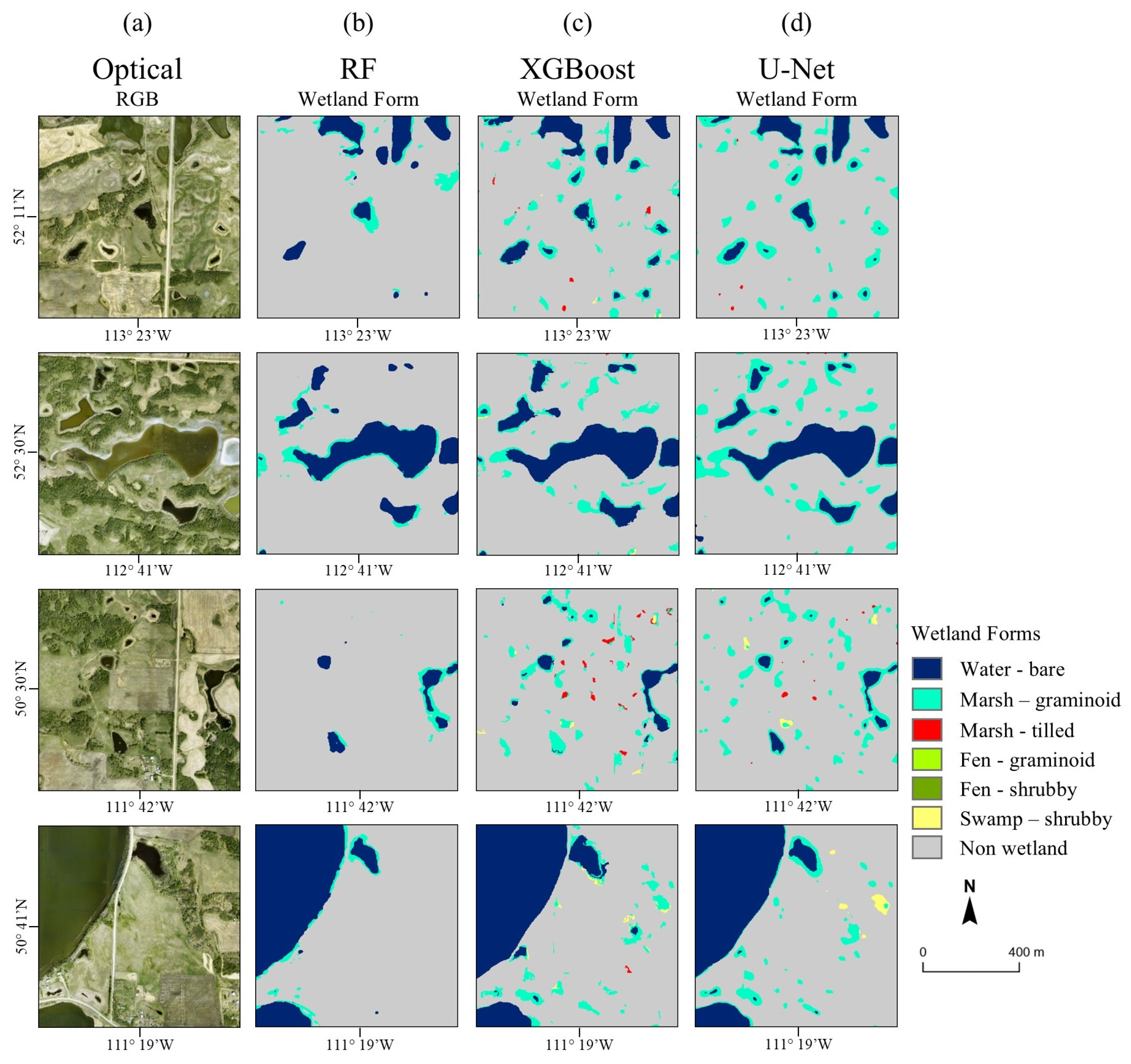
Similarly to the BFZ pilots, AI-based modelling met the minimum mapping standards in both the Grassland-1 and Parkland-2 PPZ pilots, and even exceeded the required classification detail by mapping to wetland form detail, despite the provincial mandate specifying only class-level detail ([16]; see Figure A2 Appendix A for final PPZ wetland inventory maps). The highest-performing AI models also achieved accuracies well above provincial targets at the wetland (90%), class (80%), and form (70%) details (Figure 10). DL modelling with U-Net produced the best overall accuracy results at the form detail in both PPZ pilots, although with some notable caveats compared to XGBoost ML models, which are discussed later in this section. In both PPZ pilots, OBIA models using RF yielded underwhelming results, consistent with recent wetland mapping studies that show traditional approaches, while easy to implement and computationally efficient, are consistently outperformed by more advanced and contemporary AI-based methods [112]. In Parkland-1, the best-performing scenario was P-DL-S1, which integrated all available PlanetScope, orthophotography, and LiDAR-derived variables. In Grassland-1, P-DL-S3 performed best, which used similar inputs but excluded CHM and LiDAR intensity. These findings underscore the value of high-resolution topographic inputs for wetland characterization in the PPZ [113,114,115]; however, the contribution of specific topographic variables varies with landscape context. For instance, depression probability and position index metrics show consistently strong associations with PPZ wetland occurrence [116,117], while canopy-related variables (e.g., CHM) are less informative in areas like Grassland-1 where wetland form diversity is limited, but become more valuable in regions with denser vegetation (i.e., from swamps, vegetated peatlands, etc.) that obscures underlying hydrology, such as in Parkland-1. Both DL models also benefited from the inclusion of seasonal PlanetScope imagery and high-resolution orthophotography. Seasonal imagery was particularly important given the highly dynamic nature of PPZ wetlands, which often experience spring flooding and fall drying [118,119,120]. These seasonal dynamics make PPZ wetlands challenging to map using single-date satellite or aerial imagery [121]. Moreover, orthophotos enhanced the DL model’s ability to precisely delineate wetland boundaries, particularly for the many small depressional wetlands (<1 ha) that are common across the PPZ [122].
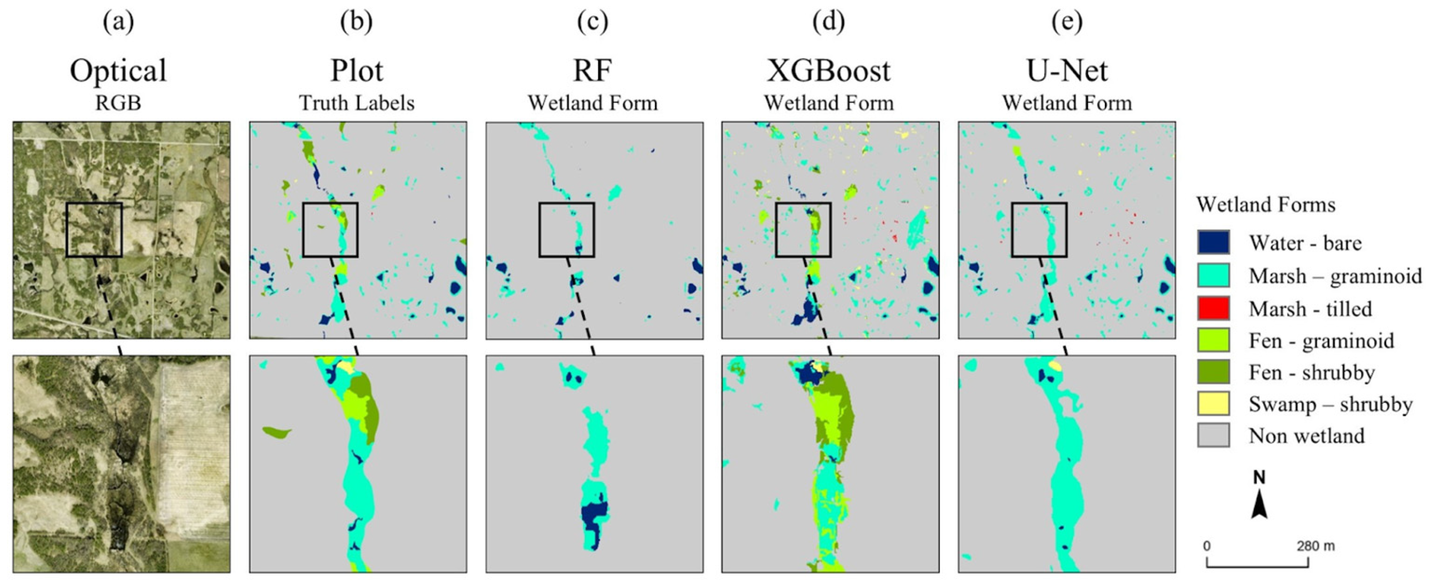
Despite achieving higher overall accuracies than both ML approaches (i.e., XGBoost and RF), DL models were less effective at mapping rare wetland forms such as fens and swamps. Prairie landscapes often contain extensive wetland cover, but this is typically open water and marshes [123]. CNN-based DL architectures, such as U-Net, are well-suited for learning dominant spatial patterns and therefore tend to generalize well on majority classes, often at the expense of underrepresented ones [104]. This poses challenges for real-world applications, such as operational wetland inventory development with highly imbalanced training data. For example, in Parkland-1, which is closer to the prairie–boreal transition zone and includes some peatland coverage (e.g., shrubby and graminoid fens), the best-performing DL model produced poor per-class F1-scores for these minority forms, both during the modelling validation stage and when compared against field-based reference data. In contrast, the best-performing ML model, P-ML-S8, achieved much higher fen F1-scores in the model development validation stage (e.g., >0.8 for both shrub and graminoid fen forms), and its final predictions aligned better when qualitatively assessed against high-resolution imagery. As such, the XGBoost ML approach produced more spatially realistic peatland distribution estimates across Parkland-1. Figure 11 illustrates this contrast, showing how only the XGBoost-based P-ML-S8 model accurately captured the presence of rare wetland types in a diverse training block, including fens and mixed marsh (e.g., graminoid and tilled). As in the BFZ experiments, this reinforces the adaptability and robustness of ML models to class-imbalanced training datasets, which is an area in which DL continues to experience challenges, particularly for minority class detection [124]. Notably, in more homogeneous landscapes such as Grassland-1, where wetland diversity is lower, DL models excelled with strong performances.

4.3. Study Implications and Recommendations for Provincial Wetland Inventory Mapping

Alberta is home to a vast and diverse array of wetlands. Recognizing their ecological and societal value and the high losses of wetlands due to historical and continued population growth and human pressures, the provincial government has adopted the Alberta Wetland Policy and associated Wetland Replacement Program. The implementation of the policy requires accurate, up-to-date, and spatially explicit information on wetland extent and type to support regulatory, conservation, and monitoring applications [6,9,12,13,125]. Motivation for this study stemmed from the need to modernize Alberta’s wetland inventory using scalable, repeatable, and cost-effective methods that can support ongoing regulatory, management, and conservation needs. Traditional inventory approaches, such as manual air photo interpretation and field-based mapping, while accurate at local scales, lack the efficiency and repeatability needed for consistent province-wide wetland mapping and monitoring updates. The results of this study demonstrate that modern, AI-driven RS approaches, particularly those integrating EO imagery, high-resolution LiDAR, and ML or DL can meet and even exceed the provincial standards for wetland classification accuracy, detail, and MMU. These methods offer a practical path toward operationalizing wetland inventory updates at scale.
However, this study also highlights several important nuances. Scaling these approaches across the province will require careful consideration of regional wetland characteristics, the availability of RS data, and the efficacy and relative return on investment of different AI technologies. As such, implementation strategies should weigh both the ecological complexity of the target biome and the cost-effectiveness of the chosen AI modelling approach and its imagery inputs [126].
Based on the results of this study, we provide the following region-specific recommendations to support the scalable implementation of wetland inventory mapping across Alberta, with separate considerations for BFZ and PPZ.
In the BFZ, recommendations stemming from this study include the following:
  • Contributions of LiDAR: LiDAR proved effective in meeting wetland form mapping accuracy targets in the BFZ pilots. Terrain and canopy structure variables were essential for capturing wetland features that manifest from topographic variation, consistent with findings from a broad body of the scientific literature [127]. Given that much of the province’s managed boreal forest area already has, or is planned to receive, high-resolution LiDAR coverage (e.g., from industry, non-governmental organizations, etc.), we recommend that future BFZ wetland inventory efforts incorporate LiDAR-derived inputs to support consistent wetland classification at finer thematic detail (i.e., form).
  • Reference data: Field reference datasets are strongly recommended to support AI modelling development and optimization, and to account for subtle hydro-ecological distinctions not easily determined by RS alone. Helicopter-based sampling is particularly favourable for remote area access in the boreal forest, but should be complemented by targeted ground-based surveys to capture critical wetland attributes (e.g., peat depth). Supplementing field campaigns with high-resolution photo interpretation and historical datasets (e.g., photoplots) is also a viable approach, but requires expert validation and quality control. A combined strategy that integrates field, historical, and photo-interpreted data offers a practical balance of quality, feasibility, and spatial coverage for training and validation purposes in the BFZ.
  • AI modelling: Both ML and DL approaches performed well in the BFZ pilots, producing ecologically meaningful wetland classifications. U-Net’s strength lies in its ability to produce smooth and coherent wetland class boundaries, while XGBoost excelled at mapping more rare wetland classes (i.e., bogs) and capturing finer form-level granularity and vegetation communities. However, U-Net likely holds greater long-term performance potential as more training and enhanced photoplot data become available. As such, both AI technologies may inform future inventory updates, but DL may consistently surpass ML as data quality and coverage increases.
In the PPZ, recommendations stemming from this study include the following:
  • Contributions of LiDAR: Topography is a major driver of wetland presence in the PPZ, making the inclusion of LiDAR data a priority for any future inventory updates. While the contribution of specific LiDAR derivatives varied across PPZ pilots, terrain-based metrics (e.g., probability of depression) proved highly effective—these LiDAR variables were consistently retained as key model inputs following feature selection and optimization. Importantly, alternative open-source DEMs, which have only moderate horizontal and vertical accuracy, are known to be inadequate in characterizing PPZ depressions due to the relatively small size and subtle relief of PPZ wetlands [128]. However, high-resolution LiDAR is not widely available in the Prairie and Parkland areas of Alberta, like it is in the boreal, and these acquisitions are expensive, which is a key challenge for scaling up this approach. Further work is needed to develop cost-sharing strategies to fund high-resolution LiDAR acquisitions for wetland mapping.
  • Contributions of high-resolution satellite imagery: Satellite imagery at 3 m resolution is recommended for PPZ wetland inventories, as it provides sufficient granularity for AI models while avoiding the operational challenges and high costs of acquiring airborne imagery across large areas. Platforms with frequent repeat cycles, such as PlanetScope, offer a practical and scalable solution for provincial mapping programmemes.
  • Reference data: As in the BFZ, quality training and validation data remain critical. However, operational constraints must be considered. Reliance on newly acquired aerial imagery introduces seasonality challenges, while end-to-end photogrammetric data (i.e., 3D generated photoplots) remain a gold standard but is often cost-prohibitive for larger projects. A shift toward 2D labelling using recent orthophotos or high-resolution satellite imagery is recommended to increase flexibility and scalability. Moreover, plot labelling should be cognizant of temporary, ephemeral wetlands. DL models (e.g., U-Net) are generally more tolerant of label variability in large, lower-quality datasets, whereas ML models like XGBoost require higher label accuracy but can more effectively leverage historical data. Regardless of the AI approach, the underrepresentation of minority wetland classes (e.g., fen, swamp) remains a concern. Targeted field sampling in areas of higher minority class occurrence can help address this imbalance and support more strategic, efficient field programme design.
  • AI modelling: In the PPZ, DL achieved the highest overall accuracies but struggled to detect and realistically predict minority wetland classes. ML, particularly XGBoost, outperformed DL in mapping less common wetland types such as fens, highlighting its effectiveness under class-imbalanced training conditions. This suggests that ML approaches may be better suited for operational wetland mapping in areas with greater form diversity. Conversely, U-Net demonstrated strong performance in delineating dominant wetland classes (e.g., marshes, open water). Given these trade-offs, a hybrid strategy that combines the precision of DL for majority classes with the sensitivity of ML for minority forms is recommended for optimal wetland inventory development in Alberta’s PPZ.

4.4. Study Limitations and Future Work

Future efforts would benefit from incorporating a hydroperiod-based approach (i.e., wetland inundation patterns), particularly in the PPZ, given the importance of water presence and duration dynamics in characterizing PPZ wetlands [120,129]. Hydroperiod information may help refine classification outcomes, especially for ephemeral water bodies which are difficult to detect using standard mapping methods [130]. High accuracy hydroperiod mapping of permanent and semi-permanent open water wetlands would help identify public-owned water bodies on private land. These waterbodies are not accurately mapped and require extensive field and GIS work to accurately identify and delineate these wetlands currently. However, generating accurate hydroperiod maps poses its own challenges. The high-frequency, high-resolution imagery (e.g., PlanetScope) needed to capture the fine temporal dynamics of small PPZ wetlands can be cost-prohibitive at scale. On the other hand, open-access sources such as Sentinel-1 and Sentinel-2 offer broader accessibility but lack the spatial and temporal resolution required to track small or short-lived wetlands [33]. This trade-off must be carefully considered.
In the BFZ pilots, active wildfire activity during the 2023 summer field season posed logistical constraints on ground-truth data collection. For instance, approximately 50% of Boreal-1 burned in 2023. Consequently, some areas within the boreal study regions had lower densities of newly collected validation data. This uneven sampling may have influenced AI model accuracy assessments, potentially skewing performance metrics in favour of better-sampled zones [131]. To best account for this, field crews adapted sampling plans in real time and supplemented data gaps with historical, archived surveys. However, future validation campaigns, especially those supporting operational inventory development, must account for the increased frequency and extent of wildfires in Canada’s boreal zone [132], with field protocols that are flexible yet spatially representative.
Natural disturbances such as wildfires can impact wetland classification accuracy and reduce mapping confidence [133]. In this study, both ML and DL models qualitatively performed well in mapping BFZ wetlands within burned areas, exhibiting low noise and minimal confusion (Figure 12). This is attributed in part to the integration of high-resolution bare earth LiDAR, which preserved topo-structural and hydrological features despite fire disturbance, and to the inclusion of intersecting photoplot data that provided wetland training samples over burned areas. These elements enabled the AI models to better learn the spectral characteristics of burned wetlands [134]. However, future research should more rigorously assess model performance in burned areas, particularly the influence of burn severity on wetland classification accuracies.
This study focused on method development in the BFZ and PPZ regions of Alberta, where provincial wetland mapping standards are well-established. In contrast, no dedicated standards currently exist for the Boreal Transition Zone (BTZ) or Rocky Mountain Natural Region. These regions are influenced by complex mountain topography or represent ecotonal zones blending prairie and boreal features, making wetlands there particularly challenging to classify. Evaluating existing AI models or developing tailored approaches for these regions, supported by additional pilot areas, would not only improve model sensitivity to diverse landscapes but also enhance training data coverage, facilitating scaling up to a comprehensive provincial wetland inventory.
Lastly, a key limitation of this study is the lack of water depth information (i.e., bathymetry), since only wetland surface extent was mapped. However, depth is a critical variable for differentiating shallow open water wetlands from deeper systems such as lakes. There are new and emerging satellite-based approaches for regional bathymetry mapping [135,136], but their applicability in Alberta remains uncertain. Future research should test and potentially integrate these scalable methods to better characterize and inform open water wetland classification.

5. Conclusions

This study evaluated the potential of AI-based methods for wetland mapping in the BFZ and PPZ regions of Alberta, Canada. The overall objective was to assess whether advanced ML and DL architectures could meet the provincial wetland mapping standards with respect to classification detail, accuracy, and MMU. A particular emphasis was placed on integrating high-resolution LiDAR data into the AI pipelines to evaluate its contribution to model performance. The results demonstrated that the top-performing AI models met and exceeded provincial standards, achieving over 70% overall accuracy in mapping wetland form detail across all pilots. These methods offer several advantages for operational wetland inventory development: they can efficiently process large volumes of RS data, learn complex spatial patterns, continuously improve with the incorporation of additional training data over time, and produce consistent, repeatable classifications. Compared to traditional photogrammetric approaches, AI-based methods are also more scalable, cost-effective, and less reliant on individual interpreter decisions. DL was shown to be highly effective for wetland mapping, yet data hungry, which has been shown in other studies. This study showed that high-resolution LiDAR across the study areas and high-resolution satellite imagery in the PPZ boosted accuracy, but are expensive to acquire, which is a key challenge in scaling up this approach in the PPZ. This study will inform future wetland inventory updates and wetland monitoring across the province of Alberta.

Author Contributions

Conceptualization, M.A.M., J.E., R.E., L.B., J.S., C.N.M., J.N.H., J.D., D.C., N.S., A.C., M.T.-R. and C.M.; methodology, M.A.M., J.E., R.E., L.B., J.S., D.C., N.S., A.C., M.T.-R., M.N., C.M. and K.M.; software, M.A.M., J.E. and J.S.; validation, M.A.M., J.E., R.E., L.B., J.S., J.D., D.C., A.C., M.N., C.M. and K.M.; formal analysis, M.A.M., J.E., R.E., L.B. and J.S.; investigation, M.A.M., J.E., R.E., J.S. and J.D.; resources, C.N.M., J.N.H., L.B. and D.C.; data curation, M.A.M., J.E., L.B., R.E. and T.D.; writing—original draft preparation, M.A.M., J.E., R.E., J.S. and L.B.; writing—review and editing, M.A.M., J.E., R.E., L.B., J.S., C.N.M., J.N.H., J.D., T.D., S.T., D.C., N.S., A.C., M.N., C.M., K.M. and M.T.-R.; visualization, M.A.M., J.E. and R.E.; supervision, L.B., C.N.M. and J.N.H.; project administration, L.B., C.N.M., J.N.H., S.T. and A.C.; funding acquisition, L.B., C.M., J.N.H., D.C. and A.C. All authors have read and agreed to the published version of the manuscript.

Funding

This work was funded by the GOA-EPA through the Wetland Replacement Program. This work was completed by the GOA-EPA through a contractor, DUC, and a subcontractor, the ABMI (Contract 23LND849). Environment and Climate Change Canada funded the air photo acquisition in the PPZ regions.

Data Availability Statement

The results from this study are hosted at the following web link: https://open.alberta.ca/opendata/gda-6b83b31a-fa66-4fba-8469-d29a5ef952b4#summary (accessed on 20 November 2025).

Acknowledgments

We gratefully acknowledge the various field, modelling, supervision, and funding support that made this work possible. This includes the field, technical, and management teams of the ABMI and DUC, and the GOA-EPA team that oversaw the overall project. We would like to thank Jim Herbers, Thorsten Hebben, Alain Richard, and Lindsay McBlane. Membership of the GOA-EPA team included the co-authors and the following individuals: Angela Burkinshaw, Erin Grass, Courtney Kelly, Josh Montgomery, Vanessa Swarbrick, and Jonathan Thompson. A special thank you to all those GOA-EPA individuals.

Conflicts of Interest

The authors declare no conflicts of interest.

Appendix A

Table A1. Summary of remote sensing datasets used for BFZ wetland modelling.
PlatformDate TypeSpatial ResolutionAcquisition YearsSeasonal Composites
Sentinel-2Optical10–20 m2020–2022Early (June–July) and Late (August–September)
Sentinel-1SAR10 m2020–2022Early (June–July) and Late (August–September)
LiDARTopographic1 m2021–2022-
AW3D30Topographic30 m2006–2011-
Table A2. Overview of BFZ LiDAR sources, coverage, and derivatives.
Pilot NameProviderYearPoint Density (Points/m2)Coverage (km2)Derivatives
Boreal-1Tolko2022166583DEM, CHM, intensity, TWI, TPI, TRI, VBF
ABMI2022121050
Boreal-2Alberta-Pacific2022129703
West Fraser202117–3011,428
Table A3. Summary of remote sensing datasets used for PPZ wetland modelling.
PlatformDate TypeSpatial ResolutionAcquisition YearsSeasonal Composites
Sentinel-2Optical10–20 m2023Early (May) and Late (July–August)
PlanetScopeOptical3 m2023Early (April) and Late (July)
OrthoimageryOptical0.25 m2023Early (May) to Late (September)
LiDARTopographic1 m2022-
Table A4. Overview of PPZ LiDAR sources, coverage, and derivatives.
Pilot NameProviderYearPoint Density (Points/m2)Coverage (km2)Derivatives
Parkland-1GOA202265170DEM, slope, CHM, intensity, TPI, LevelSet, PDEP, DDME, DDSE
Grassland-1GOA202265065
Table A5. Summary of field survey sites (polygons) collected for each pilot.
ClassFormBoreal-1Boreal-2Parkland-1Grassland-1
WaterBare325613
Aquatic vegetation0234
MarshGraminoid3938332101
Tilled00057
FenGraminoid46300
Shrubby223400
Wooded coniferous194300
BogGraminoid01900
Shrubby0700
Wooded coniferous327500
SwampShrubby4058200
Wooded coniferous83300
Wooded deciduous212100
Wooded mixedwood71700
UplandUpland22734527
Table A6. Summary of ABMI 3 × 7 km photoplot review and correction process, comparing the number of polygons prior to review, and after.
Boreal-1Boreal-2
ClassOriginalAfter ReviewOriginalAfter Review
Water9964491347
Marsh37100278432
Fen36731526222437
Bog641076131149
Swamp20943924232544
Upland1534128584247941
Figure A1. Location of reference data collected for each pilot. (a) Boreal-1. (b) Boreal-2. (c) Grassland-1. (d) Parkland-1.
Remotesensing 18 00507 g0a1
Figure A2. Final wetland inventories derived from the most accurate AI models for each pilot. (a) Boreal-1. (b) Boreal-2. (c) Grassland-1. (d) Parkland-1.
Remotesensing 18 00507 g0a2

References

  1. Xu, X.; Chen, M.; Yang, G.; Jiang, B.; Zhang, J. Wetland Ecosystem Services Research: A Critical Review. Glob. Ecol. Conserv. 2020, 22, e01027. [Google Scholar] [CrossRef] [Scilit]
  2. Fluet-Chouinard, E.; Stocker, B.D.; Zhang, Z.; Malhotra, A.; Melton, J.R.; Poulter, B.; Kaplan, J.O.; Goldewijk, K.K.; Siebert, S.; Minayeva, T.; et al. Extensive Global Wetland Loss over the Past Three Centuries. Nature 2023, 614, 281–286. [Google Scholar] [CrossRef] [Scilit]
  3. Tozer, D.C.; Steele, O.; Gloutney, M. Multispecies Benefits of Wetland Conservation for Marsh Birds, Frogs, and Species at Risk. J. Environ. Manag. 2018, 212, 160–168. [Google Scholar] [CrossRef] [Scilit]
  4. De Waard, F.; Connolly, J.; Barthelmes, A.; Joosten, H.; van der Linden, S. Remote Sensing of Peatland Degradation in Temperate and Boreal Climate Zones—A Review of the Potentials, Gaps, and Challenges. Ecol. Indic. 2024, 166, 112437. [Google Scholar] [CrossRef] [Scilit]
  5. Moomaw, W.R.; Chmura, G.L.; Davies, G.T.; Finlayson, C.M.; Middleton, B.A.; Natali, S.M.; Perry, J.E.; Roulet, N.; Sutton-Grier, A.E. Wetlands in a Changing Climate: Science, Policy and Management. Wetlands 2018, 38, 183–205. [Google Scholar] [CrossRef] [Scilit]
  6. Clare, S.; Creed, I.F. Tracking Wetland Loss to Improve Evidence-Based Wetland Policy Learning and Decision Making. Wetl. Ecol. Manag. 2014, 22, 235–245. [Google Scholar] [CrossRef] [Scilit]
  7. Alberta Environment and Parks. Alberta Merged Wetland Inventory Class; Geodatabase; Last Modified February 2019; Government of Alberta: Edmonton, AB, Canada, 2019. [Google Scholar]
  8. Baker, J.; Dupont, D.; Vasseur, L. Exploring Canadian Ramsar Sites Ecosystem Governance and Sustainability. Wetlands 2021, 41, 6. [Google Scholar] [CrossRef] [Scilit]
  9. Weber, M.; Krogman, N.; Foote, L.; Rooney, R. Natural Capital and the Political Economy of Wetland Governance in Alberta. J. Environ. Policy Plan. 2017, 19, 279–292. [Google Scholar] [CrossRef] [Scilit]
  10. Serran, J.N.; Creed, I.F. New Mapping Techniques to Estimate the Preferential Loss of Small Wetlands on Prairie Landscapes. Hydrol. Process 2016, 30, 396–409. [Google Scholar] [CrossRef] [Scilit]
  11. Van Meter, K.J.; Basu, N.B. Signatures of Human Impact: Size Distributions and Spatial Organization of Wetlands in the Prairie Pothole Landscape. Ecol. Appl. 2015, 25, 451–465. [Google Scholar] [CrossRef] [Scilit]
  12. Government of Alberta. Alberta Wetland Policy; Government of Alberta: Edmonton, AB, Canada, 2013. [Google Scholar]
  13. Rooney, R.C.; Royall, O.; Robinson, D.T.; Cobbaert, D.; Trites-Russell, M.; Wilson, M. Evaluating the Development and Use of a Rapid Wetland Assessment Tool (ABWRET-A) in Policy Implementation in Alberta, Canada. Environ. Sci. Policy 2022, 136, 575–587. [Google Scholar] [CrossRef] [Scilit]
  14. Clare, S.; Krogman, N.; Foote, L.; Lemphers, N. Where Is the Avoidance in the Implementation of Wetland Law and Policy? Wetl. Ecol. Manag. 2011, 19, 165–182. [Google Scholar] [CrossRef] [Scilit]
  15. Chasmer, L.; Cobbaert, D.; Mahoney, C.; Millard, K.; Peters, D.; Devito, K.; Brisco, B.; Hopkinson, C.; Merchant, M.; Montgomery, J.; et al. Remote Sensing of Boreal Wetlands 1: Data Use for Policy and Management. Remote Sens. 2020, 12, 1320. [Google Scholar] [CrossRef] [Scilit]
  16. Alberta Environment and Parks. Alberta Wetland Mapping Standards and Guidelines: Mapping Wetlands at an Inventory Scale v1.0; Alberta Environment and Parks: Edmonton, AB, Canada, 2020. [Google Scholar]
  17. Mirmazloumi, S.M.; Moghimi, A.; Ranjgar, B.; Mohseni, F.; Ghorbanian, A.; Ahmadi, S.A.; Amani, M.; Brisco, B. Status and Trends of Wetland Studies in Canada Using Remote Sensing Technology with a Focus on Wetland Classification: A Bibliographic Analysis. Remote Sens. 2021, 13, 4025. [Google Scholar] [CrossRef] [Scilit]
  18. Mahdianpari, M.; Salehi, B.; Mohammadimanesh, F.; Brisco, B.; Homayouni, S.; Gill, E.; DeLancey, E.; Bourgeau-Chavez, L. Big Data for a Big Country: The First Generation of Canadian Wetland Inventory Map at a Spatial Resolution of 10-m Using Sentinel-1 and Sentinel-2 Data on the Google Earth Engine Cloud Computing Platform. Can. J. Remote Sens. 2020, 46, 15–33. [Google Scholar] [CrossRef] [Scilit]
  19. Amani, M.; Salehi, B.; Mahdavi, S.; Brisco, B. Spectral Analysis of Wetlands Using Multi-Source Optical Satellite Imagery. ISPRS J. Photogramm. Remote Sens. 2018, 144, 119–136. [Google Scholar] [CrossRef] [Scilit]
  20. Bhatnagar, S.; Gill, L.; Regan, S.; Naughton, O.; Johnston, P.; Waldren, S.; Ghosh, B. Mapping Vegetation Communities Inside Wetlands Using Sentinel-2 Imagery in Ireland. Int. J. Appl. Earth Obs. Geoinf. 2020, 88, 102083. [Google Scholar] [CrossRef] [Scilit]
  21. Amani, M.; Mahdavi, S.; Kakooei, M.; Ghorbanian, A.; Brisco, B.; Delancey, E.; Toure, S.; Reyes, E.L. Wetland Change Analysis in Alberta, Canada Using Four Decades of Landsat Imagery. IEEE J. Sel. Top. Appl. Earth Obs. Remote Sens. 2021, 14, 10314–10335. [Google Scholar] [CrossRef] [Scilit]
  22. Wulder, M.; Li, Z.; Campbell, E.; White, J.; Hobart, G.; Hermosilla, T.; Coops, N. A National Assessment of Wetland Status and Trends for Canada’s Forested Ecosystems Using 33 Years of Earth Observation Satellite Data. Remote Sens. 2018, 10, 1623. [Google Scholar] [CrossRef] [Scilit]
  23. Abdelmajeed, A.Y.A.; Juszczak, R. Challenges and Limitations of Remote Sensing Applications in Northern Peatlands: Present and Future Prospects. Remote Sens. 2024, 16, 591. [Google Scholar] [CrossRef] [Scilit]
  24. Adeli, S.; Salehi, B.; Mahdianpari, M.; Quackenbush, L.J.; Brisco, B.; Tamiminia, H.; Shaw, S. Wetland Monitoring Using SAR Data: A Meta-Analysis and Comprehensive Review. Remote Sens. 2020, 12, 2190. [Google Scholar] [CrossRef] [Scilit]
  25. Mahdianpari, M.; Salehi, B.; Fariba, M.; Granger, J.; Amani, M. A Collection of Novel Algorithms for Wetland Classification with SAR and Optical Data. In Wetlands Management-Assessing Risk and Sustainable Solutions; IntechOpen: London, UK, 2018. [Google Scholar]
  26. Merchant, M.A.; Warren, R.K.; Edwards, R.; Kenyon, J.K. An Object-Based Assessment of Multi-Wavelength SAR, Optical Imagery and Topographical Datasets for Operational Wetland Mapping in Boreal Yukon, Canada. Can. J. Remote Sens. 2019, 45, 308–332. [Google Scholar] [CrossRef] [Scilit]
  27. Bourgeau-Chavez, L.; Endres, S.; Powell, R.; Battaglia, M.; Benscoter, B.; Turetsky, M.; Kasischke, E.; Banda, E. Mapping Boreal Peatland Ecosystem Types from Multitemporal Radar and Optical Satellite Imagery. Can. J. For. Res. 2017, 47, 545–559. [Google Scholar] [CrossRef] [Scilit]
  28. Uuemaa, E.; Hughes, A.O.; Tanner, C.C. Identifying Feasible Locations for Wetland Creation or Restoration in Catchments by Suitability Modelling Using Light Detection and Ranging (LiDAR) Digital Elevation Model (DEM). Water 2018, 10, 464. [Google Scholar] [CrossRef] [Scilit]
  29. Bian, L.; Melesse, A.M.; Leon, A.S.; Verma, V.; Yin, Z. A Deterministic Topographic Wetland Index Based on Lidar-Derived Dem for Delineating Open-Water Wetlands. Water 2021, 13, 2487. [Google Scholar] [CrossRef] [Scilit]
  30. Branton, C.; Robinson, D.T. Quantifying Topographic Characteristics of Wetlandscapes. Wetlands 2020, 40, 433–449. [Google Scholar] [CrossRef] [Scilit]
  31. Riley, J.W.; Calhoun, D.L.; Barichivich, W.J.; Walls, S.C. Identifying Small Depressional Wetlands and Using a Topographic Position Index to Infer Hydroperiod Regimes for Pond-Breeding Amphibians. Wetlands 2017, 37, 325–338. [Google Scholar] [CrossRef] [Scilit]
  32. Jafarzadeh, H.; Mahdianpari, M.; Gill, E.W.; Mohammadimanesh, F. Enhancing Wetland Mapping: Integrating Sentinel-1/2, GEDI Data, and Google Earth Engine. Sensors 2024, 24, 1651. [Google Scholar] [CrossRef] [Scilit]
  33. Wu, Q.; Lane, C.; Li, X.; Zhao, K.; Zhou, Y.; Clinton, N.; DeVries, B.; Golden, H.; Lang, M. Integrating LiDAR Data and Multi-Temporal Aerial Imagery to Map Wetland Inundation Dynamics Using Google Earth Engine. Remote Sens. Environ. 2019, 228, 1–13. [Google Scholar] [CrossRef] [Scilit]
  34. Kattenborn, T.; Leitloff, J.; Schiefer, F.; Hinz, S. Review on Convolutional Neural Networks (CNN) in Vegetation Remote Sensing. ISPRS J. Photogramm. Remote Sens. 2021, 173, 24–49. [Google Scholar] [CrossRef] [Scilit]
  35. Jafarzadeh, H.; Mahdianpari, M.; Gill, E.W.; Brisco, B.; Mohammadimanesh, F. Remote Sensing and Machine Learning Tools to Support Wetland Monitoring: A Meta-Analysis of Three Decades of Research. Remote Sens. 2022, 14, 6104. [Google Scholar] [CrossRef] [Scilit]
  36. Martínez Prentice, R.; Villoslada Peciña, M.; Ward, R.D.; Bergamo, T.F.; Joyce, C.B.; Sepp, K. Machine Learning Classification and Accuracy Assessment from High-Resolution Images of Coastal Wetlands. Remote Sens. 2021, 13, 3669. [Google Scholar] [CrossRef] [Scilit]
  37. Yang, L.; Driscol, J.; Sarigai, S.; Wu, Q.; Chen, H.; Lippitt, C.D. Google Earth Engine and Artificial Intelligence (AI): A Comprehensive Review. Remote Sens. 2022, 14, 3253. [Google Scholar] [CrossRef] [Scilit]
  38. Granger, J.E.; Mahdianpari, M.; Puestow, T.; Warren, S.; Mohammadimanesh, F.; Salehi, B.; Brisco, B. Object-Based Random Forest Wetland Mapping in Conne River, Newfoundland, Canada. J. Appl. Remote Sens. 2021, 15, 038506. [Google Scholar] [CrossRef] [Scilit]
  39. Berhane, T.M.; Lane, C.R.; Wu, Q.; Autrey, B.C.; Anenkhonov, O.A.; Chepinoga, V.V.; Liu, H. Decision-Tree, Rule-Based, and Random Forest Classification of High-Resolution Multispectral Imagery for Wetland Mapping and Inventory. Remote Sens. 2018, 10, 580. [Google Scholar] [CrossRef] [Scilit]
  40. Tian, S.; Zhang, X.; Tian, J.; Sun, Q. Random Forest Classification of Wetland Landcovers from Multi-Sensor Data in the Arid Region of Xinjiang, China. Remote Sens. 2016, 8, 954. [Google Scholar] [CrossRef] [Scilit]
  41. Xiang, H.; Xi, Y.; Mao, D.; Mahdianpari, M.; Zhang, J.; Wang, M.; Jia, M.; Yu, F.; Wang, Z. Mapping Potential Wetlands by a New Framework Method Using Random Forest Algorithm and Big Earth Data: A Case Study in China’s Yangtze River Basin. Glob. Ecol. Conserv. 2023, 42, e02397. [Google Scholar] [CrossRef] [Scilit]
  42. Pouliot, D.; Latifovic, R.; Pasher, J.; Duffe, J. Assessment of Convolution Neural Networks for Wetland Mapping with Landsat in the Central Canadian Boreal Forest Region. Remote Sens. 2019, 11, 772. [Google Scholar] [CrossRef] [Scilit]
  43. Rezaee, M.; Mahdianpari, M.; Zhang, Y.; Salehi, B. Deep Convolutional Neural Network for Complex Wetland Classification Using Optical Remote Sensing Imagery. IEEE J. Sel. Top. Appl. Earth Obs. Remote Sens. 2018, 11, 3030–3039. [Google Scholar] [CrossRef] [Scilit]
  44. Delancey, E.; Simms, J.; Mahdianpari, M.; Brisco, B.; Mahoney, C.; Kariyeva, J. Comparing Deep Learning and Shallow Learning for Large-Scale Wetland Classification in Alberta, Canada. Remote Sens. 2020, 12, 2. [Google Scholar] [CrossRef] [Scilit]
  45. Jamali, A.; Roy, S.; Ghamisi, P. WetMapFormer: A Unified Deep CNN and Vision Transformer for Complex Wetland Mapping. Int. J. Appl. Earth Obs. Geoinf. 2023, 120, 103333. [Google Scholar] [CrossRef] [Scilit]
  46. Merchant, M. Classifying Open Water Features Using Optical Satellite Imagery and an Object-Oriented Convolutional Neural Network. Remote Sens. Lett. 2020, 11, 1127–1136. [Google Scholar] [CrossRef] [Scilit]
  47. Mainali, K.; Evans, M.; Saavedra, D.; Mills, E.; Madsen, B.; Minnemeyer, S. Convolutional Neural Network for High-Resolution Wetland Mapping with Open Data: Variable Selection and the Challenges of a Generalizable Model. Sci. Total Environ. 2023, 861, 160622. [Google Scholar] [CrossRef] [Scilit] [PubMed]
  48. Liu, M.; Fu, B.; Xie, S.; He, H.; Lan, F.; Li, Y.; Lou, P.; Fan, D. Comparison of Multi-Source Satellite Images for Classifying Marsh Vegetation Using DeepLabV3 Plus Deep Learning Algorithm. Ecol. Indic. 2021, 125, 107562. [Google Scholar] [CrossRef] [Scilit]
  49. Pashaei, M.; Kamangir, H.; Starek, M.J.; Tissot, P. Review and Evaluation of Deep Learning Architectures for Efficient Land Cover Mapping with UAS Hyper-Spatial Imagery: A Case Study over a Wetland. Remote Sens. 2020, 12, 959. [Google Scholar] [CrossRef] [Scilit]
  50. Merchant, M.A.; Mahdianpari, M.; Bourgeau-Chavez, L.; DeVries, B.; Berg, A. Automated Semantic Segmentation of Arctic Surface Water Features with Very-High Resolution Satellite X-Band Radar Imagery and U-Net Deep Learning. Can. J. Remote Sens. 2025, 51, 2533460. [Google Scholar] [CrossRef] [Scilit]
  51. Gu, Z.; Zeng, M. The Use of Artificial Intelligence and Satellite Remote Sensing in Land Cover Change Detection: Review and Perspectives. Sustainability 2024, 16, 274. [Google Scholar] [CrossRef] [Scilit]
  52. Price, J.; Sutton, W.; McCarter, C.; Quinton, W.; Waddington, J.; Whittington, P.; Strack, M.; Petrone, R. Advances in Wetland Hydrology: The Canadian Contribution over 75 Years. Can. Water Resour. J./Rev. Can. Des Ressour. Hydr. 2023, 48, 379–427. [Google Scholar] [CrossRef] [Scilit]
  53. Natural Regions Committee. Natural Regions and Subregions of Alberta; Downing, D.J., Pettapiece, W.W., Eds.; Government of Alberta. Pub. No. T/852; Natural Regions Committee: Edmonton, AB, Canada, 2006. [Google Scholar]
  54. Alberta Environment and Protected Areas, G. of A. Natural Regions and Subregions of Alberta; Environment and Parks: Edmonton, AB, Canada, 2022. [Google Scholar]
  55. Alberta Environment and Sustainable Resource Development. Alberta Wetland Classification System; Water Policy Branch, Policy and Planning Division: Edmonton, AB, Canada, 2015. [Google Scholar]
  56. National Wetlands Working Group. The Canadian Wetland Classification System, 2nd ed.; University of Waterloo: Waterloo, ON, Canada, 1997. [Google Scholar]
  57. Clare, S.; Danielson, B.; Koenig, S.; Pattison-Williams, J.K. Does Drainage Pay? Quantifying Agricultural Profitability Associated with Wetland Drainage Practices and Canola Production in Alberta. Wetl. Ecol. Manag. 2021, 29, 397–415. [Google Scholar] [CrossRef] [Scilit]
  58. Gorelick, N.; Hancher, M.; Dixon, M.; Ilyushchenko, S.; Thau, D.; Moore, R. Google Earth Engine: Planetary-Scale Geospatial Analysis for Everyone. Remote Sens. Environ. 2017, 202, 18–27. [Google Scholar] [CrossRef] [Scilit]
  59. Merchant, M.; Brisco, B.; Mahdianpari, M.; Bourgeau-Chavez, L.; Murnaghan, K.; DeVries, B.; Berg, A. Leveraging Google Earth Engine Cloud Computing for Large-Scale Arctic Wetland Mapping. Int. J. Appl. Earth Obs. Geoinf. 2023, 125, 103589. [Google Scholar] [CrossRef] [Scilit]
  60. Tadono, T.; Nagai, H.; Ishida, H.; Oda, F.; Naito, S.; Minakawa, K.; Iwamoto, H. Generation of the 30 m-mesh global digital surface model by alos prism. In The International Archives of the Photogrammetry, Remote Sensing and Spatial Information Sciences; Copernicus Publications: Göttingen, Germany, 2016; Volume XLI-B4, pp. 157–162. [Google Scholar]
  61. Merchant, M.; Haas, C.; Schroder, J.; Warren, R.; Edwards, R. High-Latitude Wetland Mapping Using Multidate and Multisensor Earth Observation Data: A Case Study in the Northwest Territories. J. Appl. Remote Sens. 2020, 14, 034511. [Google Scholar] [CrossRef] [Scilit]
  62. Carrasco, L.; O’Neil, A.W.; Daniel Morton, R.; Rowland, C.S. Evaluating Combinations of Temporally Aggregated Sentinel-1, Sentinel-2 and Landsat 8 for Land Cover Mapping with Google Earth Engine. Remote Sens. 2019, 11, 288. [Google Scholar] [CrossRef] [Scilit]
  63. Xue, J.; Su, B. Significant Remote Sensing Vegetation Indices: A Review of Developments and Applications. J. Sens. 2017, 2017, 1353691. [Google Scholar] [CrossRef] [Scilit]
  64. Cruz, H.; Véstias, M.; Monteiro, J.; Neto, H.; Duarte, R.P. A Review of Synthetic-Aperture Radar Image Formation Algorithms and Implementations: A Computational Perspective. Remote Sens. 2022, 14, 1258. [Google Scholar] [CrossRef] [Scilit]
  65. Kellndorfer, J.; Cartus, O.; Lavalle, M.; Magnard, C.; Milillo, P.; Oveisgharan, S.; Osmanoglu, B.; Rosen, P.A.; Wegmüller, U. Global Seasonal Sentinel-1 Interferometric Coherence and Backscatter Data Set. Sci. Data 2022, 9, 73. [Google Scholar] [CrossRef] [Scilit]
  66. Merchant, M.; Obadia, M.; Brisco, B.; Devries, B.; Berg, A. Applying Machine Learning and Time-Series Analysis on Sentinel-1A SAR/InSAR for Characterizing Arctic Tundra Hydro-Ecological Conditions. Remote Sens. 2022, 14, 1123. [Google Scholar] [CrossRef] [Scilit]
  67. Rodarmel, C.; Samberg, A.; Theiss, H.; Johanesen, T. A Review of the ASPRS Guidelines for the Reporting of Horizontal and Vertical Accuracies in LiDAR Data. In International Archives of Photogrammetry and Remote Sensing Spatial Information Sciences; Copernicus Publications: Göttingen, Germany, 2006; Volume 36, pp. 34–39. [Google Scholar]
  68. Axelsson, P. DEM Generation from Laser Scanner Data Using Adaptive TIN Models. In International Archives of Photogrammetry and Remote Sensing; Copernicus Publications: Göttingen, Germany, 2000; Volume 33, pp. 110–117. [Google Scholar]
  69. Butler, H.; Chambers, B.; Hartzell, P.; Glennie, C. PDAL: An Open Source Library for the Processing and Analysis of Point Clouds. Comput. Geosci. 2021, 148, 104680. [Google Scholar] [CrossRef] [Scilit]
  70. Montgomery, J.; Brisco, B.; Chasmer, L.; Devito, K.; Cobbaert, D.; Hopkinson, C. SAR and Lidar Temporal Data Fusion Approaches to Boreal Wetland Ecosystem Monitoring. Remote Sens. 2019, 11, 161. [Google Scholar] [CrossRef] [Scilit]
  71. Millard, K.; Richardson, M. Wetland Mapping with LiDAR Derivatives, SAR Polarimetric Decompositions, and LiDAR-SAR Fusion Using a Random Forest Classifier. Can. J. Remote Sens. 2013, 39, 290–307. [Google Scholar] [CrossRef] [Scilit]
  72. Mahoney, C.; Jones, E.; Hopkinson, C. Alberta High Resolution Wetland Inventory Methodology Development; Final Report; University of Lethbridge: Lethbridge, AB, Canada, 2020. [Google Scholar]
  73. DeLancey, E.R.; Kariyeva, J.; Cranston, J.; Brisco, B. Monitoring Hydro Temporal Variability in Alberta, Canada with Multi-Temporal Sentinel-1 SAR Data. Can. J. Remote Sens. 2018, 44, 1–10. [Google Scholar] [CrossRef] [Scilit]
  74. Hogg, A.; Holland, J. An Evaluation of DEMs Derived from LiDAR and Photogrammetry for Wetland Mapping. For. Chron. 2008, 84, 840–849. [Google Scholar] [CrossRef] [Scilit]
  75. Provincial Geospatial Centre. Airborne LiDAR Data Acquisition-Specifications and Guidelines (Environment and Protected Areas); Provincial Geospatial Centre: Edmonton, AB, Canada, 2022. [Google Scholar]
  76. Jain, P.; Barber, Q.E.; Taylor, S.W.; Whitman, E.; Castellanos Acuna, D.; Boulanger, Y.; Chavardès, R.D.; Chen, J.; Englefield, P.; Flannigan, M.; et al. Drivers and Impacts of the Record-Breaking 2023 Wildfire Season in Canada. Nat. Commun. 2024, 15, 6764. [Google Scholar] [CrossRef] [Scilit] [PubMed]
  77. Smith, K.; Smith, C.; Forest, S.; Richard, A. A Field Guide to the Wetlands of the Boreal Plains Ecozone of Canada; Ducks Unlimited Canada, Western Boreal Office: Edmonton, AB, Canada, 2007. [Google Scholar]
  78. Arisanty, D.; Feindhi Ramadhan, M.; Angriani, P.; Muhaimin, M.; Nur Saputra, A.; Puji Hastuti, K.; Rosadi, D. Utilizing Sentinel-2 Data for Mapping Burned Areas in Banjarbaru Wetlands, South Kalimantan Province. Int. J. For. Res. 2022, 2022, 7936392. [Google Scholar] [CrossRef] [Scilit]
  79. Alberta Biodiversity Monitoring Institute. ABMI 3 x 7 Photoplot Land Cover Dataset Data Model; Alberta Biodiversity Monitoring Institute: Edmonton, AB, Canada, 2016. [Google Scholar]
  80. Alberta Biodiversity Monitoring Institute. ABMI Wetland Inventory Geodatabase; Last Modified March 2021; Alberta Biodiversity Monitoring Institute: Edmonton, AB, Canada, 2021. [Google Scholar]
  81. Boychuk, L.; Mayer, E.; Dunn, S. Canadian Wetland Inventory, Prairie Wetland Interpretation Guideline: Version 2; Operational Document; Ducks Unlimited Canada: Stonewall, MB, Canada, 2014. [Google Scholar]
  82. Merchant, M.; Edwards, R. Boreal Biome Wetland Classification Using Multi-Seasonal EO Data on Gee and Machine Learning Optimization/XAI Modelling. In Proceedings of the 2024 IEEE Mediterranean and Middle-East Geoscience and Remote Sensing Symposium (M2GARSS), Oran, Algeria, 15–17 April 2024; pp. 472–476. [Google Scholar]
  83. Chen, T.; Guestrin, C. XGBoost: A Scalable Tree Boosting System. In Proceedings of the 22nd ACM SIGKDD International Conference on Knowledge Discovery and Data Mining, San Francisco, CA, USA, 8 March 2016; pp. 785–794. [Google Scholar]
  84. McBlane, L.; Merchant, M. Machine Learning-Based Active Layer Thickness Estimation over Permafrost Landscapes by Upscaling Airborne Remote Sensing Measurements with Cloud-Computing Geotechnologies. In Revolutionizing Earth Observation-New Technologies and Insights; Abdalla, R.M., Ed.; IntechOpen: London, UK, 2024. [Google Scholar]
  85. Shapley, L. Value for N-Person Games. In Contribution to the Theory of Games II; Kuhn, H., Tucker, A., Eds.; Princeton University Press: Princeton, NJ, USA, 1953; pp. 307–317. [Google Scholar]
  86. Stevens, D.; Jensen, S. Sample Design, Execution, and Analysis for Wetland Assessment. Wetlands 2007, 27, 515–523. [Google Scholar] [CrossRef] [Scilit]
  87. Kohavi, R. A Study of Cross-Validation and Bootstrap for Accuracy Estimation and Model Selection. IJCAI 1995, 14, 1137–1145. [Google Scholar]
  88. Ronneberger, O.; Fischer, P.; Brox, T. U-Net: Convolutional Networks for Biomedical Image Segmentation. In Proceedings of the Medical Image Computing and Computer-Assisted Intervention, Munich, Germany, 5–9 October 2015; p. 9351. [Google Scholar]
  89. Thapa, A.; Horanont, T.; Neupane, B.; Aryal, J. Deep Learning for Remote Sensing Image Scene Classification: A Review and Meta-Analysis. Remote Sens. 2023, 15, 4804. [Google Scholar] [CrossRef] [Scilit]
  90. Zheng, Z.; Liu, Y.; Tian, S.; Wang, J.; Ma, A.; Zhong, Y. Weakly Supervised Semantic Change Detection via Label Refinement Framework. In Proceedings of the 2021 IEEE International Geoscience and Remote Sensing Symposium IGARSS, Brussels, Belgium, 11–16 July 2021; pp. 2066–2069. [Google Scholar]
  91. Wu, Q.; Lane, C.R.; Wang, L.; Vanderhoof, M.K.; Christensen, J.R.; Liu, H. Efficient Delineation of Nested Depression Hierarchy in Digital Elevation Models for Hydrological Analysis Using Level-Set Method. JAWRA J. Am. Water Resour. Assoc. 2019, 55, 354–368. [Google Scholar] [CrossRef] [Scilit]
  92. Everaert, D.; Potts, C. GIO: Gradient Information Optimization for Training Dataset Selection. arXiv 2024, arXiv:2306.11670. [Google Scholar]
  93. Niemuth, N.D.; Wangler, B.; Reynolds, R.E. Spatial and Temporal Variation in Wet Area of Wetlands in the Prairie Pothole Region of North Dakota and South Dakota. Wetlands 2010, 30, 1053–1064. [Google Scholar] [CrossRef] [Scilit]
  94. Bergstra, J.; Bardenet, R.; Bengio, Y.; Kégl, B. Algorithms for Hyper-Parameter Optimization. In Proceedings of the Advances in Neural Information Processing Systems 24 (NIPS 2011), Granada, Spain, 12–17 December 2011. [Google Scholar]
  95. Namakin, M.; Rouhani, M.; Sabzekar, M. An Evolutionary Correlation-Aware Feature Selection Method for Classification Problems. Swarm Evol. Comput. 2022, 75, 101165. [Google Scholar] [CrossRef] [Scilit]
  96. Lundberg, S.M.; Erion, G.; Chen, H.; DeGrave, A.; Prutkin, J.M.; Nair, B.; Katz, R.; Himmelfarb, J.; Bansal, N.; Lee, S.-I. From Local Explanations to Global Understanding with Explainable AI for Trees. Nat. Mach. Intell. 2020, 2, 56–67. [Google Scholar] [CrossRef] [Scilit] [PubMed]
  97. Maxwell, A.E.; Warner, T.A.; Guillén, L.A. Accuracy Assessment in Convolutional Neural Network-Based Deep Learning Remote Sensing Studies—Part 1: Literature Review. Remote Sens. 2021, 13, 2450. [Google Scholar] [CrossRef] [Scilit]
  98. Alberta Biodiversity Monitoring Institute. Alberta Human Footprint Monitoring Program ABMI Human Footprint Inventory (HFI) for Alberta 2021 (Version 1.0); Geodatabase; Last Modified August 2023; Alberta Biodiversity Monitoring Institute: Edmonton, AB, Canada, 2023. [Google Scholar]
  99. Korpela, I.; Haapanen, R.; Korrensalo, A.; Tuittila, E.S.; Vesala, T. Fine-Resolution Mapping of Microforms of a Boreal Bog Using Aerial Images and Waveform-Recording LiDAR. Mires Peat 2020, 26, 3. [Google Scholar] [CrossRef] [Scilit]
  100. Fernandez-Nunez, M.; Burningham, H.; Ojeda Zujar, J. Improving Accuracy of LiDAR-Derived Digital Terrain Models for Saltmarsh Management. J. Coast. Conserv. 2017, 21, 209–222. [Google Scholar] [CrossRef] [Scilit]
  101. Koma, Z.; Zlinszky, A.; Bekő, L.; Burai, P.; Seijmonsbergen, A.C.; Kissling, W.D. Quantifying 3D Vegetation Structure in Wetlands Using Differently Measured Airborne Laser Scanning Data. Ecol. Indic. 2021, 127, 107752. [Google Scholar] [CrossRef] [Scilit]
  102. Chasmer, L.; Hopkinson, C.; Montgomery, J.; Petrone, R. A Physically Based Terrain Morphology and Vegetation Structural Classification for Wetlands of the Boreal Plains, Alberta, Canada. Can. J. Remote Sens. 2016, 42, 521–540. [Google Scholar] [CrossRef] [Scilit]
  103. Wang, J.; Bretz, M.; Dewan, M.A.A.; Delavar, M.A. Machine Learning in Modelling Land-Use and Land Cover-Change (LULCC): Current Status, Challenges and Prospects. Sci. Total Environ. 2022, 822, 153559. [Google Scholar] [CrossRef] [Scilit]
  104. Johnson, J.M.; Khoshgoftaar, T.M. Survey on Deep Learning with Class Imbalance. J. Big Data 2019, 6, 27. [Google Scholar] [CrossRef] [Scilit]
  105. Wang, P.; Fan, E.; Wang, P. Comparative Analysis of Image Classification Algorithms Based on Traditional Machine Learning and Deep Learning. Pattern Recognit. Lett. 2021, 141, 61–67. [Google Scholar] [CrossRef] [Scilit]
  106. El Bilali, A.; Abdeslam, T.; Ayoub, N.; Lamane, H.; Ezzaouini, M.A.; Elbeltagi, A. An Interpretable Machine Learning Approach Based on DNN, SVR, Extra Tree, and XGBoost Models for Predicting Daily Pan Evaporation. J. Environ. Manag. 2023, 327, 116890. [Google Scholar] [CrossRef] [Scilit] [PubMed]
  107. Southworth, J.; Smith, A.C.; Safaei, M.; Rahaman, M.; Alruzuq, A.; Tefera, B.B.; Muir, C.S.; Herrero, H. V Machine Learning versus Deep Learning in Land System Science: A Decision-Making Framework for Effective Land Classification. Front. Remote Sens. 2024, 5, 1374862. [Google Scholar] [CrossRef] [Scilit]
  108. Merchant, M.; Bourgeau-Chavez, L.; Mahdianpari, M.; Brisco, B.; Obadia, M.; DeVries, B.; Berg, A. Arctic Ice-Wedge Landscape Mapping by CNN Using a Fusion of Radarsat Constellation Mission and ArcticDEM. Remote Sens. Environ. 2024, 304, 114052. [Google Scholar] [CrossRef] [Scilit]
  109. Ma, L.; Liu, Y.; Zhang, X.; Ye, Y.; Yin, G.; Johnson, B.A. Deep Learning in Remote Sensing Applications: A Meta-Analysis and Review. ISPRS J. Photogramm. Remote Sens. 2019, 152, 166–177. [Google Scholar] [CrossRef] [Scilit]
  110. Saeedan, F.; Weber, N.; Goesele, M.; Rith, S. Detail-Preserving Pooling in Deep Networks. In Proceedings of the IEEE Conference on Computer Vision and Pattern Recognition, Salt Lake City, UT, USA, 18–23 June 2018; pp. 9108–9116. [Google Scholar]
  111. De Bem, P.P.; de Carvalho, O.A.; Guimarães, R.F.; Gomes, R.A.T. Change Detection of Deforestation in the Brazilian Amazon Using Landsat Data and Convolutional Neural Networks. Remote Sens. 2020, 12, 901. [Google Scholar] [CrossRef] [Scilit]
  112. Yuan, S.; Liang, X.; Lin, T.; Chen, S.; Liu, R.; Wang, J.; Zhang, H.; Gong, P. A Comprehensive Review of Remote Sensing in Wetland Classification and Mapping. arXiv 2025, arXiv:2504.10842. [Google Scholar] [CrossRef] [Scilit]
  113. Huang, S.; Young, C.; Feng, M.; Heidemann, H.; Cushing, M.; Mushet, D.M.; Liu, S. Demonstration of a Conceptual Model for Using LiDAR to Improve the Estimation of Floodwater Mitigation Potential of Prairie Pothole Region Wetlands. J. Hydrol. 2011, 405, 417–426. [Google Scholar] [CrossRef] [Scilit]
  114. Kiss, J.; Bedard-Haughn, A.; Sorenson, P. Predictive Mapping of Wetland Soil Types in the Canadian Prairie Pothole Region Using High-Resolution Digital Elevation Model Terrain Derivatives. Can. J. Soil. Sci. 2022, 103, 21–46. [Google Scholar] [CrossRef] [Scilit]
  115. Li, S.; MacMillan, R.A.; Lobb, D.A.; McConkey, B.G.; Moulin, A.; Fraser, W.R. Lidar DEM Error Analyses and Topographic Depression Identification in a Hummocky Landscape in the Prairie Region of Canada. Geomorphology 2011, 129, 263–275. [Google Scholar] [CrossRef] [Scilit]
  116. Bedard-Haughn, A.K.; Pennock, D.J. Terrain Controls on Depressional Soil Distribution in a Hummocky Morainal Landscape. Geoderma 2002, 110, 169–190. [Google Scholar] [CrossRef] [Scilit]
  117. Kiss, J.; Bedard-Haughn, A. Predictive Mapping of Solute-rich Wetlands in the Canadian Prairie Pothole Region Through High-resolution Digital Elevation Model Analyses. Wetlands 2021, 41, 38. [Google Scholar] [CrossRef] [Scilit]
  118. Dahl, T.E.; Watmough, M.D. Current Approaches to Wetland Status and Trends Monitoring in Prairie Canada and the Continental United States of America. Can. J. Remote Sens. 2007, 33, S17–S27. [Google Scholar] [CrossRef] [Scilit]
  119. Montgomery, J.; Mahoney, C.; Brisco, B.; Boychuk, L.; Cobbaert, D.; Hopkinson, C. Remote Sensing of Wetlands in the Prairie Pothole Region of North America. Remote Sens. 2021, 13, 3878. [Google Scholar] [CrossRef] [Scilit]
  120. DeLancey, E.R.; Czekajlo, A.; Boychuk, L.; Gregory, F.; Amani, M.; Brisco, B.; Kariyeva, J.; Hird, J.N. Creating a Detailed Wetland Inventory with Sentinel-2 Time-Series Data and Google Earth Engine in the Prairie Pothole Region of Canada. Remote Sens. 2022, 14, 3401. [Google Scholar] [CrossRef] [Scilit]
  121. Onojeghuo, A.O.; Onojeghuo, A.R.; Cotton, M.; Potter, J.; Jones, B. Wetland Mapping with Multi-Temporal Sentinel-1 & -2 Imagery (2017–2020) and LiDAR Data in the Grassland Natural Region of Alberta. GIsci. Remote Sens. 2021, 58, 999–1021. [Google Scholar]
  122. Wu, Q.; Lane, C.R. Delineation and Quantification of Wetland Depressions in the Prairie Pothole Region of North Dakota. Wetlands 2016, 36, 215–227. [Google Scholar] [CrossRef] [Scilit]
  123. Vanderhoof, M.K.; Christensen, J.R.; Alexander, L.C. Patterns and Drivers for Wetland Connections in the Prairie Pothole Region, United States. Wetl. Ecol. Manag. 2017, 25, 275–297. [Google Scholar] [CrossRef] [Scilit]
  124. Dablain, D.; Jacobson, K.N.; Bellinger, C.; Roberts, M.; Chawla, N.V. Understanding CNN Fragility When Learning with Imbalanced Data. Mach. Learn. 2024, 113, 4785–4810. [Google Scholar] [CrossRef] [Scilit]
  125. Government of Alberta. Alberta Wetland Mitigation Directive; Water Policy Branch, Alberta and Parks: Edmonton, AB, Canada, 2018. [Google Scholar]
  126. McCarthy, M.J.; Radabaugh, K.R.; Moyer, R.P.; Muller-Karger, F.E. Enabling Efficient, Large-Scale High-Spatial Resolution Wetland Mapping Using Satellites. Remote Sens. Environ. 2018, 208, 189–201. [Google Scholar] [CrossRef] [Scilit]
  127. Koma, Z.; Seijmonsbergen, A.C.; Kissling, W.D. Classifying Wetland-Related Land Cover Types and Habitats Using Fine-Scale Lidar Metrics Derived from Country-Wide Airborne Laser Scanning. Remote Sens. Ecol. Conserv. 2021, 7, 80–96. [Google Scholar] [CrossRef] [Scilit]
  128. Zandbergen, P. Accuracy Considerations in the Analysis of Depressions in Medium-Resolution Lidar DEMs. GIsci Remote Sens. 2010, 47, 187–207. [Google Scholar] [CrossRef] [Scilit]
  129. Montgomery, J.S.; Hopkinson, C.; Brisco, B.; Patterson, S.; Rood, S.B. Wetland Hydroperiod Classification in the Western Prairies Using Multitemporal Synthetic Aperture Radar. Hydrol. Process 2018, 32, 1476–1490. [Google Scholar] [CrossRef] [Scilit]
  130. Kissel, A.M.; Halabisky, M.; Scherer, R.D.; Ryan, M.E.; Hansen, E.C. Expanding Wetland Hydroperiod Data via Satellite Imagery for Ecological Applications. Front. Ecol. Environ. 2020, 18, 432–438. [Google Scholar] [CrossRef] [Scilit]
  131. Shetty, S.; Gupta, P.K.; Belgiu, M.; Srivastav, S.K. Assessing the Effect of Training Sampling Design on the Performance of Machine Learning Classifiers for Land Cover Mapping Using Multi-Temporal Remote Sensing Data and Google Earth Engine. Remote Sens. 2021, 13, 1433. [Google Scholar] [CrossRef] [Scilit]
  132. Parisien, M.-A.; Barber, Q.E.; Hirsch, K.G.; Stockdale, C.A.; Erni, S.; Wang, X.; Arseneault, D.; Parks, S.A. Fire Deficit Increases Wildfire Risk for Many Communities in the Canadian Boreal Forest. Nat. Commun. 2020, 11, 2121. [Google Scholar] [CrossRef] [Scilit]
  133. Mahdianpari, M.; Brisco, B.; Granger, J.; Mohammadimanesh, F.; Salehi, B.; Homayouni, S.; Bourgeau-Chavez, L. The Third Generation of Pan-Canadian Wetland Map at 10 m Resolution Using Multisource Earth Observation Data on Cloud Computing Platform. IEEE J. Sel. Top. Appl. Earth Obs. Remote Sens. 2021, 14, 8789–8803. [Google Scholar] [CrossRef] [Scilit]
  134. Potter, C. Recovery Rates of Wetland Vegetation Greenness in Severely Burned Ecosystems of Alaska Derived from Satellite Image Analysis. Remote Sens. 2018, 10, 1456. [Google Scholar] [CrossRef] [Scilit]
  135. Merchant, M.A. Modelling Inland Arctic Bathymetry from Space Using Cloud-Based Machine Learning and Sentinel-2. Adv. Space Res. 2023, 72, 4256–4271. [Google Scholar] [CrossRef] [Scilit]
  136. Amani, M.; Macdonald, C.; Salehi, A.; Mahdavi, S.; Gullage, M. Marine Habitat Mapping Using Bathymetric LiDAR Data: A Case Study from Bonne Bay, Newfoundland. Water 2022, 14, 3809. [Google Scholar] [CrossRef] [Scilit]
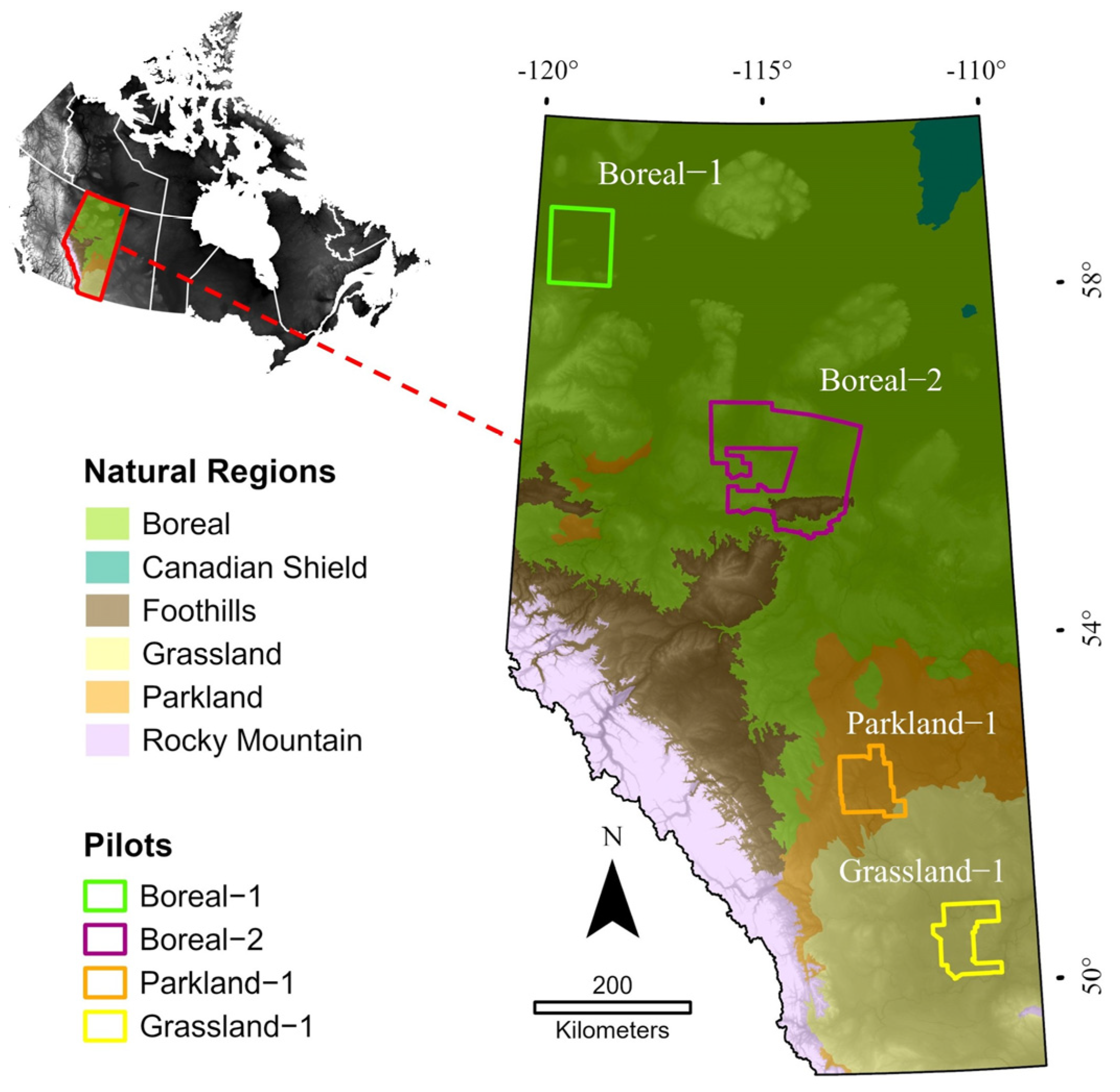
Figure 1. Four pilot area locations in relation to Canada (top left) and Alberta’s Natural Regions, adapted from [54]. The background basemap is a hillshade derived from ALOS World 3D.
Remotesensing 18 00507 g001
Figure 2. Classification detail, accuracy, and MMU standards for Alberta wetland mapping. Note that the tilled marsh form (designated in white) is not part of the GOA Wetland Classification System or pilot project requirements and was included specifically for the purposes of this study.
Remotesensing 18 00507 g002
Figure 3. Flow chart of generalized study design. Note that RS inputs, reference data, and AI models slightly differ by zone, but are fully described in Section 2.5.1, Section 2.5.2, Section 2.5.3 and Section 2.5.4.
Remotesensing 18 00507 g003
Figure 4. OA (%) results for BFZ wetland class AI model scenarios. The target OA is the blue dashed line, which is 80%. The achieved OA for each scenario is the red solid line. The best model is highlighted in green text. (a) Boreal-1. (b) Boreal-2.
Remotesensing 18 00507 g004
Figure 5. OA (%) results for BFZ wetland form AI model scenarios. The target OA is the blue dashed line, which is 70%. The achieved OA for each scenario is the red solid line. The best model is highlighted in green text. (a) Boreal-1. (b) Boreal-2.
Remotesensing 18 00507 g005
Figure 6. General wetland–upland detail confusion matrices for the best performing BFZ AI models. (a) Boreal-1. (b) Boreal-2.
Remotesensing 18 00507 g006
Figure 7. OA (%) results for PPZ wetland form AI model scenarios. The target OA is the blue dashed line, which is 70%. The achieved OA for each scenario is the red solid line. The best model is highlighted in green text. (a) Parkland-1. (b) Grassland-1.
Remotesensing 18 00507 g007
Figure 8. General wetland–upland detail confusion matrices for the best performing PPZ AI models. (a) Parkland-1. (b) Grassland-1.
Remotesensing 18 00507 g008
Figure 9. Visual comparisons of best BFZ DL and ML models. (a) Reference imagery. (b) XGBoost class detail. (c) U-Net class detail. (d) XGBoost form detail. (e) U-Net form detail.
Remotesensing 18 00507 g009
Figure 10. Visual comparisons of best PPZ DL and ML models. (a) Reference satellite imagery. (b) RF form detail. (c) XGBoost form detail. (d) U-Net form detail.
Remotesensing 18 00507 g010
Figure 11. Visual comparisons of best PPZ models for mapping rare wetland forms. (a) Reference satellite imagery. (b) Validated plot polygons, representing truth label data. (c) RF form detail. (d) XGBoost form detail. (e) U-Net form detail.
Remotesensing 18 00507 g011
Figure 12. Visual example of best performing BFZ models for mapping wetlands in burned areas. (a) Reference true colour satellite imagery. (b) Reference false colour satellite imagery (R = SWIR, G = NIR, B = Red), where pink areas correspond to a fire scar. (c) U-Net class detail. (d) XGBoost class detail.
Remotesensing 18 00507 g012
Table 1. Pilot area characteristics.
Pilot NameNatural RegionArea (km2)Description
Boreal-1Boreal7613Peatland-rich boreal landscape with mixedwood forests, diverse wetlands, and moderate forestry and energy footprint.
Boreal-2Boreal and Foothills21,214Area with mixedwood forests, diverse wetlands, and extensive forest harvesting and energy development.
Parkland-1Parkland5170Landscape with wetlands in morainal and glaciolacustrine settings, dominated by marshes and open water, interspersed with some swamp, fen, and woodland and agricultural lands.
Grassland-1Grassland5065Dry mixed grass landscape with small, hydrologically isolated marshes and ponds, largely agricultural with scattered energy and transport features.
Table 2. Sources of training and validation for AI models.
PilotModel Training DataModel Validation Data
Boreal-1 and Boreal-2Photogrammetric plotsGround and helicopter surveys
Grassland-1 and Parkland-1Photogrammetric plotsGround and drone surveys
Table 3. BFZ AI modelling scenarios. RS inputs and tests were the same for Boreal-1 and Boreal-2 pilots.
PilotScenarioAlgorithmModelling Inputs
Boreal-1 and Boreal-2B-ML-S1XGBoostXAI selected Sentinel-1 and -2 variables
B-ML-S2XGBoostXAI selected Sentinel-1 and -2 variables, AW3D30
B-ML-S3XGBoostXAI selected Sentinel-1 and -2 variables, LiDAR
B-DL-S1U-NetSelect Sentinel-1 and -2 variables, AW3D30
B-DL-S2U-NetSelect Sentinel-1 and -2 variables, LiDAR
Table 4. PPZ AI modelling scenarios. RS inputs and tests were the same for Parkland-1 and Grassland-1 pilots.
PilotScenarioAlgorithmSegmentation SourceModelling Inputs
Parkland-1 and Grassland-1P-ML-S1RFPlanetScope (2023)Optimized PlanetScope and Sentinel-2, LevelSet
P-ML-S2RFPlanetScope (2023)Optimized PlanetScope, LevelSet
P-ML-S3RFPlanetScope (2023)Optimized PlanetScope and Sentinel-2, all LiDAR
P-ML-S4RFPlanetScope (2023)Optimized PlanetScope, all LiDAR
P-ML-S5RFOrthophotographyOrthophotography, Sentinel-2, LevelSet
P-ML-S6RFOrthophotographyOrthophotography, Sentinel-2, all LiDAR
P-ML-S7XGBoostPlanetScope (2023)XAI selected satellite and LiDAR terrain variables
P-ML-S8XGBoostPlanetScope (2023)XAI selected satellite and all LiDAR variables
P-ML-S9XGBoostOrthophotographyXAI selected satellite and LiDAR terrain variables
P-ML-S10XGBoostOrthophotographyXAI selected satellite and all LiDAR variables
P-DL-S1U-Net-All PlanetScope, orthophotography, and LiDAR variables
P-DL-S2U-Net-Early season PlanetScope, and all orthophotography and LiDAR variables
P-DL-S3U-Net-PlanetScope, orthophotography, and LiDAR terrain variables
P-DL-S4U-Net-All LiDAR and orthophotography variables
P-DL-S5U-Net-PlanetScope and LiDAR terrain variables
P-DL-S6U-Net-Orthophotography and LiDAR terrain variables
Table 5. BFZ per-class and per-form F1-scores of the best performing AI models.
F1-Score F1-Score
ClassBoreal-1
(B-DL-S1)
Boreal-2
(B-ML-S3)
FormBoreal-1
(B-ML-S3)
Boreal-2
(B-ML-S3)
Water0.980.98Bare0.950.78
Aquatic vegetation-0.23
Marsh0.640.71Graminoid0.650.71
Fen0.820.68Graminoid0.260.42
Shrubby0.740.19
Wooded coniferous0.580.46
Bog0.830.83Graminoid-0.16
Shrubby-0.33
Wooded coniferous0.900.82
Swamp0.820.76Shrubby0.690.67
Wooded coniferous0.650.58
Wooded deciduous0.470.04
Wooded mixedwood-0.19
Upland0.890.96Upland0.870.96
Table 6. PPZ per-class and per-form F1-scores of the best performing AI models.
F1-Score F1-Score
ClassBoreal-1
(B-DL-S1)
Boreal-2
(B-ML-S3)
FormBoreal-1
(B-ML-S3)
Boreal-2
(B-ML-S3)
Water0.790.49Bare0.790.49
Marsh0.730.74Graminoid0.730.74
Tilled0.000.00
Fen0.00-Graminoid0.00-
Shrubby0.00-
Swamp0.18-Shrubby0.18-
Upland0.970.97Upland0.970.97
Disclaimer/Publisher’s Note: The statements, opinions and data contained in all publications are solely those of the individual author(s) and contributor(s) and not of MDPI and/or the editor(s). MDPI and/or the editor(s) disclaim responsibility for any injury to people or property resulting from any ideas, methods, instructions or products referred to in the content.