Combining Hyperspectral Preprocessing and Feature Selection with Machine Learning for Inland Water Quality Parameter Inversion

Highlights

What are the main findings?

• Constructing a high-precision inversion model for non-optically active parameters based on hyperspectral data and measured water quality parameters.
• We have found a matching preprocessing strategy and feature selection strategy for the inversion model.

What is the implication of the main finding?

• The constructed water quality parameter inversion model provides a usable solution for dynamic monitoring of water health status.
• The preprocessing and feature selection schemes that match the optimal inversion model are not fixed for different water quality parameters.

Abstract

The concentrations of carbon, nitrogen, and phosphorus in water bodies significantly influence aquatic ecological conditions. By collecting multitemporal hyperspectral data and water quality parameter data from water bodies and through systematic preprocessing of hyperspectral data combined with multimethod sensitive band selection, an optimal spectral feature subset was determined. Within a machine learning framework, multiple combined remote sensing inversion models were constructed to identify the optimal inversion model for each water quality parameter, along with corresponding preprocessing methods and sensitive bands. The results indicate that differential processing of remote sensing reflectance enhances model accuracy. Sensitive band selection effectively eliminates redundant bands, significantly improving the computational efficiency of inversion models. XGBoost demonstrated superior accuracy in constructing 240 water quality parameter inversion models because of its unique algorithmic design. However, model accuracy is not solely determined by algorithmic complexity or predictive capability but rather by the combined effect of algorithm performance and input feature quality. Verification of the inversion model’s generalization ability via an independent dataset demonstrated its capacity for generalization. These findings provide valuable insights for the reliable application of hyperspectral data in aquatic environmental remote sensing and offer support for regional water quality conservation efforts.

1. Introduction

Carbon, nitrogen and phosphorus are key elements in water environments and play significant roles in the structure and function of aquatic ecosystems. Dissolved inorganic carbon (DIC) serves as an important medium for carbon exchange between water bodies and the atmosphere and is crucial for maintaining the chemical stability of water. Ammonia nitrogen (NH₃-N) and nitrate nitrogen (NO₃⁻-N) are essential nitrogen sources for the growth of aquatic organisms and directly participate in the synthesis of proteins and nucleic acids within their bodies. Total phosphorus (TP), a limiting factor for primary productivity in water bodies, directly affects the growth rates of algae and aquatic plants. However, excessive inputs of nutrients can disrupt the ecological balance, leading to the explosive reproduction of algae and even causing ecological problems such as eutrophication [1]. Rapid and effective monitoring of their concentrations is the key to revealing the ecological evolution laws of water environments and formulating effective water environmental protection measures.

Monitoring the concentrations of carbon, nitrogen and phosphorus in water bodies via remote sensing is a feasible approach [2,3]. Currently, scholars worldwide have used remote sensing techniques to retrieve water quality parameters in various water environments, such as inland rivers and lakes [4,5], river delta areas [6], and coastal areas [7,8]. Different data sources have also been used for the remote sensing inversion of water quality parameters, including spaceborne hyperspectral and multispectral data [6,9,10], hyperspectral and multispectral sensors carried by unmanned aerial vehicles [11,12,13], and water surface remote sensing reflectance data obtained by handheld or portable hyperspectral instruments [4,14]. In terms of inversion models, empirical models, semiempirical/semianalytical models, analytical models, and machine learning models have been adopted [8,15,16]. Experience-based models, while computationally efficient, lack a foundation in physical mechanisms. This limitation results in poor temporal and spatial transferability and makes the models susceptible to variations in regional water constituent composition [8,17]. In contrast, analytical models are grounded in radiative transfer theory, offering clear physical interpretability. However, their accuracy is highly dependent on the precise acquisition of complex parameters such as inherent optical properties (IOPs), posing significant challenges for application in inland waters with complex compositions [16]. To overcome these constraints, Machine Learning (ML) methods have emerged. Leveraging their powerful capability for nonlinear mapping and potential for multi-source data fusion, ML algorithms can effectively capture the complex nonlinear relationships between spectral data and water quality parameters. This enhances model robustness and prediction accuracy in complex environments, establishing ML as a predominant approach in remote sensing inversion for water quality parameters [18]. In recent years, the scope of water quality parameters retrieved via remote sensing has expanded from optically active constituents (OACs)—such as chlorophyll-a (Chl-a), total suspended matter (TSM), coloured dissolved organic matter (CDOM), and Secchi disc depth (SDD)—to include non-optically active constituents (NOACs) like chemical oxygen demand (COD), biochemical oxygen demand (BOD), total nitrogen (TN), total phosphorus (TP), and ammonia nitrogen. Additional auxiliary indicators, such as water temperature (WT) and salinity, have also been incorporated into inversion frameworks [4,12,19]. Furthermore, several studies have begun to explore the removal of heavy metal elements in water bodies [20].

The unique hydrogeochemical settings of karst and other special inland waters—characterized by high calcium levels and high alkalinity—promote the formation of micron-sized calcium carbonate precipitates, which differentiate their optical properties from those of ordinary inland water bodies [21]. At the same time, the composition of dissolved organic matter (DOM) is complex under the dual influence of surface leaching and aquatic biological activity, leading to strong absorption in the short-wave spectral range. This distinctive optical mechanism interferes with the inversion pathways of non-optically active constituents. Consequently, algorithms based on conventional empirical relationships or standard bio-optical models encounter “spectral ambiguity” in karst regions, where different constituents can produce similar spectral signals, ultimately resulting in inversion failure. The Pingzhai Reservoir is located in the karst area of Southwest China. In recent years, population growth and increases in industrial and agricultural activities in the Pingzhai Reservoir basin have affected local water quality [22]. In some areas of Guizhou, the concentrations of some water quality parameters in karst water exceed the standard, which has become an important regional water environment problem [23]. At present, the monitoring of the water quality parameters of the Pingzhai Reservoir is based on onsite water sample collection over a fixed period, but this method requires considerable labour and time. Therefore, the plan of this study is to build a set of high-precision remote sensing inversion models of water quality parameters under the framework of machine learning on the basis of the accumulated multistage hyperspectral data and water quality parameter data of the Pingzhai Reservoir to improve the use of water quality parameter monitoring and water ecological environment protection.

However, there are still some technical challenges in the process of model building. First, the signal-to-noise ratio of the original spectral data is low, and the collected hyperspectral signals are vulnerable to multiple interference sources, resulting in high-frequency noise in the spectral curve, which interferes with the extraction of effective features [12]. Second, hyperspectral data have the problems of information redundancy and collinearity, so it is necessary to extract key spectral indicators through effective dimensionality reduction methods. In addition, the performance of machine learning algorithms largely depends on the quality and representativeness of the input features; however, the combination of the best preprocessing method and feature selection algorithm is not fixed, and its adaptability to different machine learning models is not universal [19]. Therefore, subjecting hyperspectral data to preprocessing and feature selection is essential for optimizing the model framework and identifying the optimal modelling strategy. The specific objectives of this study include (1) constructing a spectral optimization process that integrates a variety of preprocessing methods and feature selection algorithms to suppress noise interference and mine sensitive bands with clear physical significance; (2) By designing different combination schemes, a total of 240 inversion models were developed for the four water quality parameters—DIC, NH₃-N, NO₃⁻-N, and TP—to systematically evaluate model performance under varied configurations; and (3) by comparing the performance of four machine learning algorithms (BP neural network, ridge regression, random forest, XGBoost) on different feature subsets, the applicable conditions and collaborative mechanism of different method combinations are clarified. The innovation of this study lies in the establishment of a full-chain systematic optimization strategy encompassing preprocessing, feature selection, and model coupling, which changes the randomness and experiential nature of preprocessing methods and feature selection algorithms in previous studies. Furthermore, a weak spectral information mining technique based on fractional-order differential transformation has been constructed, breaking through the limitations of traditional integer-order differential transformation.

2. Materials and Methods

2.1. Overview of the Study Area

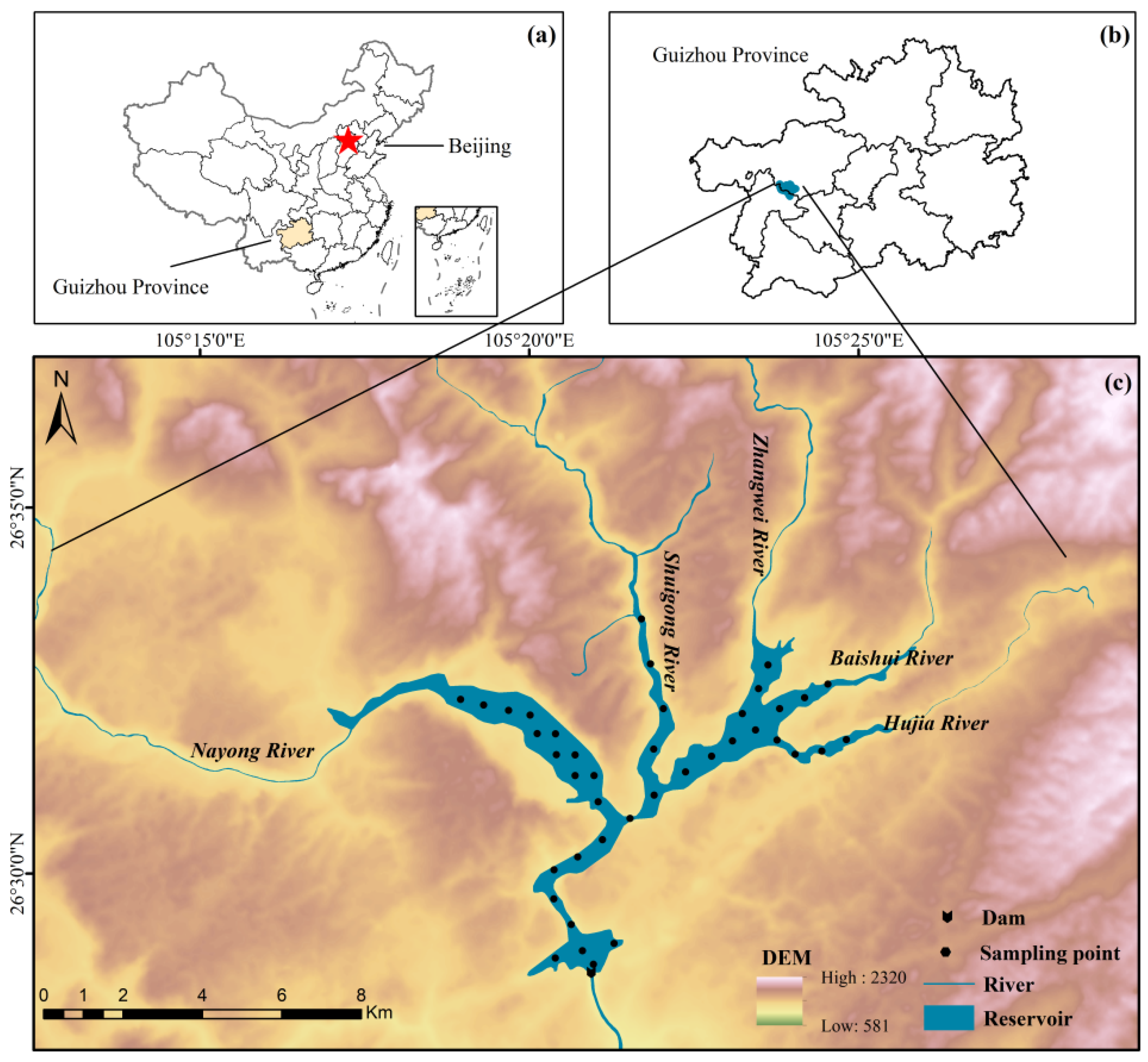
The Pingzhai Reservoir is located in the southern source of the upper reaches of the Wujiang River in the Yangtze River Basin, with geographical coordinates of 105°17′3″E–105°26′44″E, 26°29′33″N–26°35′38″N (Figure 1). The reservoir is formed by damming the Nayong River, Shuigong River, Zhangwei River, Baishui River and Hujia River. The drainage area is 833.77 km², the maximum pool level is 1331 m, and the total storage capacity is 1.089 billion m³. The study area is located in a subtropical monsoon climate area, with simultaneous rainfall and heat and four distinct seasons. The rainy season is from May to August; the normal season is from March, April, September and October; and the dry season is from November to February.

2.2. Water Sample Collection and Analysis

According to the shape and sampling accessibility of the Pingzhai Reservoir and the use of mountain shadows calculated via ArcGIS 10.8, a total of 40 surface layer (0.5 m below the water surface) water sample collection points are arranged in the Pingzhai Reservoir according to the principles of average distribution and shadow avoidance, and the locations are shown in Figure 1c. The sampling time was November 2023, April 2024, July 2024, October 2024, January 2025, and August 2025. Each sampling session synchronously collected both water samples and hyperspectral data. The hyperspectral data and water quality parameter data collected in August 2025 are used as independent datasets to verify the model effect and are not used in model training. All the collected water samples were filtered with a 0.45 μm filter membrane, put into brown sampling bottles, and then stored at 4 °C in a refrigerated environment away from light. The water sample used for the determination of NH₃-N, NO₃⁻-N and TP needs an appropriate amount of H₂SO₄ to ensure that the pH of the water sample is less than 2.0 to inhibit microbial metabolic activities through an acidic environment.

In the laboratory analysis stage, a total organic carbon analyser (TOC-VCPN, Shimadzu, Inc., Kyoto, Japan) was used to determine the DIC concentration of the water samples. The detection method used was the combustion oxidation nondispersive infrared absorption method. After preheating, the instrument was verified three times through the carbon standard solution with an accuracy of 0.001 mg/L to ensure that the coefficient of variation of the response value was ≤2%, and the final detection accuracy was controlled at 0.001 mg/L. A Cleverchem380 automatic intermittent chemical analyser (DeChem-Tech, Inc., Hamburg, Germany) was used to determine the concentrations of NH₃-N, NO₃⁻-N and TP, and the detection accuracy was 0.001 mg/L. The concentration of NH₃-N was determined via the sodium salicylate method, the NO₃⁻-N concentration was determined via the hydrazine sulfate reduction method, and the TP concentration was determined via the potassium persulfate phosphomolybdenum blue method. The pure water sample and quality control sample were inserted simultaneously during sample measurement. The measured value of the blank sample was lower than the detection limit of the method, and the relative error between the measured value of the quality control sample and the standard value was ≤5%.

2.3. Hyperspectral Data Acquisition

The hyperspectral data synchronized with the measured water quality parameters were collected under conditions of clear weather and a calm water surface. During sampling, no specific considerations were given to the growth conditions of algae and submerged macrophytes. An ASD FieldSpec 4 Standard-Res instrument (Analytical Spectral Devices, Inc., Boulder, CO, USA) was used to collect the hyperspectral data, which were obtained at 1 nm intervals. In the process of spectral measurement, to avoid interference from water specular reflection and shadows, the observation plane of the spectrometer should be at an angle of 135° with respect to the plane of the solar incidence angle and maintain an angle of 45° with respect to the normal of the water surface. The vertical distance from the spectral probe to the water surface is approximately 1 m [24]. At least 10 water surface spectra and sky diffuse radiance curves at each sampling point were collected for averaging. Considering that it is impossible to collect data due to weather conditions and that, after outliers are eliminated, 142 available spectral data points will be collected in November 2023, April, July, October 2024 and January 2025. Owing to the strong absorption of water after the 900 nm band, the signal intensity of these bands decreases, and the effective information of water is very limited. Therefore, this study uses only the band between 350 nm and 900 nm to establish an inversion model of water quality parameters. The calculation method of Li et al. [24] was used for the remote sensing reflectance of water bodies.

2.4. Hyperspectral Data Preprocessing Methods

Because the data acquisition process is easily affected by factors such as sensor characteristics, environmental noise and atmospheric interference, the original data often contain noise, baseline drift and outliers, which interfere with the accuracy and reliability of the inversion model [25,26]. The hyperspectral data preprocessing methods used in the study are introduced below.

2.4.1. Abnormal Curve Elimination and Average Value Processing

The elimination of outliers and the averaging of the hyperspectral data are carried out mainly via Viewspec Pro 6.2 software. The abnormal curves are manually recognized and eliminated according to the spectral morphological characteristics (such as the smoothness of the curve and whether there are obvious outlier jumps). All normal curves are then selected to calculate the average value, and a representative average spectral curve is finally output.

2.4.2. Scattering Correction of Hyperspectral Data

The standard normal variable (SNV) is used to correct the scattering of hyperspectral data. The core principle is to centralize and scale each individual spectral curve [16]. This processing can effectively suppress the scattering interference and baseline effect to improve the correlation between the spectrum and the target variable.

2.4.3. Hyperspectral Data Smoothing

The common smoothing method for spectral data analysis is convolution smoothing, which was proposed by Savitzky and Golay [27]. This process can reduce the high-frequency random noise introduced by the sensor dark current and environmental fluctuations [28]. When processing, the S-G method with a window size of 5 and a polynomial order of 2 is selected to smooth the remote sensing reflectivity.

2.4.4. Hyperspectral Data Differential Processing

Hyperspectral differential processing is a spectral enhancement technology based on numerical differential operations. The derivative of the reflectivity with respect to the wavelength is calculated to amplify the subtle change in the spectral curve. Differential transformation can remove the noise unrelated to water quality parameters in the spectrum by eliminating background interference, enhancing the resolution of characteristic peaks, linearization and other functions so that the effective information directly related to water quality parameters in the spectrum is more prominent.

In addition to integer-order differentiation, fractional-order differentiation has gradually become the mainstream method of hyperspectral data preprocessing [29]. The fractional differential has three main definitions: Grunwald–Letnikov (G-L), Riemann–Liouville (R-L) and Caputo, which are applicable to different fields because of their different mathematical properties. Among them, the G-L definition is based on the difference principle. Its discrete form is highly suitable for digital signal processing, image texture enhancement and hyperspectral data numerical calculation. It is a common tool for realizing fractional differential operations. In this study, the integer order differential order for hyperspectra is 1 and 2, and the fractional order differential order is 0.5 and 1.5.

As mentioned above, the hyperspectral data are first removed from outliers and processed with average values. Then, the baseline offset and background noise are eliminated via SNV, and the data are smoothed via S-G filtering to improve the signal-to-noise ratio. Finally, integer-order and fractional-order differential processing are performed to enhance the spectral characteristics and obtain the best spectral morphology.

2.5. Sensitive Band Screening Method

When preprocessed hyperspectral data are used for modelling, spectral feature extraction and sensitive band screening are usually carried out. Because not all wavebands effectively respond to water quality parameters and the inversion of water quality parameters often depends on mathematical models, too many wavebands sharply increase the dimension of the model input, leading to “dimensional disaster”. In addition, the spectral response mechanisms of different water quality parameters are different. Through the screening of sensitive bands, the band with the most significant response to the target water quality parameters was identified.

On this basis, three typical data dimensionality reduction algorithms are used to determine the effective wavelength: competitive adaptive reweighted sampling (CARS), variable importance in projection (VIP) and variable combination population analysis-iterative retaining informative variables (VCPA-IRIV). These three methods are introduced below.

2.5.1. CARS

Cars is a screening technique that combines Monte Carlo sampling (MCS) and partial least squares regression (PLSR) coefficients [14]. Through the adaptive weighted sampling mechanism, the algorithm retains the sample points with higher absolute values of the regression coefficient in the partial least squares regression model in each iteration and removes the sample points with lower weights to construct a new subset. The partial least squares regression model was then re-established on the basis of the new subset. After multiple rounds of operation, the spectral wavelength corresponding to the subset with the smallest root mean square error of cross-validation (RMSECV) was selected as the sensitive wavelength of the model input. In terms of parameter setting, 50 MCS iterations are set. In each sampling iteration, 5-fold cross-validation is used to evaluate the minimum cross-validation root mean square error of the calculation model.

2.5.2. VIP

The core idea of the variable projection importance index is to identify the most predictive sensitive band by quantifying the contribution of each independent variable to explaining the variation in the dependent variable [30]. The characteristic of this method is that it comprehensively considers the direct correlation between band and water quality parameters and the indirect role of bands in potential variables and overcomes the defect that single correlation analysis has difficulty addressing the problem of band collinearity. In practical applications, VIP > 1 is used as an important criterion to judge variables. The larger the VIP value is, the greater the comprehensive contribution of variables to the model.

2.5.3. VCPA-IRIV (Hereafter Referred to as V-I)

V-I is a high-dimensional feature selection method that combines variable clustering and iterative filtering, which can achieve the dual goals of removing redundancy and preserving information [31,32]. Specifically, the VCPA method is used to classify similar variables into the same cluster to reduce the repeated impact of collinear variables. Then, the importance of variables in the cluster is dynamically evaluated via the IRIV method, and the key variables with strong explanatory power for the target variables are retained iteratively [4]. In terms of parameter setting, the number of cross validations of the algorithm is 5, the preprocessing method is “center”, the number of runs of the exponential decline function (EDF) is set to 50, and the number of runs of binary matrix sampling (BMS) is set to 1000.

2.6. Machine Learning Algorithm

A hyperspectral remote sensing inversion model of the water quality parameters of the Pingzhai Reservoir was established via machine learning algorithms such as the BP neural network (BPNN), ridge regression (RR), random forest (RF) and eXtreme Gradient Boosting (XGBoost).

2.6.1. BPNN

The BPNN is a multilayer feedforward neural network trained on the basis of an error backpropagation algorithm. It was proposed by Rumelhart et al. [33] and is one of the most widely used neural network models at present. The core idea is to use the gradient descent method to search iteratively in the parameter space through the two processes of forward calculation and error back propagation to minimize the error. Because of their structural flexibility and modelling ability, BPNNs are widely used in complex nonlinear regression tasks such as water quality parameter inversion. Its performance largely depends on the network structure design, superparameter optimization and mechanism used to address overfitting [34].

2.6.2. RR

The RR algorithm is an improved linear regression method with an L₂ regularization term that aims to solve the problems of unstable solutions and high model variance in the processing of multicollinearity data via the ordinary least squares method [35]. RR is particularly suitable for high-dimensional data modelling, spectral analysis, image processing and other fields [36]. For example, the remote sensing retrieval of hyperspectral water quality parameters can effectively address the high correlation between hundreds of bands and provide more robust regression estimates.

2.6.3. RF

RF is an integrated learning algorithm that improves the prediction accuracy and robustness of a model by constructing multiple decision trees and performing integrated voting or averaging [37]. The algorithm combines the bagging integration idea and a random feature selection mechanism and processes high-dimensional data through the repeated return of binary data. The RF improves the prediction accuracy without increasing the computational complexity. Because it is insensitive to multicollinearity, it is widely used in hyperspectral remote sensing classification and environmental parameter inversion.

2.6.4. XGBoost

XGBoost is a machine learning technique for regression and classification problems. The gradient boosting decision tree (GBDT) framework significantly improves the training efficiency, prediction accuracy and generalization ability of the model by introducing L₁ and L₂ regularization terms, sparse data optimization, parallel computing and other mechanisms. Unlike the bagging strategy adopted by RF, XGBoost uses a boosting method to combine a series of relatively weak learners into a powerful integrated model through gradual optimization [38], so it has better prediction ability.

2.7. Model Accuracy Evaluation Method

The accuracy and stability of the inversion model were evaluated via three metrics: the root mean square error (RMSE), coefficient of determination (R²), and mean absolute error (MAE). The specific calculations followed the methodology described in Li et al. [24]. With respect to the interpretation of these metrics, a higher R² value coupled with lower RMSE and MAE values indicates greater model accuracy and improved prediction performance.

2.8. Data Processing Methods

The data processing software used was primarily MATLAB 2019b, Unscrambler X 10.4, IBM SPSS Statistics 26.0, Origin 2024, ViewSpecPro 6.2, and the Python 3.11 programming language. Specifically, Unscrambler X 10.4 was employed for hyperspectral data preprocessing. MATLAB 2019b was used to construct feature extraction models for sensitive bands. IBM SPSS Statistics 26.0 and Origin 2024 were employed for statistical analysis and data visualization. ViewSpecPro handles spectral data processing and analysis tasks, including outlier curve removal and reflectance averaging. Machine learning code development and execution were based on the scikit-learn library within the Python programming language.

3. Results

3.1. Concentration Characteristics of Water Quality Parameters

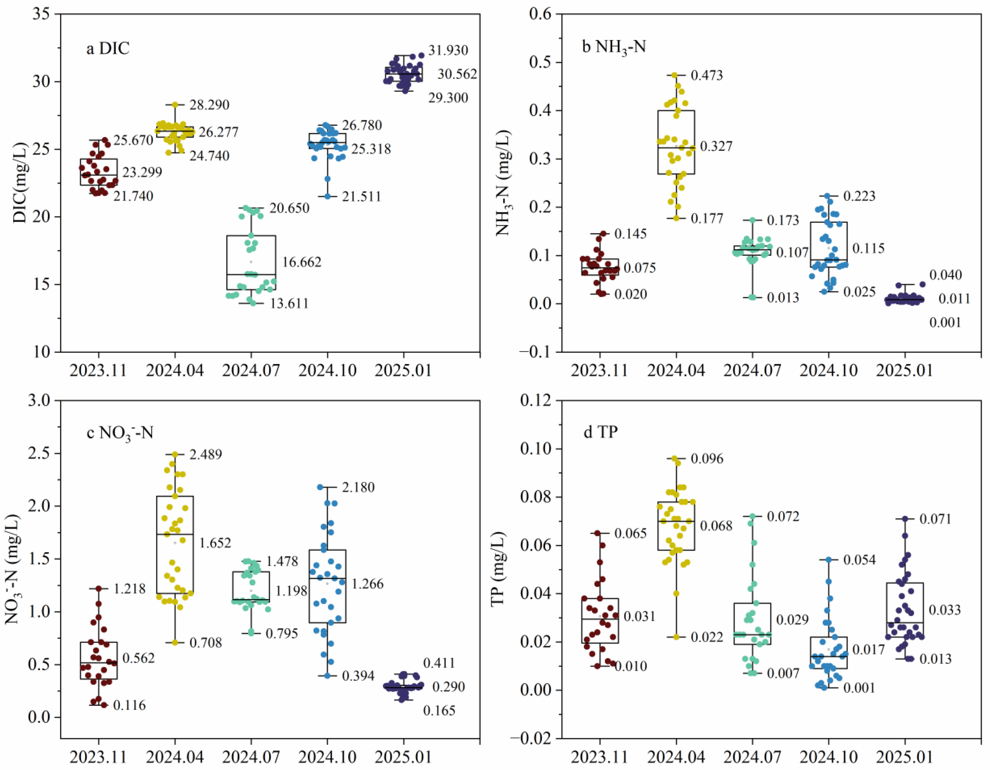
To visually illustrate the trends in various water quality parameters, box plots were generated for different sampling periods (Figure 2). The upper and lower horizontal lines of each box represent the maximum and minimum values within that dataset, respectively, whereas the central data point indicates the mean value. A longer box signifies greater data dispersion and increased variability, whereas a shorter box indicates more concentrated and stable data.

As shown in Figure 2, the DIC concentration peaked in January 2025, with an average value of 30.562 mg/L and a maximum value of 31.930 mg/L. Conversely, the lowest concentration occurred in July 2024, with an average of 16.662 mg/L and a minimum value of 13.611 mg/L. NH₃-N concentrations peaked in April 2024, with an average of 0.327 mg/L. The average values remained lower during other periods, indicating minimal concentration fluctuations. NO₃⁻-N concentrations were elevated in April and October 2024, averaging 1.652 mg/L and 1.266 mg/L, respectively, with a dispersed data distribution and significant variability. Lower averages were recorded in November 2023 (0.562 mg/L), July 2024 (1.198 mg/L), and January 2025 (0.290 mg/L), with a concurrent narrowing trend in the range of concentration extremes. The average TP concentration in April 2024 was 0.068 mg/L. Other periods, such as November 2023, July and October 2024, and January 2025, presented relatively low average values, with overall lower dispersion in concentrations across these periods.

3.2. Remote Sensing Reflectance Characteristics

3.2.1. Characteristics of Raw Remote Sensing Reflectance and Reflectance Processed via SNV + S-G

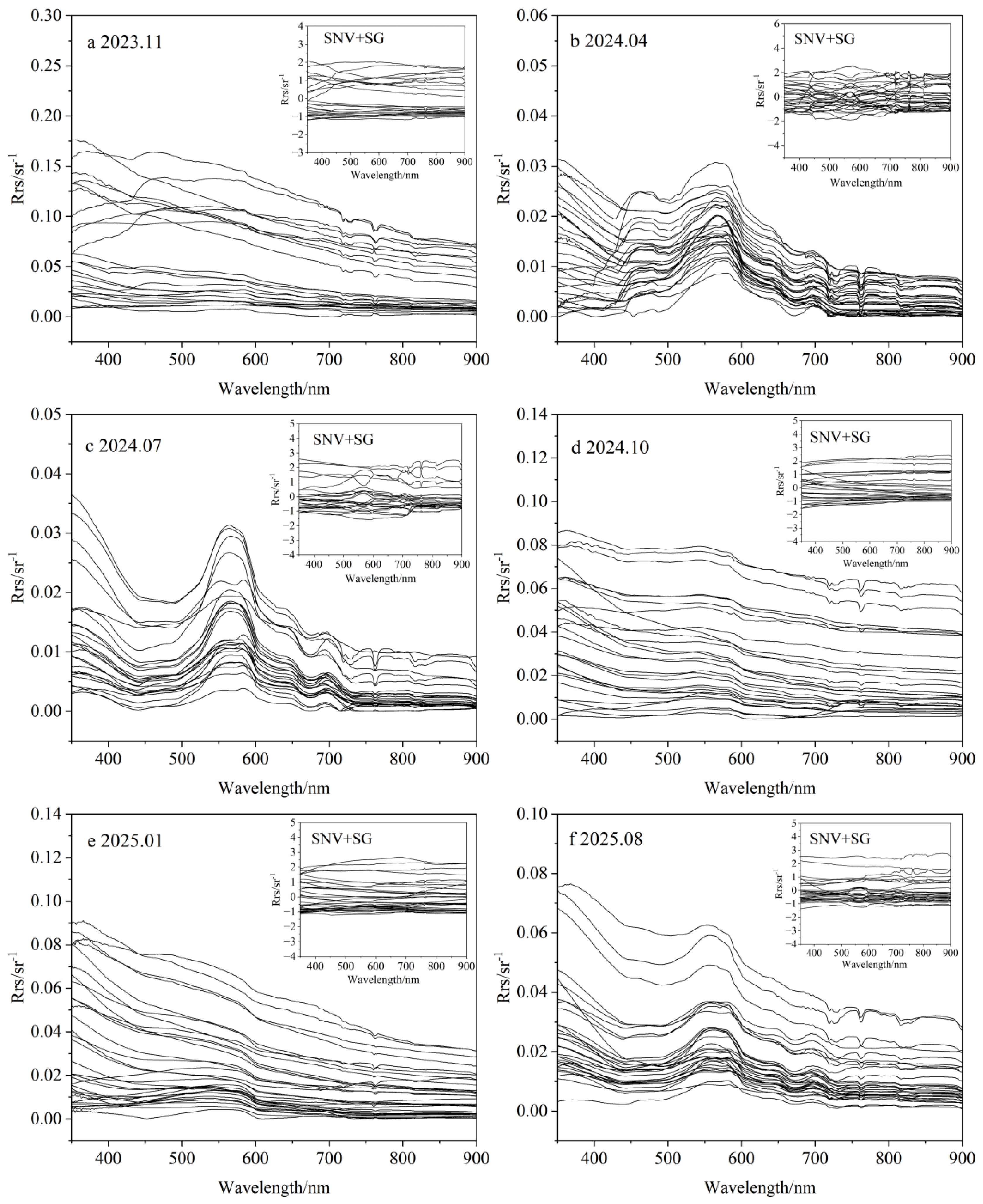
As evident from the measured hyperspectral data of the Pingzhai Reservoir collected across various months (Figure 3), the locations of high and low values of water body remote sensing reflectance remained relatively consistent across different periods. However, the intensities of the absorption and reflection peaks slightly vary. This discrepancy primarily stems from the seasonal dynamics in the concentration and composition of substances within the water body, the incident light field, and the surface state of the water.

Taking the remote sensing reflectance of the Pingzhai Reservoir in July 2024 as an example, it can be observed that the reflectance exhibits typical characteristics of inland water bodies. Within the 400–500 nm range, water reflectance is low, primarily due to the strong absorption of chlorophyll a and CDOM in the blue-violet wavelength band. A distinct reflectance peak appears near 580 nm, which is chiefly attributable to the weak absorption of chlorophyll a and carotenoids, coupled with cellular scattering. A trough or shoulder-like feature near 620 nm arises mainly from phycocyanin absorption. A chlorophyll a absorption peak appears near 670 nm, with a reflection peak emerging at approximately 690–700 nm. The reflection peak in the 690–700 nm range constitutes the most distinctive spectral feature of algal waters. In the longwave region (750–900 nm), the water reflectance decreases rapidly. The effects of SNV and S-G filtering are illustrated in the inset plots in the upper right corner of each figure. This processing mitigates baseline drift caused by water turbidity and light intensity by eliminating overall intensity variations between samples (normalizing the mean to 0 and the standard deviation to 1), thereby enabling spectral curves from different seasons or regions to be compared on a consistent scale [3].

3.2.2. Characteristics of Remote Sensing Reflectance Following Differential Processing

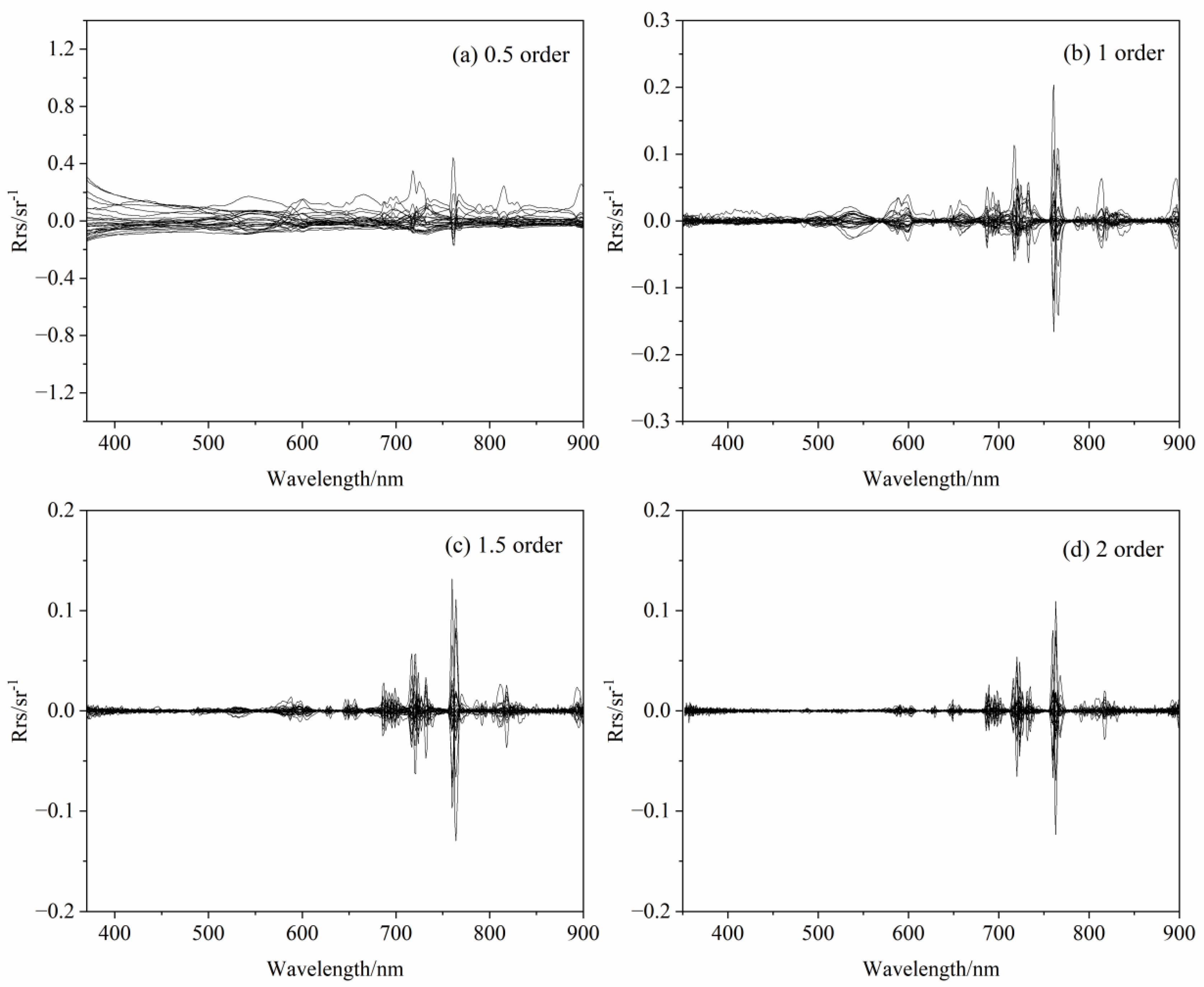
The study simultaneously employed integer-order and fractional-order differentiation methods to apply differential transformations to the original remote sensing reflectance data. The results of processing July 2024 remote sensing reflectance data are presented in Figure 4. As evident from the figure, after 0.5-order differentiation, the spectral curve appears relatively smooth while retaining much of the original spectral trend, with subtle features becoming more pronounced. One-order differentiation renders spectral variations more pronounced, accelerating the rate of reflectance change with wavelength and accentuating characteristic peaks and troughs. The 1.5-order differentiation further amplifies details, magnifying subtle variations and introducing more complex fluctuations in the curve. Two-order differentiation delves deeper into the fine spectral structure, clearly revealing high-frequency variations. Different differentiation orders strike varying balances between feature enhancement and noise control, reflecting distinct capabilities in extracting spectral information. Peaks and troughs on the spectral curve become progressively more pronounced and sharply defined with increasing differentiation order, indicating that differentiation transforms accentuated spectral curve characteristics and highlights feature intervals sensitive to water quality parameter responses [39].

3.2.3. Correlation Analysis Following Differential Processing

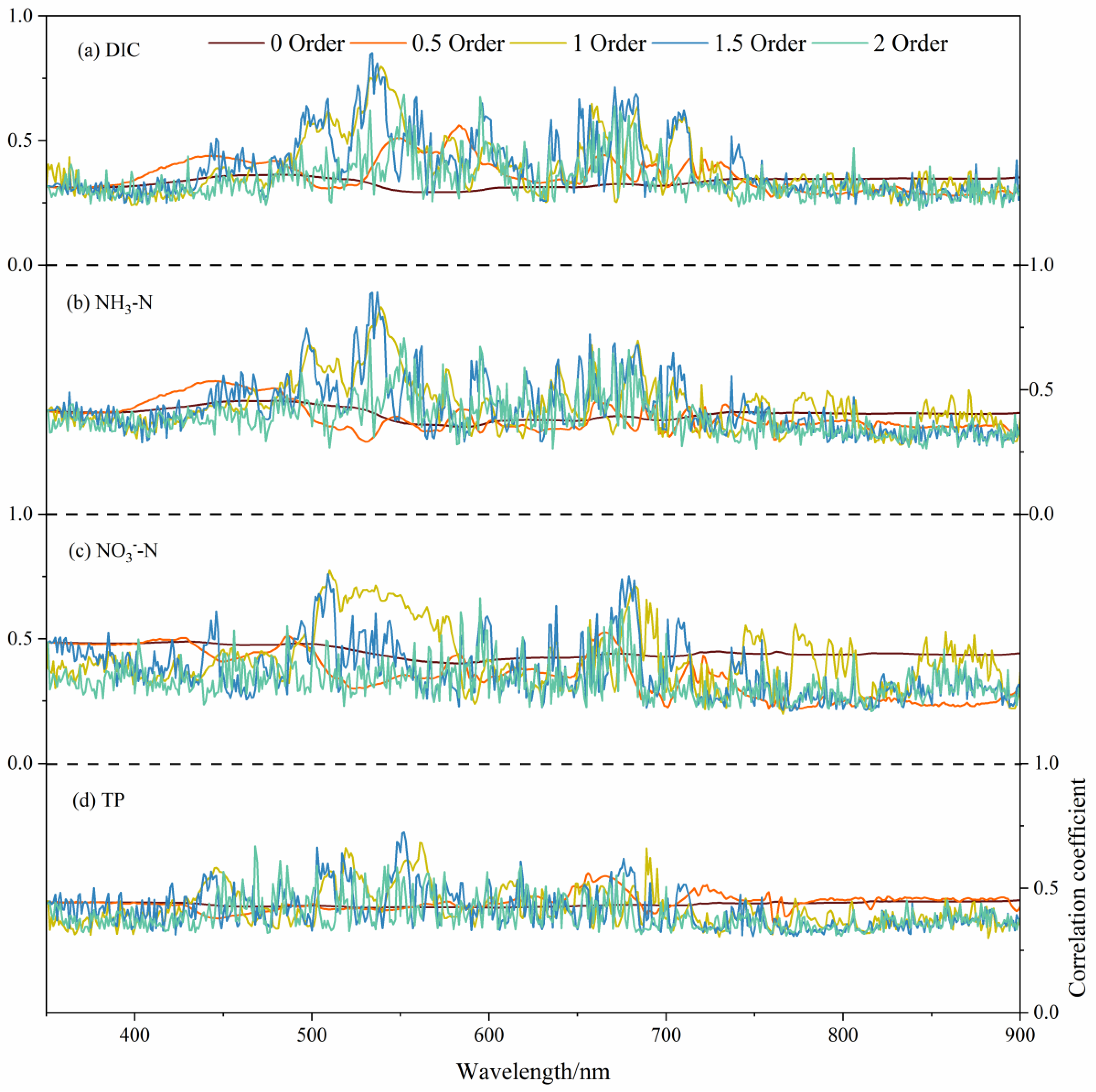
An analysis was conducted on the correlation between remote sensing reflectance processed through different differential orders and various water quality parameters, with the results presented in

Table 1. Maximum correlation coefficients for various water quality parameters following differential order processing.

Water Quality Parameters	Differential Order
	0 Order	0.5 Order	1st Order	1.5 Order	2nd Order
DIC (mg/L)	0.36	0.56	0.81	0.85	0.69
NH3-N (mg/L)	0.45	0.53	0.83	0.87	0.71
NO3−-N (mg/L)	0.55	0.58	0.77	0.76	0.71
TP (mg/L)	0.41	0.51	0.63	0.69	0.62

and Figure 5 (where the zero-order represents the original reflectance). Table 1 shows that, compared with the raw reflectance, the reflectance after differential processing is significantly more strongly correlated with the water quality parameters. Moreover, the maximum correlation coefficients are distributed across both the fractional and integer orders. These findings indicate that the four selected water quality parameters exhibit favourable response relationships with the remote sensing reflectance.

As evident from Figure 5, the correlation coefficient curve for the raw reflectance data exhibits an overall gentle slope, with most spectral bands displaying relatively low correlation values. This finding indicates that the raw spectra are significantly affected by background interference, such as water scattering and baseline drift. Following a 0.5-order transformation, the curve fluctuations intensify, indicating that low-order differentiation can preliminarily eliminate background noise to highlight strong characteristic signals. At the 1st-order transformation, the correlation coefficients for the water quality parameters begin to reach or approach peak values, with sharp and continuous peak shapes. At the 1.5-order transformation, curve fluctuations intensify further, and the high-correlation regions begin to fragment. Following 2nd-order transformation, curve oscillations become violent, with some peaks beginning to contract. This finding indicates that higher-order differentiation retains strong signals, but that weak signals become subject to noise interference, reflecting the potential for higher-order differentiation to amplify noise beyond feature enhancement, thereby obscuring valid signals [40,41]. The optimal differentiation order for different water quality parameters requires a comprehensive assessment incorporating band selection and model performance.

3.3. Sensitive Band Selection Based on CARS, VIP and V-I

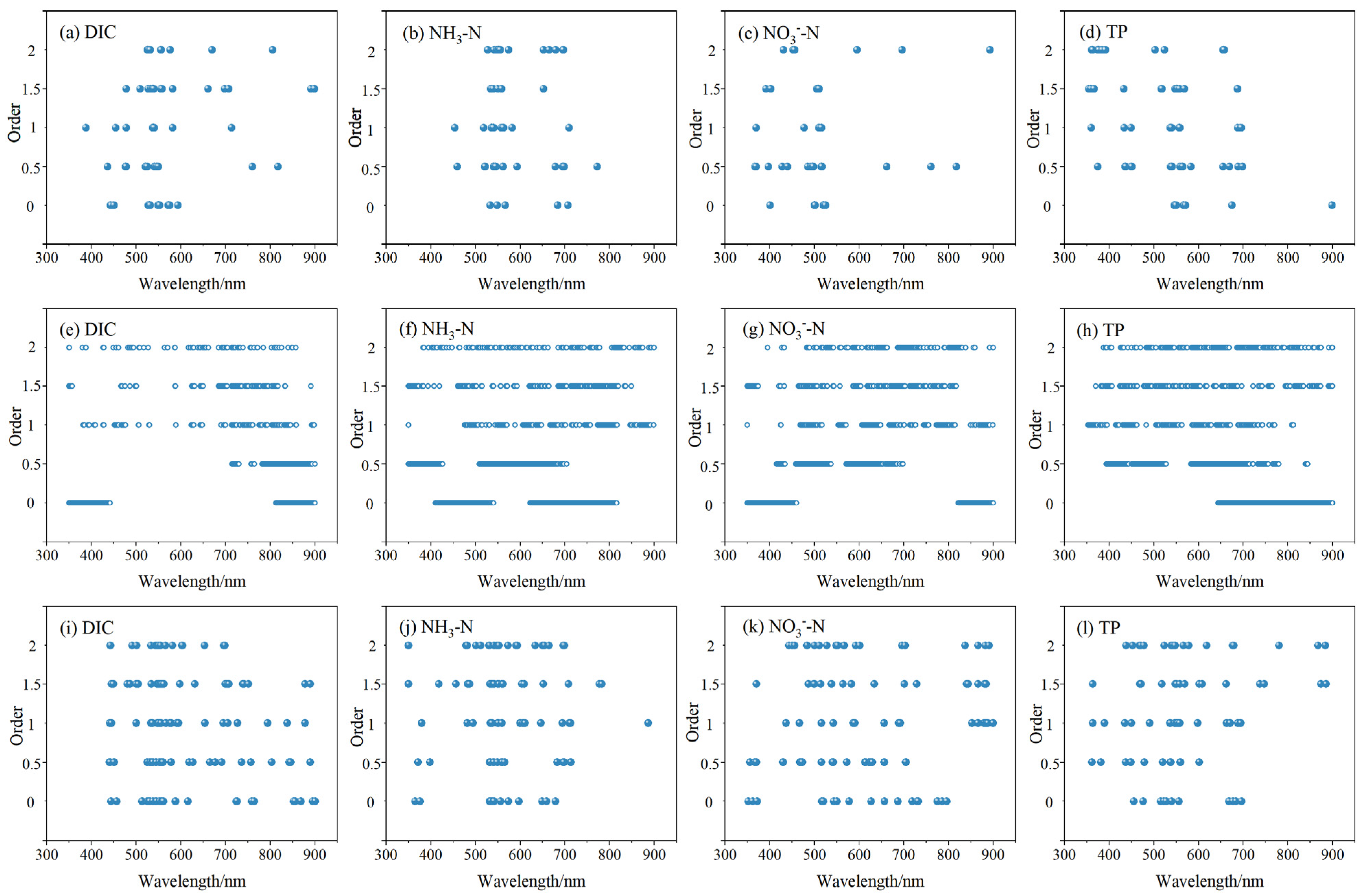
The results of the sensitive band selection are presented in

Table 2. Number of sensitive wavelength bands for CARS, VIP and V-I screening.

Order	Filter Quantity
	CARS				VIP				V-I
	DIC	NH3-N	NO3−-N	TP	DIC	NH3-N	NO3−-N	TP	DIC	NH3-N	NO3−-N	TP
0	18	5	8	9	181	326	190	257	26	14	19	12
0.5	17	18	16	18	134	261	214	304	13	17	28	12
1	10	13	6	12	125	213	217	224	40	19	17	19
1.5	18	6	8	17	107	195	185	203	26	21	18	16
2	10	15	6	14	74	142	159	217	28	29	21	20

and Figure 6. Compared with the original number of bands, the number of sensitive bands selected via CARS was significantly lower. Altering the differentiation order did not induce systematic variations in the number of bands retained by CARS, nor were discernible patterns observed between different water quality parameters and the final number of screened bands. This finding indicates that the algorithm’s screening results exhibit neither systematic bias attributable to spectral preprocessing methods (such as differentiation order) nor selective sensitivity towards specific water quality parameters.

Following VIP screening, a greater number of spectral bands were retained, which is related to the inherent mechanism of the VIP algorithm itself. Furthermore, as the differentiation order increases, the total number of retained spectral bands generally tends to decrease. As can also be observed in Figure 6, the spectral bands selected at low to medium orders predominantly display a continuous distribution, whereas with increasing differentiation order, the selected spectral bands exhibit a discontinuous distribution.

The number of bands retained through V-I method screening lies between CARS and VIP. The number of sensitive bands preserved at different differentiation orders shows no discernible pattern of variation, with the retention count for each water quality parameter remaining relatively stable. Moreover, the selected sensitive bands exhibited a broad and relatively uniform distribution range. This primarily stemmed from its unique two-stage screening mechanism, which effectively prevented excessive clustering of results near individual strong absorption peaks. Consequently, the final band subset more comprehensively and evenly reflected the combined spectral response characteristics of different components within the water body, resulting in a more extensive and uniform spatial distribution.

Although these parameters lack direct spectral absorption features in the visible-to-near-infrared region, they are tightly coupled with optically active constituents such as Chl-a, TSM, and CDOM through biogeochemical processes. For DIC, sensitive bands were identified in the green region (e.g., 509, 536, 540, 558 nm) and in the red/red-edge region (661, 707 nm). The response in the green bands likely captures the scattering signal of calcium carbonate precipitates, which are in dynamic equilibrium with DIC in karst waters. The red/red-edge bands correspond to Chl-a absorption and fluorescence, reflecting phytoplankton utilization of DIC during photosynthesis. For nitrogen species (NH₃-N, NO₃⁻-N), sensitive bands were selected in the ultraviolet-blue region (e.g., 350, 392, 456, 480 nm) and in the green region (505–511, 550, 562 nm). The UV-blue bands fall within the strong absorption range of CDOM. Since dissolved nitrogen often shares common sources with organic matter, the algorithm uses CDOM absorption as a proxy. The green bands are associated with algal pigments; as nitrogen is a key driver of algal blooms, the model indirectly infers nitrogen levels by capturing phytoplankton-induced changes in water colour. For TP, sensitive bands were identified in the red and near-infrared regions (e.g., 662, 737–747, 874, 886 nm). The red band corresponds to Chl-a absorption, indicating the contribution of biologically incorporated phosphorus in phytoplankton. The NIR bands represent typical scattering peaks of TSM. In inland waters, phosphorus is predominantly adsorbed onto suspended sediment particles. The selection of these bands confirms that the model largely relies on the adsorption correlation between total phosphorus and suspended matter.

3.4. Construction of Inversion Models Based on Machine Learning Algorithms

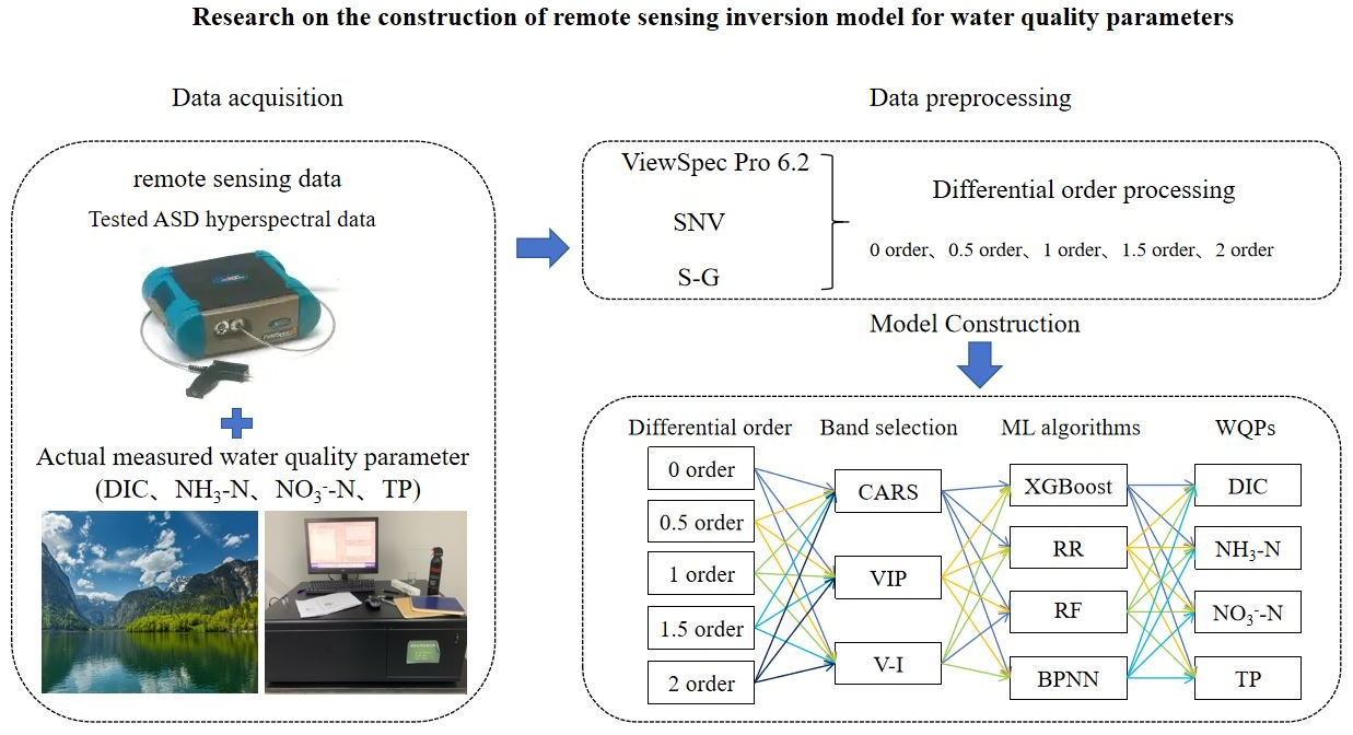
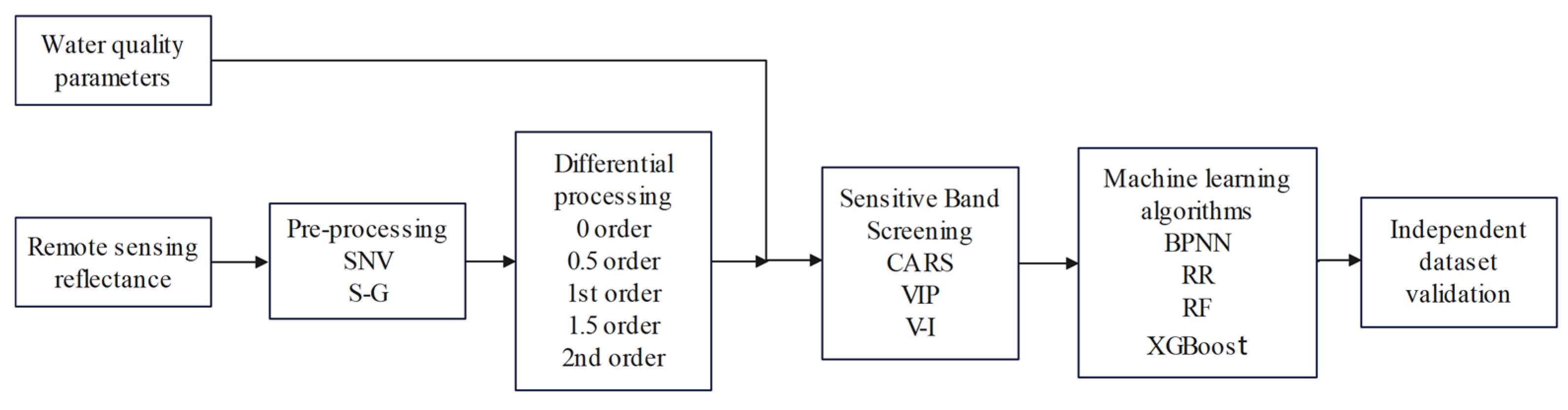
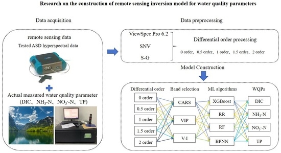
Following hyperspectral preprocessing and feature selection, four machine learning algorithms—BPNN, RF, RR, and XGBoost—were employed to establish inversion models. Specifically, the preprocessed raw remote sensing reflectance (0th order) undergoes differential transformations (0.5, 1, 1.5, 2). Subsequently, three sensitivity band selection methods are applied to each of the five reflectance datasets. Each water quality parameter yields 15 feature subsets, which are then modelled using four machine learning algorithms. This process establishes 60 distinct model combinations per water quality parameter, resulting in a total of 240 inversion models for the four water quality parameters. The overall workflow is illustrated in Figure 7.

During model training, the 142 spectral datasets were divided into training and testing sets at a 7:3 ratio. Grid search combined with fivefold cross-validation was employed to optimize the hyperparameters of each machine learning algorithm, enabling the algorithms to extract the most generalizable patterns from the data. On the basis of the determined optimal hyperparameters, the model was trained on the entire training dataset. The final model accuracy was assessed via metrics such as R², RMSE, and MAE, which were calculated on the test dataset. The primary hyperparameters ultimately set for each algorithm in the study are shown in

Table 3. Key hyperparameter settings for different machine learning algorithms.

Machine Learning Algorithms	Main Hyperparameters	Water Quality Parameters
		DIC	NH3-N	NO3−-N	TP
BPNN	hidden_layer_sizes	7	6	6	5
	learning_rate_init	0.1	0.01	0.01	0.01
	max_iter	1000	1000	1000	1000
	tol	0.0001	0.0001	0.0001	0.0001
RF	n_estimators	100	100	100	100
	max_depth	None	None	None	None
	min_samples leaf	2	5	1	1
	min_samples_split	2	2	5	2
RR	Alpha	3	6	2	3
	degree	2	2	2	2
XGBoost	n_estimators	105	100	70	135
	learning_rate	0.1	0.05	0.1	0.1
	max_depth	3	3	6	3
	min_child_weight	2	1	1	2
	gamma	0	0.5	0.2	0

.

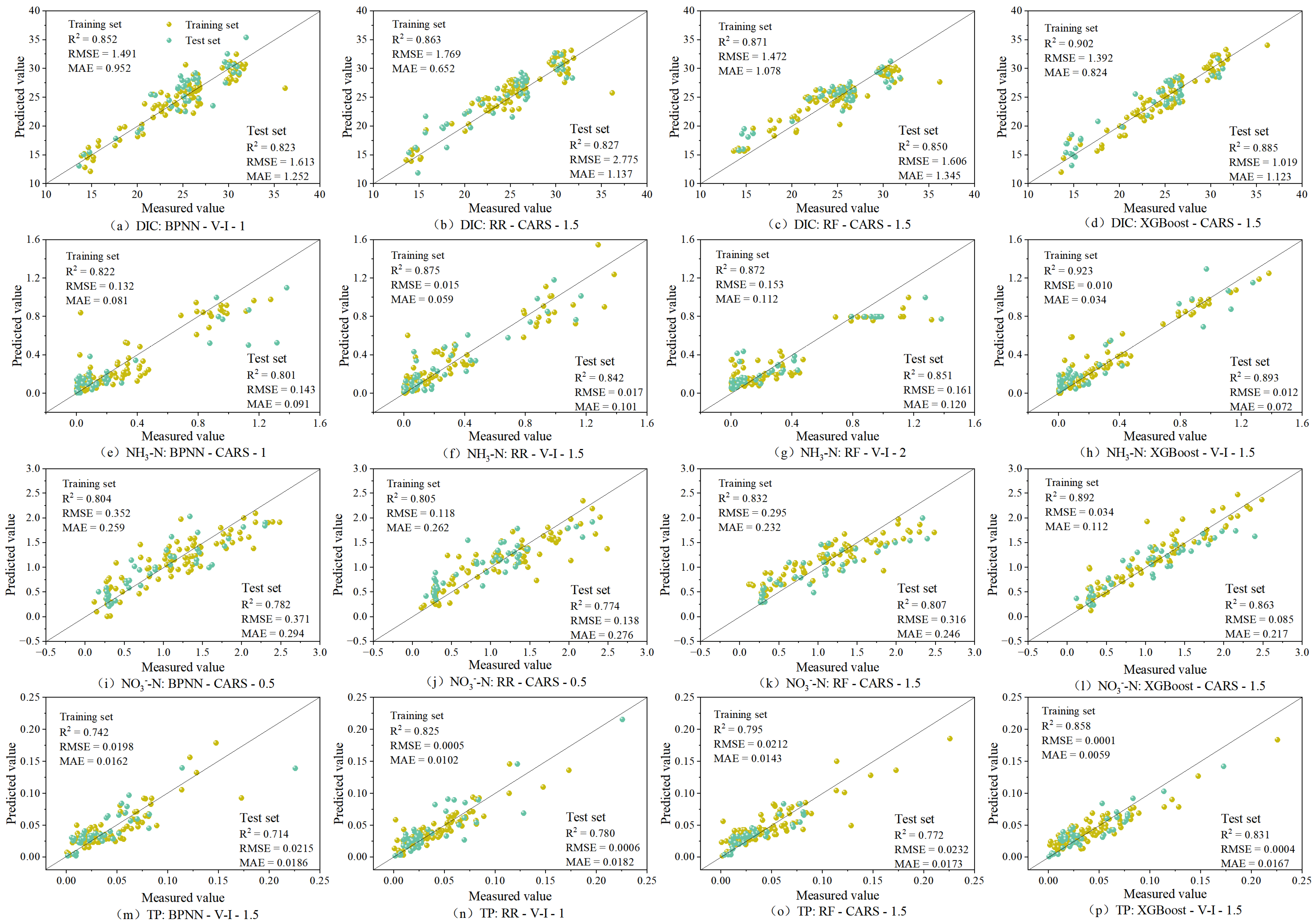
To conserve space, only the optimal inversion model for each water quality parameter under the four machine learning algorithms is presented (Figure 8). The accuracy performance of the remaining models is detailed in the Supplementary Materials. As shown in Figure 8, the optimal inversion models for each water quality parameter exhibit varying differential orders and feature band selection methods, with notable differences in accuracy among the algorithms. For the DIC inversion models (Figure 8a–d), the XGBoost-based model achieved the highest R² values in both the training and testing datasets, at 0.902 and 0.885, respectively. The R² values of the XGBoost model for the testing dataset were 0.07, 0.05, and 0.04 higher than those of the BPNN, RR, and RF models, respectively. In the NH₃-N inversion models (Figure 8e–h), the scatter plots for the BPNN, RR, and RF models showed greater dispersion than did the XGBoost model. The XGBoost model achieved the highest R² values for both the training and testing datasets, at 0.923 and 0.893, respectively. For the NO₃⁻-N inversion models (Figure 8i–l), the XGBoost model achieved the highest R² values in both the training and testing datasets, at 0.892 and 0.863, respectively. The R² values of the XGBoost model on the testing dataset were 0.081, 0.089, and 0.056 higher than those of the BPNN, RR, and RF models, respectively. Among the TP inversion models (Figure 8m–p), the XGBoost model achieved the highest R² values for both the training and testing datasets, at 0.858 and 0.831, respectively, with smaller prediction-to-observation errors across both datasets. Compared with the BPNN, RR, and RF models, the XGBoost model achieved higher R² values on the test set by 0.117, 0.051, and 0.059, respectively. Among all the water quality parameter inversion models, the XGBoost model demonstrated the highest accuracy, followed by the RF and RR models, whereas the BPNN model exhibited the lowest accuracy.

In studies on remote sensing inversion of water quality parameters conducted in various karst regions, Song et al. [42] developed an empirical model for TP concentration in Eagle Creek Reservoir (USA), achieving an R² of 0.65. Lim and Choi [43] constructed an empirical model for TN concentration in the Nakdong River (South Korea), with an R² of only about 0.4. Somvanshi et al. [44] established empirical models for TDS, COD, and BOD in the Gomti River (India), which is influenced by a concealed karst aquifer, with R² values as low as 0.53, 0.38, and 0.52, respectively. Cao et al. [45] demonstrated that a neural network model based on ground-based hyperspectral remote sensing data is suitable for retrieving non-optically active parameters such as nitrogen and phosphorus, though the R² for the two water quality parameters remained around 0.60–0.65. In contrast, the present study further improved inversion accuracy by introducing fractional-order derivative preprocessing and systematic feature selection methods. This enhancement underscores the critical role of refined feature engineering in optimizing model input structures and effectively extracting spectral signals from complex inland waters such as karst aquatic systems.

3.5. Model Validation via Independent Datasets

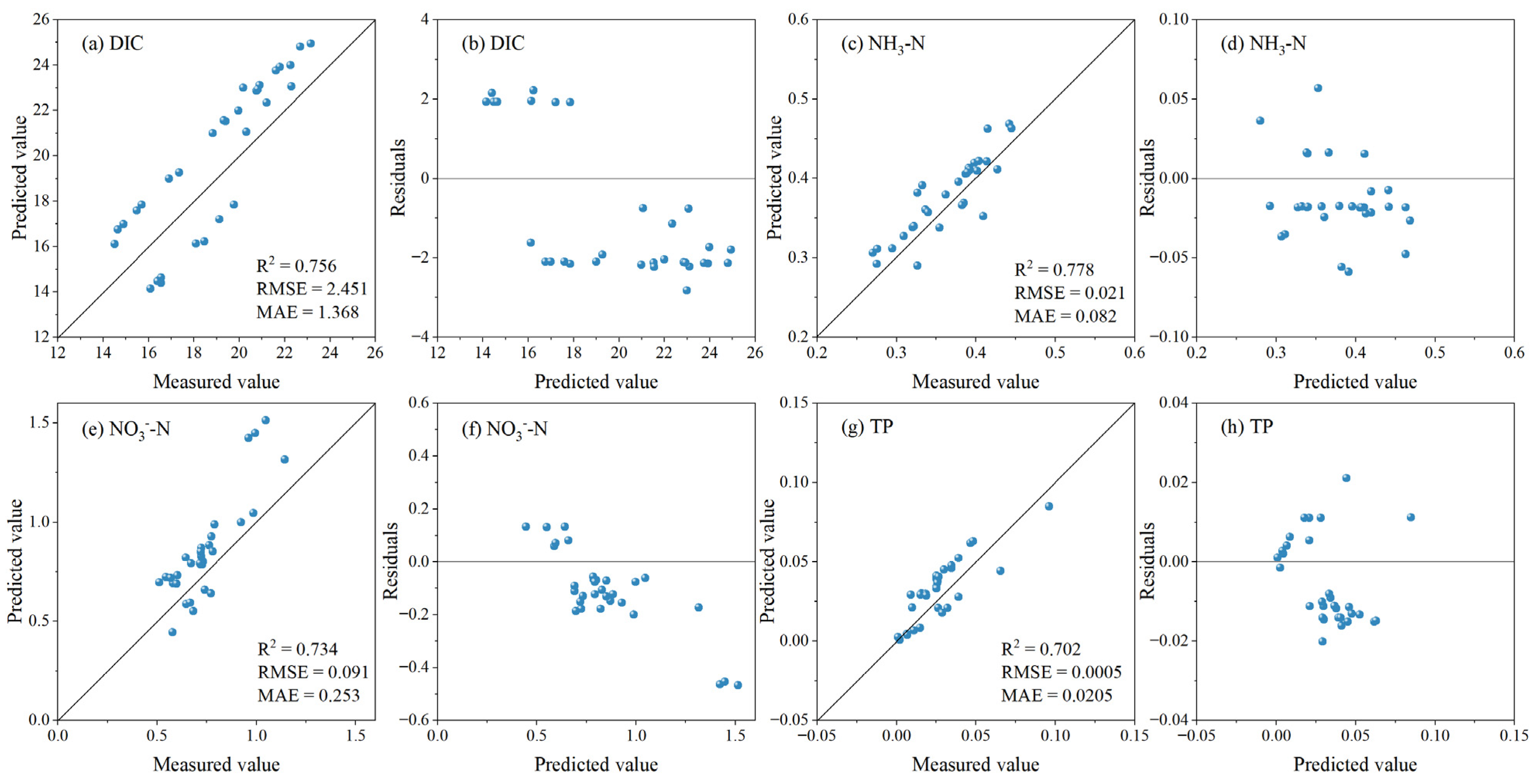
To validate the applicability of the optimal inversion model, hyperspectral data of the water surface at Pingzhai Reservoir collected in August 2025 and concentrations of various water quality parameters were used as an independent dataset to assess the model’s performance. The sampling locations and operational procedures were consistent with those used in previous studies (31 data points were obtained). For hyperspectral data acquisition, preprocessing workflows, differential order selection, and sensitive band identification, the order and bands employed by the optimal model were adopted without additional sensitive band screening for the independent dataset. The results are presented in Figure 9.

The results indicate that the model’s accuracy on the independent dataset has decreased to some extent, but the overall reduction remains within an acceptable range. The residual plots reveal that the scatter plot distribution of the predicted values versus the validation values for each water quality parameter shows no discernible trend. The residuals are randomly distributed across the entire range of the x-axis, exhibiting no obvious linear, curvilinear, or other systematic patterns. This suggests that the model adequately captures the primary patterns within the data and possesses a certain degree of generalizability.

Further analysis of the 1:1 plot comparing the predicted and validated values reveals that a portion of the predicted values for each water quality parameter lies above the 1:1 reference line. This indicates a tendency for predictions to be somewhat overestimated relative to the validated values. This phenomenon may be related to data characteristics. The validation data were collected during the August flood season, a period marked by increased precipitation in the Pingzhai Reservoir watershed and the reservoir’s water level rising to its annual peak. The abundant water produced a dilution effect on the concentrations of various substances in the water body, leading to overall lower measured values. Moreover, the average concentrations of the water quality parameters in the training set were greater than those in the validation set. During training, the model learned the data distribution characteristics of the training set, resulting in a systematic tendency to overestimate when predicting data for the high-water period. This phenomenon also reflects a common challenge faced by machine learning models in cross-period predictions. Differences in the data distributions between the training and validation sets, stemming from distinct sampling periods, caused the model to gravitate toward its familiar data domain during generalization. The study by Moradi et al. [46] demonstrated that a broader dynamic range in the training dataset enables the model to learn a more comprehensive mapping between spectral features and water quality parameters. This expands the coverage of the feature space, thereby reducing the risk of error when the model is applied to new scenarios.

Figure 8. Optimal inversion models for various water quality parameters under four machine learning algorithms (Model—Feature selection method—Differential order). ((a) DIC: BPNN - V-I - 1; (b) DIC: RR - CARS - 1.5; (c) DIC: RF - CARS - 1.5; (d) DIC:XGBoost - CARS - 1.5; (e) NH₃-N: BPNN - CARS - 1; (f) NH₃-N: RR - V-I - 1.5; (g) NH₃-N: RF - V-I - 2; (h) NH₃-N: XGBoost - V-I - 1.5; (i) NO₃⁻-N: BPNN - CARS - 0.5; (j) NO₃⁻-N: RR - CARS - 0.5; (k) NO₃⁻-N: RF - CARS - 1.5; (l) NO₃⁻-N: XGBoost - CARS - 1.5; (m) TP: BPNN - V-I - 1.5; (n) TP: RR - V-I - 1; (o) TP: RF - CARS - 1.5; (p) TP: XGBoost - V-I - 1.5).

Figure 8. Optimal inversion models for various water quality parameters under four machine learning algorithms (Model—Feature selection method—Differential order). ((a) DIC: BPNN - V-I - 1; (b) DIC: RR - CARS - 1.5; (c) DIC: RF - CARS - 1.5; (d) DIC:XGBoost - CARS - 1.5; (e) NH₃-N: BPNN - CARS - 1; (f) NH₃-N: RR - V-I - 1.5; (g) NH₃-N: RF - V-I - 2; (h) NH₃-N: XGBoost - V-I - 1.5; (i) NO₃⁻-N: BPNN - CARS - 0.5; (j) NO₃⁻-N: RR - CARS - 0.5; (k) NO₃⁻-N: RF - CARS - 1.5; (l) NO₃⁻-N: XGBoost - CARS - 1.5; (m) TP: BPNN - V-I - 1.5; (n) TP: RR - V-I - 1; (o) TP: RF - CARS - 1.5; (p) TP: XGBoost - V-I - 1.5).

Figure 9. Scatter plots of the predicted versus validated values for various water quality parameters ((a,c,e,g) show 1:1 plots; (b,d,f,h) show residual plots).

Figure 9. Scatter plots of the predicted versus validated values for various water quality parameters ((a,c,e,g) show 1:1 plots; (b,d,f,h) show residual plots).

4. Discussion

4.1. Impact of Differential Transformations of Remote Sensing Reflectance on Inversion Models

On the basis of the accuracy of the 240 constructed inversion models for various water quality parameters, compared with the original reflectance data, the majority of the models—whether they are based on integer-order or fractional-order differentiation—demonstrated improved accuracy (see Supplementary Tables S1–S4). This finding indicates that differential processing effectively enhances spectral information and improves model inversion performance. Notably, compared with integer-order differentiation, fractional-order differentiation can more precisely uncover correlations between spectral data and water quality parameters because of its continuous-order characteristics, achieving a balance between highlighting feature information and suppressing interference [12,47].

Table 4. Band selection methods and differential order for optimal inversion model matching of water quality parameters.

Machine Learning Algorithms	Water Quality Parameters
	DIC	NH3-N	NO3−-N	TP
BPNN	V-I—1	CARS—1	CARS—0.5	V-I—1.5
RR	CARS—1.5	V-I—1.5	CARS—0.5	V-I—1
RF	CARS—1.5	V-I—2	CARS—1.5	CARS—1.5
XGBoost	CARS—1.5	V-I—1.5	CARS—1.5	V-I—1.5

presents the optimal differentiation orders for each water quality parameter inversion model. The table reveals that at least two differentiation orders are optimal for each parameter, with fractional orders predominating. Except for NO₃⁻-N, which exclusively exhibits fractional orders (0.5th and 1.5th), all the other parameters incorporate both fractional and integer orders. This further indicates that in water quality parameter inversion studies, there is no fixed order for the differential processing of hyperspectral data, nor are optimal combinations universally applicable. This variability stems from differences in spectral response mechanisms among water quality parameters and variations in model-data adaptability. In specific research contexts, combinations and optimal selections must be tailored on the basis of the characteristics of the data and models.

Although modelling using differentiated remote sensing reflectance yields improved accuracy, this is not always the case. During the study, instances were observed where models based on differentiated reflectance performed worse than those built using raw reflectance. Among the 240 different combinations of inversion models constructed, the accuracies of the differentiated models were lower for 6 cases than for the raw reflectance models (

Table 5. Statistics of the cases where the inversion model after differential transformation yields lower accuracy than the original reflectance model.

Water Quality Parameters	Models (Machine Learning Algorithms—Feature Selection Methods—Differential Order)
DIC	BPNN—VIP—0.5 (R2 = 0.564); BPNN—V-I—2 (R2 = 0.730)
NO3−-N	XGBoost—V-I—0.5 (R2 = 0.683)
TP	BPNN—V-I—0.5 (R2 = 0.586); RR—VIP—2 (R2 = 0.515); XGBoost—CARS—2 (R2 = 0.551)

). However, the overall probability of this occurrence remains low, and the role and effectiveness of differential transformation in enhancing model accuracy are still evident. Furthermore, higher differential orders do not necessarily lead to greater improvements in model accuracy. Among the differential orders matched to the optimal inversion models for each water quality parameter (Table 4), 2nd-order differentiation appeared only once. Conversely, among the six models with reduced accuracy after differentiation (Table 5), second-order differentiation appeared three times. This occurs because excessively high orders may overly amplify high-frequency noise, obscuring valid signals while simultaneously oversmoothing spectral curves and causing the loss of detailed information related to water quality parameters [48].

4.2. Effect of Band Selection on Inversion Models

To compare how different sensitive band selection methods affect model performance, the optimal models for each water quality parameter were statistically identified under various sensitive band selection approaches. The models that achieved the highest accuracy were all built via the XGBoost algorithm, and the results are presented in

Table 6. Feature band selection methods and number of bands for the optimal inversion models of various water quality parameters.

	Selection Methods	Numbers	R2	RMSE	MAE		Selection Methods	Numbers	R2	RMSE	MAE
	CARS	18	0.885	1.019	1.123		CARS	16	0.872	0.015	0.085
DIC	VIP	74	0.816	2.792	1.901	NH3-N	VIP	213	0.863	0.012	0.084
	V-I	26	0.832	1.960	1.165		V-I	21	0.893	0.012	0.072
	CARS	8	0.863	0.085	0.217		CARS	17	0.802	0.0005	0.0172
NO3−-N	VIP	185	0.813	0.082	0.243	TP	VIP	203	0.763	0.0005	0.0176
	V-I	17	0.832	0.090	0.248		V-I	16	0.831	0.0004	0.0167

.

The model accuracy based on the VIP-selected sensitive bands was the lowest, and the VIP selection process retained the highest number of sensitive bands. This suggests that the selected bands may have retained redundant information unrelated to water quality parameters. This phenomenon is related to the mechanism of the VIP algorithm, which tends to retain more collinear bands with significant contributions. Consequently, adjacent bands may exceed the VIP threshold and be retained. Furthermore, inland water bodies exhibit complex optical compositions, with distinct sensitive bands corresponding to different substances. The VIP simultaneously retains the spectral intervals characterizing these diverse components, resulting in multiband screening outcomes.

The V-I algorithm retains a moderate number of bands while achieving high model accuracy. By employing a global search strategy that mimics natural selection during the VCPA phase, it avoids premature convergence to local optima. This enables the discovery of potentially valuable band combinations across diverse regions of the entire spectral range. Second, during the IRIV stage, the algorithm evaluates the contribution of each variable and its combinations through multiple iterations. Its elimination criteria do not rely solely on the strength of the linear correlation with the target parameters [49,50]. This implies that the sensitive bands retained by the V-I screening method simultaneously include both strong and weak information variables. When modelling spectral information, machine learning algorithms can capture nonlinear relationships between water quality parameters and hyperspectral data. CARS is a feature selection method based on evolutionary competition, aiming to find the most predictive subset of bands. Its search strategy is to quickly converge towards local optima, forcibly eliminating bands with weak competitiveness, resulting in the selection results tending to cluster within the core spectral feature range. Compared with those constructed with VIP-screened bands, models built with CARS-selected bands demonstrate superior accuracy.

4.3. Comparison and Analysis of the Inversion Model Results

Among the 240 inversion models constructed for various water quality parameters, those with the highest accuracy were all based on the XGBoost algorithm, demonstrating its superior model performance. The advantage of XGBoost lies in its algorithmic design adaptability to high-dimensional nonlinear relationships. By iteratively optimizing decision tree ensembles through a gradient boosting framework, it effectively mitigates overfitting risks during training through the introduction of L₁/L₂ regularization terms. Although RF is also an ensemble algorithm, its bagging-based construction strategy reduces variance by building numerous unrelated decision trees. Its default uniform voting mechanism and relatively weaker fine-tuning capabilities typically result in performance that is slightly inferior to that of XGBoost [39].

As a linear model, the inherent linear assumption of RR limits its ability to capture complex nonlinear relationships [35]. The performance of the BPNN relies on many high-quality training samples, meticulous hyperparameter tuning, and effective regularization techniques. In applications such as hyperspectral inversion, which often face scenarios characterized by a “small sample size and high dimensionality,” the network is prone to becoming stuck in local minima or overfitting [51]. There is no universally fixed optimal configuration for hyperparameters across algorithms. Their settings depend on the specific data structure and task characteristics. Different datasets exhibit significant variations in distribution, scale, noise levels, and feature dimensions, whereas different learning tasks (e.g., regression, classification, clustering) impose distinct requirements on a model’s inductive preferences. Therefore, hyperparameter optimization is fundamentally a data- and task-conditional optimization problem tailored to specific application scenarios. To enhance model generalizability and performance, this study employs scientific parameter tuning strategies such as grid search rather than relying on empirical presets.

Although the optimal inversion models for each water quality parameter were all constructed on the basis of the XGBoost algorithm, their corresponding optimal spectral preprocessing strategies and sensitive band selection methods differed. This finding indicates that the inversion accuracy of machine learning models is not solely determined by the complexity or predictive capability of the algorithm itself but rather results from the combined effects of algorithm performance and the quality of the input features. Given that the association mechanisms between different water quality parameters and spectral responses, along with their sensitive band ranges, inherently vary, their optimal preprocessing schemes must necessarily differ. This underscores the importance of integrating machine learning predictive capabilities with the spectral mechanisms of land cover features in hyperspectral inversion modelling for water quality parameters.

4.4. Uncertainty Analysis of the Inversion Results

The construction of inversion models integrates optical measurements, data preprocessing, feature selection, and machine learning modelling, with each stage introducing varying degrees of error and uncertainty. Specifically, the optical properties and biogeochemical behaviours of individual water quality parameters are core factors influencing inversion uncertainty. Different parameters result in distinct optical activities and spectral response mechanisms in water. For example, NH₃-N, NO₃⁻-N, and DIC lack direct optical absorption signatures in the visible-near-infrared (VIS-NIR) band. The influence of physicochemical conditions and biological activity in aquatic environments poses challenges for the performance of inversion models [52,53]. TPs typically exhibit the highest inversion uncertainty, as they not only lack direct spectral signatures but also exist in diverse forms (dissolved state and particle-adsorbed state). Its relationship with optical parameters is more indirect and susceptible to confounding interference from suspended particulate matter composition and algal abundance [54,55].

Hyperspectral data preprocessing and feature selection collectively constitute another significant source of uncertainty. Although methods such as S-G smoothing, SNV, and differential processing are widely employed to eliminate noise and enhance spectral features, these preprocessing techniques themselves alter the distribution and structure of the original spectra. For example, while differential processing enhances absorption troughs and reflectance peaks, it inevitably amplifies high-frequency noise (which is more pronounced at higher orders). Moreover, different differential orders yield varying information enhancement effects across sensitive spectral bands. If preprocessing methods mismatch the spectral response characteristics of target parameters, they may introduce additional errors [56]. Given the theoretical challenges of fully decoupling errors, we employed a controlled variable analysis (CVA) approach to quantify the contribution of each factor (order of differentiation, feature selection) to the variability in model performance. The range of RMSE fluctuation (RMSEmax − RMSEmin) induced by altering one factor while holding others constant was used as a metric to assess its contribution to overall uncertainty. For the error analysis of DIC, we used the best-performing model (XGBoost -CARS-1.5) as the baseline and first evaluated the influence of preprocessing (order of differentiation). While keeping the feature selection method (CARS) and the algorithm (XGBoost) fixed, results from five derivative orders (0, 0.5, 1, 1.5, 2) were compared. The RMSE varied from 1.019 to 2.451 mg/L, yielding a fluctuation range of 1.432 mg/L. Next, the impact of feature selection was assessed by fixing the preprocessing (1.5-order derivative) and the algorithm (XGBoost) and comparing three screening methods (CARS, VIP, and V-I). The RMSE changed between 1.019 and 2.207 mg/L, corresponding to a fluctuation range of 1.188 mg/L. A similar analysis was performed for NH₃-N, where the RMSE fluctuation range caused by preprocessing (order of differentiation) was 0.045 mg/L, while that caused by feature selection was 0.003 mg/L. For NO₃⁻-N, the corresponding ranges were 0.088 mg/L (preprocessing) and 0.021 mg/L (feature selection). For TP, the ranges were 0.0007 mg/L (preprocessing) and 0.0001 mg/L (feature selection). Based on the magnitude of these fluctuations, preprocessing contributed more substantially to the total error than feature selection. This quantitative comparison indicates that spectral preprocessing—in particular, the choice of fractional order derivative—is the dominant source of uncertainty. An inappropriate derivative order can lead to a marked increase in error. In contrast, once the data are properly preprocessed, the choice of feature-screening method introduces relatively minor additional variability.

In summary, the uncertainty in the hyperspectral inversion of inland water quality parameters is a complex outcome resulting from the combined effects of the parameters’ intrinsic optical behaviour, environmental dependencies, preprocessing strategies, feature selection algorithms, and model architecture. While such uncertainty is difficult to eliminate completely in remote sensing inversion, it can be effectively reduced and controlled through multifaceted optimization measures within existing methodological frameworks [57]. By meticulously refining spectral preprocessing workflows, adopting more stable feature selection algorithms, incorporating advanced machine learning frameworks, and implementing rigorous quality control processes, error propagation can be suppressed, and model robustness can be enhanced. Additionally, seasonal variations influence the accuracy of water quality inversion models through complex optical and hydrological mechanisms. Hydrological seasonality leads to distinct data distributions across seasons. When a single model trained on mixed data is applied to a specific seasonal period, it may thereby induce systematic bias. Therefore, future research should prioritize the accumulation of extensive long-term monitoring datasets to develop season-specific models.

5. Conclusions

On the basis of multiperiod hyperspectral data from the Pingzhai Reservoir and DIC, NH₃-N, NO₃⁻-N, and TP data, this study employed a systematic hyperspectral preprocessing workflow and sensitive band selection to determine the optimal feature subset for model inputs. Subsequently, remote sensing inversion models for each water quality parameter were constructed via machine learning algorithms and validated.

The research findings indicate that the correlation between reflectance after differential processing and water quality parameters has significantly improved, with both fractional and integer orders demonstrating this trend. The V-I-based sensitive band selection method can eliminate many redundant bands, which is crucial for enhancing the accuracy of inversion models and improving computational efficiency. XGBoost, with its unique algorithm design—iteratively optimizing decision tree ensembles through a gradient boosting framework while incorporating L₁/L₂ regularization terms during training—achieved the highest accuracy in the inversion models constructed for each water quality parameter.

The generalizability of the inversion model was validated via an independent dataset. The results indicate that the model’s accuracy on the independent dataset showed a certain degree of reduction, but the overall decrease remained within an acceptable range. This is attributed to the strong fluidity of water bodies, where water quality parameters themselves undergo continuous dynamic changes. Additionally, the temporal gap between the validation data and the modelling data led to discrepancies between the data distribution used for model training and the actual data distribution. This also highlights the inherent uncertainty in both the construction of the inversion model and the inversion results. Current data-driven models rely primarily on pattern learning from data distributions with limited temporal periods and spatial ranges. Consequently, they exhibit a limited ability to handle water quality states that are not fully covered or respond to extreme hydrological events. Future research should incorporate more temporal samples and conduct cross-scenario validation to further optimize model performance and generalizability.

References

1. Conley, D.J.; Paerl, H.W.; Howarth, R.W.; Boesch, D.F.; Seitzinger, S.P.; Havens, K.E.; Lancelot, C.; Likens, G.E. Controlling eutrophication: Nitrogen and phosphorus. Science 2009, 323, 1014–1015. [Google Scholar] [CrossRef] [PubMed]
2. Adjovu, G.E.; Stephen, H.; James, D.; Ahmad, S. Overview of the application of remote sensing in effective monitoring of water quality parameters. Remote Sens. 2023, 15, 1938. [Google Scholar] [CrossRef]
3. Wang, X.; Yang, W. Water quality monitoring and evaluation using remote sensing techniques in China: A systematic review. Ecosyst. Health Sustain. 2019, 5, 47–56. [Google Scholar] [CrossRef]
4. Hou, Y.; Zhang, A.; Lv, R.; Zhao, S.; Ma, J.; Zhang, H.; Li, Z. A study on water quality parameters estimation for urban rivers based on ground hyperspectral remote sensing technology. Environ. Sci. Pollut. Res. 2022, 29, 63640–63654. [Google Scholar] [CrossRef]
5. Qi, C.; Huang, S.; Wang, X. Monitoring water quality parameters of Taihu Lake based on remote sensing images and LSTM-RNN. IEEE Access 2020, 8, 188068–188081. [Google Scholar] [CrossRef]
6. Cao, Q.; Yu, G.; Qiao, Z. Application and recent progress of inland water monitoring using remote sensing techniques. Environ. Monit. Assess. 2023, 195, 125. [Google Scholar] [CrossRef]
7. Ren, J.; Cui, J.; Dong, W.; Xu, M.; Liu, S.; Zhang, J. Remote sensing inversion of typical offshore water quality parameter concentration based on improved SVR algorithm. Remote Sens. 2023, 15, 2104. [Google Scholar] [CrossRef]
8. Pan, C.; Luo, Z.; Wei, Z.; Wang, L.; Wang, M.; Peng, Y. Remote Sensing Inversion Technology for the Evaluation of Coastal Water Eutrophication with the Pressure-State-Response Framework. J. Clean. Prod. 2025, 514, 145771. [Google Scholar] [CrossRef]
9. Liang, Y.; Yin, F.; Liu, L.; Zhang, Y.; Ashraf, T. Inversion and monitoring of the TP concentration in Taihu Lake using the landsat-8 and sentinel-2 images. Remote Sens. 2022, 14, 6284. [Google Scholar] [CrossRef]
10. Ogashawara, I.; Moreno-Madriñán, M.J. Improving inland water quality monitoring through remote sensing techniques. ISPRS Int. J. Geo-Inf. 2014, 3, 1234–1255. [Google Scholar] [CrossRef]
11. Chen, B.; Mu, X.; Chen, P.; Wang, B.; Choi, J.; Park, H.; Yang, H. Machine learning-based inversion of water quality parameters in typical reach of the urban river by UAV multispectral data. Ecol. Indic. 2021, 133, 108434. [Google Scholar] [CrossRef]
12. Wang, M.; Zhou, C.; Shi, J.; Lin, F.; Li, Y.; Hu, Y.; Zhang, X. Inversion of Water Quality Parameters from UAV Hyperspectral Data Based on Intelligent Algorithm Optimized Backpropagation Neural Networks of a Small Rural River. Remote Sens. 2025, 17, 119. [Google Scholar] [CrossRef]
13. Olmanson, L.G.; Brezonik, P.L.; Bauer, M.E. Airborne hyperspectral remote sensing to assess spatial distribution of water quality characteristics in large rivers: The Mississippi River and its tributaries in Minnesota. Remote Sens. Environ. 2013, 130, 254–265. [Google Scholar] [CrossRef]
14. Zhao, H.; Song, X.; Yang, G.; Li, Z.; Zhang, D.; Feng, H. Monitoring of nitrogen and grain protein content in winter wheat based on Sentinel-2A data. Remote Sens. 2019, 11, 1724. [Google Scholar] [CrossRef]
15. Vaughn, N.R.; König, M.; Hondula, K.L.; Harrison, D.E.; Asner, G.P. Rapid Water Quality Map from Imaging Spectroscopy with a Superpixel Approach to Bio-Optical Inversion. Remote Sens. 2024, 16, 4344. [Google Scholar] [CrossRef]
16. Barnes, B.B.; Garcia, R.; Hu, C.; Lee, Z. Multi-band spectral matching inversion algorithm to derive water column properties in optically shallow waters: An optimization of parameterization. Remote Sens. Environ. 2018, 204, 424–438. [Google Scholar] [CrossRef]
17. Sun, Y.; Wang, D.; Li, L.; Ning, R.; Yu, S.; Gao, N. Application of remote sensing technology in water quality monitoring: From traditional approaches to artificial intelligence. Water Res. 2024, 267, 122546. [Google Scholar] [CrossRef]
18. Pang, Z.; Zhou, Z.; Fu, J.E.; Jiang, W.; Qin, X.; Sun, M. Deep learning-based remote sensing retrieval of inland water quality: A review. J. Hydrol.-Reg. Stud. 2025, 61, 102759. [Google Scholar] [CrossRef]
19. Cao, X.; Zhang, J.; Meng, H.; Lai, Y.; Xu, M. Remote sensing inversion of water quality parameters in the Yellow River Delta. Ecol. Indic. 2023, 155, 110914. [Google Scholar] [CrossRef]
20. Xu, X.; Pan, J.; Zhang, H.; Lin, H. Progress in Remote Sensing of Heavy Metals in Water. Remote Sens. 2024, 16, 3888. [Google Scholar] [CrossRef]
21. Hartmann, A.; Goldscheider, N.; Wagener, T.; Lange, J.; Weiler, M. Karst water resources in a changing world: Review of hydrological modeling approaches. Rev. Geophys. 2014, 52, 218–242. [Google Scholar] [CrossRef]
22. Kong, J.; Zhou, Z.; Xie, R.; Chen, Z.; Li, R.; Li, L.; Cao, W. Anthropogenic exogenous nitric and sulfuric acids in karst plateau reservoirs and their impact on carbon sinks. J. Hydrol. 2025, 660, 133394. [Google Scholar] [CrossRef]
23. Fang, S.W.; Li, Q.; Wang, R.F. Discussion on the method of searching for safe drinking water in high-sulfate areas of Guizhou Provinces. Carsologica Sin. 2019, 38, 388–393. [Google Scholar]
24. Li, Y.; Zhou, Z.; Kong, J.; Wen, C.; Li, S.; Zhang, Y.; Wang, C. Monitoring Chlorophyll-a concentration in karst plateau lakes using Sentinel 2 imagery from a case study of Pingzhai reservoir in Guizhou, China. Eur. J. Remote Sens. 2022, 55, 1–19. [Google Scholar] [CrossRef]
25. Che, X.; Tian, Z.; Bi, Z.; Wang, L.; Yin, S. Spectral technology for water quality detection: A review. Appl. Spectrosc. Rev. 2025, 6, 1–26. [Google Scholar] [CrossRef]
26. Saberioon, M.; Khosravi, V.; Brom, J.; Gholizadeh, A.; Segl, K. Examining the sensitivity of simulated EnMAP data for estimating chlorophyll-a and total suspended solids in inland waters. Ecol. Inform. 2023, 75, 102058. [Google Scholar] [CrossRef]
27. Savitzky, A.; Golay, M.J. Smoothing and differentiation of data by simplified least squares procedures. Anal. Chem. 1964, 36, 1627–1639. [Google Scholar] [CrossRef]
28. Ruffin, C.; King, R.L.; Younan, N.H. A combined derivative spectroscopy and Savitzky-Golay filtering method for the analysis of hyperspectral data. GISci. Remote Sens. 2008, 45, 1–15. [Google Scholar] [CrossRef]
29. Hong, Y.; Chen, S.; Liu, Y.; Zhang, Y.; Yu, L.; Chen, Y.; Liu, Y. Combination of fractional order derivative and memory-based learning algorithm to improve the estimation accuracy of soil organic matter by visible and near-infrared spectroscopy. Catena 2019, 174, 104–116. [Google Scholar] [CrossRef]
30. Wold, S.; Sjöström, M.; Eriksson, L. PLS-regression: A basic tool of chemometrics. Chemom. Intell. Lab. 2001, 58, 109–130. [Google Scholar] [CrossRef]
31. Yun, Y.; Bin, J.; Liu, D. A hybrid variable selection strategy based on continuous shrinkage of variable space in multivariate calibration. Anal. Chim. Acta 2019, 1058, 58–69. [Google Scholar] [CrossRef] [PubMed]
32. Li, M.; Li, Y.; Yang, C.; Zhu, H.; Zhou, C. A novel interval sparse evolutionary algorithm for efficient spectral variable selection. Anal. Chim. Acta 2025, 1341, 343655. [Google Scholar] [CrossRef] [PubMed]
33. Rumelhart, D.E.; Hinton, G.E.; Williams, R.J. Learning representations by back-propagating errors. Nature 1986, 323, 533–536. [Google Scholar] [CrossRef]
34. LeCun, Y.; Bengio, Y.; Hinton, G. Deep learning. Nature 2015, 521, 436–444. [Google Scholar] [CrossRef]
35. Hoerl, A.E.; Kennard, R.W. Ridge Regression: Biased Estimation for Nonorthogonal Problems. Technometrics 2012, 12, 55–67. [Google Scholar] [CrossRef]
36. Démoulin, R.; Gastellu-Etchegorry, J.-P.; Lefebvre, S. Modeling 3D radiative transfer for maize traits retrieval: A growth stage-dependent study on hyperspectral sensitivity to field geometry, soil moisture, and leaf biochemistry. Remote Sens. Environ. 2025, 327, 114784. [Google Scholar] [CrossRef]
37. Belgiu, M.; Drăguţ, L. Random forest in remote sensing: A review of applications and future directions. ISPRS. J. Photogramm. Remote Sens. 2016, 114, 24–31. [Google Scholar] [CrossRef]
38. Chen, T.; Guestrin, C. Xgboost: A scalable tree boosting system. In Proceedings of the 22nd ACM SIGKDD International Conference on Knowledge Discovery and Data Mining, San Francisco, CA, USA, 13–17 August 2016. [Google Scholar]
39. Yang, B.; Zhang, H.; Lu, X.; Zhang, Y.; Wan, H.; Luo, X.; Zhang, J. Estimation of chlorophyll content of Cinnamomum camphora leaves based on hyperspectral and fractional order differentiation. Int. J. Remote Sens. 2024, 45, 5113–5129. [Google Scholar] [CrossRef]
40. McKnight, D.M.; Boyer, E.W.; Westerhoff, P.K.; Doran, P.T.; Kulbe, T.; Andersen, D.T. Spectrofluorometric characterization of dissolved organic matter for indication of precursor organic material and aromaticity. Limnol. Oceanogr. 2001, 46, 38–48. [Google Scholar] [CrossRef]
41. Huang, W.; Zhang, Y.; Liu, J. Estimation of ammonia nitrogen in aquaculture ponds using hyperspectral data. ISPRS. J. Photogramm. 2019, 152, 188–198. [Google Scholar]
42. Song, K.; Li, L.; Li, S.; Tedesco, L.; Hall, B.; Li, L. Hyperspectral remote sensing of total phosphorus (TP) in three central Indiana water supply reservoirs. Water Air Soil Pollut. 2012, 223, 1481–1502. [Google Scholar] [CrossRef]
43. Lim, J.; Choi, M. Assessment of water quality based on Landsat 8 operational land imager associated with human activities in Korea. Environ. Monit. Assess. 2015, 187, 384. [Google Scholar] [CrossRef] [PubMed]
44. Somvanshi, S.; Kunwar, P.; Singh, N.B.; Shukla, S.P.; Pathak, V. Integrated remote sensing and GIS approach for water quality analysis of Gomti river, Uttar Pradesh. Int. J. Environ. Sci. 2012, 3, 62–75. [Google Scholar]
45. Cao, Q.; Yu, G.L.; Sun, S.J.; Dou, Y.; Li, H.; Qiao, Z.Y. Monitoring water quality of the Haihe River based on ground-based hyperspectral remote sensing. Water 2022, 14, 22. [Google Scholar] [CrossRef]
46. Moradi, R.; Berangi, R.; Minaei, B. A survey of regularization strategies for deep models. Artif. Intell. Rev. 2020, 53, 3947–3986. [Google Scholar] [CrossRef]
47. Liu, B.; Li, T. A machine-learning-based framework for retrieving water quality parameters in urban rivers using UAV hyperspectral images. Remote Sens. 2024, 16, 905. [Google Scholar] [CrossRef]
48. Yu, Y.; Ding, P.; Bian, H.; Wei, J.; Zhang, H. Water quality parameters inversion based on multispectral remote sensing. J. Water Process. Eng. 2025, 73, 107707. [Google Scholar] [CrossRef]
49. Yun, Y.; Wang, W.; Deng, B. Using variable combination population analysis for variable selection in multivariate calibration. Anal. Chim. Acta 2015, 862, 14–23. [Google Scholar] [CrossRef]
50. Yun, Y.; Wang, W.; Tan, M. A strategy that iteratively retains informative variables for selecting optimal variable subset in multivariate calibration. Anal. Chim. Acta 2014, 807, 36–43. [Google Scholar] [CrossRef]
51. Dahiya, A.; Mittal, P.; Sharma, K.Y.; Lilhore, U.K.; Simaiya, S.; Haq, M.A.; Aleisa, M.A.; Alenizi, A. Hybrid parking space prediction model: Integrating ARIMA, Long short-term memory (LSTM), and backpropagation neural network (BPNN) for smart city development. PeerJ Comput. Sci. 2025, 11, e2645. [Google Scholar] [CrossRef]
52. Wagle, N.; Acharya, T.D.; Lee, D.H. Comprehensive review on application of machine learning algorithms for water quality parameter estimation using remote sensing data. Sensor Mater. 2020, 32, 3879–3892. [Google Scholar] [CrossRef]
53. Ngamile, S.; Madonsela, S.; Kganyago, M. Trends in remote sensing of water quality parameters in inland water bodies: A systematic review. Front. Environ. Sci. 2025, 13, 1549301. [Google Scholar] [CrossRef]
54. Peterson, K.T.; Sagan, V.; Sloan, J.J. Deep learning-based water quality estimation and anomaly detection using Landsat-8/Sentinel-2 virtual constellation and cloud computing. GISci. Remote Sens. 2020, 57, 510–525. [Google Scholar] [CrossRef]
55. Guo, X.; Cai, W.J.; Zhai, W.; Dai, M.; Wang, Y.; Chen, B. Seasonal variations in the inorganic carbon system in the Pearl River (Zhujiang) estuary. Cont. Shelf Res. 2008, 28, 1424–1434. [Google Scholar] [CrossRef]
56. Lu, Q.; Si, W.; Wei, L.; Li, Z.; Ye, S. Retrieval of water quality from UAV-borne hyperspectral imagery: A comparative study of machine learning algorithms. Remote Sens. 2021, 13, 3928. [Google Scholar] [CrossRef]
57. Palmer, S.C.; Kutser, T.; Hunter, P.D. Remote sensing of inland waters: Challenges, progress and future directions. Remote Sens. Environ. 2015, 157, 1–8. [Google Scholar] [CrossRef]
Figure 1. Overview of the study area and layout of the sampling points. ((a) for China; (b) for Guizhou Province; (c) sampling point distribution of the study area).
Remotesensing 18 00508 g001
Figure 2. Box plots of water quality parameters at different time points. ((a) DIC; (b) NH3-N; (c) NO3-N; (d) TP).
Remotesensing 18 00508 g002
Figure 3. Characteristics of water surface remote sensing reflectance during different periods (insets show spectral curves after SNV and S-G processing). ((a) November 2023; (b) April 2024; (c) July 2024; (d) October 2024; (e) January 2025; (f) August 2025).
Remotesensing 18 00508 g003
Figure 4. Characteristics of remote sensing reflectance processed at different differential orders in July 2024. ((a) 0.5 order; (b) 1 order; (c) 1.5 order; (d) 2 order).
Remotesensing 18 00508 g004
Figure 5. Correlation coefficients between various water quality parameters and reflectance bands at different orders. ((a) DIC; (b) NH3-N; (c) NO3-N; (d) TP).
Remotesensing 18 00508 g005
Figure 6. Range of sensitive wavelength bands for each water quality parameter ((ad) represent CARS screening results; (eh) represent VIP screening results; (il) represent V-I screening results).
Remotesensing 18 00508 g006
Figure 7. Inversion model construction process.
Remotesensing 18 00508 g007