Article

Estimation of County-Level Winter Wheat Yield in China Using a Feature Conflict-Resolving TB-LSTM Model

1
School of Remote Sensing and Geomatics Engineering, Nanjing University of Information Science and Technology, Nanjing 210044, China
2
Technology Innovation Center of Integration Applications in Remote Sensing and Navigation, Ministry of Natural Resources, Nanjing 210044, China
3
Airborne Remote Sensing Center, Aerospace Information Research Institute, Chinese Academy of Sciences, Beijing 100094, China
4
Key Laboratory of Digital Earth Science, Aerospace Information Research Institute, Chinese Academy of Sciences, Beijing 100094, China
*
Author to whom correspondence should be addressed.
Remote Sens. 2026, 18(3), 447; https://doi.org/10.3390/rs18030447
Submission received: 29 October 2025 / Revised: 27 January 2026 / Accepted: 28 January 2026 / Published: 1 February 2026

Highlights

What are the main findings?
  • A TB-LSTM model was constructed to address the “feature conflict” arising from integrating histogram-based remote sensing data and mean-aggregated meteorological data in standard LSTM models. Its dual-branch structure independently processes these two heterogeneous data types, enabling effective feature extraction and fusion, which significantly enhances model performance for large-scale regional crop yield estimation.
  • SHAP analysis quantified feature contributions within the deep learning model. The results highlight the jointing–booting–heading period as the critical window for yield formation. The model achieves high-precision yield predictions up to 48 days in advance, validating its scientific rationale and alignment with agronomic principles.
What are the implications of the main findings?
  • The TB-LSTM architecture resolves the performance degradation issue in traditional LSTMs when fusing mean-value features and histogram-based features. This provides a generalizable deep-learning framework for crop yield estimation across extensive regions.
  • The identification of key phenological stages and critical predictive features through SHAP offers a data-driven, quantitative perspective for deepening the understanding of crop yield determination processes and enhances the interpretability of the deep learning model.

Abstract
Timely and accurate estimation of regional winter wheat yield is of great significance for safeguarding food security and promoting sustainable agricultural development. In recent years, deep learning has been widely applied in crop yield estimation due to its powerful capability in mining complex relationships. However, the irregular shapes of administrative regions pose challenges for integrating spatial data such as remote sensing into deep learning models. To address this issue, this study employed mean-based aggregation and histogram-based dimensionality reduction techniques to preprocess spatial data, including remote sensing and meteorological data, thereby generating sample sets suitable for deep learning models. This study identified the phenomenon of feature conflict when processing heterogeneous features in conventional Long Short-Term Memory (LSTM) models and proposed a TB-LSTM (Two-Branch LSTM) model to mitigate such conflicts. The impact of different input feature combinations on estimation accuracy was analyzed, and the model’s capability for early yield prediction was further evaluated. The results show that: (1) The proposed TB-LSTM model achieved superior performance (R2: 0.853, RMSE: 516.619 kg/ha) compared to the baseline LSTM (R2: 0.353–0.732; RMSE: 735.378–1126.062 kg/ha), confirming its efficiency in resolving feature conflict and better exploiting the yield estimation potential of remote sensing and meteorological data. (2) The integration of meteorological data, spectral reflectance, and vegetation indices proved essential for achieving optimal yield estimation accuracy. Meteorological data provided the most significant contribution, while spectral reflectance and vegetation indices offered complementary information that improved model robustness. When all three data types were utilized simultaneously, the TB-LSTM model achieved peak estimation accuracy (R2: 0.853; RMSE: 514.013 kg/ha; MAE: 380.563 kg/ha). (3) The TB-LSTM model demonstrated robust early prediction capability. Using data from the first 27 time phases (covering growth stages up to heading), it successfully predicted winter wheat yields 48 days before harvest with optimal precision (R2: 0.868; RMSE: 487.327 kg/ha; MAE: 361.353 kg/ha). This capability supports proactive decision-making and resource allocation in agricultural management.

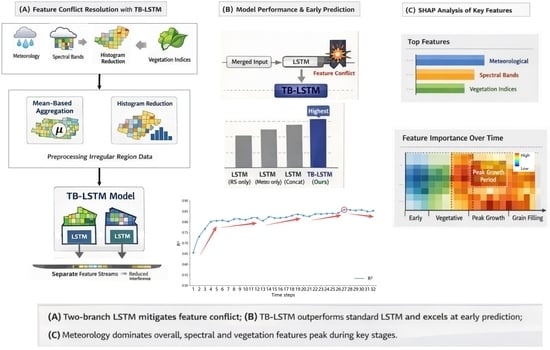
Graphical Abstract

1. Introduction

Wheat is one of the three major staple crops in China, and accurately estimating its yield in a timely manner is critical for formulating grain policies, price regulation, and trade facilitation. Winter wheat yield is influenced by a complex interplay of climatic, soil, and management factors, which exhibit significant nonlinear spatiotemporal variability, posing substantial challenges for yield estimation [1,2,3,4,5].
Traditional approaches to estimating regional wheat yields encompass statistical models [6], machine learning techniques [7], and crop mechanistic models [8]. Statistical models and conventional machine learning techniques generally suffer from constrained parameter capacities and limited generalizability [9], while crop mechanism models demand extensive, hard-to-access parameters and involve costly data assimilation processes [10]. In the era of remote sensing big data, vast observational datasets are characterized by their volume, diversity, dynamic variability, and redundancy, making them extensively applicable to tasks such as crop yield estimation [11]. However, the limitations of traditional methods severely restrict the ability to extract valuable information from large datasets and hinder the effective exploration of complex nonlinear relationships between features and yields. Deep learning, with its powerful capacity to learn and manage complex nonlinear interactions, renders it particularly well-suited for tackling the multifaceted nonlinear problems inherent in crop yield estimation [12]. Compared to statistical and machine learning models, deep learning models typically achieve superior yield estimation performance [13,14,15,16,17,18].
For winter wheat yield estimation at the county level, administrative boundaries often exhibit irregular shapes [19], making it difficult to directly input remote sensing images into mainstream models (e.g., CNNs [20] or LSTMs [21]). To address this challenge, two strategies are often employed to address the challenge. One is Mean Aggregation (MA). This strategy calculates the average value of all pixels within an administrative unit as model input [22,23]. For example, Jiang et al. [24] developed an LSTM model using mean-aggregated meteorological and remote sensing data for county-level maize yield estimation, achieving higher accuracy than statistical and Random Forest (RF) models. Extracting multi-source satellite and meteorological time series from the time series of the continental United States (CONUS) as well as the corn, soybean and wheat production data from the United States Department of Agriculture for design and training, the LSTM model has a high accuracy (R2 > 0.56), and among all crop models, the performance of the multi-source combination is superior to that of the single-variable model [25]. Similarly, Wang et al. [26] proposed a dual-branch deep learning model, where mean-aggregated remote sensing and meteorological data were fed into a dynamic branch, while mean-aggregated soil data were input into a static branch. The merged features from both branches were used for yield prediction. In China’s winter wheat belt, this model achieved an R2 of 0.77 and RMSE of 721 kg/ha. However, mean aggregation only reflects the average pixel value within an administrative unit and ignores intra-unit variability.
The other one is Histogram-Based Dimensionality Reduction (HBDR). This strategy converts pixel values within an administrative unit into a 2D distribution histogram as model input. You [27] utilized histogram dimensionality reduction to construct deep learning networks (CNN and RNN) for crop yield estimation and achieved high accuracy. Zhou et al. [28] and Liu et al. [29] conducted municipal- and county-level winter wheat yield estimation studies based on CNN models with the HBDR strategy, also achieving favorable results. Compared to mean aggregation, histogram-based dimensionality reduction better preserves pixel value distribution information, making it widely adopted for administrative unit-based yield estimation. However, this method requires a sufficient number of pixels per unit to ensure its effectiveness; low-spatial-resolution or small-area applications may fail to generate representative histograms.
Despite the widespread use of these two preprocessing strategies, their impacts on final yield estimation results have not been thoroughly investigated, and the suitability of specific strategies for different data types remains to be fully evaluated.
To address these gaps, this study utilized MOD09A1 reflectance data, vegetation indices, meteorological data, and county-level winter wheat yield statistics (2001–2018) from 363 counties in China to estimate regional winter wheat yield. Sample datasets were generated using both histogram-based dimensionality reduction (for remote sensing data) and mean aggregation (for meteorological data), combining these two heterogeneous temporal data types. This study aims to address the following research questions:
  • Can conventional LSTM models effectively extract meaningful features from heterogeneous temporal data (e.g., remote sensing and meteorological data) for large-scale county-level winter wheat yield estimation?
  • How compatible are features derived from different preprocessing strategies or data types within LSTM models?
  • How do different data types influence estimation accuracy, and how far in advance can the model provide accurate yield predictions relative to the harvest date?

2. Materials and Methods

2.1. Study Area

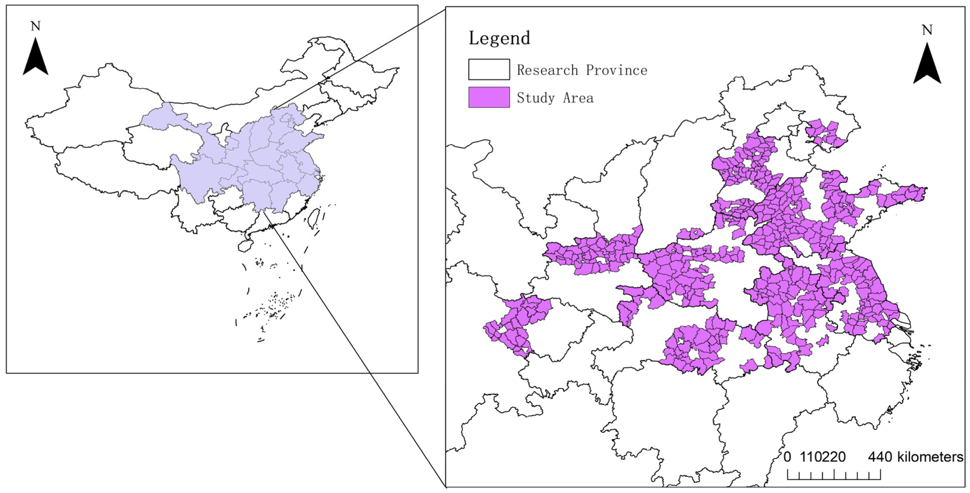
The study area encompasses China’s primary winter wheat-producing regions (106–122°E, 29–40°N), spanning eight provinces: Hebei, Henan, Shandong, Jiangsu, Anhui, Hubei, Shaanxi, and Shanxi (Figure 1). Geographically, the region is divided into northern and southern zones. The northern production area lies south of the Great Wall and north of the Qinling–Huaihe Line, characterized by a temperate continental monsoon climate. The southern production area lies south of the Huaihe River, featuring a subtropical monsoon climate.

2.2. Datasets and Preprocessing

2.2.1. Reflectance Data

Surface reflectance, which reflects soil moisture and crop growth conditions [30,31], was obtained from MOD09A1 data provided by Google Earth Engine (GEE) (https://code.earthengine.google.com/, accessed on 10 September 2025) [32]. Due to variations in winter wheat phenology across regions, data from October 8 to June 10 of the following year were selected to cover the entire growth cycle. Data were acquired every 8 days, resulting in 32 temporal phases for the full growth cycle.

2.2.2. Vegetation Indices

Spectral indices derived from reflectance data are widely used for monitoring crop growth and estimating yield [33,34]. The vegetation indices (VIs) used in this study are listed in Table 1, where R, G, B, and N represent surface reflectance values for Band 1 (red), Band 4 (green), Band 3 (blue), and Band 2 (near-infrared), respectively.

2.2.3. Meteorological Data

Meteorological conditions significantly influence crop yield [41]. This study utilized daily meteorological data from the China Land Data Assimilation System (CLDAS) [42,43,44], with a spatial resolution of 0.1° and NETCDF format. Key yield-related variables are described in Table 2.

2.2.4. Cropland Mask

Due to the lack of long-term, high-resolution winter wheat distribution data, many studies have successfully used cropland data as a proxy mask for large-scale yield estimation [26,45,46]. This study employed the 500 m resolution cropland data from MCD12Q1 as a winter wheat mask.

2.2.5. Yield Data

County-level winter wheat yield and planted area statistics (2001–2018) were obtained from provincial statistical yearbooks. Given the coarse spatial resolution of MODIS data, only counties with planted areas exceeding 10,000 ha and continuous yield records were selected, resulting in 363 counties (Figure 1) and 6534 valid samples.

2.2.6. Data Preprocessing

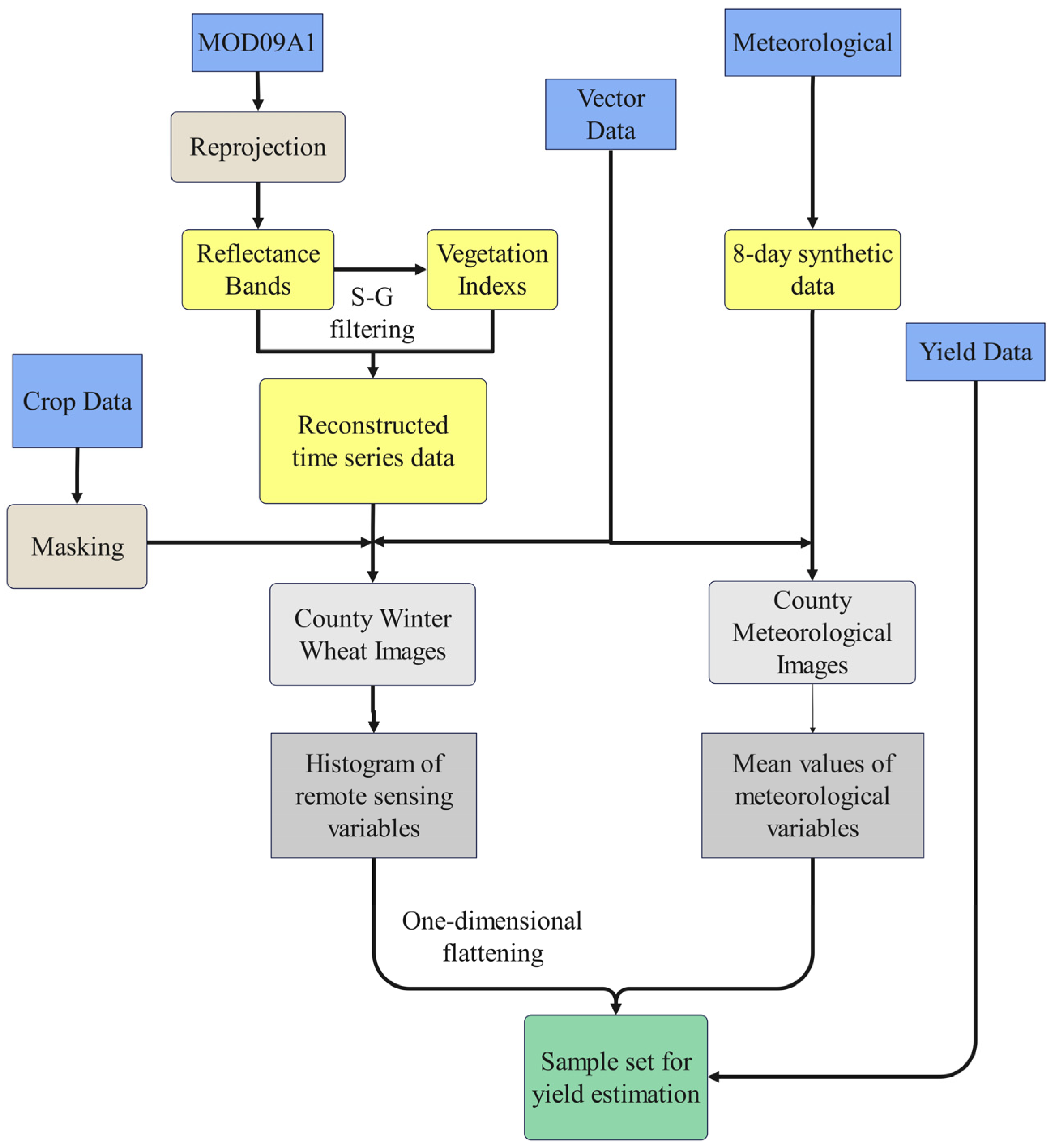
The data preprocessing workflow is depicted in Figure 2. Vegetation indices were calculated based on MOD09A1 reflectance data, and a Savitzky–Golay filter was applied to reconstruct high-quality time series of remote sensing variables, including spectral reflectance and vegetation indices [47,48,49]. Administrative boundary vector data and crop mask data were further used to extract remote sensing data for the winter wheat planting area within each county. To preserve pixel distribution information as fully as possible, HBDR was used to generate histogram features from the remote sensing data of the winter wheat planting area for each county. Histogram features were subsequently flattened into one-dimensional vectors for model input.
Meteorological variables were averaged over each 8-day period to maintain temporal consistency with the remote sensing data. Due to the low spatial resolution (0.1°), HBDR could not be applied to meteorological data. Therefore, Mean aggregation method was used to calculate average values of meteorological variables within each country as model input features.
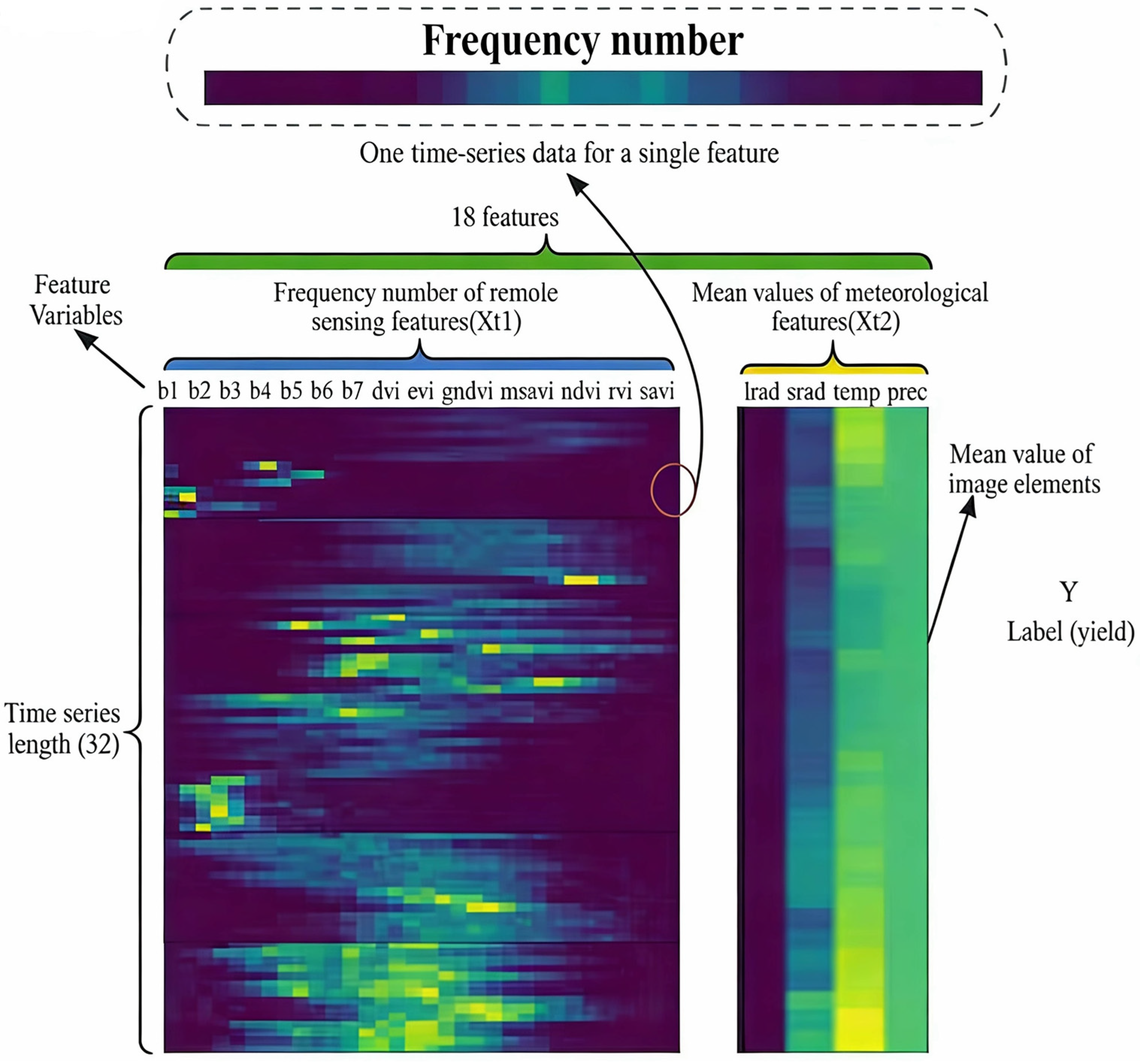
Each sample followed the format: [X1, X2, …, Xt; Y] (Figure 3), where Xt represents the remote sensing and meteorological feature vector at time phase t. The vector Xt consists of two sub-vectors:
  • Xt1 (Remote sensing feature): [b1, b2, b3, b4, b5, b6, b7, evi, ndvi, msavi, savi, dvi, rvi, gndvi], where each element corresponds to the county-level histogram of that feature.
  • Xt2 (Meteorological feature): [lrad, srad, temp, prec], where each element is the county-level mean of that feature.
The time-series length was 32 phases. By applying mean aggregation (for meteorological data) and histogram-based dimensionality reduction (for remote sensing data), this approach resolved the challenge of directly inputting irregular imagery into deep learning models.

2.3. Deep Learning Models

The deep learning models were implemented using the PyTorch 2.4.1 framework. Model parameters were optimized using the mean squared error (MSE) loss function, which calculates the average squared difference between predicted and observed values. Samples were randomly split into training and testing sets at an 8:2 ratio. The initial learning rate was set to 0.0001, with the Adam optimizer employed for loss minimization. ReLU activation functions were applied in the network, and training proceeded for 300 epochs, with the best-performing model saved during the process.

2.3.1. LSTM Network Structure

The LSTM model is highly effective at capturing temporal dependencies, making it widely applicable in crop yield estimation [50]. In this study, the input data consisted of histogram-derived remote sensing features and mean-aggregated meteorological features. An LSTM baseline model was constructed to evaluate its ability to extract meaningful features from these heterogeneous temporal data for county-level winter wheat yield estimation. The benchmark LSTM model contained 32 units, two fully connected (FC) layers, and a Dropout layer. The optimal hyperparameters of the LSTM model are described in Section 3.3.1.

2.3.2. TB-LSTM Model

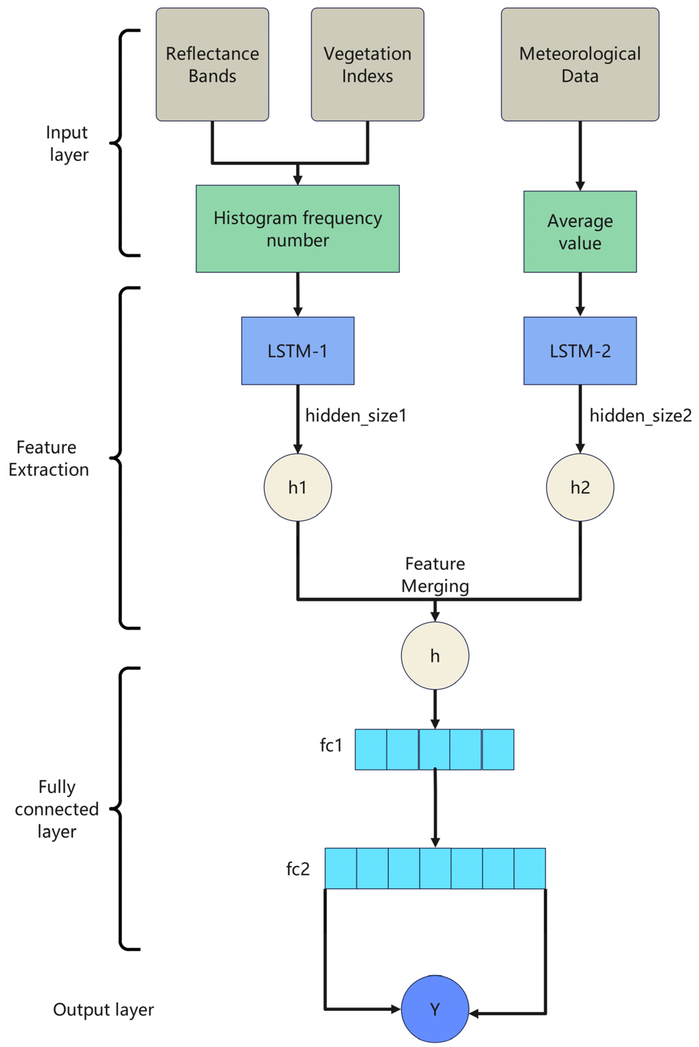
To investigate the effects of different network structures on yield estimation and the compatibility of features obtained through different preprocessing strategies, a Two-Branch Long Short-Term Memory (TB-LSTM) model was developed (Figure 4). The model comprises two branches, each containing an LSTM feature extraction submodule:
  • Branch 1: Extracted temporal features from histogram-based remote sensing data.
  • Branch 2: Extracted temporal features from mean-aggregated meteorological data.
The high-level features from both branches were concatenated and fed into an FC layer for final yield prediction.

2.4. Model Evaluation Metrics

Model performance was assessed using the coefficient of determination (R2), root mean square error (RMSE), and mean absolute error (MAE), calculated as follows:
R 2 = 1 i = 1 n ( y i y ^ i ) 2 i = 1 n ( y i y ¯ ) 2
R M S E = 1 n i = 1 n ( y i y ^ i ) 2
M A E = 1 n i = 1 n | y i y ^ i |
where yi refers to observed yield for county i, y ^ i refers to predicted yield (kg/ha), and y ¯ refers to observed yield. Higher R2 and lower RMSE/MAE values indicate better performance.

2.5. SHAP Analysis

SHAP (SHapley Additive Explanations) is an interpretable machine learning framework introduced by Lundberg and Lee in 2017, grounded in the Shapley value concept derived from cooperative game theory. This method quantitatively attributes the prediction outcome of a machine learning model to individual input features by decomposing the model output into additive feature contributions, thereby providing a principled and locally accurate explanation for the otherwise opaque “black-box” decision process [51,52,53,54].
SHAP offers interpretability support for various types of models, including complex ones such as deep learning and ensemble learning. In this study, SHAP is employed to quantify the contribution across different temporal stages to winter wheat yield prediction. This analysis aims to reveal the key growth stages captured by the model and identify core influencing factors, thereby providing scientific support for model refinement and agricultural production decision-making.

3. Results

3.1. The Phenomenon of “Feature Conflict”

Remote sensing time-series data processed through histogram dimensionality reduction reflect both the magnitude and distribution of pixel values within counties, whereas meteorological time-series data processed through mean aggregation only represent the averaged values of meteorological variables at the county level. This section investigates whether the baseline LSTM model can effectively extract features from these two heterogeneous types of time-series data for county-level winter wheat yield estimation.
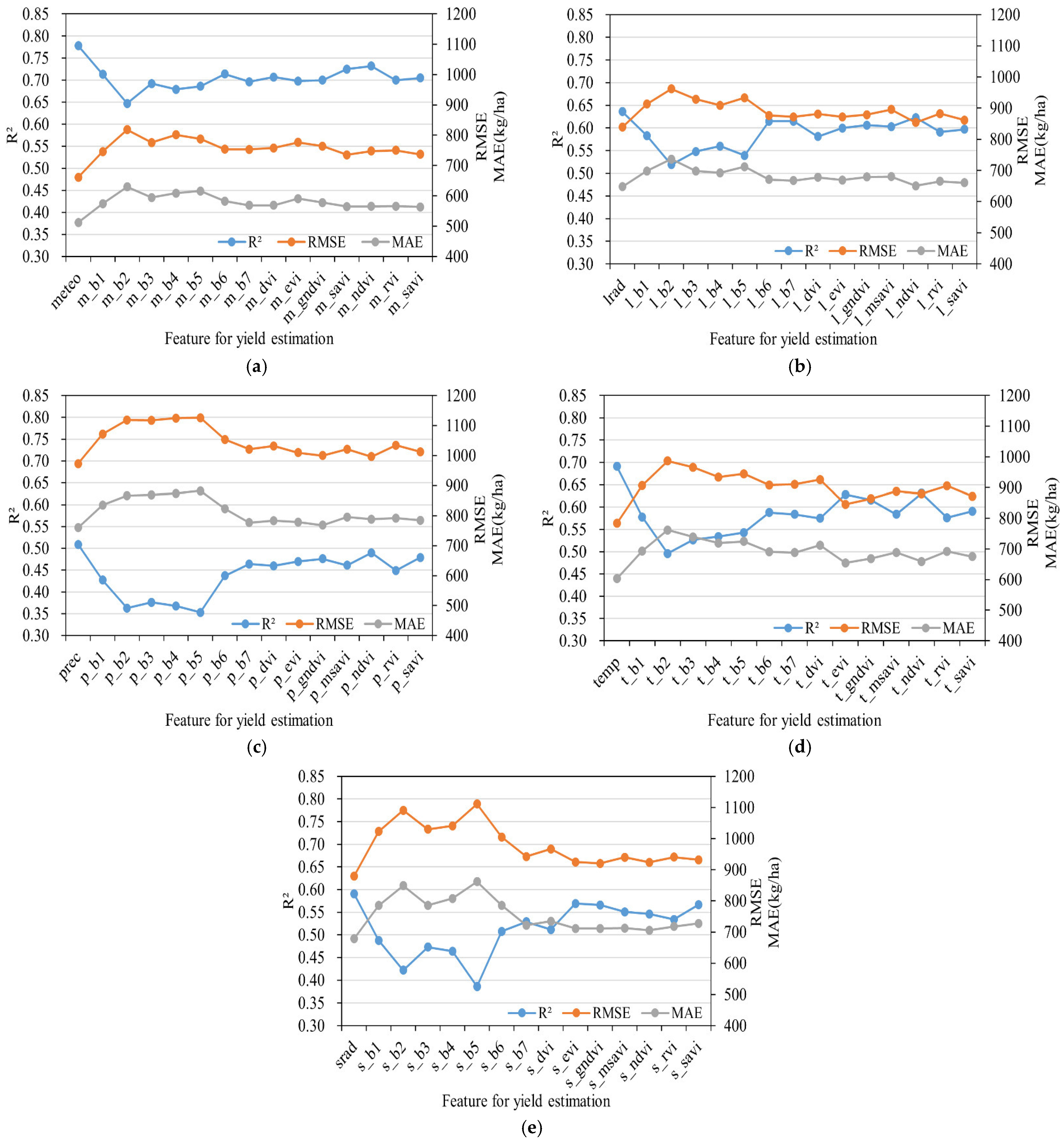
Based on the LSTM model described in Section 2.3.1, any single remote sensing feature was introduced as additional input data alongside meteorological features, and changes in yield estimation accuracy were compared before and after incorporating the remote sensing feature. The results are shown in Figure 5. Here, “meteo” represents all meteorological features (lrad, srad, temp, and prec), while “l,” “s,” “t,” and “p” denote lrad, srad, temp, and prec, respectively.
When trained solely on meteorological data (“meteo”), the LSTM model achieved an R2 of 0.774, RMSE of 633.622 kg/ha, and MAE of 474.126 kg/ha. However, when any single remote sensing feature was incorporated, the model’s performance declined (R2: 0.647–0.732; RMSE: 735.378–818.382 kg/ha; MAE: 563.348–629.753 kg/ha). This indicates that combining meteorological time-series data with any remote sensing time-series data in an LSTM model leads to “feature conflict.”
Further experiments were conducted by pairing individual meteorological features with remote sensing features to assess their compatibility. The results revealed that combining longwave radiation (lrad) with remote sensing features resulted in R2 values between 0.519 and 0.623 and RMSE values between 853.815 and 961.969 kg/ha, compared to an R2 of 0.636 and RMSE of 838.923 kg/ha when using lrad alone.
Similarly, when srad alone was used as input, the model yielded R2 = 0.591, RMSE = 879.022 kg/ha, and MAE = 678.689 kg/ha. Adding any remote sensing feature resulted in reduced accuracy (R2: 0.386–0.569; RMSE: 920.602–1111.574 kg/ha; MAE: 705.291–861.732 kg/ha).
For temp as the sole input feature, the model achieved R2 = 0.691, RMSE = 783.883 kg/ha, and MAE = 603.053 kg/ha. Incorporating any remote sensing feature led to performance degradation (R2: 0.496–0.631; RMSE: 845.194–986.767 kg/ha; MAE: 654.045–761.751 kg/ha).
When prec alone was used as input, the model obtained R2 = 0.509, RMSE = 972.984 kg/ha, and MAE = 759.822 kg/ha. Combining prec with any remote sensing feature further reduced accuracy (R2: 0.353–0.49; RMSE: 996.256–1126.062 kg/ha; MAE: 768.218–882.324 kg/ha).
These results consistently demonstrate that introducing any remote sensing feature alongside individual meteorological variables in the LSTM model leads to varying degrees of performance degradation. This conclusively confirms the existence of “feature conflict” in LSTM models when processing mean-aggregated meteorological data and histogram-based remote sensing data, preventing effective extraction of yield estimation features from these heterogeneous data types.

3.2. The TB-LSTM Model for Resolving “Feature Conflict”

A natural solution to the phenomenon of “feature conflict” is to process different types of input features separately. In light of this, a Two-Branch Long Short-Term Memory (TB-LSTM) model was designed in this study. The TB-LSTM model contains two distinct branches, with one branch dedicated to processing remote sensing features derived from histogram dimensionality reduction and the other branch focused on meteorological features processed via the mean-value method. After independent processing, the extracted high-level features from the two branches are merged and passed through fully connected layers to output yield predictions.
To ensure comparability with the baseline LSTM model, the parameters of the TB-LSTM model were configured identically. The hidden sizes of the two branches were set to 256, while the combined feature dimension after merging was maintained at 512 to match the input size of the fully connected layers. The batch size, dropout rate, and learning rate were kept consistent with those of the baseline LSTM model.
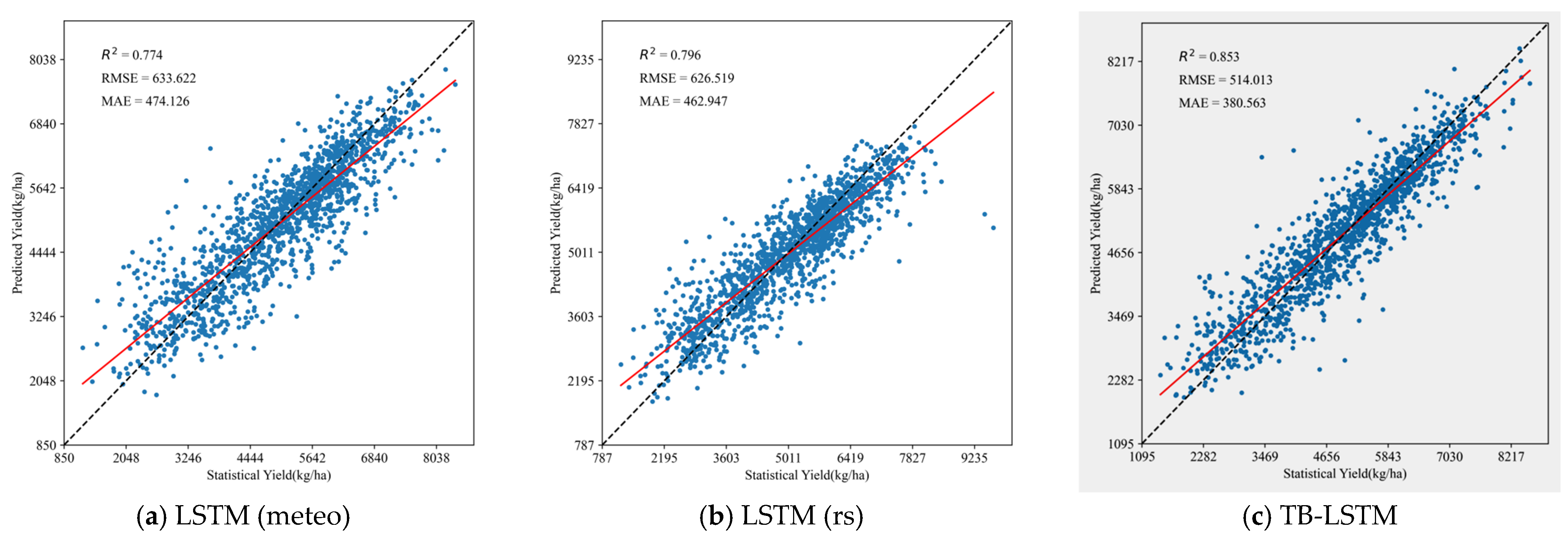
Experimental results revealed that the TB-LSTM model significantly outperformed the baseline LSTM model in yield estimation accuracy. When combining remote sensing and meteorological features, the TB-LSTM model achieved an average R2 of 0.853, RMSE of 514.013 kg/ha and MAE of 380.563 kg/ha. These metrics were consistently better than those of the baseline LSTM model (R2: 0.774–0.796; RMSE: 626.519–633.622 kg/ha; MAE: 462.947–474.126 kg/ha), which suffered from feature conflict when integrating the same types of input features.
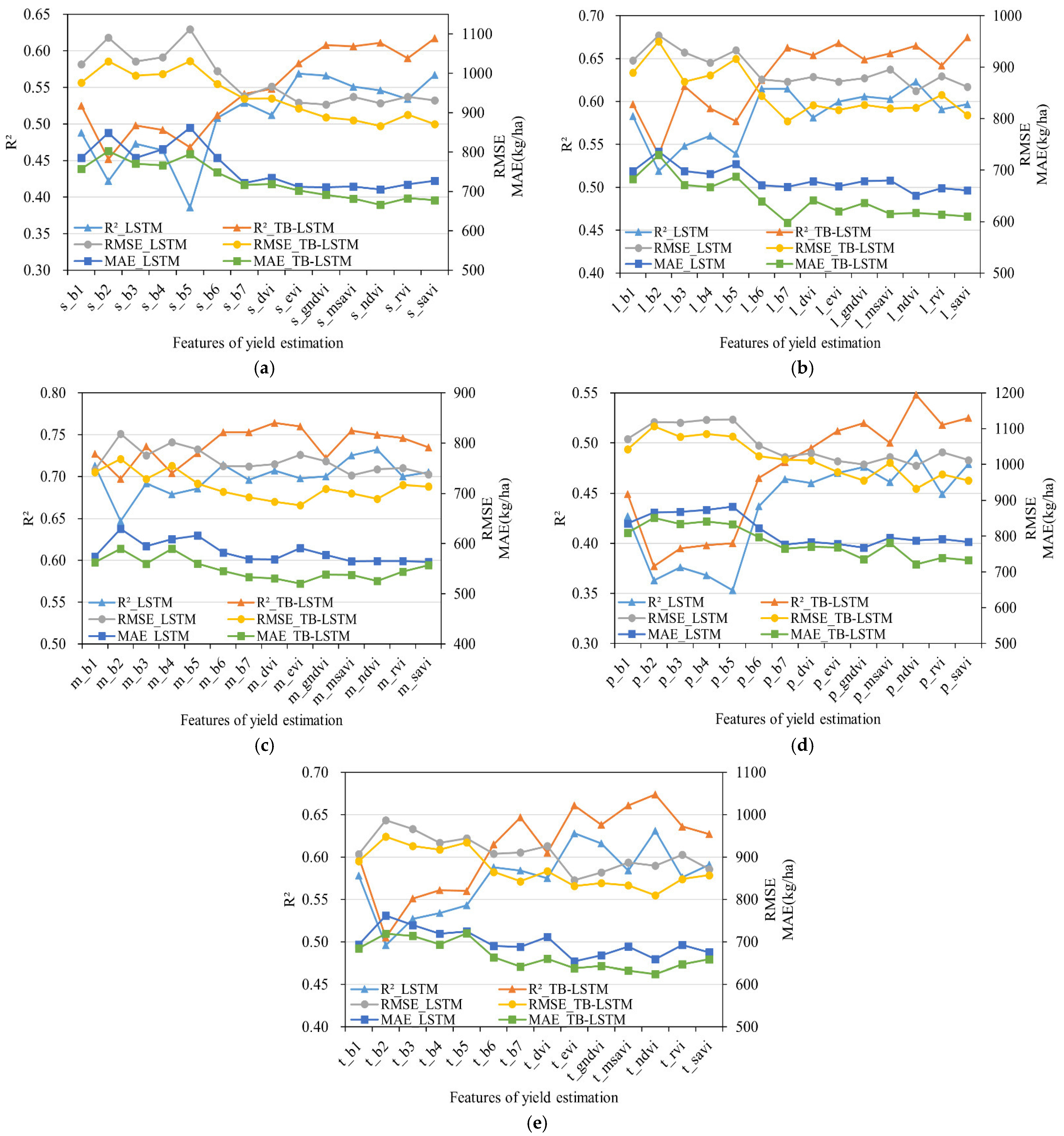
To further validate the ability of the TB-LSTM model to handle heterogeneous data, additional experiments were conducted by fusing individual meteorological features with remote sensing features. The results are shown in Figure 6. TB-LSTM model achieved superior estimation accuracy compared to the baseline LSTM model across all combinations of features. For instance, when combining longwave radiation (lrad) with individual remote sensing features, the TB-LSTM model achieved R2 values between 0.538 and 0.675, RMSE values between 794.804 and 950.136 kg/ha, and MAE values between 597.400 and 729.118 kg/ha. In contrast, the baseline LSTM model exhibited inferior performance, with R2 values ranging from 0.519 to 0.623, RMSE values ranging from 853.815 to 961.969 kg/ha, and MAE values ranging from 650.808 to 736.369 kg/ha.
For srad paired with remote sensing features, TB-LSTM achieved R2: 0.452–0.617; RMSE: 865.727–1030.703 kg/ha; MAE: 665.770–802.06 kg/ha, showing improvement over LSTM (R2: 0.386–0.569; RMSE: 920.602–1111.574 kg/ha; MAE: 705.291–861.732 kg/ha).
For temp combined with remote sensing features, TB-LSTM yielded R2: 0.505–0.674; RMSE: 810.009–947.924 kg/ha; MAE: 624.223–720.016 kg/ha, surpassing LSTM (R2: 0.496–0.631; RMSE: 845.194–986.767 kg/ha; MAE: 654.045–761.751 kg/ha).
For prec paired with remote sensing features, TB-LSTM obtained R2: 0.377–0.548; RMSE: 932.707–1107.128 kg/ha; MAE: 721.466–851.168 kg/ha, demonstrating better performance than LSTM (R2: 0.353–0.49; RMSE: 996.256–1126.062 kg/ha; MAE: 768.218–882.324 kg/ha).
Overall, the TB-LSTM model successfully mitigated the issue of feature conflict by independently processing remote sensing and meteorological features, thereby enabling the effective extraction of meaningful information from both data sources. This innovative model architecture provides a robust framework for integrating heterogeneous temporal data in crop yield estimation tasks.

3.3. Winter Wheat Yield Estimation Using TB-LSTM

3.3.1. Hyperparameter Configuration for TB-LSTM and Benchmark Models

To further assess the effectiveness of the TB-LSTM model, its yield estimation accuracy was compared against baseline models under varying experimental conditions. The optimal hyperparameters of models are shown in Table 3. The number of hidden layer nodes is kept comparable across all models to ensure their comparability.

3.3.2. Performance of TB-LSTM and Benchmark Models

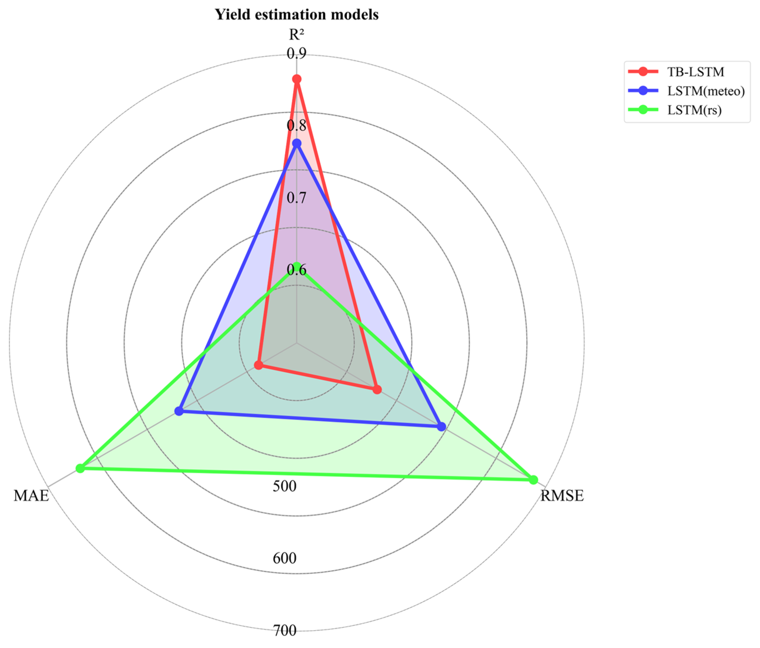
The TB-LSTM model’s ability to integrate heterogeneous data sources—including spectral reflectance, vegetation indices, and meteorological data—led to significantly enhanced prediction performance (Figure 7).
When all available features were included, the TB-LSTM model achieved an average R2 of 0.853, indicating that the model could explain 85.3% of the variance in the actual yield data. Correspondingly, the RMSE and MAE were measured at 514.013 kg/ha and 380.563 kg/ha, respectively, demonstrating a substantial reduction in prediction error (Figure 8). By comparison, the baseline LSTM models using only meteorological features or only remote sensing features achieved lower accuracy. The average R2 values for LSTM models were 0.774 and 0.796, respectively, with RMSE values of 633.622 kg/ha and 626.519 kg/ha, and MAE values of 474.126 kg/ha and 462.947 kg/ha.
Additionally, the TB-LSTM model’s performance remained consistent across multiple independent experiments. The variance in R2 values among experiments was less than 0.028, while the variance in RMSE and MAE values was 41.49 kg/ha and 42.793 kg/ha, respectively. These results highlight the robustness and reliability of the TB-LSTM model in yield estimation tasks.
The incorporation of diverse data sources in the TB-LSTM model provided critical advantages. For example, the combined use of spectral reflectance, vegetation indices, and meteorological data yielded the highest estimation accuracy. When certain data sources were excluded (e.g., vegetation indices or spectral reflectance), the model’s accuracy decreased but remained superior to that of baseline models. This finding underscores the importance of integrating multi-source data to capture complex interactions influencing crop yield.
In summary, the TB-LSTM model demonstrated significant improvements in yield estimation accuracy compared to traditional LSTM models. Its robust performance across various experimental conditions further validated its potential as a reliable tool for large-scale agricultural monitoring and decision-making.

3.3.3. Performance of TB-LSTM Model with Different Input Features

Using the TB-LSTM framework, we evaluated yield estimation performance across different input feature combinations and assessed relative contributions of data sources (Table 4). Based on evaluation metrics, the combinations ranked as “R + VI + M” (R2: 0.853; RMSE: 514.013 kg/ha; MAE: 380.563 kg/ha) > “M + VI” (0.848, 523.328, 377.097) > “M + R” (0.846, 527.351, 384.213), where R denotes reflectance bands, VI vegetation indices, and M meteorological data.
The highest accuracy was achieved when incorporating all three data types in the TB-LSTM model (R2: 0.853; RMSE: 514.013 kg/ha; MAE: 380.563 kg/ha), surpassing machine learning models (Ridge Regression, Support Vector Machine, Random Forest, and Light Gradient Boosting), which achieved R2 between 0.57 and 0.77.

3.3.4. Early Prediction Capability of TB-LSTM

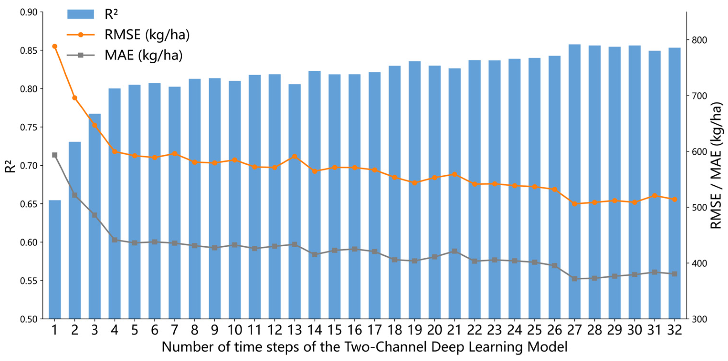
Figure 9 illustrates the variation in crop yield estimation accuracy of the TB-LSTM model as multi-temporal data are progressively incorporated, demonstrating its capability for early yield prediction. Overall, as multi-temporal data are incorporated, the model accuracy initially increases rapidly, then the rate of improvement slows down, though it continues to show an upward trend. The proposed TB-LSTM model achieved robust early prediction capability, attaining optimal accuracy (R2 = 0.868, RMSE = 487.327 kg/ha, MAE = 361.353 kg/ha) using only the first 27 time phases, thereby enabling reliable county-level yield prediction 48 days before harvest with performance comparable to models utilizing the full temporal datasets.

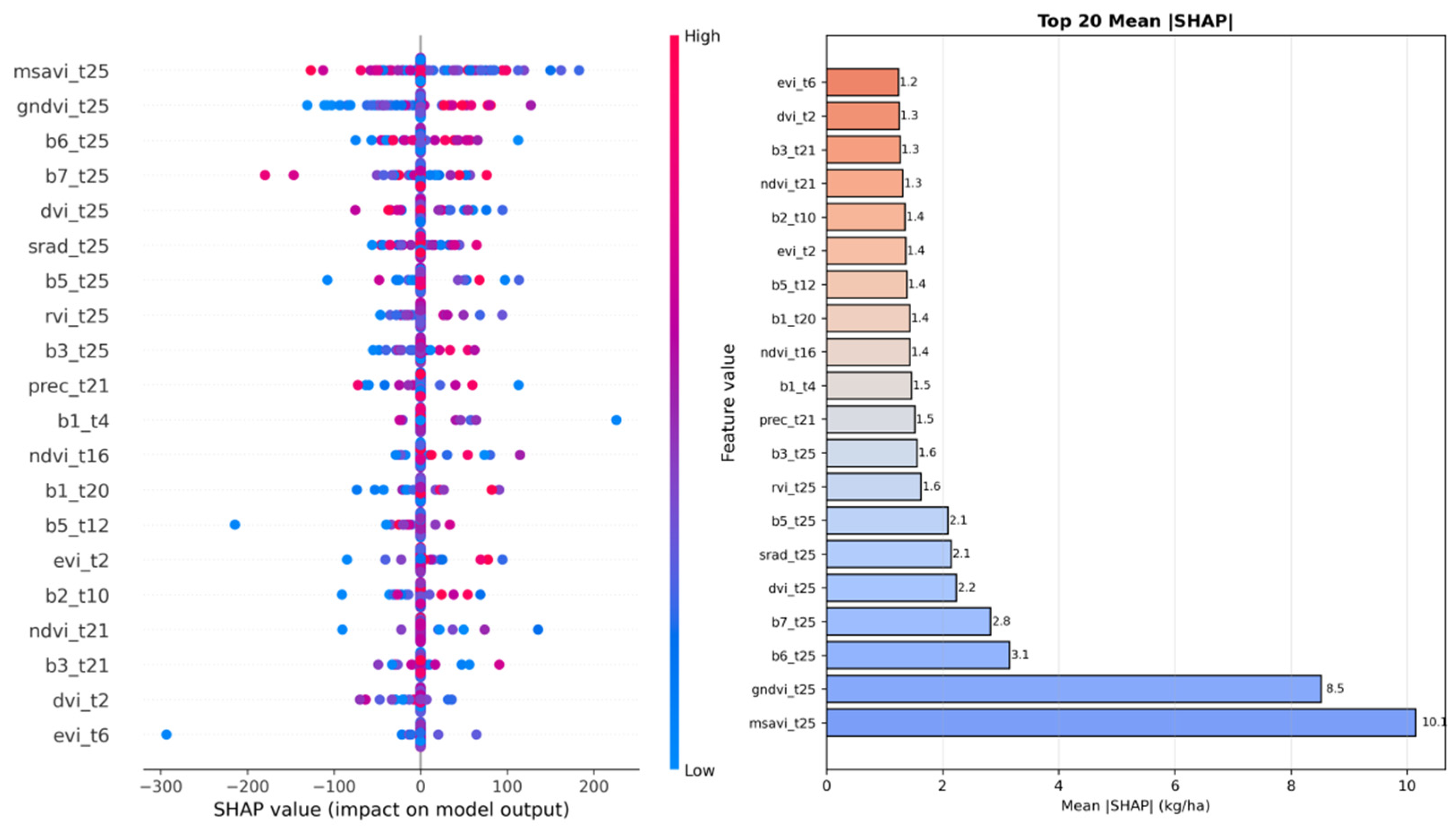
3.4. Model Interpretability Analysis Based on the SHAP Method

Based on the SHAP method, the contribution of each input feature in the TB_LSTM model was quantified, and the top 20 features were ranked and analyzed quantitatively. The detailed experimental results are presented in Figure 10. The feature msavi_t25 (the MSAVI of winter wheat at the 25th phase) exhibited the highest contribution, with a SHAP value of 10.15. This temporal stage corresponds to a critical window for yield formation. By minimizing soil background interference, MSAVI effectively reflects canopy structural dynamics and biomass accumulation during the jointing–booting stages of winter wheat, thereby exerting a significant influence on yield prediction.
The second most important feature was gndvi_t25, with a SHAP value of 8.52. This index effectively captures leaf nitrogen status and photosynthetic activity in the pre-heading stage of winter wheat, which is the key period for determining spikelet number, thus making a substantial contribution to yield estimation. The two most influential features are both vegetation indices, confirming that vegetation indices, through band-combination operations, provide richer and more information for yield prediction.
Among the reflectance features, b6_t25 and b7_t25 ranked among the highest in terms of contribution, with SHAP values of 3.15 and 2.83, respectively. As mid-infrared bands, Bands 6 and 7 are sensitive to crop canopy water content and leaf temperature. Their high contributions at the 25th time step indicate that the model likely makes effective use of information related to water stress. The SHAP values of b5_t25 and b3_t25 were 2.09 and 1.56, respectively, highlighting the value of red-edge and blue bands in monitoring crop physiological status during critical growth stages.
The contributions of meteorological factors were relatively concentrated. srad_t25 exhibited a SHAP value of 2.15, and its high contribution during the booting stage suggests that photosynthetically active radiation directly drives the rate of dry matter accumulation. prec_t21 showed a contribution of 1.52, corresponding to the mid-jointing stage, confirming the constraining effect of water supply on stem elongation and young spike differentiation.
From a temporal perspective, the 25th time phase (approximately mid-April, spanning the jointing–booting–heading stages) represents the core window for yield estimation. All of the top eight ranked features were concentrated at this time phase, corroborating that this period constitutes an information-intensive phase for yield prediction and providing interpretable scientific evidence to support agricultural production decision-making.

4. Discussion

4.1. Impact of Different Data on the Accuracy of the TB-LSTM Model

The dataset employed in this study combines meteorological features processed through the mean aggregation with remote sensing features extracted using histogram dimensionality reduction. The mean aggregation summarizes the average values of meteorological variables within counties, effectively representing the overall meteorological conditions. However, it does not capture the spatial variability among grid cells. In contrast, the histogram dimensionality reduction approach encodes both the values and the distribution of remote sensing variables within counties, preserving key spatial details.
Previous studies have demonstrated the advantages of histogram dimensionality reduction over mean aggregation methods. For instance, Liu [48] applied histogram dimensionality reduction to MOD09A1 data in Henan Province and achieved higher yield estimation accuracy compared to the mean-value method. Specifically, the histogram-based reflectance data outperformed the mean aggregation method with RMSE values of 383 kg/ha versus 464 kg/ha, respectively.
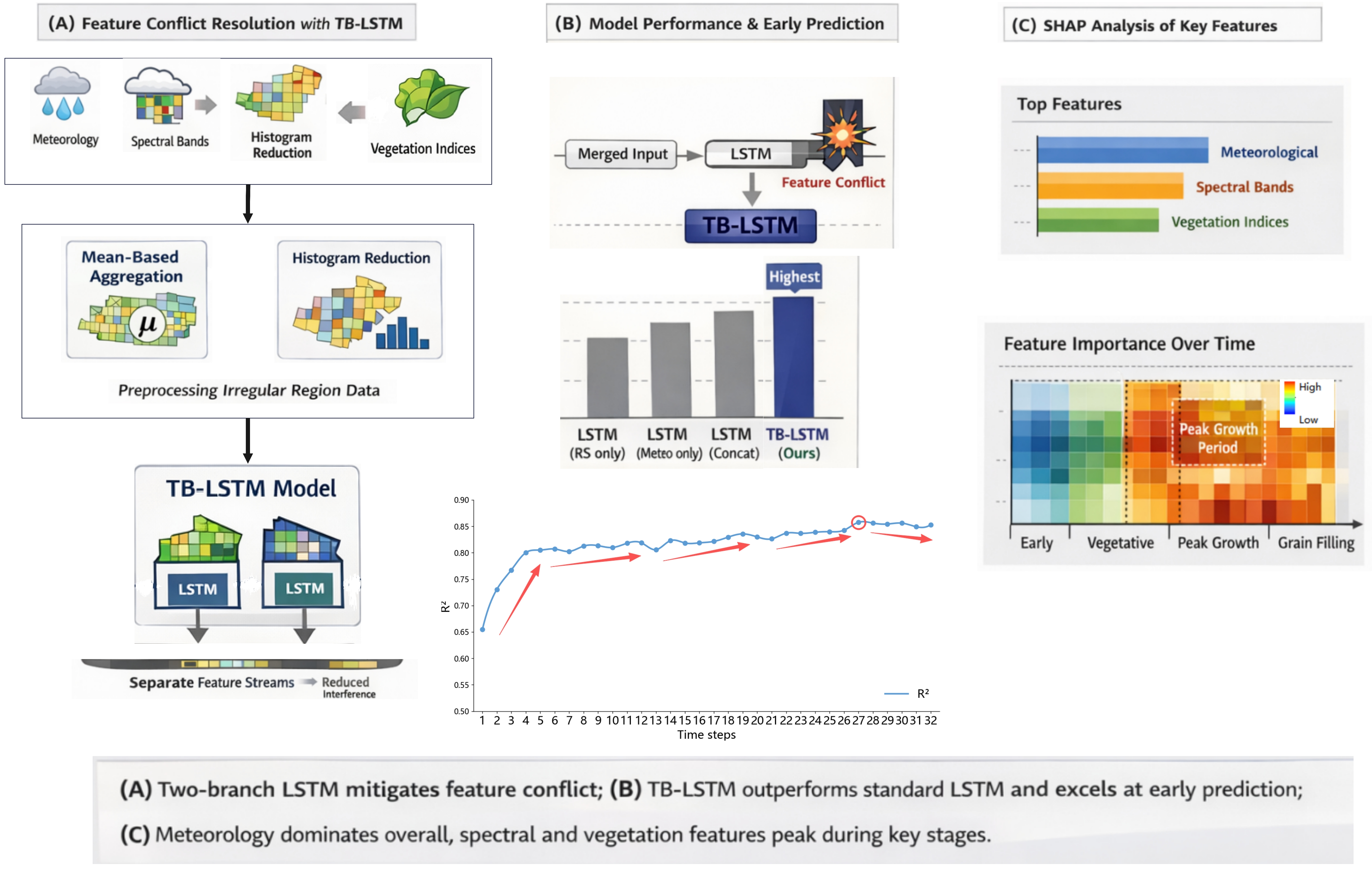
Building upon previous work, our study incorporated meteorological data into yield estimation models. However, due to their coarse spatial resolution, histogram methods were inapplicable to meteorological data, necessitating mean aggregation. When feeding both histogram-derived frequencies and mean-aggregated values into LSTM models, these heterogeneous temporal data types failed to provide complementary features for yield estimation. Instead, they induced “feature conflict,” preventing effective extraction of meteorological and remote sensing temporal features and consequently degrading model performance. Our proposed TB-LSTM architecture successfully resolved this conflict through separate branch processing [26,55,56].
The experimental results revealed that while meteorological data provided the most significant contribution to yield estimation, the addition of histogram-based remote sensing data further enhanced the model’s performance. This indicates that the integration of diverse data sources enables the TB-LSTM model to better capture the complex factors influencing crop yield.
Excluding either reflectance or vegetation indices resulted in slightly reduced accuracy but still demonstrated the value of multi-source data integration. These results underscore the complementary nature of remote sensing and meteorological data in improving yield estimation accuracy.

4.2. Early Yield Prediction Capacity of TB-LSTM Model

Crop growth is a cumulative process, where biomass progressively accumulates and determines final yield [57]. Stressors experienced during early growth stages can significantly impact later growth and eventual yields [58]. Therefore, accurate early yield prediction is essential for effective agricultural management. In this study, the TB-LSTM model’s early prediction capability was systematically evaluated by incrementally increasing the number of temporal phases included in training [59].
During phases 1–4, winter wheat undergoes the germination and emergence stages, during which cropland gradually transitions from bare soil to being covered by wheat leaves. As additional temporal observations are incorporated into the training dataset, the yield estimation performance of the TB-LSTM model improves progressively.
For phases 5–27, winter wheat experiences the tillering, overwintering, regreening, jointing, and booting stages, during which the overall accuracy of the yield estimation model exhibits a steadily increasing trend. During the tillering stage, crop growth is relatively slow and highly sensitive to environmental variability. In the overwintering stage, winter wheat growth largely ceases, whereas in the regreening stage, leaf growth resumes but the canopy remains mostly prostrate. The regreening–jointing stage represents a critical transition in winter wheat development. With rising spring temperatures, crop growth accelerates markedly, stems begin to elongate, and overall growth rates increase. During this period, remote sensing data can effectively capture pronounced growth dynamics, such as substantial increases in vegetation indices and rapid biomass accumulation. These features contribute strongly to yield prediction, leading to improved estimation accuracy. The booting–heading stage constitutes another key phase in winter wheat development. Remote sensing observations during this period capture further structural and phenological changes, including spike formation and flowering, which provide critical information for predicting final yield. As a result, estimation accuracy could continue to improve.
When the time phase reaches 28–32, winter wheat enters the heading as well as the grain-filling and maturity stages. During this phase, leaf development becomes pronounced and wheat spikes are fully formed. With the continued extension of the temporal training data, yield estimation accuracy reaches its peak and remains at a high level.
Yield prediction is commonly based on statistical models and machine learning approaches that rely on key growth stages. Fu et al. [60] calculated multiple vegetation indices from wheat canopy reflectance and used the optimal indices as model inputs to develop yield prediction models based on simple linear regression, multiple linear regression, stepwise multiple linear regression, partial least squares regression, artificial neural networks, and random forest (RF). The results demonstrated that machine learning methods outperform traditional statistical models in yield prediction. Among them, an RF model constructed using NDVI at the jointing, heading, flowering, and grain-filling stages was identified as the optimal wheat yield prediction model, achieving an R2 of 0.78.
Using the TB-LSTM yield estimation model and incorporating data from the first 27 time steps, this study achieved a prediction accuracy of R2 0.868, with an RMSE of 487.327 kg/ha and an MAE of 361.353 kg/ha, enabling county-level winter wheat yield prediction 48 days in advance. This level of accuracy is comparable to that obtained using data from all time steps. Compared with traditional statistical models and conventional machine learning approaches, the TB-LSTM model developed in this study demonstrates superior performance in yield prediction.
SHAP analysis further confirms that feature contributions exhibit pronounced phenological characteristics throughout the entire growth cycle of winter wheat. Features from phases 20–28 (jointing–booting–heading stages) consistently show higher average SHAP values, corresponding to the critical period of winter wheat yield formation and indicating that the model is most sensitive to feature information during this stage. Features from time steps 10–19 (overwintering–regreening stages) exhibit the second-highest contributions; during this period, the features primarily reflect crop stress tolerance and growth recovery conditions, which exert an important cumulative effect on yield formation.
In contrast, features from phases 1–9 (germination–tillering stages) and 29–32 (grain filling–maturity stages) show relatively lower contributions. For the early growth stage, the influence of initial growth conditions can be compensated by features from subsequent stages, whereas during the late grain-filling stage, yield has largely stabilized, and additional feature information contributes less to the prediction results. By quantifying the contribution of each feature, the SHAP method elucidates the prediction mechanism of the TB-LSTM model and verifies its scientific rationality.
The ability to deliver accurate predictions 48 days ahead of harvest demonstrates the practical utility of the TB-LSTM model. By identifying critical growth stages and leveraging detailed temporal data, the model enables proactive decision-making, such as targeted interventions and optimized resource allocation. Furthermore, this early prediction capability supports strategic planning for market supply and demand [61].

5. Conclusions

Based on remote sensing data, meteorological data, and yield data from China’s major wheat-producing regions from 2001 to 2018, winter wheat yield estimation at the county scale was conducted. The HBDR and MA methods were employed to extract county-level remote sensing and meteorological features, respectively. The yield estimation performance of the baseline LSTM model and the proposed TB-LSTM model was compared, and feature conflict was resolved using the proposed model. The SHAP method was applied to analyze the contribution of different features to yield estimation, and the model’s capability for early-season yield prediction was discussed. The main conclusions are as follows:
The LSTM model exhibited a “feature conflict” phenomenon, where the heterogeneous characteristics of meteorological data (mean-aggregated) and remote sensing data (histogram-based) interfered with each other during feature extraction, ultimately constraining model performance. By leveraging separate processing branches for these distinct data types, the proposed TB-LSTM model successfully resolved the feature conflict issue observed in traditional LSTM models. The TB-LSTM model demonstrated superior performance, achieving an R2 of 0.853 and reducing RMSE and MAE values compared to baseline LSTM models.
The integration of meteorological data, spectral reflectance, and vegetation indices proved essential for achieving optimal yield estimation accuracy. Meteorological data provided the most significant contribution, while spectral reflectance and vegetation indices offered complementary information that improved model robustness. When all three data types were utilized simultaneously, the TB-LSTM model achieved peak estimation accuracy (R2: 0.853; RMSE: 516.619 kg/ha; MAE: 378.499 kg/ha).
SHAP analysis confirms that feature contributions exhibit pronounced phenological characteristics throughout the entire growth cycle of winter wheat. The 25th phase (approximately mid-April, spanning the jointing–booting–heading stages) represents the core window for yield estimation.
The TB-LSTM model demonstrated robust early yield prediction capability. Using data from the first 27 time phases (covering growth stages up to heading), the model achieved estimation accuracy of R2 = 0.868, RMSE = 487.327 kg/ha, and MAE = 361,353 kg/ha, successfully predicting yields 48 days before harvest with optimal precision. This capability supports proactive decision-making and resource allocation in agricultural management.
The results of this study emphasize the importance of integrating diverse data sources and leveraging advanced deep learning architectures for crop yield estimation. Future research should focus on incorporating management measures such as fertilization, irrigation, and variety improvement to further enhance the predictive capabilities of the model.

Author Contributions

Conceptualization, B.L.; Methodology, X.W.; Writing—original draft, B.L.; Writing—review & editing, B.Z. (Bin Zhao); Visualization, B.Z. (Bin Zhao); Supervision, B.L. and Z.C.; Project administration, Z.C. and B.Z. (Bing Zhang); Funding acquisition, B.Z. (Bing Zhang). All authors have read and agreed to the published version of the manuscript.

Funding

This research was funded by National Natural Science Foundation of China (grant number 42030111).

Data Availability Statement

The raw data supporting the conclusions of this article will be made available by the authors on request.

Conflicts of Interest

The authors declare no conflict of interest.

References

  1. Wang, N.; Wu, J.; Gu, Y.; Jiang, K.; Ma, X. Factors Influencing the Spatiotemporal Variability in the Irrigation Requirements of Winter Wheat in the North China Plain under Climate Change. Agronomy 2022, 12, 1987. [Google Scholar] [CrossRef]
  2. Ma, S.; Churkina, G.; Gessler, A.; Wieland, R.; Bellocchi, G. Yield gap of winter wheat in Europe and sensitivity of potential yield to climate factors. Clim. Res. 2016, 67, 179–190. [Google Scholar] [CrossRef][Green Version]
  3. Li, B.; Wang, T.; Meng, F. Double quantitative analysis of the effects of meteorological factors on winter wheat yield at different growth stages based on grey relational analysis. J. Grey Syst. 2018, 30, 31–44. [Google Scholar]
  4. Song, N.; Sun, J.; Wang, J.; Chen, Z.; Liu, Z. Temporal and spatial variation of water requirement of winter wheat and its influencing factors in Henan Province, China. J. Appl. Ecol. 2014, 25, 1693–1700. [Google Scholar]
  5. Wang, K.; Liu, H.; Zhou, X.; Tang, X. Comprehensive Mega-Data Analysis of Water Use Efficiency in Winter Wheat and Its Influencing Factors. Water 2025, 17, 564. [Google Scholar] [CrossRef]
  6. Li, J.; Guo, Q.; Peng, Y. Remote sensing estimation model of Henan province winter wheat yield based on MODIS data. Ecol. Environ. Sci. 2012, 21, 1665–1669. [Google Scholar]
  7. Maimaitijiang, M.; Sagan, V.; Sidike, P.; Hartling, S.; Esposito, F.; Fritschi, F.B. Crop monitoring using satellite/UAV data fusion and machine learning. Remote Sens. 2020, 12, 1357. [Google Scholar] [CrossRef]
  8. Zhuo, W.; Fang, S.; Gao, X.; Wang, L.; Wu, D.; Fu, S.; Wu, Q.; Huang, J. Crop yield prediction using MODIS LAI, TIGGE weather forecasts and WOFOST model: A case study for winter wheat in Hebei, China during 2009–2013. Int. J. Appl. Earth Obs. Geoinf. 2022, 106, 102668. [Google Scholar] [CrossRef]
  9. Shi, W.; Tao, F.; Zhang, Z. A review on statistical models for identifying climate contributions to crop yields. J. Geogr. Sci. 2013, 23, 567–576. [Google Scholar] [CrossRef]
  10. Huang, J.; Gómez-Dans, J.L.; Huang, H.; Ma, H.; Wu, Q.; Lewis, P.E.; Liang, S.; Chen, Z.; Xue, J.; Wu, Y. Assimilation of remote sensing into crop growth models: Current status and perspectives. Agric. For. Meteorol. 2019, 276, 107609. [Google Scholar] [CrossRef]
  11. Zhang, B. Remotely Sensed Big Data Era and Intelligent Information Extraction. Geomatics Inf. Sci. Wuhan Univ. 2018, 43, 1861–1871. [Google Scholar]
  12. Okamura, R.; Iwabuchi, H.; Schmidt, K.S. Feasibility study of multi-pixel retrieval of optical thickness and droplet effective radius of inhomogeneous clouds using deep learning. Atmos. Meas. Tech. 2017, 10, 4747–4759. [Google Scholar] [CrossRef]
  13. Luo, Y.; Zhang, Z.; Cao, J.; Zhang, L.; Zhang, J.; Han, J.; Zhuang, H.; Cheng, F.; Tao, F. Accurately mapping global wheat production system using deep learning algorithms. Int. J. Appl. Earth Obs. Geoinf. 2022, 110, 102823. [Google Scholar] [CrossRef]
  14. Alibabaei, K.; Gaspar, P.D.; Lima, T.M. Crop yield estimation using deep learning based on climate big data and irrigation scheduling. Energies 2021, 14, 3004. [Google Scholar] [CrossRef]
  15. Zeng, X.Q.; Han, D.; Tansey, K.; Wang, P.X.; Pei, M.Y.; Li, Y.; Li, F.H.; Du, Y. An Interpretable Wheat Yield Estimation Model Using Time Series Remote Sensing Data and Considering Meteorological and Soil Influences. Remote Sens. 2025, 17, 3192. [Google Scholar] [CrossRef]
  16. Yuan, J.H.; Zhang, Y.L.; Zheng, Z.J.; Yao, W.; Wang, W.S.; Guo, L.F. Grain Crop Yield Prediction Using Machine Learning Based on UAV Remote Sensing: A Systematic Literature Review. Drones 2024, 8, 559. [Google Scholar] [CrossRef]
  17. Xiao, G.L.; Huang, J.X.; Zhuo, W.; Huang, H.; Song, J.J.; Du, K.Q.; Wang, J.W.; Yuan, W.P.; Sun, L.; Zeng, Y.L.; et al. Progress and Perspectives of Crop Yield Forecasting with Remote Sensing: A review. IEEE Trans. Geosci. Remote Sens. 2025, 13, 338–368. [Google Scholar] [CrossRef]
  18. Mucsi, L.; Litkey-Kovács, D.; Bonus, K.; Farmonov, N.; Elgendy, A.; Aji, L.; Sóti, M. Assessment of the Effectiveness of Spectral Indices Derived from EnMAP Hyperspectral Imageries Using Machine Learning and Deep Learning Models for Winter Wheat Yield Prediction. Remote Sens. 2025, 17, 3426. [Google Scholar] [CrossRef]
  19. Feng, Y.; Chen, B.; Liu, W.; Xue, X.; Liu, T.; Zhu, L.; Xing, H. Winter Wheat Mapping in Shandong Province of China with Multi-Temporal Sentinel-2 Images. Appl. Sci. 2024, 14, 3940. [Google Scholar] [CrossRef]
  20. Gu, J.; Wang, Z.; Kuen, J.; Ma, L.; Shahroudy, A.; Shuai, B.; Liu, T.; Wang, X.; Wang, G.; Cai, J. Recent advances in convolutional neural networks. Pattern Recognit. 2018, 77, 354–377. [Google Scholar] [CrossRef]
  21. Hochreiter, S.; Schmidhuber, J. Long short-term memory. Neural Comput. 1997, 9, 1735–1780. [Google Scholar] [CrossRef]
  22. Yin, H.; Guli, J.; Yu, T.; Jeanine, U.; Li, X. Wheat yield estimation with remote sensing in northern Kazakhstan. Arid Land Geogr. 2022, 45, 488–498. [Google Scholar]
  23. Wang, P.; Wang, J.; Tian, H.; Zhang, S.; Liu, J.; Li, H. Yield Estimation of Winter Wheat Based on Multiple Remotely Sensed Parameters and Gated Recurrent Unit Neural Network. Trans. Chin. Soc. Agric. Mach. 2022, 53, 207–216. [Google Scholar]
  24. Jiang, H.; Hu, H.; Zhong, R.; Xu, J.; Xu, J.; Huang, J.; Wang, S.; Ying, Y.; Lin, T. A deep learning approach to conflating heterogeneous geospatial data for corn yield estimation: A case study of the US Corn Belt at the county level. Glob. Change Biol. 2020, 26, 1754–1766. [Google Scholar] [CrossRef]
  25. Mateo-Sanchis, A.; Adsuara, J.E.; Piles, M.; Munoz-Mari, J.; Perez-Suay, A.; Camps-Valls, G. Interpretable Long Short-Term Memory Networks for Crop Yield Estimation. IEEE Geosci. Remote Sens. Lett. 2023, 20, 2501105. [Google Scholar] [CrossRef]
  26. Wang, X.; Huang, J.; Feng, Q.; Yin, D. Winter Wheat Yield Prediction at County Level and Uncertainty Analysis in Main Wheat-Producing Regions of China with Deep Learning Approaches. Remote Sens. 2020, 12, 1744. [Google Scholar] [CrossRef]
  27. You, J.; Li, X.; Low, M.; Lobell, D.; Ermon, S. Deep Gaussian Process for Crop Yield Prediction Based on Remote Sensing Data. In Proceedings of the AAAI Conference on Artificial Intelligence, San Francisco, CA, USA, 4–9 February 2017; 31. [Google Scholar] [CrossRef]
  28. Zhou, L.; Mu, H.; Ma, H.; Chen, G. Remote sensing estimation on yield of winter wheat in North China based on convolutional neural network. Trans. Chin. Soc. Agric. Eng. 2019, 35, 119–128. [Google Scholar]
  29. Liu, J.; Zhou, Z.; He, X.; Wang, P.; Huang, J. Winter Wheat Yield Estimation Method Based on NDWI and Convolutional Neural Network. Trans. Chin. Soc. Agric. Mach. 2021, 52, 273–280. [Google Scholar]
  30. Carlson, T.N.; Petropoulos, G.P. A new method for estimating of evapotranspiration and surface soil moisture from optical and thermal infrared measurements: The simplified triangle. Int. J. Remote Sens. 2019, 40, 7716–7729. [Google Scholar] [CrossRef]
  31. Aliabad, F.A.; Zare, M.; Malamiri, H.G. Comparison of the accuracy of daytime land surface temperature retrieval methods using Landsat 8 images in arid regions. Infrared Phys. Technol. 2021, 115, 103692. [Google Scholar] [CrossRef]
  32. Gorelick, N.; Hancher, M.; Dixon, M.; Ilyushchenko, S.; Thau, D.; Moore, R. Google Earth Engine: Planetary-scale geospatial analysis for everyone. Remote Sens. Environ. 2017, 202, 18–27. [Google Scholar] [CrossRef]
  33. Bolton, D.K.; Friedl, M.A. Forecasting crop yield using remotely sensed vegetation indices and crop phenology metrics. Agric. For. Meteorol. 2013, 173, 74–84. [Google Scholar] [CrossRef]
  34. Tan, C.; Du, Y.; Tong, L.; Zhou, J.; Luo, M.; Yan, W.; Chen, F. Comparison of the Methods for Predicting Wheat Yield Based on Satellite Remote Sensing Data at Anthesis. Sci. Agric. Sin. 2017, 50, 3101–3109. [Google Scholar]
  35. Huete, A.; Justice, C.; Liu, H. Development of vegetation and soil indices for MODIS-EOS. Remote Sens. Environ. 1994, 49, 224–234. [Google Scholar] [CrossRef]
  36. Huete, A.R. A soil-adjusted vegetation index (SAVI). Remote Sens. Environ. 1988, 25, 295–309. [Google Scholar] [CrossRef]
  37. Qi, J.; Huete, A.; Moran, M.; Chehbouni, A.; Jackson, R. Interpretation of vegetation indices derived from multi-temporal SPOT images. Remote Sens. Environ. 1993, 44, 89–101. [Google Scholar] [CrossRef]
  38. Richardson, A.J.; Wiegand, C. Distinguishing vegetation from soil background information. Photogramm. Eng. Remote Sens. 1977, 43, 1541–1552. [Google Scholar]
  39. Jordan, C.F. Derivation of leaf-area index from quality of light on the forest floor. Ecology 1969, 50, 663–666. [Google Scholar] [CrossRef]
  40. Gitelson, A.A.; Kaufman, Y.J.; Merzlyak, M.N. Use of a green channel in remote sensing of global vegetation from EOS-MODIS. Remote Sens. Environ. 1996, 58, 289–298. [Google Scholar] [CrossRef]
  41. Ray, D.K.; Gerber, J.S.; Macdonald, G.K.; West, P.C. Climate variation explains a third of global crop yield variability. Nat. Commun. 2015, 6, 5989. [Google Scholar] [CrossRef] [PubMed]
  42. Yang, K.; He, J.; Tang, W.; Qin, J.; Cheng, C.C. On downward shortwave and longwave radiations over high altitude regions: Observation and modeling in the Tibetan Plateau. Agric. For. Meteorol. 2010, 150, 38–46. [Google Scholar] [CrossRef]
  43. He, J.; Yang, K.; Tang, W.; Lu, H.; Qin, J.; Chen, Y.; Li, X. The first high-resolution meteorological forcing dataset for land process studies over China. Sci. Data 2020, 7, 25. [Google Scholar] [CrossRef]
  44. Kun, Y.; Jie, H. China Meteorological Forcing Dataset (1979–2018); National Tibetan Plateau Data Center: Beijing, China, 2019. [Google Scholar] [CrossRef]
  45. Shao, Y.; Campbell, J.B.; Taff, G.N.; Zheng, B. An analysis of cropland mask choice and ancillary data for annual corn yield forecasting using MODIS data. Int. J. Appl. Earth Obs. Geoinf. 2015, 38, 78–87. [Google Scholar] [CrossRef]
  46. Liu, J.; Shang, J.; Qian, B.; Huffman, T.; Zhang, Y.; Dong, T.; Jing, Q.; Martin, T. Crop Yield Estimation Using Time-Series MODIS Data and the Effects of Cropland Masks in Ontario, Canada. Remote Sens. 2019, 11, 2419. [Google Scholar] [CrossRef]
  47. Jönsson, P.; Eklundh, L. TIMESAT—A program for analyzing time-series of satellite sensor data. Comput. Geosci. 2004, 30, 833–845. [Google Scholar] [CrossRef]
  48. Liu, J.; Zhou, Z.; He, X.; Wang, P.; Huang, J. Estimating winter wheat yield under frequency histogram and vegetation index using remote sensing. Trans. Chin. Soc. Agric. Eng. 2021, 37, 145–152. [Google Scholar]
  49. Holben, B.N. Characteristics of maximum-value composite images from temporal AVHRR data. Int. J. Remote Sens. 1986, 7, 1417–1434. [Google Scholar] [CrossRef]
  50. Joshi, A.; Pradhan, B.; Chakraborty, S.; Varatharajoo, R.; Alamri, A.; Gite, S.; Lee, C.W. An explainable Bi-LSTM model for winter wheat yield prediction. Front. Plant Sci. 2025, 15, 1491493. [Google Scholar] [CrossRef]
  51. Wu, S.J.; Liu, Y. Interpretable Dual-Channel Convolutional Neural Networks for Lithology Identification Based on Multisource Remote Sensing Data. Remote Sens. 2025, 17, 1314. [Google Scholar] [CrossRef]
  52. Khan, D.; Akram, W.; Ullah, S. Enhancing landslide susceptibility predictions with XGBoost and SHAP: A data-driven explainable AI method. Geocarto Int. 2025, 40, 2514725. [Google Scholar] [CrossRef]
  53. Cui, Z.Y.; Yang, Z.Y.; Zhou, Z.; Mou, L.Q.; Tang, K.L.; Cao, Z.J.; Yang, J.Y. Deep Neural Network Explainability Enhancement via Causality-Erasing SHAP Method for SAR Target Recognition. IEEE Trans. Geosci. Remote Sens. 2024, 62, 5213415. [Google Scholar] [CrossRef]
  54. Chu, W.H.; Zhang, C.X.; Li, H.; Zhang, L.F.; Shen, D.T.; Li, R.R. SHAP-powered insights into spatiotemporal effects: Unlocking explainable Bayesian-neural-network urban flood forecasting. Int. J. Appl. Earth Obs. Geoinf. 2024, 131, 103972. [Google Scholar] [CrossRef]
  55. Cao, J.; Zhang, Z.; Tao, F.; Zhang, L.; Luo, Y.; Han, J.; Li, Z. Identifying the contributions of multi-source data for winter wheat yield prediction in China. Remote Sens. 2020, 12, 750. [Google Scholar] [CrossRef]
  56. Song, C.; Geng, H.; Fei, S.; Li, L.; Gan, T.; Zeng, C.; Xiao, Y.; Tao, Z. Study on Yield Estimation of Wheat Varieties Based on Multi-Source Data. Spectrosc. Spectral Anal. 2023, 43, 2210–2219. [Google Scholar]
  57. Moe, P.; Tyell, H.; Hooven, N., Jr. Physical form and energy value of corn grain. J. Dairy Sci. 1973, 56, 1298–1304. [Google Scholar] [CrossRef]
  58. Liu, S.; Wang, X.; Ma, S.; Zhao, X.; Chen, F.; Xiao, X.; Lal, R.; Zhang, H. Extreme stress threatened double rice production in Southern China during 1981–2010. Theor. Appl. Climatol. 2019, 137, 1987–1996. [Google Scholar] [CrossRef]
  59. Zhang, L.; Li, C.; Wu, X.; Xiang, H.; Jiao, Y.; Chai, H. BO-CNN-BiLSTM deep learning model integrating multisource remote sensing data for improving winter wheat yield estimation. Front. Plant Sci. 2025, 15, 1500499. [Google Scholar] [CrossRef]
  60. Fu, Z.; Jiang, J.; Gao, Y.; Krienke, B.; Wang, M.; Zhong, K.; Cao, Q.; Tian, Y.; Zhu, Y.; Cao, W. Wheat growth monitoring and yield estimation based on multi-rotor unmanned aerial vehicle. Remote Sens. 2020, 12, 508. [Google Scholar] [CrossRef]
  61. Wang, J.; Wang, P.; Tian, H.; Tansey, K.; Liu, J.; Quan, W. A deep learning framework combining CNN and GRU for improving wheat yield estimates using time series remotely sensed multi-variables. Comput. Electron. Agric. 2023, 206, 107683. [Google Scholar] [CrossRef]
Figure 1. Study area for winter wheat yield estimation.
Remotesensing 18 00447 g001
Figure 2. Data processing and sample generating.
Remotesensing 18 00447 g002
Figure 3. Sample set of yield estimation. The sample consists of histogram information of remote sensing features (Xt1), mean values of meteorological features (Xt2) and county yields (Y).
Remotesensing 18 00447 g003
Figure 4. The structure of the TB-LSTM Deep Learning Model.
Remotesensing 18 00447 g004
Figure 5. The Phenomenon of “Feature Conflict”. (a) Feature conflict between meteorological features (meteo) and remote sensing features; (b) Feature conflict between longwave radiation (lrad) and remote sensing features; (c) Feature conflict between precipitation (prec) and remote sensing features; (d) Feature conflict between temperature (temp) and remote sensing features; (e) Feature conflict between shortwave radiation (srad) and remote sensing features.
Remotesensing 18 00447 g005
Figure 6. The performance of the TB-LSTM model for resolving “feature conflict” and baseline LSTM models. Subplots (ae) refer to different feature combinations.
Remotesensing 18 00447 g006
Figure 7. Comparison of predicted and observed values and model performance based on TB-LSTM and benchmark models.
Remotesensing 18 00447 g007
Figure 8. Scatterplot of predicted and statistical values based on TB-LSTM and benchmark models.
Remotesensing 18 00447 g008
Figure 9. The yield prediction ability of winter wheat based on the TB-LSTM model.
Remotesensing 18 00447 g009
Figure 10. TB-LSTM Model SHAP Feature Importance Analysis.
Remotesensing 18 00447 g010
Table 1. Vegetation indices used in the study.
Vegetation IndexFormulaReference
NDVINDVI = (N − R)/(N + R)
EVIEVI = 2.5 × (N − R)/(N + 6 × R − 7.5 × B + 1)[35]
SAVISAVI = (1 + 0.5) × (N − R)/(N + R + 0.5)[36]
MSAVIMSAVI = N + 0.5 − ((2N + 1)2 − 8(N − R))0.5[37]
DVIDVI = N − R[38]
RVIRVI = N/R[39]
GNDVIGNDVI = (N − G)/(N + G)[40]
Table 2. Meteorological data used in the study.
Meteorological DataUnitDescription
lradw/m2Surface downward longwave radiation
sradw/m2Surface downward shortwave radiation
temp°CInstantaneous near surface (2 m) air temperature
precmm/hrPrecipitation rate
Table 3. Optimal settings and search range of hyperparameters for TB-LSTM and benchmark models. “rs” refers to remote sensing data; “meteo” refers to meteorological data.
ModelsHyperparameterOptimal HyperparametersHyperparameter Search Range
TB-LSTMHidden_size_125664, 128, 256, 512, 768, 1024, 1280, 1536
Hidden_size_225664, 128, 256, 512, 768, 1024, 1280, 1536
Dropout0.20.1, 0.2, 0.3, 0.4, 0.5, 0.6, 0.7, 0.8, 0.9
Batch_size6432, 64, 128, 256, 512, 1024
LSTM (meteo)Hidden_size25664, 128, 256, 512, 768, 1024
Dropout0.40.1, 0.2, 0.3, 0.4, 0.5, 0.6, 0.7, 0.8, 0.9
Batch_size51232, 64, 128, 256, 512, 1024
LSTM (rs)Hidden_size51264, 128, 256, 512, 768, 1024
Dropout0.50.1, 0.2, 0.3, 0.4, 0.5, 0.6, 0.7, 0.8, 0.9
Batch_size6432, 64, 128, 256, 512, 1024
Table 4. Accuracy of yield estimation based on the TB-LSTM model with different data sources.
Data CombinationsR2RMSE (kg/ha)MAE (kg/ha)
Meteorological data (M), Reflectance data (R), Vegetation Index (VI)0.853514.013380.563
Meteorological data (M), Reflectance data (R)0.846527.351384.213
Meteorological data (M), Vegetation Index (VI)0.848523.328377.097
Disclaimer/Publisher’s Note: The statements, opinions and data contained in all publications are solely those of the individual author(s) and contributor(s) and not of MDPI and/or the editor(s). MDPI and/or the editor(s) disclaim responsibility for any injury to people or property resulting from any ideas, methods, instructions or products referred to in the content.