Article

Short-Term Degradation of Aquatic Vegetation Induced by Demolition of Enclosure Aquaculture Revealed by Remote Sensing

1
Anhui Ecological and Environment Monitoring Center, Hefei 230071, China
2
Key Laboratory of Lake and Watershed Science for Water Security, Nanjing Institute of Geography and Limnology, Chinese Academy of Sciences, Nanjing 210008, China
3
University of Chinese Academy of Sciences, Nanjing (UCASNJ), Nanjing 211135, China
*
Author to whom correspondence should be addressed.
These authors contributed equally to this work.
Remote Sens. 2026, 18(3), 400; https://doi.org/10.3390/rs18030400
Submission received: 17 December 2025 / Revised: 18 January 2026 / Accepted: 23 January 2026 / Published: 24 January 2026

Highlights

What are the main findings:
  • Enclosure aquaculture (EA) demolition in 25 Yangtze River basin lakes led to a sharp 69.3% decline in the submerged aquatic vegetation (SAV) area (2016–2023), contrasting with fluctuating trends in floating/emergent vegetation over a 34-year period.
  • Spatial analysis confirmed that SAV degradation was substantially more severe in areas where EA was removed compared to zones where aquaculture structures remained.
What are the implications of the main findings:
  • The findings reveal a critical trade-off: while beneficial for water quality, EA removal can trigger short-term ecological degradation by increasing hydrodynamic disturbance and ceasing fisherman-led vegetation management.
  • Results highlight the urgent need for lake governance to integrate targeted aquatic vegetation restoration with pollution control, shifting from single-objective water-quality management to multi-goal ecological rehabilitation strategies.

Abstract

Aquatic vegetation (AV) forms the structural and functional basis of lake ecosystems, providing irreplaceable ecological functions such as water self-purification and the sustenance of biodiversity. Under the “Yangtze River’s Great Protection Strategy”, the action of returning nets to the lake has significantly improved water-quality in the middle and lower reaches of the Yangtze River (MLRYR) basin. However, its ecological benefits for key biotic components, particularly AV communities, remain unclear. To address this knowledge gap, this study utilized Landsat and Sentinel-1 satellite imagery to analyze the dynamic evolution of enclosure aquaculture (EA) and AV in 25 lakes (>10 km2) within the MLRYR basin from 1989 to 2023. A U-Net deep learning model was employed to extract EA data (2016–2023), and a vegetation and bloom extraction algorithm was applied to map different AV groups (1989–2023). Results indicate that by 2023, 88% (22/25) of the lakes had completed EA removal. Over the 34-year period, floating/emergent aquatic vegetation (FEAV) exhibited fluctuating trends, while submerged aquatic vegetation (SAV) demonstrated a significant decline, particularly during the EA demolition phase (2016–2023), when its area sharply decreased from 804.8 km2 to 247.3 km2—a reduction of 69.3%. Spatial comparative analysis further confirmed that SAV degradation was substantially more severe in EA removal areas than in EA retention areas. This study demonstrates that EA demolition, while beneficial for improving water quality, exerts significant short-term negative impacts on AV. These findings highlight the urgent need for lake governance policies to shift from single-objective management toward integrated strategies that equally prioritize water-quality improvement and ecological restoration. Future efforts should enhance targeted restoration in EA removal areas through active vegetation recovery and habitat reconstruction, thereby preventing catastrophic regime shifts to phytoplankton-dominated turbid-water states in lake ecosystems.

1. Introduction

The aquaculture industry provides a crucial guarantee for global food security, supplying over half of the global aquatic products, with China accounting for up to 58% of this production [1,2,3]. Since the 1980s, rapid economic growth has spurred the extensive expansion of enclosure aquaculture (EA) in the Yangtze River basin. However, the high profitability of aquaculture triggered large-scale enclosure activities, leading to severe issues such as excessive pollutant discharge and illegal farming. In the shallow lakes of the middle and lower reaches of the Yangtze River (MLRYR), the proliferation of EA—characterized by dense networks of nets and poles—has historically represented a major anthropogenic pressure, occupying 30–50% of lake areas [4,5,6,7,8]. For instance, at its peak, 146 km2 of Lake Honghu was segmented by bamboo poles [4], causing water quality to deteriorate below grade V [9]. Similar degradation occurred in Lake Taihu, Lake Changdang, and other lakes in Jiangsu Province [7,10]. Beyond direct habitat loss, EA structures fundamentally alter the lake environment by modifying hydrodynamics, increased organic-matter contents, and mobilization of toxic trace elements [11,12], thereby creating complex and often adverse conditions for native AV communities [13]. Consequently, the disorderly expansion of EA exacerbated lake pollution and eutrophication, degraded ecological functions, and triggered large-scale cyanobacterial blooms in lakes ranging from upstream Lake Dianchi to downstream Lake Chaohu and Taihu [14,15].
A pivotal shift occurred with the implementation of the “Yangtze River’s Great Protection Strategy” strategy. Since 2016, the Chinese government has issued a series of policies and regulations to restore the ecological environment and promote sustainable development in the Yangtze River basin [16,17]. As a key initiative, the action of returning nets to the lake has been fully implemented in MLRYR basin lakes since 2017 [18], systematically removing nets within lakes. Recent reports indicate a general improvement of 1–2 grades in the water quality of Yangtze River basin lakes, marking a phased achievement in the restoration of China’s freshwater lake ecosystems [19]. Aquatic vegetation (AV), a cornerstone of lake ecosystems, plays an irreplaceable role in maintaining water self-purification capacity and biodiversity. However, the impact of the EA demolition on this key aquatic community, especially during the initial policy implementation stages, remains inadequately assessed.
Evaluating the ecological effects of EA demolition requires long-term spatiotemporal monitoring of EA areas and AV communities. Compared to traditional field surveys, satellite remote sensing offers advantages such as macroscopic coverage and historical traceability, making it an effective tool for large-scale environmental monitoring. It has been widely used for EA extraction and AV community monitoring [20,21,22]. For EA identification, regular grid-like texture and uniform spatial distribution facilitate remote sensing recognition. Current EA extraction methods primarily rely on optical remote sensing imagery, combined with machine learning and unsupervised classification methods [6,23,24]. Although optical remote sensing provides extensive temporal coverage and rich spectral information, it is highly susceptible to weather conditions, making it difficult to acquire consistent high-quality data, and thus is less suitable for large-scale dynamic monitoring. In contrast, synthetic aperture radar (SAR) is unaffected by weather and offers all-weather data acquisition capabilities, making it suitable for dynamic monitoring of lake aquaculture [8,25,26,27]. Among these, Huang et al. (2025) developed an automated EA extraction algorithm using Sentinel-1 imagery and a U-Net model, which offers high efficiency and applicability and has been used for monitoring enclosure lakes in the Yangtze and Huai River basins [27].
Various models have been developed for AV monitoring based on the spectral and phenological characteristics of different groups [28]. These include methods using spectral indices [29,30,31], supervised classification [32,33], unsupervised classification [34], decision-tree classification [35,36], and machine-learning approaches [37,38]. However, multi-group AV extraction faces challenges such as the weak underwater signal of submerged aquatic vegetation (SAV) and spectral similarities between floating/emergent aquatic vegetation (FEAV) and algal blooms (AB), often leading to misclassification. While many existing approaches focus on single vegetation types and struggle with simultaneous extraction, recent efforts have aimed to integrate indices sensitive to specific vegetation for multi-type extraction [39,40,41]. For example, Luo et al. (2023) utilized the wetness component from the Tasseled Cap Transformation to construct the aquatic vegetation index (AVI), combined it with the floating algae index (FAI) and the normalized difference vegetation index (NDVI), sensitive to FEAV and SAV, respectively, to develop the vegetation and bloom indices (VBI) algorithm [36]. This enables the simultaneous extraction of FEAV, SAV, and AB, and it has been applied in global AV mapping studies [42]. These methods provide methodological and data support for analyzing the impact of EA demolition on AV dynamics.
Based on Landsat and Sentinel-1 satellite imagery, this study employed automated extraction algorithms for EA and AV to construct long-term spatiotemporal datasets for MLRYR basin lakes. The objectives were to (1) systematically analyze the long-term evolution characteristics of EA and AV communities; and (2) focus on the critical period before and after EA demolition implementation, employing qualitative methods to comprehensively assess the spatiotemporal impact of EA removal on AV communities. The results were expected to provide a scientific basis for precise lake water-quality management and ecological restoration practices. Furthermore, they could offer insights to support sustainable watershed development strategies and relevant national and regional priorities such as “restoration of the ecological environment in rivers and lakes”.

2. Materials and Methods

2.1. Study Area

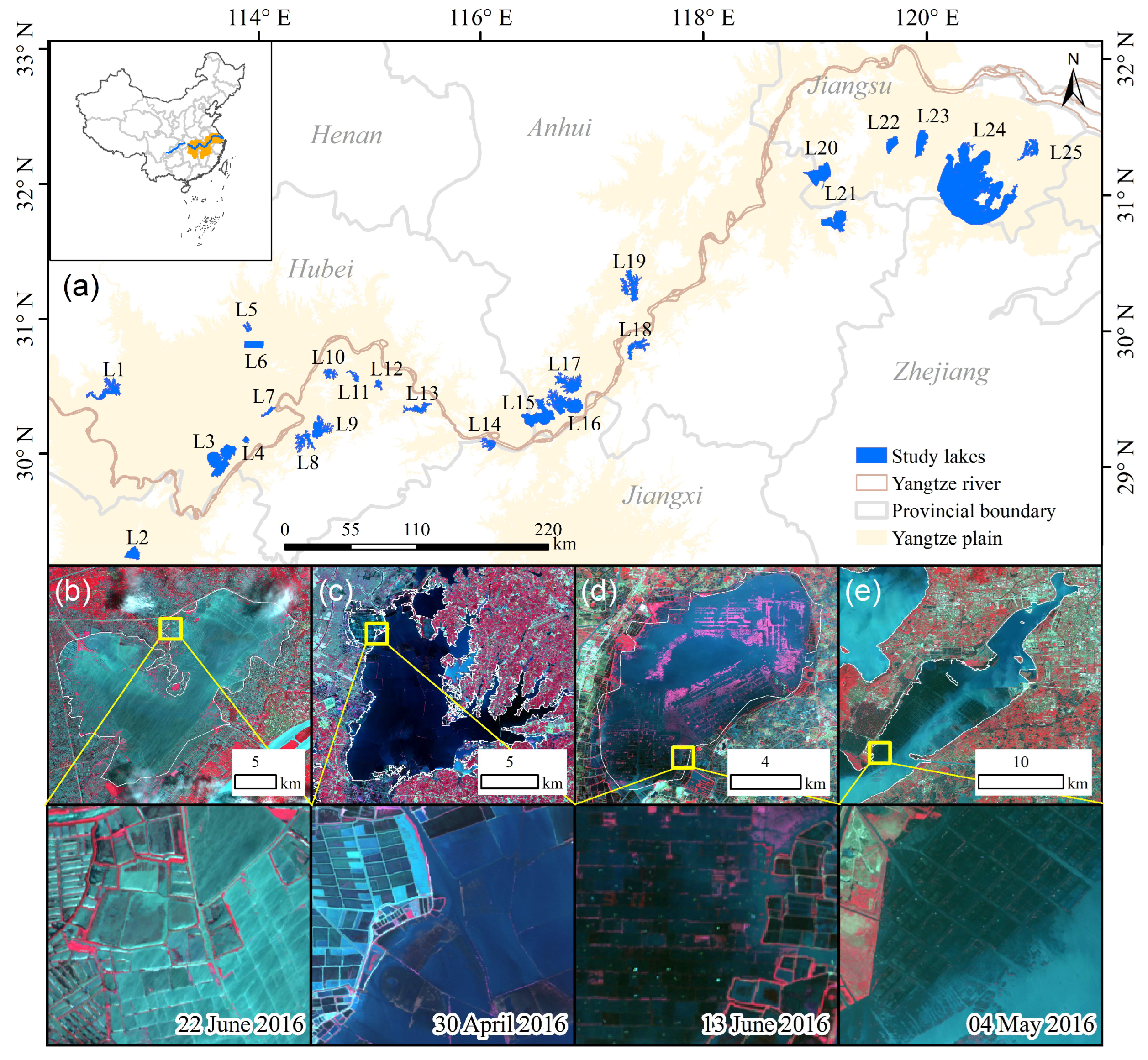
This study selected the MLRYR basin (28°30′–32°20′N, 114°30′–121°00′E) as the research area, encompassing provinces such as Hubei, Jiangsu, and Anhui. Lakes in this region are predominantly shallow and river-connected (average depth < 5 m), and most have historically supported EA activities [27,43]. Under the “Yangtze River’s Great Protection Strategy” strategy, extensive environmental management measures, including EA demolition, have been widely implemented. This study focuses on 25 lakes larger than 10 km2 within this region with documented EA records [27], to conduct long-term monitoring of EA and AV (Figure 1).

2.2. Data Sources

Remote sensing data collection and processing were conducted on the Google Earth Engine (GEE) platform. Landsat series imagery (Landsat 5 TM and Landsat 8 OLI) at 30 m resolution was selected for AV extraction, while Sentinel-1 SAR data at 10 m resolution was used for EA monitoring. Landsat 5 TM data (Dataset ID: LANDSAT/LT05/C02/T1_L2) from 1989 to 2011 and Landsat 8 OLI data (Dataset ID: LANDSAT/LC08/C02/T1_L2) from 2013 to 2023, with a 16-day revisit cycle, were utilized. Landsat imagery preprocessing on GEE included: ① cloud masking using the QA_PIXEL band, strict selection of high-quality images with <20% cloud cover, ② restriction of the image time range to the main AV growing season (April–October) [44], and ③ clipping using lake boundary vectors [45] to generate an image dataset from 1989 to 2023 for subsequent AV extraction and monitoring. Sentinel-1 data were sourced from the European Space Agency’s Copernicus program. The Sentinel-1A/1B constellation, equipped with C-band SAR, achieves a revisit cycle of up to 6 days. Based on the GEE platform, Sentinel-1 IW GRD data (Dataset ID: COPERNICUS/S1_GRD) from 2016 to 2023 were selected and clipped using lake boundaries to obtain SAR imagery for subsequent net-pen monitoring.

2.3. EA Mapping

This study employed the automated EA extraction algorithm proposed by Huang et al. (2025) to generate a long-term time-series dataset for analyzing spatiotemporal changes in the EA extent within the studied lakes [27]. The algorithm, implemented using a U-Net model, obtains EA data through three main steps: ① data preprocessing, ② model construction and training, and ③ post-processing (Figure S1).
First, Sentinel-1 SAR imagery was preprocessed by applying temporal median compositing to reduce noise. To enhance the textural separability between EA and open water, the V V m V H index (Equations (1) and (2)) was calculated [8].
V V m V H = V V m e d i a n × V H m e d i a n
w h e r e   V V m e d i a n and V H m e d i a n represent the median values of time series for VV and VH polarizations, respectively. The median backscatter coefficient for each pixel ( x , y )   was obtained as
m e d i a n σ x , y = m e d i a n { σ ( x , y ) , 1 , σ ( x , y ) , 2 , σ ( x , y ) , 3 σ ( x , y ) , n }
where σ ( x , y ) , n donates the pixel backscattering coefficient for the n-th scene at location ( x , y ) .
Second, a pixel-level binary reference mask was created through visual interpretation and labeling of the EA area. The training dataset was augmented through horizontal, vertical, and diagonal rotations, resulting in paired SAR images and corresponding binary labels. A U-Net model, following the architecture proposed by Ronneberger et al. [46], was employed for EA extraction. The model consists of two key stages: the encoding phase and the decoding phase (see Figure S1). The model consists of an encoder–decoder structure with skip connections (Figure S1). The encoder comprises four modules, each containing two convolutional layers followed by a max-pooling layer, progressively increasing the number of feature channels. The decoder similarly contains four modules, each with two convolutional layers, where feature maps from the encoder are concatenated via skip connections before up sampling via transposed convolution. Detailed training hyperparameters are provided in Table S1.
Subsequently, post-processing included a sliding-window approach to suppress noise and morphological operations to reconnect fragmented EA regions. The resulting binary EA maps were vectorized to compute total EA area and length per lake.
The extraction accuracy was evaluated against visually interpreted reference data using Intersection over Union (IoU), Frequency-Weighted IoU (FWIoU), and Overall Pixel Accuracy (OPA). The method demonstrated high agreement with validation samples, with OPA > 80% and IoU > 70%. Specific performance metrics for studied lakes, such as Lake Honghu (OPA = 0.82, IoU = 0.79, FWIoU = 0.64), Lake Futou (OPA = 0.86, IoU = 0.76, FWIoU = 0.71), and Lake Yangcheng (OPA = 0.91, IoU = 0.80, FWIoU = 0.71) (Figure S2), confirmed the robustness of the approach across different water bodies.

2.4. AV Communities Mapping

The VBI algorithm proposed by Luo et al. (2023) was employed to classify Landsat imagery [36], categorizing each pixel into one of four classes: AB, open water (OW), FEAV, and SAV. The entire process was implemented on the GEE platform. The classification involves three sequential steps. Step 1: The AVI, constructed from the wetness component of the Tasseled Cap Transformation, was utilized to distinguish AV from non-AV areas. Owing to the high sensitivity of AVI to complex lake optical characteristics, a linear mixture model was applied to derive dynamic thresholds for AVI. Step 2: Within the identified AV areas, NDVI was used to differentiate between FEAV and SAV. Pixels where NDVI was exceeding a specified threshold (TNDVI) were classified as FEAV, while the remaining areas were designated as SAV. Step 3: In non-AV areas, FAI was applied to discriminate AB from water. Pixels with FAI surpassed a defined threshold (TFAI) were identified as AB. Thresholds TFAI and TNDVI were determined based on histogram statistics of the maximum gradient of selected imagery. A universal FAI threshold for large-scale and long-term time-series analysis was obtained by subtracting twice the standard deviation from the mean of the FAI threshold histogram statistics. As NDVI and FAI thresholds followed a normal distribution, thresholds were set as TNDVI = 0.20 and TFAI = 0.02, consistent with Luo et al. (2023) [36]. Spatial distribution maps of different AV groups were generated. The annual maximum vegetation coverage, defined as the vegetation area divided by the lake area, was calculated to build a long-term AV time-series dataset.
The VBI algorithm has proven effective in eutrophic lakes of the MLRYR basin, achieving an overall classification accuracy of 84.5% [36]. In this study, validation was performed using a combined dataset of field surveys and visual interpretation (Table S2). Classification accuracies for Lake Taihu, Lake Changdang, Lake Nanyi, and Lake Datong resulted in an overall accuracy of 85.9% (Table S3, Figure S3), confirming the robustness of the method in the studied lakes.

2.5. Data Analysis

To elucidate long-term ecological changes in the lakes, the acquired time-series datasets (EA data from 2016 to 2023 and AV data from 1989 to 2023) were integrated and analyzed. For EA analysis, annual area, total length, coverage (EA area/lake area), and density (length/area) were calculated for each lake. The maximum EA area during the monitoring period and its corresponding year were identified. The year of complete EA removal was defined as when the EA coverage fell below 5%. To quantify heterogeneity in removal progress, lakes exhibiting either an 80% or greater reduction in EA coverage over two consecutive years or a direct decline to below 5% coverage were categorized as “lakes with rapid EA reduction.” For AV data, annual area and coverage of FEAV and SAV were extracted. Generalized Additive Models (GAMs) were employed to fit long-term trends for each vegetation type [47]. Trends were categorized into five types: Decrease, Unimodal, Increase, Recovery, and Insignificant, following the classification scheme of Botrel & Maranger (2023) [48]. The “Insignificant” category included lakes with no statistically significant trend, stable vegetation, or substantial fluctuations without a clear directional trend. Analyses were conducted at two scales: independent trend analysis for each vegetation group within each lake, and aggregated trend analysis using vegetation data from all enclosure lakes. Additionally, to examine spatial dynamics of macrophytes at a fine scale, we computed the annual frequency of SAV occurrence (F) at the pixel level for the growing season (April–October) from 2017 to 2023. This frequency was defined as the number of times a pixel was classified as SAV divided by the total number of valid observations for that pixel in a given year. Apart from the calculation of SAV frequency at the pixel scale, which is performed in the Python 3.11.5 environment, all other data preprocessing and statistical analyses were conducted in the R 4.5.0 environment.

3. Results

3.1. Changes in EA

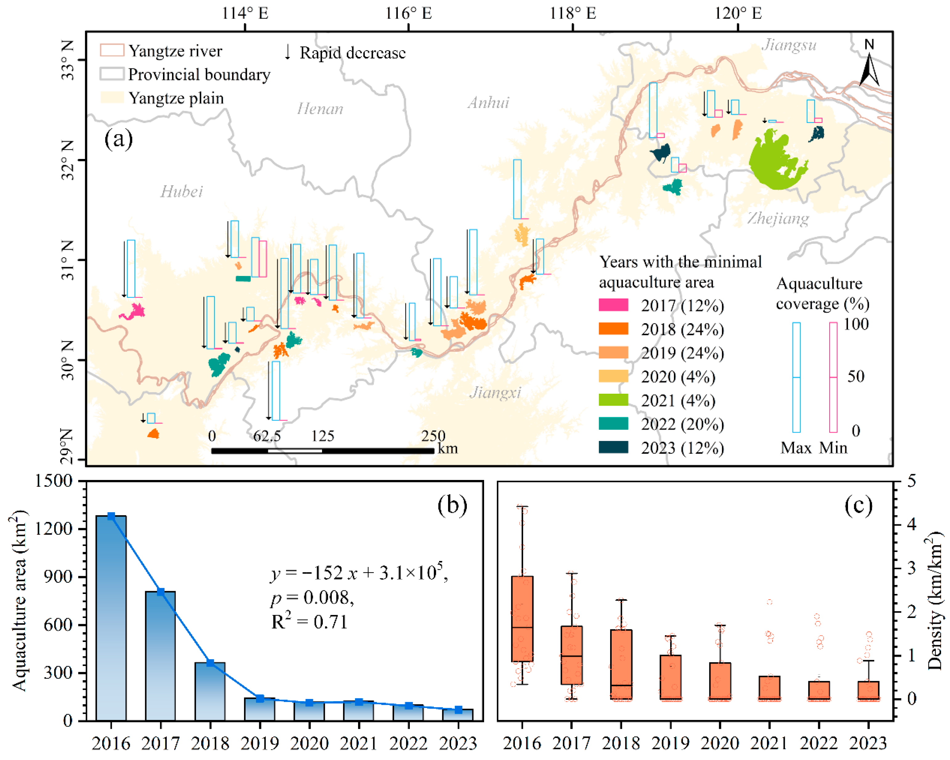
Monitoring data from 2016 to 2023 for lakes >10 km2 in the MLRYR basin revealed dramatic changes in EA patterns over this eight-year period (Figure 2). Overall, the total EA area in regional lakes sharply decreased from 1280.5 km2 in 2016 to 71.0 km2 in 2023, representing a relative reduction of 94.5% (p = 0.008, R2 = 0.71). Temporally, the removal process exhibited distinct phases: the period from 2017 to 2019 was characterized by a rapid removal phase, marking the peak of EA demolition, during which the EA area decreased at an average annual rate of 51%. After 2019, the EA reduction rate slowed noticeably, with the average annual decrease dropping to 15% (Figure 2b).
At the individual lake level, 48% of lakes reached their minimum EA area in either 2018 or 2019 (Figure 2a). Correspondingly, the median EA density across all lakes significantly decreased from 1.6 km/km2 in 2016 to 0.3 km/km2 in 2018, and further dropped to 0 by 2019 (Figure 2c). Regarding removal progress, by 2019, 72% of lakes (n = 18) had essentially completed EA removal (coverage ratio < 5%); this proportion increased to 88% by 2023. Currently, only three lakes—Lake Diaocha, Nanyi, and Changdang—still exhibited significant EA activity (remaining EA coverage ratio > 5%). Among lakes where removal was completed, 80% were categorized as “lakes with rapid EA reduction”, predominantly located in the MLRYR basin. In terms of absolute EA removal magnitude, the top five lakes with the largest reduction percentages were Lake Futou (64.6%), Lake Longgan (61.9%), Lake Bo (60.1%), Lake Daye (59.6%), and Lake Caizi (54.5%).

3.2. Long-Term Dynamics of AV

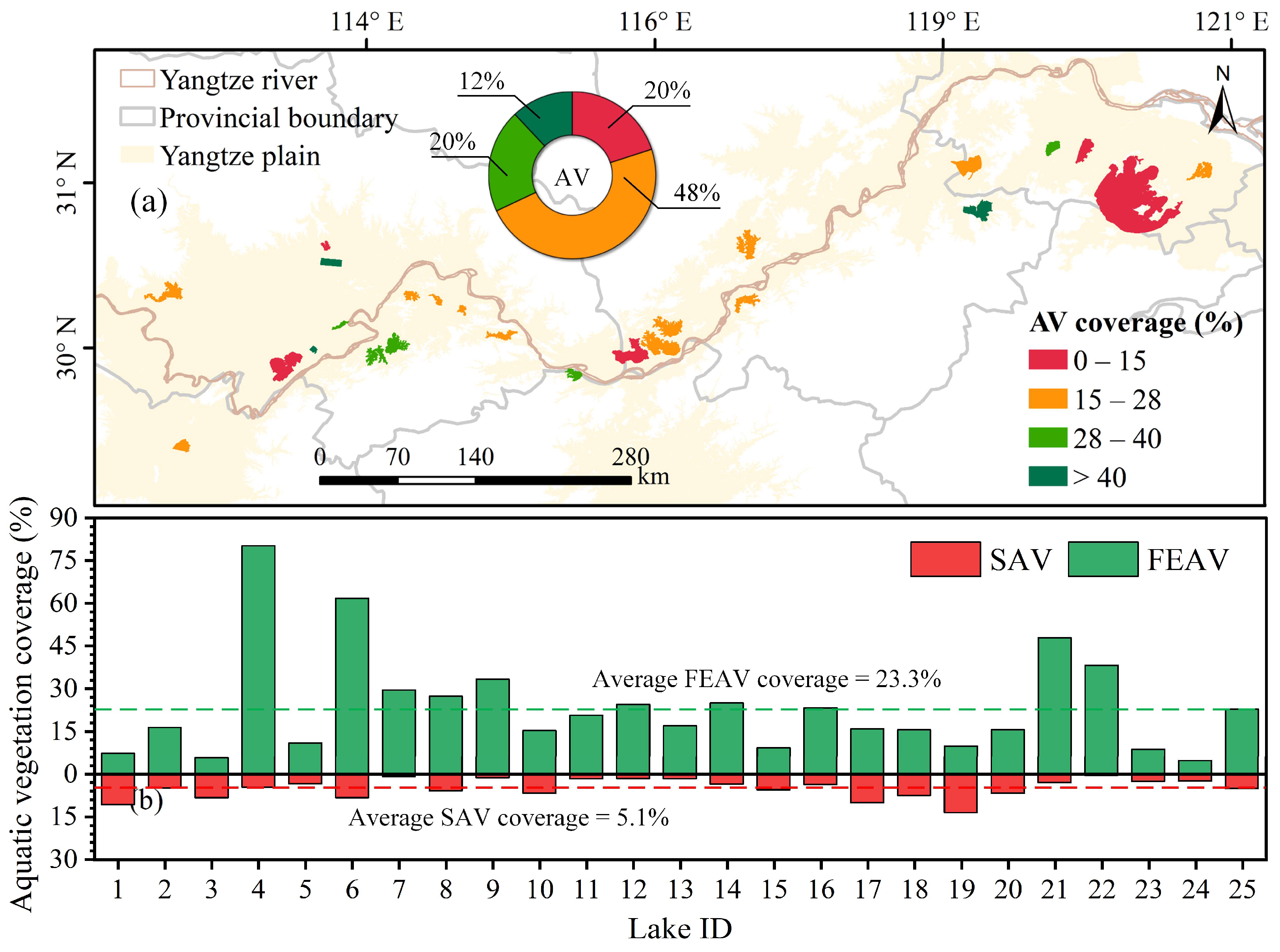
In 2023, the total AV area in the studied lakes was 953.5 km2, accounting for 17.4% of the total lake area. Regarding group composition, FEAV was the dominant group, constituting 74.1% of the total vegetation area, while SAV accounted for only 25.9%. At the individual-lake level, the mean AV coverage was 28.5%. The majority of lakes (68%) exhibited vegetation coverage below this mean. Specifically, the coverages in Lake Longgan (C = 14.8%), Lake Dongxicha (C = 14.3%), Lake Honghu (C = 14.0%), Lake Gehu (C = 11.2%), and Lake Taihu (C = 7.2%) were all below 15%. Eight lakes, including Lake Lihu (C = 84.9%), Lake Diaocha (C = 70.2%), Lake Nanyi (C = 51.0%), Lake Changdang (C = 38.8%), Lake Futou (C = 34.7%), Lake Xiliang (C = 33.2%), Lake Wuhu (C = 30.4%), and Lake Chihu (C = 28.6%) had coverage levels exceeding the mean (Figure 3a). FEAV was generally the dominant group in the study lakes. The mean coverage of FEAV and SAV was 23.3% and 5.1%, respectively (Figure 3b). In 22 lakes (88%), the FEAV coverage exceeded the SAV coverage. Notably, in the aforementioned eight lakes with high overall coverage, FEAV contributed over 80% of the total.
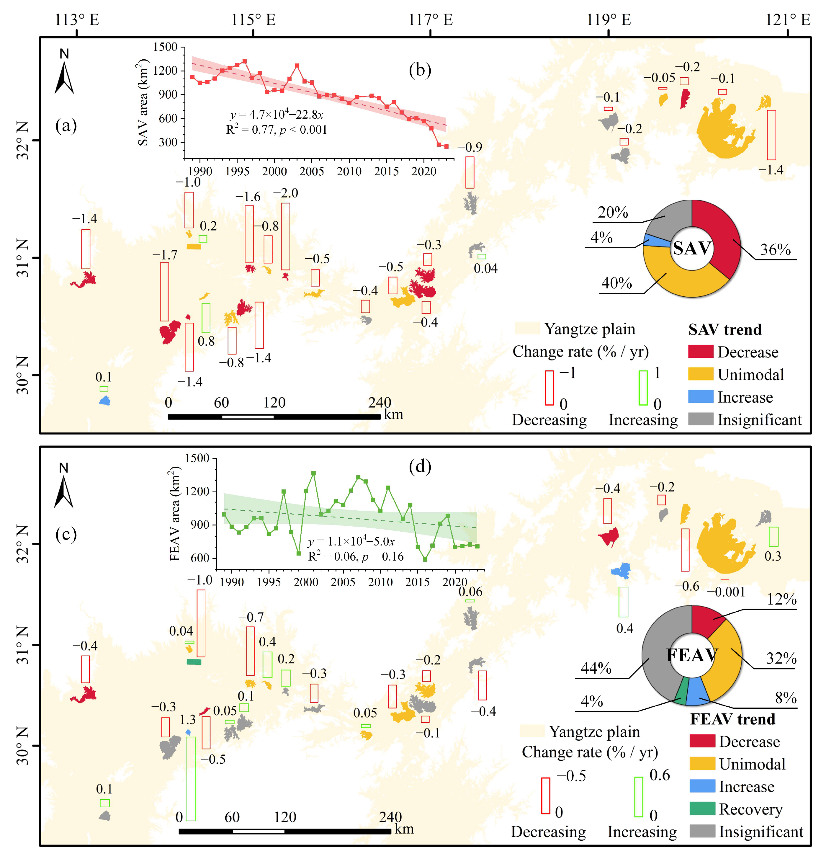
Between 1989 and 2023, AV in the study lakes underwent dramatic spatiotemporal evolution, with SAV and FEAV exhibiting distinctly different patterns of change (Figure 4). At the regional scale, SAV area showed a significant decreasing trend (R2 = 0.77, p < 0.001), declining continuously from 1120.9 km2 in 1989 to 247.3 km2 in 2023, with an accelerated decrease rate after 2016 (Figure 4b). In contrast, the FEAV area did not exhibit a significant trend (R2 = 0.06, p = 0.16). Its mean values for different periods were 899.1 km2 before 2000, 1160.6 km2 during the 2000s, and 834.4 km2 after 2010 (Figure 4d). Overall, total AV area decreased by 55.0% over the 34-year period, from 2116.8 km2 to 953.5 km2. Analyzing change types at the individual-lake level, primary trends for SAV were “Decrease” (36% of lakes) and “Unimodal” (increase followed by decrease, 40%). Changes were “Insignificant” in 28% of the lakes, and only Lake Datong exhibited an “Increase” trend. For FEAV, the “Unimodal” trend was the most common (32% of lakes), followed by “Decrease” (12%) and “Increase” (8%), while changes were “Insignificant” in 44% of the lakes (Figure 4c). Regarding change rates, the vast majority of lakes (84%) experienced a decline in SAV coverage, with Lake Honghu, Lake Tangxun, and Lake Sanshan showing the highest decline rates. Concurrently, over half of the lakes (56%) also experienced a decrease in FEAV coverage, with Lake Diaocha, Lake Tangxun, and Lake Gehu exhibiting the highest decline rates. In summary, large-scale and rapid SAV decline was the dominant driver behind the decrease in total AV area, indicating widespread vegetation degradation in MLRYR basin enclosure lakes since approximately 2010.

3.3. Changes in SAV After EA Demolition

The observed decline in SAV was particularly concerning due to its critical ecological role. SAV is highly sensitive to changes in hydrodynamic conditions and light availability, making it an excellent indicator of ecosystem health [49,50,51]. Understanding the specific impacts of EA removal on this sensitive vegetation is crucial for effective lake management and restoration efforts. Given the ecological significance and observed sensitivity of SAV, this section specifically examines its response to the extensive EA removal efforts in the MLRYR basin.
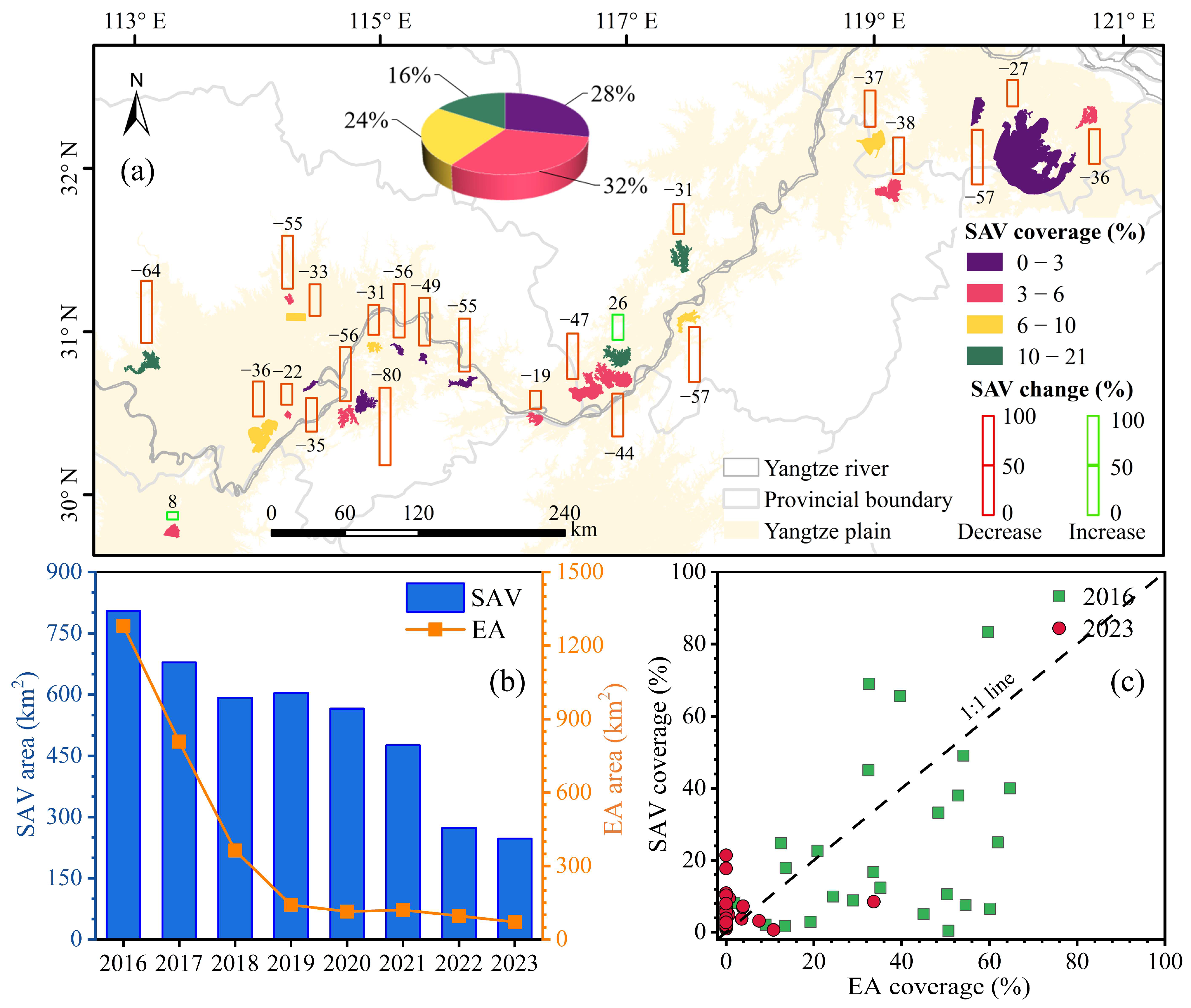
Despite varying EA removal progress across lakes, AV, particularly the environmentally sensitive SAV, generally exhibited a significant declining trend (Figure 4 and Figure 5). Currently, SAV coverage in the enclosure lakes of MLRYR is low, with a mean value of only 5.1%, and over half (52%) of lakes fall below this average (Figure 5a). Between 2016 and 2023, while total EA area decreased by 31.6%, SAV area declined sharply from 804.8 km2 to 247.3 km2, representing a substantial reduction of 69.3% (Figure 5b). Among the 25 enclosure lakes, only Lake Bohu and Lake Datong showed an increasing trend in SAV coverage across the two observation periods (2016–2019 and 2020–2023). The remaining 23 lakes displayed declining trends, with Lake Futou, Lake Changhu, Lake Shengjin, Lake Gehu, and Lake Changdang experiencing the most severe degradation (Figure 5a). Scatter plot analysis of the relationship between SAV coverage and EA area ratio further revealed a close association between the two variables (Figure 5c). In 2016, data points for the lakes were relatively dispersed, showing occurrences of either a high SAV coverage or a high EA ratio. By 2023, however, data points clustered within the range where both the SAV coverage and EA extent were below 20%, corroborating an intrinsic link between the presence of EA and the abundance of SAV (Figure 5c).
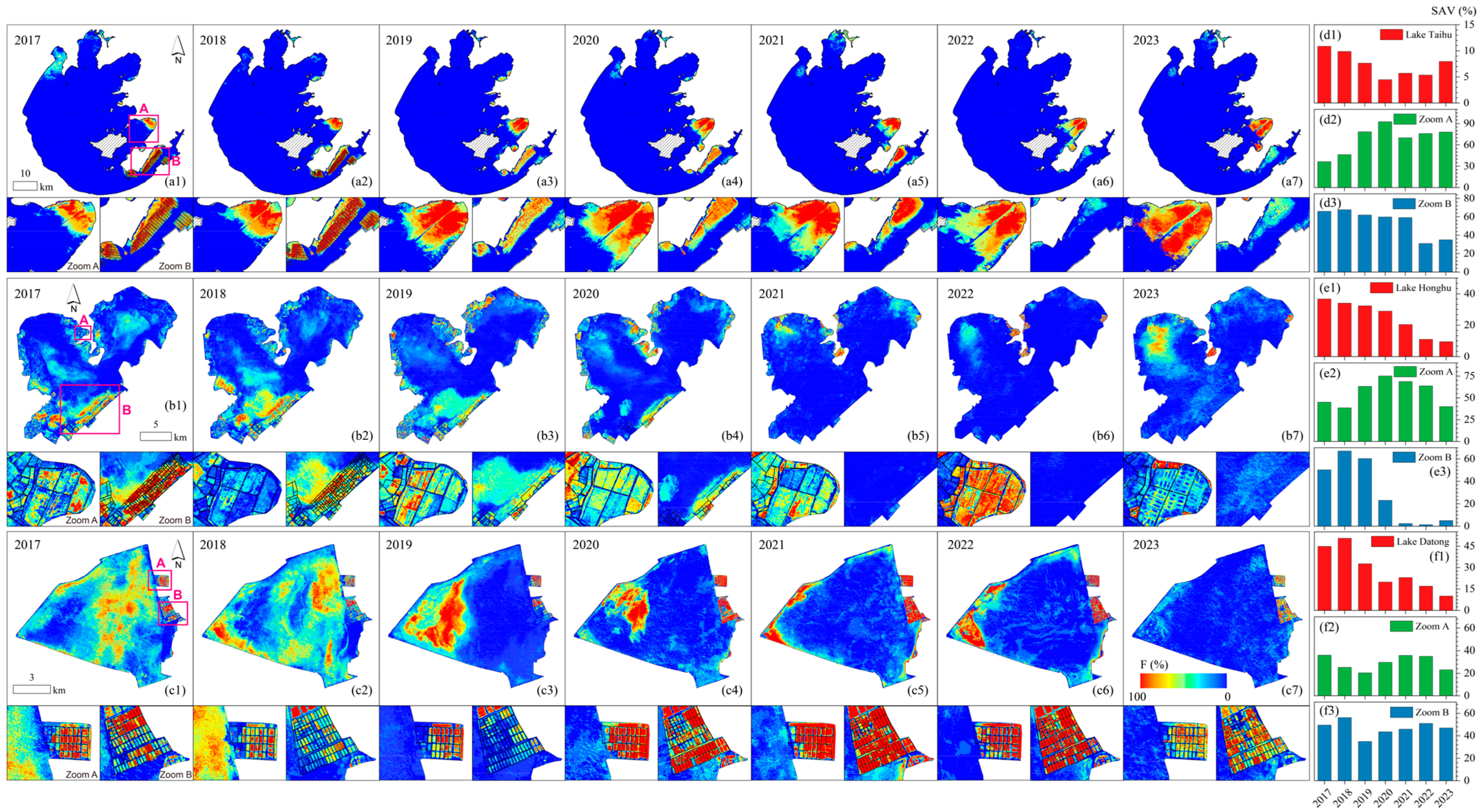
To further investigate the direct impact of EA removal on SAV, this study selected Lake Taihu, Lake Honghu, and Lake Datong as representative case studies. The analysis focused on EA areas, areas where nets were removed, and non-EA areas to examine the spatiotemporal dynamics of SAV from 2017 to 2023 (Figure 6). The results indicate that (1) Rapid vegetation degradation occurred in EA removal areas; before removal, SAV within EA areas was densely distributed and exhibited high coverage (Figure 6(a1–c1)). Following removal, vegetation in these former EA areas significantly decreased or even disappeared (Figure 6(a2–a7)). This process was particularly evident in areas undergoing gradual removal, such as Zoom B in Lake Honghu, where vegetation declined synchronously with the progressive dismantling of nets and nearly vanished after complete removal in 2021 (Figure 6(b5)). (2) Relatively stable vegetation growth persisted in remaining EA areas: In areas where EA continued to exist and SAV coverage showed minor fluctuations (e.g., Figure 6(f2,f3)) and remained densely distributed within the EA boundaries. For instance, SAV thrived within the two EA areas of Lake Datong throughout the observation period (Figure 6(c5,c6)). (3) Complex vegetation dynamics characterized non-EA areas: SAV dynamics in non-EA areas exhibited spatial heterogeneity, with an overall increasing yet unstable trend. For example, SAV in Zoom A of Lake Taihu became increasingly dense (Figure 6(a1–a7)), with coverage significantly increasing from 36% in 2017 to 78% in 2023 (Figure 6(d2)). Conversely, in the western part of Lake Datong, extensive SAV observed in 2019 had nearly disappeared by 2023, indicating distribution instability (Figure 6(c3–c7)).
In summary, EA removal was a significant factor contributing to the marked decline of SAV, which was particularly evident in the near-complete loss of vegetation in removal areas. In contrast, the continued EA presence provided a relatively stable growth environment for SAV.

4. Discussion

4.1. Why Does AV Loss Occur After EA Removal?

Aquaculture is widely recognized as a key driver of lake eutrophication [10], prompting large-scale EA demolition in the MLRYR basin to reduce nutrient loads. However, monitoring results indicated a concomitant sharp decline or even disappearance of AV, primarily SAV, following EA removal (Figure 5 and Figure 6). This finding does not suggest that the ecological restoration measure (i.e., EA demolition) was misguided, but rather highlights the dual ecological role of EA in lake ecosystem management.
AV, especially SAV, constitutes an important component of the aquaculture system, reflecting the integral ecological role of EA. Within EA areas, AV served not only as ideal feed for fish and crabs but also functions in wastewater treatment, water-quality improvement, and enhancing water productivity [52]. Under this integrated “aquaculture–AV” symbiosis model, lush vegetation is directly linked to higher yields and economic benefits, which incentivizes fishermen to autonomously manage SAV, including harvesting FEAV and planting SAV. As observed in Lake Datong, SAV showed a fluctuating but increasing trend from 2017 to 2023 within areas where some net pens remained (Figure 6(c1–c7)). Although large-scale artificial vegetation restoration was also implemented in this lake [53], consistent and targeted management by fishermen within the EA areas undoubtedly served as a crucial synergistic factor enabling vegetation maintenance and growth amidst the widespread decline of AV in the MLRYR basin [54].
However, after EA removal, fishermen naturally ceased vegetation management, inevitably impacting the growth of AV [5]. Concurrently, a cascade of physical and chemical environmental changes further exacerbated vegetation degradation. Physically, the loss of EA structures increased hydrodynamic forces in previously occupied areas. Artificial structures within aquaculture zones, such as net pens, can act to dampen wave action and reduce water turbulence [55]. Their removal consequently increases sediment resuspension and light attenuation in the water column [12], creating an unfavorable environment for light-dependent SAV [13]. This heightened disturbance can suddenly uproot and kill SAV with low wave-resistance, while potentially creating expansion conditions for more robust FEAV [5,56]. Chemically, EA areas, affected by years of feed input and fertilization, exhibit high nutrient-loads, low water-transparency, and insufficient underwater light, collectively forming a stressful environment unsuitable for the germination and growth of SAV [53,57]. This also explains why, even during the EA period, vegetation communities were often dominated by pioneer species with high pollution-tolerance and low light-requirements, such as Potamogeton crispus and Myriophyllum spicatum [5,7].

4.2. What Are the Consequences of AV Degradation?

Having established the likely drivers of AV degradation following EA removal, it is crucial to consider the potential ecological consequences of this vegetation loss. AV plays multiple roles in maintaining ecosystem health as a key primary producer in lakes. It directly improves water quality by absorbing nutrients such as nitrogen and phosphorus [50], and stabilizes sediments through root systems, thereby reducing wind–wave disturbance, preventing shoreline erosion, and minimizing sediment resuspension [58]. It is vital for sustainable lake-ecosystem development [59]. Once vegetation undergoes large-scale degradation, these ecological functions are lost, triggering cascading reactions. Reduced vegetation-cover intensifies wind–wave disturbance and increases water-flow velocity, causing sediment resuspension [60]—a primary source of internal nutrient loading in eutrophic lakes [61]. Concurrently, increased suspended solid concentrations significantly reduces water transparency, further inhibiting SAV photosynthesis [62]. The initial decline in vegetation marks the onset of a positive feedback mechanism, driven by increased turbidity and compromised light penetration, which perpetuates and intensifies the degradation process. Research on AV in East Lake Taihu confirmed this, demonstrating that SAV and FEAV changes were closely related to wind speed and water transparency, with a significant positive correlation between AV coverage and transparency [6,56].
Within the aquatic ecosystem food web, AV provides food for fish and peripheral birds, and offers attachment substrates and habitats for microorganisms [63]. Its degradation inevitably leads to biodiversity loss. The historical ecological changes in Lake Honghu served as evidence: since the 1960s, under the influence of extensive human activities (including water regulation, flood discharge, net-pen aquaculture, and fishing), the water-quality of Lake Honghu noticeably deteriorated, and AV coverage decreased by over 60%. This was followed by a sharp decline in fish species richness and species composition homogenization [64], illustrating cascading negative impacts of vegetation degradation on aquatic communities. Furthermore, vegetation degradation also drives the homogenization of the vegetation community structure itself. Under environmental stress, more vulnerable species gradually disappear, and community composition degrades to dominance by pollution-tolerant species like Potamogeton crispus, Myriophyllum spicatum, and Ceratophyllum demersum, along with floating-leaved vegetation [65]. This trend towards community homogenization significantly weakens ecosystem resistance and resilience to external disturbances, leading to declined overall stability [66,67].
More critically, SAV decline can drive a regime shift from a macrophyte-dominated clear-water state to a phytoplankton-dominated turbid-water state. Following SAV degradation, its inhibitory effect on algae diminishes. Nitrogen and phosphorus nutrients are then absorbed by phytoplankton, increasing cyanobacteria dominance and making cyanobacterial blooms more likely to happen [65,67]. This risk is amplified in already eutrophic EA lakes. For instance, in East Lake Taihu, after EA removal and a sharp decline of SAV (Figure 6(a1–a7)), an algal bloom covering 8.79 km2 rapidly occurred in the Taipu Gate area, which had not experienced blooms before [5]. Similarly, in Lake Changdang, following EA removal and a rapid decrease in SAV (Figure 5a), large-scale AB occurred consecutively in 2020 and 2021 [68,69]. These cases indicated that the loss of SAV dominance often signified that the lake was likely undergoing a regime shift from a clear-water state to a turbid-water state dominated by phytoplankton [70,71]. This led to impaired lake-ecosystem services and decreased ecosystem resilience, and makes ecological restoration exceptionally difficult.

4.3. How Can Vegetation Loss Be Effectively Addressed in Lake Restoration?

Given the severe consequences outlined above, effective strategies to mitigate vegetation loss and promote lake restoration are urgently needed. Indeed, the action of returning nets to the lake has demonstrated significant effectiveness in improving lake water-quality [4,72], which is crucial for the long-term health of the lake ecosystems in the Yangtze River basin. However, the short-term AV degradation, particularly SAV, revealed by this study, underscores the complexity and challenges inherent in the ecological restoration of eutrophic lakes [73]. This phenomenon also reflects the hysteresis effect in lake ecosystems [63,70], whereby the recovery of ecological state often lags behind the improvement of water-quality parameters. This implies that nutrient loads must be reduced to levels far below the critical threshold that initially triggered degradation for the ecosystem to potentially cross the threshold and return to a clear-water state [74]. Consequently, future lake management must transition from a singular focus on water-quality targets towards a systematic and long-term ecological restoration framework.
In the short-term, combining artificial interventions for nutrient control in lakes is necessary. Existing research indicates that controlling external nutrient inputs and blocking internal nutrient release are crucial measures for addressing lake eutrophication and cyanobacterial blooms [75,76]. For water bodies that remain highly nutrient-enriched following EA removal, continuous control of external pollution is required [75]. Engineering measures such as constructing ecological floating islands and lakeside buffer zones should be implemented to reduce point and non-point source pollution entering the lakes. Secondly, targeted internal pollution control should be carried out. Depending on the sedimentation status and ecological conditions of the lake, methods such as sediment remediation or dredging should be employed to reduce the concentrated nutrients in the sediment, thereby creating suitable habitat conditions for aquatic organisms [77,78]. In the long-term, proactive adoption of biomanipulation methods is recommended. This involves regulating the fish community structure [79] to increase the population of large herbivorous zooplankton, supplemented by artificial planting and maintenance, to re-establish the dominant community of submerged macrophytes, thereby suppressing AB [68,80,81]. At the watershed scale, lake shoreline restoration is necessary, reconnecting water channels blocked by dams and restoring hydrological connectivity [72]. Furthermore, for precise implementation, remote-sensing technology should be fully utilized to construct an integrated sky–air–ground monitoring network. By collaboratively inverting key parameters such as AV coverage and water nutrient status using multi-source remote sensing data [42,82,83], dynamic diagnosis of ecological restoration progress and early risk warning can be achieved. This represents a potential pathway towards intelligent watershed management.

5. Conclusions

This study integrated Landsat and Sentinel-1 series imagery to construct datasets of EA and AV, analyzing ecological impacts of action of returning nets to the lake on EA lakes in the MLRYR. Results demonstrated that from 1989 to 2023, the SAV area in the 25 studied EA lakes decreased significantly, while FEAV area exhibited fluctuating trends. Particularly following EA removal (2016–2023), vegetation nearly vanished in former EA areas, whereas it remained relatively stable in areas where nets were retained. The SAV area declined rapidly by 53.2% during this period. This indicated that the action of returning nets to the lake was a significant contributing factor to short-term degradation of the SAV. Ongoing degradation of AV can lead to imbalances in lake ecological structure and function, potentially driving a regime shift from a macrophyte-dominated clear-water state to a phytoplankton-dominated turbid-water state. Currently, while demolition of EA had achieved remarkable success in improving water-quality, the ecological restoration exhibited significant hysteresis. Future lake ecological restoration efforts should adopt integrated management strategies that balance water quality improvement with active ecological rehabilitation. This involves continuously advancing pollution control and nutrient load reduction while prioritizing ecological engineering focused on AV restoration, supplemented by biological regulation methods, such as biomanipulation. These integrated approaches are essential for comprehensively enhancing the resilience and long-term sustainability of lake ecosystems.

Supplementary Materials

The following supporting information can be downloaded at: https://www.mdpi.com/article/10.3390/rs18030400/s1, Figure S1: Technical flowchart of the lake enclosure aquaculture (EA) extraction algorithm; Figure S2: Validation of EA extraction results. a-f: corresponding VH/VV images of the lakes; a1–f1: extracted EA results overlaid with labels, where red lines represent labels and blue lines represent extraction results; Figure S3: False color images and classification maps derived by VBI algorithm in Lake Taihu, Lake Changdang, Lake Nanyi and Lake Datong. Different colors in classification maps represent different groups, including open water (OW), FEAV, SAV, and AB; Table S1: Model training parameters for EA extraction; Table S2: Investigation details of AV and AB in lakes, and the time of image acquisition. Field surveys for on-site sampling were conducted to ensure the reliability of ground sample points for validating satellite monitoring results. During sampling, the coverage and dominant vegetation types of AV within the range of two pixels (60 m × 60 m) were visually estimated. Visual interpretation combined with JL-1 high-resolution imagery (0.7 m), selecting points in the lake for validation; Table S3: Confusion matrix between measured class and mapped class derived from the VBI algorithm.

Author Contributions

Y.X., conceptualization, methodology, data analyses, and writing; S.X. and J.L., methodology, supervision, and funding acquisition; G.C., data curation and analyses. All authors have read and agreed to the published version of the manuscript.

Funding

This study was financially supported by the National Natural Science Foundation of China (42271377) and by Key Laboratory of Lake and Watershed Science for Water Security (NKL2023-KP02).

Data Availability Statement

The satellite imagery used in this paper were obtained through Google Earth Engine platform.

Conflicts of Interest

The authors declare no conflicts of interest.

References

  1. Dong, S.-L.; Cao, L.; Liu, W.-J.; Huang, M.; Sun, Y.-X.; Zhang, Y.-Y.; Yu, S.-E.; Zhou, Y.-G.; Li, L.; Dong, Y.-W. System-Specific Aquaculture Annual Growth Rates Can Mitigate the Trilemma of Production, Pollution and Carbon Dioxide Emissions in China. Nat. Food 2025, 6, 365–374. [Google Scholar] [CrossRef]
  2. Naylor, R.L.; Goldburg, R.J.; Primavera, J.H.; Kautsky, N.; Beveridge, M.C.M.; Clay, J.; Folke, C.; Lubchenco, J.; Mooney, H.; Troell, M. Effect of Aquaculture on World Fish Supplies. Nature 2000, 405, 1017–1024. [Google Scholar] [CrossRef]
  3. Naylor, R.L.; Hardy, R.W.; Buschmann, A.H.; Bush, S.R.; Cao, L.; Klinger, D.H.; Little, D.C.; Lubchenco, J.; Shumway, S.E.; Troell, M. A 20-Year Retrospective Review of Global Aquaculture. Nature 2021, 591, 551–563. [Google Scholar] [CrossRef] [PubMed]
  4. Yu, H.; Wang, Z.; Wang, H.; Liang, Y.; Li, X. Lake demolition monitoring and estimation of ecological environment benefits in Jianghan Plain: A case study of the Honghu Lake. Resour. Environ. Yangtze Basin 2020, 29, 2760–2769. [Google Scholar]
  5. Yang, J.; Luo, J.; Lu, L.; Sun, Z.; Cao, Z.; Zeng, Q.; Mao, Z. Changes in aquatic vegetation communities based on satellite images before and after pen aquaculture removal in East Lake Taihu. J. Lake Sci. 2021, 33, 507–517. [Google Scholar] [CrossRef]
  6. Luo, J.; Pu, R.; Ma, R.; Wang, X.; Lai, X.; Mao, Z.; Zhang, L.; Peng, Z.; Sun, Z. Mapping Long-Term Spatiotemporal Dynamics of Pen Aquaculture in a Shallow Lake: Less Aquaculture Coming along Better Water Quality. Remote Sens. 2020, 12, 1866. [Google Scholar] [CrossRef]
  7. Xu, J.; Zhong, W.; Cai, Y.; Gong, Z.; Wen, X. Trend of Water Environment Change in Lake Changdang and Lake Gehu in the Last 30 Years. Resour. Environ. Yangtze Basin 2022, 31, 1641–1652. [Google Scholar]
  8. Sun, Z.; Luo, J.; Xu, Y.; Zhai, J.; Cao, Z.; Ma, J.; Qi, T.; Shen, M.; Gu, X.; Duan, H. Coordinated Dynamics of Aquaculture Ponds and Water Eutrophication Owing to Policy: A Case of Jiangsu Province, China. Sci. Total Environ. 2024, 927, 172194. [Google Scholar] [CrossRef]
  9. Liu, X.; Li, E.; Xu, J.; Deng, Z.; Huang, X.; Wang, Y.; Wang, X. Evolution mechanism of Lake Honghu wetland ecosystem and regime shift crucial threshold. J. Lake Sci. 2023, 35, 934–940. [Google Scholar] [CrossRef]
  10. Chen, J.; Liu, X.; Chen, J.; Jin, H.; Wang, T.; Zhu, W.; Li, L. Underestimated Nutrient from Aquaculture Ponds to Lake Eutrophication: A Case Study on Taihu Lake Basin. J. Hydrol. 2024, 630, 130749. [Google Scholar] [CrossRef]
  11. He, X.; Yan, W.; Chen, X.; Wang, Y.; Li, M.; Li, Q.; Yu, Z.; Wu, T.; Luan, C.; Shao, Y.; et al. Arsenic Distribution Characteristics and Release Mechanisms in Aquaculture Lake Sediments. J. Hazard. Mater. 2024, 476, 135141. [Google Scholar] [CrossRef]
  12. Farmaki, E.G.; Thomaidis, N.S.; Pasias, I.N.; Baulard, C.; Papaharisis, L.; Efstathiou, C.E. Environmental Impact of Intensive Aquaculture: Investigation on the Accumulation of Metals and Nutrients in Marine Sediments of Greece. Sci. Total Environ. 2014, 485–486, 554–562. [Google Scholar] [CrossRef]
  13. Qin, L.; Yang, J.; Ding, Z.; Shen, C. Aquaculture and Submerged Aquatic Vegetation as Key Drivers of Algal Blooms in Urban Lakes: Insights from Machine Learning Modeling. Ecol. Indic. 2025, 178, 114024. [Google Scholar] [CrossRef]
  14. Hu, M.; Ma, R.; Xiong, J.; Wang, M.; Cao, Z.; Xue, K. Eutrophication State in the Eastern China Based on Landsat 35-Year Observations. Remote Sens. Environ. 2022, 277, 113057. [Google Scholar] [CrossRef]
  15. Huang, J.; Zhang, Y.; Arhonditsis, G.B.; Gao, J.; Chen, Q.; Peng, J. The Magnitude and Drivers of Harmful Algal Blooms in China’s Lakes and Reservoirs: A National-Scale Characterization. Water Res. 2020, 181, 115902. [Google Scholar] [CrossRef]
  16. Ministry of Ecology and Environment of the People’s Republic of China. Guidelines for Water Ecological Assessment Indicators in Lakes. Available online: https://www.mee.gov.cn/xxgk2018/xxgk/xxgk05/202308/t20230824_1039240.html (accessed on 6 June 2023).
  17. Ministry of Ecology and Environment of the People’s Republic of China. Yangtze River Protection Law of the People’s Republic of China. Available online: https://www.mee.gov.cn/ywgz/fgbz/fl/202012/t20201227_814985.shtml (accessed on 26 October 2020).
  18. Ministry of Ecology and Environment of the People’s Republic of China. Opinions of the General Office of the CPC Central Committee and the General Office of the State Council on Comprehensively Promoting the River Chief System. Available online: https://www.mee.gov.cn/zcwj/zyygwj/201912/t20191225_751541.shtml (accessed on 11 December 2016).
  19. Xi Stresses High-Quality Development of Yangtze River Economic Belt. Available online: https://english.www.gov.cn/news/202310/13/content_WS652877c6c6d0868f4e8e029b.html (accessed on 13 October 2023).
  20. Lai, L.; Liu, Y.; Zhang, Y.; Cao, Z.; Yin, Y.; Chen, X.; Jin, J.; Wu, S. Long-Term Spatiotemporal Mapping in Lacustrine Environment by Remote Sensing: Review with Case Study, Challenges, and Future Directions. Water Res. 2024, 267, 122457. [Google Scholar] [CrossRef] [PubMed]
  21. Loewen, C.J.G. Lakes as Model Systems for Understanding Global Change. Nat. Clim. Change 2023, 13, 304–306. [Google Scholar] [CrossRef]
  22. Duan, H.; Cao, Z.; Shen, M.; Ma, J.; Qi, T. Review of lake remote sensing research. Natl. Remote Sens. Bull. 2022, 26, 3–18. [Google Scholar] [CrossRef]
  23. Wang, J.; Gao, J. Extraction of Enclosure Culture in Gehu Lake Based on Correspondence Analysis. Natl. Remote Sens. Bull. 2021, 12, 716–723. [Google Scholar] [CrossRef]
  24. Huang, S.; Song, K.; Luo, J. A remote sensing extraction algorithm of enclosure culture area in shallow lakes based on gradient transform. J. Lake Sci. 2016, 29, 490–497. [Google Scholar]
  25. Dai, Y.; Feng, L.; Hou, X.; Choi, C.-Y.; Liu, J.; Cai, X.; Shi, L.; Zhang, Y.; Gibson, L. Policy-Driven Changes in Enclosure Fisheries of Large Lakes in the Yangtze Plain: Evidence from Satellite Imagery. Sci. Total Environ. 2019, 688, 1286–1297. [Google Scholar] [CrossRef] [PubMed]
  26. Ottinger, M.; Clauss, K.; Kuenzer, C. Aquaculture: Relevance, Distribution, Impacts and Spatial Assessments—A Review. Ocean Coast. Manag. 2016, 119, 244–266. [Google Scholar] [CrossRef]
  27. Huang, L.; Zhai, J.; Sun, Z.; Xu, Y.; Gao, J.; Xin, Y.; Qin, H.; Zhao, J.; Ruan, C.; Xu, Y.; et al. Satellite remote sensing reveals substantial decrease of enclosure aquaculture in the Yangtze-Huaihe River Basin. J. Lake Sci. 2025, 37, 2260–2272. [Google Scholar] [CrossRef]
  28. Luo, J.; Yang, J.; Duan, H.; Lu, L.; Sun, Z.; Xin, Y. Research progress of aquatic vegetation remote sensing in shallow lakes. Natl. Remote Sens. Bull. 2022, 26, 68–76. [Google Scholar]
  29. Liang, Q.; Zhang, Y.; Ma, R.; Loiselle, S.; Li, J.; Hu, M. A MODIS-Based Novel Method to Distinguish Surface Cyanobacterial Scums and Aquatic Macrophytes in Lake Taihu. Remote Sens. 2017, 9, 133. [Google Scholar] [CrossRef]
  30. Luo, J.; Duan, H.; Ma, R.; Jin, X.; Li, F.; Hu, W.; Shi, K.; Huang, W. Mapping Species of Submerged Aquatic Vegetation with Multi-Seasonal Satellite Images and Considering Life History Information. Int. J. Appl. Earth Obs. Geoinf. 2017, 57, 154–165. [Google Scholar] [CrossRef]
  31. Villa, P.; Mousivand, A.; Bresciani, M. Aquatic Vegetation Indices Assessment through Radiative Transfer Modeling and Linear Mixture Simulation. Int. J. Appl. Earth Obs. Geoinf. 2014, 30, 113–127. [Google Scholar] [CrossRef]
  32. Han, X.; Chen, X.; Feng, L. Four Decades of Winter Wetland Changes in Poyang Lake Based on Landsat Observations between 1973 and 2013. Remote Sens. Environ. 2015, 156, 426–437. [Google Scholar] [CrossRef]
  33. Pu, R.; Bell, S.; Meyer, C.; Baggett, L.; Zhao, Y. Mapping and Assessing Seagrass along the Western Coast of Florida Using Landsat TM and EO-1 ALI/Hyperion Imagery. Estuar. Coast. Shelf Sci. 2012, 115, 234–245. [Google Scholar] [CrossRef]
  34. Xin, Y.; Luo, J.; Xu, Y.; Sun, Z.; Qi, T.; Shen, M.; Qiu, Y.; Xiao, Q.; Huang, L.; Zhao, J.; et al. SSAVI-GMM: An Automatic Algorithm for Mapping Submerged Aquatic Vegetation in Shallow Lakes Using Sentinel-1 SAR and Sentinel-2 MSI Data. IEEE Trans. Geosci. Remote Sens. 2024, 62, 4416610. [Google Scholar] [CrossRef]
  35. Hou, X.; Feng, L.; Chen, X.; Zhang, Y. Dynamics of the Wetland Vegetation in Large Lakes of the Yangtze Plain in Response to Both Fertilizer Consumption and Climatic Changes. ISPRS J. Photogramm. Remote Sens. 2018, 141, 148–160. [Google Scholar] [CrossRef]
  36. Luo, J.; Ni, G.; Zhang, Y.; Wang, K.; Shen, M.; Cao, Z.; Qi, T.; Xiao, Q.; Qiu, Y.; Cai, Y.; et al. A New Technique for Quantifying Algal Bloom, Floating/Emergent and Submerged Vegetation in Eutrophic Shallow Lakes Using Landsat Imagery. Remote Sens. Environ. 2023, 287, 113480. [Google Scholar] [CrossRef]
  37. Lu, L.; Luo, J.; Xin, Y.; Xu, Y.; Sun, Z.; Duan, H.; Xiao, Q.; Qiu, Y.; Huang, L.; Zhao, J. A Novel Strategy for Estimating Biomass of Submerged Aquatic Vegetation in Lake Integrating UAV and Sentinel Data. Sci. Total Environ. 2024, 912, 169404. [Google Scholar] [CrossRef]
  38. Piaser, E.; Villa, P. Evaluating Capabilities of Machine Learning Algorithms for Aquatic Vegetation Classification in Temperate Wetlands Using Multi-Temporal Sentinel-2 Data. Int. J. Appl. Earth Obs. Geoinf. 2023, 117, 103202. [Google Scholar] [CrossRef]
  39. Dai, Y.; Feng, L.; Hou, X.; Tang, J. An Automatic Classification Algorithm for Submerged Aquatic Vegetation in Shallow Lakes Using Landsat Imagery. Remote Sens. Environ. 2021, 260, 112459. [Google Scholar] [CrossRef]
  40. Villa, P.; Bresciani, M.; Bolpagni, R.; Pinardi, M.; Giardino, C. A Rule-Based Approach for Mapping Macrophyte Communities Using Multi-Temporal Aquatic Vegetation Indices. Remote Sens. Environ. 2015, 171, 218–233. [Google Scholar] [CrossRef]
  41. Hou, X.; Liu, J.; Huang, H.; Zhang, Y.; Liu, C.; Gong, P. Mapping Global Lake Aquatic Vegetation Dynamics Using 10-m Resolution Satellite Observations. Sci. Bull. 2024, 69, 3115–3126. [Google Scholar] [CrossRef]
  42. Luo, J.; Duan, H.; Xu, Y.; Shen, M.; Zhang, Y.; Xiao, Q.; Ni, G.; Wang, K.; Xin, Y.; Qi, T.; et al. Global Trends and Regime State Shifts of Lacustrine Aquatic Vegetation. Innovation 2025, 6, 100784. [Google Scholar] [CrossRef] [PubMed]
  43. Feng, L.; Hou, X.; Zheng, Y. Monitoring and Understanding the Water Transparency Changes of Fifty Large Lakes on the Yangtze Plain Based on Long-Term MODIS Observations. Remote Sens. Environ. 2019, 221, 675–686. [Google Scholar] [CrossRef]
  44. Luo, J.; Li, X.; Ma, R.; Li, F.; Duan, H.; Hu, W.; Qin, B.; Huang, W. Applying Remote Sensing Techniques to Monitoring Seasonal and Interannual Changes of Aquatic Vegetation in Taihu Lake, China. Ecol. Indic. 2016, 60, 503–513. [Google Scholar] [CrossRef]
  45. Ma, R.; Yang, G.; Duan, H.; Jiang, J.; Wang, S.; Feng, X.; Li, A.; Kong, F.; Xue, B.; Wu, J.; et al. China’s Lakes at Present: Number, Area and Spatial Distribution. Sci. China Earth Sci. 2011, 54, 283–289. [Google Scholar] [CrossRef]
  46. Ronneberger, O.; Fischer, P.; Brox, T. U-Net: Convolutional Networks for Biomedical Image Segmentation. In Proceedings of the Medical Image Computing and Computer-Assisted Intervention—MICCAI 2015, Munich, Germany, 5–9 October 2015; Navab, N., Hornegger, J., Wells, W.M., Frangi, A.F., Eds.; Springer International Publishing: Cham, Switzerland, 2015; Volume 9351, pp. 234–241. [Google Scholar]
  47. Edwards, C.B.; Zipkin, E.F.; Henry, E.H.; Haddad, N.M.; Forister, M.L.; Burls, K.J.; Campbell, S.P.; Crone, E.E.; Diffendorfer, J.; Douglas, M.R.; et al. Rapid Butterfly Declines across the United States during the 21st Century. Science 2025, 387, 1090–1094. [Google Scholar] [CrossRef] [PubMed]
  48. Botrel, M.; Maranger, R. Global Historical Trends and Drivers of Submerged Aquatic Vegetation Quantities in Lakes. Glob. Change Biol. 2023, 29, 2493–2509. [Google Scholar] [CrossRef]
  49. Lv, C.; Shi, L.; Tian, Y.; Shan, H.; Chou, Q.; Liu, W.; Li, K.; Cao, T. Quantifying Critical Thresholds of Submerged Macrophyte Coverage to Buffer Climate-Amplified Ammonium Pulses and Stabilize Clear-Water States. Environ. Sci. Technol. 2025, 59, 17070–17083. [Google Scholar] [CrossRef]
  50. Rao, Q.; Su, H.; Ruan, L.; Deng, X.; Wang, L.; Rao, X.; Liu, J.; Xia, W.; Xu, P.; Shen, H.; et al. Stoichiometric and Physiological Mechanisms That Link Hub Traits of Submerged Macrophytes with Ecosystem Structure and Functioning. Water Res. 2021, 202, 117392. [Google Scholar] [CrossRef]
  51. Kelly, D.J.; Jellyman, D.J. Changes in Trophic Linkages to Shortfin Eels (Anguilla australis) since the Collapse of Submerged Macrophytes in Lake Ellesmere, New Zealand. Hydrobiologia 2007, 579, 161–173. [Google Scholar] [CrossRef]
  52. Mandal, R.N.; Bera, P. Macrophytes Used as Multifaceted Benefits Including Feeding, Bioremediation, and Symbiosis in Freshwater Aquaculture—A Review. Rev. Aquac. 2025, 17, e12983. [Google Scholar] [CrossRef]
  53. Chao, C.; Lv, T.; Wang, L.; Li, Y.; Han, C.; Yu, W.; Yan, Z.; Ma, X.; Zhao, H.; Zuo, Z.; et al. The Spatiotemporal Characteristics of Water Quality and Phytoplankton Community in a Shallow Eutrophic Lake: Implications for Submerged Vegetation Restoration. Sci. Total Environ. 2022, 821, 153460. [Google Scholar] [CrossRef]
  54. Yan, Z.; Wu, L.; Lv, T.; Tong, C.; Gao, Z.; Liu, Y.; Xing, B.; Chao, C.; Li, Y.; Wang, L.; et al. Response of Spatio-Temporal Changes in Sediment Phosphorus Fractions to Vegetation Restoration in the Degraded River-Lake Ecotone. Environ. Pollut. 2022, 308, 119650. [Google Scholar] [CrossRef] [PubMed]
  55. Mohapatra, S.C.; Guedes Soares, C. A Review of the Hydroelastic Theoretical Models of Floating Porous Nets and Floaters for Offshore Aquaculture. J. Mar. Sci. Eng. 2024, 12, 1699. [Google Scholar] [CrossRef]
  56. Yang, C.; Shen, X.; Wu, J.; Shi, X.; Cui, Z.; Tao, Y.; Lu, H.; Li, J.; Huang, Q. Driving Forces and Recovery Potential of the Macrophyte Decline in East Taihu Lake. J. Environ. Manag. 2023, 342, 118154. [Google Scholar] [CrossRef] [PubMed]
  57. Duan, H.; Mao, Z.; Wang, G.; Gu, X.; Zeng, Q.; Chen, H. Ecological effects on enclosure culture demolition of Lake Hongze. J. Lake Sci. 2021, 33, 706–714. [Google Scholar] [CrossRef]
  58. Schulz, M.; Kozerski, H.-P.; Pluntke, T.; Rinke, K. The Influence of Macrophytes on Sedimentation and Nutrient Retention in the Lower River Spree (Germany). Water Res. 2003, 37, 569–578. [Google Scholar] [CrossRef]
  59. Jeppesen, E.; Søndergaard, M.; Søndergaard, M.; Christoffersen, K. (Eds.) The Structuring Role of Submerged Macrophytes in Lakes; Ecological Studies; Springer: New York, NY, USA, 1998; Volume 131, ISBN 978-1-4612-6871-0. [Google Scholar]
  60. Zhu, M.; Zhu, G.; Nurminen, L.; Wu, T.; Deng, J.; Zhang, Y.; Qin, B.; Ventelä, A.-M. The Influence of Macrophytes on Sediment Resuspension and the Effect of Associated Nutrients in a Shallow and Large Lake (Lake Taihu, China). PLoS ONE 2015, 10, e0127915. [Google Scholar] [CrossRef]
  61. Duan, Z.; Liang, J.; Shi, L.; Xu, Y.; Gao, W.; Tan, X. Eutrophication Heterogeneously Enhances Organic Matter and Phosphorus Exchanges among Dissolved, Particulate, and Sedimentary Phases in a Large Shallow Lake. Environ. Sci. Technol. 2025, 59, 13264–13274. [Google Scholar] [CrossRef]
  62. Zhang, Y.; Liu, X.; Qin, B.; Shi, K.; Deng, J.; Zhou, Y. Aquatic Vegetation in Response to Increased Eutrophication and Degraded Light Climate in Eastern Lake Taihu: Implications for Lake Ecological Restoration. Sci. Rep. 2016, 6, 23867. [Google Scholar] [CrossRef] [PubMed]
  63. Scheffer, M.; Hosper, S.H.; Meijer, M.-L.; Moss, B.; Jeppesen, E. Alternative Equilibria in Shallow Lakes. Trends Ecol. Evol. 1993, 8, 275–279. [Google Scholar] [CrossRef] [PubMed]
  64. Ji, L.; He, P.; Ye, J.; Peng, Y. The taxonomic distinctness diversity of fish community in Lake Honghu during the past 50 years. J. Lake Sci. 2017, 29, 932–941. [Google Scholar] [CrossRef]
  65. Janssen, A.B.G.; Hilt, S.; Kosten, S.; De Klein, J.J.M.; Paerl, H.W.; Van De Waal, D.B. Shifting States, Shifting Services: Linking Regime Shifts to Changes in Ecosystem Services of Shallow Lakes. Freshwater Biol. 2021, 66, 1–12. [Google Scholar] [CrossRef]
  66. Cheng, C.; Chen, J.; Su, H.; Chen, J.; Rao, Q.; Yang, J.; Chou, Q.; Wang, L.; Deng, X.; Xie, P. Eutrophication Decreases Ecological Resilience by Reducing Species Diversity and Altering Functional Traits of Submerged Macrophytes. Glob. Change Biol. 2023, 29, 5000–5013. [Google Scholar] [CrossRef]
  67. Spears, B.M.; Futter, M.N.; Jeppesen, E.; Huser, B.J.; Ives, S.; Davidson, T.A.; Adrian, R.; Angeler, D.G.; Burthe, S.J.; Carvalho, L.; et al. Ecological Resilience in Lakes and the Conjunction Fallacy. Nat. Ecol. Evol. 2017, 1, 1616–1624. [Google Scholar] [CrossRef]
  68. Ge, Y.; Zhang, K.; Yang, X. Long-Term Succession of Aquatic Plants Reconstructed from Palynological Records in a Shallow Freshwater Lake. Sci. Total Environ. 2018, 643, 312–323. [Google Scholar] [CrossRef]
  69. Huang, L.; Ni, G.; Wang, K.; Zhao, J.; Luo, J. Long-term remote sensing monitoring of the spatiotemporal evolution of aquatic vegetation and algal blooms in shallow lakes: A case study of Lake Changdang in the Taihu Basin (1985–2021). J. Lake Sci. 2025, 37, 368–377. [Google Scholar]
  70. Dakos, V.; Matthews, B.; Hendry, A.P.; Levine, J.; Loeuille, N.; Norberg, J.; Nosil, P.; Scheffer, M.; De Meester, L. Ecosystem Tipping Points in an Evolving World. Nat. Ecol. Evol. 2019, 3, 355–362. [Google Scholar] [CrossRef]
  71. Xu, Y.; Luo, J.; Duan, H.; Qin, H.; Xin, Y.; Xiao, Q.; Zhang, Y. Satellite-Based Risk Assessment: Shifting from Macrophyte- to Phytoplankton-Dominated States in Lakes of Yangtze Plain. Ecol. Indic. 2025, 178, 114096. [Google Scholar] [CrossRef]
  72. Zhao, X.; Zhang, Y.; Tang, H.; Zhang, Q.; Cui, C.; Qin, B. Water Quality Improvements and Ecological Inertia: A Basin-Wide Assessment of Ecosystem Recovery in the Yangtze River System (2005–2022). Ecol. Indic. 2025, 176, 113700. [Google Scholar] [CrossRef]
  73. Scheffer, M.; Bascompte, J.; Brock, W.A.; Brovkin, V.; Carpenter, S.R.; Dakos, V.; Held, H.; van Nes, E.H.; Rietkerk, M.; Sugihara, G. Early-Warning Signals for Critical Transitions. Nature 2009, 461, 53–59. [Google Scholar] [CrossRef]
  74. Reynolds, S.A.; Aldridge, D.C. Global Impacts of Invasive Species on the Tipping Points of Shallow Lakes. Glob. Change Biol. 2021, 27, 6129–6138. [Google Scholar] [CrossRef] [PubMed]
  75. Abell, J.M.; Özkundakci, D.; Hamilton, D.P.; Reeves, P. Restoring Shallow Lakes Impaired by Eutrophication: Approaches, Outcomes, and Challenges. Crit. Rev. Environ. Sci. Technol. 2022, 52, 1199–1246. [Google Scholar] [CrossRef]
  76. Schindler, D.W.; Carpenter, S.R.; Chapra, S.C.; Hecky, R.E.; Orihel, D.M. Reducing Phosphorus to Curb Lake Eutrophication Is a Success. Environ. Sci. Technol. 2016, 50, 8923–8929. [Google Scholar] [CrossRef]
  77. Jeppesen, E.; Søndergaard, M.; Meerhoff, M.; Lauridsen, T.L.; Jensen, J.P. Shallow Lake Restoration by Nutrient Loading Reduction—Some Recent Findings and Challenges Ahead. Hydrobiologia 2007, 584, 239–252. [Google Scholar] [CrossRef]
  78. Wu, Z.; Li, J.; Sun, Y.; Peñuelas, J.; Huang, J.; Sardans, J.; Jiang, Q.; Finlay, J.C.; Britten, G.L.; Follows, M.J.; et al. Imbalance of Global Nutrient Cycles Exacerbated by the Greater Retention of Phosphorus over Nitrogen in Lakes. Nat. Geosci. 2022, 15, 464–468. [Google Scholar] [CrossRef]
  79. Liu, Z.; Hu, J.; Zhong, P.; Zhang, X.; Ning, J.; Larsen, S.E.; Chen, D.; Gao, Y.; He, H.; Jeppesen, E. Successful Restoration of a Tropical Shallow Eutrophic Lake: Strong Bottom-up but Weak Top-down Effects Recorded. Water Res. 2018, 146, 88–97. [Google Scholar] [CrossRef]
  80. Yang, R.; Wu, J.; Zhao, J.; Guan, Q.; Fan, X.; Zhao, L. Marked Interannual Variability in the Relative Dominance of Phytoplankton over Submerged Macrophytes Rather than Regime Shifts in a Shallow Eutrophic Lake: Evidence from Long-Term Observations. Ecol. Indic. 2024, 166, 112301. [Google Scholar] [CrossRef]
  81. Yuan, H.; Guan, T.; Liu, E.; Ji, M.; Yu, J.; Li, B.; Cai, Y.; Yuan, Q.; Li, Q.; Zeng, Q.; et al. Regime Difference between Macrophyte and Cyanophyta Dominance Regulate Microbial Carbon Sequestration Mode in Lake Sediments. Water Res. 2024, 267, 122481. [Google Scholar] [CrossRef] [PubMed]
  82. Shen, M.; Cao, Z.; Xie, L.; Zhao, Y.; Qi, T.; Song, K.; Lyu, L.; Wang, D.; Ma, J.; Duan, H. Microcystins Risk Assessment in Lakes from Space: Implications for SDG 6.1 Evaluation. Water Res. 2023, 245, 120648. [Google Scholar] [CrossRef] [PubMed]
  83. Wang, S.; Li, J.; Zhang, B.; Spyrakos, E.; Tyler, A.N.; Shen, Q.; Zhang, F.; Kuster, T.; Lehmann, M.K.; Wu, Y.; et al. Trophic State Assessment of Global Inland Waters Using a MODIS-Derived Forel-Ule Index. Remote Sens. Environ. 2018, 217, 444–460. [Google Scholar] [CrossRef]
Figure 1. Spatial distribution of the study lakes and overview of representative enclosure lakes. (a) Distribution of the study lakes within the MLRYR basin, with numeric identifier for each lake annotated adjacent to its boundary. (be) False-color composite imagery and detailed views of EA areas in representative lakes: Lake Honghu (L3, (b)), Lake Futou (L9, (c)), Lake Changdang (L22, (d)), and East Lake Taihu (L24, (e)).
Remotesensing 18 00400 g001
Figure 2. Spatiotemporal changes in enclosure lakes across the MLRYR from 2016 to 2023. (a) Spatial distribution of EA extent changes. The color of each lake represents the year of minimum EA extent or earliest complete removal. Bar plots superimposed on the lakes represent the maximum and minimum EA extents within each lake. Downward arrows on some lakes indicate rapid EA removal, while lakes without arrows experienced gradual or slow removal. (b) Interannual variation in the total EA area of lakes in the MLRYR from 2016 to 2023. (c) Changes in EA density of MLRYR basin lakes from 2016 to 2023. The bottom and top of each box plot represent the 25th and 75th percentiles of the EA density data, respectively, and circles above the box plots represent individual lake EA density values.
Remotesensing 18 00400 g002
Figure 3. AV coverage and composition in enclosure lakes of the MLRYR in 2023. (a) Spatial pattern of AV coverage in the study lakes. Color gradients within each lake represent different coverage levels, while the donut chart illustrates the proportion of lakes corresponding to each coverage level. (b) Relative coverage proportion of different AV groups—SAV and FEAV—within the total AV area. The dashed lines in (b) represent average coverage between 25 lakes for FEAV and SAV, respectively.
Remotesensing 18 00400 g003
Figure 4. Spatiotemporal patterns of different AV groups in the lakes of MLRYR from 1989 to 2023. (a) Spatial distribution of trend types and change rates of SAV. (b) Interannual variation in the total area of SAV in the lakes of the MLRYR. (c) Spatial distribution of trend types and change rates of FEAV. (d) Interannual variation in the total area of FEAV. In the maps, the color of each lake represents its corresponding trend type, while the vertical bars overlaid on the lakes indicate the annual rate of vegetation coverage change during 1989–2023, with the specific numerical value annotated on each bar. The donut charts display the proportional distribution of lakes across different trend types within the MLRYR. The dashed lines in (b,d) are fitting lines to describe the trend.
Remotesensing 18 00400 g004
Figure 5. Response of aquaculture lakes in the MLRYR to EA demolition actions. (a) Current status (2023) and changes in SAV distribution following EA removal. The color fill within each lake represents the current SAV coverage level (year 2023). The bars superimposed on the lakes represent the relative change in SAV coverage before and after EA removal, specifically comparing the periods 2016–2019 and 2020–2023. (b) Interannual variations in SAV area (blue bars) and EA coverage area (orange dotted line). (c) Changes in SAV coverage and EA coverage between 2016 (start year of net-pen monitoring) and 2023 (end year). Green squares and red circles represent the corresponding SAV and net-pen coverage values for the lakes in 2016 and 2023, respectively.
Remotesensing 18 00400 g005
Figure 6. Spatiotemporal dynamics of SAV in EA and non-EA areas of representative lakes. Maps (a1c7) display the annual frequency (F) distribution of SAV from 2017 to 2023 in three representative lakes: Lake Taihu (a1a7), Lake Honghu (b1b7), and Lake Datong (c1c7). For each lake, Zoom A and Zoom B areas are demarcated to illustrate detailed changes in SAV and EA distribution. The annual SAV distribution is represented by its occurrence frequency, with the color scheme detailed in the legend (c7). Red indicates areas with stable and persistent SAV growth, blue represents open water, and colors transitioning towards red signify increasingly stable SAV presence. Bar charts (d1f3) depict the interannual variability (2017–2023) of the maximum SAV coverage for the entire lake and the zoomed-in areas, corresponding to Lake Taihu (d1d3), Lake Honghu (e1e3), and Lake Datong (f1f3). The red bars represent the SAV coverage for the entire lake, while the green and blue bars represent the SAV coverage within Zoom A and Zoom B areas, respectively.
Remotesensing 18 00400 g006
Disclaimer/Publisher’s Note: The statements, opinions and data contained in all publications are solely those of the individual author(s) and contributor(s) and not of MDPI and/or the editor(s). MDPI and/or the editor(s) disclaim responsibility for any injury to people or property resulting from any ideas, methods, instructions or products referred to in the content.