A Multi-Class Bahadur–Lazarsfeld Expansion Framework for Pixel-Level Fusion in Multi-Sensor Land Cover Classification

Highlights

What are the main findings?

• Decision fusion techniques can improve land cover classification in PolSAR imagery.
• The correlation of decisions must be considered for improved classification.

What are the implications of the main findings?

• The Bahadur–Lazarsfeld Expansion originally designed for correlated binary decision fusion is transformed into a multi-class framework.
• The proposed Multi-Class Bahadur–Lazarsfeld Expansion fusion significantly enhances land cover classification performance.

Abstract

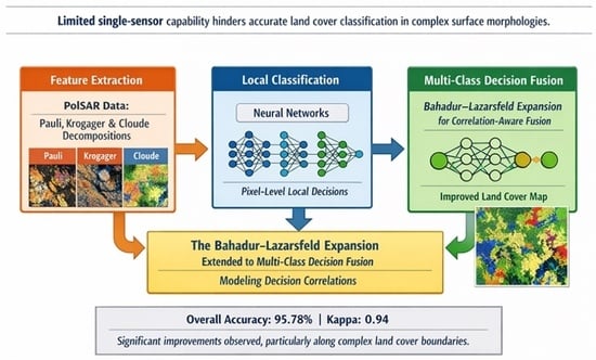
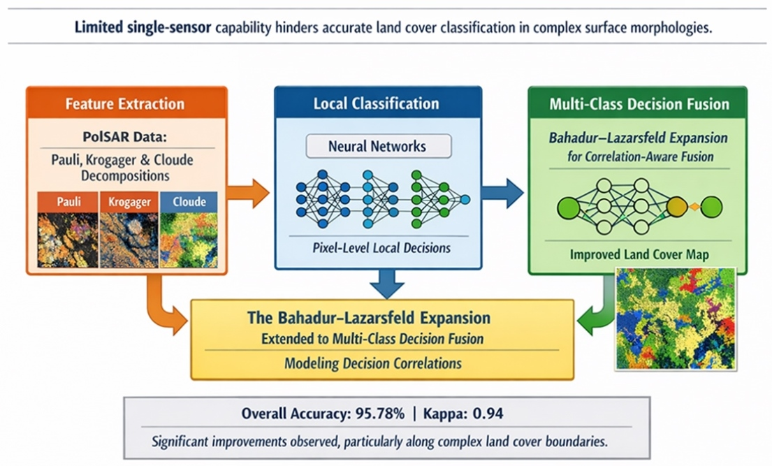
In many land cover classification tasks, the limited precision of individual sensors hinders the accurate separation of certain classes, largely due to the complexity of the Earth’s surface morphology. To mitigate these issues, decision fusion methodologies are employed, allowing data from multiple sensors to be synthesized into robust and more conclusive classification outcomes. This study employs fully polarimetric Synthetic Aperture Radar (PolSAR) imagery and leverages the strengths of three decomposition methods, namely Pauli’s, Krogager’s, and Cloude’s, by extracting their respective components for improved detection. From each decomposition method, three scattering components are derived, enabling the extraction of informative features that describe the scattering behavior associated with various land cover types. The extracted scattering features, treated as independent sensors, were used to train three neural network classifiers. The resulting outputs were then considered as local decisions for each land cover type and subsequently fused through a decision fusion rule to generate more complete and accurate classification results. Experimental results demonstrate that the proposed Multi-Class Bahadur–Lazarsfeld Expansion (MC-BLE) fusion significantly enhances classification performance, achieving an overall accuracy (OA) of 95.78% and a Kappa coefficient of 0.94. Compared to individual classification methods, the fusion notably improved per-class accuracy, particularly for complex land cover boundaries. The core innovation of this work is the transformation of the Bahadur–Lazarsfeld Expansion (BLE), originally designed for binary decision fusion into a multi-class framework capable of addressing multiple land cover types, resulting in a more effective and reliable decision fusion strategy.

1. Introduction

Earth monitoring has been a central focus of scientific research for decades, driven by the need to understand and respond to continuous climate and geomorphological changes. These changes highlight the importance of developing advanced remote sensing methods capable of detecting, classifying, and interpreting evolving environmental scenarios. The use of diverse datasets such as fully polarimetric Synthetic Aperture Radar (PolSAR), optical imagery, and other sensor modalities offers significant opportunities to enhance our understanding of the Earth’s surface through applications including land cover classification, ecological mapping, and sea–land observation. Despite these advances, the complexity of the Earth’s morphology and the limitations of individual sensors often hinder accurate class separation. To address these challenges, researchers have increasingly explored multi-sensor integration and decision fusion approaches, which combine complementary information to achieve more robust and reliable land cover classification results. This study builds upon these efforts by focusing on decision-level fusion to improve classification accuracy and resilience.

Recent advances in remote sensing have increasingly focused on integrating diverse datasets and developing new methodologies to enhance classification performance. For instance, Tsutsumida et al. [1] combined Sentinel-1 and Sentinel-2 imagery with the Dynamic World dataset and demonstrated that the Gradient-Boosted Decision Tree (GBDT) classification, when fused with CNN-based probabilities, not only improved accuracy but also reduced the salt-and-pepper effect that often arises in pixel-based methods. At the same time, the problem of limited and representative training data has been tackled through automated sample generation. Cui et al. [2] introduced the Automatic Generation of Training Samples and Machine Learning (AGTML) approach, which integrates automatic training sample generation with machine learning on Google Earth Engine. Their method achieved overall accuracy (OA) above 90% and showed robustness across regions and sensors, outperforming global land cover products and enabling more scalable classification.

Beyond improvements in training data, decision-level fusion has become an important strategy to improve classification outcomes. Samadzadegan et al. [3] proposed a decision-based fusion method for pan-sharpened, very-high-resolution imagery, using self-guidance filtering and edge information to combine multiple base images. Their results confirmed that decision fusion can successfully balance spectral and spatial qualities, producing outputs superior to those of individual pan-sharpening methods. Further, multimodal data integration has advanced significantly through collaborative fusion frameworks. Zhang et al. [4] developed the Feature–Decision Collaborative Fusion Network (FDCFNet), which combines hyperspectral and LiDAR data by integrating shared and complementary features at the feature level, while dynamically weighting decisions at the decision level. This approach demonstrated improved classification accuracy on benchmark datasets, highlighting the effectiveness of combining feature- and decision-level strategies. Deep learning has further pushed the boundaries of classification accuracy. Vohra and Tiwari [5] developed a multi-fusion Dense Transpose Convolutional Network (MF-DTCFCN) with feature alignment, achieving nearly 99% accuracy on Sentinel-2 data. Their framework demonstrates how feature-level fusion combined with deep networks can overcome the challenges of large-scale feature spaces in high-resolution imagery. Along similar lines, Chen et al. [6] emphasized the value of multi-temporal information, showing that Gradient Tree Boost classifiers applied to multi-season Sentinel data can capture heterogeneous land use patterns with accuracies above 95%. Other studies have explored advanced architecture tailored for complex data. Yin et al. [7] proposed a multi-scale pixel- and super pixel-level method combining adaptive attention with graph convolution, enabling more flexible modeling of spectral–spatial dependencies in hyperspectral images. In parallel, Farahnakian et al. [8] demonstrated that CNN-based fusion of multisource and multiresolution data, including optical, radar, and airborne LiDAR, can address highly imbalanced datasets in ecological applications such as peatland classification. The latest developments in agricultural and environmental monitoring have also emphasized the role of deep learning combined with novel fusion strategies. For instance, Albarakati et al. [9] introduced a network-level self-attention fusion model for agricultural land cover classification, achieving highly accurate results across multiple benchmark datasets by combining optimized self-attention CNN architectures with advanced feature selection strategies. Similarly, Su et al. [10] developed an iterative semi-supervised learning framework for coastal wetland mapping, which integrated super-pixel segmentation with multi-classifier ensembles to improve classification accuracy even with very limited labeled data. This type of semi-supervised strategy is particularly important in real-world settings where large, annotated datasets are not always available.

Urban environments represent another challenging case due to their heterogeneous land use patterns. Fayaz et al. [11] leveraged transfer learning on high-resolution imagery using fine-tuned CNNs, demonstrating significant improvements in urban land classification tasks. Quan et al. [12] addressed the difficulties of multimodal fusion by proposing a cross-modal strategy that combines SAR and optical data at the feature level through PCA-based transformations and attention mechanisms, effectively enhancing classification results. Bhatt and Bhatt [13] also emphasized the importance of lightweight deep learning architectures such as ResNet50 combined with PCA-based dimensionality reductions, which improved computational efficiency while maintaining competitive accuracy. The fusion of optical and radar data has been particularly successful in urban and land cover applications. Ahmad et al. [14] applied a simple layer-stacking fusion with an XGBoost classifier to extract urban impervious surfaces, obtaining higher accuracy compared to single-sensor approaches and outperforming global reference products. Extending this line of research, Irfan et al. [15] systematically compared early and late fusion strategies for SAR-optical integration, showing that early fusion provides superior performance by enabling synergistic low-level feature extraction and reducing modality-specific limitations such as optical cloud obstruction and SAR speckle noise.

Collectively, these studies highlight the transition of land cover classification research toward multi-sensor, multi-scale, and fusion-driven approaches, where each modality provides complementary information to overcome the shortcomings of single-sensor methods. Despite the success of these advanced frameworks, one major limitation remains: most of the methods rely heavily on feature-level or decision-level fusion tailored to specific tasks, but they do not explicitly model the statistical correlations among classifier outputs. To address this gap, we extend the classical Bahadur–Lazarsfeld Expansion (BLE) framework, originally formulated for binary decision fusion, to the multi-class domain by encoding each multi-class decision output into a multivariate binary vector, thereby preserving the binary structure inherent to the original BLE formulation. This novel adaptation enables effective fusion of correlated sensor decisions at the pixel level, providing a more reliable and interpretable solution for land cover classification.

It is also worth mentioning that various decomposition methods [16,17,18,19] have been developed to describe the biophysical scattering behavior of SAR data, forming the foundation of modern target characterization and image classification. In this context, Cloude and Pottier’s entropy/anisotropy/alpha (H/A/α) decomposition [20], Krogager’s orthogonal elliptic basis decomposition [21], and the Pauli basis representation [22] are the three core methods used in this work and presented analytically in the main framework of the paper. Beyond these, numerous other model-based and coherent decomposition techniques further enrich the field. Freeman and Durden’s three-component scattering power model [23] provides a physically intuitive description of surface, double-bounce, and volume scattering under reflection symmetry, while Yamaguchi’s four-component extension [24] incorporates helix scattering and improved volume modeling for complex environments. Cameron et al. [25] introduced a coherent decomposition of the scattering matrix into nonreciprocal, maximum symmetric, and minimum symmetric components, showing that any resolution cell can be represented by at most three equivalent scatterers. Additional contributions include Van Zyl’s covariance-based decomposition for azimuthally symmetric natural terrain [26] and Touzi’s extension of the Kennaugh–Huynen Coherent Target Decomposition (CTD) for both coherent and partially coherent scattering [27].

In the following sections, we present our study. Section 2 outlines the region of interest (ROI) and the materials utilized. Section 3 elaborates on the preprocessing of PolSAR data, and a reference is made to the decomposition methods used as characteristics for the feature extraction. In Section 4, we refer to the classifiers we used and the results of each individual classifier. In Section 5, we briefly present the classic binary Bahadur–Lazarsfeld Expansion (BLE) for decision fusion. In Section 6, we introduce the mathematical background underlying our proposed Multi-Class Bahadur–Lazarsfeld Expansion (MC-BLE) decision fusion method and we present the overall experimental results obtained in the fusion center. Also, the advantages and disadvantages of each methodology are discussed, providing a compact comparative analysis. Section 7 discusses the results of our study, highlighting potential imperfections and explaining the underlying reasons, while Section 8 presents the overall conclusions of this work and outlines possible directions for future research.

2. Study Area and Materials

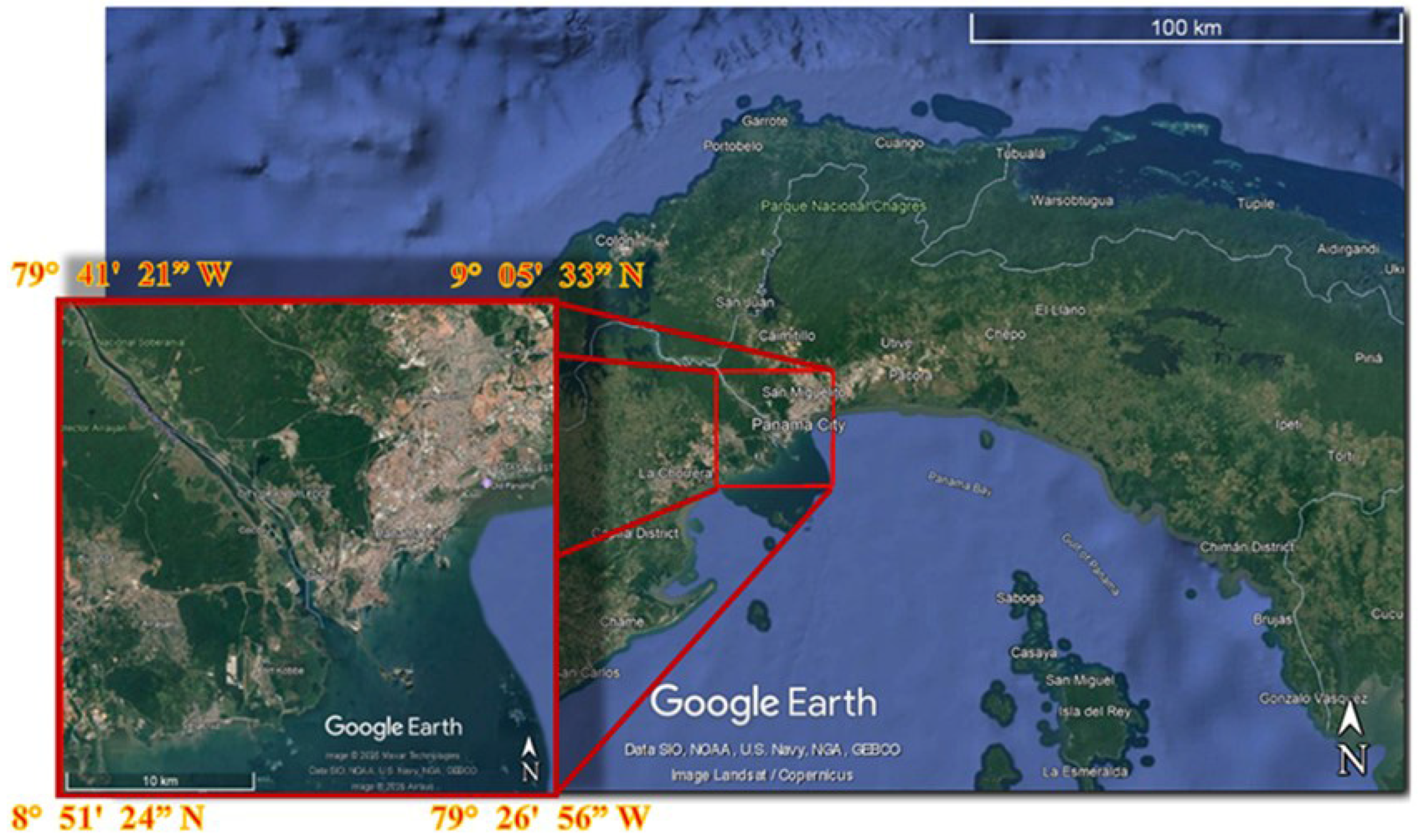
The study was conducted in the broader area of Panama City, defined by the geographic extent from 79°41′21″W to 79°26′56″W longitude and from 9°05′33″N to 8°51′24″N latitude. This region encompasses four dominant land cover classes: urban areas, forest, bare land, and sea. The spatial extent of the study area is illustrated in Figure 1. For the analysis, we utilized satellite data from the Advanced Land Observing Satellite (ALOS). The selected dataset corresponds to an absolute orbit number of 27,527, with incidence angles ranging from 22.76° (near range) to 25.02° (far range). Specifically, an ALOS PALSAR P1.1 Single Look Complex (SLC) product was acquired on 26 March 2011. The data were collected in L-band with a PLR beam mode, offering a spatial resolution of 30 m. All four polarizations (VV, VH, HV, and HH) were employed to support the study objectives. The ALOS PALSAR imagery was freely obtained from the Alaska Satellite Facility (ASF) data portal (https://search.asf.alaska.edu, accessed on 15 September 2025).

3. Preprocessing Feature Extraction

As previously discussed, polarimetric SAR decomposition techniques were employed for feature extraction. Each decomposition method provides three distinct scattering components, which can be utilized as inputs for training classification models. In particular, the combined use of Pauli, Krogager, and Cloude–Pottier decompositions enable highly accurate discrimination between natural and man-made land cover types. The following section presents the decomposition techniques applied in this study, along with a concise overview of the preprocessing steps, to facilitate a clear understanding of the proposed approach.

3.1. Pauli’s Decomposition

The fundamental idea behind the Pauli decomposition is to express the scattering matrix $\left[S\right]$ of each pixel as a combination of elementary scattering matrices, where each component represents a distinct deterministic scattering mechanism [22,28,29]. In the conventional orthogonal linear polarization basis $\left(h,v\right)$, and under the assumption that $S_{hv}=S_{vh}$, the Pauli basis elements $\left[S_a\right],\left[S_b\right],\left[S_c\right]$ can be defined using the following three $2\times 2$ matrices:

$$\left[S_a\right]={\displaystyle \frac{1}{\sqrt{2}}}\left[\begin{array}{cc}1& 0\\ 0& 1\end{array}\right]$$

(1)

$$\left[S_b\right]={\displaystyle \frac{1}{\sqrt{2}}}\left[\begin{array}{cc}1& 0\\ 0& -1\end{array}\right]$$

(2)

$$\left[S_c\right]={\displaystyle \frac{1}{\sqrt{2}}}\left[\begin{array}{cc}0& 1\\ 1& 0\end{array}\right]$$

(3)

Consequently, given a measured scattering matrix $\left[S\right]$, it can be represented as follows:

$$\left[S\right]=\left[\begin{array}{cc}{S}_{hh}& S_{hv}\\ S_{hv}& S_{vv}\end{array}\right]=\alpha \left[S_a\right]+\beta \left[S_b\right]+\gamma \left[S_c\right]$$

(4)

where $S_{hh}$ denotes the horizontal-to-horizontal polarized backscattering component, $S_{hv}$ represents the cross-polarized scattering from horizontal to vertical polarization (equal to $S_{vh}$), and $S_{vv}$ corresponds to the vertical-to-vertical polarized backscattering component. The corresponding scattering coefficients are then computed as follows:

$$\alpha ={\displaystyle \frac{S_{hh}+S_{vv}}{\sqrt{2}}}$$

(5)

$$\beta ={\displaystyle \frac{S_{hh}-S_{vv}}{\sqrt{2}}}$$

(6)

$$\gamma =\sqrt{2}{S}_{hv}$$

(7)

The matrix $\left[S_a\right]$ corresponds to the scattering behavior of a sphere, a flat plate, or a trihedral reflector. In this case, the coefficient $\alpha$ represents the power scattered by targets dominated by single- or odd-bounce scattering mechanisms. The second matrix, $\left[S_b\right]$, describes the scattering from a dihedral reflector oriented at 0°, with the coefficient $\beta$ quantifying the power scattered by such targets. The third matrix, $\left[S_c\right]$, represents the scattering mechanism of a dihedral reflector oriented at 45°, where the coefficient $\gamma$ corresponds to scatterers that return orthogonal polarization–volume scattering being a typical example. This relationship is summarized in

Table 1. Pauli bases and the corresponding meaning [30].

Pauli Basis	Meaning
$S_a$	Single- or odd-bounce scattering: This occurs when a radar signal interacts with a target and undergoes a single reflection or bounce before reaching the radar sensor.
$S_b$	Double- or even-bounce scattering: This can happen, for instance, when radar waves hit a surface, reflect off, and then reflect again off another surface before returning to the sensor.
$S_c$	Volume scattering: This type of scattering is more complex and involves multiple interactions within the target volume, leading to a scattering signal that does not follow a simple direct path (forest canopy).

.

Pauli Color-Coded Representation

The polarimetric information contained in the scattering matrix can be visualized by combining the intensities $\mid S_{hh}{\mid }^2$, $\mid S_{vv}{\mid }^2$, and $2\mid S_{hv}{\mid }^2$ into a single RGB image. However, a major limitation of this approach is the difficulty of directly interpreting the physical meaning of the resulting image in terms of these raw intensity values. To overcome this, an alternative approach is to construct the RGB image using the intensities $\mid \alpha {\mid }^2$, $\mid \beta {\mid }^2$, and $\mid \gamma {\mid }^2$, which correspond to specific physical scattering mechanisms as described in Table 1. The most commonly used coding scheme for this representation is:

$${\left|\beta \right|}^2\to red {\left|\gamma \right|}^2\to green {\left|\alpha \right|}^2\to blue$$

(8)

3.2. Krogager’s Decomposition

Interpreting SAR images, particularly fully polarimetric SAR data, is a complex task [31]. The purpose of polarimetric decomposition is to express the scattering matrix (in the case of coherent decomposition) or, when a second-order analysis is required, the covariance matrix (in incoherent decomposition) as a combination of canonical scattering mechanisms. This approach provides a clearer and more physically meaningful interpretation of the scattering behavior.

Let $S\left(x,y\right)$ represent a $2\times 2$ scattering matrix. A coherent polarimetric decomposition can then be formulated as:

$$S\left(x,y\right)=\sum _{m=1}^M{c}_m{S}_m\left(x,y\right)$$

(9)

In this framework, $S_m\left(x,y\right)$ represents the scattering response of the $m$-th canonical target, while $c_m$ denotes its corresponding weight in the linear combination that reconstructs $S\left(x,y\right)$. Here, $M$ is the total number of components, and $x$ and $y$ are the spatial coordinates. The Krogager polarimetric decomposition is defined using the circular polarization scattering matrix $S_{\left(R,L\right)}\left(x,y\right)$, where $R$ and $L$ correspond to the right-handed and left-handed circular polarization components, respectively. In monostatic radar systems, such as SAR, the scattering matrix is symmetric. As a result, the $S_{\left(R,L\right)}\left(x,y\right)$ components can be expressed in terms of linear polarization components as follows [32]:

$$S_{RR}\left(x, y\right)={\displaystyle \frac{S_{HH}\left(x, y\right)-S_{VV}\left(x, y\right)}{2}}+i{S}_{HV}\left(x, y\right),$$

(10)

$$S_{LL}\left(x, y\right)={\displaystyle \frac{S_{HH}\left(x, y\right)-S_{VV}\left(x, y\right)}{2}}-i{S}_{HV}\left(x, y\right),$$

(11)

$$S_{RL}\left(x, y\right)=S_{LR}\left(x, y\right)={\displaystyle \frac{S_{HH}\left(x, y\right)+S_{VV}\left(x, y\right)}{2}},$$

(12)

where $i$ denotes the imaginary unit, and following [33] with the $\left(x,y\right)$ dependence omitted for clarity the Krogager polarimetric decomposition is expressed as:

$$S_{\left(R,L\right)}=\left[\begin{array}{cc}{S}_{RR}& S_{RL}\\ S_{LR}& S_{LL}\end{array}\right]=e^{i\varphi }\left\{k_s{e}^{i{\varphi }_s}\left[\begin{array}{cc}0& i\\ i& 0\end{array}\right]+k_d\left[\begin{array}{cc}{e}^{i{2}_{\eta }}& 0\\ 0& {-e}^{-i{2}_{\eta }}\end{array}\right]+k_h\left[\begin{array}{cc}{e}^{i{2}_{\eta }}& 0\\ 0& 0\end{array}\right]\right\}$$

(13)

Here, $k_s$, $k_d$, and $k_h$ are real-valued coefficients representing the scattering contributions from a sphere, a diplane, and a helix, respectively. The term $\varphi$ is the absolute phase, which depends on the distance between the target and the sensor. ${\varphi }_s$ denotes the phase shift in the sphere relative to the diplane and helix components, while $\eta$ represents their orientation angle. These scattering coefficients $k_s$, $k_d$, and $k_h$ can be computed from the circular polarization scattering components as described in [34].

$$k_s=\left|S_{RL}\right|,$$

(14)

$$k_d=\min \left(\left|S_{RR}\right|,\left|S_{LL}\right|\right),$$

(15)

$$k_h=\mathrm{a}\mathrm{b}\mathrm{s}\left(\left|S_{RR}\right|,\left|S_{LL}\right|\right)$$

(16)

where the symbol $\left|·\right|$ denotes the modulus of a complex quantity and $abs\left(\cdot \right)$ represents the absolute value.

3.3. Cloude’s Decomposition

Cloude and Pottier introduced a method for extracting the mean scattering mechanism using the eigenvalue–eigenvector decomposition of the coherence matrix [20,35]. Building on this concept, they defined a set of polarimetric parameters, namely the entropy (H), anisotropy (A), and the scattering angles α and β. These parameters are essential for characterizing and distinguishing different scattering mechanisms in fully polarimetric SAR (Synthetic Aperture Radar) data, thereby facilitating target identification and classification. The foundation of this analysis lies in the $2\times 2$ complex scattering matrix $S$, as expressed in Equation (17).

$$\left[S\right]=\left[\begin{array}{cc}{S}_{hh}& S_{hv}\\ S_{hv}& S_{vv}\end{array}\right]$$

(17)

In the vectorial representation, the complex scattering matrix can be expressed in the Pauli basis as the following vector (18):

$${\overrightarrow{k}}_{3P}={\displaystyle \frac{1}{\sqrt{2}}}{\left[S_{hh}+S_{vv} S_{hh}- S_{vv} 2S_{hv}\right]}^T$$

(18)

where the $T$ refers to the transpose operation. To derive the entropy ($H$) and alpha ($\alpha$) parameters, the coherency matrix must be constructed based on ${\overrightarrow{k}}_{3P}$. The coherency matrix formulated in the Pauli basis is expressed in Equation (19).

$$\left[T\right]=〈{\overrightarrow{k}}_{3P}{\overrightarrow{k}}_{3P}^T〉={\displaystyle \frac{1}{2}}\left[\begin{array}{ccc}〈{\left|S_{hh}+S_{vv}\right|}^2〉& 〈\left(S_{hh}+S_{vv}\right){\left(S_{hh}-S_{vv}\right)}^{*}〉& 2〈\left(S_{hh}+S_{vv}\right){S_{hv}}^{*}〉\\ 〈\left(S_{hh}-S_{vv}\right){\left(S_{hh}+S_{vv}\right)}^{*}〉& 〈{\left|S_{hh}-S_{vv}\right|}^2〉& 2〈\left(S_{hh}-S_{vv}\right){S_{hv}}^{*}〉\\ 2〈S_{hv}{\left(S_{hh}+S_{vv}\right)}^{*}〉& 2〈S_{hv}{\left(S_{hh}-S_{vv}\right)}^{*}〉& 4〈{\left|S_{hv}\right|}^2〉\end{array}\right]$$

(19)

The matrix $T$ is Hermitian and positive semidefinite. Its eigenvalues and corresponding eigenvectors form the basis for computing the polarimetric classification parameters. According to the Cloude–Pottier decomposition, the coherency matrix can be expressed as a combination of three independent scattering mechanisms: surface scattering, double-bounce scattering, and volume scattering. The relative contribution of each mechanism is determined through the analysis of the matrix eigenvalues.

Building on the eigenvalue–eigenvector analysis of the coherency matrix introduced by Cloude and Pottier [20,35,36], the individual scattering mechanisms can be further visualized and quantified in terms of their scattering power contributions. Since the eigen-decomposition of the coherency matrix $\left[T\right]$ provides three orthogonal scattering mechanisms, each eigenvalue ${\lambda }_i$ corresponds to the power carried by one independent scattering process.

The relative contributions of these mechanisms can be represented as normalized scattering powers by Equation (20):

$$P_i={\displaystyle \frac{{\lambda }_i}{\sum _{j=1}^3{\lambda }_j}},i=\mathrm{1,2},3$$

(20)

where $P_i$ denotes the fractional power of each scattering mechanism.

The alpha ($\alpha$) angle ranges from 0° to 90° and is used to characterize the dominant scattering mechanism. When $\alpha =0°$, the scattering corresponds to a planar (surface) reflector. At $\alpha =45°$, the scattering behavior resembles that of a dipole. Values of $\alpha$ between 0° and 45° indicate scattering from irregular or moderately rough surfaces, while values between 45° and 90° are associated with double-bounce scattering mechanisms [36]. The eigenvalues of the coherency matrix, denoted as ${\overrightarrow{e}}_i$, are expressed in Equation (21) [35,36].

$${\overrightarrow{e}}_i=\exp \left(i{\varphi }_i\right)\left[\begin{array}{c}\cos a_i\\ \sin a_i\cos {\beta }_i\exp \left(i{\delta }_i\right)\\ \sin a_i\sin {\beta }_i \exp \left(i{\gamma }_i\right)\end{array}\right]$$

(21)

Here, $\delta$ represents the phase difference between $S_{hh}+S_{vv}$ and $S_{hh}-S_{vv}$, while $\gamma$ denotes the phase difference between $S_{hh}+S_{vv}$ and $S_{hv}$. The term $\varphi$ corresponds to the decomposition phase associated with $S_{hh}+S_{vv}$. The mean alpha angle is defined as follows:

$$\overrightarrow{a}=P_1{a}_1+P_2{a}_2+P_3{a}_3$$

(22)

The $a_i$ is the alpha angle corresponding to the eigenvector ${\overrightarrow{e}}_i$.

According to the Cloude decomposition, these three dominant mechanisms are typically interpreted as:

• Surface scattering (associated with low α angles, representing single-bounce reflections on smooth surfaces);
• Double-bounce scattering (associated with high α angles, resulting from interactions between vertical and horizontal structures);
• Volume scattering (associated with intermediate α angles, due to randomly oriented scatterers such as vegetation).

In practice, the Cloude decomposition is constructed by assigning the power of each dominant scattering mechanism to one color channel:

$$\mathrm{RGB}=\left[P_{\mathrm{dbl}},\hspace{0.17em}{P}_{\mathrm{vol}},\hspace{0.17em}{P}_{\mathrm{surf}}\right]$$

where

• $P_{\mathrm{dbl}}$ (red channel) corresponds to double-bounce scattering power;

• $P_{\mathrm{vol}}$ (green channel) corresponds to volume scattering power;

• $P_{\mathrm{surf}}$ (blue channel) corresponds to surface scattering power.

This composite enables a physical interpretation of the scene:

• Red tones indicate built-up or urban regions dominated by double-bounce scattering.
• Green tones correspond to vegetation and forested areas dominated by volume scattering.
• Blue tones highlight water bodies or bare soil where surface scattering dominates.

Based on the theory of previous studies, we can assume that the Krogager decomposition is particularly effective among various coherent polarimetric decompositions in discriminating man-made targets from natural targets [34,37]. However, it lacks the ability to distinguish between different types of man-made targets. On the other hand, Pauli’s decomposition can distinguish natural targets very well [38]. In addition, the Cloude–Pottier [22] decomposition provides complementary information by quantifying the degree of scattering randomness (entropy, H) and the dominant scattering mechanism (mean alpha angle, α) through eigenvalue decomposition of the coherency matrix. This statistical decomposition is particularly powerful for characterizing complex scattering environments such as mixed natural covers and vegetation, where multiple scattering mechanisms coexist. However, it is less effective in differentiating specific man-made scatterer types and can be sensitive to spatial averaging and noise. Therefore, the combination of Krogager, Pauli, and Cloude decompositions offers a more complete scattering description, covering complementary strengths for our study area, which contains a variety of mixed land cover types.

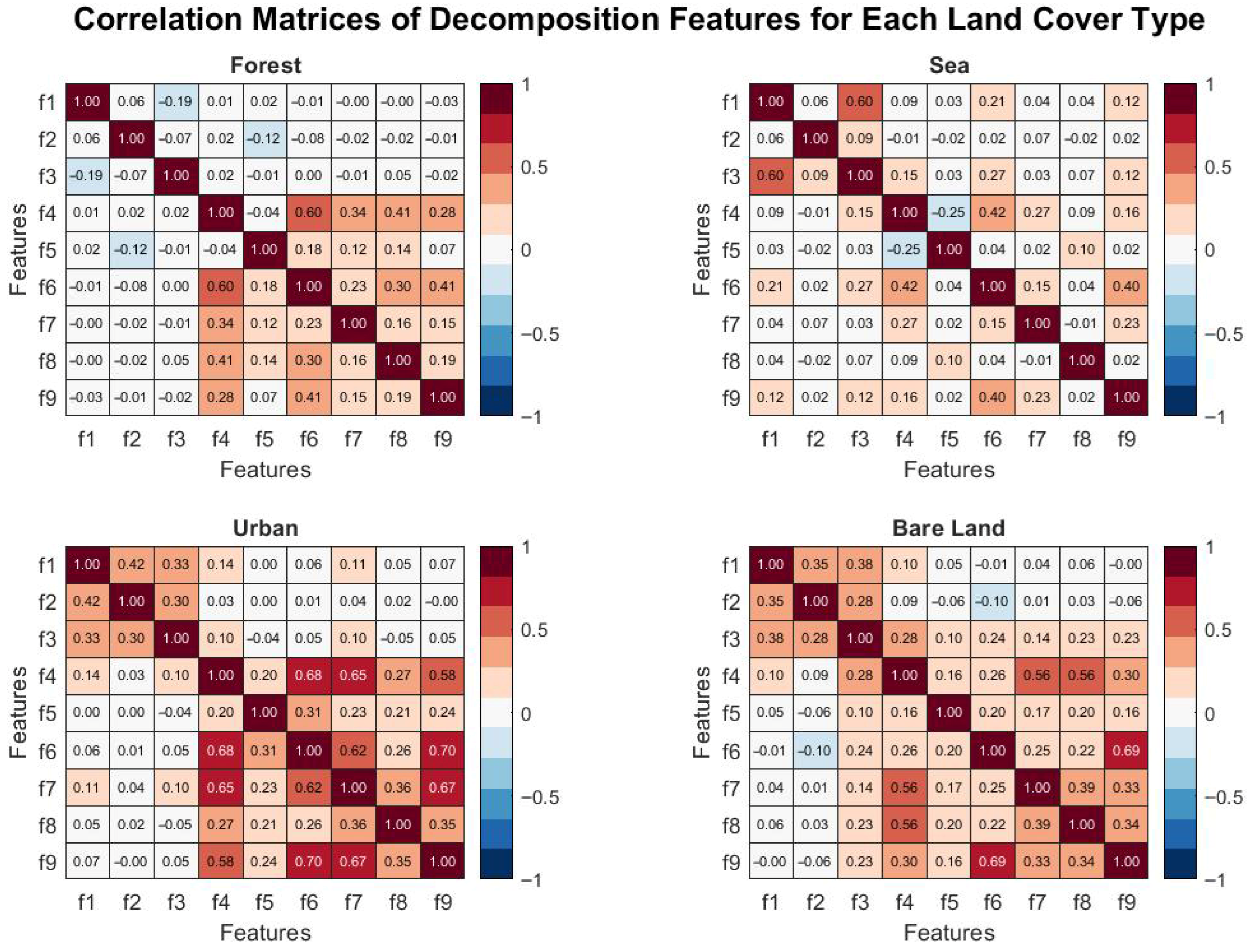
Although this information satisfactorily frames the scattering behavior of each decomposition method, we decided to delve into the root of our training samples to check the within and across correlation of decomposition features as shown to Figure 2 below:

The analysis presented in Figure 2 was carried out between the nine features extracted from the three decomposition methods (Cloude, Krogager, and Pauli) in order to investigate possible relationships among them for each land cover type. The analysis was performed separately for the four land cover classes: forest, sea, urban, and bare land. The resulting correlation matrices in Figure 2 reveal distinct patterns of relationships depending on the physical scattering mechanisms dominating each surface.

For the forest class, the correlation coefficients were generally low both within and across decomposition methods, suggesting that the features carry mostly independent information. This behavior is expected since vegetation produces complex volume scattering, leading to diverse responses across the different decompositions. However, a notable exception is observed between features f4 and f6, which show a strong positive correlation (r ≈ 0.6). This suggests that these two features capture similar scattering characteristics, possibly related to volume scattering effects typical of dense vegetation. In the sea class, where surface scattering dominates, stronger correlations were observed within the Cloude decomposition (up to r ≈ 0.6) and moderate correlations among the others, reflecting the overall homogeneity of the sea surface. The urban class showed moderate-to-high correlations, particularly between features from the Krogager and Pauli decompositions (r ≈ 0.65–0.70), which can be attributed to the double-bounce effects caused by vertical man-made structures. Finally, bare land exhibited intermediate correlation values, with some evident relationships between Krogager and Pauli (r ≈ 0.60–0.70), indicating that certain features respond similarly to the scattering characteristics of soil and rough terrain.

Overall, it can be observed that as the scene becomes more homogeneous (e.g., sea), the correlation among features tends to increase, while in more heterogeneous surfaces (e.g., forest), the features appear more independent and therefore more complementary. This observation is particularly relevant for the subsequent decision fusion stage, as it highlights that correlation between features, and consequently between classifier outputs, should be considered, especially when the sources of information are not completely independent.

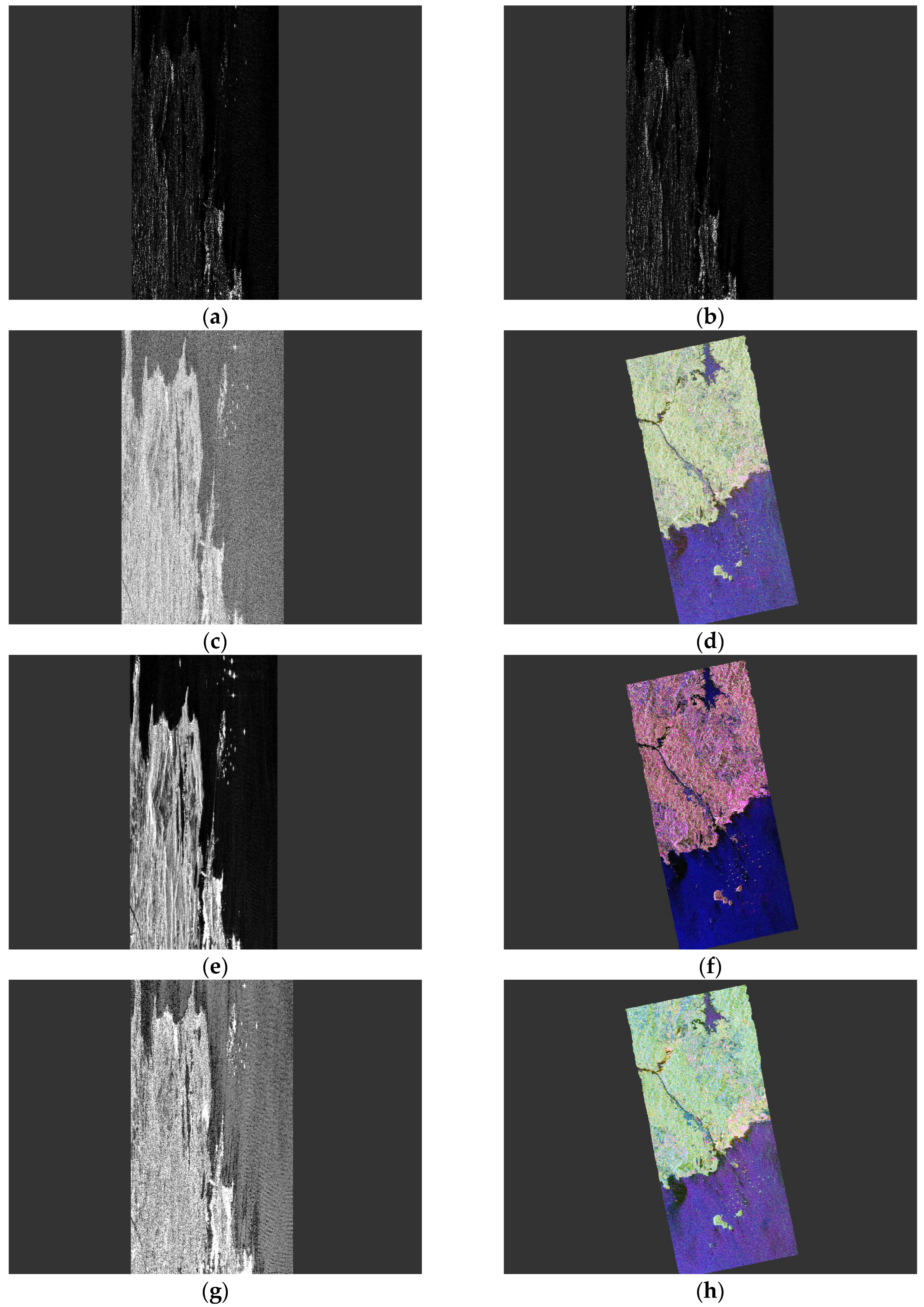
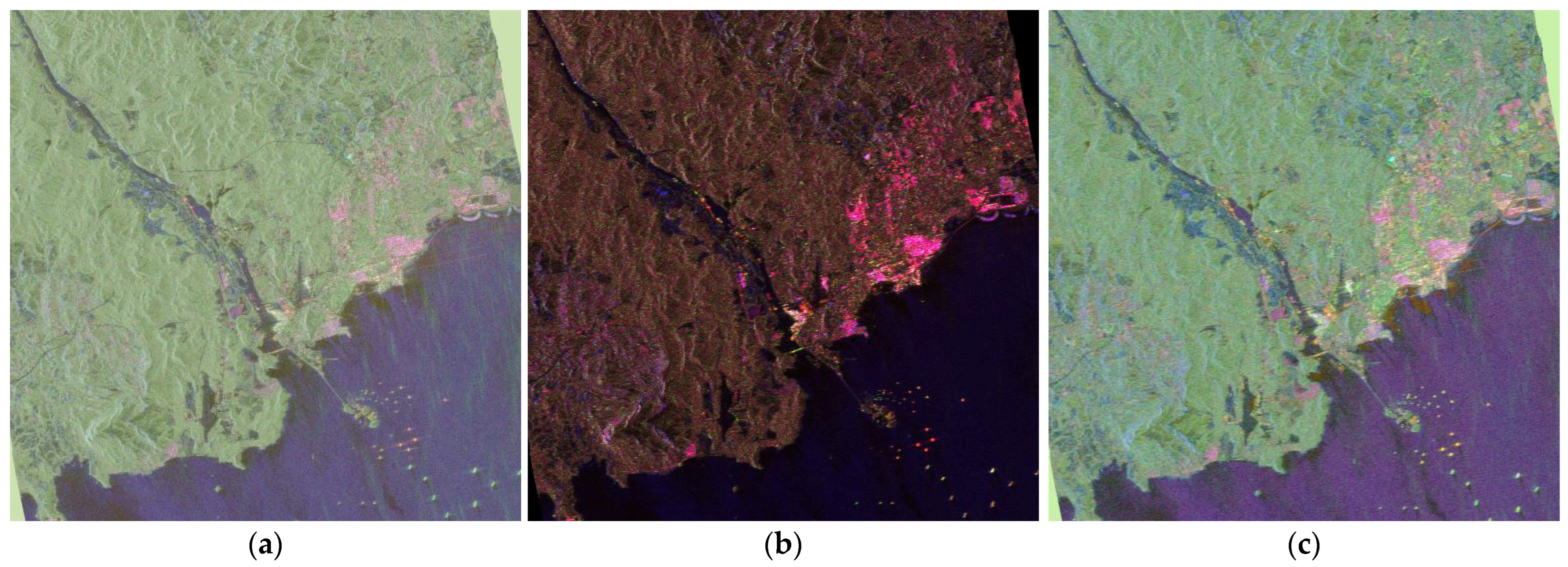
After understanding the inter-feature correlations, we are in a position to present the more practical side of our journey: the extensive preprocessing that Single-Look Complex (SLC) PolSAR data, shown in Figure 3a, undergoes to extract this meaningful information. Using version 12.0.1 of the Sentinel Application Platform (SNAP), we apply a structured workflow that includes radiometric calibration [39], Pauli, Krogager, and Cloude decompositions, followed by geometric Doppler terrain correction [40]. Radiometric calibration is essential for converting raw digital values into physically meaningful units. This process adjusts the SAR image so that pixel values accurately represent the radar backscatter of the reflecting surface, while still preserving geometric distortions, as shown in Figure 3b. Next, the three decomposition methods are applied to transform the complex polarimetric matrices into three distinct components for each method (see one of the components in Figure 3c,e,g). This transformation provides a visual, intuitive representation of polarimetric information, making it easier to interpret scattering mechanisms within the radar data. Finally, Geometric Doppler terrain correction is employed to address geometric distortions caused by a varying topography. Using a Digital Elevation Model (DEM) [41], this correction adjusts for uneven terrain, ensuring that radar reflections align with accurate geographic coordinates. The result is georeferenced RGB datasets (Figure 3d,f,h), which are crucial for precise spatial analysis and scientific interpretation.

4. Multi-Class Classification

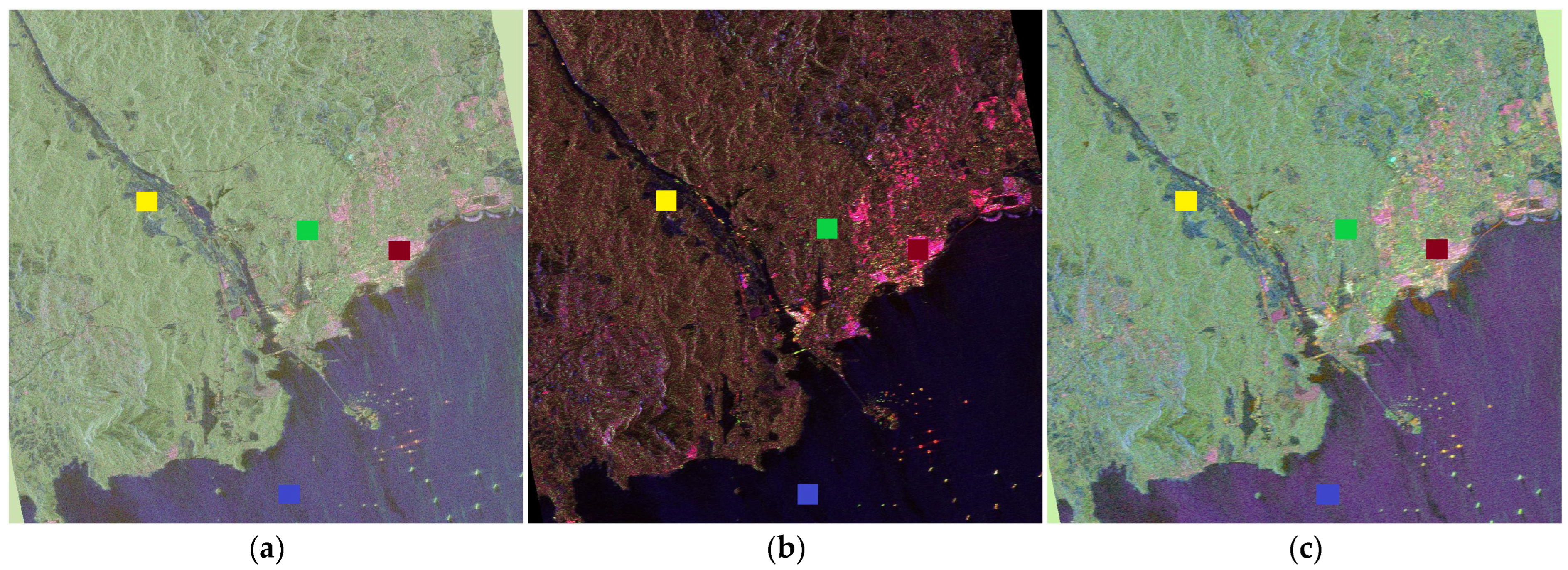
For the classification process, we employed as input features the scattering components obtained from Pauli (Figure 4a), Krogager (Figure 4b), and Cloude (Figure 4c) decompositions, extracted using the SNAP software (version 12.0.0). These components represented as $\alpha ,\beta ,\gamma$ (Pauli), $k_s,{ k}_d, k_h$ (Krogager), and $P_{dbl},{ P}_{vol},{ P}_{surf}$ (Cloude) correspond to the intensities of the respective scattering coefficients and are expressed in decibels (dB).To handle the negative dB values and prepare the data for color visualization, a normalization procedure was applied to each component. Specifically, their histograms were adjusted to rescale the intensity values to a range between 0 and 255, ensuring compatibility with standard color mapping schemes.

After normalization, the scattering components were used as feature inputs for each pixel across the entire study area, giving each pixel a distinct signature composed of three features per decomposition method. To improve computational efficiency, four representative 40 × 40-pixel windows were selected, each corresponding to one of the main land cover types in the study region. Specifically, urban areas were labeled red, the sea in blue, bare land in yellow, and forests in green, as illustrated in Figure 5 below.

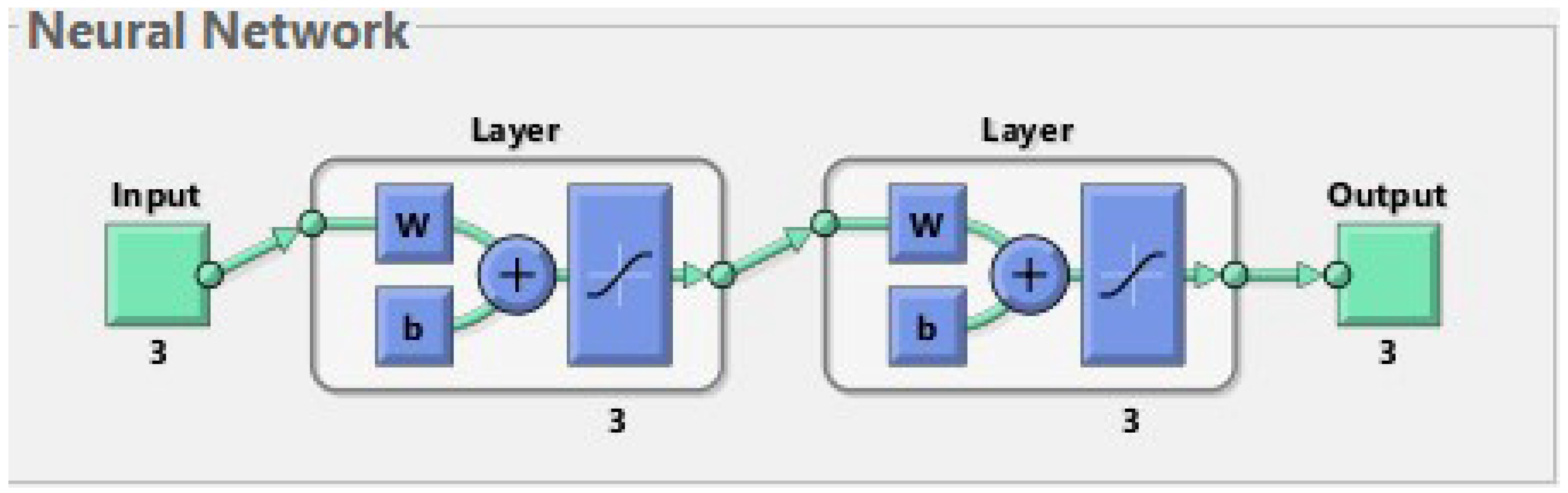
For each polarimetric decomposition (Pauli, Cloude, and Krogager), a two-layer feedforward neural network (NN) [42] (Figure 6) was implemented to classify the pixels into four land cover types. This NN includes three input neurons, one hidden layer with three neurons, and an output layer with three neurons. Both layers employed the hyperbolic tangent sigmoid (tansig) activation function. The network was trained using the Levenberg–Marquardt algorithm (trainlm) [43] with mean squared error (MSE) [44] as the performance function, a maximum of 500 epochs, a learning rate of 0.01, and a minimum gradient threshold of $1\times {10}^{-20}$. During training, 80% of the data was used for learning and 20% for testing (

Table 2. Number of pixels used for each class for training and testing.

Class	Number Assigned	Training Pixels	Testing Pixels
Bare Land	1	1280	320
Urban	2	1280	320
Sea	3	1280	320
Forest	4	1280	320

). The three output neurons produced binary-coded vectors (e.g., 001, 010, 011, 100) representing the four land cover classes, bare land, urban, sea, and forest, which were subsequently converted to their decimal equivalents (1, 2, 3, 4) to generate the final class labels. This binary output representation not only ensured compact multi-class encoding but also enabled each output neuron to be interpreted as an independent binary decision source, forming the basis for the subsequent decision fusion analysis.

Table 3. Confusion matrix exploited by NN classification for Pauli’s decomposition method.

	Class	1	2	3	4	Total
True Class	1	187	21	34	78	320
	2	11	241	1	67	320
	3	10	0	310	0	320
	4	23	31	0	266	320
	Total	231	293	345	411	1280
	Predicted Class

,

Table 4. Confusion matrix exploited by NN classification for Cloude’s decomposition method.

	Class	1	2	3	4	Total
True Class	1	237	2	43	38	320
	2	4	232	0	84	320
	3	7	0	313	0	320
	4	21	1	0	298	320
	Total	269	235	356	420	1280
	Predicted Class

,

Table 5. Confusion matrix exploited by NN classification for Krogager’s decomposition method.

	Class	1	2	3	4	Total
True Class	1	277	0	1	42	320
	2	0	274	0	46	320
	3	1	0	319	0	320
	4	0	2	0	318	320
	Total	288	276	320	406	1280
	Predicted Class

and

Table 6. Quantitative information of each decomposition methodology.

Methodology	OA (%)	Kappa	Bare land (C1) (%)	Urban (C2) (%)	Sea (C3) (%)	Forest (C4) (%)
Pauli	78.44	0.713	58.44	75.31	96.88	83.13
Cloude	84.38	0.792	74.06	72.50	97.81	93.13
Krogager	92.81	0.905	86.56	85.63	99.69	99.38

present the confusion matrices and quantitative information such as OA, class-wise accuracy and Kappa coefficient, a metric that signifies the agreement between the classifier’s predictions and the true labels. All this information was generated by the neural network classifier for each of the polarimetric decomposition methods. These matrices serve as the foundation for our analysis, allowing us to quantify the rate of correct classification and identify specific patterns of misclassification that arise from similarities in terrain scattering properties or mixed-pixel phenomena.

The classification performance, as summarized by the matrices above, clearly demonstrates the varying discriminative power of the features derived from the three polarimetric decomposition methods: Pauli, Cloude, and Krogager. The Krogager decomposition yielded the highest OA, establishing itself as the strongest individual classifier, followed by Cloude, with Pauli performing the poorest. This hierarchy underscores the critical dependence of the neural network’s performance on the quality of the initial feature extraction. Notably, all three methods achieved near-perfect classification for sea (Class 3), confirming the inherent separability of water due to its distinct and uniform scattering signature.

The primary challenge lies in separating the three terrestrial classes: bare land (1), urban (2), and forest (4). The weaker Pauli features exhibited the most significant confusion, classifying only 187 out of 320 bare land samples correctly, with major errors resulting from misclassifications into forest (78 samples) and urban (34 samples), which can be justified due to the existence of greenery in the urban fabric. Conversely, the Krogager features dramatically resolved this ambiguity, boosting the correct classification rate for bare land to 277, and for forest to 318. This improvement confirms that the Krogager method successfully generates features that better capture the subtle scattering properties necessary to differentiate between complex scattering environments like forests and urban centers, and the more delicate signatures of bare surfaces.

Crucially, the decision to pursue decision fusion is empirically supported by the analysis of the misclassification patterns. While the Krogager method is the superior performer, it is not flawless; its remaining errors are specific and localized, such as misclassifying 42 bare land samples as forest. The weaker classifiers, however, exhibit diverse and distinct error distributions. For instance, the errors from the Cloude and Pauli methods often arise from different scattering mechanisms than the Krogager-based errors.

Following the results obtained from the tables above, it clearly establishes a hierarchy of performance among the methods. The Krogager classifier achieved the highest OA at 92.81% and the strongest statistical agreement, indicated by a Kappa coefficient of 0.905. This Kappa value signifies near-perfect agreement between the classifier’s predictions and the true labels, providing high confidence in the Krogager-based features. In contrast, the Pauli decomposition yielded the lowest at 78.44% and a significantly lower Kappa value of 0.713, confirming its status as the weakest individual classifier. The Cloude method sits precisely between these two, with a robustness of 84.38% and a Kappa of 0.792, validating its role as an intermediate performer.

This complementarity of errors is the foundational premise for decision fusion. By intelligently combining the decisions of the less accurate Pauli and Cloude classifiers with the superior Krogager classifier, the fused system is hypothesized to leverage the unique discriminative information available in each feature set. The goal is to resolve ambiguities that persist even in the strongest individual classification, ultimately leading to an ensemble accuracy that surpasses the performance of the best individual Krogager-based result.

5. Classic Binary BLE for Decision Fusion

In this section, the classical binary [45,46] Bahadur–Lazarsfeld Expansion approach is applied for decision fusion across multiple sensors. The BLE binary framework operates by independently training a one-vs.-rest classifier for each land cover type, producing marginal probabilities for each class. These probabilities are then combined using BLE to model inter-class correlations and generate global fused decisions.

Including in this work the classical binary BLE [46] serves several purposes: it provides a well-established baseline for comparison, allows an evaluation of the operational and statistical differences between binary and multi-class formulations, and demonstrates the advantages of the proposed multi-class BLE methodology in terms of efficiency, coherence, and practical deployment. While binary BLE is computationally more intensive and requires synthetic “not-landcover” labels for each class, multi-class BLE achieves similar fusion results with a single training per sensor, using only the true land cover labels, making it a more scalable and statistically principled solution.

5.1. Classification from the Sensors

For each decomposition method, binary classifiers were trained to distinguish each land cover type from all other classes. Specifically, Pauli, Cloude, and Krogager decompositions were used as input features. Importantly, the same land cover windows employed in the multi-class experiments were used here (Figure 5), and the neural network architecture was identical to the one used for multi-class classification (Figure 6). This ensures that any differences in performance are attributable exclusively to the binary versus multi-class formulation, rather than differences in input data or model architecture. Classifier performance was evaluated using confusion matrices and both per-class and class-vs.-all (non-class) accuracies.

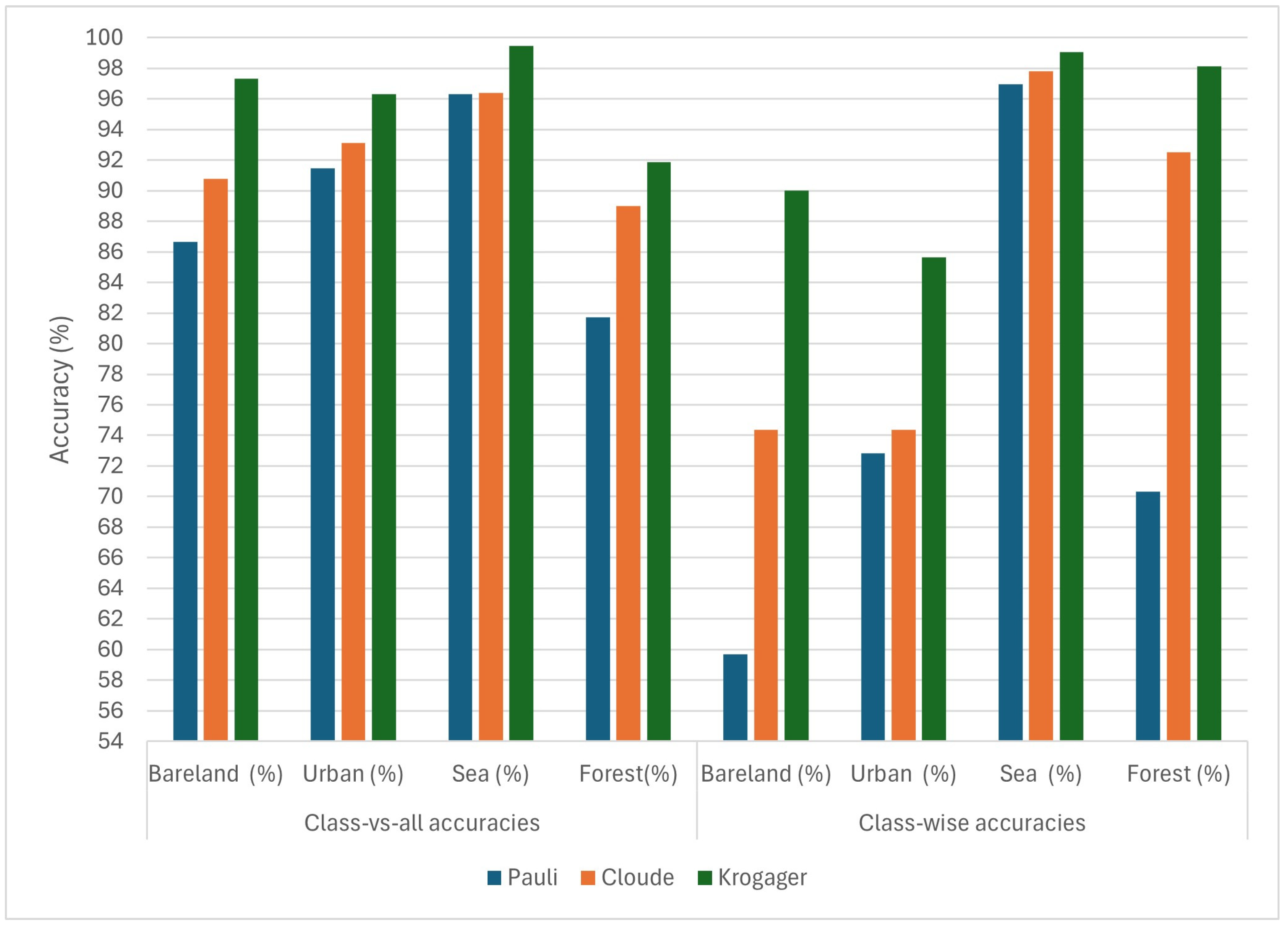
The Pauli sensor results in Figure 7 show that class-vs.-all accuracies range from 81.72% (forest) to 96.33% (sea), with class-wise accuracies reflecting lower performance for bare land (59.69%) and urban (72.81%) due to imbalanced negative classes in the binary formulation. Cloude sensor results improved overall performance, with class-vs.-all accuracies between 88.98% (forest) and 96.41% (sea), and class-wise accuracies reaching 92.5% for forest and 97.81% for sea. Krogager sensor results demonstrated the highest individual sensor performance, with class-vs.-all accuracies from 91.87% (forest) to 99.45% (sea) and class-wise accuracies up to 99.06% for sea and 98.12% for forest. These results confirm that all three sensors provide strong discriminative power individually, and that the setup is directly comparable to the multi-class methodology, setting the stage for subsequent fusion using the classical binary BLE approach.

5.2. Fusion Using Classic Binary BLE

The classical binary BLE framework performs decision fusion by modeling the joint distribution of independent binary classifiers for each land cover type. In this approach, a separate binary classifier is trained for each class, treating it as the positive class while grouping all other land cover types into a single “not-class” category. This procedure results in four one-vs.-rest classifiers per sensor, producing marginal probabilities that are subsequently combined using the BLE.

For each binary classifier corresponding to land cover type $C_k$, the binary decision outputs are collected into decision vectors:

$$x^{\left(k\right)}=\left\{x_1^{\left(k\right)},x_2^{\left(k\right)}, x_3^{\left(k\right)}\right\}=$$

$$=\left\{\begin{array}{c}\begin{array}{ccc}{x}_{1 1}^{\left(k\right)}& x_{2 1}^{\left(k\right)}& x_{3 1}^{\left(k\right)}\\ x_{1 2}^{\left(k\right)}& x_{2 2}^{\left(k\right)}& x_{3 2}^{\left(k\right)}\\ x_{1 3}^{\left(k\right)}& x_{2 3}^{\left(k\right)}& x_{3 3}^{\left(k\right)}\end{array}\\ \begin{array}{ccc}⋮& ⋮& ⋮\\ x_{1 M}^{\left(k\right)}& x_{2 M}^{\left(k\right)}& x_{3 M}^{\left(k\right)}\end{array}\end{array}\right\}$$

(23)

where $x^{\left(k\right)}$ is the decision vector for each sample of a certain class $k$, $N=3$ is the number of classifier sensors (Pauli, Cloude, and Krogager) and M is the number of pixels under investigation.

Each set of samples which belong to class $C_k$ is used to estimate the class-conditional marginal probabilities $p_i^{\left(k\right)}$, which characterize the distribution of each classifier’s binary output. These training samples are employed exclusively for parameter estimation, including the marginal probabilities and the correlation terms required by the Bahadur–Lazarsfeld Expansion (BLE) model. During classification, the independent probability component $P_{indep}\left(x^{\left(k\right)}\right|C_k)$ is evaluated separately for each observed 3-bit decision vector using the estimated parameters. Thus, although multiple samples belong to the same class, the likelihood is defined and computed for a single realization of the classifier decision vector, and each observed decision vector is classified independently.

The class-conditional marginal probability for each binary variable is estimated as the mean value across all samples labeled as $C_k$:

$$p_i^{\left(k\right)}={\displaystyle \frac{1}{\mid D_k\mid }}\sum _{x\in D_k}{x}_i^{\left(k\right)},i=1,\dots ,3$$

(24)

where $D_k$ is the set of samples belonging to the class $C_k$. These marginal probabilities reflect the frequency with which each binary classifier predicts the class (positive or not). To avoid numerical instabilities, probabilities are constrained within:

$${10}^{-8}<p_i^{\left(k\right)}<1-{10}^{-8}.$$

The independent probability component for a sample $x^{\left(k\right)}$ is then:

$$P_{indep}\left(x^{\left(k\right)}∣C_k\right)=\prod _{i=1}^3\left(p_i^{\left(k\right)}{)}^{x_i^{\left(k\right)}}\right(1-p_i^{\left(k\right)}{)}^{1-x_i^{\left(k\right)}}.$$

(25)

Each binary variable is standardized to have zero mean and unit variance:

$$z_i^{\left(k\right)}={\displaystyle \frac{x_i^{\left(k\right)}-p_i^{\left(k\right)}}{\sqrt{p_i^{\left(k\right)}\left(1-p_i^{\left(k\right)}\right)}}}.$$

(26)

Pair-wise correlation coefficients between classifier outputs are then computed as:

$${\gamma }_{ij}^{\left(k\right)}={\displaystyle \frac{1}{\mid D_k\mid }}\sum _{x\in D_k}{z}_i^{\left(k\right)}{z}_j^{\left(k\right)},i<j.$$

(27)

Higher-order correlations (third order and above) are typically omitted in classical binary BLE implementations due to the reduced dimensionality of the binary decision vectors. The class-conditional likelihood for each sample is therefore:

$$\widehat{P}\left(x^{\left(k\right)}∣C_k\right)=P_{indep}\left(x^{\left(k\right)}∣C_k\right)\left[1+\sum _{i<j}{\gamma }_{ij}^{\left(k\right)}{z}_i^{\left(k\right)}{z}_j^{\left(k\right)}\right]$$

(28)

Here, the independent term models the reliability of each binary classifier individually, while the pair-wise term captures dependencies between classifier outputs.

After estimating class-conditional likelihoods for all classes, the normalized posterior probability is computed using Bayes’s theorem:

$$P\left(C_k∣x^{\left(k\right)}\right)={\displaystyle \frac{\widehat{P}\left(x^{\left(k\right)}∣C_k\right)P\left(C_k\right)}{\sum _{j=1}^2\widehat{P}\left(x^{\left(k\right)}∣C_j\right)P\left(C_j\right)}}.$$

(29)

where $P\left(C_k\right)$ represents the prior probability of the positive class, typically assumed equal for all classes in the absence of prior knowledge. The posterior probabilities are normalized so that they sum to one across both classes.

The final decision rule assigns each sample to the class with the maximum posterior probability:

$$\widehat{C}=\arg \underset{2}{\max }P\left(C_k∣x^{\left(k\right)}\right).$$

(30)

This framework is repeated independently for each binary classifier, resulting in four BLEs and corresponding fusion steps per sensor, in contrast to the MC-BLE approach which performs a single multi-class fusion.

5.3. Results of Classic Binary BLE Fusion

After applying the classical binary BLE framework, the per-class confusion matrices and accuracies for each land cover type are obtained and presented in

Table 7. Presentation of the per-class overall accuracies (class vs. not-class) and the per-class accuracies (correctly classified pixels within each class) obtained using the classical binary BLE framework.

Land Cover Type	Bare Land	Urban	Sea	Forest	Overall Class Accuracy
Overall Accuracy (Class vs. Not-Class)	95.94%	98.28%	99.61%	94.06%	-
Per-Class Accuracy (Correct Pixels within Class)	95.62%	95.31%	100%	96.56%	96.87%

below:

The results in Table 7 indicate that the binary BLE fusion achieves very high OA, with the sea and forest classes showing near-perfect classification. the bare land and urban classes, while slightly lower, remain above 95% accuracy, confirming that the fusion framework effectively combines the information from multiple sensors.

6. Multi-Class Bahadur–Lazarsfeld Expansion for Decision Fusion

This chapter describes the proposed framework for fusing decisions from multiple independent classifiers using a multi-class shortened version of the BLE [45]. The methodology extends the traditional BLE [46], which models multivariate binary distributions, to a multi-class scenario through one-hot encoding, thereby capturing higher-order dependencies among the individual classifier outputs. The classification system comprises $M$ individual classifiers and $k$ mutually exclusive classes. The fusion process transforms the $M$ multi-class decisions into a single binary vector upon which the BLE is applied.

6.1. “One-Hot” Encoding of Local Decisions

To enable the application of the BLE, the multi-class decisions produced by the classifiers were transformed into a multivariate binary representation. This allows the modeling of joint distributions and pair-wise correlations among individual classifier outputs.

For each test sample $n$, every classifier $m\in \left\{\mathrm{1,2},\dots ,M\right\}$ produces a discrete class label:

$$d_m^{\left(n\right)}\in \left\{\mathrm{1,2},\dots ,k\right\},$$

where $k$ denotes the number of land cover types and $M$ is the total number of classifiers. In our case, $M=3$ (three classifiers) and $k=4$ (four land cover types, e.g., water, vegetation, urban, and soil).

Each decision $d_m^{\left(n\right)}$ is converted into a $k$-dimensional binary vector ${\mathbf{v}}_m^{\left(n\right)}$:

$${\mathbf{v}}_m^{\left(n\right)}=\left\{v_{m,1}^{\left(n\right)},v_{m,2}^{\left(n\right)},\dots ,v_{m,K}^{\left(n\right)}\right\},$$

(31)

where

$$v_{m,k}^{\left(n\right)}=\left\{\begin{array}{cc}1,& \mathrm{if} d_m^{\left(n\right)}=k,\\ 0,& \mathrm{otherwise}.\end{array}\right.$$

(32)

This encoding ensures that each classifier’s decision is represented in a format compatible with binary correlation modeling. The one-hot vectors of all classifiers are concatenated to form the final decision vector:

$${\mathbf{x}}^{\left(n\right)}=\left\{{\mathbf{v}}_1^{\left(n\right)},{\mathbf{v}}_2^{\left(n\right)},\dots ,{\mathbf{v}}_M^{\left(n\right)}\right\},$$

(33)

resulting in a binary vector of length $M\times k$. For our configuration ($M=3$, $k=4$), each sample’s decision vector becomes:

$${\mathbf{x}}^{\left(n\right)}=\left\{v_{\mathrm{1,1}}^{\left(n\right)},\dots ,v_{\mathrm{1,4}}^{\left(n\right)},v_{\mathrm{2,1}}^{\left(n\right)},\dots ,v_{\mathrm{2,4}}^{\left(n\right)},v_{\mathrm{3,1}}^{\left(n\right)},\dots ,v_{\mathrm{3,4}}^{\left(n\right)}\right\},$$

(34)

which is a 12-dimensional binary vector representing the local decisions of the three classifiers across the four land cover types.

6.2. Estimation of BLE Coefficients

The core of the proposed framework lies in the class-conditional estimation of the parameters required for the MC-BLE. These parameters include the marginal probabilities of each binary variable and the standardized correlation coefficients up to the third order, which capture dependencies among classifier outputs.

To simplify the presentation of the methodology, we assume that each element $v_{m,k}$ of the one-hot encoded decision vectors is hereafter represented as $x_i^{\left(k\right)}$, where $i=\left\{\mathrm{1,2},\dots ,N\right\}$. So, for the estimation of these parameters, for each true class $C_k$, the samples belonging to that class were selected, along with their corresponding decision vectors.

$${\mathbf{x}}^{\left(k\right)}=\left\{x_1^{\left(k\right)},x_2^{\left(k\right)},\dots ,x_N^{\left(k\right)}\right\}.$$

(35)

Here, $N=M\times K$ denotes the total number of binary variables resulting from the one-hot encoding of all classifiers. In our configuration, we have $M=3$ classifiers and $K=4$ land cover types, leading to decision vectors of length $N=12$.

For each binary variable $x_i^{\left(k\right)}$, the class-conditional marginal probability is computed as the mean value across all samples belonging to class $C_k$:

$$p_i^{\left(k\right)}={\displaystyle \frac{1}{\mid D_k\mid }}{\sum }_{\mathbf{x}\in D_k}{x}_i^{\left(k\right)},$$

(36)

with $i\in \left\{1,\dots ,12\right\}$ and $k=\left\{1,\dots ,4\right\}$. Here, $D_k$ represents the set of samples of class $C_k$, and $\mid D_k\mid$ denotes the number of samples in that class. This probability reflects how frequently each binary component (corresponding to a specific classifier–class pair) takes value 1 when the true label is $C_k$. To prevent numerical instability, marginal probabilities were constrained within:

$${10}^{-8}<p_i^{\left(k\right)}<1-{10}^{-8}.$$

Using the estimated marginals, the independent probability product for a given sample ${\mathbf{x}}^{\left(k\right)}$ and class $C_k$ is computed as:

$$P_{indep}\left({\mathbf{x}}^{\left(k\right)}∣C_k\right)=\prod _{i=1}^{12}\left(p_i^{\left(k\right)}{)}^{x_i^{\left(k\right)}}\right(1-p_i^{\left(k\right)}{)}^{1-x_i^{\left(k\right)}}$$

(37)

Each binary variable is then transformed into a standardized variable to ensure zero mean and unit variance within class $C_k$:

$$z_i^{\left(k\right)}={\displaystyle \frac{x_i^{\left(k\right)}-p_i^{\left(k\right)}}{\sqrt{p_i^{\left(k\right)}\left(1-p_i^{\left(k\right)}\right)}}}$$

(38)

These standardized variables are used for estimating the correlation coefficients that describe dependencies between classifier outputs. The pair-wise (second-order) correlation coefficients are computed as the expected value of the product of two standardized variables:

$${\gamma }_{ij}^{\left(k\right)}={\displaystyle \frac{1}{\mid D_k\mid }}{\sum }_{\mathbf{x}\in D_k}{z}_i^{\left(k\right)}{z}_j^{\left(k\right)},for i<j$$

(39)

with $i\in \left\{1,\dots 11\right\},j\in \left\{2,\dots ,12\right\}$. Similarly, the third-order coefficients capture three-way interactions following all the possible triplets $\left(\begin{array}{c}N\\ m\end{array}\right)={\displaystyle \frac{N!}{m!\left(N-m\right)!}}$, which returns a matrix containing all possible combinations of the elements of the 12-bit vector taken m at a time. In our case we have $\left(\begin{array}{c}12\\ 3\end{array}\right)={\displaystyle \frac{12!}{3!9!}}=220$:

$${\gamma }_{ijl}^{\left(k\right)}={\displaystyle \frac{1}{\mid D_k\mid }}\sum _{\mathbf{x}\in D_k}{z}_i^{\left(k\right)}{z}_j^{\left(k\right)}{z}_l^{\left(k\right)}, for i<j<l.$$

(40)

with $i\in \left\{\mathrm{1,2},\dots 10\right\},j\in \left\{\mathrm{2,3},\dots ,11\right\}$ and $l\in \left\{\mathrm{3,4},\dots ,12\right\}$

The pair-wise terms model dependencies between pairs of classifier outputs, while the third-order terms describe more complex interdependencies among three outputs.

By combining the independent component with the estimated correlation terms, the class-conditional likelihood for class $C_k$ is expressed as:

$$\widehat{P}\left({\mathbf{x}}^{\left(k\right)}∣C_k\right)=\underset{independent component}{\underbrace{\prod _{i=1}^{12}\left(p_i^{\left(k\right)}{)}^{x_i^{\left(k\right)}}\right(1-p_i^{\left(k\right)}{)}^{1-x_i^{\left(k\right)}}}}\left[1+\sum _{i<j}{\gamma }_{ij}^{\left(k\right)}{z}_i^{\left(k\right)}{z}_j^{\left(k\right)}+\sum _{i<j<l}{\gamma }_{ijl}^{\left(k\right)}{z}_i^{\left(k\right)}{z}_j^{\left(k\right)}{z}_l^{\left(k\right)}\right].$$

(41)

In this expression:

• ${\gamma }_{ij}^{\left(k\right)}$ represents the pair-wise correlation coefficient between variables $i$ and $j$ for class $C_k$;

• ${\gamma }_{ijl}^{\left(k\right)}$ represents the third-order interaction coefficient;
• The first product term models the independent contribution, while the additive terms model interdependence among classifiers.

This formulation extends the BLE framework to the multi-class case by integrating the correlations derived from one-hot encoded decision vectors, thus enabling the fusion process to account for both individual classifier reliability and inter-classifier dependencies.

6.3. Posterior Probability Estimation and Decision Rule

The fusion process consists of three main steps:

• Computing the class-conditional likelihoods $\widehat{P}\left({\mathbf{x}}^{\left(k\right)}∣C_k\right)$ using the MC-BLE model;
• Converting these likelihoods into posterior probabilities;
• Applying a maximum a posteriori (MAP) decision rule to determine the final fused class label.

After calculating $\widehat{P}\left({\mathbf{x}}^{\left(k\right)}∣C_k\right)$ for all classes $C_k$, the normalized posterior probability is obtained using Bayes’s theorem:

$$P\left(C_k∣{\mathbf{x}}^{\left(k\right)}\right)={\displaystyle \frac{\widehat{P}\left({\mathit{x}}^{\left(k\right)}∣C_k\right)P\left(C_k\right)}{\sum _{j=1}^4\widehat{P}\left({\mathit{x}}^{\left(k\right)}∣C_j\right)P\left(C_j\right)}}$$

(42)

where $P\left(C_k\right)$ represents the prior probability of class $C_k$. In the present study, all classes were assumed to be equally probable, i.e., $P\left(C_k\right)={\displaystyle \frac{1}{K}}$, since no prior class distribution information was available. Normalization ensures that posterior probabilities across all classes sum to one.

Finally, the MAP decision rule assigns each sample to the class with the maximum posterior probability:

$$\widehat{C}=\arg \underset{k}{\max }P\left(C_k∣{\mathbf{x}}^{\left(k\right)}\right)$$

(43)

This decision rule provides an optimal classification under the assumption of equal misclassification costs, yielding the final fused class label for each input sample.

To summarize, the proposed MC-BLE fusion model combines the decisions of the three classifiers by modeling their joint probability distribution through the BLE. Sensor-concatenated outputs are first converted into a 12-dimensional “one-hot” vector, and for each land cover class the marginal probabilities, Equation (36), pair-wise correlations Equation (39), and third-order interactions Equation (40) of the bit-nodes are estimated. During fusion, the BLE model evaluates, for every test sample, the likelihood, Equation (41) that its observed 12-bit pattern was generated under each class. These class-conditional likelihoods are normalized to posteriors Equation (42), and the final fused label is obtained via an argmax selection Equation (43). Fusion improves class-wise accuracy because the BLE learns which combinations of sensor decisions are statistically consistent with each class. Even when one sensor is wrong, the BLE model assigns higher posterior probability to the class whose marginal and correlated structure best explains the observed pattern. This allows the fused decision to surpass the accuracy of each individual classifier, particularly in classes where sensors exhibit complementary or redundant behaviors.

6.4. Experimental Results

In the previous section, we presented the general mathematical formulation of the proposed MC-BL) framework. In this section, we describe the experimental fusion results and compare them with the local classification outcomes of each independent neural network (NN) classifier.

To briefly recap, the experimental setup involved three neural network classifiers, each trained on feature sets derived from distinct polarimetric decomposition methods, namely Pauli’s, Cloude’s, and Krogager’s decompositions. The study area comprises four dominant land cover classes: bare land, urban, sea, and forest. for each class, 320 representative samples were selected, yielding a total of 1280 samples.

Each classifier produced one decision per sample, resulting in an output matrix of dimensions $1280\times 3$, where each column corresponds to a classifier and each entry represents the predicted class label. These categorical outputs were subsequently transformed into a one-hot encoded binary representation of size $1280\times 12$ (three classifiers × four classes). This binary decision matrix served as the input to the MC-BLE fusion model, which computed the joint class-conditional likelihoods and final posterior probabilities for each land cover type. The results are presented at

Table 8. Confusion matrix exploited by MC-BLE.

	Class	1	2	3	4	Total
True Class	1	287	0	1	32	320
	2	0	304	0	16	320
	3	1	0	319	0	320
	4	1	3	0	316	320
	Total	289	307	320	364	1280
	Predicted Class

and

Table 9. Classification performance of the proposed MC-BLE method across four land cover types, showing OA, Kappa coefficient, and per-class accuracy percentages.

Methodology	OA (%)	Kappa	Bare Land (C1) (%)	Urban (C2) (%)	Sea (C3) (%)	Forest (C4) (%)
MC-BLE	95.78	0.9437	89.69	95.00	99.69	98.38

below:

Although our initial results were promising, with OA exceeding 75% across all decomposition methods (78.44% for Pauli’s, 84.38% for Cloude’s, and 92.81% for Krogager’s decomposition) as shown in Table 6, we were confident that the implementation of the proposed MC-BLE fusion methodology could further enhance classification performance.

As confirmed by the results presented in Table 9 and

Table 10. Detailed classification metrics for each land cover class using the MC-BLE method, including recall, precision, F1-score, and false positive rate (FPR).

Class	Recall	Precision	F1-Score	FPR
1 (Bare Land)	0.8969	0.9931	0.9423	0.0021
2 (Urban)	0.9500	0.9902	0.9697	0.0031
3 (Sea)	0.9969	0.9969	0.9969	0.0010
4 (Forest)	0.9875	0.8682	0.9236	0.0500

, our expectations were not only met but exceeded. The MC-BLE approach achieved an OA of 95.78% and a Kappa coefficient of 0.9437, representing an improvement of nearly 3% compared to the most accurate individual classifier (Krogager’s decomposition). This significant gain underscores the effectiveness of the MC-BLE in leveraging complementary information across multiple decomposition methods.

Beyond OA, the most notable improvements were observed in class-wise performance. Specifically, the land cover types that were previously the most frequently misclassified, bare land and urban, exhibited substantial gains. Bare land reached an accuracy of 89.69%, while urban achieved 95.00%, marking remarkable improvements compared to Pauli’s decomposition (55.44% and 75.31%, respectively) and Cloude’s decomposition (74.06% and 72.50%, respectively). The sea and forest classes also demonstrated near-perfect classification, with accuracies of 99.69% and 98.38%, respectively, reflecting the robustness of the MC-BLE methodology across all land cover types.

Detailed evaluation metrics further highlight the effectiveness of the proposed approach. Bare land achieved a recall of 0.8969, precision of 0.9931, F1-score of 0.9423, and a very low false positive rate (FPR) of 0.0021. Urban showed similarly high performance, with a recall of 0.9500, precision of 0.9902, F1-score of 0.9697, and FPR of 0.0031. Sea and forest were classified with exceptional accuracy, with sea attaining perfect recall, precision, and F1-score (0.9969 each) and an FPR of 0.0010, while forest achieved a recall of 0.9875, precision of 0.8682, F1-score of 0.9236, and an FPR of 0.0500.

6.5. Methods Comparison

6.5.1. Comparison of Classic BLE with MC-BLE

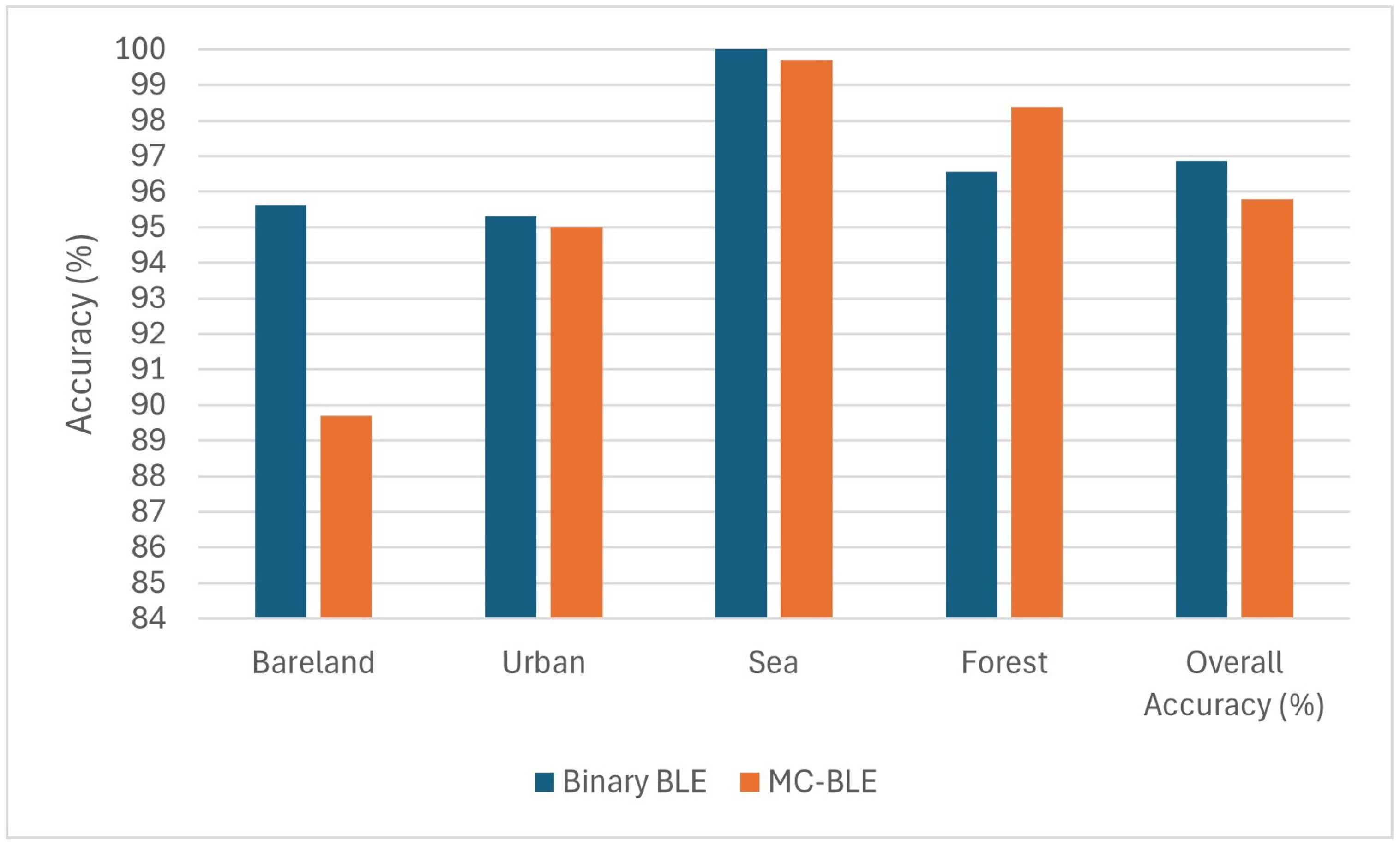
To evaluate the effectiveness of the proposed multi-class BLE (MC-BLE) framework, the classical binary BLE results were compared with the MC-BLE outcomes (Figure 8) obtained under the same experimental conditions. Importantly, both approaches used identical land cover windows and the same neural network architecture for independent sensor classification, ensuring a fair comparison.

From an operational perspective, the MC-BLE requires only a single training procedure per sensor and one fusion execution for all classes, while classical binary BLE necessitates four separate one-vs.-rest trainings per sensor and four BLEs. This reduces both computational load and memory requirements by approximately a factor of four. From a statistical standpoint, the MC-BLE avoids the construction of synthetic “not-class” labels used in binary BLE, relying exclusively on true class labels. This preserves the natural distributions of the land cover types and produces a coherent, normalized probability space across classes. Furthermore, the MC-BLE model has higher-order correlations among all classifiers simultaneously, whereas binary BLE is limited to pair-wise dependencies within each binary problem.

While the OA of binary BLE is slightly higher (96.87% vs. 95.78%), the MC-BLE demonstrates more balanced performance across classes, improving the forest class accuracy (98.38% vs. 96.56%) and maintaining very high accuracy for the sea and urban classes. Combined with the substantial computational efficiency gains and statistical consistency, these results highlight that the MC-BLE is the preferred methodology for multi-sensor land cover decision fusion.

6.5.2. Comparison with Other Multi-Class Methodologies

The proposed MC-BLE method demonstrates superior performance, as shown in

Table 11. Comparison of classification performance between the proposed MC-BLE method and the early and late fusion strategies reported in [15]. Accuracy (Acc), F1-score (F1), and false positive rate (FPR) are provided for each land cover class.

Method	OA (%)	Kappa	Bare Land	Urban	Sea	Forest	Comments
Early Fusion [15]	88.12	–	Acc:66.79–70.18%, F1 <70%	Acc:89+%, F1: 87+%	Acc:94+%, F1:97.10%	Acc:78.36%, F1: 69.83%	Indicative performance; struggles with bare land and forest
Late Fusion [15]	83.96	–	Acc:66.79–70.18%, F1: 59.51%	Acc:89+%, F1: 87+%	Acc:94+%, F1:97.10%	Acc:71.15%, F1: 73.59%	Weaker overall; F1 higher for forest
MC-BLE (Proposed)	95.78	0.9437	Acc: 89.69, F1: 0.94%, FPR: 0.0021	Acc: 95.00, F1:0.97%, FPR: 0.0031	Acc:99.69, F1:0.99%, FPR:0.0010	Acc:98.38, F1:0.92%, FPR:0.0500	Strong improvements across all classes; very low FPR

, compared to the early and late fusion strategies reported in [15], which applied deep learning-based fusion of Sentinel-1 and Sentinel-2 data. Overall, the MC-BLE achieves an accuracy of 95.78% and a Kappa coefficient of 0.9437, substantially outperforming early fusion (OA: 88.12%, F1: 86.53%) and late fusion (OA: 83.96%, F1: 81.87%) from [15]. At the class level, the MC-BLE provides consistently high accuracy across all land cover types, with bare land: 89.69%, urban: 95.00%, sea: 99.69%, and forest: 98.38%, representing notable improvements over the fusion strategies in [15], particularly for challenging classes such as bare land and forest.

Similarly, the per-class F1-scores are considerably higher, reaching 0.9423 for bare land, 0.9697 for urban, 0.9969 for sea, and 0.9236 for forest, while false positive rates (FPR) remain extremely low (<0.05), indicating reliable classification with minimal misclassification. These results highlight that the MC-BLE effectively balances precision and recall, even for classes that were challenging under conventional fusion strategies [15].

This comparison is indicative rather than a direct benchmark, as the study areas, datasets, and experimental setups differ between this work and [15]. Nonetheless, it provides a meaningful perspective on the potential advantages of the proposed MC-BLE method for multi-class land cover classification. Overall, these results clearly demonstrate that the MC-BLE fusion methodology not only improves overall classification accuracy but also significantly enhances the reliability and consistency of land cover classification, particularly for classes that are typically challenging to distinguish.

7. Discussion

The results obtained in this study demonstrate the efficiency and robustness of the proposed MC-BLE framework for multi-sensor land cover decision fusion. By integrating the categorical outputs of three neural network classifiers trained on Pauli, Cloude, and Krogager polarimetric decompositions, the MC-BLE effectively modeled both marginal and higher-order correlations among decision sources. As shown in Table 8, the method achieved an OA of 95.78% and a Kappa coefficient of 0.9437, indicating excellent agreement with ground truth labels. These results confirm the theoretical expectation that correlation-aware fusion can better exploit the complementary nature of polarimetric features, compared to single-sensor or naïve fusion approaches.

A detailed assessment of per-class metrics further highlights the advantages of the MC-BLE. The classes that were traditionally more prone to spectral and textural confusion, bare land (c1) and urban (c2) showed substantial improvements relative to their single-sensor counterparts. While Pauli and Cloude decompositions achieved only 55.44%/74.06% and 75.31%/72.50% accuracy for these two classes (Table 6), the MC-BLE fusion dramatically increased their accuracy to 89.69% and 95.00%, respectively (Table 9). This improvement demonstrates the model’s capacity to reduce sensor-specific ambiguity by capturing correlated decision patterns, consistent with findings in related multi-sensor fusion literature [47,48] where aggregating angular or polarimetric diversity noticeably enhances discrimination in built-up and soil-like regions.

Performance for sea (c3) and forest (C4) classes was near-perfect, with accuracies of 99.69% and 98.38% (Table 9). Their recall, precision, and F1-scores (Table 10) further validate the reliability of the fused classification. In particular, sea achieved 0.9969 across all metrics, while forest showed high recall (0.9875) but comparatively lower precision (0.8682), meaning that although forest pixels were almost always correctly identified (low omission error), some were confused with visually or structurally similar land cover types (higher omission error). This behavior aligns with well-known challenges in polarimetric SAR classification, where forests tend to overlap with other high-entropy scattering mechanisms in rough terrain [49].

The methodological strengths of the MC-BLE come from its principled generalization of the classical BLE. By converting each classifier decision into a one-hot binary vector, the approach enables the direct modeling of dependencies across multiple classes simultaneously. Unlike ensemble learning methods that introduce an additional training stage, the MC-BLE estimates marginal, pair-wise, and third-order correlations directly from classifier outputs. This makes the method not only transparent and interpretable but also computationally efficient. As shown in Section 6.5, the MC-BLE requires only one training per sensor, whereas classical binary BLE requires four one-vs.-rest classifiers per sensor and four separate BLEs. To the best of our knowledge, this is the first work to extend the BLE to the multi-class setting using one-hot encoded outputs, and the advantages of the MC-BLE arise directly from this formulation rather than from prior literature.

The comparison between the two methods (Figure 8) provides further insight. Although binary BLE achieved a marginally higher OA (96.87%), this improvement is partly attributed to the one-vs.-rest formulation where each classifier focuses on a simpler binary task. The MC-BLE, however, provides more balanced performance across all classes, especially improving forest accuracy (98.38% vs. 96.56%) and maintaining high reliability for urban and sea. Furthermore, the MC-BLE avoids the construction of artificial “non-class” categories, producing a more coherent multi-class probability space.

Despite the strong results, several limitations were identified. The experiments were carried out on a single acquisition date. This restricts generalization to multi-temporal scenarios, where seasonal or phenological changes may influence class separability. Estimating third-order correlations requires sufficient samples per class to ensure numerical stability. In cases with limited training data, higher-order estimation may become unreliable, and the one-hot representation increases feature dimensionality proportionally to the number of classes and sensors, which may introduce redundancy for larger-scale problems. Addressing these issues may involve regularized or sparse correlation estimation, dimensionality reduction, or adaptive BLE formulations. Simultaneously, we are currently examining other decomposition models which could be incorporated in the proposed model.

Future extensions will focus on applying the MC-BLE to multi-temporal and multimodal datasets, integrating the MC-BLE within deep learning fusion architectures, exploring scalable BLE variants for large numbers of sensors and classes, and validating performance using additional geographical regions and time periods. These directions can further establish the MC-BLE as a generalizable and efficient framework for correlated decision fusion in Earth observation.

8. Conclusions

This work introduced a novel MC-BLE framework for multi-sensor land cover classification using polarimetric SAR imagery. The method extends the classical BLE formulation from binary to multi-class decision fusion through a one-hot transformation that preserves probabilistic dependencies across all categories. Using three polarimetric decomposition features and neural network classifiers, the MC-BLE effectively captured higher-order correlations, producing a unified probabilistic classification map.

Experimental results demonstrated that the MC-BLE substantially improves classification accuracy compared to individual classifiers and outperforms the classical BLE in terms of computational efficiency, class balance, and statistical consistency. The model achieved a high OA of 95.78%, with near-perfect accuracy for sea and forest classes and significant improvements for bare land and urban classes. These findings confirm that modeling higher-order dependencies yields more robust and reliable fusion performance, especially in challenging land cover scenarios.

Overall, the proposed MC-BLE framework offers a principled, interpretable, and scalable solution to multi-sensor decision fusion in remote sensing. With appropriate extensions toward multi-temporal and large-scale datasets, the MC-BLE has strong potential for integration into operational classification systems and advanced Earth observation pipelines.

References

1. Tsutsumida, N.; Nasahara, K.; Tadono, T.; Birch, T.; Erickson, T. 10-Meter Resolution Land Cover Classification Mapping Using Sentinel-1 & 2 and Dynamic World. In Proceedings of the IGARSS 2023—2023 IEEE International Geoscience and Remote Sensing Symposium, Pasadena, CA, USA, 16–21 July 2023. [Google Scholar] [CrossRef]
2. Cui, Y.; Yang, G.; Zhou, Y.; Zhao, C.; Pan, Y.; Sun, Q.; Gu, X. AGTML: A Novel Approach to Land Cover Classification by Integrating Automatic Generation of Training Samples and Machine Learning Algorithms on Google Earth Engine. Ecol. Indic. 2023, 154, 110904. [Google Scholar] [CrossRef]
3. Samadzadegan, F.; Toosi, A.; Javan, F.D.; Stein, A. Decision-Based Fusion of Pansharpened VHR Satellite Images Using Two-Level Rolling Self-Guidance Filtering and Edge Information. ISPRS Ann. Photogramm. Remote Sens. Spat. Inf. Sci. 2023, X-4/W1-2022, 691–698. [Google Scholar] [CrossRef]
4. Zhang, S.; Meng, X.; Liu, Q.; Yang, G.; Sun, W. Feature-Decision Level Collaborative Fusion Network for Hyperspectral and LiDAR Classification. Remote Sens. 2023, 15, 4148. [Google Scholar] [CrossRef]
5. Vohra, R.; Tiwari, K.C. Land Cover Classification Using Multi-Fusion Based Dense Transpose Convolution in Fully Convolutional Network with Feature Alignment for Remote Sensing Images. Earth Sci. Inform. 2022, 16, 983–1003. [Google Scholar] [CrossRef]
6. Chen, R.; Yang, H.; Yang, G.; Liu, Y.; Zhang, C.; Long, H.; Xu, H.; Meng, Y.; Feng, H. Land-Use Mapping with Multi-Temporal Sentinel Images Based on Google Earth Engine in Southern Xinjiang Uygur Autonomous Region, China. Remote Sens. 2023, 15, 3958. [Google Scholar] [CrossRef]
7. Yin, J.; Liu, X.; Hou, R.; Chen, Q.; Huang, W.; Li, A.; Wang, P. Multiscale Pixel-Level and Superpixel-Level Method for Hyperspectral Image Classification: Adaptive Attention and Parallel Multi-Hop Graph Convolution. Remote Sens. 2023, 15, 4235. [Google Scholar] [CrossRef]
8. Farahnakian, F.; Zelioli, L.; Pitkänen, T.; Pohjankukka, J.; Middleton, M.; Tuominen, S.; Nevalainen, P.; Heikkonen, J. Multistream Convolutional Neural Network Fusion for Pixel-Wise Classification of Peatland. In Proceedings of the 2022 25th International Conference on Information Fusion (FUSION), Charleston, SC, USA, 27–30 June 2023; pp. 1–8. [Google Scholar] [CrossRef]
9. Albarakati, H.M.; Khan, M.A.; Hamza, A.; Khan, F.; Kraiem, N.; Jamel, L.; Almuqren, L.; Alroobaea, R. A Novel Deep Learning Architecture for Agriculture Land Cover and Land Use Classification from Remote Sensing Images Based on Network-Level Fusion of Self-Attention Architecture. IEEE J. Sel. Top. Appl. Earth Obs. Remote Sens. 2024, 17, 6338–6353. [Google Scholar] [CrossRef]
10. Su, H.; Lu, H.; Zheng, P.; Zheng, H.; Xue, Z.; Du, Q. Iterative Semi-Supervised Learning with Few-Shot Samples for Coastal Wetland Land Cover Classification. IEEE Trans. Geosci. Remote Sens. 2024, 62, 1–16. [Google Scholar] [CrossRef]
11. Fayaz, M.; Nam, J.; Dang, L.M.; Song, H.-K.; Moon, H. Land-Cover Classification Using Deep Learning with High-Resolution Remote-Sensing Imagery. Appl. Sci. 2024, 14, 1844. [Google Scholar] [CrossRef]
12. Quan, Y.; Zhang, R.; Li, J.; Ji, S.; Guo, H.; Yu, A. Learning SAR-Optical Cross Modal Features for Land Cover Classification. Remote Sens. 2024, 16, 431. [Google Scholar] [CrossRef]
13. Bhatt, A.; Bhatt, V.T. Dcrff-Lhrf: An Improvised Methodology for Efficient Land-Cover Classification on Eurosat Dataset. Multim. Tools Appl. 2023, 83, 54001–54025. [Google Scholar] [CrossRef]
14. Ahmad, M.N.; Shao, Z.; Javed, A.; Ahmad, I.; Islam, F.; Skilodimou, H.D.; Bathrellos, G.D. Optical–SAR Data Fusion Based on Simple Layer Stacking and the XGBoost Algorithm to Extract Urban Impervious Surfaces in Global Alpha Cities. Remote Sens. 2024, 16, 873. [Google Scholar] [CrossRef]
15. Irfan, A.; Li, Y.; E, X.; Sun, G. Land Use and Land Cover Classification with Deep Learning-Based Fusion of SAR and Optical Data. Remote Sens. 2025, 17, 1298. [Google Scholar] [CrossRef]
16. Karachristos, K.; Koukiou, G.; Anastassopoulos, V. A Review on PolSAR Decompositions for Feature Extraction. J. Imaging 2024, 10, 75. [Google Scholar] [CrossRef]
17. Kouroupis, G.; Anastassopoulos, V. Polarimetric Decomposition for the Selection of Persistent Scatterers. Remote Sens. Lett. 2016, 8, 271–279. [Google Scholar] [CrossRef]
18. Kouroupis, G.; Anastassopoulos, V. Scatterer Characterization Based on the Condiagonalization of the Sinclair Backscattering Matrix. Prog. Electromagn. Res. M 2019, 85, 59–69. [Google Scholar] [CrossRef]
19. Karachristos, K.; Koukiou, G.; Anastassopoulos, V. Fully Polarimetric Land Cover Classification Based on Hidden Markov Models Trained with Multiple Observations. Adv. Remote. Sens. 2021, 10, 102–114. [Google Scholar] [CrossRef]
20. Ouarzeddine, M.; Belhdj Aissa, A.; Souissi, B.; Belkhider, M.; Boulahbal, S. Polarimetric Classification Using the Cloude/Pottier Decomposition. In Proceedings of the 2nd International Workshop POLINSAR 2005 (ESA SP-586), Frascati, Italy, 17–21 January 2005; Volume 586, p. 16. [Google Scholar]
21. Krogager, E. New Decomposition of the Radar Target Scattering Matrix. Electron. Lett. 1990, 26, 1525. [Google Scholar] [CrossRef]
22. Cloude, S.R.; Pottier, E. A Review of Target Decomposition Theorems in Radar Polarimetry. IEEE Trans. Geosci. Remote Sens. 1996, 34, 498–518. [Google Scholar] [CrossRef]
23. Freeman, A.; Durden, S.L. A Three-Component Scattering Model for Polarimetric SAR Data. IEEE Trans. Geosci. Remote Sens. 1998, 36, 963–973. [Google Scholar] [CrossRef]
24. Yamaguchi, Y.; Moriyama, T.; Ishido, M.; Yamada, H. Four-Component Scattering Model for Polarimetric SAR Image Decomposition. IEEE Trans. Geosci. Remote Sens. 2005, 43, 1699–1706. [Google Scholar] [CrossRef]
25. Cameron, W.L.; Rais, H. Conservative Polarimetric Scatterers and Their Role in Incorrect Extensions of the Cameron Decomposition. IEEE Trans. Geosci. Remote Sens. 2006, 44, 3506–3516. [Google Scholar] [CrossRef]
26. Vanzyl, J.J. Application of Cloude’s Target Decomposition Theorem to Polarimetric Imaging Radar Data. In Proceedings of the Radar Polarimetry, San Diego, CA, USA, 12 February 1993; p. 1748. [Google Scholar] [CrossRef]
27. Touzi, R. Target Scattering Decomposition in Terms of Roll-Invariant Target Parameters. IEEE Trans. Geosci. Remote Sens. 2007, 45, 73–84. [Google Scholar] [CrossRef]
28. Chen, S.-W.; Li, Y.; Wang, X.; Xiao, S.; Sato, M. Modeling and Interpretation of Scattering Mechanisms in Polarimetric Synthetic Aperture Radar: Advances and Perspectives. IEEE Signal Process. Mag. 2014, 31, 79–89. [Google Scholar] [CrossRef]
29. Sun, X.; Song, H.; Wang, R.; Li, N. High-Resolution Polarimetric SAR Image Decomposition of Urban Areas Based on a POA Correction Method. Remote Sens. Lett. 2018, 9, 363–372. [Google Scholar] [CrossRef]
30. Zhang, Y.; Wu, L.; Wei, G. A New Classifier for Polarimetric SAR Images. Prog. Electromagn. Res. 2009, 94, 83–104. [Google Scholar] [CrossRef]
31. Gaglione, D.; Clemente, C.; Pallotta, L.; Proudler, I.; De Maio, A.; Soraghan, J.J. Krogager Decomposition and Pseudo-Zernike Moments for Polarimetric Distributed ATR. In Proceedings of the 2014 Sensor Signal Processing for Defence (SSPD), Edinburgh, UK, 8–9 September 2014. [Google Scholar] [CrossRef]
32. Milan, J.M. Book Review [Review of “Principles of Modern Radar—Basic Principles (Richards, M.A., Eds, et al.; 2010)]. IEEE Aerosp. Electron. Syst. Mag. 2013, 28, 40–42. [Google Scholar] [CrossRef]
33. Hellmann, M.; Krogager, E. Comparison of Decompositions for Pol-SAR Image Interpretation. In Proceedings of the IGARSS 2000, IEEE 2000 International Geoscience and Remote Sensing Symposium. Taking the Pulse of the Planet: The Role of Remote Sensing in Managing the Environment. Proceedings (Cat. No.00CH37120), Honolulu, HI, USA, 24–28 July 2000; p. 3. [Google Scholar] [CrossRef]
34. Alberga, V.; Krogager, E.; Chandra, M.; Wanielik, G. Potential of Coherent Decompositions in SAR Polarimetry and Interferometry. In Proceedings of the IGARSS 2004, 2004 IEEE International Geoscience and Remote Sensing Symposium, Anchorage, AK, USA, 20–24 September 2004; p. 3. [Google Scholar] [CrossRef]
35. Cloude, S.R.; Pottier, E. An Entropy Based Classification Scheme for Land Applications of Polarimetric SAR. IEEE Trans. Geosci. Remote Sens. 1997, 35, 68–78. [Google Scholar] [CrossRef]
36. Hajnsek, I.; Pottier, E.; Cloude, S.R. Inversion of Surface Parameters from Polarimetric SAR. IEEE Trans. Geosci. Remote Sens. 2003, 41, 727–744. [Google Scholar] [CrossRef]
37. Wei, Q.; Jian-Jun, C.; Hong-Zhong, Z.; Feng, Z. Target Decomposition for Fully Polarimetric Wideband Radar System. In Proceedings of the IEEE 10th International Conference on Signal Processing Proceedings, Beijing, China, 24–28 October 2010. [Google Scholar] [CrossRef]
38. Zhang, L.; Zhang, J.; Zou, B.; Zhang, Y. Comparison of Methods for Target Detection and Applications Using Polarimetric SAR Image. Piers Online 2008, 4, 140–145. [Google Scholar]
39. Kumar, D. Urban Objects Detection from C-Band Synthetic Aperture Radar (SAR) Satellite Images through Simulating Filter Properties. Sci. Rep. 2021, 11, 1–24. [Google Scholar] [CrossRef] [PubMed]
40. Jiang, W.; Yu, A.; Dong, Z.; Wang, Q. Comparison and Analysis of Geometric Correction Models of Spaceborne SAR. Sensors 2016, 16, 973. [Google Scholar] [CrossRef]
41. Makineci, H.B.; Karabörk, H. Evaluation Digital Elevation Model Generated by Synthetic Aperture Radar Data. Int. Arch. Photogramm. Remote Sens. Spat. Inf. Sci. 2016, XLI-B1, 57–62. [Google Scholar] [CrossRef][Green Version]
42. Singh, J.; Banerjee, R. A Study on Single and Multi-Layer Perceptron Neural Network. In Proceedings of the 2019 3rd International Conference on Computing Methodologies and Communication (ICCMC), Erode, India, 27–29 March 2019. [Google Scholar] [CrossRef]
43. Bilski, J.; Smoląg, J.; Kowalczyk, B.; Grzanek, K.; Izonin, I. Fast Computational Approach to the Levenberg-Marquardt Algorithm for Training Feedforward Neural Networks. J. Artif. Intell. Soft Comput. Res. 2023, 13, 45–61. [Google Scholar] [CrossRef]
44. Sai, Y.; Ren, J.; Li, Z. Learning of Neural Networks Based on Weighted Mean Squares Error Function. In Proceedings of the 2009 Second International Symposium on Computational Intelligence and Design, Changsha, China, 12–14 December 2009; pp. 241–244. [Google Scholar] [CrossRef]
45. Losee, R.M. Term Dependence: Truncating the Bahadur Lazarsfeld Expansion. Inf. Process. Manag. 1994, 30, 293–303. [Google Scholar] [CrossRef]
46. Zois, E.N.; Anastassopoulos, V. Fusion of Correlated Decisions for Writer Verification. Pattern Recognit. 2001, 34, 47–61. [Google Scholar] [CrossRef]
47. Zhou, T.; Li, Z.; Pan, J. Multi-Feature Classification of Multi-Sensor Satellite Imagery Based on Dual-Polarimetric Sentinel-1A, Landsat-8 OLI, and Hyperion Images for Urban Land-Cover Classification. Sensors 2018, 18, 373. [Google Scholar] [CrossRef]
48. Huang, X.; Wang, J.; Shang, J.; Liao, C.; Liu, J. Application of Polarization Signature to Land Cover Scattering Mechanism Analysis and Classification Using Multi-Temporal C-Band Polarimetric RADARSAT-2 Imagery. Remote. Sens. Environ. 2017, 193, 11–28. [Google Scholar] [CrossRef]
49. Farhadpour, S.; Warner, T.A.; Maxwell, A.E. Selecting and Interpreting Multiclass Loss and Accuracy Assessment Metrics for Classifications with Class Imbalance: Guidance and Best Practices. Remote Sens. 2024, 16, 533. [Google Scholar] [CrossRef]
Figure 1. Study area: the broader area of Panama City. Map data ©2025: Google, SIO, NOAA, U.S Navy, NGA, GEBCO, Landsat/Copernicus, Airbus.
Remotesensing 18 00399 g001
Figure 2. Correlation matrices of the nine decomposition-derived features (Cloude, Krogager, Pauli) for the four land cover types: forest, sea, urban, and bare land. Each matrix shows the pair-wise Pearson correlation coefficients between features, with rows and columns corresponding to features f 1 f 9 (Cloude: f 1 f 3 , Krogager: f 4 f 6 , Pauli: f 7 f 9 ). The figure highlights how feature correlation varies systematically with land cover type, informing strategies for correlated decision fusion.
Remotesensing 18 00399 g002
Figure 3. Correction of geometric distortions in the ALOS ascending image. (a) Amplitude of the original, uncorrected SAR image (HH component) showing geometric distortions due to look angle and acquisition geometry. (b) Amplitude of the geometrically calibrated image (HH) after applying calibration. (c) Pauli decomposition component (dihedral scattering at 0°) derived from the calibrated data. (d) Georeferenced Pauli RGB composite illustrating the scattering mechanisms in their correct spatial location. (e) Krogager decomposition component (diplane). (f) Georeferenced Krogager RGB composite after geometric correction. (g) Cloude decomposition component (double bounce) computed from the calibrated data. (h) Georeferenced Cloude RGB components, accurately positioned after the terrain correction.
Remotesensing 18 00399 g003
Figure 4. RGB representation of our study area: (a) Pauli’s scattering components, (b) Krogager’s scattering components, and (c) Cloude scattering components.
Remotesensing 18 00399 g004
Figure 5. Windows of four land cover types which are used for training and testing dataset in (a) Pauli’s components, (b) Krogager’s components, and (c) Cloude components.
Remotesensing 18 00399 g005
Figure 6. Schematic of our NN architecture as presented in MATLAB interface.
Remotesensing 18 00399 g006
Figure 7. The binary (class-vs.-all) accuracy of each decomposition method with its corresponding class-wise accuracy. This presentation highlights how each class behaves when evaluated independently against all others, versus the accuracy of the target class.
Remotesensing 18 00399 g007
Figure 8. Accuracy Metrics comparison from Binary BLE and MC-BLE.
Remotesensing 18 00399 g008