Optimal Formation Flying for Single-Pass Multi-Baseline Across-Track Synthetic Aperture Radar Interferometry

Highlights

What are the main findings?

• The proposed approach allows the designing of single-pass interferometric systems with formations of three or more satellites flying with time-variant baselines and achieving two desired heights of ambiguity at all latitudes, so that digital elevation models can be generated globally through multi-baseline single-pass Synthetic Aperture Radar interferometry.
• The solutions are compliant with safety and low propellant consumption requirements, as they leverage nested helix orbits.

What are the implications of the main findings?

• The availability of two heights of ambiguity allows the optimum baseline and height accuracy of the digital elevation model to be reached, while guaranteeing robustness to phase unwrapping errors.
• The proposed configurations enable the design of single-pass interferometric systems with uniform performance of the digital elevation model at all latitudes with only three satellites.

Abstract

Single-pass across-track Synthetic Aperture Radar (SAR) interferometry is a well-established technique for the generation of high-quality digital elevation models (DEMs) that strongly benefits from formation flying. In this context, the TanDEM-X mission of the German Aerospace Center (DLR) has generated the most accurate global DEM by employing a formation of two satellites flying with a time-variant baseline. The achievable accuracy of the DEM, however, is intrinsically limited by phase unwrapping, which poses a limit to the maximum adoptable across-track baseline. Moreover, the time-variant baseline represents a trade-off between height accuracy and robustness and phase unwrapping errors and propellant consumption. To tackle these challenges, this study proposes an optimized single-pass multi-baseline approach, based on a nested helix configuration that overcomes such limitations. We determine the optimal orbital parameters to produce a high-quality DEM with uniform height of ambiguity for all latitudes, while also ensuring passive safety for the relative trajectories. Formations of three or four satellites allow at least two desired baselines to be achieved at all latitudes, the smallest of which aids phase unwrapping. The resulting deviations in the height of ambiguity are about 7–10% and 2–3.5% for the three- and four-satellite formations, respectively. The proposed approach therefore paves the way to multi-baseline interferometric SAR missions for the generation of DEMs with considerably improved quality.

1. Introduction

Spaceborne Synthetic Aperture Radar (SAR) is a fundamental means to provide high-resolution images for Earth observation and planetary exploration, independent of weather and daylight conditions [1]. A relevant application is SAR interferometry, which is based on the coherent combination of at least two SAR images and allows for the accurate measurement of a wide spectrum of geophysical parameters, ranging from subsidence rates to topographic heights, i.e., digital elevation models (DEMs) [2,3,4,5,6,7]. The latter requires two acquisitions separated by a baseline in the across-track direction and is therefore referred to as across-track SAR interferometry.

The combination of SAR with bi- and multi-static systems, consisting of two or more spacecrafts flying in close formation, has opened a new frontier in Earth remote sensing [8,9,10]. The TanDEM-X mission of the German Aerospace Center (DLR) represents a milestone in the context of single-pass across-track interferometry, having delivered the most accurate global DEM to date [11,12]. This mission employs a pair of satellites flying in a passively safe helix formation, based on the eccentricity/inclination vector separation concept introduced in [13]. In that work, the authors demonstrated that considering an unperturbed relative dynamic, a (anti-)parallel configuration of the relative eccentricity and inclination vectors is sufficient to warrant the safety of the formation. A more general approach to the collision avoidance problem was then introduced in [14,15], which derived the constraints to guarantee a minimum separation between every pair of satellites in an arbitrarily large bounded formation. More recent studies, such as those tied to the European Space Agency (ESA)’s Harmony mission, reflect a growing trend toward the development of modular multi-satellite concepts: a potential leap forward in formation flying for Earth observation, thanks to their ability to combine performance with cost-effectiveness [16]. In this regard, an approach to optimizing the geometry for interferometric applications specifically tailored to the Harmony mission has been recently presented in [17], yielding optimal configurations at different latitudes through a numerical approach. A further milestone was the launch of PIESAT Hongtu-1 by the China Academy of Space Technology (CAST). It is the first single-pass multi-baseline SAR formation in Low Earth Orbit (LEO), and consists of four satellites operating in X-band flying in a cartwheel configuration [18,19].

A fundamental parameter in across-track interferometry is the effective (or orthogonal) baseline $B_{\perp }$, which determines the height accuracy of the DEM through the Cramér–Rao lower bound [3]:

$${\sigma }_h\propto {\displaystyle \frac{1}{B_{\perp }}}\sqrt{{\displaystyle \frac{1-{\gamma }^2}{{\gamma }^2}}{\displaystyle \frac{1}{2N_L}}}$$

(1)

where $\gamma$ is the coherence and $N_L$ the number of looks. As the baseline increases, the phase-to-height sensitivity improves, but the coherence decreases due to the baseline (or geometric) decorrelation. Therefore, there exists an optimum value of the baseline that minimizes the standard deviation of the height error. The topographic information required to generate the DEM is extracted from the interferometric phase, which is constrained to the $[0, 2\pi ]$ interval and is therefore ambiguous. A phase unwrapping step is required to retrieve the height information, which might lead to phase unwrapping errors: height errors which are multiples of the height of ambiguity (HoA), i.e., the height variation corresponding to a $2\pi$ interferometric phase change, are more likely to occur for large baselines [1,2,3]. In practice, the selected baselines are much smaller than the aforementioned optimum value, given the need to compromise between accuracy and robustness to phase unwrapping errors.

The availability of multiple interferometric pairs with (at least) two distinct HoAs provides a possible solution to overcome such a limitation. In particular, the interferogram with the lowest HoA could be used to achieve high accuracy while interferograms with a higher HoA would provide support in detecting and correcting phase unwrapping errors through, e.g., dual-baseline phase unwrapping approaches [20,21,22,23]. In the case of TanDEM-X, for instance, this is achieved by performing two acquisitions with different baselines one year apart. However, this does not allow the monitoring of fast-changing phenomena, as topography might change between the acquisitions [11,12]. The most promising solution to tackle this challenge entails at least three satellites, i.e., single-pass, multi-baseline SAR interferometry. In such a setup, each pair of satellites produces an interferogram and, by controlling the mutual positions, interferograms with different HoAs are obtained in a single pass. Moreover, the satellites could be flown with fixed baselines to maintain constant HoAs globally, but this would imply a significant formation maintenance cost quantified in terms of delta-velocity ($\Delta \mathrm{v})$, especially at low frequencies [24]. In agreement with the empirical results in [20,21,23], such different HoAs should be kept in a ratio belonging to the $[2.5, 4]$ interval.

We therefore propose a method for designing formations with time-varying baselines, focusing on nested helix configurations, which allow the advantage of the natural relative dynamics to be tapped on and reduce the formation-keeping cost. Such a configuration would result in a non-constant HoA, meaning that the DEM would lose uniformity. Hence, our goal is to identify the optimal geometries that minimize the variability of two HoAs on a global scale, thereby leading to the generation of DEMs with homogeneous performance. The proposed method would make it possible for single-pass interferometric systems to obtain a uniform, global DEM with formations of only three or four satellites.

This paper is structured as follows. After providing the relative dynamics context and the link to the interferometric performance through the HoA in Section 2.1, the mathematical formulation of the optimization problem is illustrated in Section 2.2. Section 2.3 presents the methodologies employed for its solution. The framework and the assumptions considered for a preliminary estimate of the formation maintenance cost are provided in Section 2.4. Section 3 reports the results. The solutions to the single-baseline and multi-baseline problems are illustrated in Section 3.1 and Section 3.2, respectively. The possibility of combining the identified optimal formations with passive-safety requirements is explored in Section 3.3. The estimates of the formation-keeping costs for these notable configurations are collected in Section 3.4. Section 3.5 is dedicated to an overview of the proposed methodology and to the presentation of practical design examples. Finally, a discussion of the results is provided in Section 4.

2. Materials and Methods

2.1. Relative Dynamics Framework

This section introduces the background upon which the optimization problem is formalized. To this purpose three main aspects are covered:

• The parametrization of the kinematics based on the relative orbital elements (ROEs) (Section 2.1.1).
• The parametric expression of the HoA, formulated in the ROE space (Section 2.1.2).
• The characteristics of satellite formations that allow acquisitions without risking a collision, specifically focusing on the helix formation concept adapted to formations of more than two satellites (Section 2.1.3).

2.1.1. ROE Formulation of the Relative Dynamics

The relative dynamics can be formulated starting from the Keplerian orbital elements with a systematic parametrization through the ROEs [25]. Considering a pair of satellites, chief and deputy hereafter, the motion of the deputy around the chief satellite is defined in a dimensionless form (i.e., scaled by the chief’s semi-major axis $a_c$) through the vector $\delta \mathsf{\alpha }$ as follows [25]:

$$\delta \mathsf{\alpha }=\left[\begin{array}{c}\delta a\\ \delta \mathcal{l}\\ \delta e_x\\ \delta e_y\\ \delta i_x\\ \delta i_y\end{array}\right]=\left[\begin{array}{c}\left(a_d-a_c\right)/a_c\\ \left(u_d-u_c\right)+\left({\Omega }_d-{\Omega }_c\right)\mathrm{c}\mathrm{o}\mathrm{s}{i}_c\\ e_d\mathrm{c}\mathrm{o}\mathrm{s}{\omega }_d-e_c\mathrm{c}\mathrm{o}\mathrm{s}{\omega }_c\\ e_d\mathrm{s}\mathrm{i}\mathrm{n}{\omega }_d-e_c\mathrm{s}\mathrm{i}\mathrm{n}{\omega }_c\\ i_d-i_c\\ \left({\Omega }_d-{\Omega }_c\right)\mathrm{s}\mathrm{i}\mathrm{n}{i}_c\end{array}\right]$$

(2)

where $\delta \mathit{\alpha } = {\left[\delta a, \delta \mathcal{l},\delta e_x, \delta e_y, \delta i_x, \delta i_y\right]}^T$ represents the ROE vector, expressing the scaled orbital differences between deputy and chief satellites. The parameter $a$ is the semi-major axis, $\mathcal{l}$ the relative mean longitude, $\mathsf{\Omega }$ the right ascension of the ascending node, $i$ the inclination, $e$ the eccentricity, and $\omega$ the argument of the perigee, and the subscripts $c$ and $d$ indicate the chief and the deputy satellite, respectively. To ensure a bounded relative trajectory of the deputy around the chief, the difference in semi-major axis must vanish, i.e., $\delta a=0$ [25]. Therefore, a convenient way to formalize the relative dynamics is to introduce the amplitude/phase form of the relative eccentricity and inclination vectors, $\Delta \mathbf{e}$ and $\Delta \mathbf{i}$, defined as follows [13]:

$$\left\{\begin{array}{c}\Delta \mathbf{e}=\delta \mathbf{e}=\left[\begin{array}{c}\delta e_x\\ \delta e_y\end{array}\right]=\delta e\left[\begin{array}{c}\mathrm{c}\mathrm{o}\mathrm{s}\phi \\ \mathrm{s}\mathrm{i}\mathrm{n}\phi \end{array}\right]\\ \Delta \mathbf{i}=\delta \mathbf{i}=\left[\begin{array}{c}\delta i_x\\ \delta i_y\end{array}\right]=\delta i\left[\begin{array}{c}\mathrm{c}\mathrm{o}\mathrm{s}\vartheta \\ \mathrm{s}\mathrm{i}\mathrm{n}\vartheta \end{array}\right]\end{array} \right.$$

(3)

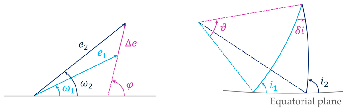
where the symbols $\delta e$ and $\phi$ represent the magnitude and phase of the relative eccentricity vector, respectively, whereas $\delta i$ and $\vartheta$ are the magnitude and phase of the relative inclination vector, as sketched in Figure 1.

Within the ROE framework, the solution to the Hill–Clohessy–Wiltshire equations (HCW) can be formulated thanks to the following transformation between the ROEs and Cartesian states [13,26]:

$$\left\{\begin{array}{c}x\left(u\right)=-a_c\hspace{0.17em}\delta e\hspace{0.17em}\cos \left(u-\phi \right)\\ y\left(u\right)=a_c\delta {\mathcal{l}}_0+2\hspace{0.17em}{a}_c\hspace{0.17em}\delta e\hspace{0.17em}\sin \left(u-\phi \right)\\ z\left(u\right)=a_c\hspace{0.17em}\delta i\hspace{0.17em}\sin \left(u-\vartheta \right)\end{array}\right.$$

(4)

where the variables $x,y,z$ define the position of the deputy with respect to the chief in the Hill frame, which has its principal axes defined as follows:

• The x-axis points from the center of the Earth to the chief satellite’s position;
• The z-axis points in the direction of the angular momentum of the chief’s orbit;
• The y-axis completes the right-handed system.

Additionally, $u=nt$ is the mean argument of latitude of the chief, with $n$ the mean motion and $t$ the time variable; the subscript ${\left(·\right)}_0$ indicates the state at $t=u=0$.

2.1.2. Parametric Expression of the HoA

The ROEs are particularly convenient for expressing the variation in the HoA in time because of the intuitive geometric interpretation of the relative motion they provide. Indeed, by introducing a parametric expression of the HoA as a function of ROEs, the impact that the satellite dynamics has on the interferometric problem can be easily understood. Given the wavelength $\lambda$, the slant range $r_0$, the incidence angle ${\theta }_i$ and the effective baseline $B_{\perp }$, the HoA for a bistatic acquisition is defined as follows [1,2]:

$$\mathrm{H}\mathrm{o}\mathrm{A}={\displaystyle \frac{\lambda \hspace{0.17em}{r}_0\hspace{0.17em}\mathrm{s}\mathrm{i}\mathrm{n}{\theta }_i}{B_{\perp }}}.$$

(5)

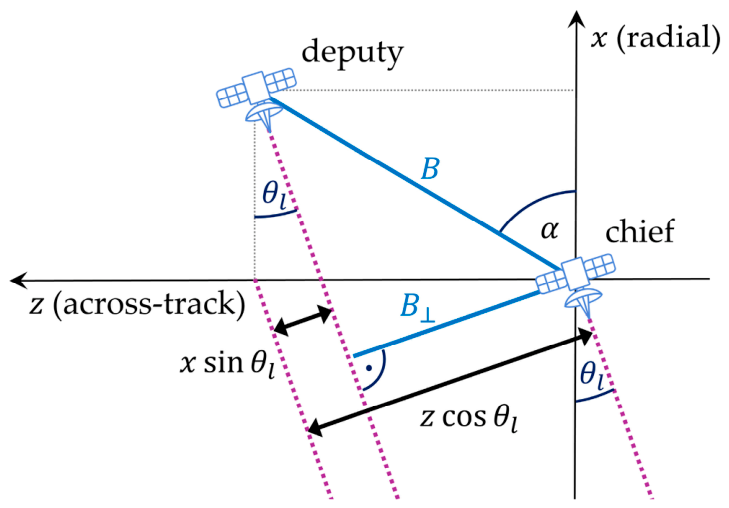
The relative geometry does not influence any of the terms at the numerator (wavelength, slant range and incidence angle), but only the effective baseline $B_{\perp }$. Accordingly with [27], the effective baseline in across-track interferometry is computed from the separation in the radial $\left(x\right)$ and across-track $\left(z\right)$ directions, projected onto the radar line of sight. As such, it nullifies when the satellites are aligned in that direction. Considering the geometry depicted in Figure 2, $B_{\perp }$ can be written as a function of the look angle ${\theta }_l$ and the angle $\alpha$ defining the relative position of the two satellites [27]:

$$\begin{array}{r}{B}_{\perp }\left({\theta }_l,u\right)=\left|B\left(u\right)\cdot \left(\mathrm{s}\mathrm{i}\mathrm{n}\left(\alpha -{\theta }_l\right)\right)\right|=\\ =\left|B\left(u\right)\cdot \left(\mathrm{s}\mathrm{i}\mathrm{n}\alpha \mathrm{c}\mathrm{o}\mathrm{s}{\theta }_l-\mathrm{c}\mathrm{o}\mathrm{s}\alpha \mathrm{s}\mathrm{i}\mathrm{n}{\theta }_l\right)\right|=\\ =\left|-x\left(u\right)\mathrm{s}\mathrm{i}\mathrm{n}{\theta }_l+z\left(u\right)\mathrm{c}\mathrm{o}\mathrm{s}{\theta }_l\right|.\end{array}$$

(6)

Notably, the mean argument of latitude $u$ is the only time-dependent parameter. To express the effective baseline in terms of the ROEs, the mapping connecting them to the coordinates in the Hill frame for a harmonic solution of the HCW in Equation (4) can be employed. Considering relative orbits bounded and centered with respect to the chief (i.e., $\delta a=\delta {\mathcal{l}}_0=0$ in absence of perturbations) and employing the amplitude/phase form of the eccentricity and inclination vectors, the effective baseline reads:

$$B_{\perp }=\left|-a_c\delta e\mathrm{c}\mathrm{o}\mathrm{s}\left(u-\phi \right)\mathrm{s}\mathrm{i}\mathrm{n}{\theta }_l+a_c\delta i\mathrm{s}\mathrm{i}\mathrm{n}\left(u-\vartheta \right)\mathrm{c}\mathrm{o}\mathrm{s}{\theta }_l\right|.$$

(7)

Finally, substituting the last expression into the definition of the HoA in Equation (5), the parametric formula of the HoA is found analogously as in [28], where it has been exploited to optimize the incidence angle in a single-baseline scenario:

$$\mathrm{H}\mathrm{o}\mathrm{A}={\displaystyle \frac{\lambda \hspace{0.17em}{r}_0\mathrm{s}\mathrm{i}\mathrm{n}{\theta }_i}{a_c\left|\delta e\mathrm{c}\mathrm{o}\mathrm{s}\left(u-\phi \right)\mathrm{s}\mathrm{i}\mathrm{n}{\theta }_l+\delta i\mathrm{s}\mathrm{i}\mathrm{n}\left(u-\vartheta \right)\mathrm{c}\mathrm{o}\mathrm{s}{\theta }_l\right|}}.$$

(8)

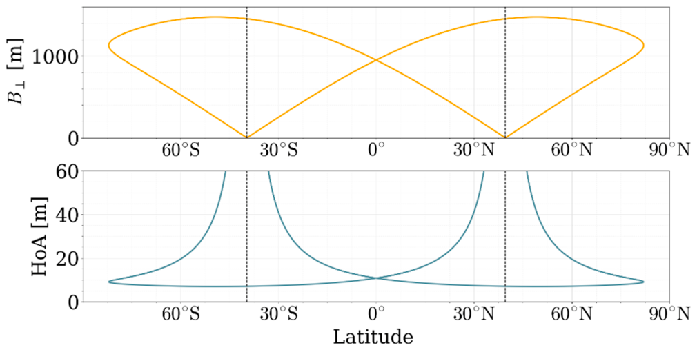
The expression in Equation (8) links the HoA directly to the orbital geometry, making it possible to design formations with predictable DEM accuracy. Another advantage is that it confines the variation in the HoA due to the elapsed time in the mean argument of latitude only, while the dependence on the ROEs is determined by the parameters $\delta e, \delta i,\phi ,\vartheta$. Moreover, it highlights the $\pi$-periodicity exhibited by the HoA relative to the mean argument of latitude. Finally, it implies that the HoA is not defined for every value of $u$, but instead tends to an asymptote at latitudes corresponding to a null effective baseline. Figure 3 shows the effective baseline and the HoA as a function of the latitude for a satellite pair flying in a sun-synchronous orbit (SSO), a widely employed solution for missions requiring homogeneous illumination over time, achieved with a slightly tilted orbit with respect to a perfectly polar one, where the latitudes near the polar caps are not covered (please note that high-latitudes values are missing in Figure 3).

The expression in Equation (6) considers the effective baseline with its across-track and radial components. However, although being particularly favorable from the computational point of view, this assumption is not always applicable, especially in configurations with a non-negligible along-track separation, i.e., a few hundred meters. This is because the Earth’s rotation introduces a coupling between the along-track and the across-track separations, which would add a degree of freedom to the optimization problem: namely the along-track separation or, equivalently, the mean argument of longitude $\delta \mathcal{l}$ [29,30]. The coupling would make the analytical treatment of the problem much more complicated; for this reason, we will initially consider the formula in Equation (6) for the effective baseline in the analytical derivation, and then, in Section 3.2.3, we analyze the effect of the Earth’s rotation on the obtained solution.

2.1.3. Generalized Helix Formation

The mapping between the ROEs and the HoA derived in Equation (8) shows that the time evolution of the HoA is uniquely determined by the magnitudes and phases of the relative eccentricity and inclination vectors. However, not all combinations of these parameters are operationally feasible, since collision avoidance is not guaranteed a priori. For example, as shown in [13], an additional constraint on the relative eccentricity and inclination vectors can be imposed to achieve passive safety, leading to the classical helix formation in the two-satellite case:

$$\vartheta =\phi +n\pi , n\in \mathbb{Z}$$

(9)

The practical utility of the helix lies in allowing maximization of the minimum distance in the x–z plane of the Hill frame, given the magnitudes of the relative eccentricity and inclination vectors, through the imposition of a phase relationship on the chief-referenced ROEs. The generalization of this concept to a constellation of $N$ satellites is introduced in the following, with the objective of establishing a helix in which analogous conditions hold for each possible pair of satellites in the formation. To do so, we consider the differences between the eccentricity and inclination vectors of the $(N-1)$ deputies (expressed as pairwise differentials):

$$\left\{\begin{array}{c}\Delta {\mathbf{e}}_{i,j}=\Delta {\mathbf{e}}_i-\Delta {\mathbf{e}}_j=\left[\begin{array}{c}\delta e_i\mathrm{c}\mathrm{o}\mathrm{s}\left({\phi }_i\right)-\delta e_j\mathrm{c}\mathrm{o}\mathrm{s}\left({\phi }_j\right)\\ \delta e_i\mathrm{s}\mathrm{i}\mathrm{n}\left({\phi }_i\right)-\delta e_j\mathrm{s}\mathrm{i}\mathrm{n}\left({\phi }_j\right)\end{array}\right]\\ \Delta {\mathbf{i}}_{i,j}=\Delta {\mathbf{i}}_i-\Delta {\mathbf{i}}_j=\left[\begin{array}{c}\delta i_i\mathrm{c}\mathrm{o}\mathrm{s}\left({\phi }_i+n\pi \right)-\delta i_j\mathrm{c}\mathrm{o}\mathrm{s}\left({\phi }_j+m\pi \right)\\ \delta i_i\mathrm{s}\mathrm{i}\mathrm{n}\left({\phi }_i+n\pi \right)-\delta i_j\mathrm{s}\mathrm{i}\mathrm{n}\left({\phi }_j+m\pi \right)\end{array}\right]\end{array}\right.$$

(10)

where the subscripts $i,j$ ($i\ne j$) denote distinct deputies and $n$ and $m$ are integers. According to [13], all vector pairs must be (anti-)parallel for each couple of satellites to ensure mutual passive safety. This can be equivalently expressed by equating their cross-product to zero:

$$\Delta {\mathbf{e}}_{i,j}\times \Delta {\mathbf{i}}_{i,j}=0$$

$$\iff \left(\delta e_i\delta i_j-{\left(-1\right)}^{n-m} \delta e_j\delta i_i\right)\cdot \mathrm{s}\mathrm{i}\mathrm{n}\left({\phi }_i-{\phi }_j\right)=0$$

(11)

A dedicated analysis of the compliance of the passive-safety constraint in Equation (11) with the optimized configurations is provided in Section 3.3.

Equation (11) indicates that it is in fact possible to obtain a generalized helix under two possible necessary conditions (in addition to the aforementioned conditions on $\delta a$ and minimum magnitudes $\delta e$ and $\delta i$):

• Common orientation of the eccentricity vectors. All the eccentricity vectors are collinear:

$${\phi }_i={\phi }_j+k\pi \hspace{0.33em}\forall \hspace{0.17em}i,j; k\in \mathbb{Z}$$

(12)

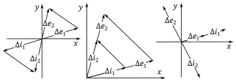
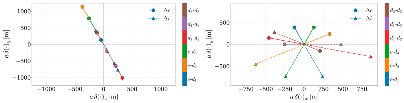
If we combine Equation (12) with the definition of helix, all the relative eccentricity and inclination vectors for each pair must lie on the same line. An example of a possible configuration of the vectors $\Delta \mathbf{e}$ and $\Delta \mathbf{i}$ for each satellite’s pair falling in this category is illustrated in the left panel of Figure 4. The circular and triangular markers indicate the relative eccentricity and inclination vectors, respectively, for each pair of satellites in the formation. Please note that for an $N$-satellite formation there are $\left(N\right(N-1)/2)$ possible pairs; the configuration in Figure 4 displays all the six relative eccentricity and inclination vectors of a four-satellite formation. As required by the first category of passively safe configurations (i.e., compliant with Equation (12)), these vectors all lie on the same line. After the enforcement of this constraint, the remaining design variables are:

-

The magnitudes of the relative eccentricity and inclination for all deputy spacecraft.

-

The orientation of the first deputy’s relative eccentricity and inclination.

-

The orientation of the other deputies’ relative eccentricity and inclination, which is parallel to the orientation of the first deputy.

Furthermore, deputies with identical $\Delta \mathbf{e}$ and $\Delta \mathbf{i}$ vectors are obviously not allowed; therefore, no pair of deputies may share the same magnitudes $\delta e \mathrm{a}\mathrm{n}\mathrm{d} \delta i$ if they have the same $\phi$and the same $\vartheta$ (i.e., they are defined by the same $n$ in Equation (9) and the same $k$ in Equation (12)).

2.

Same orbit shape ratio. All deputies have identical ratios between the magnitude of the relative eccentricity and the relative inclination, i.e.,

$$\delta e_i/\delta i_i={\left(-1\right)}^{n-m}\delta e_j/\delta i_j\hspace{0.33em}\forall i,j$$

(13)

In other words, all relative orbits must be scaled versions of each other. The right panel of Figure 4 displays an exemplary configuration for this second category of generalized helix. Again, note that the vectors representing the relative eccentricity (circular markers) and relative inclination (triangular markers) are collinear for every pair of satellites. Additionally, in this second category of passively safe configurations, the ratio of the lengths of the vectors $\Delta \mathbf{e}$ and $\Delta \mathbf{i}$ is constant. Therefore, the remaining design variables are:

-

The orientations of the relative eccentricity and inclination for all deputy spacecraft.

-

The magnitude of the first deputy’s relative eccentricity and inclination.

-

The magnitude of the other deputies’ relative eccentricity, whereas that of the relative inclination is fixed by Equation (13).

The passive-safety constraint defined in Equation (13) can be met only if the quantity $(n-m)$ is even. Converting this condition to the mutual orientation of the $\left(\Delta {\mathbf{e}}_{i,j},\hspace{0.33em}\Delta {\mathbf{i}}_{i,j}\right)$ vectors of all deputy pairs, it means that they can all only have the same direction, or all in opposite directions, i.e., all deputies’ ROEs must share the same constant $n$ in Equation (9). For example, in the case reported in Figure 4, the relative inclination vector always points in the opposite direction from the relative eccentricity vector for each pair. This rule is in agreement with the simple geometric considerations illustrated in the three qualitative plots of Figure 5: in the left and central plots, the vector differences between the relative eccentricity and inclination vectors of two chief–deputy pairs can be (anti-)parallel, while this is not possible in the right plot, where one pair has vectors pointing in the same direction, with the other pair in opposite directions. Note that Figure 5 is not providing any quantitative results, but just illustrating the geometrical interpretation of the $(n-m)$ term in Equation (13).

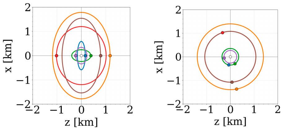
Figure 6 shows two practical implementations of the generalized helix concept for both the identified passive-safety conditions applied to a four-satellite formation. Here, the relative orbits between all six possible satellite pairs are projected on the x–z plane of the Hill frame (i.e., with the $x$ coordinate indicating the vertical direction and for $z$ the across-track direction) centered on one of the two satellites of the pair. The markers indicate the relative positions of the satellites at the equator, i.e., when the mean argument of latitude is null. By observing Figure 6, and especially the plot on the left, one may get the impression that there is an unsafe intersection of the relative trajectories. However, not only is this prevented by Equations (12) and (13), but because all six relative trajectories are displayed in the figure, the unsafe condition would be met only if one of the orbits intersects with the origin of the reference frame, which clearly does not happen. In the left plot the formation is such that the $\Delta \mathbf{e}$ and $\Delta \mathbf{i}$ vectors lie on the same line under the specific condition $\phi =\vartheta =\pi /2+k\pi ,k\in \mathbb{Z}$. This is highlighted by the reported initial positions of the satellites, located at an angular distance of $\pm \pi /2$ from the x-axis. The right plot, instead, reports a configuration in which the x–z-projected orbits are scaled versions of each other in the particular case with $\delta e_i/\delta i_i=1$: we will refer to this geometry as projected circular orbit (or xz-PCO) hereafter [27].

2.2. Mathematical Formulation of the Optimization Problem

Having assessed the performance metric and safety constraints, the formation design can be addressed as an optimization problem, which we will assess in terms of a generic set of ROEs to then verify whether the solution complies with the passive-safety requirements defined in Section 2.1.3. We first consider a simplified two-satellite scenario to gain an analytical insight, and then extend the formulation to multi-satellite, multi-baseline configurations, where multiple interferograms are available within the same pass. In the following, it is considered that the formation acquires images with a fixed angle of incidence ${\theta }_i$ at each latitude. An analysis on the ideal way to set the incidence angle as a function of the latitude to ensure the uniformity of the DEM has been explored in [28]. The optimization problem is first formulated in the two-satellite case in Section 2.2.1, allowing for a purely analytical solution, and subsequently generalized to the $N$-satellite case in Section 2.2.2. Further remarks on the properties of the optimization problem are provided in Section 2.2.3.

2.2.1. Single-Baseline Problem

The problem is formulated for a single pair of satellites in the following. The aim is to keep the HoA as expressed in Equation (8) as close as possible to a desired nominal value ${\mathrm{HoA}}^{\ast }.$ This is expressed by minimizing an $L_2$-type functional over a set $\mathcal{U}$ of mean arguments of latitude of the chief satellite $u$:

$$\begin{array}{c}\mathrm{a}\mathrm{r}\mathrm{g}\underset{\delta \mathsf{\alpha }}{\mathrm{m}\mathrm{i}\mathrm{n}}J:={\int }_{\mathcal{U}}{\left(\mathrm{HoA}\left(\delta \mathsf{\alpha },u\right)-{\mathrm{HoA}}^{\ast }\right)}^2\hspace{0.17em}du=\\ ={\int }_{\mathcal{U}}{\left({\displaystyle \frac{K}{a_c\left|\delta e \mathrm{c}\mathrm{o}\mathrm{s}\left(u-\phi \right)\mathrm{s}\mathrm{i}\mathrm{n}{\theta }_l+\delta i \mathrm{s}\mathrm{i}\mathrm{n}\left(u-\phi +n\pi \right)\mathrm{c}\mathrm{o}\mathrm{s}{\theta }_l\right|}}-{\mathrm{HoA}}^{\ast }\right)}^2\hspace{0.17em}du,\end{array}$$

(14)

where the coefficient $K={\displaystyle \frac{\lambda r_0\mathrm{s}\mathrm{i}\mathrm{n}{\theta }_i}{a_c}}$, embedding all the constant parameters that are introduced, and we recall that $\vartheta =\phi +n\pi$.

Because the HoA inherits a $\pi$-periodicity in $u$ (through the effective baseline), the same result obtained over a full orbit can be recovered over a half-period interval. However, the HoA is not defined for every $u$: it tends to an asymptote at latitudes where the effective baseline nullifies, and this makes the integral diverge if $\mathcal{U}$ spans an interval wider than half a period. When the optimization is carried out over a full $\pi$-wide interval (or equivalently over a full period of the HoA), latitudes close to the asymptote must be excluded to keep the objective well-defined. This is achieved by multiplying the integrand by a suitable window that removes a neighborhood of the asymptote

$$w_{rect}\left(u\right)=\left\{\begin{array}{c}0 \mathrm{i}\mathrm{f} \left|u-u_a\right|<\epsilon \\ 1 \mathrm{e}\mathrm{l}\mathrm{s}\mathrm{e}\mathrm{w}\mathrm{h}\mathrm{e}\mathrm{r}\mathrm{e}\end{array}\right.$$

(15)

where $u_a$ is the asymptote location, while the parameter $\epsilon$ can be imposed to tune the latitudes considered in the optimization. Therefore, the windowed cost functional becomes:

$$J={\int }_{\mathcal{U}}{w}_{rect}\left(u\right) {\left({\displaystyle \frac{K}{a_c\left|\delta e \mathrm{c}\mathrm{o}\mathrm{s}\left(u-\phi \right)\mathrm{s}\mathrm{i}\mathrm{n}\left({\theta }_l\right)+{(-1)}^n\delta i\mathrm{s}\mathrm{i}\mathrm{n}\left(u-\phi \right)\mathrm{c}\mathrm{o}\mathrm{s}\left({\theta }_l\right)\right|}}-{\mathrm{H}\mathrm{o}\mathrm{A}}^{\ast }\right)}^{2}du.$$

(16)

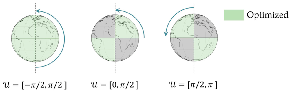
For global coverage, the interval $u\in [0,\pi ]$ is not strictly required. Because of $\pi$-periodicity, it is sufficient to use $u\in [0,\pi /2]$ (corresponding to $\epsilon = \pi /4$) so that each latitude is acquired once (e.g., the Northern Hemisphere on the ascending arc and the Southern Hemisphere on the descending arc). A sketch of such an acquisition strategy is given in Figure 7. Restricting the integration interval to $u\in [0,\pi /2]$ avoids divergence without windows but introduces a dependence on the phase angles: over a full period, the periodicity makes phase shifts irrelevant, whereas over a shorter interval the alignment of the function HoA$\left(u\right)$ with respect to $\mathcal{U}$ becomes relevant. Notably, the optimization problem in Equation (14) is solvable analytically under the hypothesis $u\in [0,\pi /2]$: its solution is reported in Section 3.1. For the single-baseline case, an optimization of the helix formation has been very recently devised for ESA’s Harmony mission and described in [17].

2.2.2. Multi-Baseline Problem

The single-baseline scenario allows for determining the set of ideal configurations to maintain a nominal HoA with a two-satellite formation. The aim of this work, however, is to also investigate the improvement that a larger number of satellites—and thus more baselines—can bring. Extending the problem setup of the single-baseline scenario, two nominal, target values for the HoA are considered: ${\mathrm{H}\mathrm{o}\mathrm{A}}_1^{\ast }$ and ${\mathrm{H}\mathrm{o}\mathrm{A}}_2^{\ast }$. To simultaneously be sufficiently close to both of them, we formulate a multi-objective optimization problem where the objective functions are given by the $L_2$ distances from the target HoAs, and the decision variables are the ROEs of the satellite formation (no safety requirement is imposed here, but the compliance of the solutions with the passive-safety conditions defined in Section 2.1.3 is discussed later in Section 3.3). For a more practical formalization it is convenient to define the set of deputies $\mathcal{D}$ and the set of satellite pairs $\mathcal{P}$ (if a formation is made of $N$ real satellites with one of them being the chief and $(N-1)$ the deputies; $\mathcal{D}$ has cardinality $\left|\mathcal{D}\right|=N-1$, while $\left|\mathcal{P}\right|=N\left(N-1\right)/2$). Additionally, $\delta {\mathsf{\alpha }}_d$ is used to indicate the set of relative orbital elements of the $d$-th deputy with respect to the chief, whereas ${\mathrm{H}\mathrm{o}\mathrm{A}}_p$ is defined as the height of ambiguity given by the $p$-th satellite pair. Moreover, it is assumed that for each value of the mean argument of latitude of the satellite that serves as the chief, the images acquired by any pair of satellites can be combined to form an interferogram. The multi-objective optimization reads:

$$\arg \underset{\delta {\mathsf{\alpha }}_d,d\in \mathcal{D}}{\mathrm{m}\mathrm{i}\mathrm{n}}(F_1(\delta {\mathsf{\alpha }}_d), F_2(\delta {\mathsf{\alpha }}_d))$$

(17)

where the objective functions are defined as follows:

$$F_i={\int }_{\mathcal{U}}\underset{p\in \mathcal{P}}{\mathrm{m}\mathrm{i}\mathrm{n}}{\left({\mathrm{H}\mathrm{o}\mathrm{A}}_p\left(\delta {\mathsf{\alpha }}_d,\hspace{0.17em}u\right)-{\mathrm{H}\mathrm{o}\mathrm{A}}_i^{\ast }\right)}^2\hspace{0.17em}du.$$

(18)

The idea is to select the baseline closest to achieving the desired HoA among those available at each mean argument of latitude via the min operator in Equation (18), which is then integrated over all the mean argument of latitudes overflown by the chief satellite. The best combination of ROEs to minimize the root mean square errors $F_1$ and $F_2$ with respect to $\mathrm{H}\mathrm{o}{\mathrm{A}}_1^{\ast }$ and $\mathrm{H}\mathrm{o}{\mathrm{A}}_2^{\ast }$, respectively, is then determined within Equation (17), which gives the solution of the multi-objective optimization in the ROE space.

To reduce the multi-objective formulation to a single cost function, thus easing the computations, we introduce a weighted-sum scalarization:

$$\left\{\begin{array}{c}J=w_1{F}_1\left(\delta {\mathsf{\alpha }}_d\right)+w_2{F}_2\left(\delta {\mathsf{\alpha }}_d\right)\hspace{0.17em}, w\ge 0\\ w_1+w_2=1\end{array}\right.$$

(19)

The choice of the coefficients $w_1,w_2$allows us to give more importance to either of the two objectives and, by making them vary in the interval [0, 1], it is possible to obtain (part of) the Paretian solutions. Although different combinations of weights have been tested, the results shown in Section 3 have been obtained by adopting the weights:

$$w_i={\displaystyle \frac{1/{\mathrm{H}\mathrm{o}\mathrm{A}}_i^{\ast }}{{\displaystyle {\sum }_{j=1}^2}{1/\mathrm{H}\mathrm{o}\mathrm{A}}_j^{\ast }}}, i=1, 2.$$

(20)

This choice is motivated by the need to attribute the same importance to the relative errors with respect to each of the nominal HoA, leading to an impartial balance between the two objectives.

To improve the computational efficiency and ease coupling with passive-safety constraints, the optimization is not performed directly over each deputy’s ROE components. Instead, each chief–deputy baseline is parameterized in amplitude–phase form (maximum effective baseline and phase shift), yielding a compact set of non-redundant decision variables: the solution to the optimization is therefore determined in terms of the maximum effective baselines $B_{\perp max,j}$, which provides information about the size of the relative orbit; ${\delta }_1$, the angular position of the first deputy along its orbit relative to the chief; and ${\delta }_{1,j}$, the angular separation between the first baseline and all the others. Mathematically, these quantities are defined as follows:

$$B_{\perp j}\left(u\right)=B_{\perp max,j}\left|\cos (u-{\delta }_j)\right|$$

(21)

$$\left\{\begin{array}{c}{B}_{\perp max,j}=\sqrt{{\delta e}_j^2{\mathrm{s}\mathrm{i}\mathrm{n}}^2{\theta }_l+{\delta i}_j^2{\mathrm{c}\mathrm{o}\mathrm{s}}^2{\theta }_l}\\ {\delta }_j={\phi }_j+{\left(-1\right)}^n\arctan \left({\displaystyle \frac{\delta e_j}{\delta i_j}}\tan {\theta }_l\right)\end{array}\right.$$

(22)

The problem size for a formation of $N$ satellites is hence reduced from $3\cdot \left(N-1\right)$ to $2\cdot \left(N-1\right)$ non-redundant decision variables.

2.2.3. Remarks on the Optimization Problem

The properties of the optimization problem defined in Equations (17) and (18) are further discussed in this section, as they are fundamental to the choice of the solution method.

By virtue of the amplitude–phase parametrization of Equations (21) and (22), the feasible set is defined in ${\mathbb{R}}^{2(N-1)}$, and no further constraints are imposed. Indeed, although the passive-safety conditions, illustrated in Section 2.1.3, are not considered here, they will be shown to be compatible with the optimal solution up to one degree of freedom in Section 3.3. Furthermore, all baselines are in the form given in Equation (21), i.e., harmonics whose magnitude and phase are determined by the decision variables $B_{\perp max,j}$ and ${\delta }_{1,j}$. This follows from the fact that the coordinates of the distance vector between the satellites are harmonic, as a consequence of their harmonic relative motion with respect to the mean argument of latitude in Equation (4). The objective in Equation (18) depends on $\left|\mathcal{P}\right|=N\left(N-1\right)/2$ pairs, whose $2\left|\mathcal{P}\right|$ amplitudes and phases are generated by only $2(N-1)$ free parameters. Consequently, the pairwise baselines are not independent: this means that the deputy–deputy baselines cannot be placed freely, which motivates the limitation of the heuristic proposed in Section 2.3.1 and its subsequent refinement in Section 2.3.2. Concerning the well-posedness of the problem, please note that in the single-baseline case, this required the windowing function in Equation (15) to prevent the objective from diverging. In the multi-baseline case instead, the min operator in Equation (18) completely removes the issue. Indeed, the innermost term selects at any mean argument of latitude the pair closest to the target, making the integrand always bounded, as long as the baselines do not vanish simultaneously. Hence, the objective is always finite with the exception of this degenerate set, where the integral diverges, but this is not an issue due to the presence of the min operator. Additionally, the integrand is continuous, as it is a minimum of finitely many continuous functions; $F_i$ is therefore continuous, from which it follows the existence of a minimizer on the compact feasible set. The objective is not differentiable, if the argument of the minimum in Equation (18) is not unique, which happens when the heights of ambiguity provided by two pairs are equidistant from the given target. It is not convex either: in general, a minimum of convex functions is non-convex, and the uniqueness of the minimizer is not guaranteed. Note that part of the non-uniqueness can be readily interpreted, in that it reflects the invariance of the formation to relabeling, which produces differently named although physically equivalent parametrizations of the same formation.

2.3. Methodologies for the Solution of the Multi-Objective Optimization Problem

This section presents the methodologies employed to solve the multi-baseline problem described in Equation (17). First, a heuristic strategy is introduced in Section 2.3.1, leveraging the result obtained for the two-satellite problem. The solution is subsequently refined numerically exploiting genetic algorithms, as illustrated in Section 2.3.2.

2.3.1. Heuristic Approach

The presence of the min operator in the objective function in Equation (17), and the absolute values in the HoA definition in Equation (8) do not allow for the analytical determination of the gradient of the objective and, in general, make it difficult to solve the problem using gradient-based methods [31]. Therefore, an approximate solution based on the exact result obtained for a two-satellite formation is initially provided. The logical procedure followed to obtain the heuristic solution is based on the following five steps:

• In a formation consisting of a chief c and two deputies $d_1, d_2$, the two deputies are positioned so that the pairs $c-d_1,c-d_2$ minimize Equation (14) for each of the two objective values of $\mathrm{H}\mathrm{o}{\mathrm{A}}^{\ast }$.
• The relative RMSE for each of the two nominal $\mathrm{H}\mathrm{o}{\mathrm{A}}^{\ast }$s is computed.
• A new deputy $d_i$ is added to the formation so that the pair $c-d_i$ is optimized with respect to the $\mathrm{H}\mathrm{o}{\mathrm{A}}^{\ast }$ with the worst relative root mean square error (RMSE).
• If multiple pairs $c-d_j$ share the same target $\mathrm{H}\mathrm{o}{\mathrm{A}}^{\ast }$, their phases ${\phi }_j$ are recomputed so that the functions $\mathrm{H}\mathrm{o}{\mathrm{A}}_{\mathrm{j}}$ are equally spaced in the interval $u\in \left[0,\pi /2\right]$. This is done by imposing that they respectively reach the minimum HoA in correspondence with the argument of latitude $u={\delta }_j$, given by:

$${\delta }_j={\displaystyle \frac{\pi }{4N}}\left(2j-1\right).$$

(23)

5.

The procedure is iterated until a formation with the desired number of deputies is achieved.

In its essence, this algorithm ensures that all chief–deputy baselines are distributed to provide the most homogeneous coverage of the objectives. However, by definition, the proposed heuristic does not consider pairs consisting of two deputies, which represents the main drawback of using this method without subsequent refinements.

The baselines, HoAs and RMSE resulting from the proposed heuristic are presented in Section 3.2.1.

2.3.2. Numerical Approach

In order to cope with the limitations of the heuristic approach, we consider methods based on genetic algorithms, given their simplicity of implementation and their superiority over gradient-based methods in handling problems with multiple local minima. Indeed, the one in Equation (17) falls into this category: given a set of effective baselines, a local minimum is reached whenever one or more of them reaches the optimal value for a target HoA. At this point, only a complete change in the assignments of each baseline to the target values would allow for further improvement. The consequence is the introduction of multiple disconnected local minima, with respect to which we aim to obtain a low sensitivity. Furthermore, the problem has a low number of objectives (two, one for each of the target HoA) and a size (i.e., number of decision variables) that depends on the number of satellites considered, medium to low in the considered cases. Therefore, some of the most commonly used algorithms tailored to this type of problem are employed in the resolution, and a comparison of the results obtained with each of them is provided in Section 3.2.2. All experiments were conducted on a machine with an Intel^® Core™ Ultra 7 165H (16 cores, 22 Threads, 3.8 GHz), 32 GB RAM, and running Windows 11 (64-bit). The code was implemented in Python 3.12.3 with Pygmo 2.19.7. The random seed used for the initialization of the SaDE+Compass algorithm is: 123456789. The considered algorithms are:

• Covariance Matrix Adaptation Evolution Strategy (CMA-ES). This is one of the most well-established and first evolution strategy algorithms to be developed, considered as the benchmark against which the others are compared [32].
• Self-adaptive Differential Evolution (SaDE). This algorithm dynamically adapts its control parameters (mutation and crossover strategies) during the run, thus removing the need for manual fine-tuning [33].
• Artificial Bee Colony (ABC). Its main advantage is the lower sensitivity to local minima. However, it generally provides slower convergence than the others [34].

After having performed the global search employing either one of those three, a further refinement of the solution is achieved by employing the local Compass Search algorithm [35]. The baselines, HoA, and RMSE resulting from the numerical optimization are reported in Section 3.2.2, along with two examples of optimal configurations compliant with the safety requirements defined in Section 2.1.3.

2.4. Formation Maintenance Background

Once the optimal formations have been identified according to the procedure illustrated in Section 2.3, and the passive safety according to the requirements in Section 2.1.3 has been ensured (see Section 3.3), the most desirable formations are those that also allow fuel saving. We therefore assess formation-keeping costs in the LEO environment by estimating the required $\Delta \mathrm{v}$ under representative disturbance models and impulsive control strategies. Perturbations modify both the magnitudes and, crucially, the relative phases of the satellite pairs that determine the HoA evolution. In particular, the angular shifts that distribute HoA minima over the imaging interval tend to drift, producing a progressive mismatch between the achieved HoA and the nominal target values, as better detailed in Section 2.4.1. The degradation can be quantified by the same RMSE metric adopted in the optimization, computed over the acquisition interval.

Therefore, this section presents the context and the methodologies employed to derive a coarse estimate of the control effort required for the formation maintenance of the scientific optimal and passively safe formations identified. To this end, the employed model of the orbital disturbances is described in Section 2.4.1. The impulsive control strategies adopted for the formation-keeping modeling are illustrated in Section 2.4.2.

2.4.1. Orbital Disturbances’ Model

A first-order estimate of formation-keeping costs is obtained by propagating candidate formations under the first zonal harmonic of the geopotential ($J_2$) and differential atmospheric drag, and by computing the impulsive $\Delta \mathrm{v}$ required to restore the nominal ROEs. To provide an estimate of the formation maintenance cost, the representative scenario in

Table 1. Orbital and interferometric reference parameters.

Parameter	Value
Orbit type	SSO with inclination ≈ 97.5°
Formation categories	xz-PCO, Helix
N° satellites	3, 4
Altitude range	[500 km, 580 km]
Atmosphere density	[1, 5]·10−12 kg/m3
CB	0.021 [m2/kg]
ΔCB	[0%, 50%] · CB
Orbital tube diameter	250 m
Baseline range	≈[200 m, 2000 m]
Incidence angle	37.0°
Look angle	33.8°
Wavelength	0.031 m (X-band)
Nominal HoAs	{10 m, 30 m}

is considered, where all the parameters are selected taking those of TanDEM-X as a reference. Specifically, the average air density $\overline{\rho }$ is computed from the exponential model of the atmosphere [36]:

$$\rho \left(h+\Delta h\right)=\rho \left(h\right)e^{-h/H}$$

(24)

where $h$ is the height and $H$ the height scale, which depends on the intensity of the solar activity. Considering a scale height of 50 km as a mid-range value under moderate solar activity and a reference altitude of 500 km, the density change across a few hundred meters (compatible with the size of TanDEM-X orbital tube) is small, and thus a constant density approximation is retained as reasonable for a first-order estimate of the formation-keeping cost [37].

For the acceleration induced by $J_2$, the relative acceleration components are evaluated directly in the Hill frame via a closed-form expression from [38]:

$$\left[\begin{array}{c}{a}_R^{J2}\\ a_T^{J2}\\ a_N^{J2}\end{array}\right]=\Gamma \left[\begin{array}{ccc}12{\mathrm{s}\mathrm{i}\mathrm{n}}^{2}i{\mathit{sin}}^{2}u-4& -4\sin 2u{\mathrm{s}\mathrm{i}\mathrm{n}}^{2}i& -4\sin u\sin 2i\\ -4\sin 2u{\mathrm{s}\mathrm{i}\mathrm{n}}^{2}i& \left(7{\mathrm{c}\mathrm{o}\mathrm{s}}^{2}u-5\right){\mathrm{s}\mathrm{i}\mathrm{n}}^{2}i+1& \cos u\sin 2i\\ -4\sin u\sin 2i& \cos u\sin 2i& \left(5{\mathrm{c}\mathrm{o}\mathrm{s}}^{2}u-7\right){\mathrm{s}\mathrm{i}\mathrm{n}}^{2}i+3\end{array}\right]\left[\begin{array}{c}x\\ y\\ z\end{array}\right]$$

(25)

where $\Gamma =-{\displaystyle \frac{3{\mu }_E{J}_2{R}_E^2}{2r^5}}$, the constant $J_2$ is the second zonal harmonic coefficient of Earth’s gravitational potential, $R_E$ is the Earth’s radius equal to $6378.15 \mathrm{k}\mathrm{m}$, $r$ is the distance between the center of the Earth and the chief, and ${\mu }_E$ is the gravitational parameter of the Earth equal to $\mathrm{398,600}$ $\mathrm{k}{\mathrm{m}}^3/{\mathrm{s}}^2$. For bounded relative trajectories, the dominant secular effects due to $J_2$ on the ROEs are a change in the direction of the relative eccentricity vector in the $\left(\delta e_x,\delta e_y\right)$ plane and a change in $\delta i_y$ proportional to inclination differences: this progressively degrades both passive-safety geometry and HoA optimality unless corrected. A possible solution to avoid such a degradation is to introduce the initial condition $\vartheta =\pm \pi /2$, which eliminates the secular term in $\delta i_y$ and keeps the out-of-plane motion bounded [13].

The differential drag is modeled as a tangential-only perturbation consistent with a semi-empirical formulation for LEO formations:

$$a_T=-{\displaystyle \frac{1}{2}}{C}_B\rho ‖v_{rel}‖(v_{rel}·\widehat{T})$$

(26)

where $C_B={\displaystyle \frac{C_{d}S}{m}}$ is the ballistic coefficient, defined from the drag coefficient $C_d$; the cross-sectional area is $S$, and the mass is $m$; $\rho$ is the average air density over the maintenance interval, $v_{rel}$the spacecraft velocity relative to air, and $\widehat{T}$ the one-unit vector in the tangential direction of the Hill frame. The effect of the air drag on the whole formation (referred to as absolute drag) primarily consists of the decay of the semi-major axis and is treated separately via periodic restoration of the chief’s orbit. The $\Delta \mathrm{v}$ required for compensating this effect is approximated as [36]:

$$\Delta \mathrm{v}\approx \sqrt{{\displaystyle \frac{{\mu }_E}{r^3}}}·{\displaystyle \frac{\Delta a}{2}},$$

(27)

where $r$ is the radius of the nominal orbit, and $\Delta a$ is the semi-major axis difference to be restored. Specifically, the appropriate $\Delta \mathrm{v}$ is assumed to be provided simultaneously by all the satellites when the chief falls outside its orbital tube.

2.4.2. Impulsive Control Strategies in ROE Space

Formation-keeping cost is evaluated using impulsive maneuvers formulated in ROE space, which provides a direct link between desired corrections of the vectors $(\Delta \mathbf{e}, \Delta \mathbf{i})$ and the required $\Delta \mathrm{v}$ in the Hill frame. The mapping between an impulsive maneuver ${\left[\Delta {\mathrm{v}}_{\mathrm{x}}, \Delta {\mathrm{v}}_{\mathrm{y}}, \Delta {\mathrm{v}}_{\mathrm{z}}\right]}^T$ and the resulting ROE variation is obtained through the Gauss Variational Equations under the near-circular reference orbit assumption [39]:

$$\left\{\begin{array}{c}n{a}_c\Delta \delta a=2{\Delta \mathrm{v}}_{\mathrm{y}}\\ n{a}_c\Delta \delta \mathcal{l}=-2{\Delta \mathrm{v}}_{\mathrm{x}}\\ \begin{array}{c}n{a}_c\Delta \delta e_x={\Delta \mathrm{v}}_{\mathrm{x}}\sin u_{man}+2{\Delta \mathrm{v}}_{\mathrm{y}}\cos u_{man}\\ n{a}_c\Delta \delta e_y=-{\Delta \mathrm{v}}_{\mathrm{x}}\cos u_{man}+2{\Delta \mathrm{v}}_{\mathrm{y}}\sin u_{man}\\ \begin{array}{c}n{a}_c\Delta {\delta i}_x={\Delta \mathrm{v}}_{\mathrm{z}}\cos u_{man}\\ n{a}_c\Delta \delta i_y={\Delta \mathrm{v}}_{\mathrm{z}}\sin u_{man}\end{array}\end{array}\end{array}\right.$$

(28)

For the formation maintenance in the x–z plane, maneuvers consisting of a pair of tangential impulses are considered. This approach demonstrably requires the minimum $∆\mathrm{v}$, and the two tangential impulses are computed as [25]:

$$\left\{\begin{array}{c}\Delta {\mathrm{v}}_{\mathrm{y}1}={\displaystyle \frac{n{a}_c}{4}}\left(\delta a_{man}-\delta a\right)+\parallel \Delta {\mathbf{e}}_{man}-\Delta \mathbf{e}\parallel \\ {\Delta \mathrm{v}}_{\mathrm{y}2}={\displaystyle \frac{n{a}_c}{4}}\left(\delta a_{man}-\delta a\right)-\parallel \Delta {\mathbf{e}}_{man}-\Delta \mathbf{e}\parallel \\ u_{man}=\arctan \left({\displaystyle \frac{\delta e_{y,man}-\delta e_y}{\delta e_{x,man}-\delta e_x}}\right)\end{array}\right.$$

(29)

where $u_{man}$ is the mean argument of latitude in correspondence with the maneuver and $n$ the mean motion. Regarding the ROEs, $\Delta \mathbf{e}$ is the relative eccentricity vector, and the subscript ${\left(\cdot \right)}_{man}$ indicates the desired state after the two impulses, whereas its absence indicates the state right at the start of the maneuver.

Concerning the out-of-plane control, $\Delta \mathrm{v}$ is given by the desired variation in the relative inclination vector $\Delta \mathbf{i}$ and can be achieved by a single impulse in the out-of-plane direction [25]:

$$\left\{\begin{array}{c}\Delta {\mathrm{v}}_{\mathrm{z}1}=n\hspace{0.17em}{a}_c\parallel \Delta {\mathbf{i}}_{man}-\Delta \mathbf{i}\parallel \\ u_{N,man}=\arctan \left({\displaystyle \frac{\delta i_{y,man}-\delta i_y}{\delta i_{x,man}-\delta i_x}}\right)\end{array}\right.$$

(30)

To compensate the $J_2$-induced variations in the relative inclination vectors, out-of-plane maneuvers are used to maintain the desired $\delta i_y$ values. Given that $\delta i_x$ remains constant, impulses are applied at $u=\pi /2+k\pi , k\in \mathbb{Z}$ (i.e., at either the highest or lowest latitude), where the required $\Delta \mathrm{v}$ is minimized, to achieve the desired inclination-vector correction. Along-track separation does not directly drive interferometric performance, and radial–cross-track safety is already enforced through the minimum-distance constraints in the $x$–$z$ plane. Nevertheless, in-plane tangential maneuvers perturb the mean argument of longitude $\delta \mathcal{l}$, and navigation and thrust-direction errors can further increase along-track separation. If the along-track separation becomes too large, bistatic acquisition becomes infeasible because the satellites cannot adequately steer to image the same area. Two approaches are therefore considered for along-track maintenance:

• ${\mathcal{S}}_1$ (coupled $\mathsf{\delta }\mathrm{a}$–$\mathsf{\delta }\mathcal{l}$ management): A small non-zero difference in the semi-major axes $\delta a$ is introduced so that, with known in-plane maneuver scheduling, $\delta \mathcal{l}$ oscillates around its nominal value without diverging. This approach avoids dedicated along-track maneuvers but introduces a constant offset in the radial direction;
• ${\mathcal{S}}_2$ (threshold-triggered along-track maneuver): A dedicated along-track correction is applied once the along-track separation exceeds a prescribed threshold (e.g., 100 m in the reported representative case).

Thresholds are imposed on a minimum separation indicator and on scientific-performance degradation (via HoA RMSE), and a maneuver is performed as soon as one threshold is exceeded. For context, we also compute the $\Delta \mathrm{v}$ required to maintain time-fixed baselines, as in [24]. However, even though this strategy would allow the nominal HoA to be maintained exactly at every latitude, it would be unfeasible in the case under consideration, as it would require the use of a significantly higher $\Delta \mathrm{v}$, in the order of tens of m/s per orbital period. In fact, the inter-satellite distances considered in this representative example are up to several kilometers (derived from the HoA optimization). Such an approach would, however, be promising only when very short baselines are considered (shorter than 100 m) [24]. Section 3.4 reported the $\Delta \mathrm{v}$ spent for the relative formation maintenance in presence of the disturbances considered in Section 2.4.1.

3. Results

3.1. Solution of the Single-Baseline Optimization Problem

The single-baseline problem is the only one among those introduced in Section 2.2 that can be solved with a purely analytical approach. Solving the windowed formulation presented in Section 2.2.1, the closed-form optimum can be expressed as a locus of points in the plane of eccentricity and inclination magnitudes. In particular, the optimal set forms an ellipse in the ($\delta e,\delta i$) plane once the latitude-dependent scaling through $\sin {\theta }_l$ and $\cos {\theta }_l$is made explicit. This provides a direct design rule for interferometrically optimal formations and a metric to quantify the distance from optimality via iso-cost curves, which become scaled versions of the optimal ellipse. Therefore, the solution to the optimization problem provides the locus of points in the $\left(\delta e,\delta i\right)$ space given by:

$$\begin{array}{c}{\displaystyle \frac{\delta e^2}{{\left(\frac{K}{{\mathrm{H}\mathrm{o}\mathrm{A}}^{\ast }\mathrm{s}\mathrm{i}\mathrm{n}{\theta }_l}\frac{\mathrm{l}\mathrm{o}\mathrm{g}\left({\mathrm{t}\mathrm{a}\mathrm{n}}^2\left(\epsilon /2\right)\right)}{2\mathrm{t}\mathrm{a}\mathrm{n}\epsilon }\right)}^2}}+{\displaystyle \frac{\delta i^2}{{\left(\frac{K}{{\mathrm{H}\mathrm{o}\mathrm{A}}^{\ast }\mathrm{c}\mathrm{o}\mathrm{s}{\theta }_l}\frac{\mathrm{l}\mathrm{o}\mathrm{g}\left({\mathrm{t}\mathrm{a}\mathrm{n}}^2\left(\epsilon /2\right)\right)}{2\mathrm{t}\mathrm{a}\mathrm{n}\epsilon }\right)}^2}}=1\end{array}$$

(31)

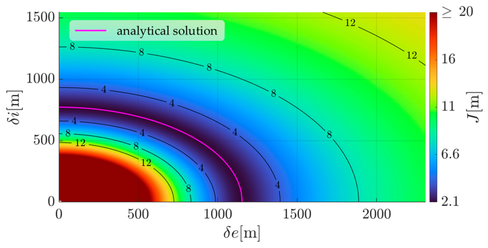
Figure 8 shows the square root of the cost function normalized by the integration interval: $\sqrt{{\displaystyle \frac{J}{\pi -2\epsilon }}}$ in the $\left(\delta e,\delta i\right)\ge 0$ quadrant given $\epsilon =\pi /4$. As expected, the resulting analytical ellipse in magenta perfectly matches the numerical minimum. The interval of mean arguments of latitude to perform the optimization to achieve global coverage is $\mathcal{U}=[0,\pi /2]$, as shown in Figure 7, Section 2.2.1. This can be conveniently achieved by requiring HoA$\left(u\right)$ to be symmetric within the interval $u\in [0,\pi /2]$. Equivalently, this imposes that the minimum of the HoA is located at $u=\pi /4$. The corresponding value of the phase of the eccentricity $\phi$ can hence be obtained by leveraging the trigonometric identity:

$$\left\{\begin{array}{c}E\sin \left(u-\phi \right)+I\cos \left(u-\phi \right)=\sqrt{E^2+I^2}\cos \left(u-\delta \right)\\ \delta =\phi +{\left(-1\right)}^n\arctan {\displaystyle \frac{E}{I}}\end{array}\right.,$$

(32)

where we imply $\vartheta = \phi +n\pi$ following the definition of a helix formation. By employing the notation

$$\left\{\begin{array}{c}E:=\delta e\sin {\theta }_l\\ \mathrm{I}:=\delta i \mathrm{c}\mathrm{o}\mathrm{s}{\theta }_l\end{array}\right.$$

(33)

and considering the expression of the $\mathrm{H}\mathrm{o}\mathrm{A}$ in Equation (8), it follows that the minimum of the function HoA(u) is obtained at $u = \delta +k\pi$, with $k$ integer. Therefore the phases must be compliant with the condition:

$$\delta = \pi /4.$$

(34)

In conclusion, substituting Equation (33) into Equation (31), the ROEs must satisfy the following condition to minimize the error between the actual and nominal $\mathrm{H}\mathrm{o}\mathrm{A}$ values globally:

$$\left\{\begin{array}{c}\sqrt{\delta e^2{\mathrm{s}\mathrm{i}\mathrm{n}}^2{\theta }_l+\delta i^2{\mathrm{c}\mathrm{o}\mathrm{s}}^2{\theta }_l}={\displaystyle \frac{2}{\mathrm{l}\mathrm{o}\mathrm{g}\left(3+2\sqrt{2}\right)}}{\displaystyle \frac{K}{{\mathrm{HoA}}^{\ast }}}\approx 1.1346{\displaystyle \frac{K}{{\mathrm{HoA}}^{\ast }}}\\ \phi +{\left(-1\right)}^n\arctan \left({\displaystyle \frac{\delta e}{\delta i\mathrm{t}\mathrm{a}\mathrm{n}{\theta }_l}}\right)={\displaystyle \frac{\pi }{4}}\end{array} \right.$$

(35)

Note that Figure 8 reports the error for the solution in Equation (35).

As a result of the optimization, two of the three decision variables $\delta e,\delta i,\phi$ ($\vartheta$ being constrained by the helix definition) are fixed, whereas the third can vary. More precisely, it is always possible to obtain the solution by arbitrarily choosing one of the two magnitudes and then solving the problem to find the other magnitude and$\phi$. However, $\phi$ cannot be set to any arbitrary value, since the arctangent operator in Equation (35) induces the presence of constraints on $\phi$, for which the following condition must hold:

$$-\pi /4<\phi <3\pi /4.$$

(36)

It is worth remarking that the presented method and the solutions illustrated hereafter refer to the global optimization (i.e., considering all latitudes the satellites overfly); nevertheless, it could be readily adjusted to target-specific regions via an appropriate tuning of the $\mathcal{U}$ set.

3.2. Solution of the Multi-Objective Optimization Problem

In this section we present the solutions to the optimization problem with both the heuristic and numerical approaches. Moreover, we also show the results following the optimization considering the coupling effect of Earth’s rotation between the along-track and across-track satellite separations.

3.2.1. Heuristic Solution

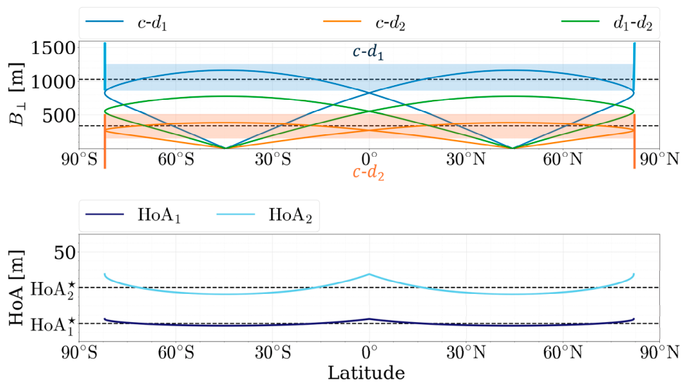
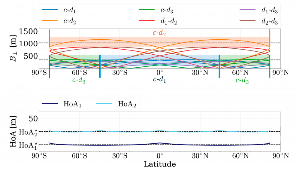
The baselines maintained at each latitude and the corresponding selected HoAs obtained by solving the optimization problem with the heuristic illustrated in Section 2.3.1 are displayed in Figure 9 and Figure 10 for three- and four-satellite formations, respectively. An example of a ROE set allowing for the achieved results in Figure 9 and Figure 10 is reported in

Table 2. Example of ROEs for heuristically optimized, passively safe, three-satellite formation.

ROE	Deputy 1	Deputy 2
$a_c\delta e$	1160 m	386 m
$\phi$	348.8°	348.8°
$a_c\delta i$	1160 m	386 m
$\vartheta$	168.8°	168.8°

and

Table 3. Example of ROEs for heuristically optimized, passively safe, four-satellite formation.

ROE	Deputy 1	Deputy 2	Deputy 3
$a_c\delta e$	350 m	1160 m	350 m
$\phi$	326.3°	348.8°	11.3°
$a_c\delta i$	350 m	1160 m	350 m
$\vartheta$	326.3°	348.8°	11.3°

, respectively. As detailed in Section 2.3, the objective is to produce two interferograms with HoAs close to the nominal values indicated by the dashed lines in Figure 9 and Figure 10, where the illustrative target values $\mathrm{H}\mathrm{o}{\mathrm{A}}_1^{\ast }=10 \mathrm{m} \mathrm{a}\mathrm{n}\mathrm{d} \mathrm{H}\mathrm{o}{\mathrm{A}}_2^{\ast }=30 \mathrm{m}$ have been assumed. In particular, the top panels show all the baselines obtained as a function of latitude. The colored areas correspond to the use of a given pair of satellites to cover the desired baseline for a range of latitudes. The underlying idea is that, for each latitude range, the best pair of satellites is chosen to create an interferogram with a HoA as close as possible to the desired one. The result in terms of HoA is then shown in the lower panels, where the HoAs of the interferograms obtained using the baselines indicated by the color pattern at each latitude are displayed. The results have been obtained considering an SSO, as it is common for remote sensing applications. Considering the altitude of TanDEM-X, such an orbit is obtained with an inclination of ≈97.5°. As a consequence, the geocentric latitude reported on the x-axis is defined in the interval ≈ [8°, 82°]. The effective baselines obtained for different target HoAs and corresponding RMSE are listed in

Table 4. Results from the heuristic optimization for a three-satellite formation.

$\mathbf{H}\mathbf{o}{\mathbf{A}}_1:\mathbf{H}\mathbf{o}{\mathbf{A}}_2\left[\mathbf{m}\right]$	${\mathit{B}}_{\perp ,\mathit{m}\mathit{a}\mathit{x}}^{\mathit{c}-{\mathit{d}}_1}\left[\mathbf{m}\right]$	${\mathit{B}}_{\perp ,\mathit{m}\mathit{a}\mathit{x}}^{\mathit{c}-{\mathit{d}}_2}\left[\mathbf{m}\right]$	${\mathit{B}}_{\perp ,\mathit{m}\mathit{a}\mathit{x}}^{{\mathit{d}}_1-{\mathit{d}}_2}\left[\mathbf{m}\right]$	$\mathbf{R}\mathbf{M}\mathbf{S}\mathbf{E}\left(\mathbf{H}\mathbf{o}{\mathbf{A}}_1\right)$ $\left[\mathbf{\%}\right]$	$\mathbf{R}\mathbf{M}\mathbf{S}\mathbf{E}\left(\mathbf{H}\mathbf{o}{\mathbf{A}}_2\right)$ $\left[\mathbf{\%}\right]$
$10:20$	$1166.6$	$583.3$	$583.3$	$10.4$	$10.4$
$10:3$0	$1166.6$	$388.8$	$777.7$	$10.4$	$10.4$
$10:40$	$1166.6$	$291.6$	$874.9$	$10.4$	$10.4$
$10:50$	$1166.6$	$233.3$	$933.3$	$10.2$	$10.4$

and

Table 5. Results from the heuristic optimization for a four-satellite formation.

$\mathbf{H}\mathbf{o}{\mathbf{A}}_1:\mathbf{H}\mathbf{o}{\mathbf{A}}_2\left[\mathbf{m}\right]$	${\mathit{B}}_{\perp ,\mathit{m}\mathit{a}\mathit{x}}^{\mathit{c}-{\mathit{d}}_1}\left[\mathbf{m}\right]$	${\mathit{B}}_{\perp ,\mathit{m}\mathit{a}\mathit{x}}^{\mathit{c}-{\mathit{d}}_2}\left[\mathbf{m}\right]$	${\mathit{B}}_{\perp ,\mathit{m}\mathit{a}\mathit{x}}^{\mathit{c}-{\mathit{d}}_3}\left[\mathbf{m}\right]$	${\mathit{B}}_{\perp ,\mathit{m}\mathit{a}\mathit{x}}^{{\mathit{d}}_1-{\mathit{d}}_2}\left[\mathbf{m}\right]$	${\mathit{B}}_{\perp ,\mathit{m}\mathit{a}\mathit{x}}^{{\mathit{d}}_1-{\mathit{d}}_3}\left[\mathbf{m}\right]$	${\mathit{B}}_{\perp ,\mathit{m}\mathit{a}\mathit{x}}^{{\mathit{d}}_2-{\mathit{d}}_3}\left[\mathbf{m}\right]$	$\mathbf{R}\mathbf{M}\mathbf{S}\mathbf{E}\left(\mathbf{H}\mathbf{o}{\mathbf{A}}_1\right)$ $\left[\mathbf{\%}\right]$	$\mathbf{R}\mathbf{M}\mathbf{S}\mathbf{E}\left(\mathbf{H}\mathbf{o}{\mathbf{A}}_2\right)$ $\left[\mathbf{\%}\right]$
$10:20$	$528.1$	$1166.6$	$528.1$	$708.1$	$285.8$	$708.1$	$10.4$	$2.3$
$10:30$	$352.1$	$1166.6$	$352.1$	$852.0$	$190.5$	$852.0$	$10.4$	$2.3$
$10:40$	$211.2$	$1166.6$	$211.2$	$974.8$	$114.3$	$974.8$	$10.3$	$2.3$
$10:50$	$528.1$	$1166.6$	$528.1$	$708.1$	$285.8$	$708.1$	$9.0$	$2.3$

for three- and four-satellite formations, respectively. The baseline plot in Figure 9 highlights the inherent limitation of the proposed heuristic: since only chief–deputy pairs are considered in the optimization, the deputy–deputy pair indicated by the green curve remains consistently distant from both nominal values, rendering it effectively useless for achieving the desired HoAs. This explains why the percentage RMSE reported in Table 4 remains virtually unchanged for a three-satellite formation, regardless of the nominal HoA values: since exactly one pair of satellites is assigned to each of the two nominal values at every latitude, the percentage error is the same as that of a single baseline with a single nominal HoA value, solved in Section 3.1. Nevertheless, when the ratio between the target HoAs is sufficiently large, the RMSE decreases slightly. This is due to the fact that at least one pair of deputies achieves a more favorable baseline than the chief–deputy pair indicated by the heuristic at some latitudes.

Although the four-satellite formation does not yet utilize deputy–deputy baselines, it achieves lower RMSEs than the three-satellite case, as it allows at least two pairs of satellites. Thus, two baselines are dedicated to the constant coverage of one of the two nominal HoAs.

3.2.2. Numerical Solution

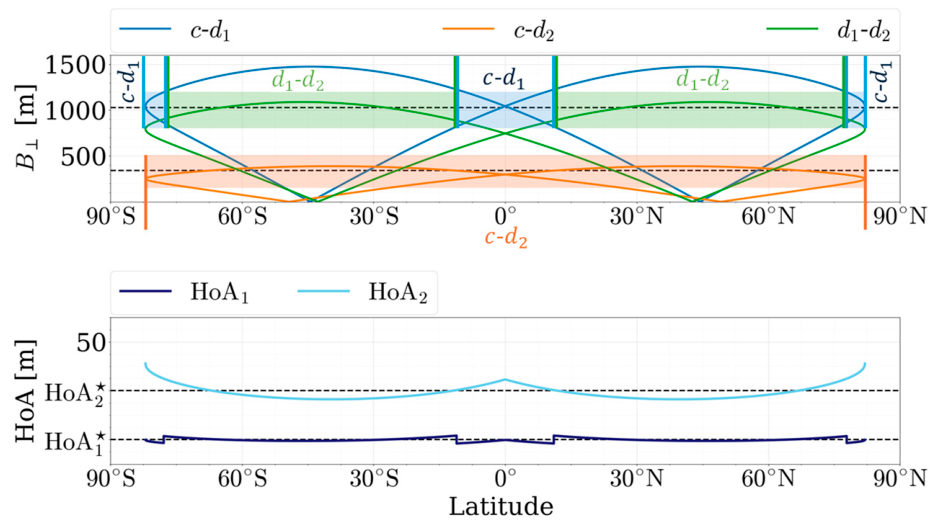
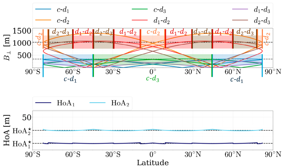
The heuristic solution is refined numerically with the genetic algorithms illustrated in Section 2.3.2. Figure 11 and Figure 12 display the effective baselines and selected HoAs obtained with the combination of SaDE and Compass algorithms with three and four satellites, respectively. Similarly to the heuristic case, these figures display the effective baseline in the top panel, with the colored bands indicating the chosen pair of satellites to produce the interferogram with the desired HoA. The bottom panels show instead the HoA coverage.

Four examples of optimal ROE sets that allow the obtained results in Figure 11 and Figure 12 are displayed in

Table 6. Example of ROEs for optimal three-satellite formation; safe configuration with same shape ratio.

ROE	Deputy 1	Deputy 2
$a_c\delta e$	1475 m	388 m
$\phi$	353.7°	348.8°
$a_c\delta i$	1475 m	388 m
$\vartheta$	173.7°	168.8°

,

Table 7. Example of ROEs for optimal four-satellite formation; safe configuration with same shape ratio.

ROE	Deputy 1	Deputy 2	Deputy 3
$a_c\delta e$	351 m	1394 m	352 m
$\phi$	11.3°	349.1°	326.4°
$a_c\delta i$	351 m	1394 m	352 m
$\vartheta$	11.3°	349.1°	326.4°

,

Table 8. Example of ROEs for optimal three-satellite formation; safe configuration with aligned vectors.

ROE	Deputy 1	Deputy 2
$a_c\delta e$	1875 m	449 m
$\phi$	90°	90°
$a_c\delta i$	1255 m	357 m
$\vartheta$	270°	270°

and

Table 9. Example of ROEs for optimal four-satellite formation; safe configuration with aligned vectors.

ROE	Deputy 1	Deputy 2	Deputy 3
$a_c\delta e$	584 m	1782 m	242 m
$\phi$	90°	90°	90°
$a_c\delta i$	161 m	1180 m	391 m
$\vartheta$	270°	270°	270°

. Specifically, Table 6 and Table 7 report the ROEs for passively safe formations where all the relative orbits have the same shape ratio (i.e., they are compliant with Equation (13)), for a three- and four-satellite formation, respectively. Table 8 and Table 9, instead, list the ROEs for scenarios where all the relative eccentricity and inclination vectors are collinear (i.e., passively safe according to Equation (12)), again for three- and four-satellite formations, respectively. The setup considered in this example involves acquiring images of the Northern Hemisphere in the ascending part of the orbit and vice versa for the Southern Hemisphere, achieving global coverage as in Figure 7. In these two quarters of the orbit, the error remains in the order of a meter or less, while the points where the satellites are located in an unfavorable geometry (which leads to vanishing effective baselines) are not used for imaging. Nevertheless, the reverse setup would have been equally viable. The RMSE has been computed employing the algorithms illustrated in Section 2.3.2 for formations of three and four satellites, respectively.

Table 10. RMSE achieved through SaDE + Compass Search, computed after 1000 generations of an initial population of 200 individuals.

${\mathbf{H}\mathbf{o}\mathbf{A}}_1$	${\mathbf{H}\mathbf{o}\mathbf{A}}_2$	3 Satellites		4 Satellites
		$\mathbf{R}\mathbf{M}\mathbf{S}\mathbf{E}\mathbf{H}\mathbf{o}{\mathbf{A}}_1$	$\mathbf{R}\mathbf{M}\mathbf{S}\mathbf{E}\mathbf{H}\mathbf{o}{\mathbf{A}}_2$	$\mathbf{R}\mathbf{M}\mathbf{S}\mathbf{E}\mathbf{H}\mathbf{o}{\mathbf{A}}_1$	$\mathbf{R}\mathbf{M}\mathbf{S}\mathbf{E}\mathbf{H}\mathbf{o}{\mathbf{A}}_2$
10 m	20 m	$4.9\%$	$10.5\%$	$3.8\%$	$2.0\%$
10 m	30 m	$7.0\%$	$10.4\%$	$3.5\%$	$2.3\%$
10 m	40 m	$5.4\%$	$10.4\%$	$3.6\%$	$2.4\%$
10 m	50 m	$4.9\%$	$10.4\%$	$3.0\%$	$2.4\%$

reports the result obtained by combining the SaDE and Compass Search algorithms, which yielded the lowest RMSE, for different ratios of the nominal HoAs.

The numerical results demonstrate that with a relatively small number of satellites—three are likely to be enough for most applications—it is possible to achieve two rather uniform HoAs for the mapping of the entire Earth’s surface. This, in turn, shows that multi-baseline formations can effectively overcome the limitation of the robustness/accuracy trade-off affecting single-baseline concepts. As expected, the numerical results are better than those obtained just with the heuristic. However, the relevance of the latter is not to be underestimated: it is derived directly from the analytical solution of the two-satellite case, and, therefore, it brings an understanding of how the ROE selection works that a purely numerical solution could not possibly provide. The RMSE reported in Table 10 can be linked to the DEM height error by means of the Cramér–Rao lower bound in Equation (1): at fixed $\gamma$ and $N_L$, the relative variation in the height uncertainty coincides with that of the HoA. Assuming $\gamma =0.8$ and $N_L=16$, one obtains ${\sigma }_h=0.21 \mathrm{m}$ for an HoA of 10 m; the 7% HoA variability therefore corresponds to a variation of about 1.5 cm, i.e., smaller than the variation caused by the spatial variability of the coherence within a typical scene.

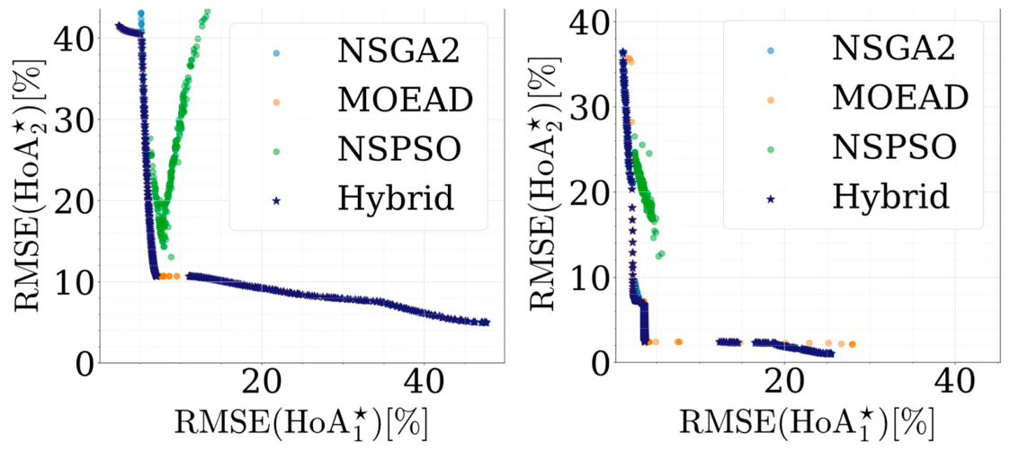
Finally, Figure 13 displays the Paretian solutions obtained with three different algorithms, namely Non-dominated Sorting Genetic Algorithm (NSGA2) [40], Multi-Objective Evolutionary Algorithm with Decomposition (MOEAD) [41], Non-dominated Sorting Particle Swarm Optimization (NSPSO) [42], and also those obtained by their hybridization. Note that the solution found by the single-objective optimization of Equation (19), solved through the combined use of the SaDE and Compass Search algorithms, is compliant with the solutions in the lower left part of the plots, confirming the robustness of such a solution also to different algorithms and random initialization seeds. A comparison between the algorithms reveals that the NSGA2 generates the most homogeneous distribution of Paretian solutions and has been proven to be effective even after a smaller number of generations. The MOEAD tends to find points more concentrated in clusters, especially after a short time, but it also identifies non-dominated solutions not recovered by the other two algorithms. Finally, the hybrid algorithm combines the advantages of the other three.

3.2.3. Effect of Earth’s Rotation

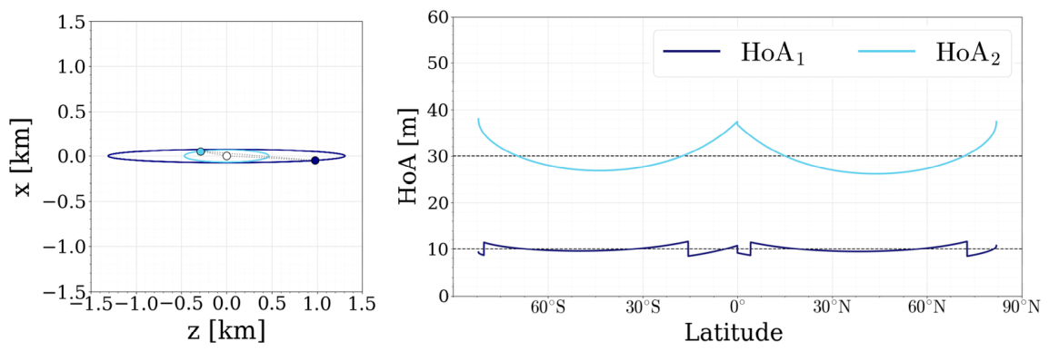
As anticipated in Section 2.1.2, the effect of Earth’s rotation on the inter-satellite distances causes the equations of motion to become coupled, making it inaccurate to consider the effective baseline as dependent solely on the x and z components of the Hill frame. Therefore, Equations (21) and (22), which allow to reformulate the effective baseline in terms of modulus and phase (both independent of $u$) in the Hill frame, are no longer applicable. Consequently, the optimization becomes more computationally demanding, as each ROE represents a separate decision variable (at least until more stringent requirements, such as passive-safety ones, are taken into account). Additionally, the HoA ceases to be $\pi$-periodic; its behavior is different in the two hemispheres due to the influence of Earth’s rotation, requiring the two integration intervals $u \in [0, \pi /2]$ and $u \in [\pi , 3\pi /2]$ to be considered separately. Since the analytical tools used previously are no longer viable, we proceed to calculate the optimal set of ROEs numerically, treating the along-track separation as an additional decision variable. This optimization is performed in the Earth-Centered–Earth-Fixed (ECEF) frame, in accordance with [30].

Table 11. Comparison between evaluated results taking into account Earth’s rotation.

Optimization	Minimum Distance [m]	$\mathbf{R}\mathbf{M}\mathbf{S}\mathbf{E}\left(\mathbf{H}\mathbf{o}{\mathbf{A}}_1\right)$	$\mathbf{R}\mathbf{M}\mathbf{S}\mathbf{E}\left(\mathbf{H}\mathbf{o}{\mathbf{A}}_2\right)$
in Hill frame	269	5.5$\%$	8.0$\%$
in ECEF	68	4.9$\%$	7.4$\%$

presents the optimal results for a three-satellite formation, assuming nominal HoA values of $10$ and $30$ m, respectively, and using the results for the non-rotating case as an initial guess. The solution found in this way is superior to the previous result due to the increased degrees of freedom: the Earth’s rotation is actively exploited to improve the performance. However, the minimum distance in the x–z plane between any pair of satellites decreases significantly compared to the cases examined in the previous formulation. The second row of Table 11 reports the results obtained from the optimized safe formation in the Hill frame, with performance re-evaluated to account for Earth’s rotation. It is observed that the discrepancy between the two solutions is negligible, suggesting that the initial formulation remains valid, particularly given its compliance with stricter safety constraints. The relative orbit and the HoA trend for the optimal case are shown in Figure 14. Specifically, the relative geometry in the left panel highlights reduced inter-satellite distances, resulting in a configuration with lower safety margins. Meanwhile, the right panel displays the selected HoAs: these closely resemble those of Figure 11, from which they differ because of the asymmetry of the smaller HoA curve around 0° latitude due to the differential impact of Earth’s rotation on the HoA across the two hemispheres.

It is worth remarking that the ECEF-optimized configuration is reported for verification purposes: its reduced minimum separation (less than 100 m) makes it operationally not feasible.

3.3. Optimal Generalized Helix Formations

This section is dedicated to the study of formations that are optimal and passively safe according to the requirements defined in Section 2.2 and Section 2.1.3, respectively. We therefore examine whether it is possible to design a generalized helix formation that is also interferometrically optimal in terms of coverage of the nominal HoA. Indeed, once the optimization is solved, the maximum effective baselines $B_{\perp \mathrm{m}\mathrm{a}\mathrm{x},j}$ and the corresponding angular shifts (${\delta }_1$ and ${\delta }_{1,j}$) defined in Equations (21) and (22) are fixed; the remaining task is to map these optimal baseline parameters back to a set of chief-referenced ROEs that is also compliant with mutual passive safety.

Under the helix orbit assumption, the ROEs of each deputy $j$ must satisfy the following relationships as a function of $B_{\perp \mathrm{m}\mathrm{a}\mathrm{x},j}$, ${\delta }_1$, and ${\delta }_{1,j}$:

$$\left\{\begin{array}{c}\delta i_j=\sqrt{{\displaystyle \frac{B_{\perp max,j}^2}{{\mathrm{c}\mathrm{o}\mathrm{s}}^2{\theta }_l}}-\delta e_j^2{\mathrm{t}\mathrm{a}\mathrm{n}}^2{\theta }_l}\\ {\phi }_1={\delta }_1\pm \arctan \left({\displaystyle \frac{\delta i_1}{\delta e_1\mathrm{t}\mathrm{a}\mathrm{n}{\theta }_l}}\right)\\ {\delta }_{1,j}-{\delta }_1+{\left(-1\right)}^n\arctan \left({\displaystyle \frac{\delta i_j}{\delta e_j\mathrm{t}\mathrm{a}\mathrm{n}{\theta }_l}}\right)\end{array}\right.$$

(37)

From the generalized-helix construction, mutual passive safety can be achieved under two alternative conditions: all chief-referenced relative orbits projected onto the $x-z$ plane are scaled versions of the same shape; or they share a common orientation of the relative eccentricity vectors (i.e., ${\phi }_i={\phi }_j+k\pi$ for all $i,j$). The compatibility of each option in Equation (37) is discussed below.

3.3.1. Safe Configuration with Orbits with Identical Shape Ratios

Without loss of generality, the first deputy is taken as the reference, and denoted with the subscript ${(·)}_1$. In the same shape ratio configuration, each other deputy ($j\ne 1$) must satisfy the shape-similarity condition:

$$\delta e_1 \delta i_j=\delta e_j \delta i_1.$$

(38)

Thus, substituting it into the first line of Equation (37) yields a simple proportionality between the eccentricity magnitudes and the optimized maximum effective baselines:

$$\begin{array}{c}\left({\displaystyle \frac{B_{\perp max,j}^2}{{\mathrm{c}\mathrm{o}\mathrm{s}}^2{\theta }_l}}-\delta e_j^2{\mathrm{t}\mathrm{a}\mathrm{n}}^2{\theta }_l\right)\delta e_1=\left({\displaystyle \frac{B_{\perp max,1}^2}{{\mathrm{c}\mathrm{o}\mathrm{s}}^2{\theta }_l}}-\delta e_1^2{\mathrm{t}\mathrm{a}\mathrm{n}}^2{\theta }_l\right)\delta e_j=0\\ \iff \delta e_j={\displaystyle \frac{B_{\perp max,j}}{B_{\perp max,1}}}\delta e_1.\end{array}$$

(39)

Consequently, all the magnitudes of the eccentricity vector must be in fixed ratios given by the maximum effective baselines with respect to that of the first deputy. The corresponding $\delta i_j$ is then recovered from the second line of Equation (37).

Regarding the phase of the relative eccentricity vector for the $j$-th deputy at optimality, by enforcing the respect of the last of Equation (37) the following requirement is obtained:

$${\phi }_j={\delta }_1-{\delta }_{1,j}+{\left(-1\right)}^n\mathrm{a}\mathrm{r}\mathrm{c}\mathrm{t}\mathrm{a}\mathrm{n}\sqrt{{\displaystyle \frac{B_{\perp \hspace{0.17em}\mathrm{m}\mathrm{a}\mathrm{x},1}^2}{\delta e_1^2{\mathrm{s}\mathrm{i}\mathrm{n}}^2{\theta }_l}}-1}.$$

(40)

Note that one decision variable ($\delta e_1$) remains undetermined: a practical implication is that the entire optimal-and-safe family can be tuned by selecting $\delta e_1$ so as to satisfy a minimum distance requirement. In particular, maximizing the minimum distance in the $x-z$ projection between any pair of satellites corresponds to the condition $\delta e=\delta i$, which yields circular relative orbits in the $x-z$ plane (xz-PCOs).

3.3.2. Safe Configuration with Common Orientation of the Eccentricity Vectors

The second passively safe option requires that all the phases of the deputies with respect to the chief are equal modulo $\pi$:

$${\phi }_i={\phi }_j+k\pi , \forall i,j; k\in \mathbb{Z}.$$

(41)

For compactness, we introduce the auxiliary variables:

$$\left\{\begin{array}{c}{E}_j:=\delta e_j\sin {\theta }_l\\ I_j:=\delta i_j\mathrm{c}\mathrm{o}\mathrm{s}{\theta }_l\end{array}\right..$$

(42)

Substituting the definition of ${\delta }_1$ into the last line of Equation (37) gives a direct constraint linking the optimized angular shifts ${\delta }_{1,j}$to the ratios $I_j/E_j$:

$${\delta }_{1,j}=k\pi +\mathrm{a}\mathrm{r}\mathrm{c}\mathrm{t}\mathrm{a}\mathrm{n}\left(\pm {\displaystyle \frac{I_j}{E_j}}\right)-\mathrm{a}\mathrm{r}\mathrm{c}\mathrm{t}\mathrm{a}\mathrm{n}\left(\pm {\displaystyle \frac{I_1}{E_1}}\right),\hspace{0.33em}k\in \mathbb{Z},$$

(43)

where the plus–minus signs in the arctangent functions depend on the relative orientation (parallel or anti-parallel) between the relative eccentricity and the relative inclination vectors. At this point, the condition given by the first equation of Equation (37) is imposed, obtaining:

$$\pm \mathrm{a}\mathrm{r}\mathrm{c}\mathrm{t}\mathrm{a}\mathrm{n}\left({\displaystyle \frac{\sqrt{B_{\perp max,j}^2-E_j^2}}{E_j}}\right)={\delta }_{1,j}+\mathrm{a}\mathrm{r}\mathrm{c}\mathrm{t}\mathrm{a}\mathrm{n}\left(\pm {\displaystyle \frac{I_1}{E_1}}\right)+k\pi$$

(44)

This constraint must be satisfied for every deputy $j$, again leaving one overall degree of freedom after enforcing all pairs. Since the arctangent is multi-valued, the admissible solutions depend on the sign choices and on the parity of $k$, and must satisfy the interval constraint that makes the inversion of Equation (44) valid. When admissible, Equation (44) can be inverted to obtain $E_j$ explicitly as:

$$E_j={\displaystyle \frac{B_{\perp max,j}}{\sqrt{1+{\mathrm{t}\mathrm{a}\mathrm{n}}^2\left({\delta }_{1,j}-k\pi +\mathrm{a}\mathrm{r}\mathrm{c}\mathrm{t}\mathrm{a}\mathrm{n}\left(\pm \frac{I_1}{E_1}\right)\right)}}}$$

(45)

For implementation, it is convenient to tabulate the admissible cases as a function of the quadrant of ${\delta }_{1,j}$, using the threshold values (introduced to delimit feasibility regions) $\delta e_T$ and $\delta e_C$ defined as follows:

$$\delta e_T:={\displaystyle \frac{B_{\perp max,1}}{\mathrm{s}\mathrm{i}\mathrm{n}{\theta }_l\sqrt{1+{\mathrm{t}\mathrm{a}\mathrm{n}}^2{\delta }_{1,j}}}},\delta e_C:={\displaystyle \frac{B_{\perp max,1}}{\mathrm{s}\mathrm{i}\mathrm{n}{\theta }_l\sqrt{1+{\mathrm{c}\mathrm{o}\mathrm{t}}^2{\delta }_{1,j}}}}$$

(46)

The results are listed in

Table 12. Conditions for safety and optimality.

(ϑ − φ)1	(ϑ − φ)j	φj − φ1	δ1j ∈ [0, π/2]	δ1j ∈ [π/2, π]	δ1j ∈ [π, 3π/2]	δ1j ∈ [3π/2, 2π]
0	0	0	$\delta e_1$ ≤ $\delta e_T$	—	—	$\delta e_1\ge \delta e_C$
0	0	π	—	$\delta e_1\ge \delta e_C$	$\delta e_1\le \delta e_T$	—
0	π	0	$\delta e_1\ge \delta e_T$	$\delta e_1\le \delta e_C$	--—	—
0	π	π	--	—	$\delta e_1\ge \delta e_T$	$\delta e_1\le \delta e_C$
π	0	0	—	—	$\delta e_1\le \delta e_C$	$\delta e_1\ge \delta e_T$
π	0	π	$\delta e_1\le \delta e_C$	$\delta e_1\ge \delta e_T$	—	—
π	π	0	$\delta e_1\ge \delta e_C$	—	—	$\delta e_1\le \delta e_T$
π	π	π	—	$\delta e_1\le \delta e_T$	$\delta e_1\ge \delta e_C$	—

. The solutions also depend on the quadrant to which the angle ${\delta }_{1,j}$ belongs; hence, once its value has been fixed by the optimization algorithm, only a portion of possible combinations of signs and parities of the $k$ parameter in Equation (44) allows for a passively safe configuration to be obtained.

Finally, besides the conditions imposed on the parameter $\delta e_1$ in Table 12, the ROEs of the $j$-th deputy relative to the chief must respect the following set of conditions:

$$\left\{\begin{array}{c}\delta e_j={\displaystyle \frac{\left(B_{\perp \hspace{0.17em}\mathrm{m}\mathrm{a}\mathrm{x},j}/\mathrm{s}\mathrm{i}\mathrm{n}{\theta }_l\right)}{\sqrt{1+{\mathrm{t}\mathrm{a}\mathrm{n}}^2\left({\delta }_{1,j}-{\mathrm{a}\mathrm{r}\mathrm{c}\mathrm{t}\mathrm{a}\mathrm{n}}^2\left(\frac{B_{\perp \hspace{0.17em}\mathrm{m}\mathrm{a}\mathrm{x},1}/{\mathrm{c}\mathrm{o}\mathrm{s}}^2{\theta }_l-\delta e_1^2{\mathrm{t}\mathrm{a}\mathrm{n}}^2{\theta }_l}{\delta e_1\mathrm{t}\mathrm{a}\mathrm{n}{\theta }_l}\right)\right)}}}\\ {\phi }_j={\delta }_1\pm \arctan \sqrt{{\displaystyle \frac{B_{\perp \hspace{0.17em}\mathrm{m}\mathrm{a}\mathrm{x},1}^2}{\delta e_1^2{\mathrm{s}\mathrm{i}\mathrm{n}}^2{\theta }_l}}-1}+k\pi \end{array}\right.$$

(47)

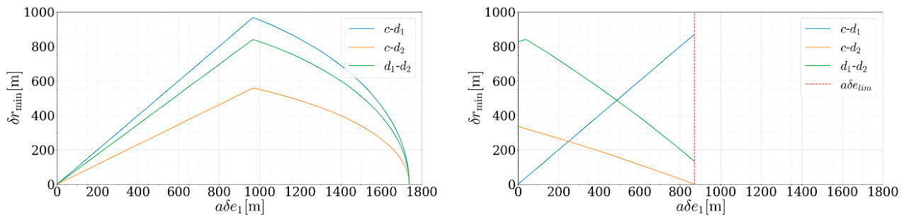
Equation (47) finally demonstrates that both the identified safe families (identical shape ratios and common orientation of the eccentricity vectors) are compatible with a set of optimal configurations, and remain defined up to one degree of freedom. This free parameter (taken in the following as $\delta e_1$) can be selected to enforce the minimum separation to be larger than a selected limit $\delta r_{\mathrm{m}\mathrm{i}\mathrm{n}}$. As an example, consider Figure 15, which displays the minimum distance in the x–z plane for each pair of satellites in an optimized formation of three. In particular, the left plot refers to the safe condition with parallel $∆\mathbf{e}$ and $∆\mathbf{i}$ vectors, while that on the right refers to scaled relative orbits. The value of $\delta e_1$ needed to maintain a certain minimum separation can be set so that none of the curves is, for that point, below the desired value. While the trend of the curves in the first case is determined by the conditions in Table 12, the second has an intuitive interpretation: the minimum distance is precisely given by $\delta e_1$ for the first deputy and proportional to it for other deputies, as long as $\delta e_1< \delta i_1$. In this region, the minimum distance is in fact obtained in a purely radial direction when the latitude argument $u = {\phi }_1$ is reached. Beyond the $\delta e_1= \delta i_1$ point, the minimum distance is obtained in the z-direction, when $u ={\phi }_1+\pi /2$ and depends on $\delta i_1$, which in turn is related to $\delta e_1$ through Equation (37). Finally, the minimum separation $\delta r_{min}$ goes back to zero when $\delta i_1= 0$ or $\delta e_1=B_{\perp max,1}/\mathrm{s}\mathrm{i}\mathrm{n}{\theta }_l$. A direct outcome is that the nested xz-PCO realization of the scaled-orbits family emerges as a notable configuration: it preserves HoA optimality while tending to maximize the minimum distance between any pair of satellites, making it an attractive operational design point when passive-safety margins dominate the design. It is worth remarking that, as also apparent in Figure 15, interferometric optimality and passive safety are decoupled: the optimal safe solution maintains one residual degree of freedom; thus, the required minimum separation can be enforced without worsening the HoA RMSE.

The aforementioned configurations in Table 6, Table 7, Table 8 and Table 9 are indeed examples of passively safe relative orbits that also generate optimal solutions. In particular, Table 6 and Table 7 correspond to a configuration where the relative orbits are such that $\delta e_i/\delta i_i=1$. Table 8 and Table 9, instead, lead to a formation where all pairs have the relative eccentricity and inclination vectors lying in the same direction for the case ${\phi }_i={\vartheta }_i=\pi /2+k\pi$: this solution has the advantage of requiring less control effort to counterbalance the secular effects of the $J_2$ perturbation.

3.4. Formation Maintenance

In this section we provide the estimate of the formation-keeping costs employing the strategies outlined in Section 2.4 and applying them to the optimal and passively safe configurations identified in Section 3.3 for both the categories of generalized helix: the one with equal orbit shape ratio, and the one with a common orientation of the eccentricity vectors.

The numerical results are listed in

Table 13. Three-satellite formation maintenance cost, optimal configuration in a dawn–dusk SSO, ${\mathcal{S}}_2$ with along-track maneuver after 100 m.

$\overline{\mathsf{\rho }}$ [kg/m3]	ΔCB [m2/kg]	Absolute Drag Compensation [m/s/T]	$\mathbf{\Delta }\mathbf{v}{\mathcal{S}}_1$ [m/s/T]	$\mathbf{\Delta }\mathbf{v}{\mathcal{S}}_2$ [m/s/T]	$\mathbf{\Delta }\mathbf{v}$ for $\mathit{\vartheta }=\mathit{\pi }/2$ [m/s/T]
1 × 10−12	0	0.033	0.017	0.017	0.0004
1 × 10−12	5 × 10−3	0.033	0.019	0.019	0.0018
1 × 10−12	1 × 10−2	0.033	0.021	0.021	0.0033
3 × 10−12	5 × 10−3	0.054	0.022	0.022	0.0051
3 × 10−12	1 × 10−2	0.054	0.028	0.027	0.0099
5 × 10−12	5 × 10−3	0.081	0.026	0.026	0.0083
5 × 10−12	1 × 10−2	0.081	0.034	0.044	0.0168

and

Table 14. Four-satellite formation maintenance cost, optimal configuration in a dawn–dusk SSO, ${\mathcal{S}}_2$ with along-track maneuver after 100 m.

$\overline{\mathsf{\rho }}$ [kg/m3]	ΔCB [m2/kg]	Absolute Drag Compensation [m/s/T]	$\mathbf{\Delta }\mathbf{v}$ S1 [m/s/T]	$\mathbf{\Delta }\mathbf{v}$ S2 [m/s/T]	$\mathbf{\Delta }\mathbf{v}$ for $\mathit{\vartheta }=\mathit{\pi }/2$ [m/s/T]
1 × 10−12	0	0.044	0.024	0.024	0.0009
1 × 10−12	5 × 10−3	0.044	0.027	0.027	0.0018
1 × 10−12	1 × 10−2	0.044	0.029	0.029	0.0037
3 × 10−12	5 × 10−3	0.072	0.032	0.032	0.0060
3 × 10−12	1 × 10−2	0.072	0.039	0.039	0.0149
5 × 10−12	5 × 10−3	0.108	0.037	0.037	0.0208
5 × 10−12	1 × 10−2	0.108	0.049	0.049	0.0248

, reporting the formation maintenance cost ($\Delta \mathrm{v}$) per orbital period (T) for the interferometrically optimal configurations for three and four satellites respectively, considering the two types of notable generalized helix configurations (with scaled relative orbits and aligned $\Delta \mathbf{e}, \Delta \mathbf{i}$ vectors). The first column reports the average air density: since its dependence on the altitude is highly influenced by solar and geomagnetic activities, we consider three exemplary values of $1, 3, \mathrm{a}\mathrm{n}\mathrm{d} 5\times {10}^{-12}{\displaystyle \frac{\mathrm{k}\mathrm{g}}{{\mathrm{m}}^3}},$ to represent quiet, moderate and intense solar and geomagnetic activities, respectively, for the altitude range considered in Table 1. The third column reports the $∆\mathrm{v}$ per orbital period required to compensate for the semi-major axis decay caused by absolute drag.

The last three columns show the results for three different configurations:

• Helix formation considering a control strategy based on ${\mathcal{S}}_1$ (coupled $\delta a-\delta l$ management, see Section 2.4).
• Helix formation considering a control strategy based on ${\mathcal{S}}_2$ (threshold-triggered along-track maneuver, see Section 2.4).
• Helix formation with $\vartheta = \pi /2$ considering a control strategy based on ${\mathcal{S}}_1$. In this last case, the strategy ${\mathcal{S}}_2$ is not reported since the numerical results are practically indistinguishable.

The results show that the required control effort increases at lower altitudes and when there are greater differences in ballistic coefficients. More interestingly, the configuration with $\vartheta =\pi /2$yields the minimum cost among the considered safe families because it suppresses the secular $J_2$-driven drift in the relative inclination vector. Therefore, this eliminates the need for out-of-plane corrections. However, the advantage of adopting a common orientation of the eccentricity vectors diminishes as the contribution of air drag becomes more significant relative to that of $J_2$, ranging from requiring a $∆\mathrm{v}$ of $\approx 2\%$ compared to the configuration with orbits of identical shape ratios in the absence of differential air drag, to $\approx 50\%$ in the case of lower altitude/higher solar activity and maximum difference between ballistic coefficients. Therefore, the required control effort becomes almost negligible, especially when compared with that necessary to counteract the semi-major axis decay caused by absolute drag.

3.5. Design Synthesis and Exemplary Configurations

This section presents a comprehensive overview of the introduced methodology for the identification of suitable formation flying solutions and some exemplary configurations following the proposed design.

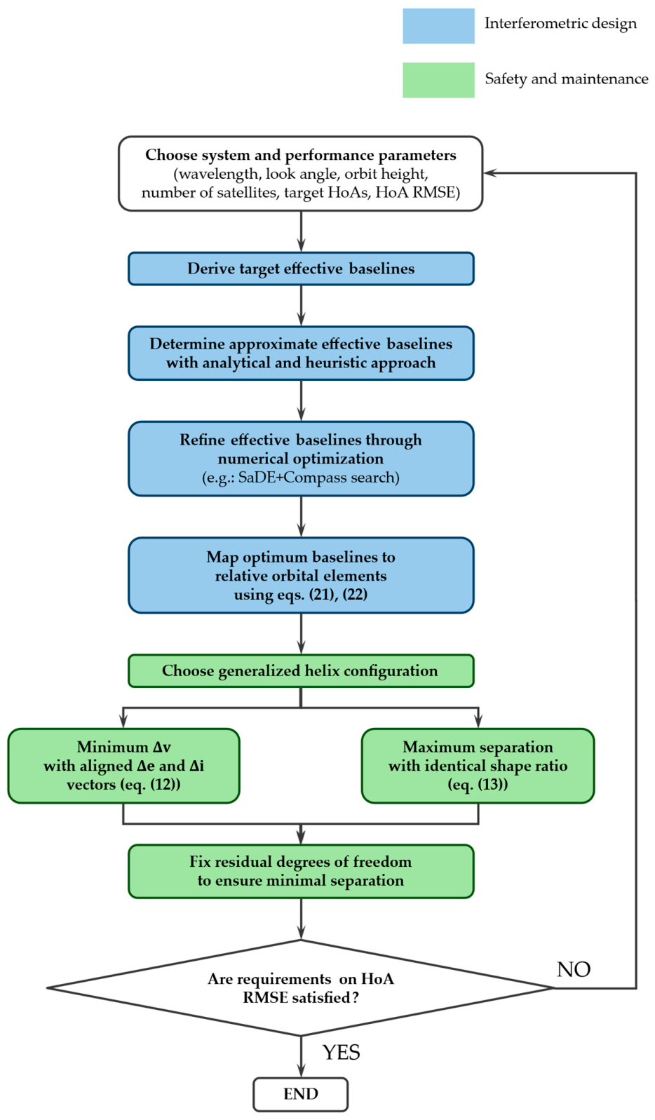
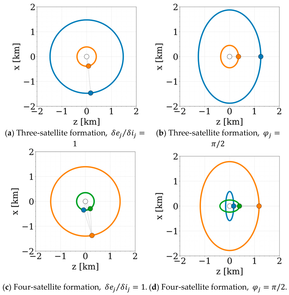
Specifically, Figure 16 reports the key design steps to be followed in a hypothetical mission design case, as illustrated through this study. Note that, depending on the specific mission requirements, the system parameters may be set either entirely or partially. Four exemplary design solutions are then listed in

Table 15. Exemplary configurations with three/four satellites, interferometric and safety performance, assuming: $\overline{\rho }=3\cdot {10}^{-12} \mathrm{k}\mathrm{g}/{\mathrm{m}}^3$, pessimistic ballistic coefficient difference $\Delta C_B=0.01 {\mathrm{m}}^2/\mathrm{k}\mathrm{g}$, X-band, angle of incidence $={37}^{\circ }$, and dawn–dusk SSO.

No. of Satellites	Configuration	Target HoAs	Max Effective Baseline	Min Distance x-z Plane	HoA RMSE	$\mathbf{\Delta }\mathbf{v} \mathbf{p}\mathbf{e}\mathbf{r}$ Orbit	$\mathbf{\Delta }\mathbf{v} \mathbf{p}\mathbf{e}\mathbf{r}$ Year
3	same shape ratio	10 m 30 m	1475.12 m	416.62 m	7.0% 10.4%	0.028 m/s	115.33 m/s
3	aligned vectors	10 m 30 m	1475.12 m	357.52 m	7.0% 10.4%	0.010 m/s	40.78 m/s
4	same shape ratio	10 m 30 m	1394.88 m	269.43 m	3.5% 2.3%	0.039 m/s	160.64 m/s
4	aligned vectors	10 m 30 m	1394.88 m	161.59 m	3.5% 2.3%	0.015 m/s	61.37 m/s

: these are the two notable configurations identified (with identical shape ratio and aligned relative eccentricity and inclination vectors) for formations of three and four satellites and exemplary target HoAs of 10 and 30 m, assuming a dawn–dusk SSO at an altitude of 500 km, an average air density of $\overline{\rho }=3\cdot {10}^{-12}{\displaystyle \frac{\mathrm{k}\mathrm{g}}{{\mathrm{m}}^3}}$ corresponding to moderate solar and geomagnetic activities, a ballistic coefficient difference $\Delta C_B=0.01 {\mathrm{m}}^2/\mathrm{k}\mathrm{g}$, and an angle of incidence of ${37}^{\circ }$. Note how, in a comparison between formations with the same number of satellites, there is a trade-off between the minimum inter-satellite distance and the $\Delta \mathrm{v}$ required for the formation keeping, with the solutions with same shape ratio and aligned $\Delta \mathbf{e}$ and $\Delta \mathbf{i}$ vectors achieving the safest and cheapest configurations, respectively. Moreover, the addition of a fourth satellite leads to an improvement in terms of HoA RMSE at the cost of a higher $\Delta \mathrm{v}$ and reduced minimum inter-satellite separation. The four proposed formations are then displayed in the four panels of Figure 17, for which the ROEs correspond to those already identified in the optimization process in Table 6, Table 7, Table 8 and Table 9.

4. Discussion

This study addresses the design of optimal satellite formations for single-pass, multi-baseline spaceborne SAR interferometry for the generation of high-quality DEMs. The underlying idea is to deliver interferograms with two distinct HoAs that guarantee both height accuracy and robustness to phase unwrapping errors through the use of formations that are safe and require minimal control effort.

The results demonstrate that it is indeed possible to obtain two rather uniform HoAs with only three satellites. The variability of the two HoAs obtained, which is in the order of 10% for the three-satellite case, is perfectly acceptable for interferometry applications. This is because performance consistency is influenced by coherence, which, in any case, varies spatially: typically, the ratio between the HoAs is required to fall within a fairly wide range, from 2.5 to 4, in order to correct phase unwrapping errors [20,21,23]. A possible application scenario for the three-satellite configuration is the concept based on one CubeSat add-on to a TanDEM-X-like interferometer proposed in [23], where the formation could be designed to achieve the lowest HoA using the same pair at all latitudes. Moreover, if the possibility of adding a fourth satellite is allowed, the variability of the achieved HoAs lowers to about 3%. Nevertheless, this would result in only a marginal improvement in the DEM performance and might not justify the additional cost.

As an intermediate step of the analysis, we have studied the two-satellite case (single-baseline, single-pass SAR interferometry), for which an analytical solution has been derived that establishes a closed-form relationship between the ROEs, the effective baseline, and the HoA as a function of the latitude. This has immediate application (in combination with previous results regarding the optimization of the incidence angle in [28]) to the design and operation of bistatic missions like TanDEM-X.

It is shown that nested helix formations can meet interferometric and passive-safety requirements simultaneously, with two particularly noteworthy configurations. In the first one, all relative orbits have the same shape: this allows for the minimum distance to be maximized between each pair of satellites, ensuring maximum safety. Such a solution could therefore be suitable for maintaining maximum HoA consistency when short baselines are employed, which is particularly relevant for high-frequency applications. A second solution, a direct generalization of the single-baseline case implemented in TanDEM-X, ensures stability against orbital perturbations caused by the oblateness term of the geopotential. Thus, it minimizes the formation maintenance cost. The study of formation maintenance cost shows that the optimal configurations can be maintained with minimal fuel expenses: in the examined scenarios the Δv budget required for formation keeping is indeed well below the amount required to counteract the semi-major axis’ decay caused by aerodynamic drag affecting the entire formation.

The results presented in this paper provide an important step forward for the design of future multi-baseline SAR interferometry missions aimed at DEM generation with a single-pass acquisition strategy. Promising extensions could include a more accurate model of dynamics, incorporating additional geopotential terms beyond J₂ and other perturbations not limited to a basic model of atmospheric drag. The identified optimal formations should be supported by efficient guidance, navigation and control algorithms: the development of suitable strategies, tailored to such specific configurations, is therefore a natural next step. Finally, the optimization framework could be expanded so as to consider metrics other than the HoA coverage, such as coherence, region-specific coverage, and wavelength/bandwidth trade-offs. Concerning the coherence, it might be increased by leveraging the SNR through the novel SwitchSAR mode [43], or traded off with the data rate through quantization with variable bit rate [44,45]. In a more holistic perspective, new strategies could be investigated, such as the adoption of a mixed approach involving fixed and time-varying baselines, and envisioning an extension to SAR tomography and other multi-static and distributed SAR applications.

References

1. Moreira, A.; Prats-Iraola, P.; Younis, M.; Krieger, G.; Hajnsek, I.; Papathanassiou, K.P. A Tutorial on Synthetic Aperture Radar. IEEE Geosci. Remote Sens. Mag. 2013, 1, 6–43. [Google Scholar] [CrossRef] [Scilit]
2. Bamler, R.; Hartl, P. Synthetic Aperture Radar Interferometry. Inverse Probl. 1998, 14, R1. [Google Scholar] [CrossRef] [Scilit]
3. Rosen, P.A.; Hensley, S.; Joughin, I.R.; Li, F.K.; Madsen, S.N.; Rodriguez, E.; Goldstein, R.M. Synthetic Aperture Radar Interferometry. Proc. IEEE 2000, 88, 333–382. [Google Scholar] [CrossRef] [Scilit]
4. Hanssen, R.F. Radar Interferometry: Data Interpretation and Error Analysis; Remote Sensing and Digital Image Processing; Springer: Dordrecht, The Netherlands, 2001; Volume 2. [Google Scholar]
5. Ferretti, A.; Prati, C.; Rocca, F. Permanent Scatterers in SAR Interferometry. IEEE Trans. Geosci. Remote Sens. 2001, 39, 8–20. [Google Scholar] [CrossRef] [Scilit]
6. Berardino, P.; Fornaro, G.; Lanari, R.; Sansosti, E. A New Algorithm for Surface Deformation Monitoring Based on Small Baseline Differential SAR Interferograms. IEEE Trans. Geosci. Remote Sens. 2002, 40, 2375–2383. [Google Scholar] [CrossRef] [Scilit]
7. Ferretti, A.; Fumagalli, A.; Novali, F.; Prati, C.; Rocca, F.; Rucci, A. A New Algorithm for Processing Interferometric Data-Stacks: SqueeSAR. IEEE Trans. Geosci. Remote Sens. 2011, 49, 3460–3470. [Google Scholar] [CrossRef] [Scilit]
8. Krieger, G.; Moreira, A. Spaceborne Bi- and Multistatic SAR: Potential and Challenges. IEE Proc.—Radar Sonar Navig. 2006, 153, 184–198. [Google Scholar] [CrossRef] [Scilit]
9. Moreira, A.; Krieger, G.; Villano, M.; Younis, M.; Prats-Iraola, P.; Zink, M. Spaceborne Synthetic Aperture Radar: Future Technologies and Mission Concepts. Proc. IEEE 2025, 114, 183–219. [Google Scholar] [CrossRef] [Scilit]
10. Hu, C.; Li, Y.; Chen, Z.; Liu, F.; Zhang, Q.; Monti-Guarnieri, A.V.; Hobbs, S.; Anghel, A.; Datcu, M. Distributed Spaceborne SAR: A Review of Systems, Applications, and the Road Ahead. IEEE Geosci. Remote Sens. Mag. 2025, 13, 329–361. [Google Scholar] [CrossRef] [Scilit]
11. Krieger, G.; Moreira, A.; Fiedler, H.; Hajnsek, I.; Werner, M.; Younis, M.; Zink, M. TanDEM-X: A Satellite Formation for High-Resolution SAR Interferometry. IEEE Trans. Geosci. Remote Sens. 2007, 45, 3317–3341. [Google Scholar] [CrossRef] [Scilit]
12. Hajnsek, I.; Busche, T.; Abdullahi, S.; Bachmann, M.; Baumgartner, S.V.; Bojarski, A.; Bueso-Bello, J.-L.; Esch, T.; Fritz, T.; Alonso-Gonzalez, A.; et al. TanDEM-X: The 4D Mission Phase for Earth Surface Dynamics: Science Activities Highlights and New Data Products after 15 Years of Bistatic Operations. IEEE Geosci. Remote Sens. Mag. 2025, 13, 116–151. [Google Scholar] [CrossRef] [Scilit]
13. D’Amico, S.; Montenbruck, O. Proximity Operations of Formation-Flying Spacecraft Using an Eccentricity/Inclination Vector Separation. J. Guid. Control Dyn. 2012, 29, 554–563. [Google Scholar] [CrossRef] [Scilit]
14. Koenig, A.W.; D’Amico, S. Robust and Safe N-Spacecraft Swarming in Perturbed Near-Circular Orbits. J. Guid. Control Dyn. 2018, 41, 1643–1662. [Google Scholar] [CrossRef] [Scilit]
15. Scala, F.; Peixoto, M.N.; Krieger, G.; Villano, M. On the Safety of Multiple Satellite Formations for Synthetic Aperture Radar Applications. J. Guid. Control Dyn. 2025, 48, 414–423. [Google Scholar] [CrossRef] [Scilit]
16. Lopez-Dekker, P.; Stoffelen, A.; Kääb, A.; Hooper, A.; Rabus, B.; Chapron, B.; Buongiorno Nardelli, B.; Muller, C.; Pasquero, C.; Muller, J.-P.; et al. Harmony: Science Objectives and Mission Overview. In Proceedings of the ESA Living Planet Symposium 2022, Bonn, Germany, 23–27 May 2022. [Google Scholar]
17. Cotugno, F.; Theodosiou, A.; Rommen, B.; Manunta, M.; Lanari, R.; Salvato, M.; Pelliccia, F.; Renga, A. Optimization of Formation Parameters for Single-Pass/Cross-Track Interferometry Through the Harmony Mission. Remote Sens. 2026, 18, 877. [Google Scholar] [CrossRef] [Scilit]
18. Deng, Y.; Zhang, H.; Liu, K.; Wang, W.; Ou, N.; Han, H.; Yang, R.; Ren, J.; Wang, J.; Ren, X.; et al. Hongtu-1: The First Spaceborne Single-Pass Multibaseline SAR Interferometry Mission. IEEE Trans. Geosci. Remote Sens. 2025, 63, 5202518. [Google Scholar] [CrossRef] [Scilit]
19. Massonnet, D. Capabilities and Limitations of the Interferometric Cartwheel. IEEE Trans. Geosci. Remote Sens. 2001, 39, 506–520. [Google Scholar] [CrossRef] [Scilit]
20. Lachaise, M.; Fritz, T.; Balss, U.; Bamler, R.; Eineder, M. Phase Unwrapping Correction with Dual-Baseline Data for the TanDEM-X Mission. In 2012 IEEE International Geoscience and Remote Sensing Symposium; IEEE: Piscataway, NJ, USA, 2012; pp. 5566–5569. [Google Scholar]
21. Lachaise, M.; Fritz, T.; Bamler, R. The Dual-Baseline Phase Unwrapping Correction Framework for the TanDEM-X Mission Part 1: Theoretical Description and Algorithms. IEEE Trans. Geosci. Remote Sens. 2018, 56, 780–798. [Google Scholar] [CrossRef] [Scilit]
22. Eineder, M.; Adam, N. A Maximum-Likelihood Estimator to Simultaneously Unwrap, Geocode, and Fuse SAR Interferograms from Different Viewing Geometries into One Digital Elevation Model. IEEE Trans. Geosci. Remote Sens. 2005, 43, 24–36. [Google Scholar] [CrossRef] [Scilit]
23. Nogueira Peixoto, M.; Krieger, G.; Moreira, A.; Waldschmidt, C.; Villano, M. On the Exploitation of CubeSats for Highly Accurate and Robust Single-Pass SAR Interferometry. IEEE Trans. Geosci. Remote Sens. 2023, 61, 5217216. [Google Scholar] [CrossRef] [Scilit]
24. Scala, F.; Villano, M. Optimal Orbit Altitude of Satellite Formations for Across-Track SAR Interferometry. IEEE Trans. Geosci. Remote Sens. 2026, 64, 5201619. [Google Scholar] [CrossRef] [Scilit]
25. D’Amico, S. Autonomous Formation Flying in Low Earth Orbit. Ph.D. Thesis, Technische Universiteit Delft, Delft, The Netherlands, 2010. [Google Scholar]
26. Clohessy, W.H.; Wiltshire, R.S. Terminal Guidance System for Satellite Rendezvous. J. Aerosp. Sci. 1960, 27, 653–658. [Google Scholar] [CrossRef] [Scilit]
27. D’Errico, M. (Ed.) Distributed Space Missions for Earth System Monitoring; Springer: New York, NY, USA, 2013. [Google Scholar]
28. Longari, R.; Scala, F.; Gaias, G.; Krieger, G.; Villano, M. Incidence Angle Optimization for Formation-Flying Across-Track SAR Interferometry. IEEE Geosci. Remote Sens. Lett. 2026, 23, 4004005. [Google Scholar] [CrossRef] [Scilit]
29. Fiedler, H.; Boerner, E.; Mittermayer, J.; Krieger, G. Total Zero Doppler Steering—A New Method for Minimizing the Doppler Centroid. IEEE Geosci. Remote Sens. Lett. 2005, 2, 141–145. [Google Scholar] [CrossRef] [Scilit]
30. Rodrigues-Silva, E.; Matar, J.; Rodriguez-Cassola, M.; Sakar, N.; Katz, R.; Kahle, R.; Moreira, A. Relative Orbit Design and Optimization for Distributed SAR Formations. IEEE Trans. Geosci. Remote Sens. 2025, 63, 5222514. [Google Scholar] [CrossRef] [Scilit]
31. Polak, E. Optimization: Algorithms and Consistent Approximations; Springer: Berlin/Heidelberg, Germany, 2012. [Google Scholar]
32. Hansen, N.; Ostermeier, A. Completely Derandomized Self-Adaptation in Evolution Strategies. Evol. Comput. 2001, 9, 159–195. [Google Scholar] [CrossRef] [Scilit] [PubMed]
33. Qin, A.K.; Huang, V.L.; Suganthan, P.N. Differential Evolution Algorithm with Strategy Adaptation for Global Numerical Optimization. IEEE Trans. Evol. Comput. 2009, 13, 398–417. [Google Scholar] [CrossRef] [Scilit]
34. Karaboga, D.; Basturk, B. A Powerful and Efficient Algorithm for Numerical Function Optimization: Artificial Bee Colony (ABC) Algorithm. J. Glob. Optim. 2007, 39, 459–471. [Google Scholar] [CrossRef] [Scilit]
35. Kolda, T.G.; Lewis, R.M.; Torczon, V. Optimization by Direct Search: New Perspectives on Some Classical and Modern Methods. SIAM Rev. 2003, 45, 385–482. [Google Scholar] [CrossRef] [Scilit]
36. Vallado, D.A. Fundamentals of Astrodynamics and Applications; Springer: Berlin/Heidelberg, Germany, 2001. [Google Scholar]
37. Picone, J.M.; Hedin, A.E.; Drob, D.P.; Aikin, A.C. NRLMSISE-00 Empirical Model of the Atmosphere: Statistical Comparisons and Scientific Issues. J. Geophys. Res. 2002, 107, 1468. [Google Scholar] [CrossRef] [Scilit]
38. Willis, M.; D’Amico, S. Analytical Description of Relative Position and Velocity on J2-Perturbed Eccentric Orbits. In Proceedings of the 31st AAS/AIAA Space Flight Mechanics Meeting, Virtual, 31 January–4 February 2021. [Google Scholar]
39. Gaias, G.; D’Amico, S. Impulsive Maneuvers for Formation Reconfiguration Using Relative Orbital Elements. J. Guid. Control Dyn. 2015, 38, 1036–1049. [Google Scholar] [CrossRef] [Scilit]
40. Deb, K.; Pratap, A.; Agarwal, S.; Meyarivan, T. A Fast and Elitist Multiobjective Genetic Algorithm: NSGA-II. IEEE Trans. Evol. Comput. 2002, 6, 182–197. [Google Scholar] [CrossRef] [Scilit]
41. Zhang, Q.; Li, H. MOEA/D: A Multiobjective Evolutionary Algorithm Based on Decomposition. IEEE Trans. Evol. Comput. 2007, 11, 712–731. [Google Scholar] [CrossRef] [Scilit]
42. Liu, Y. A Fast and Elitist Multi-Objective Particle Swarm Algorithm: NSPSO. In 2008 IEEE International Conference on Granular Computing; IEEE: Piscataway, NJ, USA, 2008; pp. 470–475. [Google Scholar]
43. Villano, M. SwitchSAR: A Novel SAR Mode for Low NESZ Stripmap Imaging. In Proceedings of the European Conference on Synthetic Aperture Radar, EUSAR, Baden-Baden, Germany, 8–11 June 2026. [Google Scholar]
44. Martone, M.; Gollin, N.; Rizzoli, P.; Krieger, G. Performance-Optimized Quantization for SAR and InSAR Applications. IEEE Trans. Geosci. Remote Sens. 2022, 60, 5229922. [Google Scholar] [CrossRef] [Scilit]
45. Gollin, N.; Martone, M.; Imbembo, E.; Ghiglione, M.; Knoll, S.; Krieger, G.; Rizzoli, P. AI-BAQ: Deep Learning for Adaptive SAR Raw Data Quantization. IEEE Trans. Geosci. Remote Sens. 2025, 63, 5220620. [Google Scholar] [CrossRef] [Scilit]
Figure 1. Magnitude and phase of the relative vectors. Left: relative eccentricity vector. Right: relative inclination vectors. The chief’s parameters are denoted with the subscript ( · ) 1 and the deputy’s with ( · ) 2 . The relative vector representation follows the formulation presented in [13].
Remotesensing 18 03041 g001
Figure 2. Acquisition geometry in the x–z plane of the Hill frame.
Remotesensing 18 03041 g002
Figure 3. Example of effective baseline and HoA with respect to the latitude.
Remotesensing 18 03041 g003
Figure 4. Examples of geometries of the relative e/i vectors for maximum safety configuration for a four-satellite formation (one chief and three deputies di), leading to six relative e/i vectors. Left: equal phase differences. Right: same shape-relative orbits.
Remotesensing 18 03041 g004
Figure 5. Left, Center: optimal configuration compatible with passive safety. Right: incompatible configuration.
Remotesensing 18 03041 g005
Figure 6. x–z projection of relative orbits between each pair of a four-satellite generalized helix formation. Left: Common orientation of the eccentricity vectors; right: equal orbit shape ratio. Satellites’ relative positions are reported at the equator and denoted by dots.
Remotesensing 18 03041 g006
Figure 7. Latitudes considered in the optimization problem for a circular polar orbit. The blue arrow indicates the set U considered in the optimization problem, whereas the green area denotes the portion of Earth surface over which the formation will maintain the identified optimal configuration.
Remotesensing 18 03041 g007
Figure 8. Normalized L 2 -norm error for   H o A = 20 m with color scale saturated above 95th percentile; analytical curve traced in magenta.
Remotesensing 18 03041 g008
Figure 9. Effective baseline and HoA from the heuristic solution for a three-satellite formation. Top: effective baselines achieved at each latitude; the colored bands correspond to the satellite pair selected at a specific latitude. Bottom: HoAs of the two interferograms produced from the selected effective baselines. c indicates the chief, d i the i -th deputy. The dashed lines indicate the target HoAs (marked as H o A 1 and H o A 2 ) and the corresponding effective baselines.
Remotesensing 18 03041 g009
Figure 10. Effective baseline and HoA from the heuristic solution for a four-satellite formation. The dashed lines indicate the target HoAs (marked as H o A 1 and H o A 2 ) and the corresponding effective baselines.
Remotesensing 18 03041 g010
Figure 11. Optimal solution for a three-satellite formation: SaDE + Compass Search. (Top): effective baselines achieved at each latitude; the colored bands correspond to the satellite pair selected at a specific latitude. Bottom: HoAs of the two interferograms produced from the selected effective baselines. c indicates the chief, d i the i -th deputy. The dashed lines indicate the target HoAs (marked as H o A 1 and H o A 2 ) and the corresponding effective baselines.
Remotesensing 18 03041 g011
Figure 12. Optimal solution for a four-satellite formation: SaDE + Compass Search. The dashed lines indicate the target HoAs (marked as H o A 1 and H o A 2 ) and the corresponding effective baselines.
Remotesensing 18 03041 g012
Figure 13. Paretian solutions for different algorithms. Left: three-satellite formation. Right: four-satellite formation. The root mean square errors are reported in percentage of the target HoAs, marked as H o A 1 and H o A 2 .
Remotesensing 18 03041 g013
Figure 14. Numerically optimized formation on the x–z plane of the Hill frame and HoA, both resulting from the optimization in the ECEF frame to account for Earth’s rotation. The dashed lines indicate the target HoAs.
Remotesensing 18 03041 g014
Figure 15. Minimum distances between all satellite pairs as a function of the magnitude of one relative eccentricity vector for a three-satellite formation with optimum maximum effective baselines: B m a x , 1 = 967   m ,   B m a x , 2 = 558   m ,     B m a x , 3 = 1367   m .
Remotesensing 18 03041 g015
Figure 16. Design flow for single-pass multi-baseline interferometric formation. Blue: interferometric geometry steps. Green: passive-safety margin and formation-keeping steps, independent of achieved HoAs.
Remotesensing 18 03041 g016
Figure 17. Exemplary optimal and passively safe configurations for target HoAs   =   10   m , 30   m , projected onto the x–z plane of the Hill frame; satellites’ relative positions are reported at the equator and denoted by dots.
Remotesensing 18 03041 g017