Co-Burn: Combining dNBR Anchoring and Ordinal Learning for Cross-Event Fire Severity Mapping in New South Wales

Highlights

What are the main findings?

• Co-Burn attaches the pre-to-post dNBR to the post-fire branch as a change anchor and uses a conditional ordinal head to sequence burned-footprint placement before high-severity assignment.
• Across 14 New South Wales fires with four complete external holdouts, Co-Burn ranked first among ten methods under both pixel-pooled and event-mean aggregation, giving the strongest performance on fires excluded from training, validation, and model selection.

What are the implications of the main findings?

• For post-fire mapping of previously unseen forest wildfires, Co-Burn enables ordered three-class severity mapping without target-fire threshold calibration, using dNBR as a learned change anchor.
• Co-Burn delivers a more selective burned-footprint map, reducing false-burn expansion relative to the reflectance-only conditional variant, while reaching higher burned mIoU at the same false-burn budget.

Abstract

Cross-event fire-severity mapping requires a model to delineate the burned footprint and grade severity within it across wildfires whose spectral expression varies with vegetation and observation conditions. Nominal multiclass models treat the classes as parallel alternatives and leave the order implicit. We introduce Co-Burn, a bi-temporal Siamese model that adds a pre-to-post dNBR channel to the post-fire branch as an NIR-SWIR change anchor and uses a conditional ordinal head to estimate burn presence before high-severity assignment. Ten methods were compared across 14 New South Wales wildfires against a Sentinel-2 FESM-derived three-class target, with 4 complete fires held out from model development and selection. Co-Burn ranked first under both pixel-pooled and event-mean aggregation, reaching 0.520 ± 0.017 and 0.524 ± 0.028 external burned mIoU. Event-level factorial contrasts showed that burned-mIoU effects varied among fires, while dNBR anchoring reduced false-burn rate on all four external events. At the fixed operating point, Co-Burn assigned 19.9% of reference-unburned pixels to burned classes, against 28.9% for the reflectance-only nominal variant. On the hardest held-out fire, limited false-burn expansion coexisted with a downward shift across the ordered severity classes. Co-Burn supports ordered three-class mapping of previously unseen forest fires before target-fire labels become available.

1. Introduction

Post-fire burn-severity mapping centres on two interrelated questions across fire events: where are the fire-affected areas, and how severe are the impacts within them? The frequency and intensity of extreme wildfires have increased more than twofold globally over the past two decades, with the largest gains in temperate and boreal conifer biomes [1]. Reliable and consistent burn-severity maps can guide post-fire recovery, carbon accounting, and ecosystem assessment [2,3]. The 2019–2020 Australian Black Summer fires burned an unprecedented area of temperate forest [4] and exposed how difficult it is to assess severity consistently over such extensive landscapes [5]. Fire events differ substantially in vegetation, terrain, burn patterns, and observation conditions, so a single threshold rule does not carry the same meaning from one fire to the next. Field surveys cannot provide timely coverage of such extensive and often inaccessible fire grounds. Satellite remote sensing instead provides repeated and spatially continuous observations for timely fire-event assessment [6]. The central operational challenge is transferring a model learned from previous fires to a previously unseen fire event. In practice, this means rapidly delineating the affected area and assigning ordered severity levels before event-specific reference data become available.

The reference target is the New South Wales (NSW) Fire Extent and Severity Mapping product [7], in which differenced normalised burn ratio (dNBR) is used alongside other predictors. By comparing pre- and post-fire near-infrared (NIR) and shortwave-infrared (SWIR) responses, dNBR captures spectral changes associated with canopy damage, vegetation moisture loss, charring, and exposed ground. Burn severity has traditionally been mapped by applying thresholds to bi-temporal indices such as dNBR [8,9]. In this setting, dNBR serves both as the evidence of fire-related change and as the rule that converts that evidence into classes. However, pre-fire vegetation, surface background, and acquisition conditions alter how a given dNBR value relates to severity, so the same cut-off can separate different conditions in different fires. A recent case study showed that combining dNBR with other spectral indices in a Random Forest model reduced severity-class misclassification relative to threshold-based mapping [10]. In this study, dNBR remains an explicit measure of fire-related change, but the mapping from that change to severity is learned jointly with the bi-temporal reflectance and spatial context.

Recent studies have improved burn-severity mapping by combining pre- and post-fire imagery with explicit burn-index inputs. Hu et al. [9] and Wu et al. [11] reported gains from these input-side changes, while retaining nominal multiclass outputs. The ordered and conditional structure of the severity target therefore remained outside the prediction formulation.

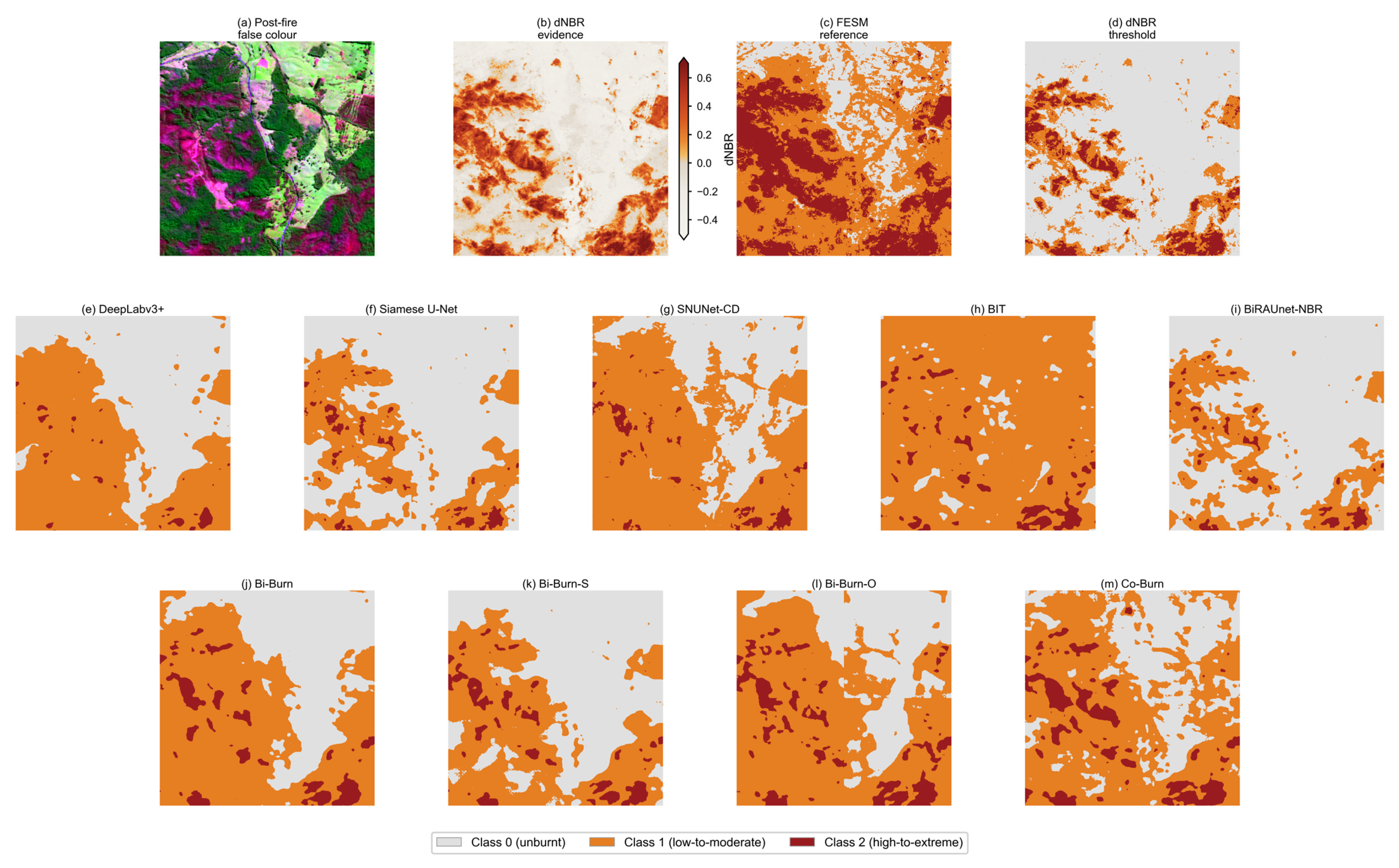
The three FESM classes form an ordered target with a conditional structure. Class 0 denotes the absence of mapped fire effects, whereas Classes 1 and 2 represent progressively greater canopy impact. This target structure motivates an explicit bi-temporal change input and a conditional severity output. Burn severity is also interpreted relative to the pre-fire condition, which motivates direct comparison of pre- and post-fire observations [12]. In a reflectance-only formulation, the model must infer the relevant NIR-SWIR change relationship from the raw bi-temporal bands. A nominal multiclass head, meanwhile, predicts the unburned and severity classes as parallel alternatives without representing that severity grading is conditional on burn presence. Co-Burn supplies the pre-to-post contrast as an input and uses burn presence in the final hierarchical class decision. The conditional ordinal head estimates burn presence first and grades severity only within burned pixels. These choices define two design axes: reflectance-only versus dNBR-anchored input and nominal multiclass versus conditional ordinal output.

Because deployment occurs at the level of complete fire events, evaluation uses the complete fire event as the unit of transfer [13,14]. The two Co-Burn design axes are evaluated through matched $2\times 2$ contrasts calculated separately for each external fire and training run. Four of the fourteen New South Wales fires are withheld in full for external testing and excluded from all stages of model development and selection. All learning-based methods follow common data splits, preprocessing, and inference procedures. External performance is assessed under pixel-pooled and event-mean aggregation, while fixed false-burn budgets and directional class-transition analysis resolve footprint expansion and ordered severity errors.

The main contributions are as follows.

1. Cross-event fire-severity mapping is formulated as burned-footprint delineation and ordered severity grading within the mapped footprint. This separates errors in where fire effects are mapped from errors in how the affected area is graded.

2. Co-Burn combines an explicit pre-to-post dNBR cue in the post-fire input with a conditional ordinal head that separates burn presence from high severity within burned pixels. Four matched variants are used to quantify the two design contrasts separately across the external fires.

3. Co-Burn is compared with nine other methods across 14 New South Wales wildfires, with four complete fires held out from training, configuration, and checkpoint selection. It ranks first under both pixel-pooled and event-mean external aggregation.

4. The evaluation uses matched false-burn-rate caps and event-level class-transition matrices to separate false expansion, burned-pixel omission, and severity reassignment. Burned mIoU alone does not distinguish these error directions.

2. Related Work

2.1. Spectral Foundations of Burn Severity Mapping

Forest-fire emissions from extratropical regions, including Australian temperate forests, have risen sharply in recent decades in response to fire-favourable weather [15]. Healthy vegetation typically has high reflectance in the NIR and lower reflectance in the SWIR. Fire-related canopy damage and vegetation moisture loss generally reduce the NIR response and increase the SWIR response relative to pre-fire conditions. The Normalised Burn Ratio (NBR) expresses this NIR-SWIR contrast as a single index, and dNBR measures the change in NBR between pre- and post-fire observations. Van Wagtendonk et al. [8] related dNBR to field-observed severity through the Composite Burn Index, giving the index its physical reading as fire-related spectral change.

NBR and its differenced form have also been widely used in operational burn-severity mapping. The US Monitoring Trends in Burn Severity (MTBS) programme combines NBR imagery with analyst interpretation to produce severity classes for a long-term fire archive [6]. In NSW, Australia, the Fire Extent and Severity Mapping (FESM) product uses Sentinel-2 imagery and supervised random-forest classification to map fire extent and severity [7,16]. Its classifier combines dNBR with other spectral-change indices and changes in vegetation cover. FESM provides the reference labels used in this study, with its classes derived from the joint information carried by several predictors. dNBR contributes directly to this target because it captures spectral responses associated with changes in canopy condition and vegetation moisture, although it does not determine the final classes on its own.

Pre-fire vegetation amount, vegetation type, surface background, burn pattern, and image acquisition timing can vary considerably among fire events. These factors affect both the range of dNBR values and their correspondence with severity classes. Miller and Thode [17] introduced RdNBR to reduce the influence of pre-fire vegetation amount on absolute dNBR, and Parks et al. [18] later proposed the relativized burn ratio. Roy et al. [19] and Soverel et al. [20] showed that similar fire effects can produce different index values across vegetation types, while similar values can correspond to different severity levels under different environmental conditions. Hislop et al. [21] further reported that post-fire acquisition timing alters the index response as canopy condition and vegetation moisture recover, particularly in resprouting Australian forests. These factors alter how a given dNBR value maps to a severity class, although dNBR itself still measures the pre-to-post NIR–SWIR change. A common threshold applies the same class boundaries to every fire, so the boundaries move relative to the severity they are meant to separate.

2.2. Bi-Temporal and Index-Guided Deep Learning

Single-image semantic segmentation was an early route for deep learning in fire mapping. U-Net, proposed by Ronneberger et al. [22], preserves local spatial detail through an encoder–decoder design with skip connections, and DeepLabv3+, proposed by Chen et al. [23], enlarges the receptive field with atrous convolution and multi-scale context. These general segmentation architectures were later adapted to pixel-wise burned-area and severity mapping, learning spatial patterns from texture, neighbourhood relationships, and boundary shape. With only a post-fire image, though, the network has no direct reference for the pre-fire state, and historical burn scars, terrain shadow, exposed soil, and water can be confused with the change caused by this fire.

Bi-temporal change-detection networks retain the pre-fire image as an explicit reference for interpreting the post-fire state. Shared-encoder Siamese models first compared paired features directly [24], and SNUNet-CD later introduced dense cross-scale fusion to preserve change information at multiple resolutions [25]. For wildfire burned-area mapping, BiAU-Net combined paired Sentinel-2 imagery with attention and a loss designed for class imbalance and mixed boundary pixels and was evaluated through cross-continent transfer experiments [26]. Transformer-based approaches followed a different representation strategy. BIT compresses the two dates into semantic tokens for long-range feature interaction [27], while Han et al. [28] fused multi-level Landsat features with environmental variables to map burned area and severity jointly. Severity was still decoded through nominal multiclass prediction, leaving its ordered structure outside the output formulation.

Recent burn-severity studies have incorporated explicit spectral-change indices alongside bi-temporal imagery. Hu et al. [9] compared post-fire imagery, burn indices, paired pre- and post-fire imagery, and paired imagery augmented with a dNBR-family index set under a fixed model setting. The pre-fire reference produced the larger improvement, while the index set provided a further gain. Wu et al. [11] developed BiRAUnet-NBR, which integrates paired imagery and dNBR-family layers within a residual-attention U-Net. The index-guided configuration improved mIoU under its original evaluation protocol. Both studies obtained their gains on the input side, with the nominal output held fixed throughout.

2.3. Ordinal and Hierarchical Modelling for Burn-Severity Labels

Fire-severity research has also examined how ordered damage levels should be represented at the output. Farasin et al. [29] proposed Double-Step U-Net, a sequential framework in which a binary U-Net first identifies burned pixels, and a separately trained regression U-Net then estimates an ordered damage level over the detected burned region. Monaco et al. [30] extended this framework and explicitly treated wildfire severity as an ordinal categorical variable. Their regression stage preserves the ordering of the severity scale by imposing larger penalties on predictions that lie farther from the reference level. Pelletier et al. [31] applied ordinal regression to relate remotely sensed burn-severity metrics to ground-based severity classes measured at forest inventory plots. These studies show that ordered severity has been considered explicitly in fire assessment. The sequential deep-learning approaches further separated burned-area identification from subsequent severity estimation.

Ordinal classification provides a discrete probabilistic framework for representing such ordering. Niu et al. [32] proposed OR-CNN, which decomposes an ordered target into binary decisions along the label scale. Cao et al. [33] introduced CORAL, adding rank-consistency constraints across these decisions. Shi et al. [34] proposed CORN, in which progression to a higher rank is expressed conditionally on the preceding rank having been reached. This conditional structure fits the present three-class target, where burn presence forms the first decision, and high-severity grading follows after burn presence has been established.

Recent pixel-wise burn-severity segmentation, including the studies of Hu et al. [9] and Wu et al. [11] reviewed above, has advanced mainly through temporal inputs, spectral indices, and network architecture while retaining nominal multiclass outputs. Co-Burn embeds burn-presence estimation and conditional high-severity grading within a shared bi-temporal pixel-wise model. The matched variants use common burn-presence supervision, while the conditional formulation uses the burn-presence prediction directly in hierarchical decoding before assigning the burned severity grade. The matched design compares nominal and conditional outputs under both reflectance-only and dNBR-anchored inputs. This design makes the output formulation an explicit experimental factor, with the matched variants sharing the backbone, training protocol, and burn-presence supervision.

2.4. Cross-Event Evaluation

Neighbouring pixels within the same fire often share strongly correlated spectral and spatial characteristics. When pixels or patches are randomly split within the same collection of fires, the training and test sets still share the same event backgrounds, and test samples may also lie close to the training areas. Such a split measures interpolation within familiar fire contexts rather than transfer to an independent fire event. Studies in spatial ecology and remote sensing have shown that ignoring spatial and hierarchical dependence produces optimistic performance estimates and can conceal substantial declines on spatially independent areas [13,14,35,36]. In fire-severity mapping specifically, Collins et al. [16] evaluated fire-severity classification using cross-validation across independent fires. A subsequent study by Collins et al. [37] used independent spatial cross-validation across a large multi-fire dataset and showed that classification performance was sensitive to the number of independent fires represented in training and the geographic source of the training samples. Van and Lee [38] further separated within-fire spatial generalisation, evaluated using Leave-One-Cluster-Out validation, from cross-fire transfer, evaluated using Leave-One-Fire-Out validation.

Because deployment concerns a fire that the model has not previously encountered, evaluation should be separated at the event level, with the complete fire event withheld. Event-level separation serves two roles in this study. Validation fires guide checkpoint selection, while a second set of complete events remains outside model development and provides the external transfer estimate. The external fires differ substantially in valid-pixel support. Pixel-pooled evaluation describes agreement over the combined valid FESM support of the external fires and gives events with more valid pixels greater weight. Event-mean evaluation first calculates burned mIoU for each fire and then averages the event scores, giving every fire equal weight.

3. Materials and Methods

3.1. Study Area and Fire-Event Dataset

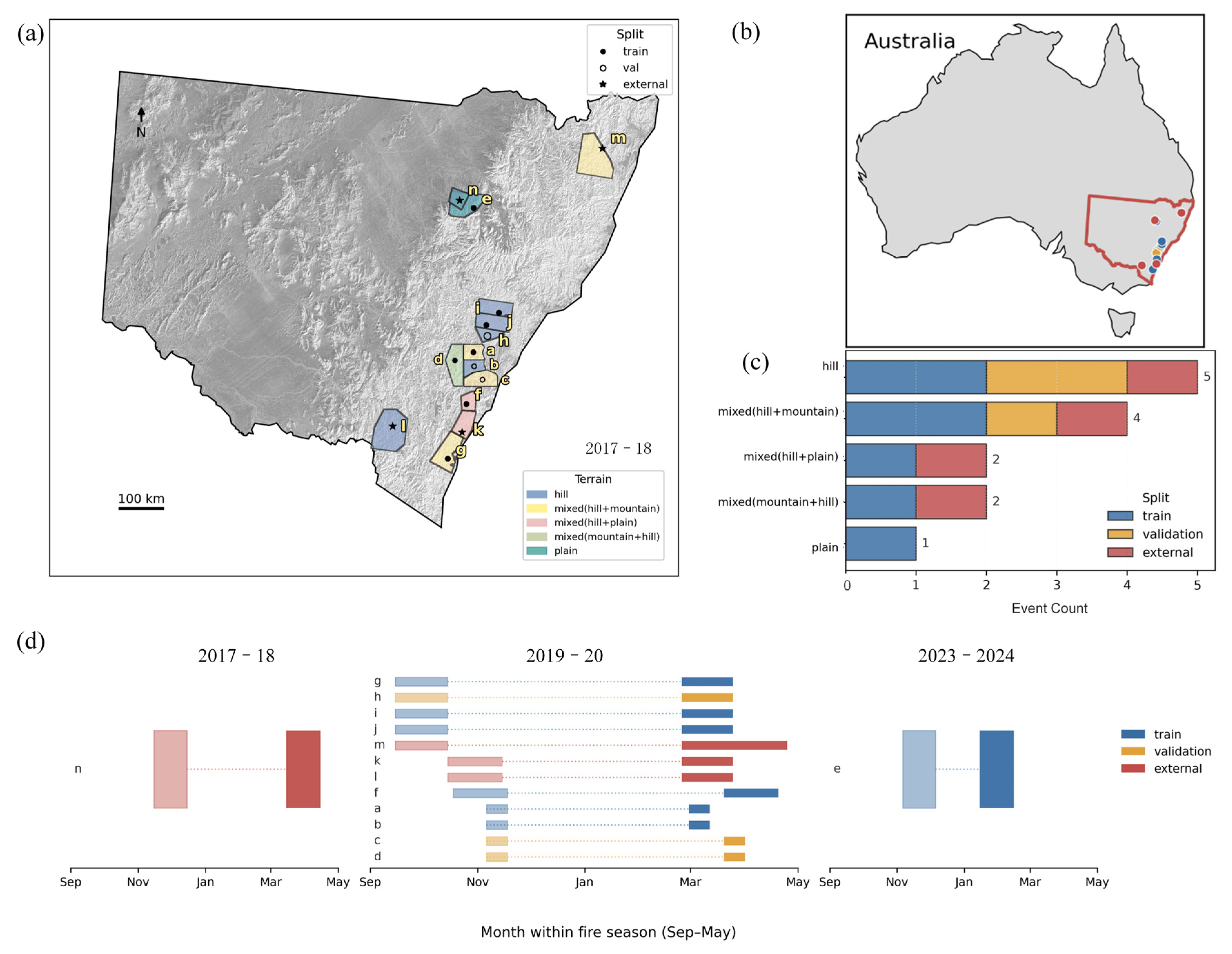
We assembled 14 forest wildfire events across NSW to evaluate cross-event transfer in bi-temporal burn-severity mapping. The events span the 2017–2018, 2019–2020, and 2023–2024 wildfire seasons. Each event is represented by paired Sentinel-2 pre-fire and post-fire observations, using either individual acquisitions or temporal composites, with reference labels from the NSW FESM product. Events were required to have more than 100 km² of mapped burned area, usable pre-fire and post-fire observations, available FESM labels, and predominantly forested cover. The archive contains approximately 20,000 km² of mapped burned area and extends from eastern coastal and tableland forests to the inland Pilliga region. Terrain composition was derived from Shuttle Radar Topography Mission (SRTM) elevation as an event-level descriptor and was not used as a model input. Its derivation is provided in Appendix A.1. Figure 1 shows the event locations, terrain settings, data splits, and fire-season coverage, and

Table 1. Metadata for the 14 New South Wales fire events with FESM reference labels. Event identifiers a–n are used consistently throughout this manuscript. Burned area was calculated from valid reference pixels labelled as burned classes 1 and 2 on the 10 m FESM grid. Terrain composition is a descriptive event-level summary. Its derivation is provided in Appendix A.1. Single dates denote screened individual Sentinel-2 acquisitions. Date ranges denote search/compositing windows, within which valid observations were combined band by band using the per-pixel median after SCL screening.

Event ID	Fire Event	Fire Season	Burned Area (km2)	Terrain Setting (Leading Classes, %)	Pre-Fire Date/Window	Post-Fire Date/Window	Split
a	Kanangra Walls	2019–2020	331.9	Mixed; Mountain/highland 39.7%, Hill 38.7%	6 November 2019	29 February 2020	train
b	Wolgan Valley	2019–2020	144.1	Mixed; Hill 48.2%, Mountain/highland 42.2%	6 November 2019	29 February 2020	train
c	Wollondilly River	2019–2020	247.8	Mixed; Hill 50.2%, Mountain/highland 39.0%	6 November 2019	20 March 2020	validation
d	Wombeyan Caves	2019–2020	153.4	Hill (62.6%)	6 November 2019	20 March 2020	validation
e	Pilliga East	2023–2024	699.8	Plain (98.4%)	6 November 2023–6 December 2023	15 January 2024–15 February 2024	train
f	Bundanoon	2019–2020	1152.5	Mixed; Hill 46.4%, Plain 28.5%	18 October 2019–18 November 2019	20 March 2020–20 April 2020	train
g	Araluen	2019–2020	2943.9	Mixed; Hill 52.9%, Mountain/highland 28.5%	15 September 2019–15 October 2019	25 February 2020–25 March 2020	train
h	Lithgow	2019–2020	1012.6	Hill (61.1%)	15 September 2019–15 October 2019	25 February 2020–25 March 2020	validation
i	Mellong	2019–2020	2209.3	Hill (60.0%)	15 September 2019–15 October 2019	25 February 2020–25 March 2020	train
j	Putty	2019–2020	1882.7	Hill (64.2%)	15 September 2019–15 October 2019	25 February 2020–25 March 2020	train
k	Nerriga	2019–2020	1976.3	Mixed; Hill 51.2%, Plain 34.1%	15 October 2019–15 November 2019	25 February 2020–25 March 2020	external
l	Talbingo	2019–2020	3421.7	Hill (60.2%)	15 October 2019–15 November 2019	25 February 2020–25 March 2020	external
m	Grafton	2019–2020	3160.9	Mixed; Hill 52.9%, Mountain/highland 29.0%	15 September 2019–15 October 2019	25 March 2020–25 April 2020	external
n	Pilliga West	2017–2018	583.9	Plain (97.2%)	15 November 2017–15 December 2017	15 March 2018–15 April 2018	external

lists the event-level metadata.

To prevent spatial data leakage, data partitioning was executed strictly by complete events, keeping the training, validation, and external test sets with no fire shared between the three sets. The split was fixed before model development with distinct roles. The training set was selected to cover the main temporal, geographic, terrain, fire-size, and image-acquisition variation. Seven events were used for training $\left\{a,b,e,f,g,i,j\right\}$. They span two main fire seasons, cover diverse terrains, and are distributed broadly across NSW. Three complete fires not used for training $\left\{c,d,h\right\}$ were assigned to validation. Four additional complete fires $\left\{k,l,m,n\right\}$ were reserved for external testing. No external event contributed to model fitting, configuration selection, checkpoint selection, or the fixed operating rules used in the main benchmark.

Pilliga East (e) and Pilliga West (n) are separate fires from different fire seasons, although their mapped burned extents partially overlap within the Pilliga region. We also report a robustness analysis excluding event n in Appendix A.5.

3.2. Sentinel-2 Imagery, dNBR, and Reference Labels

3.2.1. Sentinel-2 Acquisition and Preprocessing

Pre-fire and post-fire Sentinel-2 Level-2A surface-reflectance products [39] were obtained from the Copernicus Data Space Ecosystem and prepared on a common geographic grid (EPSG:4326, WGS 84) with an approximate 10 m spacing over each event. We used bands B2, B3, B4, B8, B11, and B12. The two SWIR bands, B11 and B12, were resampled from 20 m to the common grid by nearest-neighbour interpolation. All six bands were therefore aligned before index calculation and model input construction. The FESM reference and its valid mask were also resampled to the pre-fire grid by nearest-neighbour interpolation.

Cloud and non-target pixels were screened with the Sentinel-2 scene classification layer (SCL). We discarded cloud shadow, water, medium-probability cloud, high-probability cloud, thin cirrus pixels (SCL classes 3, 6, 8, 9, and 10), and saturated or defective pixels (SCL class 1). A pixel observation was retained only when all six bands were present after this screening. The pre-fire and post-fire stacks shared the same event grid, so no additional image-to-image co-registration was applied.

Each pre-fire and post-fire image source followed the date or acquisition window listed in Table 1. Most windows covered approximately one month. When Table 1 lists a single acquisition, the masked image from that date was used. When it lists a window, valid observations within that window were composited band by band using the per-pixel median. For Grafton, the post-fire compositing search continued through 25 April 2020. No temporal interpolation or gap filling was applied.

The final analysis mask was the intersection of three components: the valid pre-fire image or composite, the valid post-fire image or composite, and the valid FESM label mask. Only pixels inside this common mask were used for model fitting, dNBR calculation, prediction evaluation, confusion matrices, and false-burn-rate calculation. Pixels outside the common mask were treated as missing data and were not counted as Class 0.

3.2.2. dNBR Computation

For each date, NBR was computed from Sentinel-2 B8 and B12, the band pair used in the FESM workflow [7], as

$$\mathrm{N}\mathrm{B}\mathrm{R}={\displaystyle \frac{B_8-B_{12}}{B_8+B_{12}+\epsilon }},$$

(1)

where $\epsilon =1\times {10}^{-6}$ is a small numerical constant. The bi-temporal index dNBR was calculated pixel-wise from the unnormalised Level-2A surface-reflectance bands as

$$\mathrm{d}\mathrm{N}\mathrm{B}\mathrm{R}={\mathrm{N}\mathrm{B}\mathrm{R}}_{\mathrm{p}\mathrm{r}\mathrm{e}}-{\mathrm{N}\mathrm{B}\mathrm{R}}_{\mathrm{p}\mathrm{o}\mathrm{s}\mathrm{t}}.$$

(2)

This B8/B12 convention follows the FESM workflow [7]. For variants that use dNBR as an additional input channel, the resulting layer was clipped to $\left[-1,1\right]$ and retained on this index scale without z-score normalisation. Clipping bounded residual extreme values while preserving zero as the no-NBR-change point. The six reflectance bands from each date were first normalised channel-wise using training-set means and standard deviations. The seventh channel was then appended, with clipped dNBR to the post-fire stack and an exact zero layer to the pre-fire stack. It provides the matched input shape required by the tied encoder. Neither seventh channel was subsequently rescaled. The same construction was used during training and inference. Bi-Burn-S and Co-Burn received the clipped layer, whereas the event-level raw-dNBR summaries in

Table A4. Event-level raw-dNBR context of the FESM-derived Class-1 and Class-2 boundary across seven evaluation events.

Event ID	Split	HCR	$1-\mathbf{A}\mathbf{U}\mathbf{C}$	${\mathsf{\tau }}_{\mathit{r}}$
c	Validation	0.868	0.074	0.324
d	Validation	0.903	0.046	0.330
h	Validation	0.832	0.134	0.419
k	External	0.824	0.088	0.314
l	External	0.856	0.081	0.368
m	External	0.418	0.409	0.115
n	External	0.841	0.055	0.218

were calculated from unclipped dNBR on the same paired valid-pixel support.

3.2.3. FESM Reference Labels and Three-Class Severity Formulation

Reference labels were obtained from the New South Wales FESM product [7], a publicly released Sentinel-2-based product for state-level post-fire assessment. FESM defines five severity classes: unburnt, low, moderate, high, and very high (extreme). The FESM labels and associated valid mask were transferred to the same 10 m grid by nearest-neighbour resampling, preserving their discrete values.

For this study, the five FESM classes were aggregated into an ordered three-class target. Class 0 corresponds to unburnt, Class 1 combines low and moderate severity, and Class 2 combines high to extreme severity. This aggregation follows the canopy-condition progression represented by the FESM scheme: low and moderate severity span burnt understorey with an unburnt or partly scorched canopy, whereas high and extreme severity span complete canopy scorch through partial or full canopy consumption. The FESM-derived three-class map was used as the operational remote-sensing reference for model fitting and evaluation. All reported metrics quantify agreement with this target.

The aggregation also reduces distinctions that are difficult to maintain consistently in a three-class spectral learning task. In the Sentinel-2 FESM accuracy assessment, moderate severity had the lowest class-specific accuracy among the five original classes, and disagreements between Sentinel-2 and Landsat FESM outputs commonly occurred between adjacent severity categories, including low versus moderate and high versus extreme [40]. The resulting target retains the ordered relation ($0<1<2$) used by the conditional ordinal head while providing broader support for model fitting and event-level evaluation.

Pixels outside the valid FESM mask were excluded from training and evaluation. Class 0 denotes reference-unburnt pixels within the mapped FESM extent. Burn-presence predictions introduced in Section 3.3 are interpreted within this valid extent. The reported metrics therefore describe performance within the valid FESM reference extent and do not evaluate background outside that extent. False-burn rate (FBR) is reported separately in Section 3.7 to quantify predictions that assign burned classes to reference Class-0 pixels.

3.3. Problem Formulation

We formulate fire-severity mapping as pixel-wise ordinal classification within the valid FESM reference extent defined in Section 3.2.3. Let $X^{\mathrm{p}\mathrm{r}\mathrm{e}}, X^{\mathrm{p}\mathrm{o}\mathrm{s}\mathrm{t}}\in {\mathbb{R}}^{H\times W\times 6}$ denote the z-score-normalised six-band reflectance stacks, respectively, while $D\in {\mathbb{R}}^{H\times W\times 1}$ refers to the clipped dNBR layer. Let Ω denote the set of valid reference pixels. For each pixel $i\in \mathsf{\Omega }$, the target label $y_i\in \left\{0,1,2\right\}$ corresponds to unburnt land within the mapped extent, low-to-moderate severity, and high-to-extreme severity.

The input factor distinguishes reflectance-only inputs from dNBR-anchored inputs. For reflectance-only models, the bi-temporal input is

$$x_0=\left(X^{\mathrm{p}\mathrm{r}\mathrm{e}},X^{\mathrm{p}\mathrm{o}\mathrm{s}\mathrm{t}}\right).$$

(3)

For dNBR-anchored models, an additional channel is appended to each temporal branch,

$$x_D=\left(\mathrm{c}\mathrm{a}\mathrm{t}(X^{\mathrm{p}\mathrm{r}\mathrm{e}},\mathbf{0}),\mathrm{c}\mathrm{a}\mathrm{t}(X^{\mathrm{p}\mathrm{o}\mathrm{s}\mathrm{t}},D)\right)$$

(4)

where $\mathbf{0}\in {\mathbb{R}}^{\mathrm{H}\times \mathrm{W}\times 1}$ is a zero-valued layer. $\mathrm{c}\mathrm{a}\mathrm{t}\left(\cdot \right)$ denotes concatenation along the channel dimension. Both branches therefore contain seven channels, with dNBR supplied only to the post-fire branch.

The output axis compares a nominal severity formulation with a conditional ordinal formulation. Both formulations share the same decoded feature map and the same burn-presence head, which predicts the probability in Equation (5) and is supervised in both. In the nominal variants this output is an auxiliary signal, while a separate three-class softmax predicts $P(y_i=c\mid x)$ for $c\in \{0,1,2\}$, and the final map is the per-pixel argmax of that branch. In the conditional variants the burn-presence probability is used directly as the first step of the hierarchical decision in Equations (5)–(8):

$$p_b(i)=P(y_i>0|x).$$

(5)

A second output predicts high severity conditional on burn presence:

$$p_h(i)=P(y_i=2|y_i>0,x).$$

(6)

These two combine into the three-class distribution

$$P(y_i=0|x)=1-p_b(i)$$

(7)

$$P(y_i=1|x)=p_b\left(1-p_h\left(i\right)\right)$$

(8)

$$P(y_i=2|x)=p_b\left(i\right)p_h\left(i\right).$$

(9)

At inference, the conditional variants use a hierarchical operating rule

$${\widehat{y}}_i=\{\begin{array}{c}0 if p_b(i)\le {\tau }_b \\ 1 if{p}_b(i)>{\tau }_b \mathrm{and} p_h(i)\le {\tau }_h\\ 2 if p_b(i)>{\tau }_b \mathrm{and} p_h(i)>{\tau }_h\end{array}.$$

(10)

This rule keeps burn-presence assignment under direct control of ${\tau }_b$ and then applies conditional severity grading within the mapped burned extent. At the fixed benchmark operating point, the conditional variants use ${\tau }_b={\tau }_h=0.5$.

Let ${\mathrm{b}}_{\mathrm{i}}=\mathbb{1}(y_i>0)$ denote the binary burn-presence target. Let ${\mathsf{\Omega }}_{\mathrm{b}\mathrm{a}\mathrm{t}\mathrm{c}\mathrm{h}}$ contain all valid pixel instances in the current batch, and let ${\mathsf{\Omega }}_n$ denote the valid pixels of its $n$-th tile, with $T$ tiles per batch.

All four matched variants share the same burn-presence objective, the sum of a masked binary cross-entropy (BCE) term ${\mathcal{L}}_{\mathrm{B}\mathrm{C}\mathrm{E}}$ and a soft Dice ${\mathcal{L}}_{\mathrm{D}\mathrm{i}\mathrm{c}\mathrm{e}}$ term as

$${\mathcal{L}}_{\mathrm{b}\mathrm{i}\mathrm{n}}={\mathcal{L}}_{\mathrm{B}\mathrm{C}\mathrm{E}}+{\mathcal{L}}_{\mathrm{D}\mathrm{i}\mathrm{c}\mathrm{e}}$$

(11)

$${\mathcal{L}}_{\mathrm{B}\mathrm{C}\mathrm{E}}=-{\displaystyle \frac{1}{\left|{\mathsf{\Omega }}_{\mathrm{b}\mathrm{a}\mathrm{t}\mathrm{c}\mathrm{h}}\right|}}\sum _{i\in {\mathsf{\Omega }}_{\mathrm{b}\mathrm{a}\mathrm{t}\mathrm{c}\mathrm{h}}}\left[b_i\mathrm{l}\mathrm{o}\mathrm{g}{p}_b\left(i\right)+\left(1-b_i\right)\mathrm{l}\mathrm{o}\mathrm{g}\left(1-p_b\left(i\right)\right)\right]$$

(12)

$${\mathcal{L}}_{\mathrm{D}\mathrm{i}\mathrm{c}\mathrm{e}}=1-{\displaystyle \frac{1}{T}}{\displaystyle \sum _{n=1}^T}{\displaystyle \frac{2{\sum }_{i\in {\mathsf{\Omega }}_n}{p}_b\left(i\right)\hspace{0.17em}{b}_i+\delta }{{\sum }_{i\in {\mathsf{\Omega }}_n}{p}_b{\left(i\right)}^2+{\sum }_{i\in {\mathsf{\Omega }}_n}{b}_i^2+\delta }}$$

(13)

with $\mathsf{\delta }=1\times {10}^{-6}$. The BCE term is pooled over all valid pixels in the batch, whereas the Dice term is calculated separately for each tile and then averaged over the $T$ tiles.

The two formulations differ in the severity term. For the nominal variants, ${\mathcal{L}}_{\mathrm{s}\mathrm{e}\mathrm{v}}$ is the mean weighted categorical cross-entropy over ${\mathsf{\Omega }}_{\mathrm{b}\mathrm{a}\mathrm{t}\mathrm{c}\mathrm{h}}$, with class weights 1.0, 2.0, and 1.0 for Classes 0, 1, and 2. For the conditional variants, ${\mathcal{L}}_{\mathrm{h}\mathrm{i}\mathrm{g}\mathrm{h}}$ is the mean binary cross-entropy over pixels $i\in {\mathsf{\Omega }}_{\mathrm{b}\mathrm{a}\mathrm{t}\mathrm{c}\mathrm{h}}$ with $y_i>0,$ using $1(y_i=2)$ as the target.

$${\mathcal{L}}_{\mathrm{n}\mathrm{o}\mathrm{m}}={\lambda }_b\hspace{0.17em}{\mathcal{L}}_{\mathrm{b}\mathrm{i}\mathrm{n}}+{\lambda }_s\hspace{0.17em}{\mathcal{L}}_{\mathrm{s}\mathrm{e}\mathrm{v}}$$

(14)

$${\mathcal{L}}_{\mathrm{o}\mathrm{r}\mathrm{d}}={\lambda }_b\hspace{0.17em}{\mathcal{L}}_{\mathrm{b}\mathrm{i}\mathrm{n}}+{\lambda }_h\hspace{0.17em}{\mathcal{L}}_{\mathrm{h}\mathrm{i}\mathrm{g}\mathrm{h}}.$$

(15)

The common binary coefficient was ${\mathsf{\lambda }}_{\mathrm{b}}=1.0$. The active severity coefficient was ${\mathsf{\lambda }}_{\mathrm{s}}=0.5$ for nominal variants and ${\mathsf{\lambda }}_{\mathrm{h}}=0.5$ for conditional variants. The nominal variants therefore combine the shared burn-presence objective with weighted three-class severity supervision over all valid pixels, whereas the conditional variants replace that term with high-severity supervision restricted to reference-burned pixels.

Combining the input axis in Equations (3) and (4) with the nominal and conditional output formulations defines four matched variants: Bi-Burn ($x_0$, nominal), Bi-Burn-S ($x_D$, nominal), Bi-Burn-O ($x_0$, conditional), and Co-Burn ($x_D$, conditional). S denotes dNBR spectral anchoring, and O denotes the conditional ordinal formulation. Co-Burn combines both. Section 3.4 describes the shared backbone. Section 3.6.2 defines the factorial decomposition of these four variants, and Section 3.6.3 varies ${\tau }_b$ across $\left[0,1\right]$ while holding ${\tau }_h=0.5$ to trace the false-burn-rate and burned-mIoU trade-off.

3.4. Co-Burn Architecture and $2\times 2$ Factorial Design

3.4.1. Shared Bi-Temporal Backbone

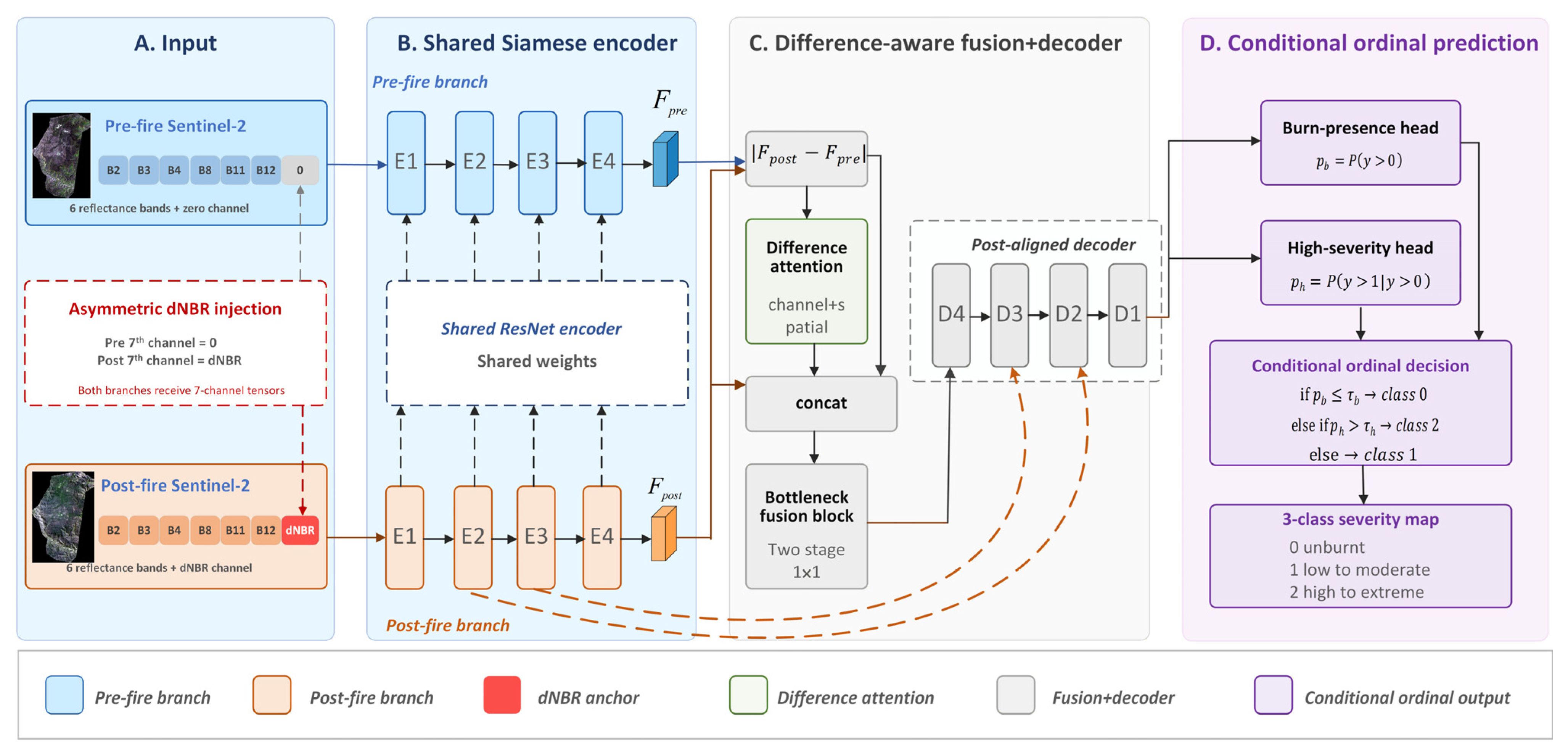
All variants use the same bi-temporal encoder–decoder topology, shown in Figure 2. Within each model, the pre-fire and post-fire inputs are processed by two ResNet-18 encoder branches with shared weights, operating on normalised inputs (Section 3.2.2). Bi-temporal information is aggregated at the deepest encoder bottleneck. The absolute feature difference $|F_{post}^{\left(4\right)}-F_{pre}^{\left(4\right)}|$ between the two branches is reweighted by a channel-and-spatial attention module [41] applied to the difference map. It is then concatenated with the post-fire bottleneck feature and compressed by a two-stage $1\times 1$ convolutional fusion block.

Figure 2. Co-Burn architecture. Pre-fire and post-fire inputs are encoded by tied ResNet-18 branches; the bottleneck difference is attention-reweighted, fused with the post-fire feature, and decoded through post-fire multi-scale skip connections. In Co-Burn, clipped dNBR is appended to the post-fire input with a zero channel on the pre-fire side. The other three factorial variants are obtained by switching the input and/or output formulation as specified in Table 2. Solid black arrows denote the main forward data flow through the encoder–fusion–decoder pipeline; dashed black arrows link the pre-fire and post-fire encoder branches to the shared ResNet encoder, indicating tied weights; orange dashed arrows denote the post-fire multi-scale skip connections feeding into the decoder.

Figure 2. Co-Burn architecture. Pre-fire and post-fire inputs are encoded by tied ResNet-18 branches; the bottleneck difference is attention-reweighted, fused with the post-fire feature, and decoded through post-fire multi-scale skip connections. In Co-Burn, clipped dNBR is appended to the post-fire input with a zero channel on the pre-fire side. The other three factorial variants are obtained by switching the input and/or output formulation as specified in Table 2. Solid black arrows denote the main forward data flow through the encoder–fusion–decoder pipeline; dashed black arrows link the pre-fire and post-fire encoder branches to the shared ResNet encoder, indicating tied weights; orange dashed arrows denote the post-fire multi-scale skip connections feeding into the decoder.

Table 2. Four variants in the matched $2\times 2$ design. $x_0$ denotes paired six-band pre-fire and post-fire reflectance inputs. $x_D$ represents the corresponding seven-channel inputs with a zero-valued seventh channel in the pre-fire branch and clipped dNBR in the post-fire branch.

Variant	Input	Output Formulation
Bi-Burn	$x_0$	Nominal
Bi-Burn-S	$x_D$	Nominal
Bi-Burn-O	$x_0$	Conditional
Co-Burn	$x_D$	Conditional

Table 2. Four variants in the matched $2\times 2$ design. $x_0$ denotes paired six-band pre-fire and post-fire reflectance inputs. $x_D$ represents the corresponding seven-channel inputs with a zero-valued seventh channel in the pre-fire branch and clipped dNBR in the post-fire branch.

Variant	Input	Output Formulation
Bi-Burn	$x_0$	Nominal
Bi-Burn-S	$x_D$	Nominal
Bi-Burn-O	$x_0$	Conditional
Co-Burn	$x_D$	Conditional

3.4.2. Post-Fire dNBR Injection

dNBR is carried by the post-fire branch because the decoder receives its multi-scale skip features from that branch. The explicit change cue can therefore propagate through the post-fire skip pathways as well as the bottleneck, while the pre-fire reflectance remains the reference observation. The construction of the seventh channel is described in Section 3.2.2.

3.4.3. Factorial Variants on the Shared Backbone

All four variants share this backbone and differ only in input channels and output formulation as set out in Table 2. Fusion, decoder, training schedule, and evaluation settings are matched across them, and so is the burn-presence objective in Equations (11)–(13). The output axis replaces nominal three-class severity prediction and argmax decoding with conditional high-severity prediction on reference-burned pixels and hierarchical decoding. The factorial estimate in Section 3.6.2 therefore applies to the conditional ordinal formulation as a whole.

3.5. Comparison Methods and Training Protocol

3.5.1. Comparison Methods

We compared the four matched variants introduced in Section 3.4 with six reference methods. As a deterministic spectral reference, the dNBR baseline used two fixed cut points, 0.10 and 0.44, drawn from the example dNBR severity ranges of the FIREMON Landscape Assessment scheme [42] and simplified to the three-class structure used here. It assigned Class 0 for dNBR < 0.10, Class 1 for 0.10 ≤ dNBR < 0.44, and Class 2 for dNBR ≥ 0.44. The same thresholds were applied globally to all events and were not fitted to the validation or external fires. This baseline therefore served as a fixed spectral reference rather than an event-calibrated classifier. DeepLabv3+ [23] served as an early-fusion segmentation baseline, receiving the concatenated pre-fire and post-fire six-band reflectance stacks as a 12-channel input. Siamese U-Net [24] represented the basic shared-encoder bi-temporal design. SNUNet-CD [25] added dense cross-scale fusion, while BIT [27] provided a Transformer-based comparison. BiRAUnet-NBR was included as the most direct fire-specific input-side baseline. It combines pre-fire and post-fire imagery with dNBR-family layers in a residual-attention architecture and retains a nominal multiclass output. To maintain a common preprocessing protocol, the histogram-matching step used in the original BiRAUnet-NBR study was not applied. All trainable baselines were configured for the three FESM severity classes. With the four matched variants, they formed the ten-method benchmark.

All trainable methods used the same event split, Sentinel-2 preprocessing, valid-pixel masks, and reference labels. Input construction followed the requirements of each architecture.

3.5.2. Training Protocol

The four factorial variants and the reference networks other than BiRAUnet-NBR were optimised with AdamW. BiRAUnet-NBR used its own model-specific trainer. Training was performed on pre-extracted tiles after channel-wise z-score normalization with statistics calculated from the training set.

Training used 2541 non-overlapping $256\times 256$ tiles extracted from the seven training fires. Tiles were retained when at least 50% of their pixels were valid. No minimum burned-pixel requirement was imposed, so purely Class-0 tiles were retained. A total of 491 training tiles contained no valid Class-1 or Class-2 pixels. Training batches were formed by uniform shuffling over the retained tile set, without event balancing, class-aware sampling, or oversampling. The same training-event support, tile lists, and normalization statistics were used by all trainable methods. Across the retained training pixels, Classes 0, 1, and 2 accounted for 32.00%, 33.81%, and 34.19% of the valid reference pixels, respectively. Because batches were formed by tile-uniform shuffling, each event’s sampling probability was proportional to its number of retained tiles.

Table A6. Per-event training-tile construction and sampling share. Candidate tiles were generated on a non-overlapping 256 × 256 grid. Tiles with less than 50% valid pixels were excluded. Sampling share is the fraction of the 2541 retained training tiles contributed by each event.

Event ID	Candidate Tiles	Retained Tiles	Excluded Tiles	Pure Class-0 Tiles	Sampling Weight (%)
a	96	64	32	0	2.52
b	114	40	74	1	1.57
e	1440	626	814	457	24.64
f	357	241	116	1	9.48
g	1152	654	498	7	25.74
i	481	474	7	10	18.65
j	444	442	2	15	17.39
Total	4084	2541	1543	491	100.00

reports the candidate and retained tile counts, purely Class-0 tiles, and implied sampling weight for each training fire. No data augmentation was applied in the reported training runs. Validation used 332 pre-extracted $256\times 256$ tiles from events c, d, and h.

Each trainable model was trained independently using seeds 42, 99, 1998, 2026, and 3531. For each run, the checkpoint with the highest validation burned mIoU was retained for external evaluation. All seed-based analyses used the same five runs. Qualitative figures use seed-42 predictions consistently across the trainable models. The dNBR threshold baseline was deterministic once its class thresholds were fixed. Full-event rasters were processed with $256\times 256$ sliding windows and a stride of 128 pixels. Predictions in overlapping regions were combined using raised-cosine weights. No morphological or other spatial post-processing was applied before metric calculation.

DeepLabv3+, Siamese U-Net, SNUNet-CD, and BIT used the nominal objective in Equation (14), including the shared burn-presence output and its BCE-Dice term. Their reported three-class maps were decoded from the nominal softmax output by argmax. BiRAUnet-NBR used its model-specific trainer and a differentiable mean-IoU objective computed from softmax probabilities over all three classes on valid pixels, with $\mathsf{\epsilon }={10}^{-7}$. It did not use the common burn-presence output or label smoothing. Its preprocessing, checkpoint criterion, and external evaluation protocol were otherwise matched to the benchmark protocol.

Table 3. Model configurations and training settings.

Model	Train Patch	Batch	LR	WD	Epochs	Params (M)
DeepLabv3+	256 × 256	4	1 × 10−4	1 × 10−4	60	40.4
Siamese U-Net	256 × 256	4	1 × 10−4	1 × 10−4	50	1.8
SNUNet-CD	256 × 256	4	1 × 10−4	1 × 10−4	80	13.2
BIT	256 × 256	4	5 × 10−5	5 × 10−2	60	13.3
BiRAUnet-NBR *	256 × 256	32	1 × 10−3	0	50	6.4
Bi-Burn	256 × 256	4	1 × 10−4	1 × 10−4	50	13.9
Bi-Burn-S	256 × 256	4	1 × 10−4	1 × 10−4	50	13.9
Bi-Burn-O	256 × 256	4	1 × 10−4	1 × 10−4	50	13.9
Co-Burn	256 × 256	4	1 × 10−4	1 × 10−4	50	13.9

* Histogram matching was omitted to keep the preprocessing protocol common across all models.

summarizes the training settings and parameter counts for all trainable methods. All learned models were implemented in PyTorch 2.5.1 (Python 3.11.7) and trained on an NVIDIA RTX 2000 Ada Generation Laptop GPU (NVIDIA Corporation, Santa Clara, CA, USA).

3.6. Evaluation Protocols

3.6.1. Complete-Event Benchmark and Dual Aggregation

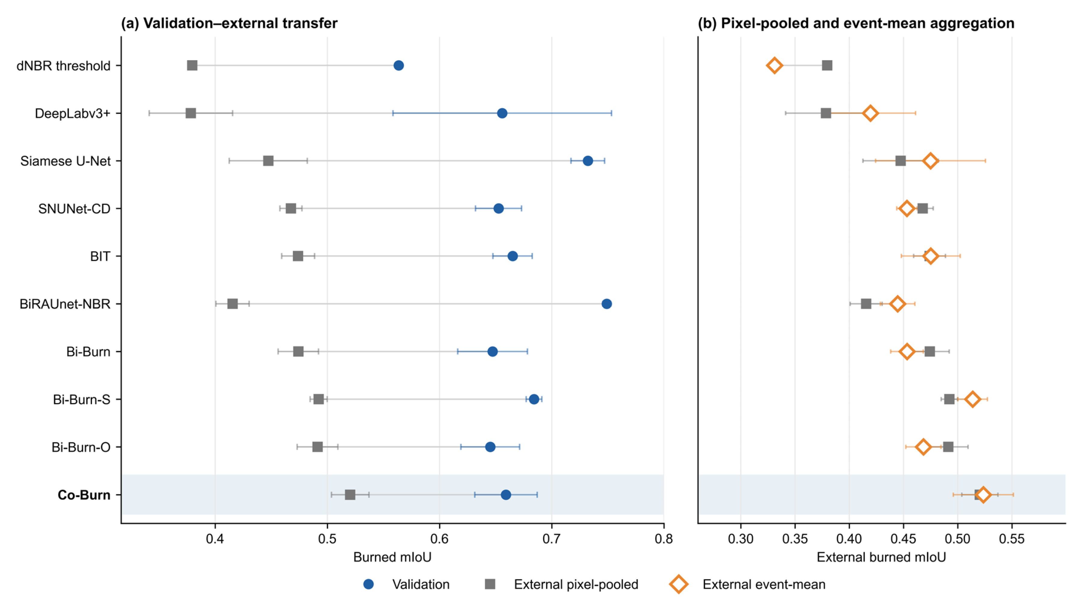
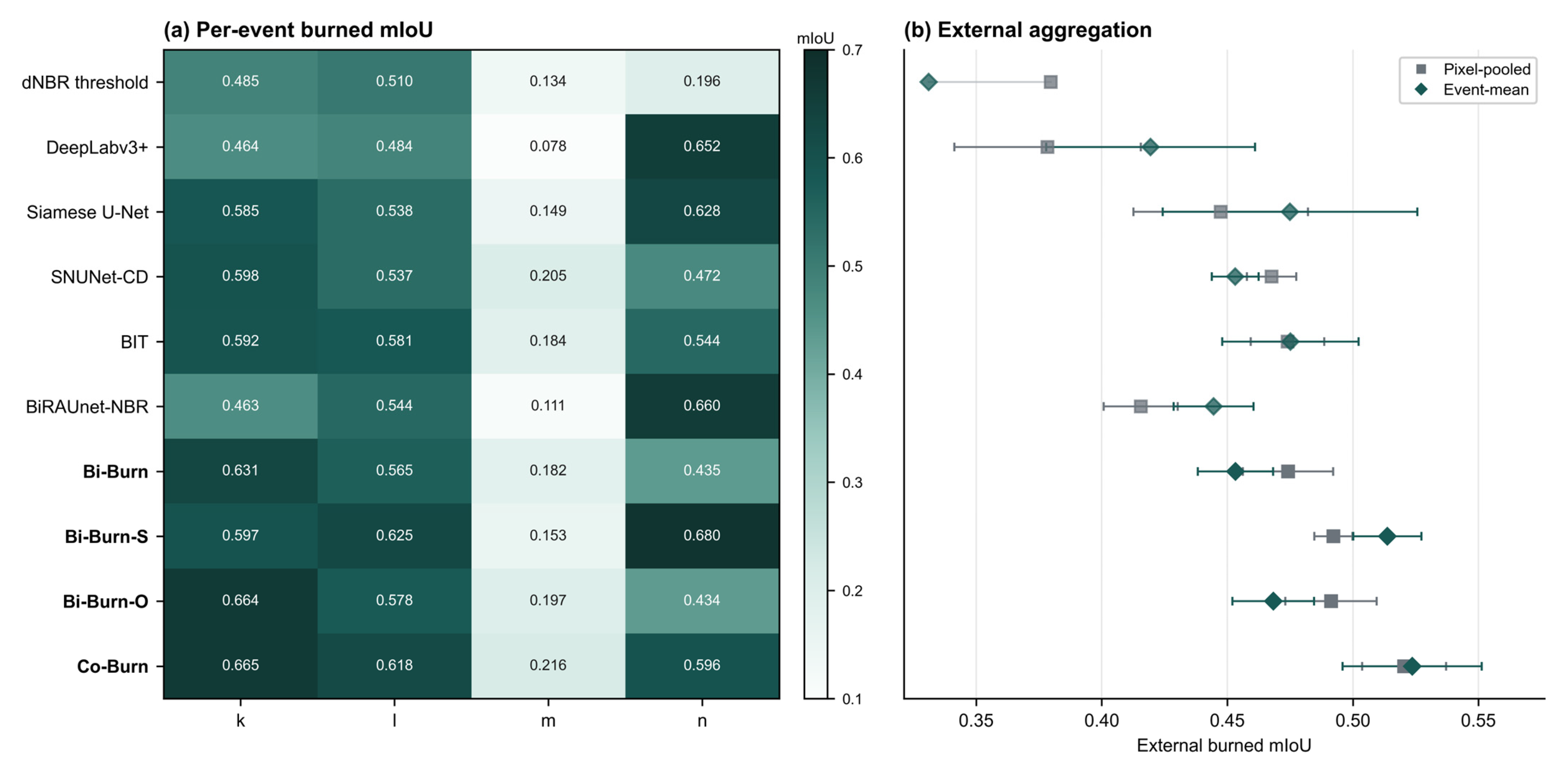
The ten methods were evaluated on external events k, l, m, and n, all of which were excluded from training and validation. Predictions were compared with the FESM-derived three-class reference within each event’s valid extent. External performance was prespecified under pixel-pooled and event-mean aggregation, as defined in Equations (23) and (24), with burned mean intersection-over-union (mIoU) as the primary metric.

3.6.2. Event-Primary Matched Factorial Analysis

The four variants in Table 2 share the same backbone, training configuration, and evaluation protocol. They form a matched $2\times 2$ design in which the input axis controls dNBR anchoring, and the output axis controls the nominal or conditional ordinal formulation.

For external fire $r$ and training run $s$, let $A_{r,s}$, $S_{r,s}$, $O_{r,s}$, and $C_{r,s}$ denote the outcome for Bi-Burn, Bi-Burn-S, Bi-Burn-O, and Co-Burn, respectively. The dNBR contrast is

$${∆}_{r,s}^{\mathrm{d}\mathrm{N}\mathrm{B}\mathrm{R}}={\displaystyle \frac{\left(S_{r,s}-A_{r,s}\right)+\left(C_{r,s}-O_{r,s}\right)}{2}}.$$

(16)

The conditional ordinal contrast is

$${∆}_{r,s}^{\mathrm{o}\mathrm{r}\mathrm{d}}={\displaystyle \frac{\left(O_{r,s}-A_{r,s}\right)+\left(C_{r,s}-S_{r,s}\right)}{2}}.$$

(17)

The interaction is defined as

$${∆}_{r,s}^{\mathrm{i}\mathrm{n}\mathrm{t}}=C_{r,s}-S_{r,s}-O_{r,s}+A_{r,s}).$$

(18)

These contrasts were calculated separately for every external fire and matched training run for burned mIoU and false-burn rate. The five run-level contrasts were then averaged within each fire. The four fire-level effects are reported individually and summarized by their equal-event mean. Sensitivity to any single external fire is summarized by the range of the four leave-one-fire-out means, each calculated after omitting one fire and averaging the remaining three. Training-run standard deviations describe variation due to training stochasticity.

3.6.3. Operating-Point Analysis

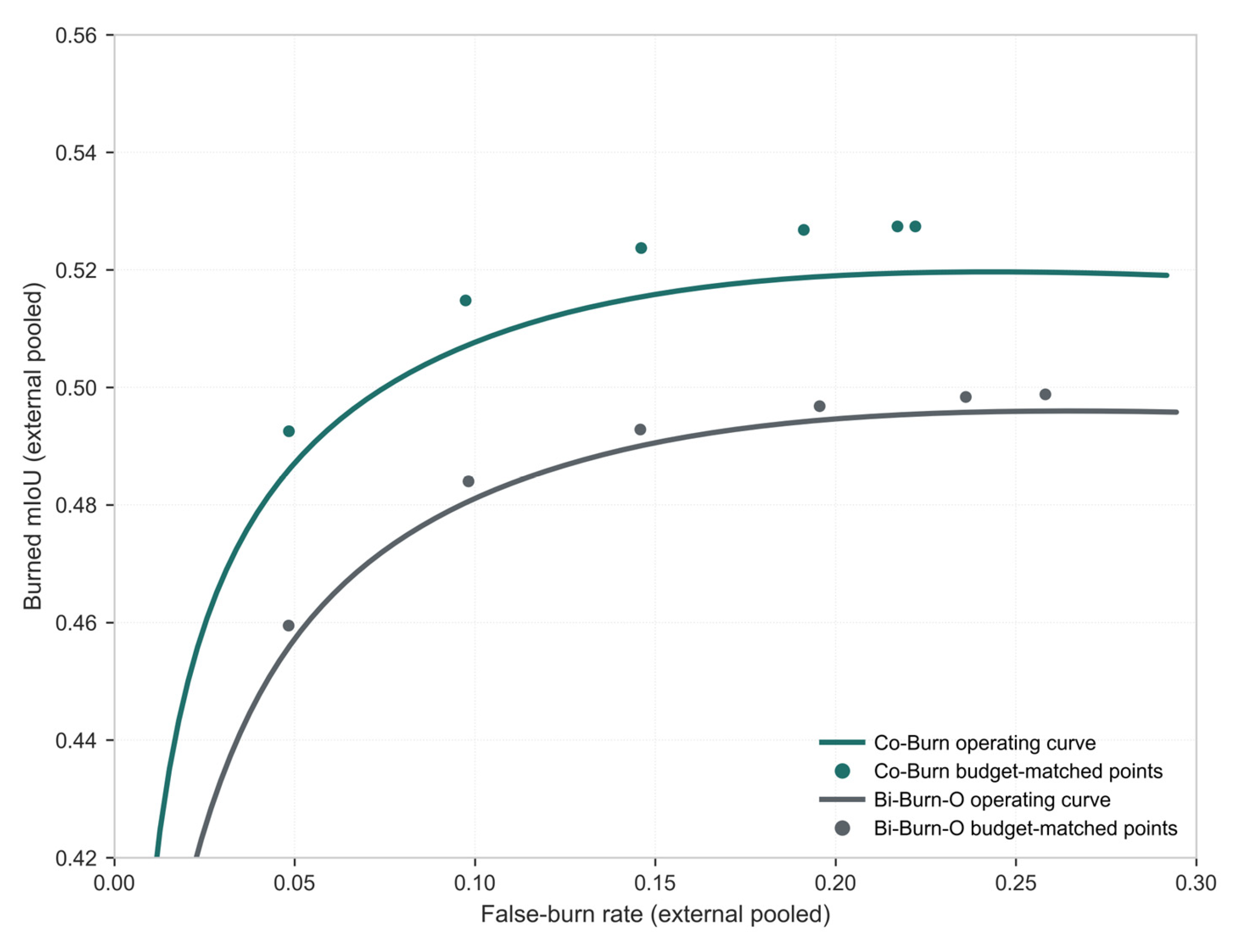
The nominal variants Bi-Burn and Bi-Burn-S were decoded by per-pixel argmax and did not use a burn gate under the adopted inference protocol. The main-benchmark predictions for Bi-Burn-O and Co-Burn use the fixed benchmark point ${\mathsf{\tau }}_{\mathrm{b}}={\mathsf{\tau }}_{\mathrm{h}}=0.5$. The same thresholds were applied across seeds and events and were not selected by optimising performance on the validation or external fires. The analysis below is retrospective: it uses the external references to sweep ${\mathsf{\tau }}_{\mathrm{b}}$ after training and compare the two conditional variants under common false-burn-rate caps. The sweep is reported separately as an operating analysis, while the fixed-point benchmark is reported in the main external comparison.

For these two variants, we varied ${\mathsf{\tau }}_{\mathrm{b}}$ from 0 to 1 in steps of 0.01 while holding ${\mathsf{\tau }}_{\mathrm{h}}=0.5$ and recorded the external pooled false-burn rate and burned mIoU for each seed at every threshold. We then compared them under common false-burn budgets. For each seed and each budget $\mathsf{\beta }\in \left\{0.05,0.10,\cdots ,0.30\right\}$, we selected the ${\mathsf{\tau }}_{\mathrm{b}}$ that gave the highest burned mIoU while keeping the pooled false-burn rate at or below $\mathsf{\beta }$, and we recorded that burned mIoU. The budget comparisons were matched within each seed before cross-seed aggregation and summarized as mean ± standard deviation.

3.6.4. Raw-dNBR Context of the Reference Class-1 and Class-2 Boundary

To characterise the raw-dNBR expression of the FESM reference boundary between classes 1 and 2, we analysed seven evaluation events, the validation events c, d, and h and the external events k, l, m, and n. For event $r$, raw dNBR was taken from the paired pre-fire and post-fire images before the clipping used for model input in Section 3.2.2. The analysis used only valid reference Class-1 and Class-2 pixels. For each event, a threshold ${\tau }_r$ was set by maximizing Youden’s J statistic for separating reference Class 2 from Class 1.

Let ${\mathsf{\Omega }}_{r,2}$ be the reference Class-2 pixels of event $r$. The high-dNBR concentration ratio (HCR) is

$${\mathrm{H}\mathrm{C}\mathrm{R}}_r={\displaystyle \frac{|\left\{i\in {\mathsf{\Omega }}_{r,2}:{\mathrm{d}\mathrm{N}\mathrm{B}\mathrm{R}}_{r,i}^{\mathrm{r}\mathrm{a}\mathrm{w}}\ge {\tau }_r\right\}|}{|{\mathsf{\Omega }}_{r,2}|}},$$

(19)

the share of reference Class-2 pixels on the high-dNBR side of ${\tau }_{\mathrm{r}}$. Separation of the two reference classes in raw dNBR is summarized by ${1-\mathrm{A}\mathrm{U}\mathrm{C}}_r$, where ${\mathrm{A}\mathrm{U}\mathrm{C}}_r$ is the area under the receiver operating characteristic (ROC) curve for distinguishing reference Class 2 from Class 1 using raw dNBR. Lower values indicate clearer separation between the two reference classes. These quantities are computed from the fixed event imagery and FESM reference classes, so they are independent of model seed and prediction. They give the event-specific spectral context for the residual error patterns reported in Section 4.4.

3.7. Metrics, Aggregation, and Statistical Reporting

Let $y_p$ and ${\widehat{\mathrm{y}}}_p$ denote the reference and predicted severity class at pixel $p\in \mathsf{\Omega }$, respectively. Let ${ N}_{\mathrm{c},\mathrm{c}\prime }=|\left\{p\in \mathsf{\Omega }:y_p=c,{\widehat{\mathrm{y}}}_p=\mathrm{c}\prime \right\}|$ denote the number of pixels with reference class $c$ and predicted class $\mathrm{c}\prime$, where $c, \mathrm{c}\prime \in \left\{0,1,2\right\}$. The class-wise intersection-over-union (IoU) is

$${\mathrm{I}\mathrm{O}\mathrm{U}}_{\mathrm{c}}\left(\mathsf{\Omega }\right)={\displaystyle \frac{{ N}_{\mathrm{c},\mathrm{c}}\left(\mathsf{\Omega }\right)}{{\displaystyle {\sum }_{\mathrm{c}\prime =0}^2}{ N}_{\mathrm{c},\mathrm{j}}\left(\mathsf{\Omega }\right)+{\displaystyle {\sum }_{\mathrm{c}\prime =0}^2}{ N}_{\mathrm{c}\prime ,\mathrm{c}}\left(\mathsf{\Omega }\right)-{ N}_{\mathrm{c},\mathrm{c}}\left(\mathsf{\Omega }\right)}}$$

(20)

and the burned mean IoU is

$${\mathrm{m}\mathrm{I}\mathrm{o}\mathrm{U}}_{\mathrm{b}\mathrm{u}\mathrm{r}\mathrm{n}\mathrm{e}\mathrm{d}}\left(\mathsf{\Omega }\right)={\displaystyle \frac{1}{2}}\left[{\mathrm{I}\mathrm{o}\mathrm{U}}_1\left(\mathsf{\Omega }\right)+{\mathrm{I}\mathrm{o}\mathrm{U}}_2\left(\mathsf{\Omega }\right)\right].$$

(21)

This metric gives equal weight to agreement for the low-to-moderate and high-severity classes. Class-specific IoU values were also reported. Overall quadratic weighted kappa (QWK) was calculated from the full three-class confusion matrix as a supplementary ordered-agreement metric. Quadratic weights were $w_{c,c\prime }={(c-c\prime )}^2/{\left(K-1\right)}^2$, with $K=3.$

False-burn rate is the proportion of reference Class-0 pixels assigned to either burned class,

$$\mathrm{F}\mathrm{B}\mathrm{R}\left(\mathsf{\Omega }\right)={\displaystyle \frac{{ N}_{0,1}\left(\mathsf{\Omega }\right)+{ N}_{0,2}\left(\mathsf{\Omega }\right)}{{\displaystyle {\sum }_{c\prime =0}^2}{ N}_{0,c\prime }\left(\mathsf{\Omega }\right)}}.$$

(22)

Let $\mathcal{R}$ denote the set of external events. For a fixed seed, pixel-pooled metrics were computed from confusion counts summed across the external events,

$$N_{\mathrm{c},\mathrm{c}\prime }^{pool}=\sum _{r\in \mathcal{R}}{ N}_{\mathrm{c},\mathrm{c}\prime }\left({\mathsf{\Omega }}_{\mathrm{r}}\right).$$

(23)

and metrics were then calculated from the pooled counts. Event-mean burned mIoU averaged the event-level values within seed,

$${\mathrm{m}\mathrm{I}\mathrm{o}\mathrm{U}}_{\mathrm{b}\mathrm{u}\mathrm{r}\mathrm{n}\mathrm{e}\mathrm{d}}^{\mathrm{e}\mathrm{v}\mathrm{e}\mathrm{n}\mathrm{t}-\mathrm{m}\mathrm{e}\mathrm{a}\mathrm{n}}={\displaystyle \frac{1}{\left|\mathcal{R}\right|}}\sum _{r\in \mathcal{R}}{\mathrm{m}\mathrm{I}\mathrm{o}\mathrm{U}}_{\mathrm{b}\mathrm{u}\mathrm{r}\mathrm{n}\mathrm{e}\mathrm{d}}\left({\mathsf{\Omega }}_{\mathrm{r}}\right)$$

(24)

where ${\mathsf{\Omega }}_{\mathrm{r}}$ denotes the valid pixels of event $r$. The relative validation-to-external gap in burned mIoU was obtained using

$${\mathrm{G}\mathrm{a}\mathrm{p}}_{\mathrm{r}\mathrm{e}\mathrm{l}}\left(\%\right)=100\times {\displaystyle \frac{{\mathrm{m}\mathrm{I}\mathrm{o}\mathrm{U}}_{\mathrm{b}\mathrm{u}\mathrm{r}\mathrm{n}\mathrm{e}\mathrm{d}}^{\mathrm{v}\mathrm{a}\mathrm{l}}-{\mathrm{m}\mathrm{I}\mathrm{o}\mathrm{U}}_{\mathrm{b}\mathrm{u}\mathrm{r}\mathrm{n}\mathrm{e}\mathrm{d}}^{\mathrm{e}\mathrm{x}\mathrm{t},\mathrm{p}\mathrm{o}\mathrm{o}\mathrm{l}}}{{\mathrm{m}\mathrm{I}\mathrm{o}\mathrm{U}}_{\mathrm{b}\mathrm{u}\mathrm{r}\mathrm{n}\mathrm{e}\mathrm{d}}^{\mathrm{v}\mathrm{a}\mathrm{l}}}}.$$

(25)

${\mathrm{G}\mathrm{a}\mathrm{p}}_{\mathrm{r}\mathrm{e}\mathrm{l}}$ was reported as a descriptive transfer summary, with lower values indicating less relative loss from validation to external events. Here, ${\mathrm{m}\mathrm{I}\mathrm{o}\mathrm{U}}_{\mathrm{b}\mathrm{u}\mathrm{r}\mathrm{n}\mathrm{e}\mathrm{d}}^{\mathrm{v}\mathrm{a}\mathrm{l}}$ is obtained by the same pixel-pooled aggregation as Equation (23), applied to validation scenes c, d, and h. ${\mathrm{m}\mathrm{I}\mathrm{o}\mathrm{U}}_{\mathrm{b}\mathrm{u}\mathrm{r}\mathrm{n}\mathrm{e}\mathrm{d}}^{\mathrm{e}\mathrm{x}\mathrm{t},\mathrm{p}\mathrm{o}\mathrm{o}\mathrm{l}}$ is calculated from the pooled external confusion counts.

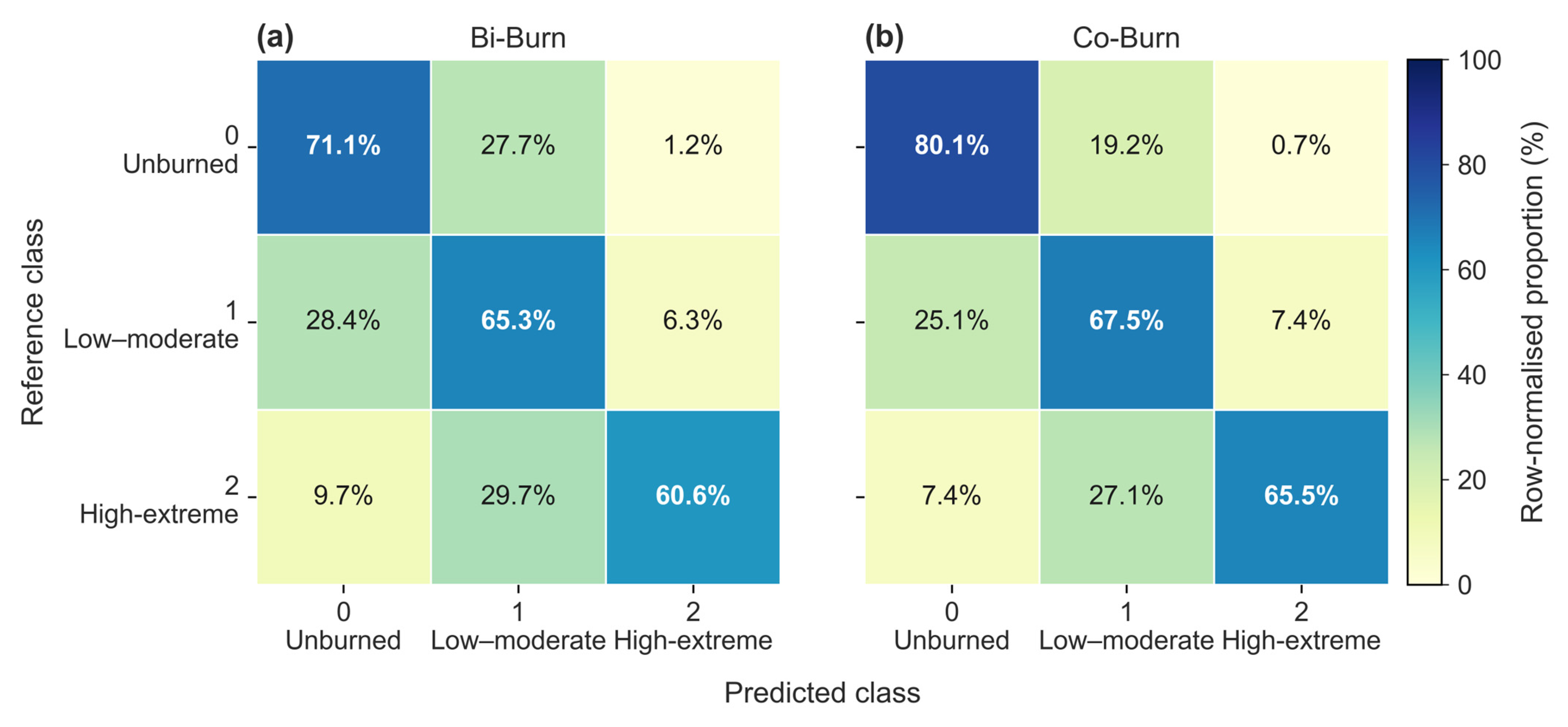
Scalar metrics for trainable models were summarized as mean ± standard deviation across the five runs. For pooled confusion-matrix displays, event-level counts were first summed across the four external fires within each seed, normalised by reference-class row, and then averaged elementwise across seeds. Event-level diagnostic matrices were constructed separately for each fire using the same row normalization and cross-seed averaging. These matrices distinguish false-burn expansion from upward and downward transitions between severity classes.

4. Results

4.1. Cross-Event Benchmark Under Pooled and Event-Mean Aggregation

Across the four held-out external events, Co-Burn achieved the highest burned mIoU among the ten evaluated methods under both aggregation rules, reaching 0.520 ± 0.017 for pixel-pooled evaluation and 0.524 ± 0.028 for event-mean evaluation (

Table 4. External benchmark across the ten evaluated methods, with validation performance for reference. External metrics are calculated on the four held-out external fires. Values for learned models are mean ± standard deviation across five training seeds. The dNBR threshold baseline is deterministic. Bold marks the best value in each column.

Model	Input	Output	Validation Burned mIoU	External Burned mIoU (Pooled)	External Burned mIoU (Event-Mean)	External Class-2 IoU	Overall QWK	${\mathbf{G}\mathbf{a}\mathbf{p}}_{\mathbf{r}\mathbf{e}\mathbf{l}}$ (%)
dNBR threshold	dNBR only	Fixed thresholds	0.564	0.380	0.331	0.503	0.640	32.6
DeepLabv3+	bi-temporal, early fusion	Nominal multiclass	0.656 ± 0.097	0.378 ± 0.037	0.419 ± 0.042	0.479 ± 0.031	0.623 ± 0.056	41.7 ± 6.0
Siamese U-Net	bi-temporal	Nominal multiclass	0.732 ± 0.015	0.447 ± 0.035	0.475 ± 0.051	0.522 ± 0.027	0.690 ± 0.023	38.9 ± 3.7
SNUNet -CD	bi-temporal	Nominal multiclass	0.653 ± 0.021	0.468 ± 0.010	0.453 ± 0.009	0.551 ± 0.019	0.628 ± 0.050	28.3 ± 3.1
BIT	bi-temporal	Nominal multiclass	0.665 ± 0.018	0.474 ± 0.015	0.475 ± 0.027	0.551 ± 0.006	0.672 ± 0.030	28.7 ± 1.6
BiRAUnet-NBR	bi-temporal + dNBR-family indices	Nominal multiclass	0.749 ± 0.004	0.416 ± 0.015	0.445 ± 0.016	0.495 ± 0.016	0.661 ± 0.014	44.5 ± 2.0
Bi-Burn	bi-temporal	Nominal multiclass	0.647 ± 0.031	0.474 ± 0.018	0.453 ± 0.015	0.563 ± 0.025	0.654 ± 0.023	26.6 ± 5.2
Bi-Burn-S	bi-temporal + dNBR	Nominal multiclass	0.684 ± 0.007	0.492 ± 0.008	0.514 ± 0.014	0.581 ± 0.010	0.710 ± 0.007	28.0 ± 1.2
Bi-Burn-O	bi-temporal	Conditional ordinal	0.645 ± 0.026	0.491 ± 0.018	0.468 ± 0.016	0.596 ± 0.024	0.657 ± 0.042	23.7 ± 4.4
Co-Burn	bi-temporal + dNBR	Conditional ordinal	0.659 ± 0.028	0.520 ± 0.017	0.524 ± 0.028	0.607 ± 0.018	0.728 ± 0.023	20.9 ± 5.1

). It also recorded the smallest relative validation-to-external gap, 20.9 ± 5.1%, and the highest overall QWK, 0.728 ± 0.023. At the event level, no method led on all four fires. Co-Burn ranked first on Nerriga and Grafton and Bi-Burn-S led Talbingo and Pilliga West (

Table A1. Per-event burned mIoU on the four held-out external fire events. Percentages in parentheses show each event’s share of the valid external pixels used for pixel-pooled evaluation. Learned-model values are five-seed means; the dNBR threshold baseline is deterministic. Event mean weights the four fires equally, whereas pixel-pooled burned mIoU is computed from pooled external confusion counts. Bold marks the highest value in each column.

Model	k Nerriga (14.7%)	l Talbingo (40.6%)	m Grafton (36.0%)	n Pilliga West (8.7%)	Event Mean	Pixel Pooled
dNBR threshold	0.485	0.510	0.134	0.196	0.331	0.380
DeepLabv3+	0.464	0.484	0.078	0.652	0.419 ± 0.042	0.378 ± 0.037
Siamese U-Net	0.585	0.538	0.149	0.628	0.475 ± 0.051	0.447 ± 0.035
SNUNet-CD	0.598	0.537	0.205	0.472	0.453 ± 0.009	0.468 ± 0.010
BIT	0.592	0.581	0.184	0.544	0.475 ± 0.027	0.474 ± 0.015
BiRAUnet-NBR	0.463	0.544	0.111	0.660	0.445 ± 0.016	0.416 ± 0.015
Bi-Burn	0.631	0.565	0.182	0.435	0.453 ± 0.015	0.474 ± 0.018
Bi-Burn-S	0.597	0.625	0.153	0.680	0.514 ± 0.014	0.492 ± 0.008
Bi-Burn-O	0.664	0.578	0.197	0.434	0.468 ± 0.016	0.491 ± 0.018
Co-Burn	0.665	0.618	0.216	0.596	0.524 ± 0.028	0.520 ± 0.017

). Excluding Pilliga West left Co-Burn first under both aggregation rules, although the remaining order changed (Appendix A.5).

BiRAUnet-NBR led the validation ranking at 0.749 ± 0.004, but that lead did not carry to the external fires. Its external pixel-pooled burned mIoU was 0.416 ± 0.015, giving the largest relative validation-to-external gap in the benchmark at 44.5 ± 2.0%.

Figure 3 visualizes the rank changes produced by reweighting the four external fires from valid-pixel support to equal event weight.

The class-specific results in

Table A2. External class-specific IoU for the two burned severity classes across the four held-out fires. Values are pixel-pooled IoUs computed by summing confusion matrices across events k, l, m, and n. Learned models are reported as mean ± standard deviation across five seeds. The fixed dNBR threshold baseline has no seed variation. The average of Class-1 and Class-2 IoU equals the pixel-pooled burned mIoU in Table 4 up to rounding. Bold marks the highest value in each column.

Model	Class-1 IoU	Class-2 IoU
dNBR threshold	0.256	0.503
DeepLabv3+	0.278 ± 0.091	0.479 ± 0.031
Siamese U-Net	0.373 ± 0.044	0.522 ± 0.027
SNUNet-CD	0.384 ± 0.017	0.551 ± 0.019
BIT	0.397 ± 0.030	0.551 ± 0.006
BiRAUnet-NBR	0.336 ± 0.021	0.495 ± 0.016
Bi-Burn	0.386 ± 0.016	0.563 ± 0.025
Bi-Burn-S	0.403 ± 0.013	0.581 ± 0.010
Bi-Burn-O	0.387 ± 0.019	0.596 ± 0.024
Co-Burn	0.434 ± 0.022	0.607 ± 0.018

show that Co-Burn still ranked first for both classes, reaching a Class-1 IoU of 0.434 ± 0.022 and a Class-2 IoU of 0.607 ± 0.018. For every evaluated method, Class-1 IoU was lower than Class-2 IoU, making low-to-moderate severity the more difficult burned class.

Figure 4 shows a fixed region of interest (ROI) from external event m, Grafton. The FESM-derived target contains a compact Class-2 core, a surrounding Class-1 zone, and an unburned strip along the south-western edge. Errors in this ROI mainly involve fragmentation of the Class-2 core and displacement of the Class-0/Class-1 boundary. Co-Burn retains the south-western unburned strip while preserving the Class-2 core and the intervening Class-1 zone within this local ROI.

4.2. Matched Factorial Analysis of dNBR Anchoring and Conditional Ordinal Formulation

Table 5. Factorial comparison of dNBR anchoring and the conditional ordinal formulation. Panel A reports external burned mIoU and false-burn rate for the four matched variants as mean ± SD across five training runs. Panel B reports event-level factorial contrasts for each external fire, with equal-event mean and leave-one-fire-out mean range.

(A). Four factorial cells.
Variant	dNBR Anchoring	Conditional Ordinal Formulation		External Burned mIoU		False-Burn Rate
Bi-Burn	No	No		0.474 ± 0.018		0.289 ± 0.113
Bi-Burn-S	Yes	No		0.492 ± 0.008		0.062 ± 0.033
Bi-Burn-O	No	Yes		0.491 ± 0.018		0.329 ± 0.207
Co-Burn	Yes	Yes		0.520 ± 0.017		0.199 ± 0.096
(B). Event-level factorial contrasts.
Outcome	Factorial Term	Nerriga	Talbingo	Grafton	Pilliga West	Equal-Event Mean	LOO Mean Range
Burned mIoU	dNBR anchoring	−0.0171	0.0503	−0.0048	0.2032	0.0579	0.0095 to 0.0829
Burned mIoU	Conditional ordinal formulation	0.0504	0.0034	0.0389	−0.0428	0.0125	−0.0002 to 0.0309
Burned mIoU	Interaction	0.0345	−0.0196	0.0471	−0.0829	−0.0052	−0.0227 to 0.0207
FBR	dNBR anchoring	−0.1928	−0.1972	−0.0756	−0.4470	−0.2281	−0.2790 to −0.1552
FBR	Conditional ordinal formulation	0.1300	0.0924	0.1077	−0.0006	0.0824	0.0665 to 0.1100
FBR	Interaction	0.1933	0.0835	0.0760	0.1836	0.1341	0.1144 to 0.1535

separates the performance of the four matched variants from the event-level factorial contrasts.

The burned-mIoU contrasts varied among the four external fires. The dNBR effect ranged from −0.017 on Nerriga to +0.203 on Pilliga West, with an equal-event mean of +0.058. The conditional ordinal effect was positive on Nerriga, Talbingo, and Grafton and negative on Pilliga West, giving an equal-event mean of +0.012. The interaction changed sign among fires and had an equal-event mean of −0.005. The corresponding pixel-pooled descriptive effects were +0.024 for dNBR anchoring and +0.023 for the conditional ordinal formulation. Pixel pooling weights fires according to their valid-pixel support, while the event-level summary gives each fire equal weight.

False-burn rate showed a clearer directional pattern for the dNBR axis. The dNBR contrast was negative on all four external fires, ranging from −0.076 on Grafton to −0.447 on Pilliga West, with an equal-event mean of −0.228. The conditional ordinal and interaction contrasts had equal-event means of +0.082 and +0.134, respectively. The positive interaction indicates that the reduction in false-burn rate associated with dNBR was smaller under the conditional ordinal formulation than under the nominal formulation.

Figure 5 shows how these differences appear in the full-configuration error structure. The share of reference-unburned pixels assigned to burned classes decreased from 28.9% for Bi-Burn to 19.9% for Co-Burn. The reduction consisted mainly of fewer Class-0-to-Class-1 predictions, which fell from 27.7% to 19.2%, while Class-0-to-Class-2 predictions changed from 1.2% to 0.7%. Omission from the reference-burned classes also decreased. Class-1-to-Class-0 errors fell from 28.4% to 25.1%, and Class-2-to-Class-0 errors fell from 9.7% to 7.4%.

4.3. Operating Trade-Off Between False-Burn Rate and Burned mIoU

The conditional variants decode at the fixed benchmark point ${\mathsf{\tau }}_{\mathrm{b}}={\mathsf{\tau }}_{\mathrm{h}}=0.5$. Sweeping ${\mathsf{\tau }}_{\mathrm{b}}$ traces the trade-off as specified in Section 3.6.3. Figure 6 shows the resulting operating curves for Bi-Burn-O and Co-Burn. Bi-Burn-O and Co-Burn share the conditional ordinal formulation, so this comparison isolates the dNBR-anchored input design within that formulation.

We then compared their burned mIoU under common pooled false-burn-rate caps from 0.05 to 0.30. All six budgets were available for both variants across the five seeds. Co-Burn reached a higher burned mIoU than Bi-Burn-O in all 30 seed-budget comparisons, with mean paired gains from +0.029 to +0.033. At a budget of 0.20, Co-Burn reached 0.527 ± 0.022, compared with 0.497 ± 0.022 for Bi-Burn-O. At the two loosest caps, the selected Co-Burn operating points also had lower mean achieved false-burn rates while retaining higher burned mIoU (

Table A3. Budget-constrained external operating points under common false-burn-rate caps. ${∆\mathrm{m}\mathrm{I}\mathrm{o}\mathrm{U}}_{\mathrm{b}\mathrm{u}\mathrm{r}\mathrm{n}\mathrm{e}\mathrm{d}}$ is calculated as Co-Burn minus Bi-Burn-O under the same false-burn-rate cap. FBR denotes the achieved pooled false-burn rate.

Common FBR Cap $\mathsf{\beta }$	Bi-Burn-O Burned mIoU ${\mathbf{m}\mathbf{I}\mathbf{o}\mathbf{U}}_{\mathbf{b}\mathbf{u}\mathbf{r}\mathbf{n}\mathbf{e}\mathbf{d}}$	Co-Burn Burned mIoU ${\mathbf{m}\mathbf{I}\mathbf{o}\mathbf{U}}_{\mathbf{b}\mathbf{u}\mathbf{r}\mathbf{n}\mathbf{e}\mathbf{d}}$	Paired Burned mIoU ${∆\mathbf{m}\mathbf{I}\mathbf{o}\mathbf{U}}_{\mathbf{b}\mathbf{u}\mathbf{r}\mathbf{n}\mathbf{e}\mathbf{d}}$	Seeds with Co-Burn > Bi-Burn-O	Bi-Burn-O Achieved FBR	Co-Burn Achieved FBR
0.05	0.460 ± 0.020	0.493 ± 0.020	+0.033 ± 0.018	5/5	0.0483 ± 0.0008	0.0483 ± 0.0006
0.10	0.484 ± 0.022	0.515 ± 0.022	+0.031 ± 0.020	5/5	0.0982 ± 0.0004	0.0974 ± 0.0012
0.15	0.493 ± 0.022	0.524 ± 0.023	+0.031 ± 0.021	5/5	0.1458 ± 0.0017	0.1461 ± 0.0017
0.20	0.497 ± 0.022	0.527 ± 0.022	+0.030 ± 0.021	5/5	0.1956 ± 0.0024	0.1912 ± 0.0029
0.25	0.498 ± 0.022	0.527 ± 0.022	+0.029 ± 0.022	5/5	0.2360 ± 0.0210	0.2171 ± 0.0241
0.30	0.499 ± 0.022	0.527 ± 0.022	+0.029 ± 0.022	5/5	0.2581 ± 0.0369	0.2221 ± 0.0303

).

Figure 7 places this comparison in a fixed external ROI near a reference class-0 boundary. At a 0.20 false-burn-rate budget, Co-Burn keeps a continuous reference-unburned region that Bi-Burn-O draws into the burned map, while preserving the surrounding Class-1 zone and the Class-2 core. The comparison panel marks reference-unburned pixels that Bi-Burn-O assigns to Class 1 and Co-Burn keeps as Class 0.

4.4. Event-Level Downward Shift in Grafton

Grafton was the lowest-scoring external fire for every evaluated method (Table A1). On this fire, Co-Burn kept 82.4% of reference Class-0 pixels unburned, so false-burn expansion stayed limited. The errors instead ran downward among reference-burned pixels: 61.3% of Class-2 pixels were graded Class 1 and 28.3% Class 0, and 43.8% of Class-1 pixels fell to Class 0. Grafton’s low burned mIoU thus came from downward movement through the ordered classes.

Figure 8e shows that this movement was spatially coherent. Class-1-to-Class-0 errors covered broad areas across the mapped burned support, while Class-2-to-Class-1 and Class-2-to-Class-0 errors clustered within the high-severity reference areas.

In the displayed Grafton ROI, raw dNBR changes gradually across the reference Class-1/Class-2 boundary. Across the seven evaluation events, Grafton showed the weakest raw-dNBR separation between these classes, with $\mathrm{H}\mathrm{C}\mathrm{R}=0.418$ and $1-\mathrm{A}\mathrm{U}\mathrm{C}=0.409$ (Table A4).

5. Discussion

5.1. Anchoring Burned-Footprint Placement and Organizing Severity Grades

The four matched Bi-Burn variants hold the backbone, training schedule, evaluation protocol, and burn-presence supervision fixed. Within this design, the input axis adds dNBR, and the output axis replaces the nominal severity formulation with the conditional ordinal formulation. The event-level effects varied among the four external fires, while their false-burn and class-level patterns showed clearer directional differences. In particular, dNBR anchoring reduced false-burn rate on all four external fires.

The dNBR channel reorganises the B8 and B12 measurements already present at both dates into an explicit pixel-aligned pre-to-post contrast that enters the post-fire encoder before the two temporal streams meet at the bottleneck. The fixed-threshold baseline separates unburned from burned pixels at 0.10 and the two burned grades at 0.44. Both decisions are therefore tied to the same dNBR axis. When the dNBR distribution shifts between fires, the two cuts remain fixed, but the proportions of pixels falling on either side can change. The mapped burned extent and severity composition may both change as a result.

The conditional formulation separates burn presence from high-severity assignment. It predicts $p_b$ for burn presence and $p_h$ for high severity within burned pixels. The nominal arm receives the same burn-presence supervision during training but obtains its final class map from the three-class softmax. For the conditional variants, varying the burn-presence threshold ${\tau }_b$ changes which pixels enter the burned footprint while the high-severity threshold ${\tau }_h$ remains fixed. This is how the false-burn-rate operating analysis in Section 4.3 varies footprint entry. The nominal models were decoded by argmax and did not use the burn gate under the adopted inference protocol.

With reflectance-only input, replacing the nominal formulation with the conditional ordinal formulation increased Class-2 IoU from 0.563 to 0.596, while Class-1 IoU changed from 0.386 to 0.387. Under the conditional formulation, adding dNBR increased Class-1 IoU from 0.387 to 0.434 and Class-2 IoU from 0.596 to 0.607.

False-burn errors were concentrated in Class 1. Of Bi-Burn’s 28.9 false-burn percentage points, 27.7 came from Class-0-to-Class-1 errors. For Co-Burn, the corresponding values were 19.2 of 19.9 percentage points. The reduction from Bi-Burn to Co-Burn therefore removed a substantial source of Class-1 false positives. Co-Burn ranked first for both burned classes, while Class 1 remained the more difficult burned category across the evaluated methods.

Class 1 receives errors from both neighbouring classes. Outward footprint expansion moves reference Class-0 pixels into Class 1, and downward severity assignment moves Class-2 pixels into Class 1. Reference Class-1 pixels are also reassigned to Class 0 or Class 2. In addition, Class 1 combines low and moderate severity, and moderate severity had the lowest class-specific accuracy in the original FESM assessment.

5.2. What Burned mIoU Hides at the Event Level

Burned mIoU gives the same penalty to errors that expand the map, omit burned pixels, or change the burned grade, although they leave the map wrong in different ways. False-burn rate isolates outward expansion, but no corresponding scalar is reported here for omission, so the confusion matrix is needed to show whether burned pixels left the footprint or changed grade. The pooled external matrix shows that Co-Burn reduced omission as well as false expansion relative to Bi-Burn.

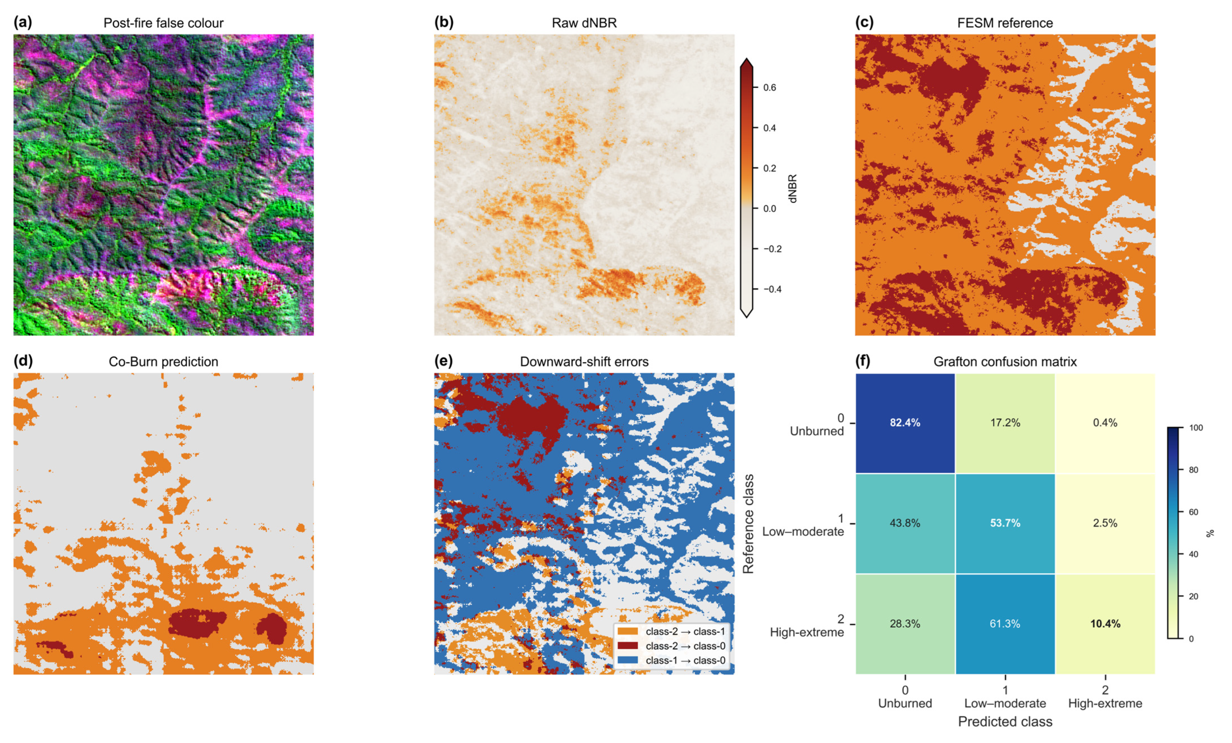
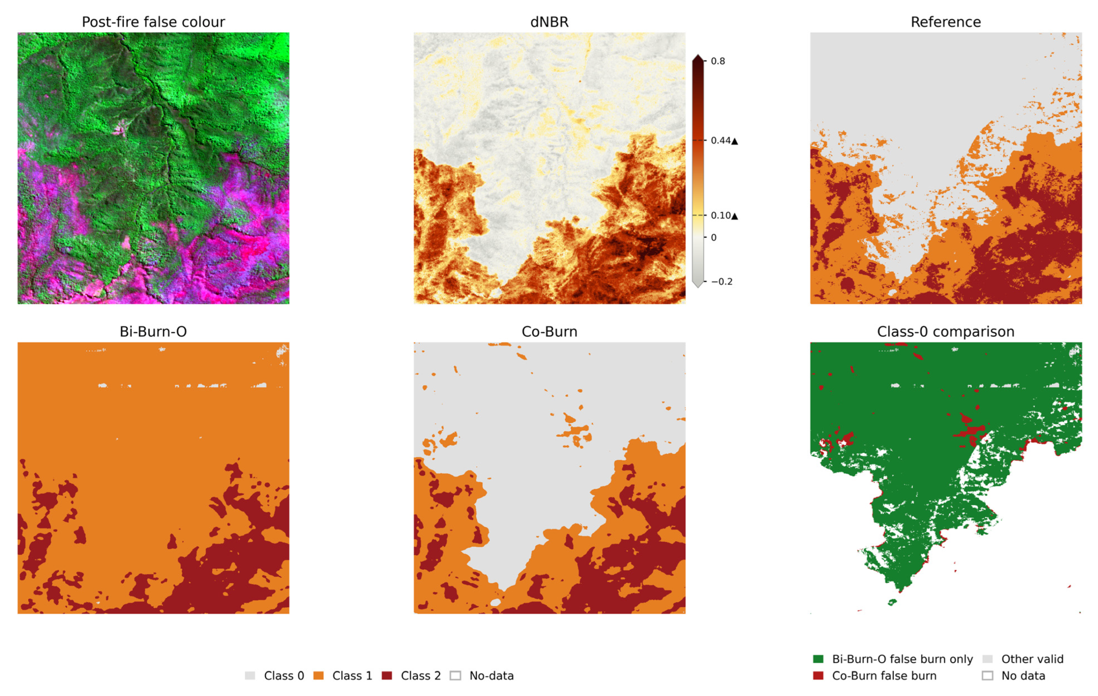
Grafton had a different error profile from the pooled external result. It was the hardest external fire for every method, with Co-Burn still recording the highest event score at 0.216. Co-Burn retained 82.4% of reference Class-0 pixels, slightly above its pooled value of 80.1%, while the reference-burned rows showed severe omission and downward reassignment. Only 10.4% of reference Class-2 pixels remained in Class 2, compared with 65.5% in the pooled matrix. The remaining errors shifted downward into Class 1 or Class 0, alongside substantial Class-1-to-Class-0 omission reported in Section 4.4.

These downward movements had different consequences for the map. A Class-2 pixel shifted to Class 1 remained inside the burned footprint but was reported at a lower severity, whereas a transition from either burned class to Class 0 removed the pixel from the mapped footprint altogether. Figure 8e shows that these errors were also distributed differently across the fire. Class-1-to-Class-0 losses extended over broad burned areas, while Class-2 errors were concentrated within the high-severity reference cores.

Raw dNBR was also least informative at Grafton’s upper severity boundary. It showed the weakest Class-1/Class-2 separation among the seven evaluation events, and most reference Class-2 pixels remained on the low-dNBR side even at the event-specific cut (Table A4). This weak spectral separation occurred at the same boundary where downward severity errors were concentrated. Grafton’s difficulty was concentrated in the reference-burned classes, with broad Class-1 omission, strong downward reassignment from Class 2, and the weakest raw-dNBR separation at the Class-1/Class-2 boundary. All ten methods reached their lowest event-level burned mIoU on this fire, while Co-Burn remained the highest-scoring method at 0.216.

5.3. Complete-Event Evaluation of Cross-Event Transfer

The validation and external sets both contain complete held-out fires, but they serve different roles. Validation burned mIoU selected the retained checkpoint for every trainable model. No external fire contributed to model fitting, configuration selection, checkpoint selection, or the fixed operating rules. The two sets therefore separate development-stage selection from evaluation on untouched events.

BiRAUnet-NBR ranked first on validation, whereas Co-Burn ranked first on the four external fires. BiRAUnet-NBR had the largest relative validation-to-external decline in the benchmark, at 44.5%, and Co-Burn the smallest, at 20.9%. Siamese U-Net also ranked near the top on validation but was among the three methods with the largest external declines. The four Bi-Burn variants occupied the four smallest gaps, from 20.9% to 28.0%.

Talbingo and Grafton supplied 76.6% of the valid external pixels and carried most of the weight in the pixel-pooled result. Event-mean aggregation counted each fire once, moving Siamese U-Net from seventh under pixel pooling to joint third under event averaging. Co-Burn ranked first under both aggregation rules, and excluding Pilliga West did not change that result.

5.4. Scope and Applicability

Co-Burn is designed for post-fire severity mapping of previously unseen forest fire events when pre-fire and post-fire Sentinel-2 imagery is available but reference labels for the target event are not. Because deployment does not require target-event labels, the method can support post-fire recovery prioritisation, rapid early post-fire assessment, and repeated severity mapping across successive fires without event-specific relabelling. When combined with the additional information required for these applications, the resulting severity maps can also provide an input to longer-term assessments of ecological impacts and carbon loss. Such mapping has practical value because high-severity areas, extensive burning, and repeated fires are major drivers of biodiversity loss in Australian megafires [43].

The evidence reported here quantifies agreement with the three-class FESM reference across fourteen forest fires in New South Wales. Evaluation is confined to the valid FESM extent of each event. Pixels outside this reference extent were excluded, so the reported metrics describe complete-event performance within the valid FESM extent. FESM is an operational remote-sensing product derived from Sentinel-2 imagery and supervised classification [7], rather than an independent field measurement of ecological severity. dNBR is one of several spectral-change and vegetation predictors used in FESM, so agreement with the FESM-derived labels does not provide an independent validation of the dNBR anchoring mechanism. Reference uncertainty is also relevant near adjacent severity boundaries. Moderate severity had the lowest class-specific accuracy in the original Sentinel-2 FESM assessment, and disagreements between Sentinel-2 and Landsat FESM products commonly occurred between adjacent severity classes [40]. Independent field observations remain necessary to establish how the mapped classes correspond to ecological severity on the ground.

The demonstrated transfer is bounded by the vegetation and observation conditions represented in the current dataset. The fourteen events represent forest environments in New South Wales and do not test transfer to tropical rainforest, boreal coniferous forest, grassland, or savanna fire regimes. The three classes describe canopy response, and previous studies have shown that the correspondence between spectral indices and severity can vary with vegetation type and environmental conditions [19,20]. Evaluation in other biomes therefore requires reference labels appropriate to their vegetation structure and severity definitions. Observation conditions also delimit the demonstrated transfer. The four external fires were represented by event-specific acquisition and compositing windows, so the cross-event benchmark includes variation in image timing and compositing conditions alongside differences in fire and vegetation conditions. These acquisition conditions were not separated experimentally across the external test set.

HCR and 1 − AUC depend on the reference classes of the target fire and therefore serve as retrospective diagnostics. Deployment-time screening requires label-free information available at inference, such as the proportion of usable pixels retained after cloud and quality screening or disagreement among independently trained models. Prospective evaluation on newly observed fires should use independent field severity measurements as reference, with the burn gate calibrated on development fires and fixed before deployment. This would test whether the fixed operating rule transfers to new fire events while extending evaluation across additional vegetation types, fire regimes, geographic regions, and acquisition conditions. Such evaluation could also assess whether additional spectral features and complementary sensors improve separability at the Class-1/Class-2 boundary, which remained the least separable part of the current target.

6. Conclusions

Cross-event burn-severity mapping can be formulated as two linked decisions: locating the burned footprint and grading severity within the burned area. Co-Burn organises these decisions within a single bi-temporal Siamese model. A dNBR anchor on the post-fire branch provides an explicit representation of pre-to-post spectral change, while a conditional ordinal head first estimates burn presence and then assigns high severity within burned pixels. The contributions of this study are threefold.

First, Co-Burn structurally separates burned-footprint placement from within-footprint severity grading within a shared pixel-wise network. The conditional ordinal head treats burn presence as the first decision and evaluates high severity conditional on that decision, allowing the ordered relationship among the classes to enter the output formulation directly rather than relying solely on competition among three nominal softmax classes.

Second, the matched $2\times 2$ design evaluates input anchoring and output formulation as controlled experimental factors. With the backbone, training protocol, and burn-presence supervision held common, the burned-mIoU effects of the two design axes varied among fire events, while dNBR anchoring reduced false-burn rate on all four external fires. The dNBR-anchored variants also showed lower run-to-run variation in false-burn rate across the five training runs. This controlled comparison allows the effects of input anchoring and output formulation to be examined separately under matched conditions, rather than collapsing both changes into a single overall performance gain.

Third, this study evaluates transfer to fire events kept entirely outside model development. Across ten methods and four external fires, Co-Burn achieved the highest external burned mIoU under both pixel-pooled and event-mean aggregation and had the smallest validation-to-external gap. The validation ranking did not identify the model that transferred best to the external fires. Complete-event evaluation also revealed error directions that are hidden by a single aggregate score. On the most difficult external fire, the low score mainly reflected underestimated severity and missed burned ground, not overestimation of burned area. A low aggregate score can therefore represent different mapping biases. Cross-event evaluation should report event-level error directions alongside pixel-pooled and event-mean summaries so that map users can determine whether a result is more likely to overestimate affected area, omit burned ground, or compress the severity distribution.