Automatic Identification and Assessment of Potential Geohazards in a Wide Area Based on Multisource Remote Sensing and Deep Learning

Highlights

What are the main findings?

• A novel automatic identification and quantitative assessment method for PGHs is proposed, improving the efficiency and accuracy of PGH spatial recognition.
• The overall spatial distribution characteristics of PGHs in the HBP region of Shanxi Province on the Loess Plateau are systematically clarified, and regional PGH risk levels are quantitatively graded.

What are the implications of the main findings?

• This provides a targeted technical framework for regional PGH investigation, dynamic monitoring, and risk assessment.
• This offers reliable data support and decision reference for ecological protection, geological risk prevention, and regional sustainable development in the Loess Plateau HBP region.

Abstract

Wide-area monitoring and accurate assessment of potential geohazards (PGHs) based on remote sensing will provide a crucial foundation for geohazard prevention and mitigation. Current remote sensing methods for PGH identification and evaluation require extensive manual effort and lack intelligence throughout the process. To effectively integrate multisource remote sensing data, we propose an automated method for identifying and assessing PGHs across a wide area. This approach integrates InSAR deformation, high-resolution optical remote sensing, terrain, and vector data of ground features to enable automated delineation of unstable zones, automatic identification of potentially threatened objects (PTOs), automatic screening of PGHs, and risk assessment. The proposed method is tested in the Hequ–Baode–Pianguan (HBP) region of Shanxi province. Using the DS-InSAR technique, we process 94 Sentinel-1 SAR images covering the HBP region from 2020 to 2024 to estimate surface stability. We automatically detect the boundaries of 161 active deformation areas (ADAs) in HBP. A deep learning model based on DeepLabV3+ processes optical remote sensing images of the study area at 0.5 m resolution to automatically identify all PTOs. By integrating terrain data and spatial relationships among PTOs and ADAs, we develop an algorithmic model to identify 90 PGHs and classify them into external-threat, internal-threat, and internal-external-threat geohazard zones. Finally, a risk matrix is created for an automatic geohazard risk assessment, producing results for all PGHs in the study area. This developed method will support wide-area screening and prioritization of potential geohazards on the Loess Plateau and improve PGH investigation capabilities.

1. Introduction

Geohazards, including uneven ground subsidence and landslides, are widespread and seriously threaten human life, property, and the ecological environment [1]. Remote sensing technologies for Earth observation, such as microwave and optical remote sensing, offer unique advantages for monitoring and identifying potential geohazards (PGHs) through non-contact, large-scale measurements and high efficiency. Wide-area-scale intelligent monitoring and risk assessment of PGHs based on multisource remote sensing data are of great significance for the prevention, control, and early warning of geohazards.

Interferometric Synthetic Aperture Radar (InSAR) enables millimeter-level measurement of surface deformation, with advantages including all-weather, all-time, low-cost, and regional applicability. It is widely applied to monitoring earthquakes, volcanoes, landslides, ground subsidence, and urban infrastructure safety [2,3,4,5]. In PGH monitoring, Qu et al. [6] used multisource SAR data and time-series InSAR to reveal the spatiotemporal evolution of ground subsidence in Xi’an, China, from 2005 to 2012, and demonstrated a correlation between subsidence and groundwater extraction. Dong et al. [7] monitored the precursory movement of the Xinmo landslide in Mao County, China, and identified a distinct seasonal displacement pattern in the landslide source area with rapid acceleration before failure, demonstrating the potential of InSAR for early landslide warning. Dong et al. [8] integrated the Small Baseline Subset InSAR (SBAS-InSAR) with a gradient boosting decision tree model and multisource environmental factors, including digital elevation model (DEM), slope, topographic wetness index (TWI), and normalized difference vegetation index (NDVI), to generate landslide susceptibility maps (LSMs). They also combined the Pearson correlation coefficient between InSAR time-series deformation and monthly rainfall to screen for active landslides, significantly improving the accuracy of landslide monitoring. Liu et al. [9] proposed an unsupervised method for automatic landslide extraction from InSAR deformation data using edge-threshold segmentation, adaptive histogram equalization, and morphological optimization. Yao et al. [10] analyzed the spatiotemporal evolution of reservoir-area landslides using multi-temporal InSAR (MT-InSAR) and introduced a seasonal fluctuation amplitude index to quantify rainfall and water-level effects. For the risk assessment of slow-moving landslides, Dai et al. [11] developed a cyclic assessment framework that integrates InSAR-derived deformation with geological factors, including lithology, slope, faults, and rainfall. Tian et al. [12] combined MT-InSAR with a Random Forest model and dynamic weighting to identify active landslides and assess rainfall-driven sensitivity in the Three Gorges Reservoir area. Zhu et al. [13] improved landslide identification accuracy by integrating SBAS-InSAR with geographical similarity sampling and ensemble learning models. Liu et al. [14] reconstructed 20 years of deformation in a mining area using multisource radar data and Interferometric Point Target Analysis InSAR (IPTA-InSAR), revealing the evolution of deformation patterns and verifying their influence on landslides and ground fissures through Unmanned Aerial Vehicle (UAV) and field investigations.

The integrated application of multisource remote sensing data offers new approaches for identifying and assessing PGHs. Optical remote sensing images can effectively identify the morphology of landslides, vegetation anomalies, and surface disturbance traces by utilizing their high-spatial-resolution spectral and texture information about ground objects. Yi et al. [15] constructed soil moisture trajectories using multi-temporal Landsat data and extracted abnormal subsidence areas using the soil moisture monitoring index (SMMI) and the LandTrendr algorithm on the GEE platform. Combining optical imagery with InSAR deformation significantly improves PGH detection accuracy. For example, Ouyang et al. [16] used InSAR to identify unstable areas, combined UAV and optical imagery to interpret cracks and landslide boundaries, and then conducted numerical simulations to reproduce landslide processes. Liu et al. [17] used MT-InSAR to derive time-series deformation rates in the Jinsha River Corridor and integrated multi-temporal optical imagery and geomorphic factors (DEM, slope, and aspect) to support regional landslide mapping. In addition, Light Detection and Ranging (LiDAR)-derived DEMs can reconstruct landslide morphology and identify surface fractures. Zhao et al. [18] used InSAR, optical remote sensing, and LiDAR to monitor and analyze the catastrophic processes and three-dimensional movement of mining-induced landslides, achieving precise monitoring of surface spatial changes. Su et al. [19] proposed a framework integrating SBAS-InSAR, machine learning, and multispectral imagery to generate slope-unit-scale landslide susceptibility maps using a support vector classifier SVC and environmental indicators such as NDVI and TWI.

With the rapid development of deep learning, new approaches for intelligent interpretation of remote sensing geohazards have emerged. Convolutional neural networks (CNNs) can automatically extract geohazard features end-to-end, enabling automatic detection and classification of geological geohazards. Multimodal models that integrate deep learning with InSAR, DEM, and multispectral data further improve the robustness of PGH identification [20]. Ji et al. [21] proposed a CNN with a three-dimensional spatial channel attention module to suppress background interference and improve landslide detection accuracy. Anantrasirichai et al. [22] developed a modified matrix completion method to fill gaps and suppress noise in InSAR data and applied CNN models to detect surface deformation automatically. Ju et al. [23] used Mask R-CNN, RetinaNet, and YOLO v3 to identify loess landslides automatically and constructed a dataset of 6111 samples. For change detection of slow-moving landslide boundaries, Cai et al. [24] proposed a framework integrating SBAS-InSAR with a lightweight Light-U2Net model and geometric change detection.

Despite these advances, studies integrating multisource remote sensing, deep learning, and geohazard characteristics for automatic PGH identification and risk assessment remain limited. Current PGH identification still relies heavily on expert interpretation, and few studies have automatically linked InSAR deformation with threatened objects (TOs). Therefore, based on PGH identification theory, this study integrates InSAR deformation, high-resolution optical imagery, topographic and geomorphic features, and vector data to develop a method for wide-area automatic PGH identification and risk assessment. The proposed approach achieves full-process automation by integrating these components into a unified workflow for PGH identification and assessment, including InSAR-based deformation monitoring, automatic delineation of unstable areas, automatic identification of potentially threatened objects (PTOs), and automated geohazard risk identification and assessment of threatened objects.

2. Study Area and Datasets

2.1. Study Area

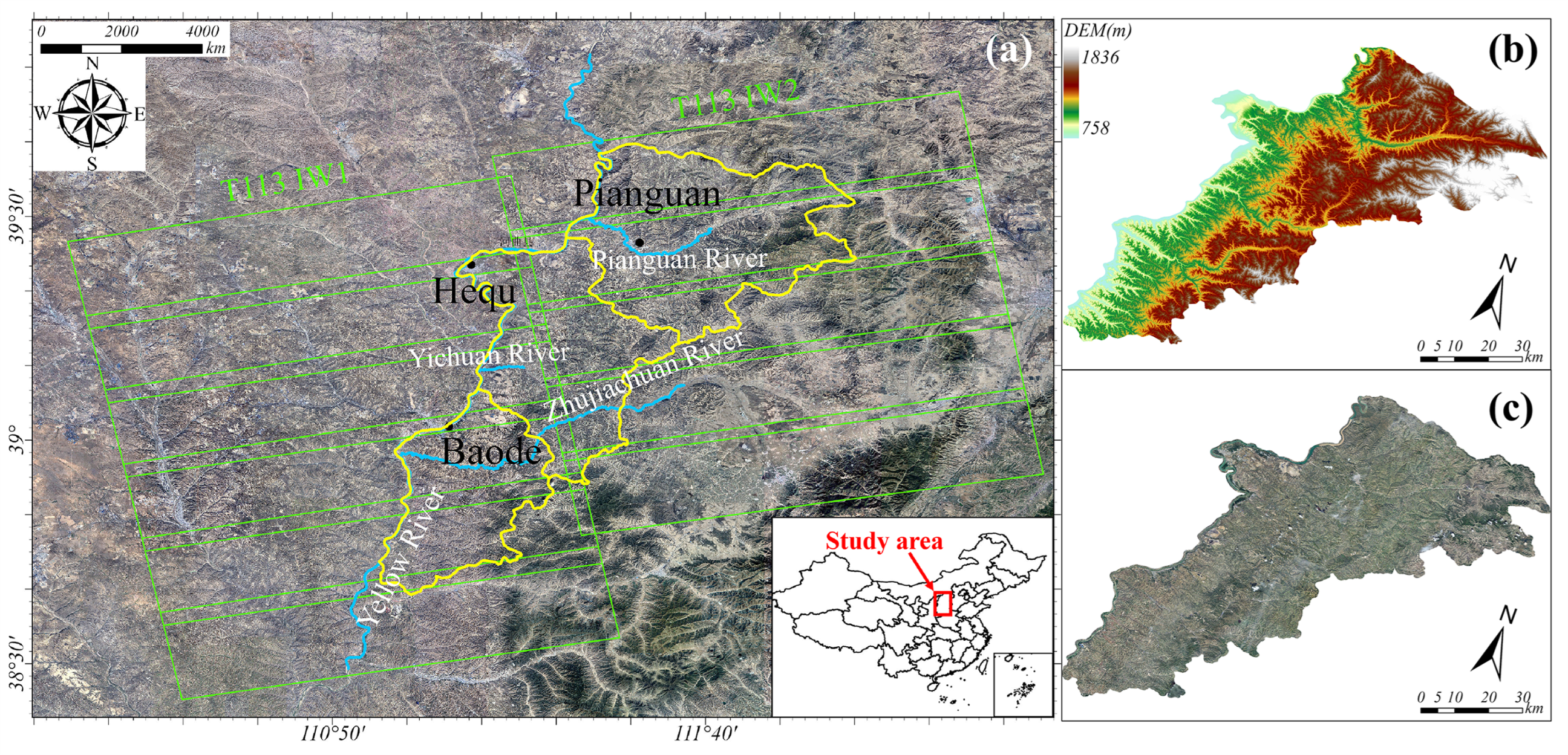
The Hequ–Baode–Pianguan (HBP) region is located within the boundaries of Xinzhou City in northwestern Shanxi Province, on the eastern bank of the Yellow River in the middle reaches of the Loess Plateau. It is a typical loess hilly and gully landform at the junction of the Shanxi, Shaanxi, and Inner Mongolia provinces [25]. The terrain of this region is higher in the east and lower in the west, with a large undulation. The average altitude is between 1000 and 1400 m. The climate type is a temperate continental monsoon climate, with an average annual temperature of about 3–9 °C. Precipitation is unevenly distributed in time and space, with an annual total of 350–470 mm, mainly concentrated in summer.

The HBP region is characterized by a thick loess layer over loose soil with poor resistance to erosion. The terrain is fragmented and crisscrossed with gullies. Geohazards occur frequently and are diverse in type, mainly including ground subsidence and landslides. The vegetation in this region is sparse, and the risk of desertification is prominent. It is prone to slope instability and soil erosion, with over 80% of the area affected. This region is a key area for ecological restoration in the Yellow River Basin [26]. At the same time, due to large-scale underground and open-pit mining of coal, bauxite, and other minerals (such as the Baode Coal Mine and the Hequ Iron Mine), abandoned mining areas in the region have been continuously expanding, leading to a series of ground subsidence and collapse events. The HBP region urgently needs to coordinate resource development and ecological restoration, and strengthen geohazard monitoring and comprehensive treatment to ensure the sustainable development of the regional economy and ecology. The study area is shown in Figure 1a.

2.2. Datasets

(1)

InSAR

For small study areas, downloading the full Sentinel-1 scene followed by preprocessing and cropping leads to unnecessary storage and computational costs. The Alaska Satellite Facility (ASF) platform enables burst-level downloading of Sentinel-1 data, significantly reducing storage usage and download time. Based on the study area, this study collected a total of 11 SAR data (bursts) from two Interferometric Wide swath (IW) modes of the Sentinel-1 satellite in the ascending orbit (T113) from October 2020 to June 2024. After conducting splicing, preprocessing, and cropping, a SAR image set covering the entire HBP area at 94 observation moments was obtained. The image information is shown in

Table 1. Information on the SAR images.

Sensor	Sentinel-1
Orbit number	T113
Acquisition time	202010-202406
Number of images (scenes)	94
IW	2
Burst	11

.

(2)

Optical remote sensing images

The remote sensing images used in this study are derived from the 0.5 m resolution optical image products of the SuperView-1 satellite series (Figure 1c). The dataset comprises 81 image scenes acquired in 2024, together with a true-color RGB product generated after color harmonization. Color, brightness, and contrast adjustments were applied to reduce tonal differences among the images. These data were used to identify PTOs and analyze PGH sites.

(3)

DEM

This study collected the SRTM global land DEM data covering the study area, processed by NASA and the National Geospatial-Intelligence Agency, with a spatial resolution of 30 m and an acquisition time of 2000, and used it as an external DEM to remove topographic effects from the InSAR phase. In addition, DEM data for the study area from the Japan Aerospace Exploration Agency’s ALOS satellite (Figure 1b) were obtained. The data, acquired from 2006 to 2011 at a spatial resolution of 12.5 m, were used to construct the geohazard terrain feature model.

(4)

Other data

(a)

Modified Normalized Difference Water Index (MNDWI)

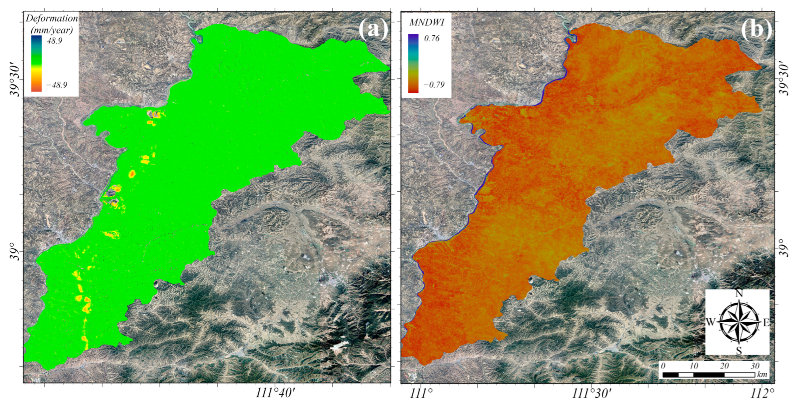
This study is based on the GEE platform and 20 m spatial-resolution Sentinel-2 multispectral data products from the European Space Agency. The average values of the green and short-wave infrared bands from May 2024 to November 2024 were extracted to calculate the MNDWI, which was used to filter out the active deformation areas (ADAs).

(b)

Vector data of road networks and mining areas

Road network and open-pit mine data were obtained from OpenStreetMap (OSM), a global volunteer-maintained geographic database. Vector data for roads, railways, and open-pit mines were downloaded from https://extract.bbbike.org using the research area selection and were used to establish the PTO database. In addition, vector data of mining subsidence areas surveyed in 2019 were collected and combined with open-pit mine data to analyze the spatial distribution of geological hazards.

3. Methodology

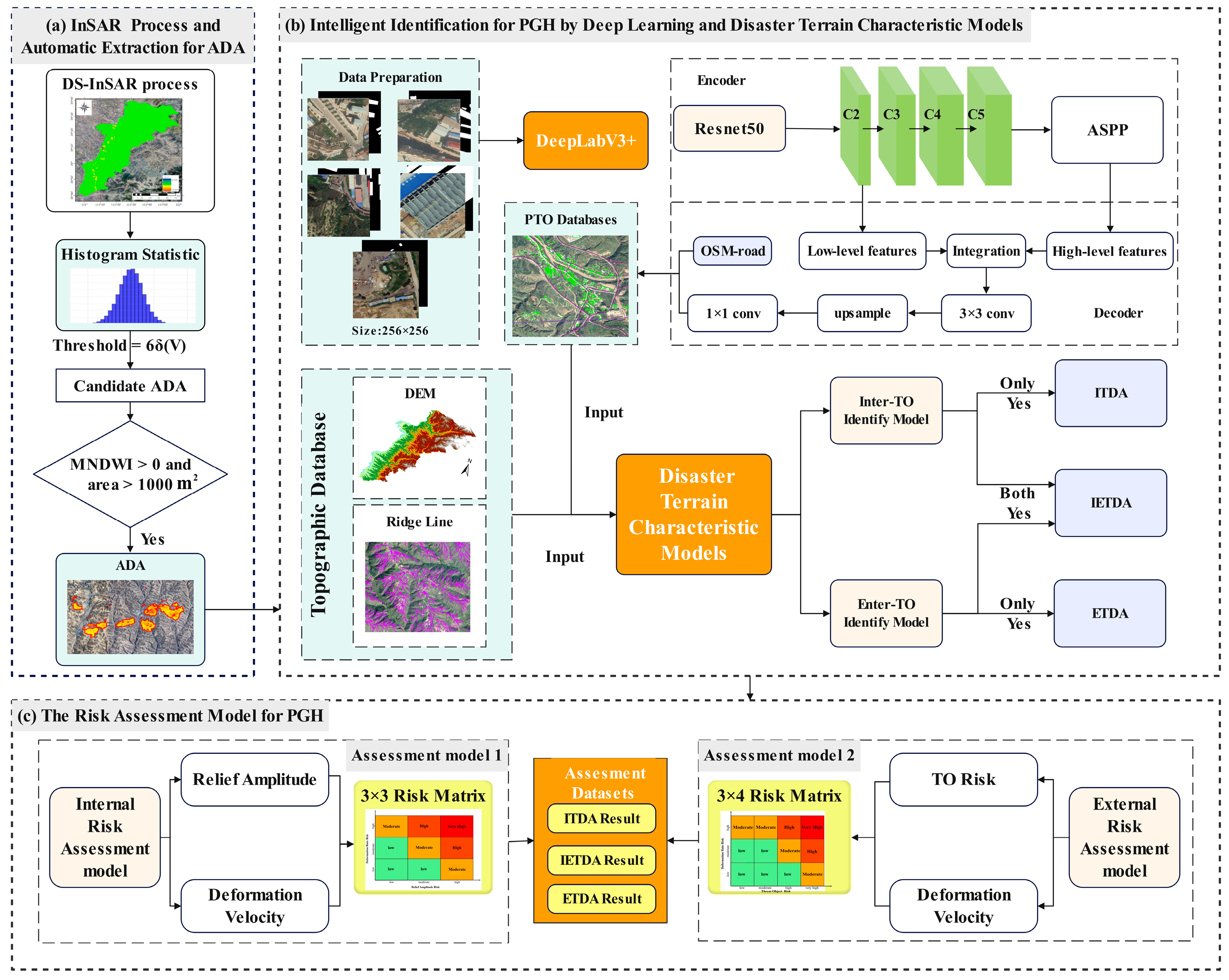
The main methods of this article include the following three sub-modules: (1) the method for wide-area monitoring and automatic extraction of ADAs based on InSAR; (2) automatic identification of PGHs combining TOs extracted using deep learning, multisource remote sensing data, and geohazard feature models; (3) risk assessment of PGHs. The method process is shown in Figure 2.

3.1. Wide-Area Deformation Monitoring and Automated Extraction of ADAs

3.1.1. Time-Series InSAR Deformation Monitoring

The Distributed Scatterer InSAR (DS-InSAR) integrates the point-target analysis concept of PS-InSAR with the small-baseline network of SBAS-InSAR, making it suitable for deformation monitoring in non-urban areas. Regression analysis is conducted on point targets to separate phase signals, including linear deformation, terrain residuals, atmospheric delays, and nonlinear deformation [27]. This approach overcomes the limitations of a single method regarding point-target density or spatial continuity, achieving better coverage of monitoring points and higher calculation accuracy.

The specific DS-InSAR process used in this paper is as follows. First, a temporal interferometric network is constructed from SAR image data. By setting the temporal and spatial baseline thresholds, we use all single-look complex SAR image sets to generate multi-temporal InSAR interferometric pairs. Subsequently, we select DS points based on the amplitude deviation index, time-series phase stability, and coherence. Then, phase filtering, terrain removal, and unwrapping are performed on all DS points [28,29]. In the interference processing stage, the time-series phases of the DS points are modeled using the Interferometric Point Target Analysis (IPTA) technique, and an observation equation incorporating deformation, terrain residual, and atmospheric delay terms is formulated. For high-coherence points, the interferometric phase of the pixel located at azimuth coordinate $x$ and range coordinate $r$ in the j-th interferogram, generated from a SAR image acquired at time $t_A$ and a master image acquired at time $t_B$$\left(t_A<t_B\right)$ can be written as:

$$\delta {\varphi }^j={\varphi }_B(x,r)-{\varphi }_A(x,r)\approx {\displaystyle \frac{4\pi }{\lambda }}\left[d\left(t_B,x,r\right)-d\left(t_A,x,r\right)\right]+\Delta {\varphi }_{topo}^j\left(x,r\right)+\Delta {\varphi }_{APS}^j\left(t_A,t_B,x,r\right)+\Delta {\varphi }_{noise}^j\left(x,r\right)$$

(1)

where $j\in \left(1,\dots ,M\right)$, and $\lambda$ is the radar signal central wavelength; $d\left(t_B,x,r\right)$ and $d\left(t_A,x,r\right)$ denote the cumulative line-of-sight (LOS) displacements at times $t_A$ and $t_B$, respectively, referenced to $d\left(t_0,x,r\right)=0$; $\Delta {\varphi }_{topo}^j\left(x,r\right)$ represents the residual topographic phase remaining in the differential interferogram [30], $\Delta {\varphi }_{APS}^j$ is the atmospheric phase screen contribution, and $\Delta {\varphi }_{noise}^j$ accounts for noise-related phase components. Subsequently, we used multiple linear regression to obtain the linear deformation, topographic residual, and residual phase. Then, by applying spatial and temporal-domain filtering methods, we separated the atmospheric delay phase from the nonlinear deformation phase. Finally, we combined the linear and nonlinear deformation components to obtain the final deformation.

3.1.2. Extraction of ADAs

Extracting ADAs from InSAR velocity requires first determining the accuracy or reliability of InSAR-derived deformation monitoring. We assume there is no deformation in the non-deforming area; that is, the deformation rate is 0. Then, the signal in the non-deforming area of the InSAR results is mainly due to observation error. The overall standard deviation of the deformation rate can be written as:

$$\delta \left(V\right)=\sqrt{{\displaystyle \frac{{\displaystyle \sum _{j=1}^N{\left[V\left(j\right)-\overline{V}\right]}^2}}{N-1}}}$$

(2)

where $\delta \left(V\right)$ is the standard deviation of the deformation rates of the N high-coherence points within the non-deformation area, with a total of N high-coherence points. $\overline{V}$ is the mean deformation rate within this area.

To enhance the reliability of the deformation monitoring results, we first select stable areas to calculate the mean deformation rate $\overline{V}$ by visual interpretation, as well as the standard deviation $\delta \left(V\right)$. The mean deformation rate $\overline{V}$ is used to estimate and correct the systematic offset of the LOS deformation-rate field, while the standard deviation $\delta \left(V\right)$ is used to determine the deformation-rate threshold for extracting ADAs. Subsequently, we set a threshold based on this standard deviation and the study area’s overall deformation characteristics to extract the vector range of the ADA domain initially. To reduce extraction errors due to noise, we use MNDWI [31] to screen the preliminary results. The calculation formula of MNDWI is as follows:

$$MNDWI={\displaystyle \frac{Green-SWIR}{Green+SWIR}}$$

(3)

where Green represents the green light band, and $SWIR$ is the short-wave infrared spectrum. Generally, areas with MNDWI values greater than 0 are considered water bodies [32]. Subsequently, we calculate the area of the ADAs and set a minimum area threshold of 1000 m². On this basis, we filter the initially extracted ADA vectors, retaining only areas with an average MNDWI of less than 0 and an area greater than 1000 m² as valid inputs for subsequent deformation classification and identification algorithms.

3.2. Automatic Identification of PGHs

3.2.1. Automatic Identification of PTOs Based on Deep Learning

The presence of TOs within or around an ADA is an important indicator for determining whether the ADA can be identified as a PGH. Accurate identification of all PTOs within the research area is a prerequisite. This study builds a DeepLabV3+ semantic segmentation model to extract PTOs from high-resolution optical remote sensing images [33]. The model follows an encoder–decoder architecture [34], with ResNet-50 serving as the encoder backbone for multi-level feature extraction. At the end of the encoder, an Atrous Spatial Pyramid Pooling (ASPP) module captures multi-scale contextual information in parallel using dilated convolutions with varying rates, complemented by global average pooling to derive image-level semantic features. The decoder fuses shallow detail features with the deep features output by ASPP, refines them with a 3 × 3 convolution, and then restores them to the original resolution via bilinear interpolation upsampling. Finally, a 1 × 1 convolution produces the segmentation result, enabling precise extraction of PTOs.

To address class imbalance in semantic segmentation, a composite loss function combining Dice loss and binary cross-entropy (BCE) loss was adopted. Dice loss optimizes segmentation boundaries by measuring the overlap between predicted and ground-truth masks, defined as:

$$L_{Dice}=1-{\displaystyle \frac{2{\displaystyle \sum _{i=1}^N{p}_i{g}_i+\in }}{{\displaystyle \sum _{i=1}^N{p}_i+{\displaystyle \sum _{i=1}^N{g}_i}+\in }}}$$

(4)

where $p_i$ is the predicted probability value, $g_i$ is the true label value, and $\in$ is a smoothing coefficient to prevent the denominator from being zero. Binary cross-entropy loss provides a pixel-wise classification error metric:

$$L_{BCE}=-{\displaystyle \frac{1}{N}}{\displaystyle \sum _{i=1}^N\left[g_i\log \left(p_i\right)+\left(1-g_i\right)\log \left(1-p_i\right)\right]}$$

(5)

The total loss function is a linear combination of the two terms defined above:

$$L_{total}=L_{Dice}+L_{BCE}$$

(6)

Subsequently, we create sample slices of the study area by manual visual interpretation and mark the corresponding binary masks through vectorization. The prepared image patches were divided into training and test sets using stratified sampling while maintaining geographic separation to reduce the influence of spatial autocorrelation.

We then evaluate the model using the following metrics: $Precision$, $Recall$, $F_1$, and $mIoU$. These metrics are calculated at the pixel level using macro averaging, in which the background and target classes are weighted equally. The corresponding equations are provided below.

$$Precision={\displaystyle \frac{1}{C}}{\displaystyle \sum _{i=1}^C\frac{T{P}_i}{T{P}_i+F{P}_i}}$$

(7)

$$Recall={\displaystyle \frac{1}{C}}{\displaystyle \sum _{i=1}^C\frac{T{P}_i}{T{P}_i+F{N}_i}}$$

(8)

$$F_1={\displaystyle \frac{1}{C}}{\displaystyle \sum _{i=1}^C\frac{2\times T{P}_{\mathrm{i}}}{2\times T{P}_i+F{P}_i+F{N}_i}}$$

(9)

$$mIoU={\displaystyle \frac{1}{C}}{\displaystyle {\displaystyle \sum _{i=1}^C}Io{U}_i}={\displaystyle \frac{1}{C}}{\displaystyle {\displaystyle \sum _{i=1}^C}\frac{T{P}_i}{T{P}_i+F{P}_i+F{N}_i}}$$

(10)

where $TP$, $FP$, and $FN$ respectively represent the quantities of true positives, false positives, and false negatives. $Io{U}_i$ is the intersection-over-union of the i-th category, and $C$ is the total number of categories (in this study, $C=2$). After training and evaluation, we apply the optimal model to the entire study area to generate a spatial distribution database of PTOs.

3.2.2. Extraction of Ridge Lines from High-Precision Digital Elevation Models

Ridge lines represent the connections between local elevation maxima on the terrain surface and reflect terrain undulation and drainage divides. They provide important information for geomorphic analysis, landslide morphology characterization, and PGH risk assessment. In PGH automatic identification, ridge lines are used to determine the terrain occlusion relationship between ADAs and PTOs. When ridge barriers exist, direct threats can be excluded even when the spatial distance is small. Therefore, accurate ridge line extraction is essential for improving the reliability of identification results.

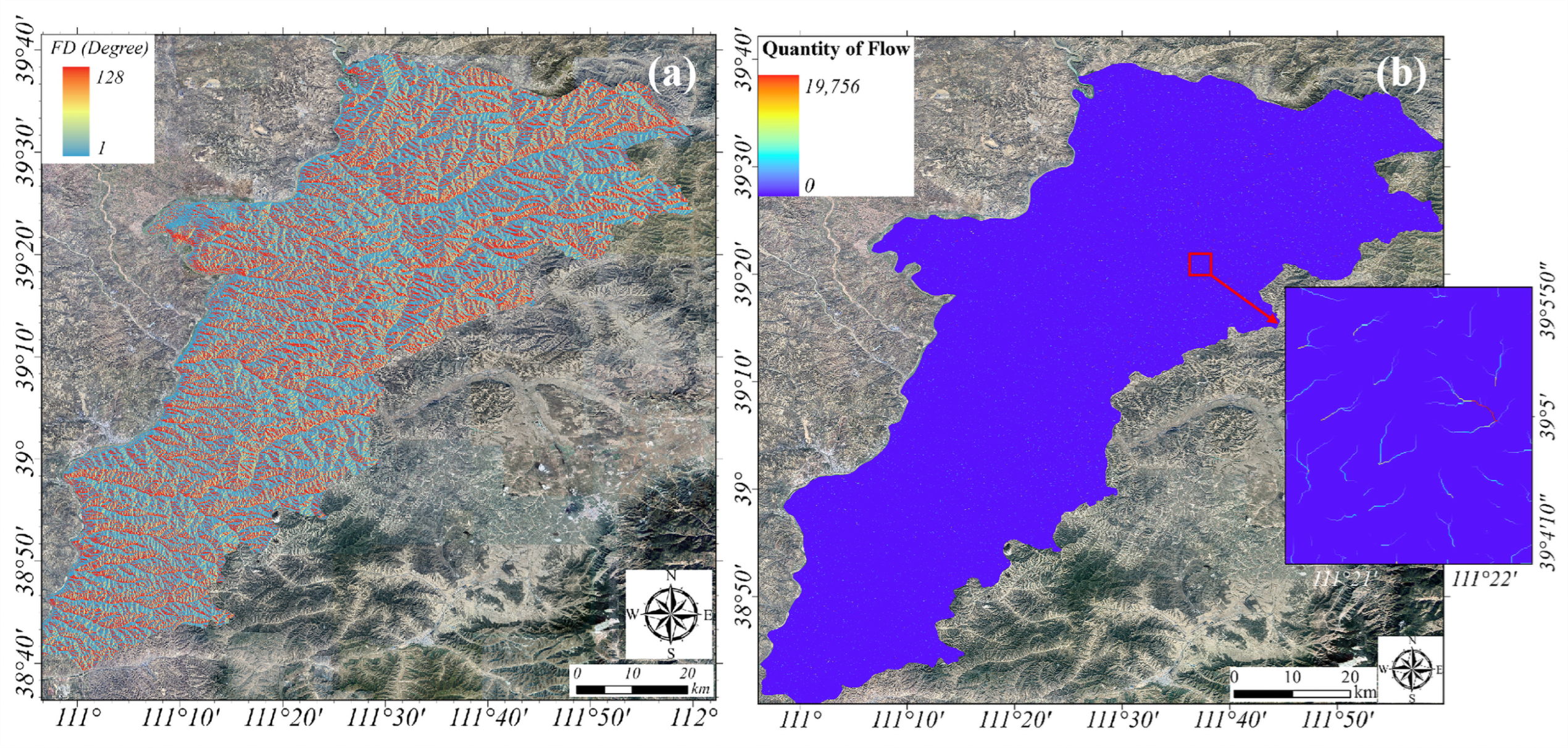
Based on topographic and hydrological analysis principles, ridge line extraction can be regarded as the reverse process of the catchment line. First, we invert the DEM to convert the ridges in the original terrain into low-lying areas. Then, based on the inverted DEM, we extract the ridge lines corresponding to the original flow direction (FD). The FD calculation uses the single-direction (D8) algorithm [35], taking a 3 × 3 window as the unit, and determines the FD of the central grid based on the maximum distance-weighted drop. Based on this, we calculate the upstream flow accumulation (FA) for each grid according to the laws of water flow. A larger FA indicates greater reverse confluence and a higher likelihood that the corresponding location represents a ridge line. Considering the terrain characteristics of the study area and the DEM resolution, this study adopts an adaptive flow threshold determination method based on statistical characteristics. First, we extract all valid flow pixel values greater than zero from the FA raster data and apply a logarithmic transformation to mitigate the skewness caused by high flow values. Then, we calculate the mode and standard deviation of the flow values after the logarithmic transformation using Equation (11).

$$T=\exp \left(mode+\eta \times \delta \left(FA\right)\right)-1$$

(11)

where $T$ is the ultimately determined FA threshold; $\delta \left(FA\right)$ is the standard deviation of the logarithmized FA; $\eta$ is the terrain condition coefficient. Adjusting this coefficient can adjust the formula’s adaptability to different terrain relief intensities. We extract pixel areas with FA exceeding the threshold as candidate ridge lines and then construct the ridge-line model of the study area by filtering and vector transformation.

3.2.3. Automatic Identification for PGHs

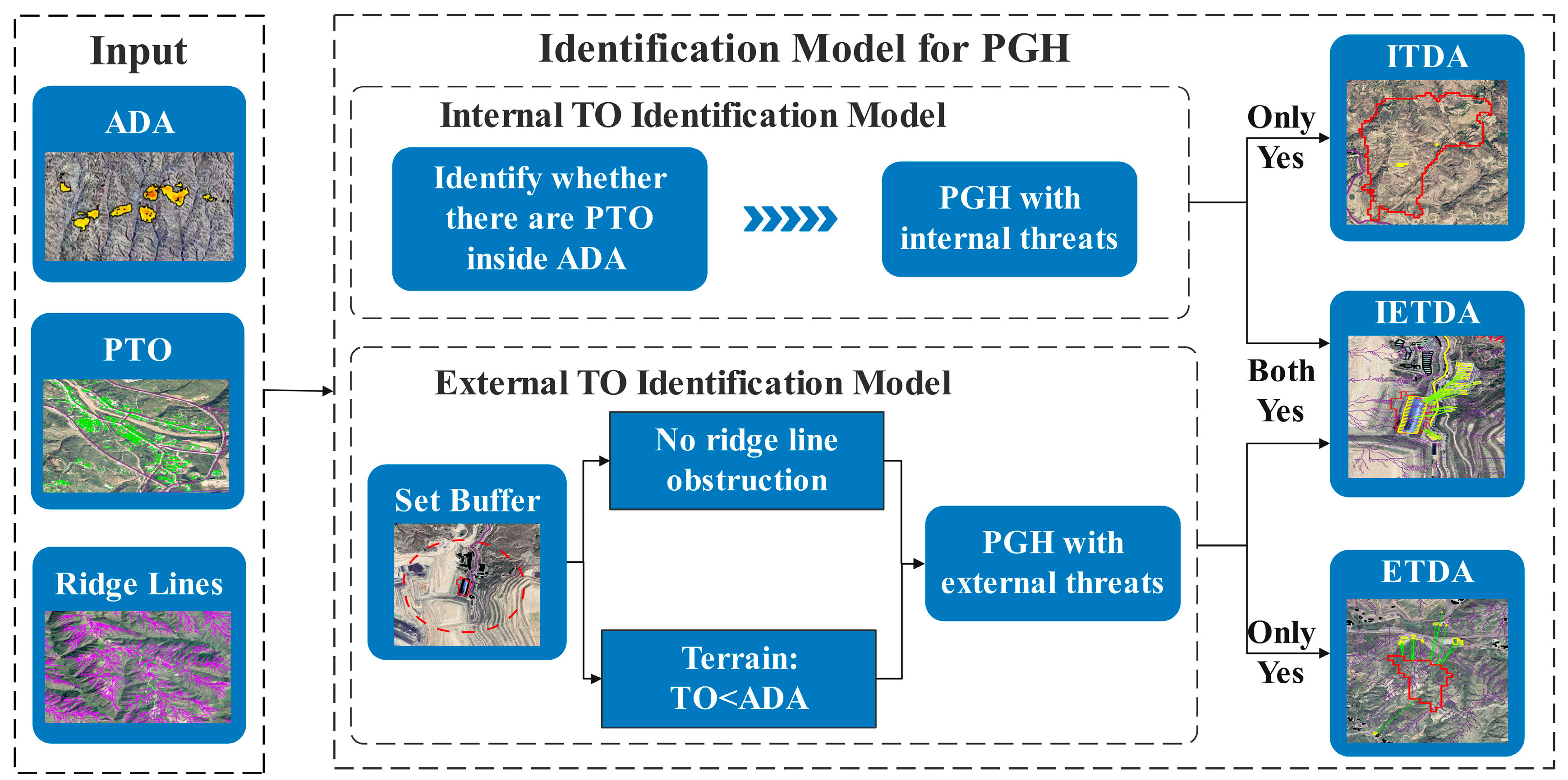
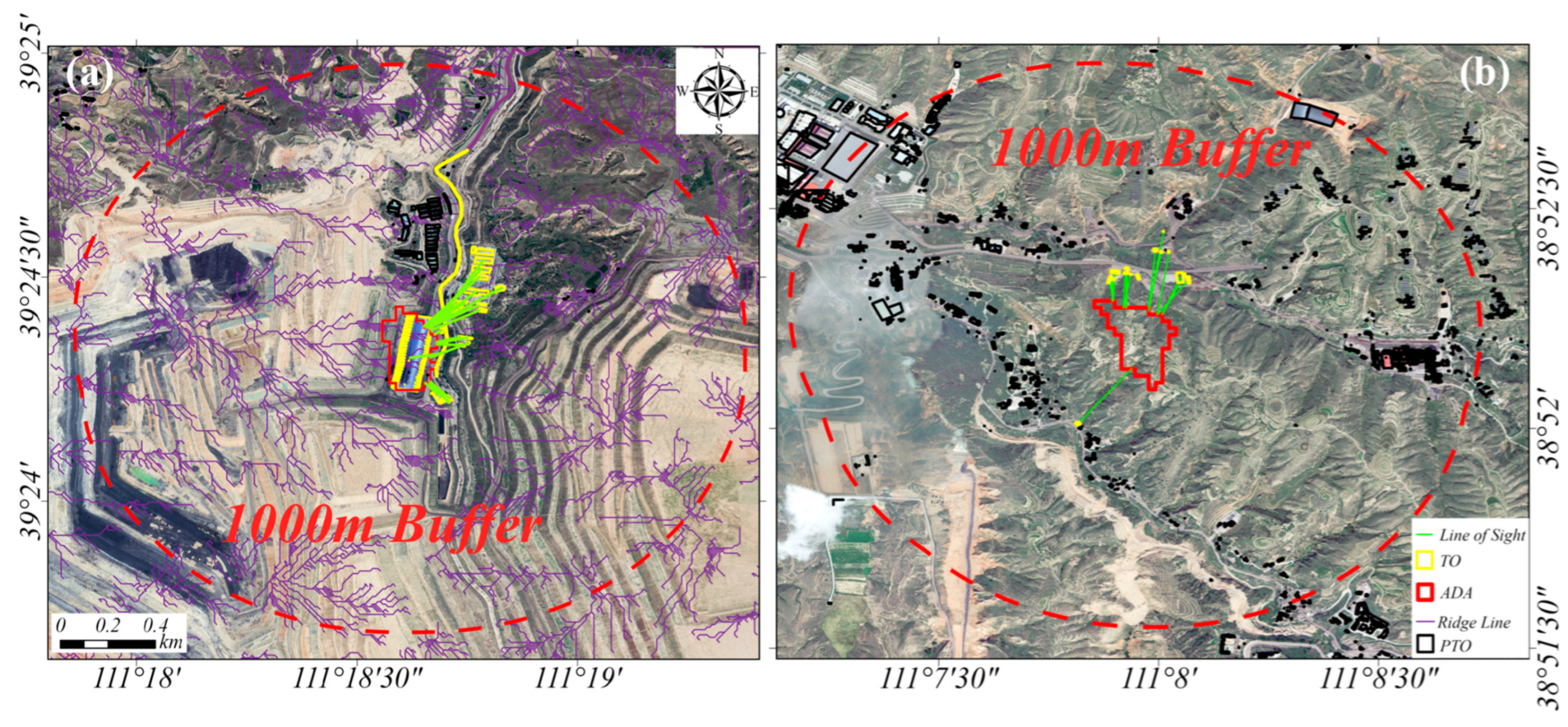
To automatically identify TOs both inside and outside ADAs, this study develops a PGH identification method that integrates deep learning results with a geohazard feature model (Figure 3). A PTO is identified as a threatened object (TO) when it is determined to be threatened by an ADA. We establish the internal TO identification model and the external TO identification model to concurrently identify whether an ADA has a TO and, based on this, determine whether they constitute PGH risks.

In the internal TO identification model, the ADA will be scanned. If we directly detect the PTOs identified by deep learning within the ADA, we will determine that the ADA is internally geohazard-causing. In the external TO identification model, we build the algorithm on the fundamental idea that there is terrain lower than the ADA within a certain range around the ADA, and no ridgeline blocks it. First, in accordance with the “Specification of risk assessment for geological hazard” (DZ/T 40112-2021) [36], we establish a buffer zone of 500 to 1000 m outside the ADA and retrieve the PTOs within it. For the PTOs within the buffer, the model will traverse them and conduct a more detailed assessment of whether they are under threat by further integrating the terrain line-of-sight occlusion relationship and relative elevation features. By extracting the ridge lines and conducting line-of-sight analysis, we determine whether any line-of-sight obstruction exists between the TO and the ADA. Meanwhile, we calculate the average elevation of the TO relative to the ADA based on the DEM. We determine that PTOs are threatened by the ADA only when they are not blocked by ridges in the line of sight and their average elevation is lower than that of the ADA. As long as the ADA identifies the TOs that meet the above requirements, it can be determined that the ADA is externally geohazard-causing.

An ADA containing at least one confirmed TO is identified as a PGH. Based on the spatial relationship between the TO and ADA, a PGH is further classified as an internal-threat deformation area (ITDA), an external-threat deformation area (ETDA), or an internal-external-threat deformation area (IETDA).

3.3. PGH Threat-Level Assessment and Prioritization

In this study, the risk assessment framework is oriented toward regional-scale geohazard screening and prioritization. It evaluates the relative threat level of potential geohazard candidates based on deformation characteristics, terrain conditions, and their spatial relationships with threatened objects.

3.3.1. Internal Risk Assessment Factor

For PGHs with internal TOs, this study conducts a risk assessment from two perspectives, i.e., relief amplitude in the spatial dimension and LOS deformation rate in the temporal dimension.

(1)

Relief amplitude factor

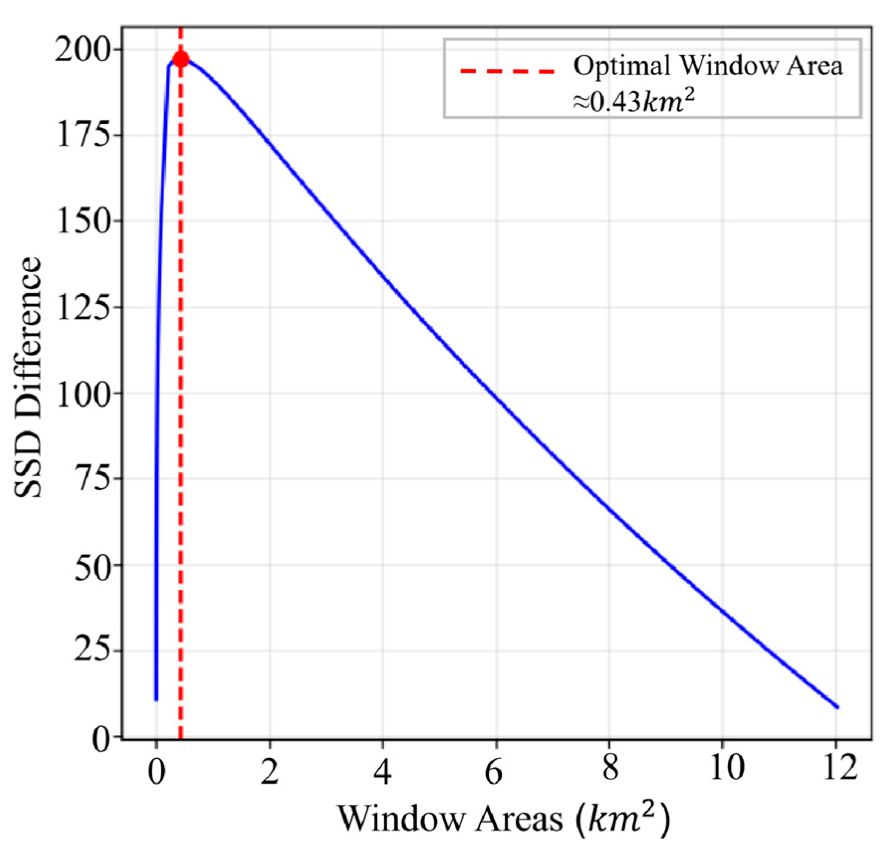
Relief amplitude (RA) refers to the elevation difference between the highest and lowest points within a specific area. This study uses the mean variation point method to determine the optimal statistical window area [37]. First, we determine the maximum window size and obtain the logarithmic sequence of the mean RA per unit area; then, we calculate the overall arithmetic mean and the sum of squared deviations using the least-squares method. Subsequently, we divide the data into two parts to calculate the mean and the sum of squared deviations (SSDs) for each group. Finally, the area corresponding to the maximum difference between the total sum of squared deviations and the group’s sum of squared deviations is taken as the optimal window area.

To reflect the positive correlation between RA and PGH risk, we set danger weights according to the landform types, so that higher relief corresponds to higher weights. According to the basic geomorphic classification principle of the first layer in China’s 1:1,000,000 Digital Geomorphological Classification Scheme, we divide the RA into four basic surface forms: plain (0–30 m), tableland (30–70 m), hilly land (70–200 m), and mountainous land (>200 m), which correspond to the weight values $P_j$ (j = 1,…, 4). Then, we traverse the extracted n ADAs and calculate the RA risk coefficient $X_i$ of the i-th ADA (where i = 1, 2, …, n).

$$X_i={\displaystyle \frac{{\displaystyle \sum _{j=1}^4\left(S_{ij}{P}_j\right)}}{S_i}}$$

(12)

Among them, $S_i$ is the area of the i-th ADA, $S_{ij}$ is the area of the j-th RA landform class within the i-th ADA, and $P_j$ is the corresponding weight. Based on the RA risk coefficient $X_i$, we use risk weights to divide it into different risk levels. The risk coefficient in the range of $\left[P_1,P_2\right]$ is defined as low risk, $\left[P_2,P_3\right]$ is moderate risk, and $\left[P_3,P_4\right]$ is high risk (

Table 2. Risk grade classification.

Type	RA Factor	Risk Grade	Deformation Rate Factor	Risk Grade
Internal Risk Factor Grade	$[{\mathrm{P}}_1,{\mathrm{P}}_2]$	Low risk	$V_{idex}<9\delta \left(V\right)$	Low risk
	$[{\mathrm{P}}_2,{\mathrm{P}}_3]$	Moderate risk	$9\delta \left(V\right)<V_{idex}<12\delta \left(V\right)$	Moderate risk
	$[{\mathrm{P}}_3,{\mathrm{P}}_4]$	High risk	$V_{idex}>12\delta \left(V\right)$	High risk
External Risk Factor Grade	$Y<{\mathsf{\epsilon }}_1$	Low risk	$\mid \overline{V}\mid <9\delta \left(V\right)$	Low risk
	${\mathsf{\epsilon }}_1<Y<{\mathsf{\epsilon }}_2$	Moderate risk	$9\delta \left(V\right)<\mid \overline{V}\mid <12\delta \left(V\right)$	Moderate risk
	${\mathsf{\epsilon }}_2<Y<{\mathsf{\epsilon }}_3$	High risk	$\mid \overline{V}\mid >12\delta \left(V\right)$	High risk
	Y $>{\mathsf{\epsilon }}_3$	Very high risk

).

(2)

Deformation rate factor

For the n ADAs, we successively extract the deformation-rate factors for each ADA. Then, for the k TOs within the i-th deformation, we construct a TO buffer for each. Finally, we calculate the average deformation rate within each buffer and select the buffer with the largest absolute value as the deformation rate evaluation index for this deformation. The equation for calculating the average deformation rate of the p-th TO buffer is:

$$V_p=\mathrm{mean}\left(V_{Buffer}\right)\left(p=1,2,\dots ,k\right)$$

(13)

where $V_p$ is the average value of the p-th TO deformation rate, and $V_{Buffer}$ is the deformation rate pixel value within the p-th TO buffer. Based on this, the deformation rate factor of the ADA i is defined as:

$$V_{idex}=\max \left(\left|V_1\right|,\left|V_2\right|,\cdots ,\left|V_k\right|\right)$$

(14)

Subsequently, based on the standard deviation δ(V) of the deformation rate obtained in Section 3.1, we set the risk level classification thresholds: $V_{idex}<9\delta \left(V\right)$ is low risk, $9\delta \left(V\right)<V_{idex}<12\delta \left(V\right)$ is medium risk, and $V_{idex}>12\delta \left(V\right)$ is high risk (Table 2). This is used to construct the grade gradient for the deformation-rate dimension in the internal risk assessment model.

3.3.2. External Risk Assessment Factor

For the ADA with TO on the outside, this study analyzes them from two perspectives: TOs in the spatial dimension and deformation rate in the temporal dimension.

(1)

TO factor

The distance from a PGH to a TO determines the attenuation of its kinetic energy, the complexity of its movement path, and the warning and response times. The height difference provides the potential energy of PGHs. We apply an external TO identification model to identify all the external TOs of the PGH. For the i-th PGH, we compute the distance and height difference between it and TOs and calculate the risk coefficient for the j-th TO of this ADA according to Equation (15).

$$Y_j={\displaystyle \frac{X}{D}}\times \Delta H\left(j=1,2,3\dots \right)$$

(15)

where $X$ is a distance adjustment parameter, empirically defined based on the PGH threat range in the study area to ensure an appropriate quantification range. The closer the distance and the greater the height difference, the higher the potential TO risk. Considering that an ADA may simultaneously have multiple external TOs, to conservatively assess the most unfavorable scenario, the TO risk coefficient Y for this ADA is defined as the maximum single-point risk coefficient by Equation (16).

$$Y=\max \left(Y_1,Y_2,\dots ,Y_j\right)$$

(16)

To clarify the risk gradient of the TO factor, we set three-level thresholds based on the statistical characteristics of the distance and height differences across all samples. During the propagation of geohazards, distance exerts greater influence than elevation differences. Therefore, we select the standard deviation of the distance and the gradient adjustment factor, and calculate the corresponding thresholds based on the sample mean distance and the mean elevation difference using Equations (17)–(19).

$${\epsilon }_1={\displaystyle \frac{X}{\overline{D}+{\delta }_{\mathit{distance}}}}\times \overline{\Delta H}$$

(17)

$${\epsilon }_2={\displaystyle \frac{X}{\overline{D}}}\times \overline{\Delta H}$$

(18)

$${\epsilon }_3={\displaystyle \frac{X}{\overline{D}-{\delta }_{\mathit{distance}}}}\times \overline{\Delta H}$$

(19)

Based on this, we divide the TO risk coefficient Y into four levels to serve as the TO risk-level classification index for the external risk assessment model. Among them, if it is less than ${\epsilon }_1$, it is classified as low risk; if it is between ${\epsilon }_1$ and ${\epsilon }_2$, it is classified as moderate risk; if it is between ${\epsilon }_2$ and ${\epsilon }_3$, it is classified as high risk; and if it is greater than ${\epsilon }_3$, it is classified as very high risk (Table 2).

(2)

Deformation rate factor

We calculated the average deformation rate $\left|\overline{V}\right|$ of each PGH with outside TOs to conduct the deformation rate dimension assessment. Subsequently, we classify $\left|\overline{V}\right|$ based on the deformation rate risk level index defined in Section 3.1. If $\left|\overline{V}\right|$ is less than $9\delta \left(V\right)$, it is classified as low risk; if it is between $9\delta \left(V\right)$ and $12\delta \left(V\right)$, it is classified as moderate risk; and if it is greater than $12\delta \left(V\right)$, it is classified as high risk (Table 2).

3.3.3. Integrated Threat-Level Assessment and Prioritization Model

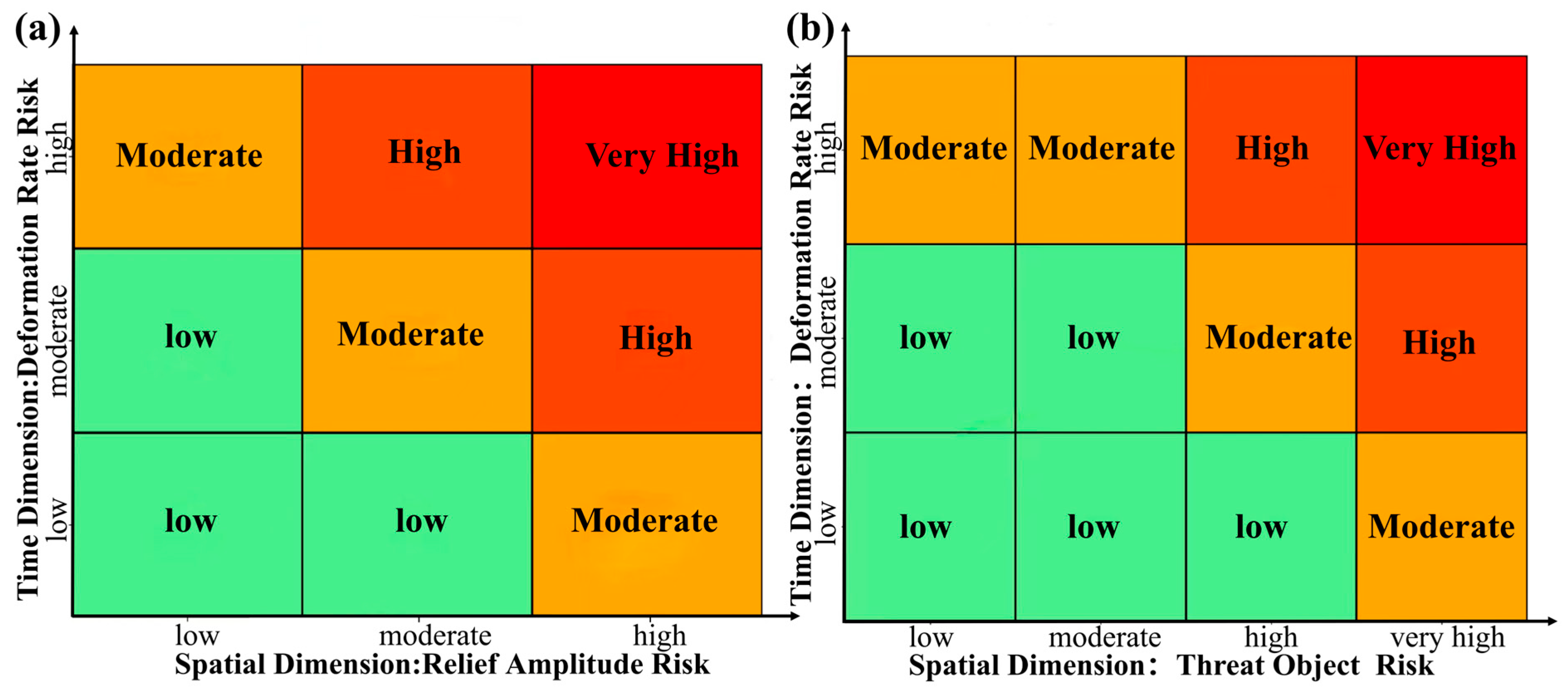
Based on the setting of risk assessment factors and risk gradients in Table 2, this study constructs a 3 × 3 risk matrix for the internal threat assessment model (Figure 4a) and a 3 × 4 risk matrix for the external threat assessment model (Figure 4b) to conduct a coupled analysis of risk characteristics in the time domain and the spatial domain, and it uses four risk levels to achieve an automated classification assessment of the PGH risks.

We use corresponding risk assessment models to determine the hazard level of different types of PGHs based on their threat characteristics. Among them, ITDAs use an internal risk assessment model, while ETDAs use an external one. For IETDAs, both models are used independently for assessment, and we take the higher risk level as their final risk level.

4. Data Processing and Results

4.1. Deformation Monitoring and Automated Extraction of ADAs

Firstly, we obtained the 11 burst data contained in T113 IW1 and IW2 covering the research area. After the format conversion, we performed preprocessing, such as registration and resampling, to ensure coordinate consistency. Based on the small-baseline strategy, the interferometric network was constructed by combining each acquisition with its three adjacent acquisitions to generate multi-temporal interferometric pairs [38]. We set the multi-look ratio in the range and azimuth directions to 4:1 for each interferogram pair to suppress noise. We used the external SRTM DEM to simulate the terrain phase signal and remove it from the interferometric phase [39]. Subsequently, we used DS-InSAR for time-series processing and extracted deformation results for the study area from 94 Sentinel-1 SAR images, as shown in Figure 5a.

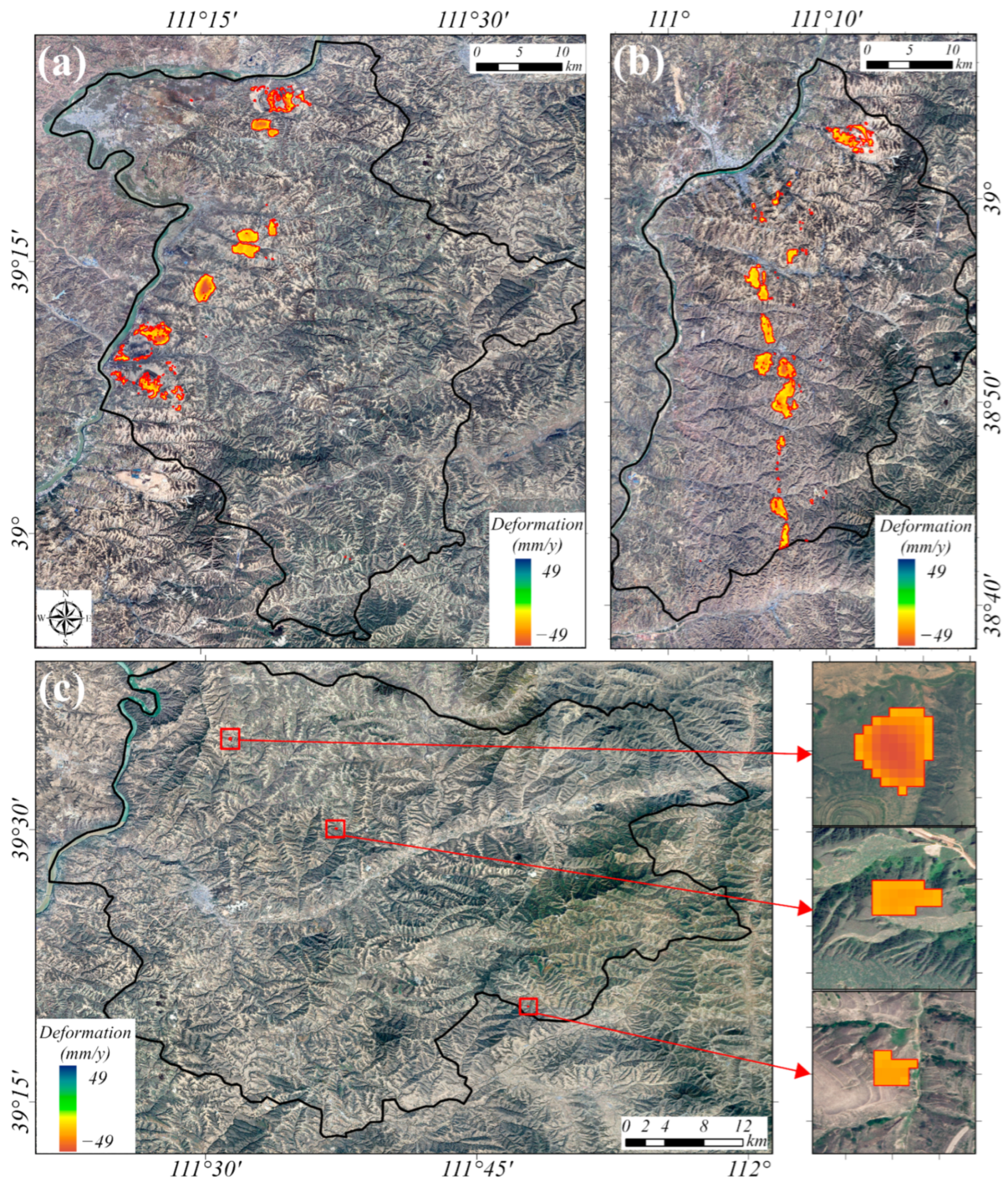
Based on the time-series deformation data of the study area, we initially extracted 224 candidate ADAs using a negative deformation-rate threshold of −6 $\delta \left(V\right)$, corresponding to −4.92 mm/year [40]. Then, we calculated the MNDWI in GEE (Figure 5b) and filtered the preliminary results using the preset ADA filtering conditions. Ultimately, 161 ADAs were determined (Figure 6).

4.2. Identification of PTOs Based on the DeepLabV3+ Model

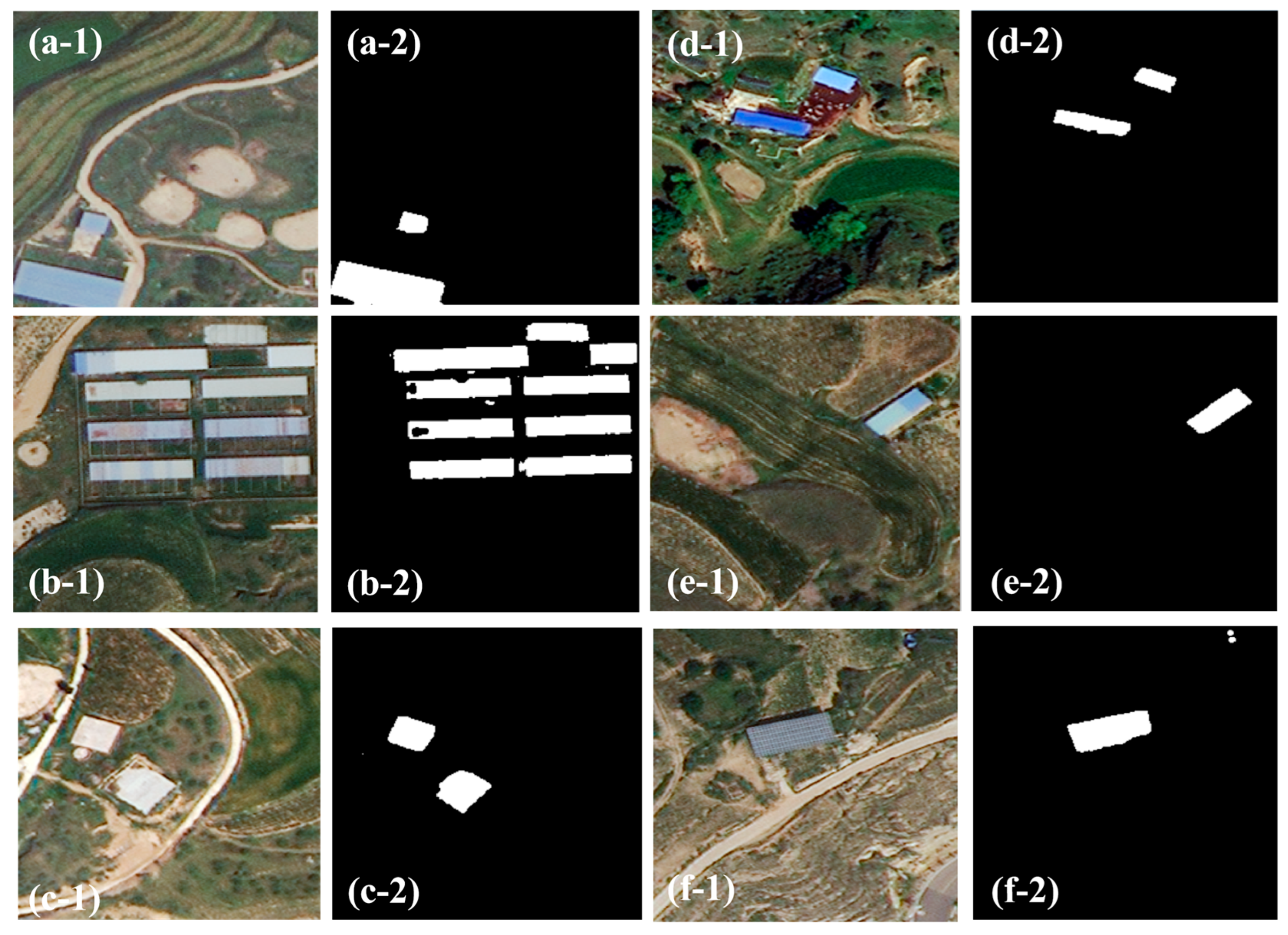
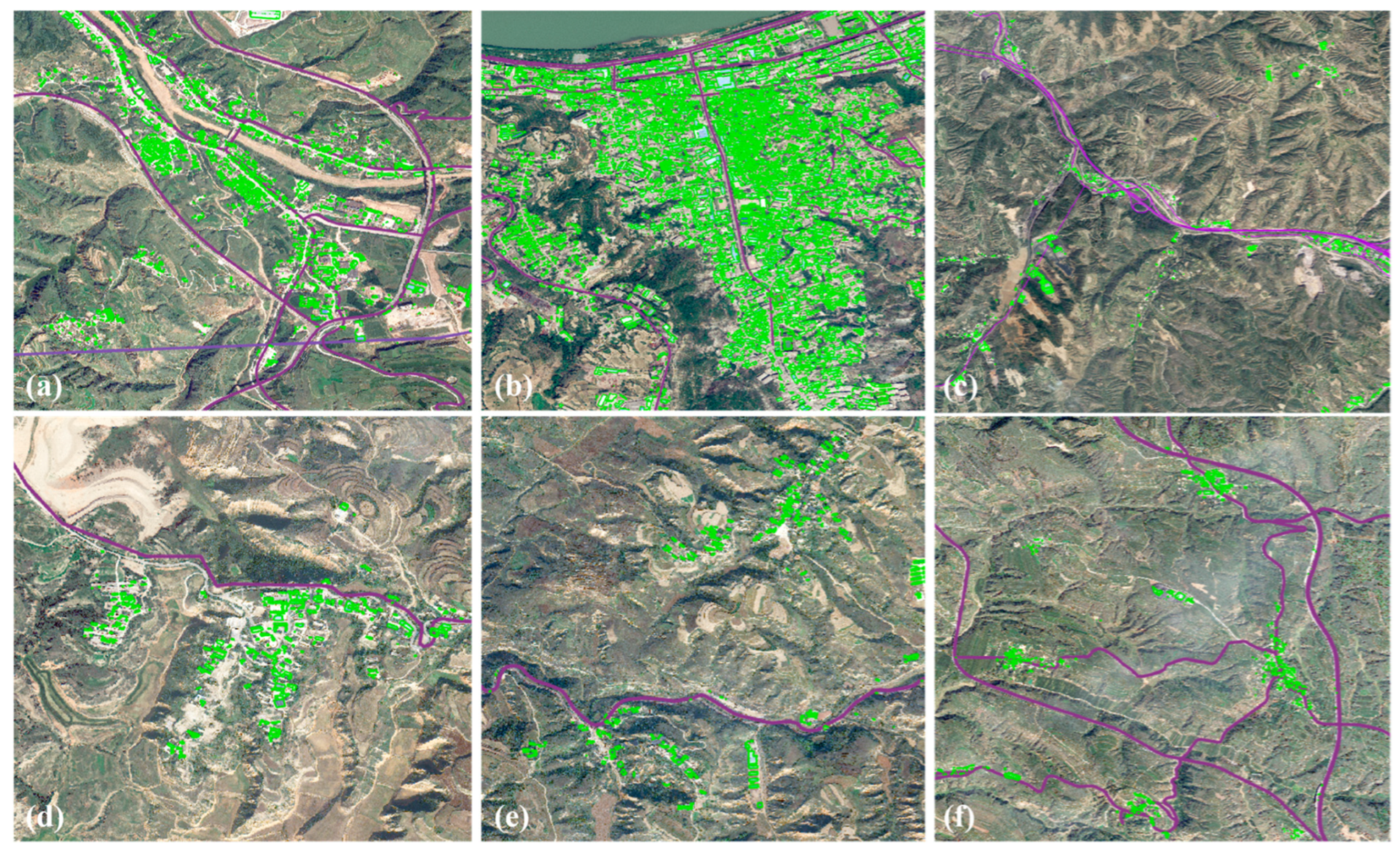
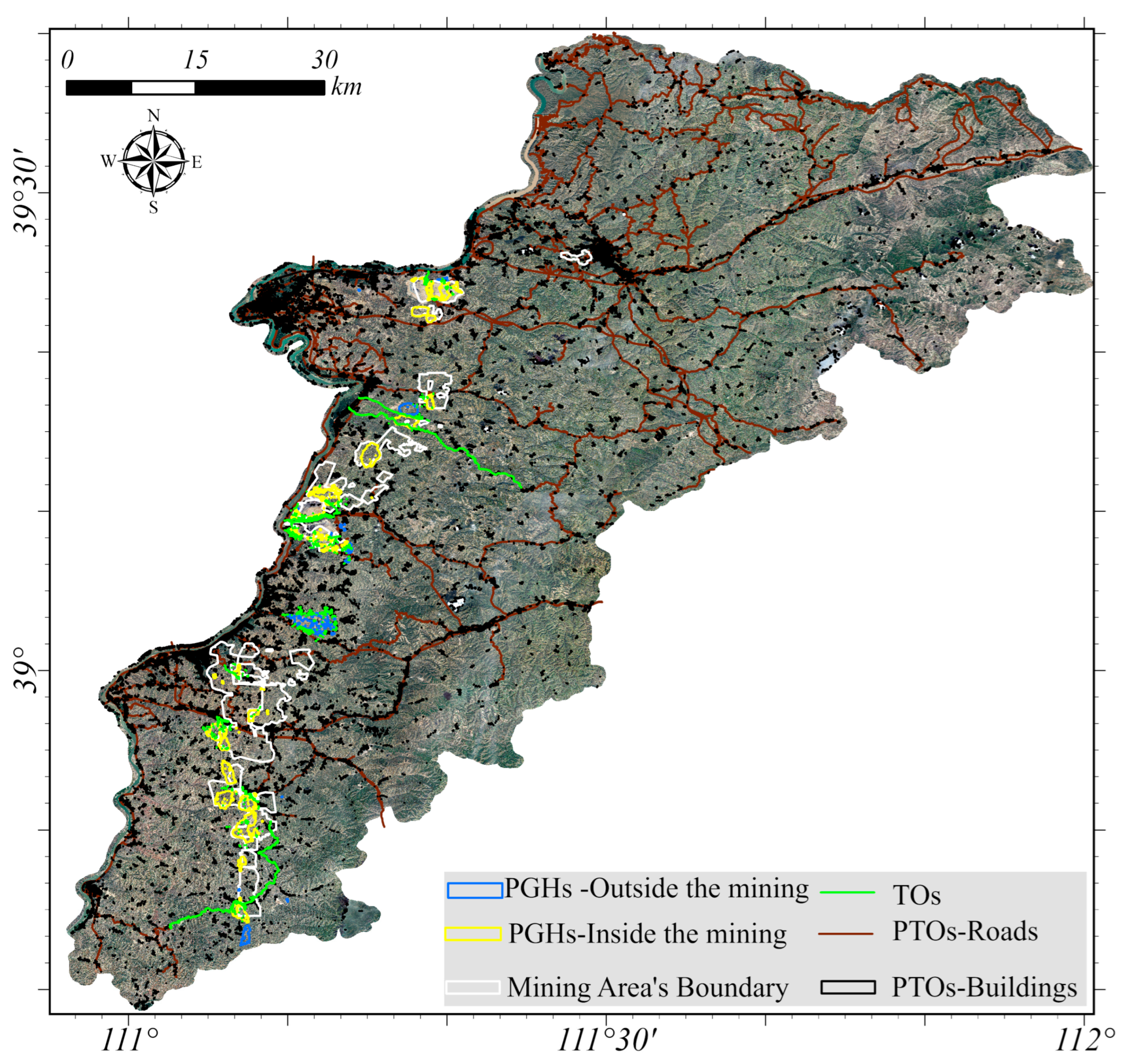
We conducted experiments by training a deep learning model on a device with an NVIDIA RTX 4090 GPU and 24 GB of RAM. We set the training process to 100 cycles and the batch size to 8. Then, we used 0.5 m resolution RGB optical remote sensing images covering the HBP area to create a sample library. We used manual visual interpretation to create samples, set target masks, and binarize the sample slices, with a target pixel value of 255 and a background pixel value of 0. Afterward, we cropped the sample area into 256 × 256-pixel slices, yielding 15,092 slices, including both positive and negative samples. Among them, there were 11,564 slices in the training set and 3528 slices in the test set. To evaluate the model, we used metrics such as $Precision$, $Recall$, $F_1$ and $mIoU$ (see

Table 3. Results of evaluation.

Metric	Value
$F_1$	0.907
$mIoU$	0.841
$Recall$	0.908
$Precision$	0.907

). This model achieved relatively high accuracy on the test set. Then, we made predictions after slicing all the images. Some of the prediction results are shown in Figure 7. Subsequently, we extracted and merged the target masks from the predicted binary images and cleaned the data for cloud clusters and noise points. Finally, we input the road network data and completed the construction of the PTO database for the study area, which included 142,619 buildings and 2138 road segments (Figure 8).

4.3. Identification for PGHs

(1)

Ridge line extraction

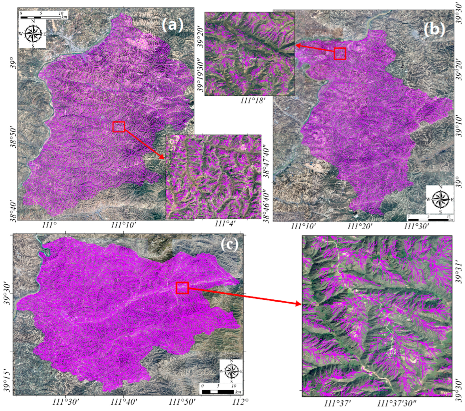
We extracted the ridgelines of the study area from the 12.5 m resolution ALOS DEM. We first preprocessed the DEM to ensure accurate and continuous extraction, including denoising and spatial correction. Subsequently, we inverted the DEM in ArcGIS Pro 3.1.6 and used the “Fill” tool to perform hydrological correction on the inverted DEM, eliminating false depressions and ensuring connectivity for the FD calculation. Based on the corrected inverted DEM, we used the D8 algorithm to calculate the FD (Figure 9a) and the FA (Figure 9b). We set the terrain adjustment coefficient to 1.5 and calculated the flow threshold T to be 22. Then, we binarized the flow data, extracted pixels exceeding the threshold as candidate ridge-line regions, and subsequently applied morphological filtering and connectivity analysis to smooth the linear shapes and vectorize them. Eventually, 943,090 ridge lines were extracted within the study area (Figure 10).

(2)

PGH identification results

We conducted a traversal analysis on the 161 ADAs extracted from the HBP area using the method described in Section 3.2 to identify PGHs and classify the threat types. Specifically, in the internal TO identification model based on spatial overlay analysis, we quickly determined the ITDA by intersecting the ADA and PTO surface elements. In the external TO identification model, we set a search radius of 1000 m and generated sampling points along the boundaries of ADAs and PTOs. Visibility is determined by whether the line connecting the two sampling points intersects the ridge-line vector. If all lines of sight are blocked, we determine that the PTO is shielded and not threatened by ADAs. If there are unobstructed lines of sight, we compare the PTO’s elevation to the ADA’s. If the PTO is a building, we directly calculate its average elevation for comparison; if the PTO is a road, we take the sampling point that passes the line-of-sight check as the center and extend a certain distance along the road on both sides to calculate the average elevation of the road’s local section. This study employed 5-pixel sizes, totaling 140 m. If both the line-of-sight detection and the terrain comparison meet the threat conditions, the model will identify the PTO as a TO. The algorithm traverses the PTO in increasing distance order. Once a TO that meets the conditions is identified, the search is terminated, and the ADA is determined to be an ETDA. Using this algorithm, we identified 90 PGHs in the HBP area, including 36 IETDAs (Figure 11a) and 54 ETDAs (Figure 11b).

4.4. Risk Assessment Results

When applying the internal risk assessment model, we used the mean variation point method to determine the optimal statistical window as 0.43 ${\mathrm{k}\mathrm{m}}^2$, as shown in Figure 12. Subsequently, we set the distribution interval weights of RA according to the landform types as $P_1=1$, $P_2=2$, $P_3=3$ and $P_4=4$ (

Table 4. Risk weighting for RA.

Geomorphic Type	RA (m)	${\mathit{P}}_{\mathit{j}}$
Plain	<30	$P_1$ = 1
Tableland	30 < RA < 70	$P_2$ = 2
Hilly land	70 < RA < 200	$P_3$ = 3
Mountain land	>200	$P_4$ = 4

), thereby reflecting the risk amplification effect in areas with high relief. Then, we calculated the RA risk coefficient by combining the proportion of each landform type in the ADA.

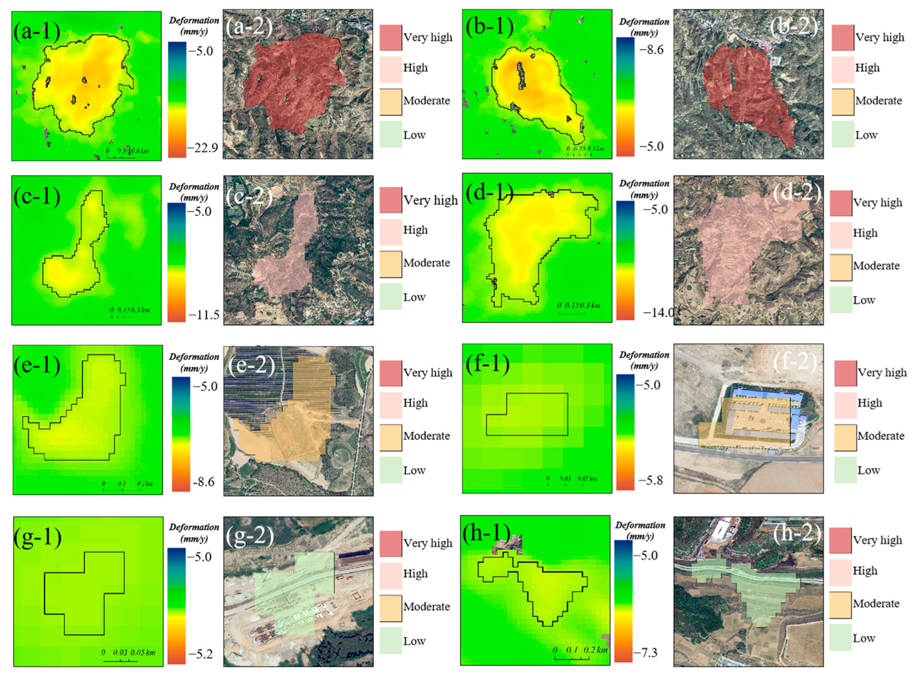
Within the PGH boundary, we set a 5-pixel buffer (140 m) for each TO to calculate the deformation rate factor. When applying the external risk assessment model, we used the external threat identification model to identify TOs, setting the search radius the same as in Section 4.3. Then, we set the distance adjustment parameter to 1000 and calculated the risk coefficient of the external TO factor. We assessed all PGHs for external threats and calculated the deformation rate at each PGH. Finally, based on the evaluation model in Section 3.3, we established a risk matrix to perform automated threat-level prioritization for PGH candidates. Based on the risk assessment, we classified 24 as low risk, 17 as moderate risk, 10 as high risk, and 3 as very high risk for ETDAs, as well as 1 as low risk, 6 as moderate risk, 11 as high risk, and 18 as very high risk for IETDAs (

Table 5. Risk assessment results for PGHs.

PGH Types	Low-Risk	Moderate-Risk	High-Risk	Very High-Risk
ETDA	24	17	10	3
IETDA	1	6	11	18

). Partial risk assessment results are shown in Figure 13.

5. Discussion

5.1. Surface Deformation in Coal Mining Areas and Its Response to PGH Risks

Shanxi Province has significant coal reserves, and multiple coal mining areas are located within the HBP region (Figure 14). Mining subsidence is one of the main factors causing surface instability in the HBP area. Studying the distributional characteristics of surface deformation and associated PGH risks in mining areas will contribute to safe production and ecological health in mines. Mining subsidence typically follows distinct spatial development patterns [41] and significantly impacts the surface within a certain range around the mining area [42]. Therefore, this section focuses on the internal area of the HBP mining district as the key research object and discusses the identification of PGH risks associated with mining subsidence, along with their characteristics.

We conducted a spatial topological analysis on the vector boundaries of the mining area, ADAs, PTOs, etc. Surface deformation is highly concentrated in certain areas of the mining area. We extracted a total of 99 ADAs within the mining area, accounting for 61.5% of the total unstable areas in the study area. Among them, 58 were in coal-mining subsidence areas and 41 in open-pit mining areas. Applying the method in 3.2 to identify these ADAs, we found that 59 ADAs were PGHs, accounting for 59.6% of the ADAs in the mining area, slightly higher than the proportion of ADAs converted into PGHs in the entire area (55.9%). There are 26 IETDAs, of which 92.3% are high-risk areas, and 33 ETDAs, of which 33.3% are high-risk areas (

Table 6. Statistics of PGHs.

Category		PGHs in Open-Pit Mining	PGHs in Coal Mining Subsidence
PGH areas	Very high-risk ETDA	0	3
	High-risk ETDA	3	5
	Moderate-risk ETDA	5	5
	Low-risk ETDA	2	10
	Very high-risk IETDA	8	9
	High-risk IETDA	3	4
	Moderate-risk IETDA	2	0
	Low-risk IETDA	0	0
	In total	23	36
Non-PGH areas		18	22

).

It can be seen that PGH risk levels in the mining area are generally high, and special attention should be paid to the PGH risks posed by overlying buildings and structures during production and operation. In addition to the PTO analysis, we identified 5114 PTOs within the HBP mining area boundary. Among them, there were 181 internal TOs (accounting for 3.5%) and 392 external TOs (accounting for 7.7%) in the HBP region. In addition, 97 buildings and one road are located both inside and outside multiple PGHs, thus subject to compound threats. This indicates that the engineering facilities in the mining area and its surroundings have been subjected to the cumulative effects of multiple surface deformations for a long time. In contrast, the proportions of TOs within and outside the geohazard-stricken areas in PTOs across the entire region were 0.39% and 1.54%, respectively, both lower than those in mining areas. In conclusion, the surface instability areas within the mining area are more prone to developing PGHs, with significant potential to cause geohazards. High-risk and very-high-risk IETDAs should therefore be prioritized in subsequent management and risk control for mining areas. The number of ADAs, the proportion of IETDAs, and the density of internal TOs within the mining area boundaries are all higher than those in non-mining areas, indicating that coal mining activities are closely associated with the spatial distribution of PGHs.

Although the management of PGH risks in mining areas is not the traditional focus of PGH prevention and control, the above results have direct guiding significance for safe production in mining areas and the management of the geological environment. Based on the precise identification of ADAs and high-risk hidden dangers within the mining area, quantitative evidence can be provided to support the regulation of mining intensity, the optimization of the mining area layout, and post-mining zonal restoration. This helps shift from “post-event governance” to “risk pre-control”, demonstrating the method’s potential for application in the comprehensive management of the geological environment in mining areas.

5.2. The Application Prospects of PGH Intelligent Mapping Using Multisource Remote Sensing

This study develops an automated algorithm for PGH identification and risk assessment by integrating multisource remote sensing data and deep learning. This method integrates time-series InSAR wide-area deformation monitoring, high-resolution optical remote sensing intelligent interpretation, and the establishment of geohazard feature models, achieving full-process automation from the automatic delineation of unstable surface areas and the automatic identification of PTOs to hazard and risk screening and assessment. Compared with traditional approaches that rely on manual interpretation and field surveys, the proposed method significantly reduces time and economic costs during the early investigation stage. In practical applications, only regional multisource remote sensing monitoring data and necessary thresholds need to be input into the model, and it can automatically output the PGHs to focus on and their risk-level assessment results. This shifts limited resources from large-scale screening to targeted verification, thereby supporting efficient, risk-driven field investigation and mitigation. The proposed framework provides strong technical support for improving the efficiency of wide-area PGH early identification and risk management.

This study combines high-resolution optical imagery with topographic data to conduct expert visual interpretation, providing additional evidence for evaluating the reliability of the identified potential geohazard candidates. Considering the regional-scale application of this framework, further validation using multisource independent datasets, such as field surveys, UAV observations, or existing geological hazard inventories, would be valuable to further assess its robustness and transferability. Therefore, the results presented in this study are primarily intended as a regional-scale screening and prioritization product, providing a basis for identifying key areas and supporting subsequent detailed investigations. In addition, the current assessment framework mainly focuses on the relative threat level from the perspective of deformation characteristics, terrain conditions, and spatial relationships with threatened objects. Factors related to vulnerability, socioeconomic exposure, and potential losses are not explicitly incorporated, which could be further considered in future studies to extend the framework toward more comprehensive quantitative risk assessment.

6. Conclusions

This study proposes a method for automatic identification and risk assessment of PGHs using multisource remote sensing data and deep learning algorithms. This method has been applied and evaluated in HBP. By processing 94 Sentinel-1 SAR scenes covering the HBP area using DS-InSAR and automatic deformation extraction, we obtained surface deformation for the area from 2020 to 2024 and extracted 161 ADAs. The DeepLabV3+ model was used to perform semantic segmentation on 0.5 m resolution optical images, thereby constructing a PTO database covering the study area. By integrating terrain, ridge lines, and spatial topological relationships, we established an internal and external TO identification model, achieving automatic screening and classification of PGHs. Based on the constructed model and ADA identification results, we have identified 90 PGH candidates in the HBP region, including 36 IETDAs and 54 ETDAs. By establishing internal and external threat prioritization models and introducing a risk matrix, we classified the relative threat levels of PGH candidates in the HBP region as 25 low risk, 23 moderate risk, 21 high risk, and 21 very high risk. Ultimately, this study systematically analyzed the surface deformation in the coal mining area and the transformation of PGHs. By comparing relevant indicators of PGHs within and outside the mining area, it was found that mining activities are closely associated with the spatial distribution of PGHs, providing a scientific basis for environmental restoration and safe production management in the mining area. Note that, as a methodological study, this work primarily emphasizes the development and operational implementation of the integrated algorithmic workflow. At the same time, the accuracy of its outputs is expected to improve correspondingly with higher-quality input data. If future experimental platforms become more advanced, we will further validate the method’s accuracy. The method proposed in this study can provide technical support for the census, identification, and risk assessment of PGHs in the Loess Plateau and similar PGH-prone areas, and support regional geohazard screening, investigation planning, and intelligent supervision.

References

1. Xu, Q.; Zhao, B.; Dai, K.; Dong, X.; Li, W.; Zhu, X.; Yang, Y.; Xiao, X.; Wang, X.; Huang, J.; et al. Remote sensing for landslide investigations: A progress report from China. Eng. Geol. 2023, 321, 107156–107182. [Google Scholar] [CrossRef] [Scilit]
2. Raspini, F.; Caleca, F.; Del Soldato, M.; Festa, D.; Confuorto, P.; Bianchini, S. Review of satellite radar interferometry for subsidence analysis. Earth-Sci. Rev. 2022, 235, 104239–104278. [Google Scholar] [CrossRef] [Scilit]
3. Ma, P.; Lin, H.; Wang, W.; Yu, H.; Chen, F.; Jiang, L.; Zhou, L.; Zhang, Z.; Shi, G.; Wang, J. Toward Fine Surveillance: A review of multitemporal interferometric synthetic aperture radar for infrastructure health monitoring. IEEE Geosci. Remote Sens. Mag. 2020, 10, 207–230. [Google Scholar] [CrossRef] [Scilit]
4. Yang, Z.; Li, Z.; Zhu, J.; Wang, Y.; Wu, L. Use of SAR/InSAR in Mining Deformation Monitoring, Parameter Inversion, and Forward Predictions: A Review. IEEE Geosci. Remote. Sens. Mag. 2020, 8, 71–90. [Google Scholar] [CrossRef] [Scilit]
5. Dai, K.; Li, Z.; Xu, Q.; Burgmann, R.; Milledge, D.G.; Tomas, R.; Fan, X.; Zhao, C.; Liu, X.; Peng, J.; et al. Entering the Era of Earth Observation-Based Landslide Warning Systems: A Novel and Exciting Framework. IEEE Geosci. Remote Sens. Mag. 2024, 8, 136–153. [Google Scholar] [CrossRef] [Scilit]
6. Qu, F.; Zhang, Q.; Lu, Z.; Zhao, C.; Yang, C.; Zhang, J. Land subsidence and ground fissures in Xi’an, China 2005–2012 revealed by multi-band InSAR time-series analysis. Remote Sens. Environ. 2014, 155, 366–376. [Google Scholar] [CrossRef] [Scilit]
7. Dong, J.; Zhang, L.; Li, M.; Yu, Y.; Liao, M.; Gong, J.; Luo, H. Measuring precursory movements of the recent Xinmo landslide in Mao County, China with Sentinel-1 and ALOS-2 PALSAR-2 datasets. Landslides 2017, 15, 135–144. [Google Scholar] [CrossRef] [Scilit]
8. Dong, J.; Niu, R.; Li, B.; Xu, H.; Wang, S. Potential landslides identification based on temporal and spatial filtering of SBAS-InSAR results. Geomat. Nat. Hazards Risk 2022, 14, 52–75. [Google Scholar] [CrossRef] [Scilit]
9. Liu, Y.; Yao, X.; Gu, Z.; Li, R.; Zhou, Z.; Liu, X.; Jiang, S.; Yao, C.; Wei, S. Research on automatic recognition of active landslides using InSAR deformation under digital morphology: A case study of the Baihetan reservoir, China. Remote Sens. Environ. 2024, 304, 114029. [Google Scholar] [CrossRef] [Scilit]
10. Yao, J.; Wang, T.; Yao, X. Spatial-temporal evolution of landslides spanning the impoundment of Baihetan mega hydropower project revealed by satellite radar interferometry. Remote Sens. Environ. 2025, 321, 114668. [Google Scholar] [CrossRef] [Scilit]
11. Dai, C.; Zhang, S.; Zhong, L.; Xue, D.; Fang, Z.; Zhou, Y.; Li, W. A slow-moving landslide risk assessment procedure using thematic maps and InSAR data: A case study. Georisk Assess. Manag. Risk Eng. Syst. Geohazards 2025, 19, 730–750. [Google Scholar] [CrossRef] [Scilit]
12. Tian, F.; Zhang, W.; Zhu, H.-H.; Wang, C.; Chang, F.-N.; Li, H.-Z.; Tan, D.-Y. Multi-temporal InSAR-based landslide dynamic susceptibility mapping of Fengjie County, Three Gorges Reservoir Area, China. J. Rock Mech. Geotech. Eng. 2025, 17, 7653–7664. [Google Scholar] [CrossRef] [Scilit]
13. Zhu, Y.; Chen, H.; Sun, D.; Zhu, X.; Ji, Q.; Wen, H.; Zhang, Q.; Wu, R. A heterogeneous ensemble landslide susceptibility assessment method based on InSAR and geographic similarity extended landslide inventory. Gondwana Res. 2025, 144, 181–196. [Google Scholar] [CrossRef] [Scilit]
14. Liu, Z.; Qiu, H.; Yang, S.; Zhou, C.; Zhang, L.; Zhou, C.; Zhu, Y.; Ma, S. Two-decadal evolution of irreversible surface deformation in a coal mining area revealed by improved InSAR observations. Catena 2025, 254, 108996. [Google Scholar] [CrossRef] [Scilit]
15. Yi, Z.; Liu, M.; Liu, X.; Wang, Y.; Wu, L.; Wang, Z.; Zhu, L. Long-term Landsat monitoring of mining subsidence based on spatiotemporal variations in soil moisture: A case study of Shanxi Province, China. Int. J. Appl. Earth Obs. Geoinf. 2021, 102, 102447. [Google Scholar] [CrossRef] [Scilit]
16. Ouyang, C.; An, H.; Zhou, S.; Wang, Z.; Su, P.; Wang, D.; Cheng, D.; She, J. Insights from the failure and dynamic characteristics of two sequential landslides at Baige village along the Jinsha River, China. Landslides 2019, 16, 1397–1414. [Google Scholar] [CrossRef] [Scilit]
17. Liu, X.; Zhao, C.; Zhang, Q.; Lu, Z.; Li, Z.; Yang, C.; Zhu, W.; Liu-Zeng, J.; Chen, L.; Liu, C. Integration of Sentinel-1 and ALOS/PALSAR-2 SAR datasets for mapping active landslides along the Jinsha River corridor, China. Eng. Geol. 2021, 284, 106033. [Google Scholar] [CrossRef] [Scilit]
18. Zhao, C.; Chen, L.; Yin, Y.; Liu, X.; Li, B.; Ren, C.; Liu, D. Failure process and three-dimensional motions of mining-induced Jianshanying landslide in China observed by optical, LiDAR and SAR datasets. GISci. Remote Sens. 2023, 60, 2268367. [Google Scholar] [CrossRef] [Scilit]
19. Su, X.; Zhang, Y.; Meng, X.; Rehman, M.U.; Yue, D.; Zhao, Y.; Zhou, Z.; Guo, F.; Zhou, Q.; Niu, B. An integrated landslide susceptibility assessment in the Karakoram Mountains based on SBAS-InSAR and machine learning: A case study of the Hunza Valley. Bull. Eng. Geol. Environ. 2025, 84, 280. [Google Scholar] [CrossRef] [Scilit]
20. Han, W.; Zhang, X.; Wang, Y.; Wang, L.; Huang, X.; Li, J.; Wang, S.; Chen, W.; Li, X.; Feng, R.; et al. A survey of machine learning and deep learning in remote sensing of geological environment: Challenges, advances, and opportunities. ISPRS J. Photogramm. Remote Sens. 2023, 202, 87–113. [Google Scholar] [CrossRef] [Scilit]
21. Ji, S.; Yu, D.; Shen, C.; Li, W.; Xu, Q. Landslide detection from an open satellite imagery and digital elevation model dataset using attention boosted convolutional neural networks. Landslides 2020, 17, 1337–1352. [Google Scholar] [CrossRef] [Scilit]
22. Anantrasirichai, N.; Biggs, J.; Kelevitz, K.; Sadeghi, Z.; Wright, T.; Thompson, J.; Achim, A.M.; Bull, D. Detecting Ground Deformation in the Built Environment Using Sparse Satellite InSAR Data with a Convolutional Neural Network. IEEE Trans. Geosci. Remote Sens. 2021, 59, 2940–2950. [Google Scholar] [CrossRef] [Scilit]
23. Ju, Y.; Xu, Q.; Jin, S.; Li, W.; Su, Y.; Dong, X.; Guo, Q. Loess Landslide Detection Using Object Detection Algorithms in Northwest China. Remote Sens. 2022, 14, 1182. [Google Scholar] [CrossRef] [Scilit]
24. Cai, J.; Ming, D.; Liu, F.; Ling, X.; Liu, N.; Zhang, L.; Xu, L.; Li, Y.; Zhu, M. Change detection of slow-moving landslide with multi-source SBAS-InSAR and Light-U2Net. Int. J. Appl. Earth Obs. Geoinf. 2025, 136, 104387. [Google Scholar] [CrossRef] [Scilit]
25. Hao, C. Research on Land Use in Pianguan County from the Perspective of County Development. Master’s Thesis, Shanxi Agricultural University, Jinzhong, China, 2019. [Google Scholar]
26. Zhang, K. Spatio-Temporal Variation Characteristics and Influencing Factors of Ecosystem Services in Xinzhou. Master’s Thesis, Shanxi University, Taiyuan, China, 2023. [Google Scholar]
27. Wang, Y.; Feng, G.; Li, Z.; Yang, Z.; Wang, B.; Wang, Y.; Du, Y.; Wang, Y.; He, L.; Zhu, J. A multi-frame deformation velocity splicing method for wide-area InSAR measurement based on uncontrolled block adjustment: A case study of long-term deformation monitoring in Guangdong, China. Remote Sens. Environ. 2024, 301, 113929. [Google Scholar] [CrossRef] [Scilit]
28. Li, Z.-W.; Ding, X.-L.; Zheng, D.-W.; Huang, C. Least Squares-Based Filter for Remote SensingImage Noise Reduction. IEEE Trans. Geosci. Remote Sens. 2008, 46, 2044–2049. [Google Scholar] [CrossRef]
29. Goldstein, R.M.; Werner, C.L. Radar interferogram filtering for geophysical applications. Geophys. Res. Lett. 1998, 25, 4035–4038. [Google Scholar] [CrossRef] [Scilit]
30. Lanari, R.; Mora, O.; Manunta, M.; Mallorqui, J.J.; Berardino, P.; Sansosti, E. A small-baseline approach for investigating deformations on full-resolution differential SAR interferograms. IEEE Trans. Geosci. Remote Sens. 2004, 42, 1377–1386. [Google Scholar] [CrossRef] [Scilit]
31. Xu, H. Modification of normalised difference water index (NDWI) to enhance open water features in remotely sensed imagery. Int. J. Remote Sens. 2007, 27, 3025–3033. [Google Scholar] [CrossRef] [Scilit]
32. Vijay, A.; Varija, K. Spatio-temporal classification of land use and land cover and its changes in Kerala using remote sensing and machine learning approach. Environ. Monit. Assess. 2024, 196, 459. [Google Scholar] [CrossRef] [Scilit]
33. Xu, B.; Cai, D.; Shi, J.; Sui, K.; Tang, W.; Liu, C. SAG-DeepLabV3+: An Enhanced Deep Learning Model forHigh-Precision Detection of Mining-Induced Ground Fissuresfrom UAV Imagery. Remote Sens. 2026, 18, 2388. [Google Scholar] [CrossRef] [Scilit]
34. Abbas, S.; Almadhor, A.; Sampedro, G.A.; Alsubai, S.; Al Hejaili, A.; Strážovská, Ľ.; Zaidi, M.M. Efficient geospatial mapping of buildings, woodlands, water and roads from aerial imagery using deep learning. PeerJ Comput. Sci. 2024, 10, e2039. [Google Scholar] [CrossRef] [Scilit]
35. Fairfield, J.; Leymarie, P. Drainage networks from grid digital elevation models. Water Resour. Res. 1991, 27, 709–717. [Google Scholar] [CrossRef] [Scilit]
36. GB/T 40112-2021; Specifications for Risk Assessment of Geological Hazard. State Administration for Market Regulation, China National Standardization Administration: Beijing, China, 2021.
37. Deng, J.; Cheng, W.; Liu, Q.; Jiao, Y.; Liu, J. Morphological differentiation characteristics and classification criteria of lunar surface relief amplitude. J. Geogr. Sci. 2022, 32, 2365–2378. [Google Scholar] [CrossRef] [Scilit]
38. Paolo, B.; Gianfranco, F.; Riccardo, L.; Eugenio, S. A New Algorithm for Surface Deformation Monitoring Based on Small Baseline Differential SAR Interferograms. IEEE Trans. Geosci. REMOTE Sens. 2003, 40, 2375–2383. [Google Scholar] [CrossRef] [Scilit]
39. Wang, Y.; Feng, G.; Li, Z.; Xu, W.; Wang, H.; Hu, J.; Liu, S.; He, L. Estimating the long-term deformation and permanent loss of aquifer in the southern Junggar Basin, China, using InSAR. J. Hydrol. 2022, 614, 128604. [Google Scholar] [CrossRef] [Scilit]
40. Luo, S.; Feng, G.; Xiong, Z.; Wang, H.; Zhao, Y.; Li, K.; Deng, K.; Wang, Y. An Improved Method for Automatic Identification and Assessment of Potential Geohazards Based on MT-InSAR Measurements. Remote Sens. 2021, 13, 3490. [Google Scholar] [CrossRef] [Scilit]
41. Li, Z.W.; Yang, Z.F.; Zhu, J.J.; Hu, J.; Wang, Y.J.; Li, P.X.; Chen, G.L. Retrieving three-dimensional displacement fields of mining areas from a single InSAR pair. J. Geod. 2014, 89, 17–32. [Google Scholar] [CrossRef] [Scilit]
42. Wang, Y.; Yang, Z.; Li, Z.; Zhu, J.; Wu, L. Fusing adjacent-track InSAR datasets to densify the temporal resolution of time-series 3-D displacement estimation over mining areas with a prior deformation model and a generalized weighting least-squares method. J. Geod. 2020, 94, 47. [Google Scholar] [CrossRef] [Scilit]
Figure 1. (a) Overview of the study area (the yellow line marking the boundary of the study area and the green line indicating the coverage of Sentinel-1 satellite images). (b) ALOS Satellite DEM Product. (c) Remote sensing image of SuperView-1 with 0.5 m resolution.
Remotesensing 18 02890 g001
Figure 2. Flowchart of the research methodology.
Remotesensing 18 02890 g002
Figure 3. Flowchart of PGH identification.
Remotesensing 18 02890 g003
Figure 4. (a) Risk matrix of the internal threat assessment model. (b) Risk matrix of the external threat assessment model.
Remotesensing 18 02890 g004
Figure 5. (a) The LOS deformation rate results in the HBP region from 2020 to 2024. (b) Average MNDWI results.
Remotesensing 18 02890 g005
Figure 6. (a) Extraction results for ADAs in Hequ, (b) Baode, and (c) Pianguan.
Remotesensing 18 02890 g006
Figure 7. Prediction of buildings in the research area. (a-1f-2) Representative samples of building extraction results; (1) high-resolution optical remote sensing images; (2) corresponding building prediction masks generated by the DeepLabV3+ model.
Remotesensing 18 02890 g007
Figure 8. Database of PTOs in the study area (the green borders represent the identified building vectors, and the purple lines represent the road network).
Remotesensing 18 02890 g008
Figure 9. (a) Flow direction; (b) flow accumulation.
Remotesensing 18 02890 g009
Figure 10. (a) Extracted results of the ridge lines in Baode, (b) Hequ, and (c) Pianguan.
Remotesensing 18 02890 g010
Figure 11. (a) IETDA; (b) ETDA.
Remotesensing 18 02890 g011
Figure 12. Mean variation point analysis.
Remotesensing 18 02890 g012
Figure 13. Representative threat-level assessment results of potential geohazard candidates. (a-1h-2) Representative cases: (1) deformation-rate maps; (2) corresponding high-resolution optical remote sensing images.
Remotesensing 18 02890 g013
Figure 14. Topological relationship between mining subsidence areas and PGHs in the HBP region.
Remotesensing 18 02890 g014