Radargrammetric 3D Positioning of Pseudo Corner-Reflector Scatterers in KOMPSAT-5 Stacks with Per-Target Conditioning Diagnostics

Highlights

What are the main findings?

• An integrated pseudo-CR pipeline (CFAR ranked by local contrast, multi-scale templates, and multi-look range-Doppler triangulation with per-target conditioning diagnostics) reaches 0.7–2.9 m 3D accuracy on nine KOMPSAT-5 Mongolia corner reflectors.
• At a corner-reflector-absent suburban site, 16 surveyed distribution poles that formed stable multi-scene responses are positioned to a mean horizontal difference of 3.19 m from the surveyed pole base; on that response-enriched set, ranking candidates by local contrast retains more of those responses than ranking by absolute power at equal candidate budgets.

What are the implications?

• Natural pole-like scatterers that form stable multi-scene responses and can be associated with a specific structure are candidate reference features where no dedicated CRs exist.
• Per-target conditioning diagnostics, adapted from stereo-SAR practice to mid-resolution KOMPSAT-5 stacks, describe how well the observing geometry determines each solution and flag weak conditioning where no ground control is available.

Abstract

Spaceborne synthetic aperture radar (SAR) needs point-like reference targets for co-registration, calibration, and absolute geolocation, but real corner reflectors (CRs) exist only at a few dedicated sites. We present a detection and three-dimensional (3D) positioning pipeline for naturally occurring corner-reflector-like (pseudo-CR) scatterers in KOMPSAT-5 stacks, combining constant false alarm rate (CFAR) detection ranked by local contrast rather than absolute power, a multi-scale template bank, multi-look range-Doppler bundle triangulation, and a per-target conditioning diagnostic vector. At the nine-CR Mongolia calibration field, all nine are recovered, with a mean horizontal error of 1.37 m and a mean 3D error of 2.01 m. At a CR-absent suburban site in Suncheon, Republic of Korea, 18 scenes yield 39,822 clusters, 26,659 of which pass the conditioning gate. Over 16 response-enriched poles retained by author adjudication, the difference to the nearest conditioning-filtered cluster averages 3.19 m horizontally and 1.45 m vertically relative to the surveyed pole base. Because part of that set was selected after inspecting preliminary responses, these are conditional nearest-cluster agreements, not verified target accuracies, and no detection probability is claimed. In an exploratory comparison on the same set, contrast ranking retains more evaluation targets than power ranking at equal budgets, 16 against 9 of 16. Removing robust weighting and pruning degrades the mean Mongolia 3D error to 7.39 m; the DEM prior is non-critical, whereas the clustering radius is consequential in the dense pole field, with the count within 20 m falling from 16 to 9 as the radius grows from 15 m to 30 m. In a leave-scene-out check, 85.8% of 254 evaluable clusters persist in a scene excluded from their solutions, against 35.2% of 270 evaluable random positions: a complete-case enrichment of 78%, or 53–82% under cross-arm worst-case imputation of the unevaluable targets; neither estimate measures catalogue precision. Limited KOMPSAT-5 stacks can therefore yield few-metre nearest-cluster agreement at selected pole locations where stable multi-scene responses form.

1. Introduction

Synthetic aperture radar (SAR) provides all-weather imaging for registration, change analysis and geolocation. Deployed corner reflectors (CRs) provide strong reference targets for absolute SAR calibration and positioning [1], while feature-based registration methods such as SAR-SIFT, OS-SIFT and radiation-invariant transforms address image-to-image alignment without deployed targets [2,3,4]. This study instead seeks stable natural scatterers that can be positioned in three dimensions from a limited set of KOMPSAT-5 scenes.

Real CRs are deployed at only a few calibration sites, so they cannot provide dense reference coverage for routine registration or geolocation. Naturally occurring stable, point-like scatterers are a practical alternative, but they must be detected in clutter and observed from sufficiently diverse geometries. This study therefore combines local-contrast candidate detection with multi-scene range-Doppler (RD) triangulation to position such pseudo-CR scatterers without using ground control in the solution.

Recovering 3D coordinates requires more than locating a bright pixel in one image. Each observation supplies range and zero-Doppler constraints; their intersection is sensitive to look-angle diversity, residual delay and the location of the physical scattering centre. The pipeline therefore attaches per-target geometric and residual diagnostics to each bundle solution and evaluates them against surveyed targets where available.

Spatial resolution also limits the observable target structure and the attainable geolocation accuracy. Spotlight and sliding-spotlight SAR can reach approximately metre-scale resolution [5,6,7], whereas the standard KOMPSAT-5 scenes used here are mostly 2.5–3 m. The present work therefore addresses the mid-resolution regime rather than claiming the centimetre-level performance demonstrated with very-high-resolution TerraSAR-X data [8].

This work contributes to the limited-stack, mid-resolution branch of the problem with KOMPSAT-5 (K5) imagery [9]. The objective is twofold: (a) extract pseudo-CR-like point scatterers from a small number of K5 standard-mode Single-Look Complex (SLC) scenes covering an arbitrary area, including suburban regions without CRs; (b) compute 3D coordinates for those scatterers, validate them against external ground control where available, and attach intrinsic per-target conditioning diagnostics that require no ground control. The specific contributions of this paper are:

Here, a limited stack means a tasking-driven, geometrically heterogeneous set rather than a co-registered single-geometry PSI time series; the Suncheon and Mongolia stacks contain 18 and 39 scenes, respectively.

• An integrated pseudo-CR extraction pipeline combining CFAR detection ranked by local contrast ratio rather than by absolute power, a multi-scale point/plus/cross template bank with optional bright-pixel size and area gates, sub-pixel peak refinement, and rigorous range-Doppler geocoding. Window and template sizes may be given in pixels or in metres and are converted per scene from the H5 spacings, so that a single processing chain handles the mixed ground sampling distance (1.0–3.0 m) of the stacks used here. Section 4.4.1 shows that the ranking criterion, rather than the choice of CFAR variant, is what makes weak pole responses survive to the triangulation stage.
• A multi-look RD bundle triangulation framework that converts clusters of co-located detections across scenes into single 3D points. The implementation supports robust weighting and residual-based outlier pruning against a median-scaled residual threshold, while permissive runs can keep two-observation clusters to evaluate weak pseudo-CR candidates.
• A per-target conditioning diagnostic vector combining observation count, RD residual RMS, height conditioning, look-angle spread and the normal-matrix condition number. Such descriptors are established in stereo-SAR practice [8,10]; the contribution here is their evaluation in the mid-resolution KOMPSAT-5 regime.
• Two-site validation: nine surveyed Mongolia CRs provide absolute truth, while 16 response-enriched Suncheon poles provide conditional nearest-cluster agreement. Ranking, CFAR, solver-component, parameter and sub-pixel sensitivity experiments quantify the effects of the principal processing choices.

Section 2 reviews related work; Section 3 describes the data and pipeline; Section 4 reports validation, ablation, and sensitivity results; Section 5 and Section 6 give the discussion, limitations, and conclusions.

2. Related Work

2.1. CR and PS-Based Calibration/Registration

CR-based calibration and validation is the most mature branch of SAR geometric-quality assessment. Real CRs provide high radar cross section, stable phase, and simple impulse responses, allowing sub-pixel localisation and direct comparison with surveyed coordinates. Schubert et al. [11] used surveyed CRs to evaluate Sentinel-1A commissioning-phase geolocation, showing that automated CR analysis can quantify product-level absolute location errors. For TerraSAR-X and TanDEM-X, Gisinger et al. [8] demonstrated that range-Doppler linearization, sensor calibration, atmospheric-delay correction, and geodynamic modelling can localise CRs and persistent scatterers at the centimetre level, extending earlier TerraSAR-X imaging-geodesy work [12]. These studies define the high-end geodetic SAR regime, but they assume strong reference targets, high-quality timing/orbit calibration, and correction models that are not always available in operational K5 stacks of this size.

Persistent scatterer (PS) methods generalise CR analysis to naturally occurring stable reflectors. The permanent-scatterer approach introduced by Ferretti et al. [13] identifies phase-stable pixels in long interferometric time series and enables millimetre-scale deformation monitoring. Later radar scatterer-positioning work formalised how image-coordinate precision, baseline diversity, phase stability, and reference-target quality propagate into 3D position estimates [10]. PS methods are powerful when dense, co-registered stacks are available, but their dependence on many scenes and interferometric processing makes them less suitable for K5 tasking scenarios with only a few usable acquisitions. General PSI processing principles and their deformation-monitoring applications are reviewed in [14,15].

2.2. Geodetic Stereo SAR and Radargrammetry

Geodetic stereo SAR and radargrammetry exploit multi-aspect SAR acquisitions to recover absolute 3D scatterer positions. In the target-based formulation, each observation contributes range and Doppler equations, and the ground point is solved directly in object space. Gisinger et al. [8] showed this principle for CRs and PSs using TerraSAR-X/TanDEM-X, while Dheenathayalan et al. [10] emphasised the stochastic interpretation of scatterer positioning and the importance of image-coordinate precision. More recent uncontrolled stereo SAR studies have focused on reducing systematic delay and atmospheric errors for other SAR sensors: Wei et al. [16] reported sub-3 m planimetric and elevation accuracy for GF-3 stereo positioning after delay compensation, and Chen et al. [17] assessed 3D localisation accuracy for GF-3 spotlight imagery. In parallel, Luo et al. [18] proposed multi-aspect radargrammetric 3D imaging using composite registration of SAR images rather than sparse target triangulation. Classical SAR system and range-Doppler modelling foundations are given in [19,20], while radargrammetric modelling has also been evaluated for other spaceborne SAR systems such as RADARSAT-2 [21].

The present study differs from those lines in three ways. First, it uses KOMPSAT-5 SLC data and K5 H5 metadata directly. Second, it operates in a mid-resolution, limited-stack regime where the practical target is metre-level positioning rather than centimetre-level geodesy. Third, it focuses on pseudo-CR scatterers extracted automatically from arbitrary scenes, so detection ambiguity and association quality become as important as the RD solver itself.

2.3. SAR-Based Infrastructure Inventory and Power-Pole Detection

SAR-based infrastructure studies have mainly targeted large, high-RCS structures. Peng et al. [22] extracted a series of power transmission towers from high-resolution polarimetric SAR using time-frequency analysis, CA-CFAR, and a-contrario grouping. Tarighat et al. [23] used persistent scatterer SAR interferometry to monitor the displacement of transmission towers with COSMO-SkyMed and Sentinel-1A stacks. These works demonstrate the value of SAR for power-infrastructure monitoring, but they address large lattice towers or deformation monitoring rather than single distribution poles. Distribution poles are smaller, less consistently oriented, and often represented by only a few bright pixels in K5 standard-mode imagery. Therefore, the main research gap addressed here is not simply whether a bright power-infrastructure target can be found, but whether weak pseudo-CR responses from pole-scale structures can be extracted, associated across scenes, triangulated in 3D, and ranked by conditioning diagnostics without real CRs in the scene.

Those approaches transfer only partly to this study. Polarimetric tower methods exploit signatures unavailable in single-polarisation, 2.5–3 m KOMPSAT-5 data [22], while PSI tower monitoring relies on long, co-registered time series [23]. The applicable baseline is therefore single-image CFAR followed by multi-scene geometric consistency; Section 4.4.1 and Section 4.4.2 compare ranking rules and conventional CFAR variants directly.

3. Materials and Methods

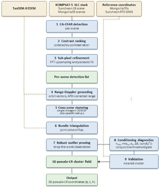
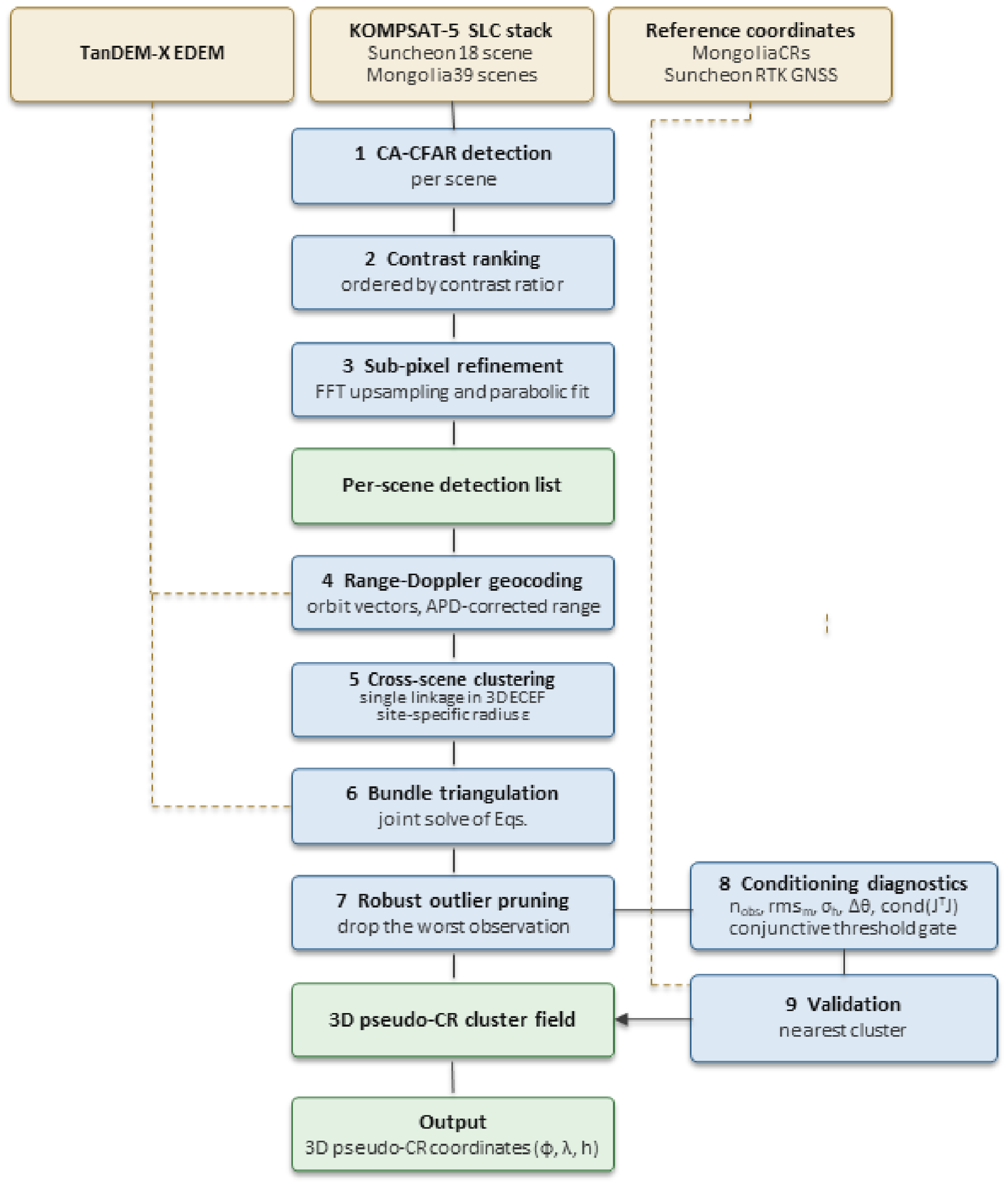
Figure 1 summarises the processing chain, the governing quantities of each stage and the intermediate products that connect them. Stages 1–3 operate on one scene at a time and produce a per-scene list of point-like candidates; stages 4–7 combine the candidates of all scenes of a stack into 3D pseudo-CR clusters; stages 8–9 attach a conditioning diagnostic vector to every cluster and evaluate the result against reference coordinates. The stage parameters and their provenance are described in Section 3.2, Section 3.3, Section 3.4 and Section 3.5 and Appendix A.

Figure 1. Overall processing flow of the proposed pseudo-CR detection and 3D positioning pipeline and the intermediate products that connect them. Solid arrows carry image or coordinate products; dashed lines carry auxiliary data. Reference coordinates enter only at the validation stage and are never used to form or select clusters.

3.1. Study Sites and Datasets

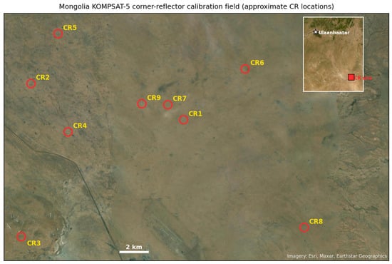
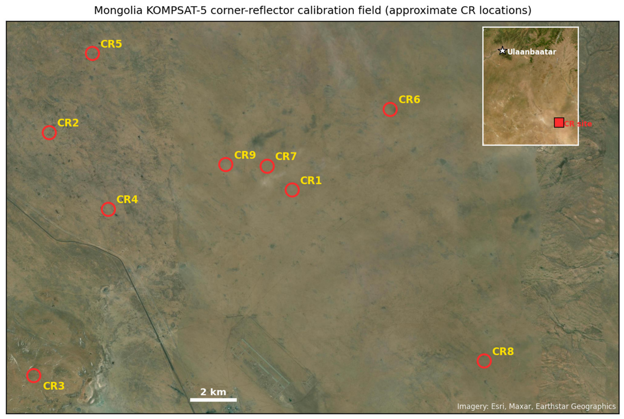
Two study sites were used. The Mongolia calibration site (centred near 46.65°N, 108.30°E) is a high-altitude steppe area operated by KARI for KOMPSAT-5 calibration and validation; it contains a set of maintained trihedral CRs, nine of which fall within the footprint of the 2024 scene stack used here and were surveyed by GNSS to centimetre accuracy. Their approximate locations are shown in Figure 2. We used 39 K5 standard-mode SLC scenes acquired during 2024 over this site, processing all scenes through the proposed pipeline.

Figure 2. Approximate locations of the nine GNSS-surveyed KOMPSAT-5 corner reflectors (CR1–CR9) in the KARI calibration field southeast of Ulaanbaatar, Mongolia, shown on satellite imagery; the inset locates the field relative to Ulaanbaatar. Marker positions are approximate. CR identifiers correspond to the GCP IDs.

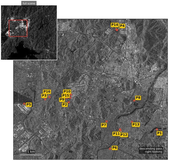
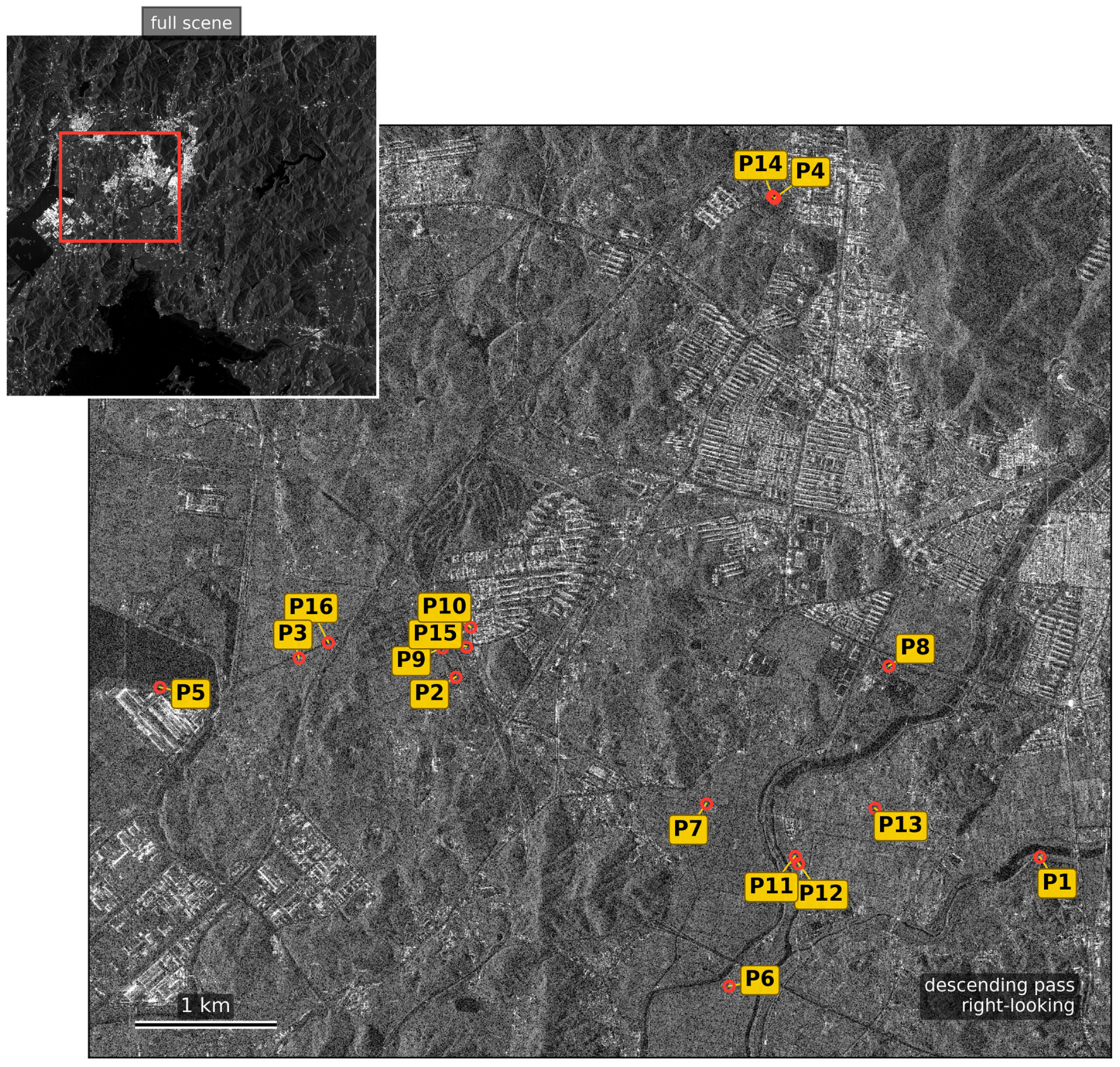
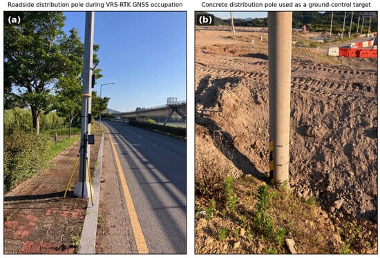
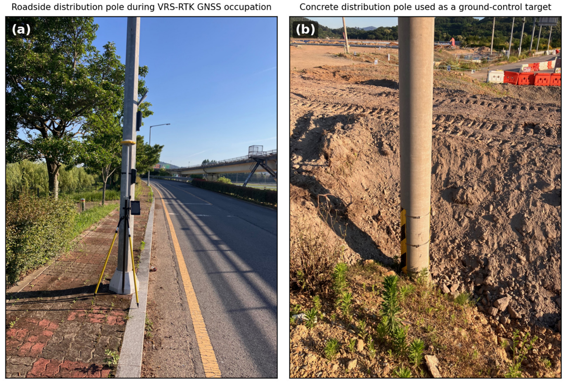
The Suncheon study site (~127.5°E, 34.95°N, Republic of Korea) is a suburban-rural area with no CRs. Seventeen K5 standard-mode SLC scenes and one Enhanced High-Resolution (EH) scene acquired between December 2022 and September 2024 (Table 1) were processed. The single EH scene covers only the central part of the site and contributed observations to 2 of the 16 pole clusters (Figure 3), so the mixed-resolution aspect is demonstrative rather than central to the validation. The reference targets are free-standing electric distribution poles (approximately 30 cm diameter) surveyed with VRS-network RTK GNSS (Figure 4); none are roof-mounted or building-attached, and all are occupied at the pole base.

Table 1. Suncheon SLC stack summary.

Stack Component	Scenes	Orbit Coverage	Approximate Pixel Spacing/Resolution
K5 standard-mode SLC	17	ascending and descending	~0.8–1.6 m range spacing; ~1.8–2.0 m azimuth spacing
K5 Enhanced High-Resolution (EH) SLC	1	ascending	~1 m ground-range and azimuth resolution

Figure 3. KOMPSAT-5 SAR amplitude of the Suncheon test region (descending ES14 scene, 7 December 2022), read from the single-look complex product at one-third sampling and displayed in decibels, with the 16 GNSS-surveyed evaluation poles (P1–P16) marked by circles and labelled through leader lines so that every identifier remains legible. The inset shows the full scene with the extent of the test region outlined in red.

Figure 4. Representative Suncheon ground-control targets: (a) a roadside electric distribution pole during VRS-network RTK GNSS occupation; (b) a free-standing concrete distribution pole used as a ground-control target.

The Suncheon survey was assembled in two phases. Initial poles were surveyed before SAR processing; because most did not yield usable multi-scene responses, additional poles were surveyed near pipeline-derived positions, with a few nearby poles added where association was ambiguous. Forty-one poles were surveyed, and 16 that formed stable responses, produced clusters meeting Section 3.5 criteria and were selected by author adjudication constitute the evaluation set. Consequently, the Suncheon results are conditional on response formation and retention and do not estimate detection probability over arbitrary poles.

Pole presence at each retained location was cross-checked against 25 cm NGII orthophoto imagery. This confirms a pole at the surveyed coordinate but is not an independent interpretation and does not identify the SAR scatterer. Retention was adjudicated on the pre-correction field and recorded only as a retained/excluded flag. The reported association is then formed automatically by taking the nearest conditioning-filtered cluster to each retained pole; it is a positional difference, not an author-verified pole-to-cluster identity.

The surveyed coordinate is the centimetre-accurate pole base, whereas the dominant radar return may arise from a crossarm, insulator, transformer or adjacent wire. The vertical differences therefore combine positioning error with this reference-point mismatch and are not treated as pure height errors.

Topographic information was provided by the TanDEM-X 30 m EDEM (1-arcsecond posting), using the TDM1_EDEM_10_N34_35E127 mosaic for Suncheon and the TDM1_EDEM_10_N46E108 tile for Mongolia, in WGS84 ellipsoidal heights. The TanDEM-X mission and global DEM accuracy assessment are described in [24,25].

3.2. Detection of Point Scatterer Candidates

3.2.1. CFAR Detection with Local Contrast Ranking

Each SLC is converted to power and processed by cell-averaging CFAR (CA-CFAR). Both production catalogues used a square pixel training window with a guard band; the metric-window option evaluated in Section 4.4.2 converts physical dimensions separately using the recorded range and azimuth spacings. For pixel x, the local contrast ratio is

$$r(x,y)={\displaystyle \frac{I_p(x,y)}{{\hat{\mu }}_n(x,y)}}$$

(1)

in which the denominator is the local clutter power, estimated by integral-image subtraction of the guard region from the training region. Equation (1) is a contrast ratio and not by itself a detection rule. Under the usual assumption that the clutter power is exponentially distributed with an unknown local mean, the cell-averaging estimate leads to the decision rule

$$r(x,y)>\alpha ,\alpha =-\mathrm{l}\mathrm{n}{P}_{fa}$$

(2)

A candidate is declared when r(x) > alpha. The production detector uses alpha = −ln(P_fa), the large-N form used to generate both catalogues (P_fa = 5 × 10⁻⁵ for Mongolia and 0.2 for the permissive Suncheon run). The finite-sample CA multiplier is used only in the controlled comparison of Section 4.4.2, where detector thresholds are ultimately matched by measured background exceedance density.

Candidates are ranked by descending local contrast rather than absolute power. Section 4.4.1 evaluates this choice at equal per-scene candidate budgets.

3.2.2. Multi-Scale Shape Templates with Size and Area Gates

Each candidate is scored against a bank of normalised templates representing the canonical impulse-response shapes of point, plus and cross scatterers at several scales. The scales are specified either in pixels or in metres and converted per scene; the Mongolia run used a single analysis scale, while the permissive Suncheon run used several smaller scales together with line templates, so that both compact and slightly elongated responses are scored. For each candidate, the winning template type and scale are recorded as (shape, template_size, tpl_score). Two further geometric gates may be applied to enforce a point-like response:

• Linear bounding-box size: the half-power (≥0.5 × peak) mask must have maximum row or column extent ≤ point_extent.
• Bright-pixel area: the count of pixels above the 0.5 × peak threshold must lie between point_area_min and point_area_max.

Both gates are specified either in pixels or in m² (with automatic per-scene conversion using range_spacing × azimuth_spacing). The area gate rejects compact-but-large blobs that pass the linear extent test. The gates are optional, and the two runs reported here use them differently: the Mongolia run applies an extent limit, whereas the permissive Suncheon run leaves both gates open so that weak and slightly elongated pole responses are retained for the triangulation stage, where the cross-scene consistency requirement takes over the role of rejecting non-point-like scatterers.

3.2.3. Sub-Pixel Refinement

Each accepted candidate is refined by two sub-pixel estimators computed from the same amplitude patch and the same discrete peak: the peak of an FFT zero-padded upsampling of the patch and a parabolic fit to the 3 × 3 neighbourhood of the discrete peak. The two estimates are averaged. Because both read the same data, they are correlated, and the average is a heuristic inherited from the implementation rather than an estimator shown here to be optimal.

For an n × n patch, the zero-padded FFT grid is referenced to the original centre (n − 1)/2. An n/2 origin shifts the FFT estimate by −0.5 pixel and the averaged estimate by −0.25 pixel; all catalogues and results reported here use the corrected convention. Their mean disagreement over 913 Suncheon detections is 0.13 pixels (99th percentile 1.5 pixels), and the Mongolia ablation in Section 4.4.7 compares them against absolute truth. On the native patch, the detector also computes a core-to-outer energy ratio, 10 log10(core/outer), using the central 3 × 3 core and pixels outside the 9 × 9 neighbourhood, with 10⁻¹² added to the denominator. This fixed-mask quantity is not conventional PSLR. A candidate is accepted when the ratio is at least a site-specific limit in decibels, larger values indicating greater core concentration, and when a normalised cross-correlation (NCC) template score in [−1, 1] is at least a site-specific limit. The Mongolia limits are the stricter pair.

3.3. Range-Doppler Geocoding

The accepted candidate’s image coordinates (x_pix, y_pix) are geocoded to WGS84 (phi, lambda, h) by inverse range-Doppler intersection. For each scene, the state vectors are interpolated from the H5 orbit table, and the observed slant range r_close is corrected for the atmospheric propagation delay (APD) provided in the H5 metadata, where c is the speed of light, and Delta_APD is the two-way delay:

$$r_{geom}=r_{close}-{\displaystyle \frac{{\Delta }_{APD}c}{2}}$$

(3)

Geocoding uses a step-clipped Gauss-Newton update of latitude, longitude and height, initialised from the DEM and including a soft DEM prior of weight 0.1. Updates are clipped component-wise, and the iteration is capped; a metre-level component tolerance is an early-stop criterion, not an acceptance criterion. The height is then reset to the DEM surface before reprojection. Solutions with residual ≤1 pixel are accepted; otherwise, an RPC inverse-location fallback is accepted under the same limit.

3.4. Multi-Look Bundle Triangulation

Per-scene detections are grouped by single-linkage clustering of their geocoded ECEF positions. The applied Suncheon radius was 15 m (50 m for Mongolia), with duplicate scene observations resolved by retaining the highest-amplitude detection. Clusters require at least three observations for Suncheon and two for Mongolia. Each cluster is jointly inverted for one ECEF point satisfying the range and zero-Doppler conditions of all member observations:

$$f_{r,k}(X)=\Vert X-S_k\left(t_k\right)\Vert -{\rho }_k=0$$

(4)

$$f_{d,k}(X)={\displaystyle \frac{\left(X-S_k\left(t_k\right)\right)·V_k\left(t_k\right)}{\Vert V_k\left(t_k\right)\Vert }}=0$$

(5)

Here X is the ground point, S_k and V_k are the satellite position and velocity at zero-Doppler time, and rho_k is the APD-corrected slant range. The residual vector contains the range and zero-Doppler residuals in metres plus the soft prior w(h_DEM − h). A Huber-weighted Levenberg–Marquardt proposal (delta = 1 m) is formed from this system. The implementation accepts or rejects proposals using the unweighted RD residual norm without the prior, so it is not a strict descent method for the full robust objective. Section 4.4.4 evaluates the DEM weight.

After each solve, the observation with the largest RD residual norm is removed when it exceeds a limit formed from an absolute floor and a multiple of the cluster median residual norm, and the cluster is re-solved for a bounded number of rounds without reducing the solution below three retained observations. This is median-scaled residual pruning, not median absolute deviation pruning.

3.5. Intrinsic Per-Target Conditioning Diagnostics

Each pruned solution receives the five conditioning diagnostics in Table 2. The reported covariance C = sigma²(J_RD^T J_RD)⁻¹ uses the unweighted RD Jacobian and excludes both Huber weights and the DEM-prior row; sigma_h is therefore an approximate geometric conditioning measure, not the propagated covariance of the robust estimator. Observation count, residual RMS, look-angle spread and cond(J_RD^T J_RD) provide complementary descriptors of redundancy, fit and geometry.

Table 2. Intrinsic per-target conditioning diagnostics.

Symbol	Definition	Selected Conditioning Threshold
n_obs	observations remaining after pruning	≥3 (≥4 preferred)
rms_m	RMS range-Doppler residual after the solve, m	≤2 m (≤4 m in the permissive Suncheon run)
sigma_h	propagated 1-sigma height uncertainty, m	≤5–10 m (≤30 m in the ascending-dominant Suncheon stack)
delta_theta	spread of the observing look angles, deg	≥10 deg preferred; ≥3 deg enforced at Suncheon
cond(JTJ)	condition number of the normal equation matrix	monitored, not thresholded (redundant with delta_theta, Section 4.4.5)

The selected gate is conjunctive: n_obs ≥ n_min, rms_m ≤ rms_max, sigma_h ≤ sigma_max and look-angle spread ≥ delta_min. The condition number is monitored but not thresholded. Applied values are given in Table 2 and evaluated in Section 4.4.5.

These are conditioning thresholds rather than a certificate of accuracy; their sensitivity and redundancy are evaluated in Section 4.2.6 and Section 4.4.5.

3.6. Validation Methodology

Each reference point is paired with the nearest triangulated cluster within R = 3, 5, 10 or 20 m by Haversine distance. The matched horizontal distance is an error for Mongolia CRs and a difference from the surveyed pole base for Suncheon; the vertical difference is relative to the ellipsoidal reference height. Counts use maximum one-to-one assignment. Mongolia provides absolute truth, whereas Suncheon statistics are conditional on the response-enriched set of Section 3.1 and do not measure recovery over all surveyed poles.

4. Results

4.1. Mongolia Calibration Site—Absolute Accuracy Benchmark

Table 3 summarises the corrected triangulation results for the nine surveyed Mongolia CRs. After residual-based pruning, all nine are positioned within 2.5 m horizontally; mean horizontal and 3D errors are 1.37 m and 2.01 m, respectively, consistent with previous KOMPSAT-5 calibration assessments [26,27].

Table 3. Mongolia CR validation results (after pruning).

GCP	n_obs	sigma_h (m)	Horiz err (m)	Height err (m)	3D err (m)
CR1	8	2.06	1.69	−2.19	2.76
CR2	10	1.52	0.95	−2.59	2.76
CR3	5	1.54	1.75	+0.36	1.79
CR4	8	1.28	0.81	+0.24	0.85
CR5	7	1.36	0.60	+0.32	0.68
CR6	5	1.25	1.65	−1.97	2.57
CR7	8	0.82	1.88	−2.07	2.80
CR8	6	1.46	0.96	−0.43	1.06
CR9	8	0.81	2.01	−2.05	2.87
Mean	7.2	1.34	1.37	−1.15	2.01

The 0.7–2.9 m 3D-error range establishes an absolute-truth benchmark for high-RCS calibration targets. It does not by itself establish equivalent accuracy for natural urban scatterers.

Table 3 sigma_h values average 1.34 m but do not order the CRs by accuracy, consistent with their interpretation as unweighted conditioning diagnostics rather than propagated robust covariances.

4.2. Suncheon Detection—Pole-Truth Validation

4.2.1. Single-Scene Detection Statistics

The permissive Suncheon run used P_fa = 0.2, a pixel-scale CFAR window, relaxed core-to-outer and NCC limits, and no size/area gate. It produced 450,652 single-scene detections over 18 scenes (Table 4); the list is intentionally clutter-rich and becomes useful only after multi-scene triangulation and conditioning-based filtering.

Table 4. Single-scene detections for the Suncheon stack under the permissive candidate-generation configuration.

Date	Mode	Orbit	Look	Detections
7 December 2022	SCS_B	D	ES14	27,801
29 June 2023	SCS_B	A	ES01	23,961
6 July 2023	SCS_B	A	ES07	20,590
13 September 2023	SCS_B	D	ES14	24,762
17 October 2023	SCS_B	A	ES06	17,617
9 November 2023	SCS_B	D	ES17	21,541
10 November 2023	SCS_B	A	ES18	29,463
11 November 2023	SCS_B	A	ES15	29,249
7 December 2023	SCS_B	D	ES17	26,799
9 December 2023	SCS_B	A	ES15	32,014
14 December 2023	SCS_B	A	ES01	23,551
9 January 2024	SCS_B	A	ES06	21,322
10 January 2024	SCS_B	A	ES04	28,143
11 January 2024	SCS_B	A	ES01	21,144
23 July 2024	SCS_B	A	ES06	23,628
10 August 2024	SCS_B	D	ES02	34,500
22 August 2024	SCS_B	A	ES01	24,519
13 September 2024	EH	A	EH30	20,048

4.2.2. Cluster Triangulation and Nearest-Cluster Positional Agreement

Triangulation produced 39,822 clusters, of which 26,659 passed rms_m ≤ 4.0 m, look-angle spread ≥ 3 degrees, sigma_h ≤ 30 m and n_obs ≥ 3. The filters reduce the field by 33.1%; Section 4.4.5 evaluates their effect.

The nearest conditioning-filtered cluster lies within 3, 5, and 10 m for 9, 14, and all 16 retained poles, respectively (Table 5). The mean horizontal difference is 3.19 m (maximum 6.14 m), and the mean absolute vertical difference from the pole base is 1.45 m. These are proximity statistics for the selected set, not verified identities or population recovery rates.

Table 5. Cumulative horizontal nearest-cluster agreement over the 16 Suncheon evaluation poles. These are conditional nearest-cluster differences on targets that produced a stable multi-scene response and were retained by author adjudication (Section 3.1); they are not a detection rate and do not estimate performance over an arbitrary pole population.

Radius (m)	Hits	Total	Fraction	Mean Horiz err (m)	Max Horiz err (m)
3	9	16	0.56	2.16	2.90
5	14	16	0.88	2.77	4.54
10	16	16	1.00	3.19	6.14
20	16	16	1.00	3.19	6.14

At the pole-region cluster density, a uniform Poisson model gives chance proximity probabilities of 0.2%, 0.6%, 2.4% and 9.3% at 3, 5, 10, and 20 m. Because the evaluation set was response-informed and author-retained, this describes unconditional scene density only and does not bound the false-association probability of the 16 reported pairs.

4.2.3. Per-Pole Geometry and Conditioning Diagnostics

Table 6 reports per-pole metrics for the 16 pole targets, all of which were matched within 10 m. The nearest clusters are typically built from 3 to 6 observations with RD residual RMS values ranging from below one metre to a few metres, and 9 of the 16 lie within 3 m. The remaining targets, with differences of 3.1–6.1 m, are examined below against the geometry and scattering diagnostics; detector and association error remain possible contributors that these data cannot separate.

Table 6. Nearest-cluster differences and intrinsic conditioning diagnostics for the 16 response-enriched, retained Suncheon poles, including the signed vertical difference relative to the surveyed pole base. Each row pairs a surveyed pole with the conditioning-filtered cluster nearest to it, which is a proximity measurement and not a verified identification of the scatterer. The label column gives the original GNSS survey identifier; the P1–P16 aliases were assigned in ascending order of the pre-correction horizontal error and are retained only so that the discussion can refer to individual targets. They are not a physical ordering, and after the sub-pixel correction of Section 4.4.7, the error ranking no longer follows the alias order.

Survey ID (Alias)	Horiz err (m)	n_obs	rms_m	Spread (deg)	sigma_h (m)	Vert diff (m)
Survey 23 (P1)	1.50	4	2.21	27.4	5.11	+0.31
Survey 41 (P5)	1.59	4	0.90	103.9	1.06	−1.71
Survey 34 (P3)	1.65	3	0.50	84.4	0.55	−1.89
Survey 38 (P4)	1.87	4	0.63	19.7	2.23	−1.10
Survey 26 (P7)	2.25	4	1.69	99.7	1.54	−0.45
Survey 39 (P8)	2.39	6	0.87	100.0	0.61	−1.65
Survey 40 (P6)	2.47	4	0.62	71.1	0.66	−1.29
Survey 32 (P10)	2.82	6	0.63	33.3	0.90	+0.02
Survey 28 (P9)	2.90	4	0.86	103.9	1.02	−2.17
Survey 25 (P11)	3.06	6	0.66	26.1	1.22	−0.01
Survey 24 (P12)	3.82	3	0.68	20.0	2.25	+0.44
Survey 15 (P13)	3.90	4	0.36	13.9	1.14	+0.70
Survey 37 (P14)	4.07	3	0.57	33.7	1.19	+0.65
Survey 27 (P2)	4.54	4	0.57	23.2	1.51	+4.71
Survey 33 (P16)	6.01	3	0.60	4.1	11.65	+2.28
Survey 31 (P15)	6.14	5	1.33	33.7	1.81	+3.84

The diagnostics support three candidate mechanisms without identifying their causal shares: weak geometry for clusters with few looks or narrow angular spread; association ambiguity where several tall scatterers occur nearby; and reference-point offset between the surveyed pole base and the dominant response on the structure. Table 7 applies the explicit priority rule below as a post hoc diagnostic grouping.

Table 7. Error-source grouping of the 16 Suncheon evaluation poles. Groups are assigned by the priority rule described in the text and are mutually exclusive.

Group	Members	n	Mean Horizontal Difference (m)	Median Horizontal Difference (m)	Mean Absolute Vertical Difference (m)	Mean sigma_h (m)	Mean Look-Angle Spread (deg)
G1 weak acquisition geometry	P1, P13, P16	3	3.80	3.90	1.10	5.96	15.1
G2 crowded vertical scatterers	P4, P11, P12, P14	4	3.21	3.44	0.55	1.72	24.9
G3 residual stratum (scattering-centre offset hypothesised)	P5, P3, P7, P8, P6, P10, P9, P2, P15	9	2.97	2.47	1.97	1.07	72.6
All evaluation targets	P1–P16	16	3.19	2.86	1.45	2.15	49.9

4.2.4. Error-Source Grouping of the Evaluation Poles

Each pole is assigned once by priority: G1 for look-angle spread < 15 degrees or sigma_h > 3 m; otherwise G2 when another surveyed pole is within 100 m; otherwise G3. G1/G2/G3 contain 3, 4 and 9 poles. Kruskal–Wallis tests find no significant group difference in horizontal (H = 0.48, p = 0.79) or absolute vertical difference (H = 3.85, p = 0.15). Because grouping uses survey information and G3 is residual, it is diagnostic rather than a ground-truth-free error classifier or quantitative error budget.

4.2.5. What the Evaluation Set Can and Cannot Support, and Persistence of the Retained Field

Because the second survey phase used pipeline-derived positions, no recovery rate over all 41 poles is reported. The 16-target statistics quantify nearest-cluster agreement only after a stable response formed and was retained; this selection favours easier targets and is plausibly optimistic.

A leave-scene-out diagnostic tested 300 sampled clusters and 300 random positions in scenes excluded from the corresponding solutions. Of 254 evaluable clusters, 85.8% showed a peak at least 10 dB above background, versus 35.2% of 270 evaluable controls. Their background-normalised persistence enrichment is 78% (95% bootstrap interval 71–85%); missing-outcome sensitivity gives 53–82% under adverse cross-arm imputation. This demonstrates greater held-out-scene persistence, not point-target shape, object identity or catalogue precision. Controls were unmatched on land cover and scene availability, and no independent interpreter assessed candidates. The independent precision assessment therefore remains outstanding. It would require a random candidate sample, suitable reference imagery and two interpreters uninvolved in this work; Section 5.5 summarises the required design.

A second diagnostic addresses local membership ambiguity rather than brightness or identity. For a fixed-seed random sample of 1500 entries that passed the conditioning gate, the unmodified solutions for all entries were recomputed and passed the gate, confirming faithful reconstruction of the archived solutions. We then searched the archived triangulation-member table for other detections from the same contributing scenes within 25 m. Thirty-seven entries (2.5%) had alternatives in at least three contributing scenes. Five fixed-seed local replacement groupings were generated for each of these entries and processed through the same triangulation, pruning, and conditioning-gate pipeline; 122 of 185 replacement groupings (66%) passed. Because the five draws from each entry are correlated, this fraction is descriptive, and no binomial confidence interval is assigned. The result shows that the gate often does not resolve membership ambiguity when archived local alternatives exist. The test is conditioned on an already retained entry and uses only detections represented in the archived membership table; it therefore estimates neither catalogue precision nor the frequency of chance co-location and does not establish physical identity. Independent reference interpretation remains necessary.

4.2.6. Conditioning Diagnostics Versus Absolute Error

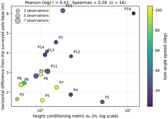
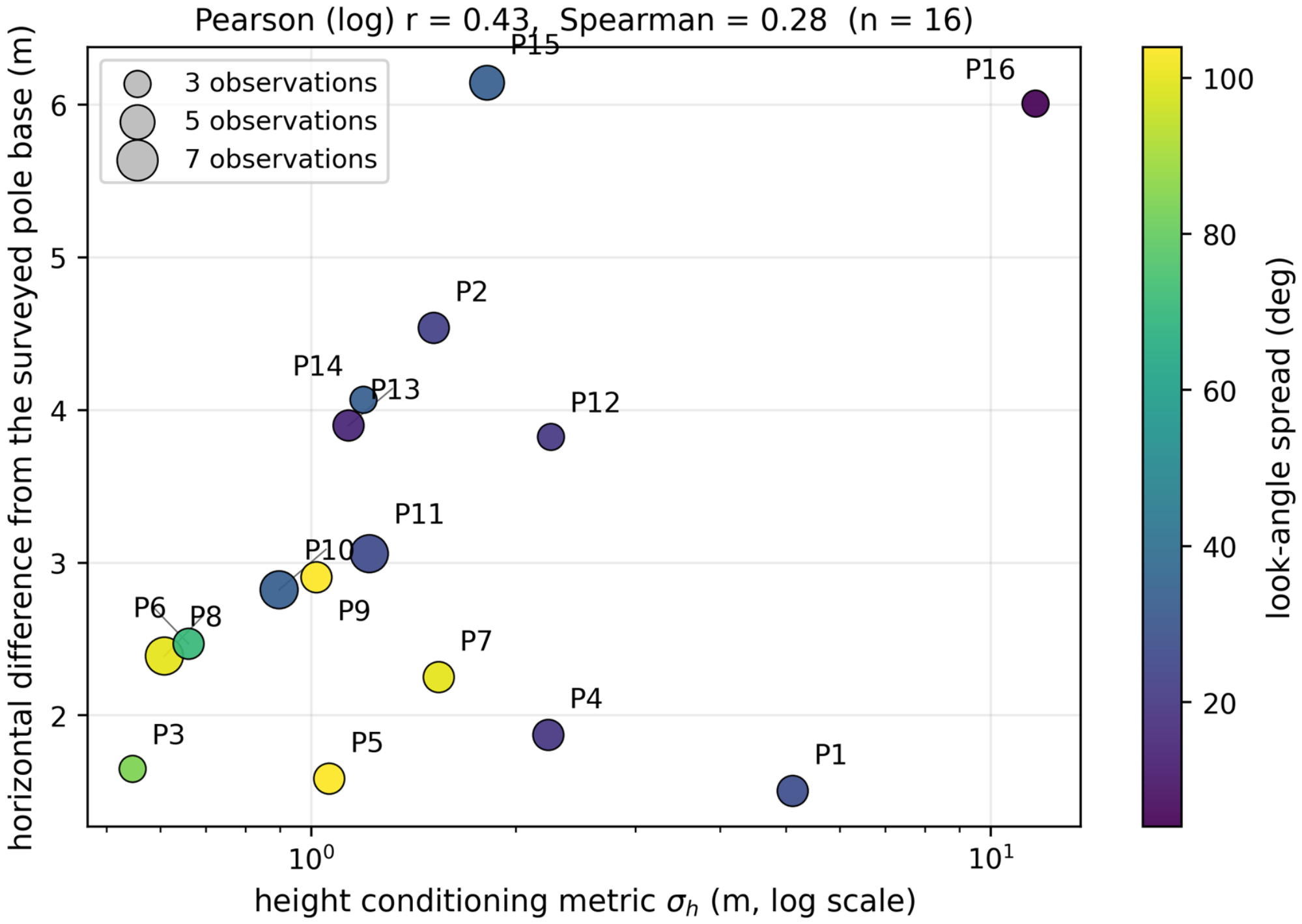
Figure 5 shows that sigma_h identifies the clearly weak-geometry case P16 but provides little ordering among the remaining targets. Its Pearson/Spearman correlations with horizontal difference are 0.43/0.28, compared with 0.59/0.46 for condition number and −0.55/−0.44 for look-angle spread. None is sufficiently predictive to infer target accuracy; the vector is used to describe conditioning and flags weak geometry.

Figure 5. Height conditioning metric sigma_h versus the horizontal difference from the surveyed pole base for the 16 Suncheon evaluation poles, coloured by look-angle spread and sized by the number of contributing observations. Labels displaced from their markers are connected to them by leader lines. sigma_h is the unweighted geometric conditioning metric defined in Section 3.5, not the propagated covariance of the robust estimator. The poorly constrained narrow-geometry cluster P16 (4.1-degree spread, sigma_h = 11.7 m) is flagged clearly, but among the well-conditioned clusters the diagnostic carries little ordering information (Pearson r = 0.43 on the log-transformed diagnostic, Spearman r = 0.28), which is why it is used to exclude clearly weak conditioning rather than to predict accuracy.

4.3. Look-Direction Visibility and Orbit Dependence

The 16 clusters contain 68 observations: 43 ascending and 25 descending. Thirteen targets are ascending-dominant, two descending-dominant, and one balanced, but target-level horizontal difference is not significantly related to that classification (p = 0.69). Visibility is thus target-specific, while the ascending-dominant stack limits geometric diversity overall.

4.4. Ablation and Parameter Sensitivity

The experiments in this section examine the effects of selected pipeline elements. All runs reuse the detection lists, reference coordinates, and matching procedure from Section 4.1 and Section 4.2, so within each comparison the only difference is the component or parameter under test.

4.4.1. Ranking Criterion: Absolute Power Versus Local Contrast

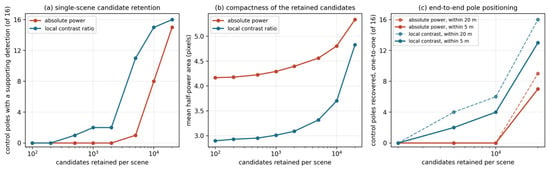
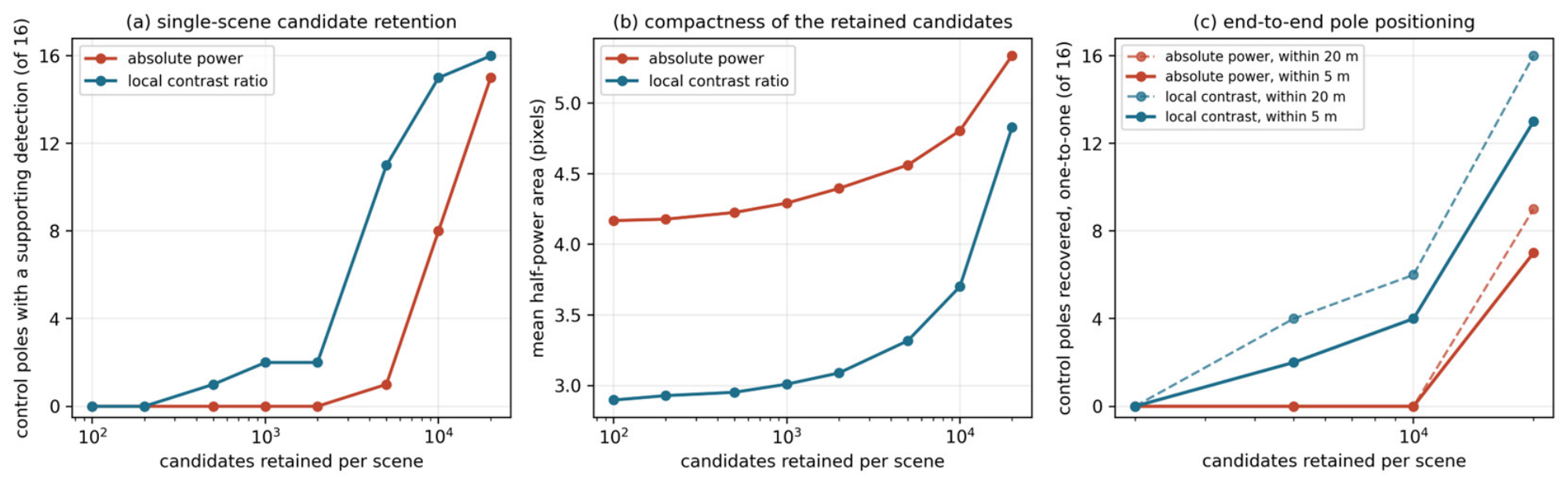
Absolute-power and local-contrast rankings were compared using identical detections and equal per-scene candidate budgets. Contrast ranking retains weak point-like responses that power ranking places below bright extended clutter; at the full budget it retains all 16 evaluation targets versus 9 for power ranking (Table 8 and Figure 6).

Table 8. End-to-end effect of the ranking criterion. Both arms use the same detections, the same triangulation chain and the same matching procedure, and differ only in which candidates survive the per-scene budget.

Candidates per Scene	Ranking Criterion	Clusters	Within 3 m	Within 5 m	Within 10 m	Within 20 m	Mean Horizontal Difference Within 20 m (m)
2000	absolute power (conventional)	2932	0/16	0/16	0/16	0/16	-
2000	local contrast (proposed)	2447	0/16	0/16	0/16	0/16	-
5000	absolute power (conventional)	8183	0/16	0/16	0/16	0/16	-
5000	local contrast (proposed)	7591	2/16	2/16	3/16	4/16	7.08
10,000	absolute power (conventional)	16,857	0/16	0/16	0/16	0/16	-
10,000	local contrast (proposed)	17,694	3/16	4/16	5/16	6/16	5.49
20,000	absolute power (conventional)	32,624	3/16	7/16	9/16	9/16	4.32
20,000	local contrast (proposed)	34,471	8/16	13/16	16/16	16/16	3.55
all (~25,000)	local contrast (Section 4.2.2)	39,822	9/16	14/16	16/16	16/16	3.19

Figure 6. Effect of the candidate ranking criterion, evaluated over the 16 Suncheon evaluation targets. (a) Number of targets that keep at least one supporting detection within 20 m when each per-scene detection list is truncated to the top N candidates. (b) Mean half-power area of the retained candidates, a proxy for how point-like the retained population is. (c) Number of evaluation targets positioned within 5 m and within 20 m, under maximum one-to-one assignment, after the truncated lists are pushed through the complete triangulation chain.

The truncated lists were passed through the same geocoding, triangulation, pruning and one-to-one matching chain. Contrast ranking reaches 16 targets within 20 m, whereas power ranking reaches 9 at the same full budget.

This is an exploratory conditional ablation: the evaluation set is response-enriched and was partly selected from contrast-based preliminary output. The experiment therefore measures the ranking effect on this set, not blind population recall or catalogue precision.

4.4.2. Comparison with Conventional CFAR Variants

CA, greatest-of (GO), smallest-of (SO) and 75th-percentile ordered-statistic (OS) CFAR were compared on 86 common valid scene-pole patches from six scenes. Each used identical power data and was evaluated with isotropic pixel and metric-anisotropic windows. Border pixels were excluded for all variants, and thresholds were selected from pooled background-ratio quantiles to match the realised exceedance density within 0.33%. A hit is a threshold crossing within five pixels of the predicted pole position, not identification of the pole.

Across all eight operating points, CA and GO exceed SO and OS, while SO and OS exchange order. GO point estimates equal or exceed CA, but paired intervals include zero, so CA superiority is not established. Metric and isotropic windows differ by at most 2.3 percentage points, showing no consistent anisotropic-window advantage. The clearest separation is instead the ranking criterion: median pole-peak ranks at a matched density of 10⁻² are 262 by power, 91 by CA contrast and 90 by GO contrast (Table 9).

Table 9. Proximity-hit rate on the surveyed poles at matched background exceedance density, and the median rank of the pole peak among the background pixels of the same patch, for four reference-window detectors and two window definitions (six scenes, 86 valid scene-pole patches over the 16 evaluation targets). A hit means a threshold crossing within five pixels of the predicted pole position, which is a proximity test rather than identification of the pole. All variants are scored on the common valid interior of each patch, where every reference window is fully contained, and each column is read at the quantile of that variant’s own pooled background ratios that realises the stated density. The exceedance count above the threshold is measured, not assumed, so ties leave every column within 0.33% of its nominal target.

Training Window	Detector	Proximity-Hit Rate at Background Exceedance Density 10−2	at 3 × 10−3	at 10−3	at 3 × 10−4	Median Rank of the Pole Peak, Power Ordering	Median Rank of the Pole Peak, Contrast Ordering
isotropic pixel	CA	68.6%	38.4%	26.7%	15.1%	262	105
isotropic pixel	GO	68.6%	41.9%	29.1%	15.1%	262	108
isotropic pixel	SO	57.0%	31.4%	18.6%	8.1%	262	216
isotropic pixel	OS	55.8%	32.6%	16.3%	7.0%	262	152
metric 40 m (anisotropic)	CA	68.6%	40.7%	26.7%	15.1%	262	91
metric 40 m (anisotropic)	GO	69.8%	40.7%	29.1%	16.3%	262	90
metric 40 m (anisotropic)	SO	55.8%	33.7%	17.4%	9.3%	262	172
metric 40 m (anisotropic)	OS	61.6%	34.9%	18.6%	8.1%	262	122

4.4.3. Pipeline-Component Ablation on the Mongolia Corner Reflectors

Table 10 re-runs the complete Mongolia triangulation while changing one component at a time. Removing pruning alone increases the mean 3D error from 2.01 m to 2.97 m and reduces the count within 2.5 m horizontally from 9/9 to 4/9; removing Huber weighting alone increases the mean 3D error to 4.84 m with 7 of 9 within 2.5 m; removing both gives 7.39 m and 2 of 9. Huber weighting therefore has the larger effect on the mean 3D error in this experiment, while pruning has the larger effect on the number of reflectors recovered within 2.5 m. Both are needed, and neither alone accounts for the robust configuration’s advantage.

Table 10. Component ablation and parameter variation on the nine Mongolia corner reflectors. Every row re-runs the complete triangulation with one element removed or one parameter changed and re-matches the result against the surveyed coordinates.

Configuration	Clusters	CRs Within 2.5 m Horizontally	Mean Horizontal Error (m)	RMS Horizontal Error (m)	Mean 3D Error (m)	Max 3D Error (m)	Mean Signed Height Error (m)	Mean sigma_h (m)
Full pipeline (Huber + pruning, DEM weight 0.10)	97	9/9	1.37	1.46	2.01	2.87	−1.15	1.34
without iterative outlier pruning	97	4/9	2.38	2.65	2.97	4.28	+0.34	5.57
without Huber weighting	97	7/9	3.27	4.88	4.84	16.72	+0.83	3.05
without either (plain least squares)	97	2/9	5.61	6.45	7.39	16.72	+3.94	5.33
without the DEM soft prior (weight 0)	97	9/9	1.39	1.48	2.05	2.92	−1.16	1.34
DEM weight 0.02	97	9/9	1.38	1.48	2.05	2.92	−1.16	1.34
DEM weight 0.05	97	9/9	1.38	1.47	2.04	2.90	−1.16	1.34
DEM weight 0.20	97	9/9	1.33	1.42	1.92	2.80	−1.14	1.35
DEM weight 0.50	97	8/9	1.21	1.39	1.62	2.94	−1.00	1.35
DEM weight 1.00	97	7/9	1.17	1.49	1.49	3.23	−0.83	1.38
clustering minimum observations raised from 2 to 3	53	9/9	1.37	1.46	2.01	2.87	−1.15	1.34
cluster eps 25 m	102	9/9	1.37	1.46	2.01	2.87	−1.15	1.34
cluster eps 75 m	96	9/9	1.37	1.46	2.01	2.87	−1.15	1.34
cluster eps 100 m	92	9/9	1.37	1.46	2.01	2.87	−1.15	1.34

Raising the pre-triangulation cluster-eligibility minimum from two observations to three, varying the clustering radius, and varying the DEM-prior weight over the tested low range each have little effect at the sparse Mongolia site. These findings do not evaluate atmospheric modelling or detector-induced changes in cluster membership.

4.4.4. Weight of the DEM Soft Prior

Varying the DEM weight from 0 to 0.10 changes the mean Mongolia 3D error only from 2.05 m to 2.01 m. Larger weights lower the mean by pulling solutions toward the DEM but displace targets: 0.50 retains 8/9, and 1.00 retains 7/9 within 2.5 m horizontally. The applied low weight therefore stabilises weak height geometry without making the DEM the solution.

4.4.5. Conditioning Thresholds and Diagnostic Redundancy

Table 11 varies each Suncheon conditioning threshold while holding the others fixed. Moderate changes leave all 16 evaluation targets positioned within 20 m, whereas strict limits reduce the field and lose targets. Removing the gate adds 13,163 clusters but no evaluation targets, showing that the applied gate reduces catalogue size without improving or degrading the conditional count.

Table 11. Sensitivity of the retained cluster field, and of how many evaluation targets are positioned within each radius, to each conditioning threshold; the remaining thresholds are held at the applied values (rms 4 m, spread 3 degrees, height conditioning metric 30 m, three observations). The counts are evaluation targets positioned within each radius under a maximum one-to-one assignment over the 16 retained evaluation poles; they are conditional positioning counts, not recall estimates. The lower block gives joint operating points.

Threshold Varied	Value	Retained Clusters	Fraction of the Field	Within 3 m	Within 5 m	Within 10 m	Within 20 m	Mean Horizontal Difference Within 20 m (m)
residual RMS limit (m)	1	9611	24.1%	7	12	13	13	3.16
residual RMS limit (m)	2	16,863	42.3%	8	13	15	15	3.30
residual RMS limit (m)	3	22,440	56.4%	9	14	16	16	3.19
residual RMS limit (m)	4	26,659	66.9%	9	14	16	16	3.19
residual RMS limit (m)	6	32,223	80.9%	9	14	16	16	3.19
residual RMS limit (m)	no limit	37,234	93.5%	9	14	16	16	3.19
minimum look-angle spread (deg)	0	26,990	67.8%	9	14	16	16	3.19
minimum look-angle spread (deg)	3	26,659	66.9%	9	14	16	16	3.19
minimum look-angle spread (deg)	5	23,843	59.9%	9	14	15	15	3.00
minimum look-angle spread (deg)	10	22,423	56.3%	9	14	15	15	3.00
minimum look-angle spread (deg)	20	20,765	52.1%	8	11	12	12	2.95
minimum look-angle spread (deg)	30	16,800	42.2%	7	8	9	9	2.92
height-uncertainty limit (m)	5	21,656	54.4%	8	13	14	14	3.10
height-uncertainty limit (m)	10	24,417	61.3%	9	14	15	15	3.00
height-uncertainty limit (m)	20	26,119	65.6%	9	14	16	16	3.19
height-uncertainty limit (m)	30	26,659	66.9%	9	14	16	16	3.19
height-uncertainty limit (m)	50	27,645	69.4%	9	14	16	16	3.19
height-uncertainty limit (m)	no limit	27,917	70.1%	9	14	16	16	3.19
minimum observations	2	26,659	66.9%	9	14	16	16	3.19
minimum observations	3	26,659	66.9%	9	14	16	16	3.19
minimum observations	4	15,672	39.4%	8	11	12	12	2.95
minimum observations	5	9266	23.3%	2	3	4	4	3.60
minimum observations	6	5716	14.4%	2	3	3	3	2.76
joint: no conditioning filter	-	39,822	100.0%	9	14	16	16	3.19
joint: applied gate (4 m, 3 deg, 30 m, 3 obs)	-	26,659	66.9%	9	14	16	16	3.19
joint: strict gate (2 m, 3 deg, 10 m, 3 obs)	-	15,072	37.8%	8	13	14	14	3.10
joint: very strict gate (2 m, 10 deg, 5 m, 4 obs)	-	8134	20.4%	7	10	11	11	3.08

Passing the gate is not a reliability certificate. P16, the worst-conditioned target, passes the applied limits; tightening sigma_h removes it, while a strict residual limit also removes P1, the best-positioned target. The diagnostics therefore describe conditioning and reject clear weakness but do not rank accuracy among survivors.

Table 12 reports diagnostic correlations over all 39,822 clusters. Look-angle spread and condition number are strongly redundant (Spearman −0.90; log-Pearson −0.86). VIFs range from 3.6 to 31.8, and the smallest eigenvalue is 0.013, while three components explain 97% of the variance. Observation count and residual RMS contribute more distinct information, supporting a conjunctive gate rather than a single composite score.

Table 12. Spearman rank correlation between the conditioning diagnostics over all 39,822 triangulated Suncheon clusters (upper value in each cell) and the Pearson correlation of the log-transformed diagnostics (lower value). The variance inflation factors and eigenvalues quoted in the text are computed from the log-transformed Pearson matrix, not from the Spearman matrix.

Diagnostic	n_obs	rms_m	sigma_h	delta_theta	cond (JTJ)	VIF (Log-Pearson)
n_obs	1.00/1.00	0.49/0.52	−0.28/−0.20	0.63/0.53	−0.52/−0.41	3.6
rms_m	0.49/0.52	1.00/1.00	0.39/0.30	0.51/0.51	−0.50/−0.44	20.0
sigma_h	−0.28/−0.20	0.39/0.30	1.00/1.00	−0.41/−0.49	0.40/0.68	25.6
delta_theta	0.63/0.53	0.51/0.51	−0.41/−0.49	1.00/1.00	−0.90/−0.86	4.9
Cond (JTJ)	−0.52/−0.41	−0.50/−0.44	0.40/0.68	−0.90/−0.86	1.00/1.00	31.8

4.4.6. Clustering Radius in the Dense Suncheon Pole Field

The clustering radius is immaterial for the widely separated Mongolia CRs but consequential in Suncheon. At 15 m, all 16 retained poles are positioned within 20 m; at 20 m, the count falls to 12, and at 30 m, to 9, as nearby structures merge through single linkage (Table 13). The applied 15 m value lies at the upper edge of the stable region and should not be transferred to denser fields without a spacing-based sensitivity check.

Table 13. Sensitivity of the Suncheon cluster field, and of how many evaluation targets lie within each radius, to the clustering radius. The counts are evaluation targets positioned within each radius under maximum one-to-one assignment over the 16 retained poles—not a recall—and the last column is their mean horizontal difference.

Clustering Radius (m)	Clusters	After Conditioning Gate	Mean Observations Per Cluster	Within 3 m	Within 5 m	Within 10 m	Within 20 m	Mean Horizontal Difference, 16 Evaluation Targets (m)
7.5	39,004	35,041	4.33	9/16	15/16	16/16	16/16	3.04
10	42,162	35,613	4.43	9/16	14/16	16/16	16/16	3.19
15 (used)	39,822	26,659	4.47	9/16	14/16	16/16	16/16	3.19
20	30,892	16,951	4.38	8/16	12/16	14/16	14/16	3.22
25	22,410	10,868	4.30	7/16	10/16	12/16	12/16	3.38
30	17,074	7565	4.24	6/16	8/16	9/16	9/16	3.21

4.4.7. Effect of the Sub-Pixel Estimator Correction

Correcting the FFT origin shifts each averaged peak by +0.25 pixel. Amplitude and phase were recomputed at the corrected locations, and 1146 edge cases whose patches could not be recovered were excluded consistently. Mongolia changes are small and mixed; in Suncheon, the mean horizontal difference rises from 2.87 m to 3.19 m because the nearest cluster changes for P2. This shows that the earlier agreement was partly sensitive to association in the dense field.

For Mongolia, mean horizontal error changes from 1.38 m to 1.37 m and mean 3D error from 2.00 m to 2.01 m; all nine CRs remain within 2.5 m horizontally. The correction therefore removes a known coordinate bias without materially changing the absolute-truth result.

A fixed-membership ablation over the nine Mongolia CRs compares FFT-only, the production mean and parabolic-only coordinates for the same 65 observations. Mean 3D errors are 1.99, 2.02 and 2.05 m, and all three retain 9/9 within 2.5 m horizontally. Paired 95% percentile-bootstrap intervals (20,000 resamples) are −66 to +14 mm for FFT minus mean and −10 to +81 mm for parabolic minus mean; both include zero. The experiment establishes neither superiority nor equivalence and does not test changes in detection or cluster membership, so the production mean is retained.

5. Discussion

5.1. The Resolution-Limited Regime

Mongolia 3D errors of 0.7–2.9 m are consistent with the mid-resolution regime and with reported GF-3 stereo results [16,17]. Centimetre-level TerraSAR-X positioning additionally relies on approximately 1 m imagery, propagation corrections, collocated GNSS and favourable geometry [8]. Within the components tested here, robust estimation has the largest effect; propagation-model refinement was not ablated and cannot be ranked against it.

5.2. Pole Detection at Mid-Resolution K5: Physical Limits

At standard-mode resolution, a pole occupies only a few pixels and its dominant response may come from attached hardware. The 3.19 m Suncheon mean therefore demonstrates few-metre nearest-cluster agreement only for the selected poles that formed stable responses. Population detection rate and catalogue precision require separate experiments; higher-resolution EH or spotlight data are expected to improve per-scene detectability but would not remove association and truth-definition limits [28,29]. Reviews of spaceborne high-resolution spotlight and sliding-spotlight imaging set out the modes that deliver such resolutions [30], and absolute 2-D and 3-D localisation measurements on TerraSAR-X give the accuracy that such modes can support under favourable conditions [31].

5.3. Conditioning Diagnostics Without Ground Control

Without CRs, the intrinsic diagnostics describe whether the viewing geometry and residuals support a solution. Sigma_h flags clear weak geometry but correlates only weakly with Suncheon horizontal difference and does not rank the survivors. It is therefore a conditioning descriptor, not a ground-truth-free accuracy predictor.

The leave-scene-out result provides internal evidence of persistence but not precision or object identity. The random controls are unmatched, the proportions are calculated from complete cases, and the test can retain stable ghost responses [28]. Independent interpretation of a random catalogue sample remains necessary.

5.4. Comparison to Related Approaches

The method addresses absolute 3D geolocation from geometrically heterogeneous, mid-resolution stacks. Table 14 distinguishes this quantity from relative line-of-sight deformation precision in PSI; millimetre-level PSI precision and metre-level absolute geolocation are not directly comparable.

Table 14. Comparison with related stereo, radargrammetric and time-series approaches. The accuracy metric differs between columns and the figures are not directly comparable: the stereo and radargrammetric columns report absolute 3D geolocation accuracy against surveyed coordinates, whereas the PSI column reports the precision of relative line-of-sight deformation along a time series, which does not constitute absolute positioning.

Property	This Work	Conventional CFAR Baseline (This Study, Section 4.4.1)	Gisinger et al. [8]	GF-3 Stereo SAR [16,17]	PSI [10,13]
Sensor	KOMPSAT-5 mid-resolution	KOMPSAT-5 mid-resolution	TerraSAR-X high-resolution spotlight	GF-3 spotlight	various
GSD	2.5–3 m (+one 1 m EH scene)	2.5–3 m	~1 m	~1 m	various
Scenes per stack	18 (Suncheon), 39 (Mongolia)	18 (Suncheon)	many	≥3	≥25
Geodynamic correction	APD only	APD only	full	partial	full
GNSS support	no collocated GNSS atmospheric correction; RTK GNSS used for validation	as in this work	collocated	none	optional
Quantity measured	absolute 3D geolocation of CRs; nearest-cluster differences from the surveyed pole base over 16 response-enriched, retained Suncheon poles (conditional, not absolute)	as this work	absolute 3D geolocation of CRs and PSs	absolute 3D geolocation	relative line-of-sight deformation (not absolute position)
Validated accuracy	0.7–2.9 m 3D for CRs (absolute); 16 Suncheon targets, mean horizontal difference 3.19 m (conditional, response-enriched set)	9 of 16 evaluation targets within 20 m at an equal candidate budget (response-enriched set; not comparable with the independently validated columns)	centimetre level	<3 m	millimetre-level deformation precision
Per-target conditioning diagnostic without GCP	yes, characterised as a conditioning descriptor (Section 5.3)	no	yes (different formulation)	partial	implicit

5.5. Limitations

The main limitation is selection: part of the Suncheon evaluation set was surveyed after processing, so its positional differences are conditional and plausibly optimistic, not a blind detection rate. Second, pole-based truth need not coincide with the radar scattering centre, especially vertically. Third, the ascending-dominant stack limits look-angle diversity. Fourth, the held-out-scene diagnostic measures recurrence of brightness, not point-target shape, physical identity or catalogue precision.

Two experiments remain distinct: a random-sample precision assessment of the existing catalogue against independent reference interpretation, and a blind detection-rate experiment using a target list fixed before processing. Both are required before operational pole-recovery claims can be made.

Generality is also limited by the two contrasting sites and by unmodelled propagation delays; thresholds should be re-evaluated for other environments and acquisition geometries.

6. Conclusions

We presented a KOMPSAT-5 pipeline combining contrast-ranked CFAR, point-like shape screening, multi-scene RD triangulation and per-target conditioning diagnostics. Controlled ablations quantify the effects of ranking, CFAR variant, robust estimation, DEM weight, conditioning thresholds, clustering radius and sub-pixel estimator.

All nine Mongolia CRs are positioned within 2.5 m horizontally, with mean horizontal and 3D errors of 1.37 m and 2.01 m. In Suncheon, 26,659 of 39,822 clusters pass the conditioning gate, and the 16 response-enriched retained poles have a mean nearest-cluster horizontal difference of 3.19 m and mean absolute vertical difference from the pole base of 1.45 m. These are conditional positional agreements, not detection probabilities or verified scatterer identities.

The diagnostics flag weak conditioning but do not predict accuracy among surviving targets. Before operational use, a blind detection-rate study and an independent catalogue-precision assessment are both required. Subject to those limitations, stable natural scatterers in limited KOMPSAT-5 stacks can provide metre-scale reference points where deployed CRs are unavailable.

References

- Doerry, A.W.; Brock, B.C. Radar Cross Section of Triangular Trihedral Reflector with Extended Bottom Plate; Sandia Report SAND2009-2993; Sandia National Laboratories: Albuquerque, NM, USA, 2009. [Google Scholar] [CrossRef] [Scilit]
- Dellinger, F.; Delon, J.; Gousseau, Y.; Michel, J.; Tupin, F. SAR-SIFT: A SIFT-like algorithm for SAR images. IEEE Trans. Geosci. Remote Sens. 2015, 53, 453–466. [Google Scholar] [CrossRef] [Scilit]
- Xiang, Y.; Wang, F.; You, H. OS-SIFT: A robust SIFT-like algorithm for high-resolution optical-to-SAR image registration in suburban areas. IEEE Trans. Geosci. Remote Sens. 2018, 56, 3078–3090. [Google Scholar] [CrossRef] [Scilit]
- Li, J.; Hu, Q.; Ai, M. RIFT: Multi-modal image matching based on radiation-variation insensitive feature transform. IEEE Trans. Image Process. 2020, 29, 3296–3310. [Google Scholar] [CrossRef] [Scilit]
- Prats, P.; Scheiber, R.; Mittermayer, J.; Meta, A.; Moreira, A. Processing of sliding spotlight and TOPS SAR data using baseband azimuth scaling. IEEE Trans. Geosci. Remote Sens. 2010, 48, 770–780. [Google Scholar] [CrossRef] [Scilit]
- Mittermayer, J.; Wollstadt, S.; Prats-Iraola, P.; Scheiber, R. The TerraSAR-X staring spotlight mode concept. IEEE Trans. Geosci. Remote Sens. 2014, 52, 3695–3706. [Google Scholar] [CrossRef]
- Prats-Iraola, P.; Scheiber, R.; Rodriguez-Cassola, M.; Mittermayer, J.; Wollstadt, S.; De Zan, F.; Braeutigam, B.; Schwerdt, M.; Reigber, A.; Moreira, A. On the processing of very high resolution spaceborne SAR data. IEEE Trans. Geosci. Remote Sens. 2014, 52, 6003–6016. [Google Scholar] [CrossRef] [Scilit]
- Gisinger, C.; Balss, U.; Pail, R.; Zhu, X.X.; Montazeri, S.; Gernhardt, S.; Eineder, M. Precise three-dimensional stereo localization of corner reflectors and persistent scatterers with TerraSAR-X. IEEE Trans. Geosci. Remote Sens. 2015, 53, 1782–1802. [Google Scholar] [CrossRef] [Scilit]
- Lee, R. Overview of KOMPSAT-5 program, mission, and system. In Proceedings of the 2010 IEEE International Geoscience and Remote Sensing Symposium (IGARSS), Honolulu, HI, USA, 25–30 July 2010; pp. 4406–4409. [Google Scholar] [CrossRef] [Scilit]
- Dheenathayalan, P.; Small, D.; Schubert, A.; Hanssen, R.F. High-precision positioning of radar scatterers. J. Geod. 2016, 90, 403–422. [Google Scholar] [CrossRef] [Scilit]
- Schubert, A.; Small, D.; Miranda, N.; Geudtner, D.; Meier, E. Sentinel-1A product geolocation accuracy: Commissioning phase results. Remote Sens. 2015, 7, 9431–9449. [Google Scholar] [CrossRef] [Scilit]
- Eineder, M.; Minet, C.; Steigenberger, P.; Cong, X.; Fritz, T. Imaging geodesy—Toward centimeter-level ranging accuracy with TerraSAR-X. IEEE Trans. Geosci. Remote Sens. 2011, 49, 661–671. [Google Scholar] [CrossRef] [Scilit]
- Ferretti, A.; Prati, C.; Rocca, F. Permanent scatterers in SAR interferometry. IEEE Trans. Geosci. Remote Sens. 2001, 39, 8–20. [Google Scholar] [CrossRef] [Scilit]
- Hooper, A.; Zebker, H.; Segall, P.; Kampes, B. A new method for measuring deformation on volcanoes and other natural terrains using InSAR persistent scatterers. Geophys. Res. Lett. 2004, 31, L23611. [Google Scholar] [CrossRef] [Scilit]
- Crosetto, M.; Monserrat, O.; Cuevas-González, M.; Devanthéry, N.; Crippa, B. Persistent scatterer interferometry: A review. ISPRS J. Photogramm. Remote Sens. 2016, 115, 78–89. [Google Scholar] [CrossRef] [Scilit]
- Wei, Y.; Zhao, R.; Fan, Q.; Dai, J.; Zhang, B. Improvement of the spaceborne synthetic aperture radar stereo positioning accuracy without ground control points. Photogramm. Rec. 2024, 39, 118–139. [Google Scholar] [CrossRef] [Scilit]
- Chen, N.; Deng, M.; Wang, D.; Zhang, Z.; Yang, Y. Improvement and assessment of Gaofen-3 spotlight mode 3-D localization accuracy. Remote Sens. 2023, 15, 2512. [Google Scholar] [CrossRef] [Scilit]
- Luo, Y.; Deng, Y.; Xiang, W.; Zhang, H.; Yang, C.; Wang, L. Radargrammetric 3D imaging through composite registration method using multi-aspect synthetic aperture radar imagery. Remote Sens. 2024, 16, 523. [Google Scholar] [CrossRef] [Scilit]
- Cumming, I.G.; Wong, F.H. Digital Processing of Synthetic Aperture Radar Data: Algorithms and Implementation; Artech House: Norwood, MA, USA, 2005; ISBN 978-1-58053-058-3. [Google Scholar]
- Curlander, J.C.; McDonough, R.N. Synthetic Aperture Radar: Systems and Signal Processing; Wiley: New York, NY, USA, 1991; ISBN 978-0-471-85770-9. [Google Scholar]
- Toutin, T.; Chenier, R. 3-D radargrammetric modeling of RADARSAT-2 ultrafine mode: Preliminary results of the geometric calibration. IEEE Geosci. Remote Sens. Lett. 2009, 6, 282–286. [Google Scholar] [CrossRef] [Scilit]
- Peng, D.; Zhang, H.; Guo, W.; Yang, W. Power transmission tower series extraction in PolSAR image based on time-frequency analysis and a-contrario theory. Sensors 2016, 16, 1862. [Google Scholar] [CrossRef] [Scilit]
- Tarighat, F.; Foroughnia, F.; Perissin, D. Monitoring of power towers’ movement using persistent scatterer SAR interferometry in south west of Tehran. Remote Sens. 2021, 13, 407. [Google Scholar] [CrossRef] [Scilit]
- Krieger, G.; Moreira, A.; Fiedler, H.; Hajnsek, I.; Werner, M.; Younis, M.; Zink, M. TanDEM-X: A satellite formation for high-resolution SAR interferometry. IEEE Trans. Geosci. Remote Sens. 2007, 45, 3317–3341. [Google Scholar] [CrossRef] [Scilit]
- Wessel, B.; Huber, M.; Wohlfart, C.; Marschalk, U.; Kosmann, D.; Roth, A. Accuracy assessment of the global TanDEM-X Digital Elevation Model with GPS data. ISPRS J. Photogramm. Remote Sens. 2018, 139, 171–182. [Google Scholar] [CrossRef] [Scilit]
- Jeong, H. KOMPSAT-5 Geolocation Accuracy Analysis with Mongolia and CEOS Calibration Site. In Proceedings of the CEOS WGCV SAR Cal/Val Workshop, Frascati, Italy, 18–22 November 2019; Available online: https://earth.esa.int/eogateway/documents/20142/2986799/KOMPSAT_5_Geolocation_Accuracy_Analysis_with_Mongolia_and_CEOS_Calibration_Site_.pdf (accessed on 23 August 2026).
- Yang, D.; Jeong, H.; Seo, D. KOMPSAT-5 image data provision and quality management. GEO DATA 2022, 4, 13–19. [Google Scholar] [CrossRef] [Scilit]
- Auer, S.; Gernhardt, S.; Bamler, R. Ghost persistent scatterers related to multiple signal reflections. IEEE Geosci. Remote Sens. Lett. 2011, 8, 919–923. [Google Scholar] [CrossRef] [Scilit][Green Version]
- Balss, U.; Cong, X.Y.; Brcic, R.; Rexer, M.; Minet, C.; Breit, H.; Eineder, M.; Fritz, T. High precision measurement on the absolute localization accuracy of TerraSAR-X. In Proceedings of the 2012 IEEE International Geoscience and Remote Sensing Symposium (IGARSS), Munich, Germany, 22–27 July 2012; pp. 1625–1628. [Google Scholar] [CrossRef] [Scilit]
- Wu, B.; Liu, C.; Chen, J. A review of spaceborne high-resolution spotlight/sliding spotlight mode SAR imaging. Remote Sens. 2025, 17, 38. [Google Scholar] [CrossRef] [Scilit]
- Balss, U.; Gisinger, C.; Eineder, M. Measurements on the absolute 2-D and 3-D localization accuracy of TerraSAR-X. Remote Sens. 2018, 10, 656. [Google Scholar] [CrossRef] [Scilit]
Disclaimer/Publisher’s Note: The statements, opinions and data contained in all publications are solely those of the individual author(s) and contributor(s) and not of MDPI and/or the editor(s). MDPI and/or the editor(s) disclaim responsibility for any injury to people or property resulting from any ideas, methods, instructions or products referred to in the content. |
© 2026 by the authors. Licensee MDPI, Basel, Switzerland. This article is an open access article distributed under the terms and conditions of the Creative Commons Attribution (CC BY) license.