Predictive Performance and Resampling-Based Prediction Uncertainty of a Stacking Ensemble for Landslide Susceptibility Assessment in Bayi District, China

Highlights

What are the main findings?

• The heterogeneous Stacking model achieved the highest observed predictive performance and the lowest resampling-based prediction uncertainty among all models.
• Predictive accuracy and spatial reliability were not always consistent, indicating that accuracy metrics alone cannot fully reflect prediction reliability.

What are the implications of the main findings?

• Integrating susceptibility and resampling-based prediction uncertainty enables confidence-conditioned interpretation of susceptibility patterns.
• The proposed framework supports joint evaluation of predictive performance and prediction stability in ensemble-based landslide susceptibility mapping.

Abstract

Landslide susceptibility mapping (LSM) based on ensemble learning is commonly evaluated using deterministic metrics, whereas prediction reliability and resampling-based prediction uncertainty remain insufficiently explored. This study assessed whether a heterogeneous Stacking ensemble model was associated with higher predictive performance and greater spatial stability of susceptibility predictions in Bayi District, Tibet. Six machine-learning models and a two-layer Stacking model were trained using 12 conditioning factors and evaluated through 100 bootstrap iterations with out-of-bag (OOB) validation and leave-one-township-out cross-validation (LOTO-CV). The Stacking model yielded the highest observed predictive performance (OOB AUC = 0.978; LOTO-CV AUC = 0.9216) and was associated with lower uncertainty, with 70.85% of the study area classified as low-uncertainty (SD < 0.05). Among the 370 confirmed landslides, approximately 60% were located in areas characterized by high susceptibility and low uncertainty. SHAP analysis consistently identified distance to roads, slope, and elevation as dominant conditioning factors across models. The results suggest that predictive accuracy and stability should be jointly considered in ensemble-based LSM, because higher predictive performance was not always associated with lower prediction uncertainty.

1. Introduction

Landslides are among the most widespread and destructive geomorphic processes worldwide, causing substantial casualties and significant economic losses to infrastructure each year [1,2]. Unlike sudden events such as earthquakes or volcanic eruptions, landslides are typically controlled by the long-term coupling of multiple factors, including geological structures, topographic conditions, hydrological processes, and human activities. This nonlinear interaction among multiple conditioning factors introduces substantial complexity into landslide prediction and may not be fully represented by simple empirical relationships [3]. Globally, China experiences a high level of landslide risk, accounting for a large proportion of landslide-related fatalities. The Qinghai–Tibet Plateau and its southeastern margin exhibit particularly high frequencies and intensities of slope instability [4,5].

Bayi District in Nyingchi City is highly susceptible to landslides. Located where the Yarlung Tsangpo River cuts through the Eastern Himalayan syntaxis, the area features rugged terrain and active faulting. These conditions, combined with intense monsoonal precipitation, freeze–thaw index, and rapid transportation infrastructure development, lead to high landslide susceptibility driven by both natural and anthropogenic processes. Critically, Bayi District serves as the junction of the Sichuan–Tibet Highway (G318) and the Linzhi–Lhasa expressway, making it one of the most road-construction-intensive areas on the Qinghai–Tibet Plateau. Road construction and slope cutting are widespread in Bayi District and may be associated with local slope instability. Together with tectonically fractured bedrock and periglacial conditions, these anthropogenic disturbances may contribute to spatially heterogeneous susceptibility patterns. Combined with a limited inventory of 370 confirmed events across 8541 km², these conditions mean that susceptibility predictions in transitional zones are inherently sensitive to training-sample composition—making resampling-based prediction uncertainty a functionally necessary dimension of the assessment rather than a supplementary one.

LSM has evolved over the past two decades. Early statistical methods, such as Weight of Evidence and Frequency Ratio [6,7], offered simple analytical frameworks. However, their reliance on assumptions of linear or monotonic relationships between conditioning factors and landslides limits their ability to capture complex nonlinear mechanisms. Machine learning (ML) methods have advanced the capacity to model nonlinear relationships and higher-order feature interactions among conditioning factors. Models like Logistic Regression (LR), Support Vector Machine (SVM), Random Forest (RF), and gradient boosting methods (XGBoost, LightGBM, CatBoost) are widely applied and adaptable [8,9,10]. Still, single models can be constrained by data distribution and structure. Ensemble learning approaches are increasingly applied in landslide susceptibility assessment, as combining base learners with complementary characteristics may help mitigate the limitations of individual models in complex geological settings. The Stacking method, for example, uses a meta-learner to re-evaluate base model outputs, providing a structured framework for model fusion that shows promise in landslide susceptibility mapping [11,12,13]. Comparative studies have demonstrated that heterogeneous ensemble strategies consistently outperform single models, with Stacking showing particular strength in spatial discrimination—concentrating confirmed landslides more effectively within high-susceptibility classes than alternative integration approaches [14], and that both the choice of base classifier and ensemble strategy jointly determine map reliability [15]. Recent ensemble frameworks have further extended this paradigm to multi-temporal and infrastructure-oriented settings [16,17,18].

With increasing model complexity, the interpretability and reliability of LSM have become critical. SHAP, based on cooperative game theory, is widely used to interpret conditioning factor contributions in complex ML models across various geological settings [19,20,21]. Recent work has shown that comparing SHAP-derived decision mechanisms across structurally different models reveals geospatial heterogeneity in factor responses that single-model attribution cannot capture [22]. In contrast, prediction reliability has received less focus. Most studies rely on deterministic susceptibility outputs and standard performance metrics, often overlooking the spatial stability of predictions under repeated resampling [23,24,25].

This lack of focus on reliability is especially concerning in areas like the Qinghai–Tibet Plateau, where geological conditions are heterogeneous and landslide inventories are limited. Here, prediction results can vary significantly across repeated training processes, particularly in transitional susceptibility zones or near lithological boundaries. Prediction variability under repeated resampling can be used to quantify model sensitivity to changes in training-sample composition [26,27]. However, it does not represent the full range of epistemic uncertainty arising from inventory errors, input data, hyperparameters, and alternative model structures [28]. Existing Stacking-based LSM studies have largely emphasized predictive accuracy, whereas the uncertainty and reliability characteristics of ensemble predictions remain insufficiently explored.

The combination of complex natural and anthropogenic conditions, low inventory density, and multiple conditioning factors in Bayi District therefore provides a demanding test bed for evaluating whether ensemble-based LSM can simultaneously achieve high predictive performance and spatially stable confidence. To address this gap, the present study developed a reliability-oriented landslide susceptibility assessment framework for Bayi District, Tibet. Six machine learning models and a two-layer heterogeneous Stacking model were constructed using a bootstrap-resampling framework, with OOB samples used for performance evaluation, to jointly evaluate predictive performance and resampling-based prediction uncertainty. SHAP analysis was further applied to examine the consistency of factor–response relationships across models. Finally, susceptibility and uncertainty were integrated through a confidence-matrix framework to evaluate the spatial reliability of susceptibility patterns under repeated resampling.

2. Materials and Methods

2.1. Materials

2.1.1. Study Area

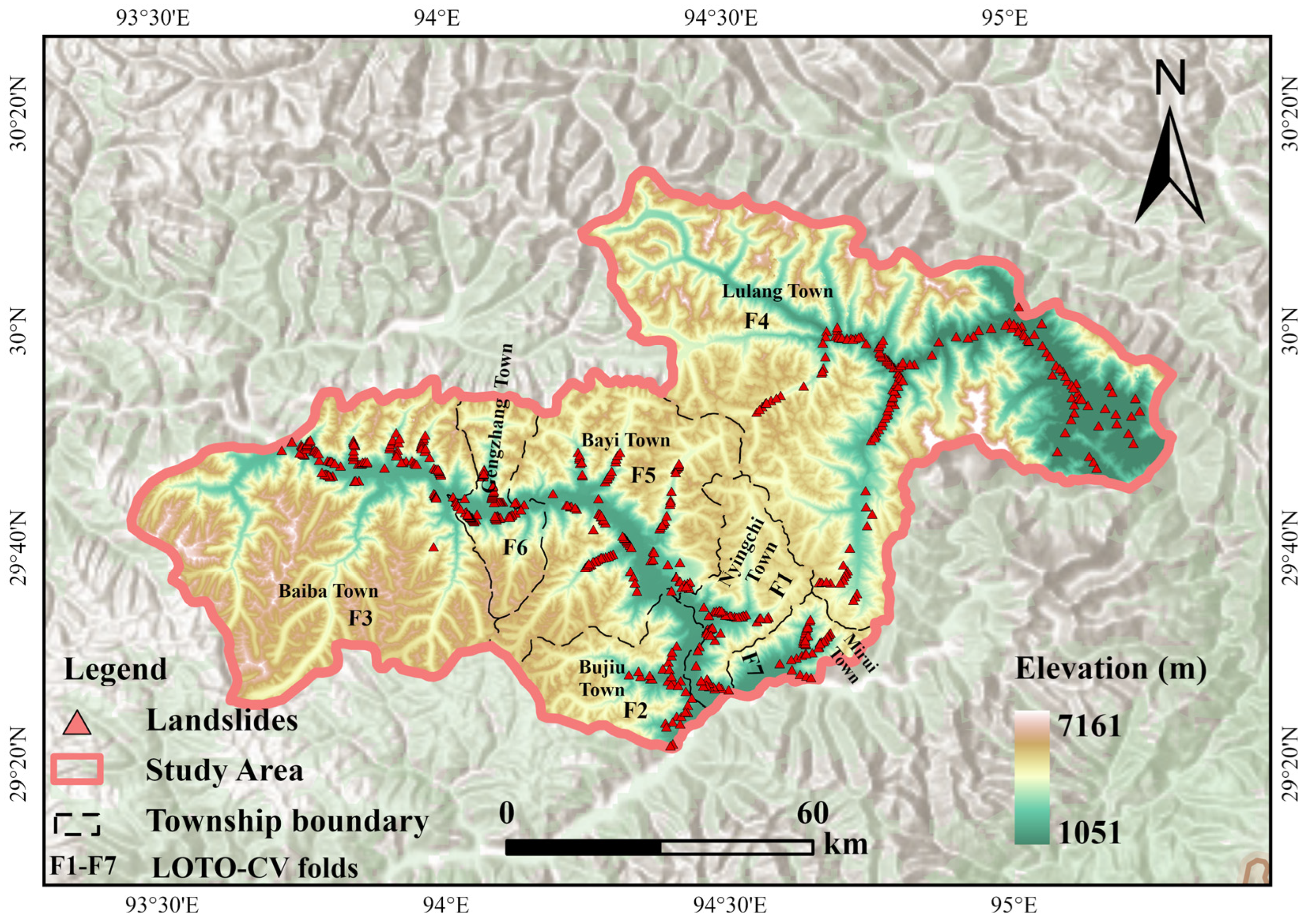
Bayi District, located in Nyingchi City, Tibet, China (29°31′–30°15′N, 93°44′–95°31′E), lies on the southeastern margin of the Qinghai–Tibet Plateau (Figure 1). The Yarlung Tsangpo River incises the Eastern Himalayan tectonic belt, forming a deeply incised canyon landscape [29,30]. The study area covers approximately 8541 km², with elevations ranging from 1051 to 7161 m.

The region is characterized by steep terrain, with a mean slope of 28.64°, and strong fluvial incision. Mean annual precipitation is approximately 1337 mm and exhibits considerable spatial variability associated with monsoonal moisture transport. Active fault systems and highly fractured bedrock are widely distributed throughout the region. Freeze–thaw processes are common in high-altitude areas, whereas ongoing road-network expansion introduces increasing anthropogenic disturbance. The combined geomorphic, climatic, geological, and anthropogenic conditions indicate that the region is prone to landslide occurrence and provides a representative setting for landslide susceptibility assessment in high-relief mountainous environments [31,32]. As the junction of the G318 national highway and the Linzhi–Lhasa expressway, Bayi District has experienced sustained road-construction activity in recent decades. Road construction and slope cutting are widespread along these corridors and may be associated with local slope instability. The spatial heterogeneity of regional conditioning factors, combined with an inventory density of approximately 0.043 landslides per km², means that model predictions in transitional terrain may be sensitive to resampling—a challenge that motivates the joint susceptibility–uncertainty assessment framework developed in this study.

2.1.2. Data and Sample Preparation

Landslide occurrence is jointly controlled by multiple geological and environmental factors. Based on previous studies and the characteristics of the high-altitude canyon environment in Bayi District, a multi-source spatial dataset was constructed [33,34]. It includes four categories: topography, hydro-meteorology, geological structure, and environmental conditions (

Table 1. Landslide conditioning factors and their data sources used in this study.

Conditioning Factors	Spatial Resolution	Temporal Coverage	Source
Elevation, Slope, Aspect, Curvature, SID, TWI, SPI	12.5 m	2010–2011	ASF a
Rainfall	1 km	2018–2023	NTPDC b
Distance to River	1:250,000	2020	NGCC c
Lithology, Distance to Fault	1:250,000	—	CGS d
NDVI	10 m	2018–2023	GEE e
Distance to Road	—	2023	OSM f
Freeze–Thaw Index	~0.1°	2018–2023	GEE e

^a ASF: Alaska Satellite Facility (https://asf.alaska.edu (accessed on 12 December 2025)); ^b NTPDC: National Tibetan Plateau/Third Pole Environment Data Center (https://data.tpdc.ac.cn (accessed on 18 December 2025)); ^c NGCC: National Geomatics Center of China (https://www.ngcc.cn (accessed on 22 December 2025)); ^d CGS: China Geological Survey (https://www.cgs.gov.cn (accessed on 26 December 2025)); ^e GEE: Google Earth Engine (https://earthengine.google.com (accessed on 5 January 2026)); ^f OSM: OpenStreetMap Contributors (https://www.openstreetmap.org (accessed on 10 January 2026)).

). A total of 14 landslide conditioning factors were selected.

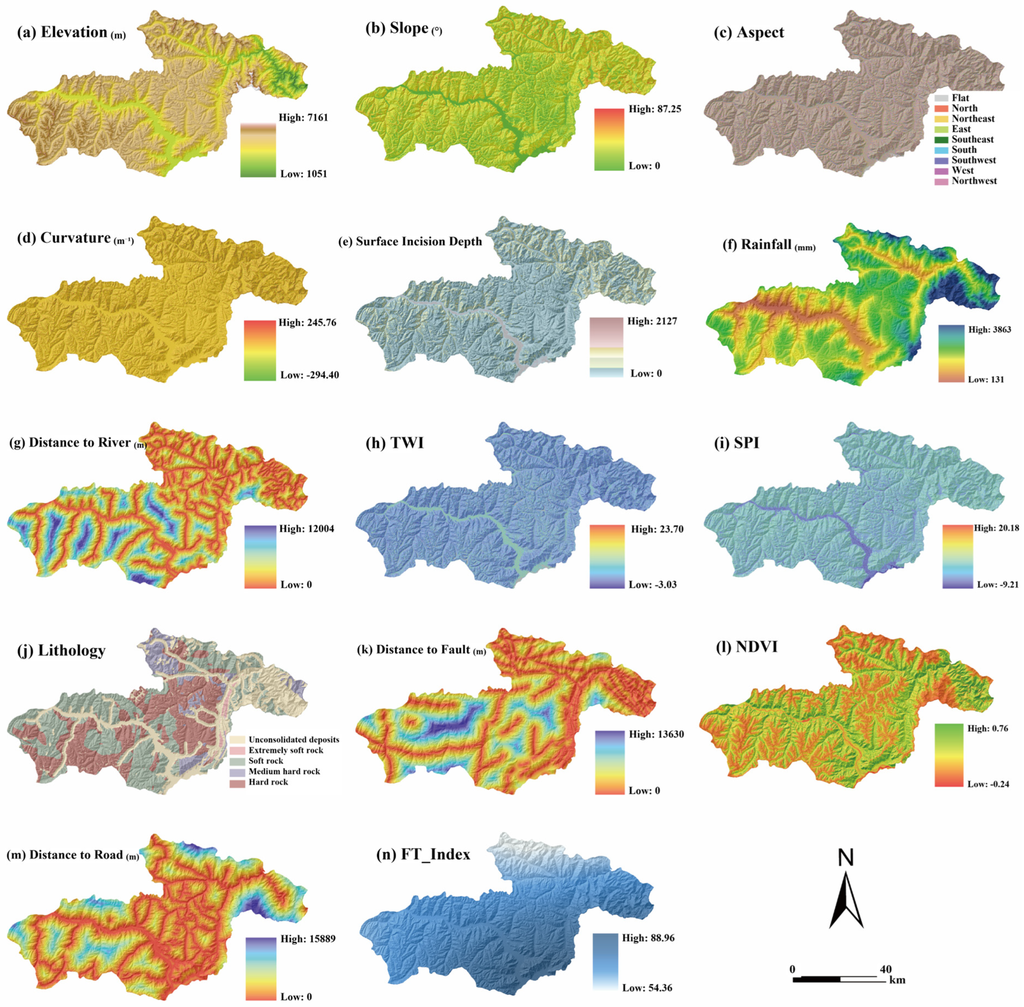
Topographic factors—elevation, slope, aspect, curvature, Surface Incision Depth (SID), TWI, and SPI—were derived from the ALOS PALSAR DEM (ASF, 12.5 m). Given the quasi-static nature of regional topography, the 2010–2011 DEM was considered suitable for deriving terrain-related predisposing factors during the landslide inventory period. Aspect was classified into Flat and eight directional categories and one-hot encoded for model fitting; the North category spans the 0°/360° boundary. Rainfall was represented by the multi-year mean annual precipitation for 2018–2023, calculated as the arithmetic mean of six annual precipitation grids. The 1-km precipitation data were obtained from the National Tibetan Plateau Data Center (NTPDC) and were generated from monthly precipitation grids interpolated from national meteorological station records. Road networks were sourced from NGCC and OSM, and lithology and fault data were digitized from a 1:250,000 regional geological map (CGS). The 2023 road dataset was used as the most complete available representation of the regional transportation network at the end of the inventory period. Lithology was reclassified into five ordered categories according to rock-mass competence: unconsolidated deposits (1), extremely soft rock (2), soft rock (3), medium-hard rock (4), and hard rock (5). The codes represent a geotechnically defined order rather than arbitrary nominal labels. The ordinal index preserves this competence gradient but does not imply equal physical spacing between classes; tree-based models can learn threshold responses, whereas LR and the RBF-SVM use it as an ordered proxy. NDVI was computed from a multi-year Sentinel-2 Level-2A median composite (COPERNICUS/S2, GEE; cloud fraction < 20%; 2018–2023) as the normalized difference between bands B8 and B4 at 10 m resolution. The freeze–thaw index was obtained from the ERA5-Land Daily Aggregated dataset (ECMWF ERA5-Land, GEE), defined as the annual count of days on which daily maximum temperature exceeded 0 °C and daily minimum temperature fell below 0 °C; a six-year average (2018–2023) was computed to reduce interannual variability. Given ERA5-Land’s native resolution of approximately 0.1° (~9 km), the derived index was resampled via bilinear interpolation to match the analysis grid. All datasets were projected to WGS 1984 UTM Zone 46N (EPSG:32646) and resampled to a uniform resolution of 12.5 m (Figure 2, Table 1). The 12.5 m grid was adopted as the analysis resolution because it matches the native pixel spacing of the ALOS PALSAR DEM—the highest-resolution primary data source—and defines the finest spatial scale at which topographic derivatives can be reliably computed in this terrain. Resampling the 1-km rainfall and approximately 9-km freeze–thaw datasets to this grid was performed for spatial alignment and did not increase their native information content.

The inventory was obtained from the 2023 Geological Hazard Census conducted by the Bayi District Transportation Bureau and contains all 370 confirmed records available for 2018–2023. All records were classified generally as landslides; detailed subtypes and event-specific dates were not consistently recorded. The CGCS2000 points represent landslide centroids, while polygon boundaries and dimensions were unavailable. The source database did not report mapping procedures, positioning instruments, or coordinate accuracy, and remote inaccessible landslides may be underrepresented. Negative samples were generated using a constrained random sampling strategy. Areas unsuitable for landslide occurrence, including permanent water bodies and low-slope plains (<5°), were excluded from the candidate area. To reduce the likelihood of including unrecorded landslides as negative samples, a 1000 m exclusion buffer was applied around all mapped landslides. This baseline distance was adopted from Fu et al. (2023), who evaluated buffers within the range of 300–1500 m and identified 1000 m as an appropriate trade-off [35]. Sensitivity was further tested for the final Stacking model at 500, 1000, and 1500 m using five independent 1:1 negative-sample realizations per distance. Negative samples were then randomly selected from the remaining area using a 1:1 positive-to-negative ratio. This strategy allows the negative samples to represent diverse environmental conditions across the study area while reducing potential spatial sampling bias [36,37].

2.2. Methods

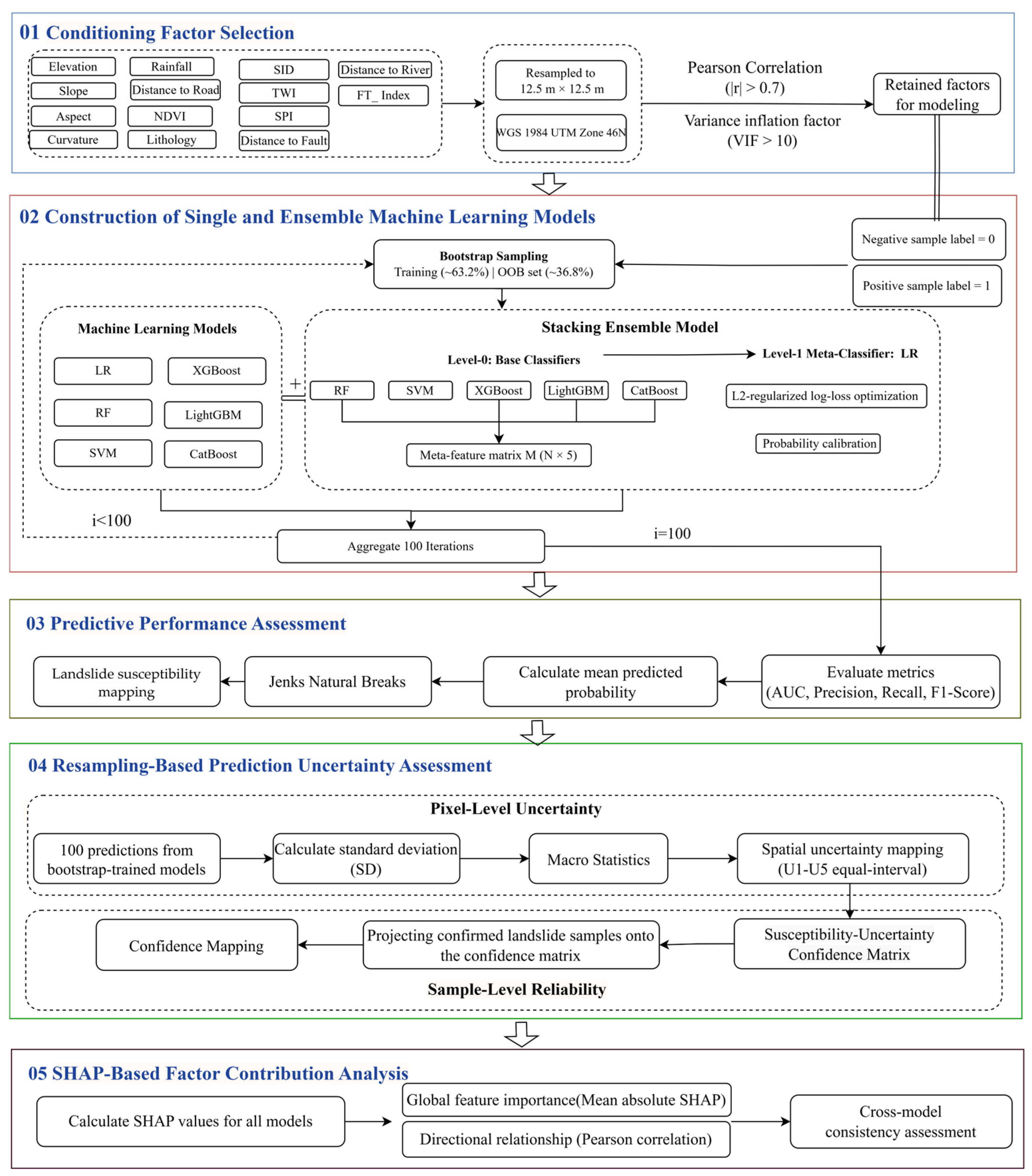
Figure 3 illustrates the proposed analytical framework. Following strict multicollinearity diagnostics to isolate robust conditioning factors, a single machine learning model and a heterogeneous Stacking ensemble model were constructed. Predictive performance was subsequently evaluated using OOB samples within 100 bootstrap iterations. The bootstrap-trained models generated in these iterations were then used for pixel-level resampling-based prediction uncertainty quantification, yielding a coupled Susceptibility–Uncertainty Confidence matrix. Finally, SHAP-based global attribution was integrated to interpret the underlying driving mechanisms. This continuous progression ensures a rigorous, end-to-end transition from initial feature refinement to transparent, reliability-aware susceptibility assessment.

2.2.1. Conditioning Factor Selection

Collinearity among the 14 candidate conditioning factors was assessed through a sequential two-step procedure. Pairwise Pearson correlation coefficients were computed to identify strongly correlated factor pairs, with |r| > 0.7 adopted as the redundancy threshold [38,39]. Variance inflation factor (VIF) analysis was subsequently applied to detect multicollinearity involving three or more variables, with VIF > 10 as the removal criterion [40,41]. Factors exceeding these thresholds were iteratively removed in order of severity, and both diagnostics were recalculated after each removal step until all remaining factors satisfied the criteria. The retained factors were carried forward for all subsequent modeling.

2.2.2. Construction of Single and Ensemble Machine Learning Models

• Single Machine Learning Models

Six classifiers were constructed as standalone models for comparative evaluation: Logistic Regression (LR), Support Vector Machine (SVM), Random Forest (RF), XGBoost, LightGBM, and CatBoost. These models represent three algorithmic paradigms: linear methods, kernel-based methods, and tree-based ensemble methods [42,43]. This design facilitates a structured comparison of modeling behavior across different levels of nonlinearity and feature interaction. Among them, LR also serves as the Level-1 meta-classifier within the Stacking framework; evaluating it here as a standalone model isolates its independent predictive capacity relative to the ensemble approach.

For the three gradient boosting models (XGBoost, LightGBM, and CatBoost), the number of estimators was set to 300, the learning rate to 0.05, and the maximum tree depth to 6. For RF, the number of estimators was set to 300 and the maximum tree depth to 10; no learning rate parameter applies under the bagging framework. LR was trained with a maximum of 1000 iterations, and SVM used the RBF kernel. All remaining parameters were left at their default settings [44]. All hyperparameters were specified before model evaluation and were not selected using the OOB or LOTO-CV results. The settings were chosen as conservative model configurations, with moderate tree depths, shrinkage-based learning rates, and standard regularization parameters used to limit model complexity. The reported results therefore compare prespecified model configurations rather than the optimally tuned performance of each algorithm. Parameter rationales are provided in Appendix A,

Table A1. Hyperparameter ranges examined in the robustness analysis.

Model	Reported Configuration	Examined Values	Rationale
LR	C = 1	C: 0.1, 1, 10	Standard L2 regularization
SVM	C = 1; gamma = scale	C: 0.1, 1, 10; gamma: scale, 0.01, 0.1	Standard penalty and variance-scaled kernel
RF	n = 300; depth = 10	n: 200, 300, 500; depth: 8, 10, None	Stable ensemble with constrained depth
XGBoost	n = 300; rate = 0.05; depth = 6	n: 200, 300, 500; rate: 0.03, 0.05, 0.10; depth: 4, 6, 8	Conservative shrinkage and moderate depth
LightGBM	n = 300; rate = 0.05; depth = 6	n: 200, 300, 500; rate: 0.03, 0.05, 0.10; depth: 4, 6, 8	Conservative shrinkage and controlled depth
CatBoost	n = 300; rate = 0.05; depth = 6	n: 200, 300, 500; rate: 0.03, 0.05, 0.10; depth: 4, 6, 8	Conservative shrinkage and moderate depth
Stacking	Meta-learner C = 1	C: 0.1, 1, 10	Regularized LR meta-learner

[45,46].

Continuous predictors were standardized using Z-score transformation for LR and SVM. In each resampling or cross-validation fold, the means and standard deviations were estimated exclusively from the training data and subsequently applied to the corresponding validation or test data.

2.

Stacking Ensemble Model

A two-layer heterogeneous Stacking model was constructed to leverage the complementary predictive characteristics of the baseline classifiers. Five models—SVM, RF, XGBoost, LightGBM, and CatBoost—formed the Level-0 base learner set; LR was reserved as the Level-1 meta-classifier.

To prevent data leakage during meta-feature construction, a 5-fold out-of-fold (OOF) strategy was applied at Level-0. Each base model was trained on four folds and used to predict the held-out fold; predictions across all folds were concatenated to form a $N\times 5$ meta-feature matrix:

$$Z_i=\left({\widehat{p}}_{i1},{\widehat{p}}_{i2},{\widehat{p}}_{i3},{\widehat{p}}_{i4},{\widehat{p}}_{i5}\right)$$

(1)

where $Z_i$ denotes the meta-feature vector for the $i$-th sample, and ${\widehat{p}}_{ik}$ represents the OOF prediction probability generated by the $k$-th base learner.

This procedure helps ensure that Level-1 meta-learning is performed on out-of-fold predictions that were not observed during Level-0 training, thereby reducing the risk of secondary overfitting [37,47,48].

LR was selected as the meta-classifier because the meta-feature matrix already encodes a nonlinear probabilistic representation extracted by structurally diverse base learners; a linear combiner provides a relatively simple ensemble weighting strategy without introducing substantial additional model complexity. The final Stacking prediction is expressed as:

$$P_i=\sigma \left({\beta }_0+{\displaystyle \sum _{k=1}^5{\beta }_k}{p}_{ik}\right)$$

(2)

where $P_i$ denotes the final predicted landslide probability for sample $i$, ${\beta }_0$ is the intercept term, ${\beta }_k$ is the ensemble weight assigned to the $k$-th base learner, and $\sigma (·)$ is the sigmoid activation function.

3.

Probability Calibration

Final probability outputs from all seven models were calibrated using sigmoid calibration. Within each resampling or validation fold, the calibrator was fitted using five-fold out-of-fold predictions from the training data only; calibration was applied to the final output of the Stacking model.

2.2.3. Predictive Performance Assessment

Predictive performance was assessed through two complementary approaches: bootstrap-based OOB resampling and LOTO-CV. Landslide density across susceptibility classes was additionally calculated to describe the class-level distribution of mapped landslides within each model.

Model performance was evaluated using a unified 100-iteration bootstrap out-of-bag OOB resampling framework. In each iteration, a stratified training set was sampled with replacement from the full dataset, with unselected samples forming the OOB test set; AUC, precision, recall, and F1-score were averaged across iterations, with AUC adopted as the primary metric for its threshold independence and robustness to class imbalance [49,50,51]. Precision, recall, and F1-score were calculated using a probability threshold of 0.50. OOB results are reported as mean ± SD across 100 bootstrap iterations, whereas LOTO-CV results are reported as mean ± SD across the seven township folds. Paired bootstrap 95% confidence intervals compared Stacking with CatBoost under OOB; LOTO-CV comparisons are descriptive. Because landslides cluster spatially in mountainous terrain, random OOB partitioning can place training and test samples in close proximity, inflating apparent performance through spatial autocorrelation. LOTO-CV was conducted using the seven townships of Bayi District as spatial partitioning units: in each fold, one township was withheld for testing while the remaining six formed the training set, with a nested out-of-fold procedure re-executed for the Stacking model to avoid leakage during meta-feature construction. To further reduce potential spatial dependence across adjacent township boundaries, a 1-km buffered LOTO-CV sensitivity analysis was conducted for the final Stacking model. In each fold, all samples within the withheld township were retained as the test set, while training samples located within 1 km outside its boundary were excluded. As an additional within-model spatial consistency check, landslide density was calculated for each susceptibility class, defined as confirmed landslide points per 100 km² of class area, to assess whether higher predicted classes contained greater landslide concentrations. To evaluate whether model performance depended on distance to roads, the complete Stacking ensemble was retrained after excluding this factor, while retaining the same samples, model settings, and OOB and leave-one-township-out cross-validation procedures.

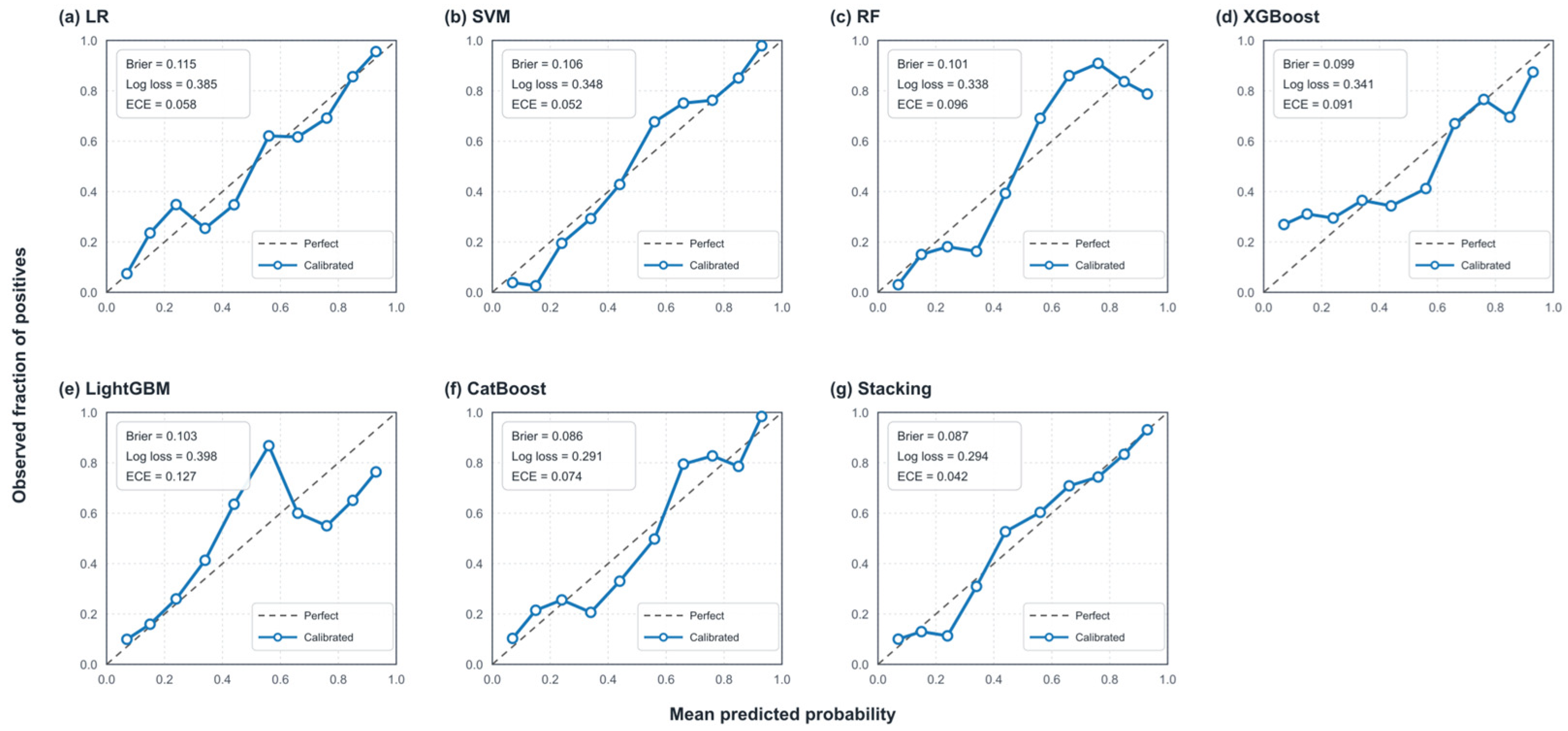
Calibration was evaluated from pooled LOTO-CV test predictions using reliability diagrams with ten equal-frequency bins, Brier score, log loss, and sample-weighted ECE. Formal cross-model comparisons were based on unclassified predicted probabilities evaluated using identical samples and validation partitions. AUC assessed discrimination, Brier score and log loss assessed probabilistic accuracy, and ECE and calibration curves were used as supplementary calibration diagnostics.

For spatial prediction, the mean predicted probability generated by the 100 bootstrap-trained models was taken as the final susceptibility estimate for each pixel, producing continuous probability surfaces at 12.5 m resolution. Predictions were processed in overlapping sub-blocks before mosaicking into a full-domain raster, a strategy applied uniformly across all models [52].

2.2.4. Resampling-Based Prediction Uncertainty Assessment

Resampling-based prediction variability was evaluated across both pixel and sample dimensions. At the pixel-level, the standard deviation of 100 predictions generated by the bootstrap-trained models, coupled with spatial prediction-SD mapping, was used to characterize uncertainty, providing spatially explicit measures of prediction variability arising from limited training data and model assumptions. At the sample-level, the reliability of predictions was assessed by projecting the 370 confirmed landslide samples onto the susceptibility–uncertainty confidence matrix, enabling comparison of how high-susceptibility predictions align with regions of high model confidence. Together, these two perspectives allow a comprehensive evaluation of both the local variability and the reliability of model outputs.

• Pixel-Level Prediction SD Quantification

The 100 bootstrap iterations established in Section 2.2.3 generate, for each spatial pixel, an empirical sequence of 100 predictions produced by the bootstrap-trained models:

$${𝒫}_i=\left\{P_{i,1},P_{i,2},\dots ,P_{i,B}\right\}$$

(3)

where $P_{i,b}$ denotes the predicted probability for pixel $i$ during the $b$-th bootstrap iteration, and $B=100$.

The pixel-wise mean prediction was adopted as the susceptibility estimate:

$${\mu }_i={\displaystyle \frac{1}{B}}{\displaystyle \sum _{b=1}^B{P}_{i,b}}$$

(4)

The standard deviation of the prediction sequence was adopted as a pixel-level measure of resampling-based predictive variability arising from changes in training-sample composition. It does not represent a complete estimate of epistemic uncertainty because inventory errors, input-data uncertainty, hyperparameter uncertainty, and alternative model structures were not propagated through the analysis [20,21]:

$${\sigma }_i=\sqrt{{\displaystyle \frac{1}{B-1}}{\displaystyle \sum _{b=1}^B{(P_{i,b}-{\mu }_i)}^2}}$$

(5)

A higher ${\sigma }_i$ indicates that model behavior is sensitive to training set composition, reflecting lower spatial reliability; a lower ${\sigma }_i$ reflects convergent predictions across resampling iterations, indicating higher confidence in the susceptibility estimate. The number of iterations (B = 100) is consistent with empirical evidence that prediction statistics stabilize within 80–120 iterations at comparable sample sizes [53].

In an additional 100-iteration analysis for the final Stacking model, the negative dataset was regenerated before each bootstrap iteration to incorporate negative-sample selection variability into the pixel-wise SD.

2.

Sample-Level Reliability Assessment

To move beyond the parallel presentation of separate susceptibility and uncertainty maps—a limitation common to existing LSM uncertainty studies—the two outputs were integrated into a unified spatial representation. The five susceptibility levels (L1–L5, Section 2.2.3) and five uncertainty levels (U1–U5) were cross-tabulated to construct a confidence matrix in which each cell represents a distinct combination of predicted susceptibility level and prediction reliability [53]. This joint representation addresses the interpretive gap between high susceptibility and high-confidence susceptibility, a distinction that single-output probability maps cannot convey.

Uncertainty levels U1–U5 were defined by equal-interval SD thresholds of 0.05, 0.10, 0.15, and 0.20 over the operational range [0, 0.20]. Prior to discretization, SD values were truncated at the 95th percentile to limit the influence of extreme outliers on classification boundaries. The equal-interval scheme was adopted to maintain consistent classification granularity across models and to facilitate comparison under differing uncertainty magnitude distributions. The upper bound of 0.20 was selected to encompass the dominant range of spatial variation in prediction stability while excluding the sparse high-uncertainty tail concentrated in poorly constrained boundary regions.

The 370 confirmed landslide samples were projected onto the confidence matrix to assess whether high-susceptibility predictions spatially coincide with low-uncertainty predictions. The matrix was subsequently reclassified into four spatial decision quadrants by applying dual thresholds along both the susceptibility and uncertainty dimensions, distinguishing areas by both susceptibility level and prediction confidence. This quadrant structure provides the spatial basis for the reliability-aware interpretation presented in Section 3.3 and Section 4.2. Sensitivity of the Stacking confidence matrix was evaluated using alternative SD truncation levels, ±20% uncertainty thresholds, and alternative classification schemes, with robustness measured by spatial agreement, Cohen’s kappa, L5–U1 Jaccard index, and landslide allocation.

2.2.5. SHAP-Based Factor Contribution Analysis

SHAP (SHapley Additive Explanations) was applied post hoc to quantify conditioning-factor contributions [54,55]. SHAP values were calculated separately for all seven models using their held-out LOTO-CV samples. For Stacking, KernelExplainer was applied to the final output of the complete pipeline, with the fold-specific training data used as the background dataset. Values were pooled across folds; the eight aspect dummy-variable SHAP values were summed for each sample, and global importance was calculated as the mean absolute attribution of the 12 original factors.

The SHAP value for feature $i$ is defined as:

$${\varphi }_i={\displaystyle \sum _{S\subseteq N\setminus \left\{i\right\}}\frac{\left|S\right|!(|N|-|S|-1)!}{\left|N\right|!}}\left[v(S\cup \{i\})-v(S)\right]$$

(6)

where $N$ denotes the complete feature set, $S$ represents a subset excluding feature $i$, and $v\left(S\right)$ is the expected model output conditioned on subset $S$.

To characterize the directional relationship between each conditioning factor and predicted landslide probability, the Pearson correlation coefficient between raw feature values and their corresponding SHAP values was calculated. The sign of this coefficient indicates the direction of association between a conditioning factor and predicted landslide susceptibility, while its magnitude reflects the strength of that relationship.

SHAP analysis was conducted separately for all seven models. Cross-model consistency in feature importance rankings was assessed to evaluate whether dominant factors were stably identified regardless of the underlying algorithm. This consistency check provides additional interpretive support for the robustness of the modeled factor–response relationships, independent of any single model’s behavior.

3. Results

3.1. Conditioning Factor Characteristics

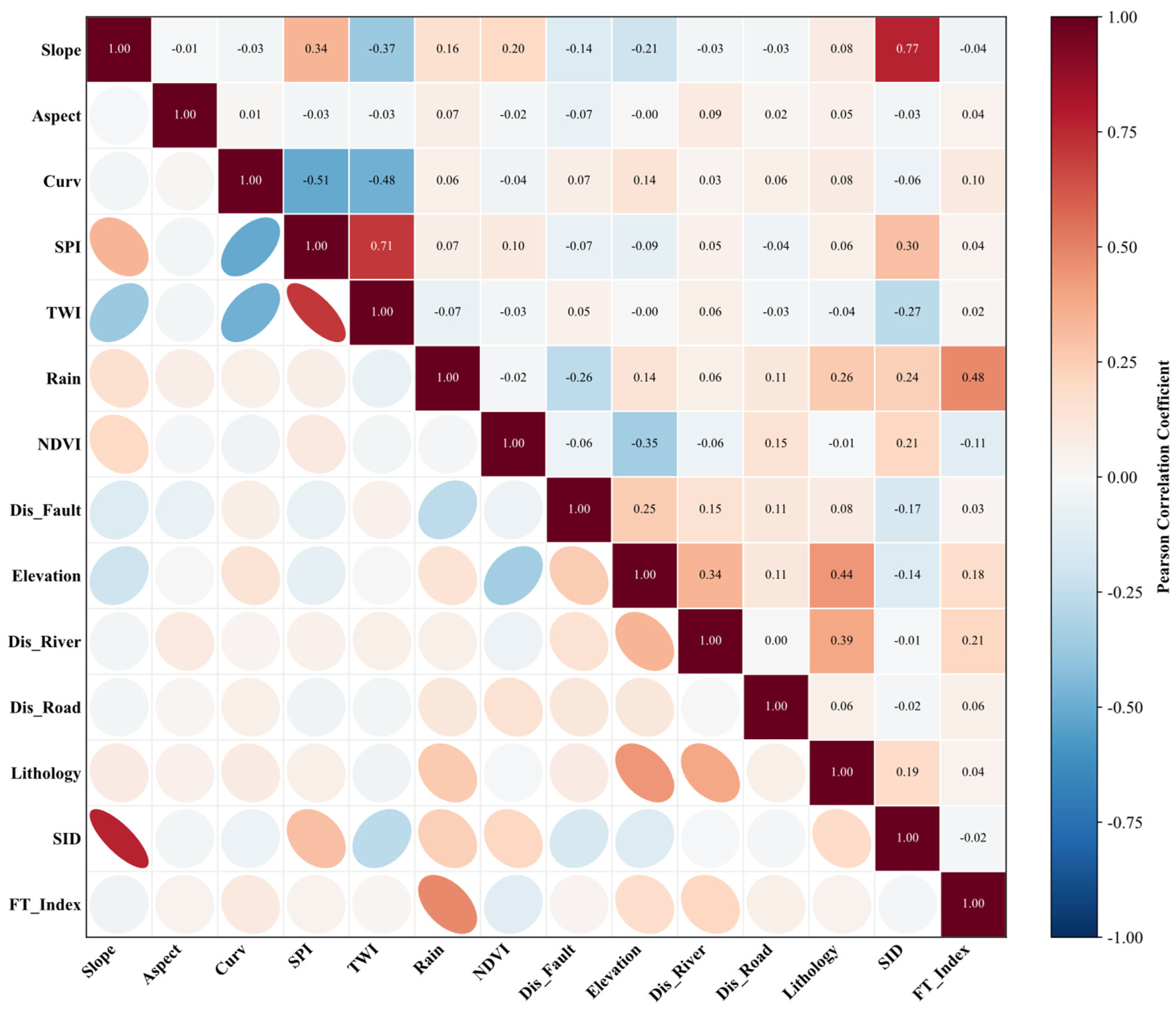
To resolve the identified collinearity, a stepwise removal procedure was applied. The Pearson correlation matrix (Figure 4) indicated strong pairwise correlations between TWI and SPI (r = 0.71) and between SID and slope (r = 0.77). Among the collinear pairs, TWI exhibited the highest VIF value (15.07) across all 14 factors (

Table 2. VIF values before and after removing TWI and SID.

Conditioning Factor	Initial VIF	Final VIF	Conditioning Factor	Initial VIF	Final VIF
Slope	9.04	3.41	Distance to Fault	1.26	1.21
Aspect	1.03	1.02	Elevation	1.77	1.77
Curvature	1.46	1.39	Distance to River	1.35	1.35
SPI	9.76	2.63	Distance to Road	1.09	1.09
TWI	15.07	Removed	Lithology	1.61	1.61
Rainfall	1.73	1.61	SID	2.76	Removed
NDVI	1.31	1.27	Freeze–Thaw Index	1.55	1.44

) and was therefore removed first. SPI was retained because it captures overland flow accumulation dynamics that are physically distinct from the slope-weighted wetness index represented by TWI, and its removal was not warranted once TWI was excluded. SID was subsequently excluded rather than slope for two reasons. Slope is a direct proxy for gravitational shear stress and constitutes the primary mechanical driver of shallow landslide initiation; the terrain dissection information encoded in SID is largely recoverable from the slope–elevation combination already retained. Additionally, while SID carried a lower VIF (2.76) than slope (9.04), slope remained sub-threshold and its superior geomechanical relevance took precedence in the removal decision (Figure 4, Table 2). Following the removal of TWI and SID, VIF values were recalculated for the final 12 predictors and ranged from 1.02 to 3.41, with all values below the threshold of 10. Aspect was represented by eight dummy variables with North omitted as the reference category, and the single Aspect value reported in Table 2 represents the maximum VIF among these dummy variables.

3.2. Predictive Accuracy Comparison

Following feature selection, model performance was evaluated through 100 bootstrap-based OOB resampling and LOTO-CV, with results for both frameworks summarized in

Table 3. Comparison of predictive performance under (a) OOB and (b) LOTO-CV frameworks.

(a) OOB results
Model	AUC	Precision	Recall	F1
LR	0.8885 ± 0.0196	0.8215 ± 0.0281	0.8140 ± 0.0304	0.8177 ± 0.0248
SVM	0.9090 ± 0.0173	0.8285 ± 0.0257	0.8345 ± 0.0279	0.8315 ± 0.0226
RF	0.9280 ± 0.0149	0.8510 ± 0.0218	0.8615 ± 0.0231	0.8561 ± 0.0192
XGBoost	0.9220 ± 0.0167	0.8470 ± 0.0235	0.8505 ± 0.0256	0.8487 ± 0.0214
LightGBM	0.9315 ± 0.0154	0.8550 ± 0.0229	0.8675 ± 0.0217	0.8612 ± 0.0198
CatBoost	0.9405 ± 0.0136	0.8585 ± 0.0202	0.8835 ± 0.0194	0.8708 ± 0.0171
Stacking	0.9780 ± 0.0089	0.9250 ± 0.0156	0.9380 ± 0.0148	0.9315 ± 0.0127
(b) LOTO-CV results
Model	AUC	Precision	Recall	F1
LR	0.8410 ± 0.0280	0.8090 ± 0.0340	0.7200 ± 0.0410	0.7619 ± 0.0350
SVM	0.8600 ± 0.0240	0.8260 ± 0.0300	0.7430 ± 0.0360	0.7823 ± 0.0310
RF	0.8830 ± 0.0210	0.8490 ± 0.0270	0.7570 ± 0.0330	0.8004 ± 0.0280
XGBoost	0.8760 ± 0.0230	0.8370 ± 0.0290	0.7480 ± 0.0350	0.7900 ± 0.0300
LightGBM	0.8860 ± 0.0190	0.8440 ± 0.0250	0.7580 ± 0.0310	0.7987 ± 0.0260
CatBoost	0.8900 ± 0.0200	0.8530 ± 0.0240	0.7640 ± 0.0280	0.8061 ± 0.0250
Stacking	0.9216 ± 0.0165	0.8589 ± 0.0156	0.7971 ± 0.0178	0.8269 ± 0.0168

Note: Values are presented as mean ± SD. OOB statistics were calculated across 100 bootstrap iterations, whereas LOTO-CV statistics were calculated across the seven township folds.

.

Under OOB resampling, LR and SVM showed comparatively lower predictive capability, with AUC values of 0.8885 and 0.9090, respectively. The tree-based ensemble models (RF, XGBoost, LightGBM, and CatBoost) performed better, reflecting stronger nonlinear fitting in this complex mountainous setting, with CatBoost reaching the best single-model AUC (0.9405). The Stacking model outperformed all single models under OOB, achieving the highest AUC (0.9780) and F1-score (0.9315). Stacking outperformed CatBoost by 0.0375 in OOB AUC (95% CI: 0.0174–0.0572) and by 0.0607 in OOB F1-score (95% CI: 0.0318–0.0889). Because both confidence intervals excluded zero, the performance improvements were statistically supported.

Under LOTO-CV, every model showed a performance drop relative to its OOB estimate, indicating reduced predictive performance when the models were transferred to a geographically withheld township. Stacking showed the highest observed mean LOTO-CV AUC (0.9216) among the seven models, with a reduction of 0.056 from its OOB value, comparable to the average reduction across single models (0.047). The observed mean-AUC ranking matched the OOB ranking; no paired statistical comparison was conducted for LOTO-CV. Fold-level results for the Stacking model (

Table 4. Fold-level LOTO-CV results of the Stacking model across seven townships.

Fold	Township	Positive Samples	Negative Samples	AUC	Precision	Recall	F1
1	Linzhi	59	30	0.935	0.873	0.814	0.842
2	Bujiu	51	25	0.947	0.882	0.823	0.852
3	Baiba	42	50	0.931	0.865	0.807	0.835
4	Lulang	73	115	0.901	0.838	0.776	0.806
5	Bayi	62	90	0.917	0.856	0.791	0.822
6	Gengzhang Menba	34	35	0.909	0.844	0.780	0.811
7	Mirui	49	25	0.911	0.854	0.789	0.820
—	Mean ± SD	—	—	0.9216 ± 0.0165	0.8589 ± 0.0156	0.7971 ± 0.0178	0.8269 ± 0.0168

Note: The final row reports the unweighted mean ± sample SD across the seven township folds.

) ranged from AUC 0.901 to 0.947 across the seven townships, with the lowest value recorded for Lulang Township—the fold with the largest sample size and the greatest terrain complexity, reflecting the difficulty of generalizing across that subregion’s heterogeneous incised-valley terrain. The consistency of performance across folds indicates acceptable spatial generalizability of the Stacking model within Bayi District. Across the locally examined settings, the maximum improvements over the reported configurations were 0.0126 in LOTO-CV AUC and 0.0104 in F1-score, while the reported settings were retained without using these results for parameter selection. Minor ranking changes occurred among RF, XGBoost, and LightGBM; however, CatBoost had the highest observed AUC among the single-model configurations when the upper values within the tested ranges were compared, and Stacking had the highest observed mean AUC (Appendix A,

Table A2. LOTO-CV performance ranges obtained in the hyperparameter robustness analysis.

Model	Reported AUC	Tested AUC Range	Reported F1	Tested F1 Range
LR	0.8410	0.8324–0.8432	0.7619	0.7495–0.7650
SVM	0.8600	0.8421–0.8709	0.7823	0.7584–0.7896
RF	0.8830	0.8792–0.8870	0.8004	0.7938–0.8041
XGBoost	0.8760	0.8615–0.8886	0.7900	0.7721–0.8004
LightGBM	0.8860	0.8728–0.8890	0.7987	0.7810–0.8022
CatBoost	0.8900	0.8796–0.8952	0.8061	0.7935–0.8100
Stacking	0.9216	0.9178–0.9235	0.8269	0.8210–0.8284

).

After excluding distance to roads, the Stacking model achieved an OOB AUC of 0.9630 and an OOB F1-score of 0.9216, compared with 0.9780 and 0.9315, respectively, for the original model. Its LOTO-CV AUC decreased from 0.9216 to 0.918, while its LOTO-CV F1-score decreased from 0.8269 to 0.8153. These limited changes indicate that the model retained stable predictive performance after removing distance to roads.

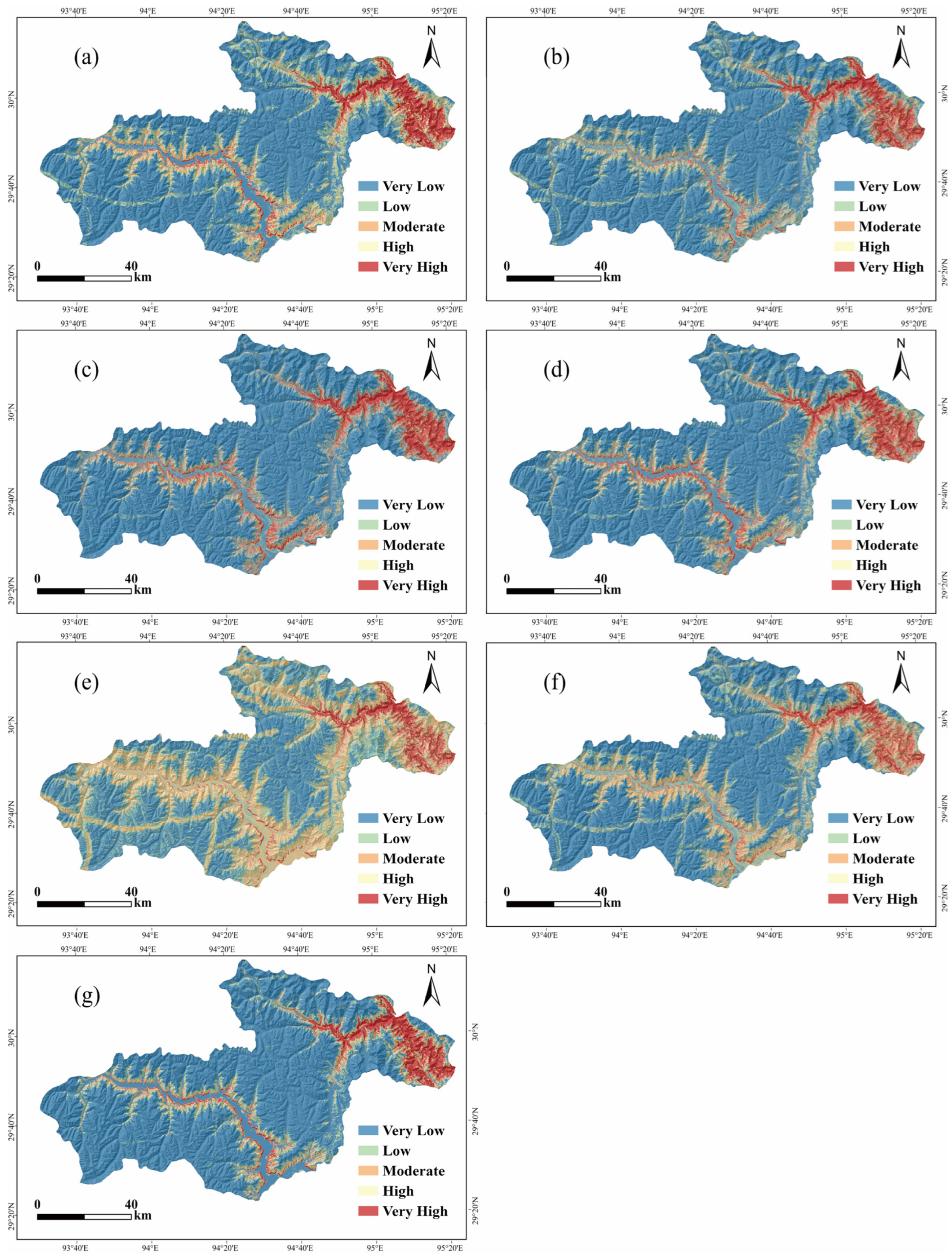
The 1-km buffered LOTO-CV sensitivity analysis yielded an AUC of 0.914 and an F1-score of 0.8142 for the Stacking model, compared with 0.922 and 0.8269, respectively, under the original LOTO-CV (Appendix A,

Table A3. Fold-level sample changes and predictive performance under 1-km buffered LOTO-CV.

Fold	Township	Original Training Samples	Samples Excluded by Buffer	Buffered Training Samples	Test Samples	Buffered AUC	Buffered F1
1	Linzhi	651	24	627	89	0.928	0.832
2	Bujiu	664	18	646	76	0.940	0.843
3	Baiba	648	31	617	92	0.923	0.826
4	Lulang	552	36	516	188	0.893	0.792
5	Bayi	588	29	559	152	0.910	0.813
6	Gengzhang Menba	671	17	654	69	0.904	0.798
7	Mirui	666	15	651	74	0.900	0.795

). The decreases of 0.008 in AUC and 0.0127 in F1-score indicate that model performance remained stable after increasing the spatial separation between the training and test samples. Across the tested buffer distances and negative-sample realizations, mean LOTO-CV AUC ranged from 0.9110 to 0.9239 and mean F1-score from 0.8125 to 0.8294, indicating limited sensitivity to negative-sample selection (Appendix A,

Table A4. Sensitivity of Stacking performance to buffer distance and negative-sample realization.

Buffer Distance	Realizations	OOB AUC	OOB F1	LOTO-CV AUC	LOTO-CV F1
500 m	5	0.9678 ± 0.0019	0.9189 ± 0.0018	0.9110 ± 0.0026	0.8125 ± 0.0031
1000 m	5	0.9754 ± 0.0019	0.9286 ± 0.0020	0.9205 ± 0.0020	0.8244 ± 0.0033
1500 m	5	0.9794 ± 0.0014	0.9331 ± 0.0015	0.9239 ± 0.0017	0.8294 ± 0.0022

). Calibration curves and metrics are presented in Figure 5. Brier scores ranged from 0.086 to 0.115 and log-loss values from 0.291 to 0.398; Stacking had the lowest ECE (0.042), while CatBoost had the lowest Brier score and log loss. The spatial distributions of landslide susceptibility generated by different models are shown in Figure 6.

Landslide density was calculated within the model-specific Jenks classes as a descriptive within-model analysis (

Table 5. Landslide density statistics across susceptibility classes for all models.

Model	Class	Area (km2)	Landslides (n)	Density (Landslides/100 km2)
LR	Very Low	5370.50	6	0.11
	Low	904.20	22	2.43
	Moderate	836.80	87	10.40
	High	405.30	107	26.40
	Very High	1024.39	148	14.45
SVM	Very Low	3322.50	9	0.27
	Low	2650.40	23	0.87
	Moderate	1510.80	63	4.17
	High	643.60	103	16.01
	Very High	413.89	172	41.55
RF	Very Low	5588.30	0	0.00
	Low	1386.50	6	0.43
	Moderate	556.90	25	4.49
	High	308.20	117	37.96
	Very High	701.29	222	31.66
XGBoost	Very Low	6118.20	2	0.03
	Low	1132.80	8	0.71
	Moderate	443.50	43	9.70
	High	236.40	106	44.84
	Very High	610.29	211	34.57
LightGBM	Very Low	6083.50	1	0.02
	Low	802.60	5	0.62
	Moderate	431.20	28	6.49
	High	292.80	108	36.89
	Very High	931.09	228	24.49
CatBoost	Very Low	6052.80	0	0.00
	Low	946.50	2	0.21
	Moderate	468.30	14	2.99
	High	307.10	110	35.82
	Very High	766.49	244	31.83
Stacking	Very Low	6455.50	1	0.02
	Low	866.20	1	0.12
	Moderate	345.80	2	0.58
	High	223.50	67	29.98
	Very High	650.19	299	45.98

). Because the same inventory was used for model construction, this analysis was not treated as independent validation. For all models, density generally increased toward the higher susceptibility classes, although the pattern was not strictly monotonic in every case. These local reversals may arise from small class-specific sample counts and the locations of the model-specific Jenks breaks. Within the Stacking classification, the Very High class contained 299 of the 370 confirmed landslides and had a density of 45.98 per 100 km², compared with 0.02 per 100 km² in the Very Low class. Because Jenks boundaries were calculated separately, these class-level statistics were not used for direct model ranking.

3.3. Resampling-Based Prediction Uncertainty Analysis

Conventional landslide susceptibility maps depict the spatial variation in modeled susceptibility, but susceptibility values alone cannot fully reflect prediction reliability. To further examine whether improved predictive performance was accompanied by more stable prediction behavior, resampling-based predictive variability was evaluated using the standard deviation (SD) of predictions generated by 100 bootstrap-trained models. The SD reflects prediction variability under repeated resampling and was used here as a proxy for model sensitivity to training-data perturbation. Prediction SD characteristics were analyzed from both statistical distributions and spatial patterns.

3.3.1. Statistical Distribution Characteristics of Prediction Variability

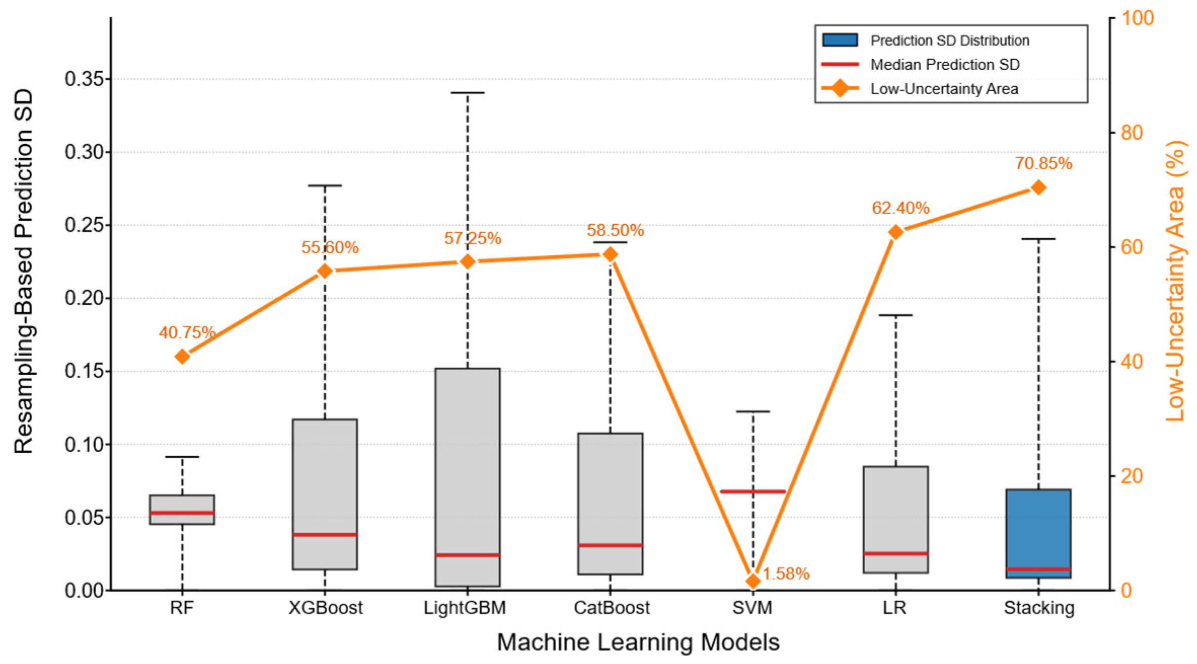
The statistical distributions of prediction SD after 95% percentile truncation are shown in Figure 7. Clear differences in prediction SD characteristics were observed among models, indicating that predictive accuracy and prediction stability were not necessarily equivalent.

Although LightGBM and CatBoost achieved relatively high predictive performance (AUC > 0.93), their prediction SD distributions exhibited noticeable dispersion. LightGBM, for instance, had a median SD of 0.024, with only 57.25% of the study area classified as low-uncertainty (SD < 0.05), indicating that high predictive performance does not necessarily imply low sensitivity to sample perturbation in spatial predictions.

The RF model showed a relatively concentrated prediction SD distribution with moderate overall stability. The LR model, despite its lower predictive accuracy, produced comparatively low prediction SD—suggesting that smoother, less flexible models may yield spatially stable predictions while lacking sufficient nonlinear discrimination. Lower prediction SD was therefore not consistently associated with higher predictive performance.

The SVM model exhibited a narrow SD distribution but an extremely limited proportion of low-uncertainty areas (1.58%), reflecting constrained spatial variability in probability outputs under repeated resampling. This behavior differed substantially from the other models, indicating that prediction SD characteristics can vary considerably across algorithmic structures.

Under OOB, Stacking had the highest mean AUC and F1-score and the lowest resampling-based prediction uncertainty. The median SD was 0.015, and 70.85% of the study area was classified as low-uncertainty. Relative to individual models, the Stacking framework showed substantially reduced prediction dispersion and more stable spatial responses under repeated resampling, suggesting that the ensemble structure contributes to both improved discrimination and greater prediction stability.

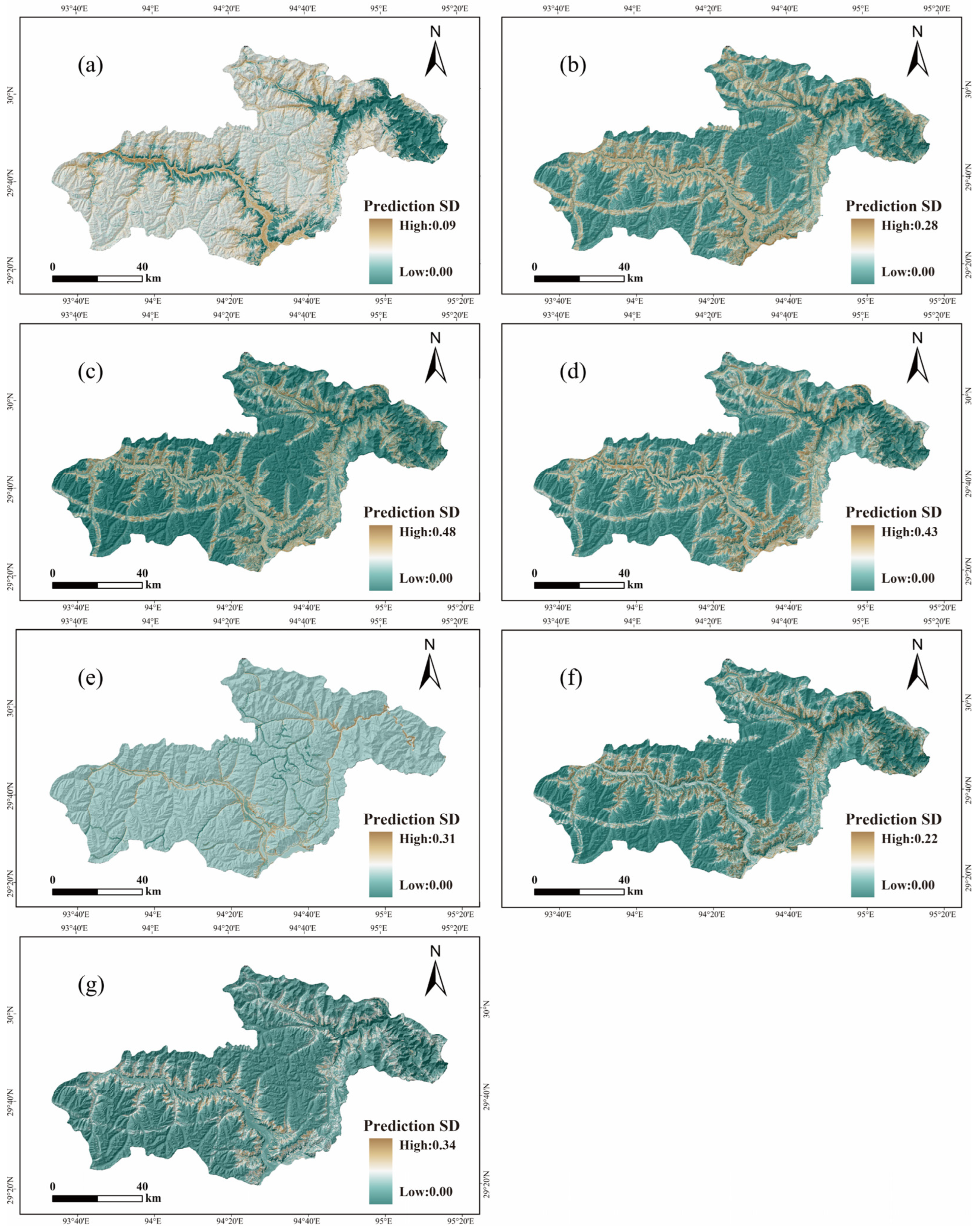
The spatial distributions of prediction SD further reflected these differences (Figure 8). In the Stacking model, high-uncertainty regions were concentrated near lithological transition zones and deeply incised valley margins, while low-uncertainty regions formed relatively continuous spatial patterns. Several single models, by contrast, exhibited more fragmented prediction SD distributions, indicating greater local sensitivity to training-data perturbation. Incorporating negative-sample selection increased the median SD from 0.0150 to 0.0183 and reduced the low-uncertainty area from 70.85% to 68.42%, while the uncertainty classes retained 91.7% spatial agreement (Appendix A,

Table A5. Effect of negative-sample selection on Stacking prediction uncertainty.

Uncertainty Scheme	Iterations	Median SD	Low-Uncertainty Area (%)	Spatial Agreement (%)
Fixed negative dataset	100	0.0150	70.85	100.0
Negative dataset regenerated in each iteration	100	0.0183	68.42	91.7

).

3.3.2. Confidence Matrix Sample Mapping

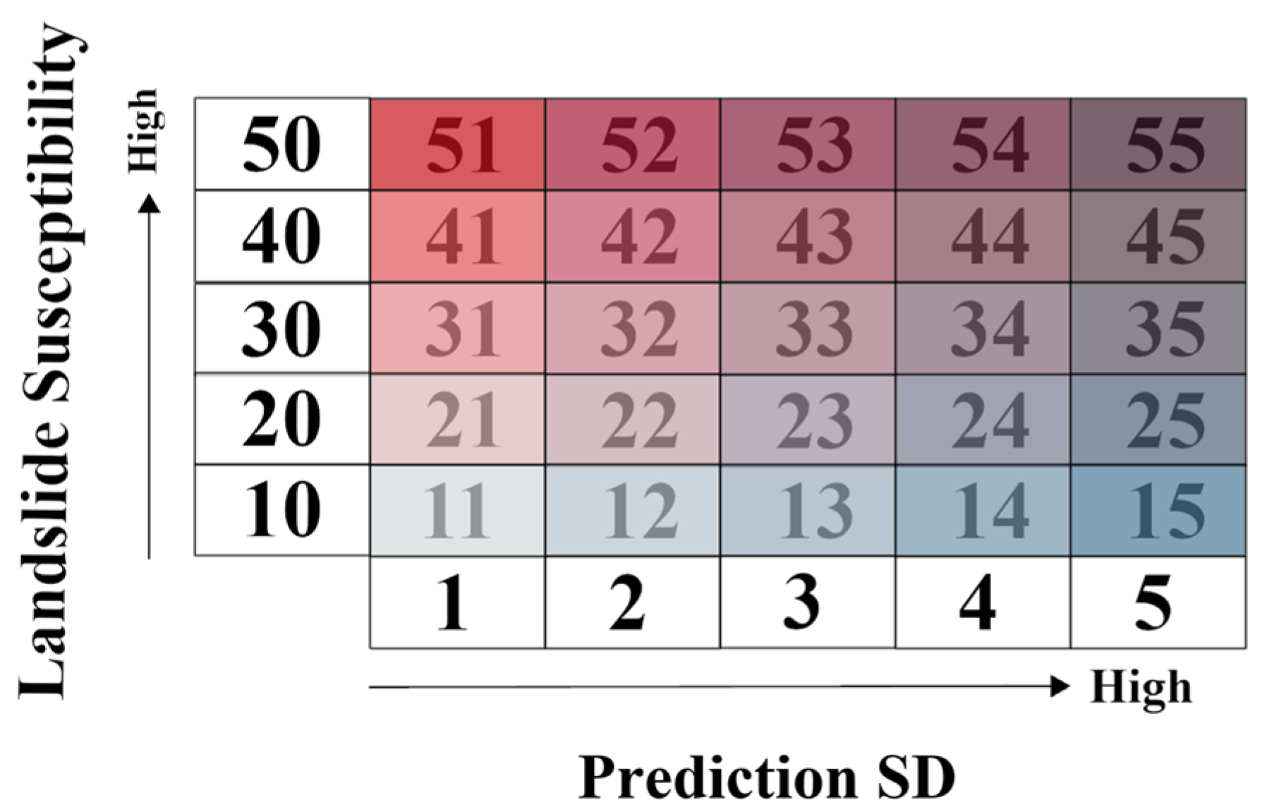
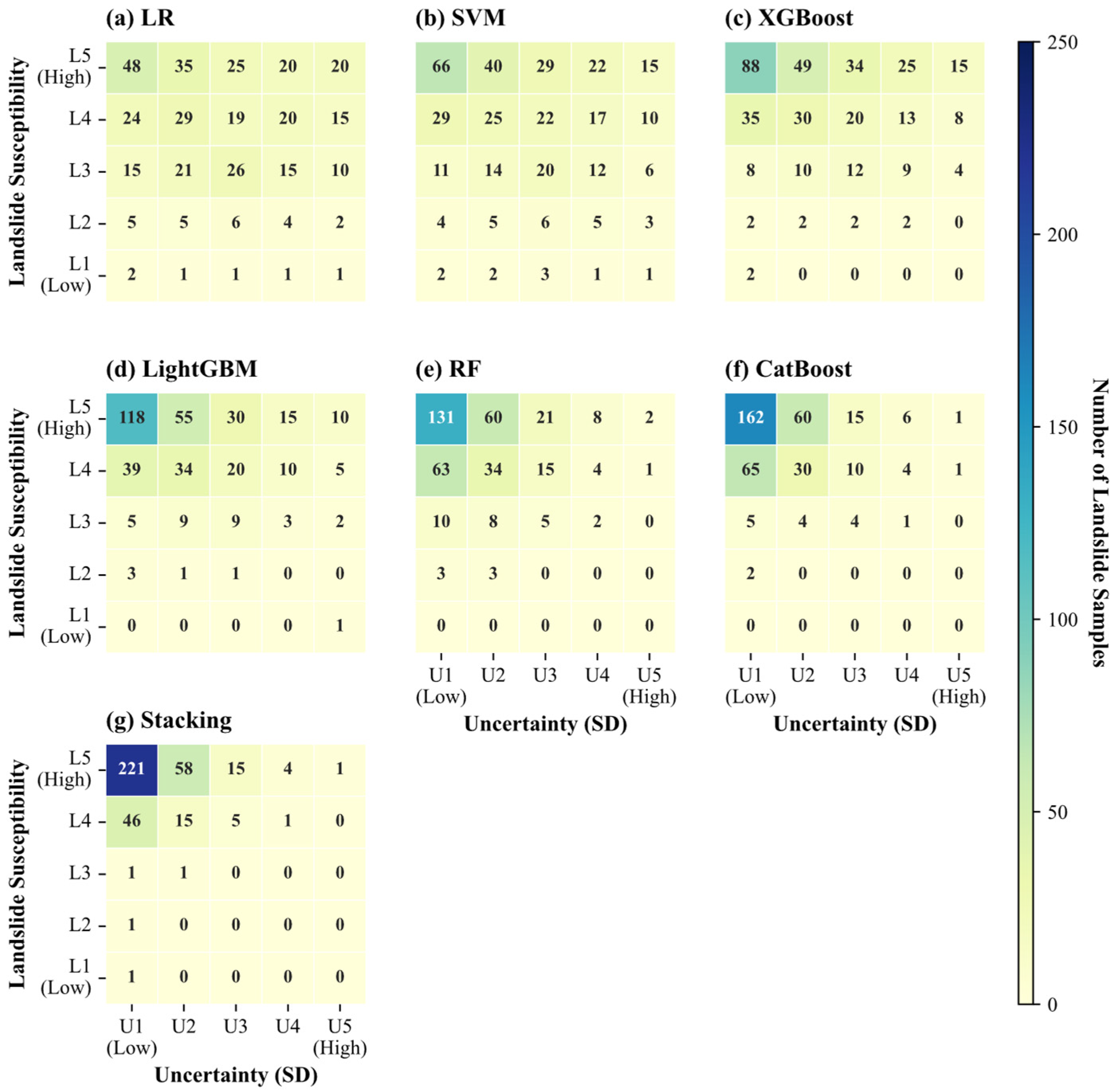
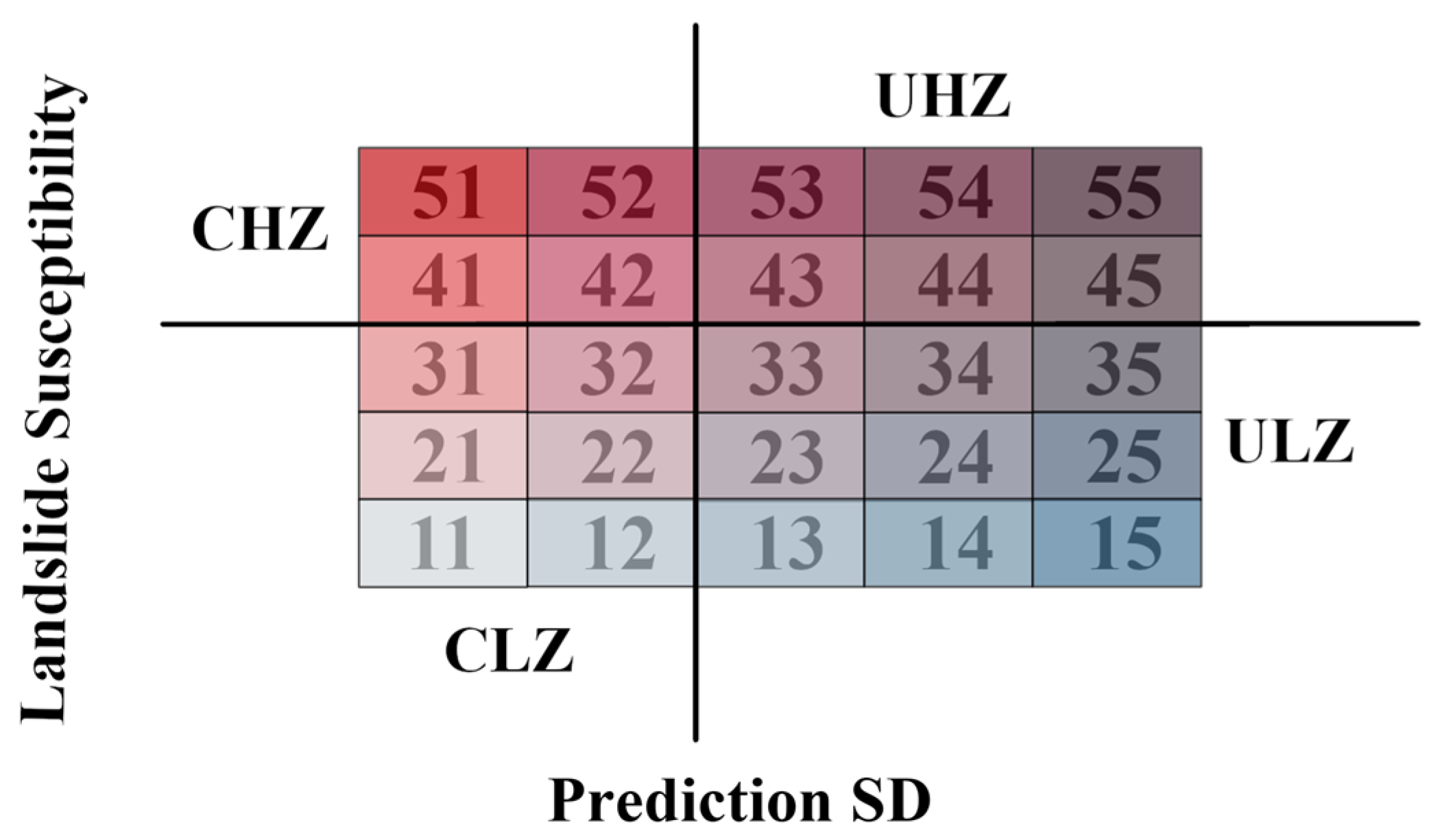
To further examine the spatial relationship between susceptibility and prediction reliability, a 5 × 5 confidence matrix integrating susceptibility and uncertainty levels was constructed (Figure 9). The matrix defines susceptibility classes (L1–L5) along the vertical axis and uncertainty classes (U1–U5) along the horizontal axis. Within this framework, the L5U1 category represents areas of both high susceptibility and low uncertainty, and can thus be interpreted as a spatially stable susceptibility core.

Because the susceptibility classes were defined using model-specific Jenks breaks, individual L–U cells were not treated as equivalent categories across models. However, the uncertainty levels were defined using common SD thresholds, allowing direct comparison of the column-wise uncertainty distributions. The LR and SVM matrices showed broader distributions of landslide samples across the uncertainty levels, whereas 270 of the 370 landslides (72.97%) in the Stacking model occurred within U1, consistent with its lower median SD and larger low-uncertainty area proportion (Figure 10).

Within the Stacking matrix, 221 of 370 landslides (59.73%) occurred in L5–U1, indicating concentration in high-susceptibility, low-uncertainty areas. CatBoost had the lowest Brier score (0.086) and log loss (0.291), whereas Stacking showed the highest observed LOTO-CV AUC and the lowest ECE (0.042), indicating strong discrimination and comparatively stable predictions but not uniformly superior probabilistic accuracy.

Across the alternative settings, spatial agreement ranged from 76.9% to 100.0%, Cohen’s kappa from 0.742 to 1.000, and the L5–U1 Jaccard index from 0.801 to 1.000 (

Table 6. Sensitivity analysis of the Stacking confidence matrix.

Scheme	Spatial Agreement	Cohen’s Kappa	Jaccard Index for L5–U1	Landslides in L5–U1
Baseline	100.0%	1.000	1.000	221 (59.73%)
P90 truncation	94.6%	0.927	1.000	221 (59.73%)
No truncation	100.0%	1.000	1.000	221 (59.73%)
Narrow SD intervals	86.8%	0.821	0.862	213 (57.57%)
Wide SD intervals	89.4%	0.846	0.883	226 (61.08%)
Jenks uncertainty classes	76.9%	0.742	0.801	208 (56.22%)
Equal-interval susceptibility classes	82.6%	0.795	0.824	214 (57.84%)

). The proportion of landslides in L5–U1 remained between 56.22% and 61.08%, indicating that the principal confidence pattern was robust to the tested settings.

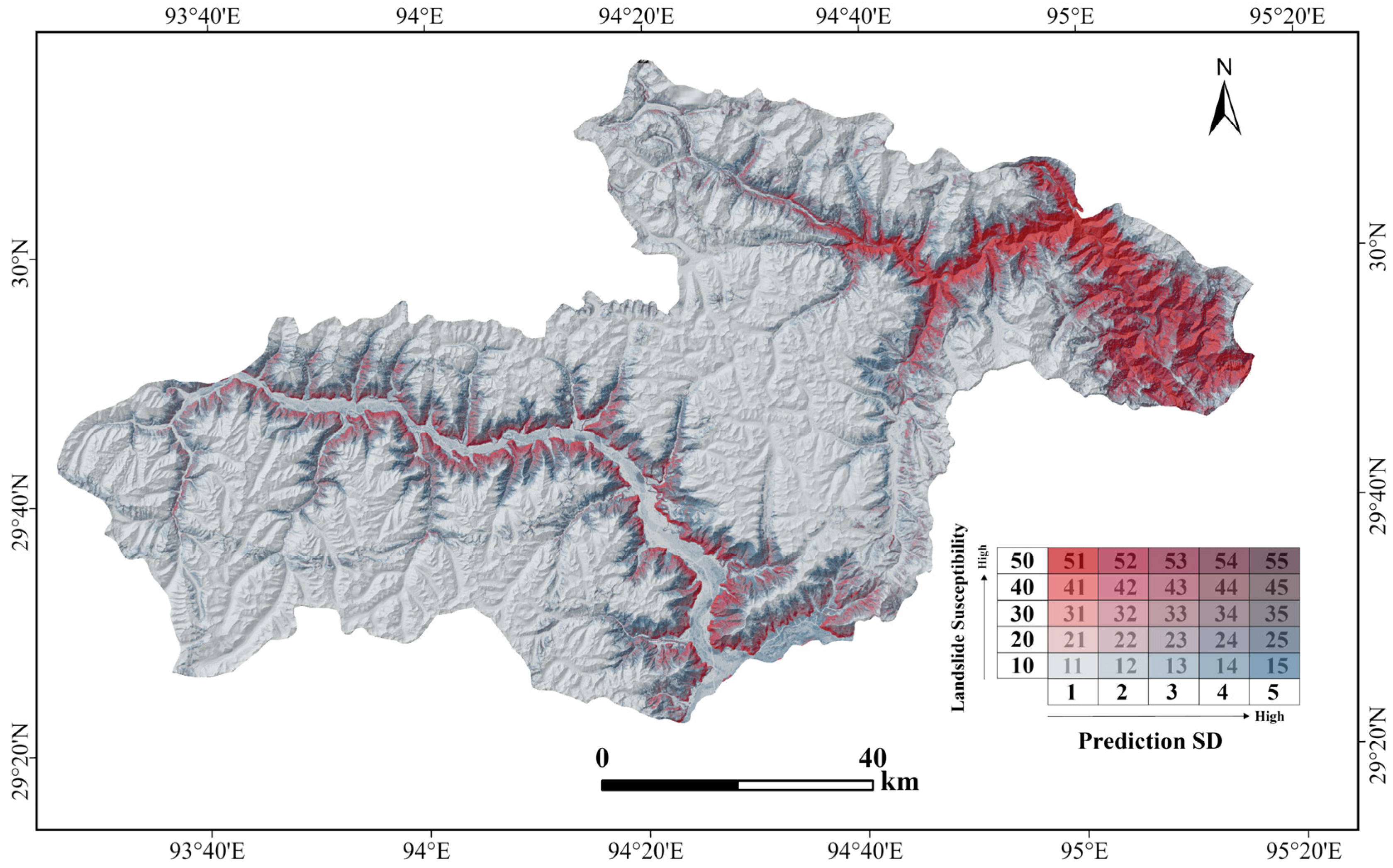
To further visualize the spatial relationship between susceptibility and uncertainty, the susceptibility and uncertainty rasters of the Stacking model were integrated pixel by pixel to generate a confidence map for the entire study area (Figure 11). The resulting map reflects the spatial organization of confidence-conditioned susceptibility patterns and provides a spatial representation of prediction reliability under repeated resampling.

3.4. Factor Contribution and Model Interpretability

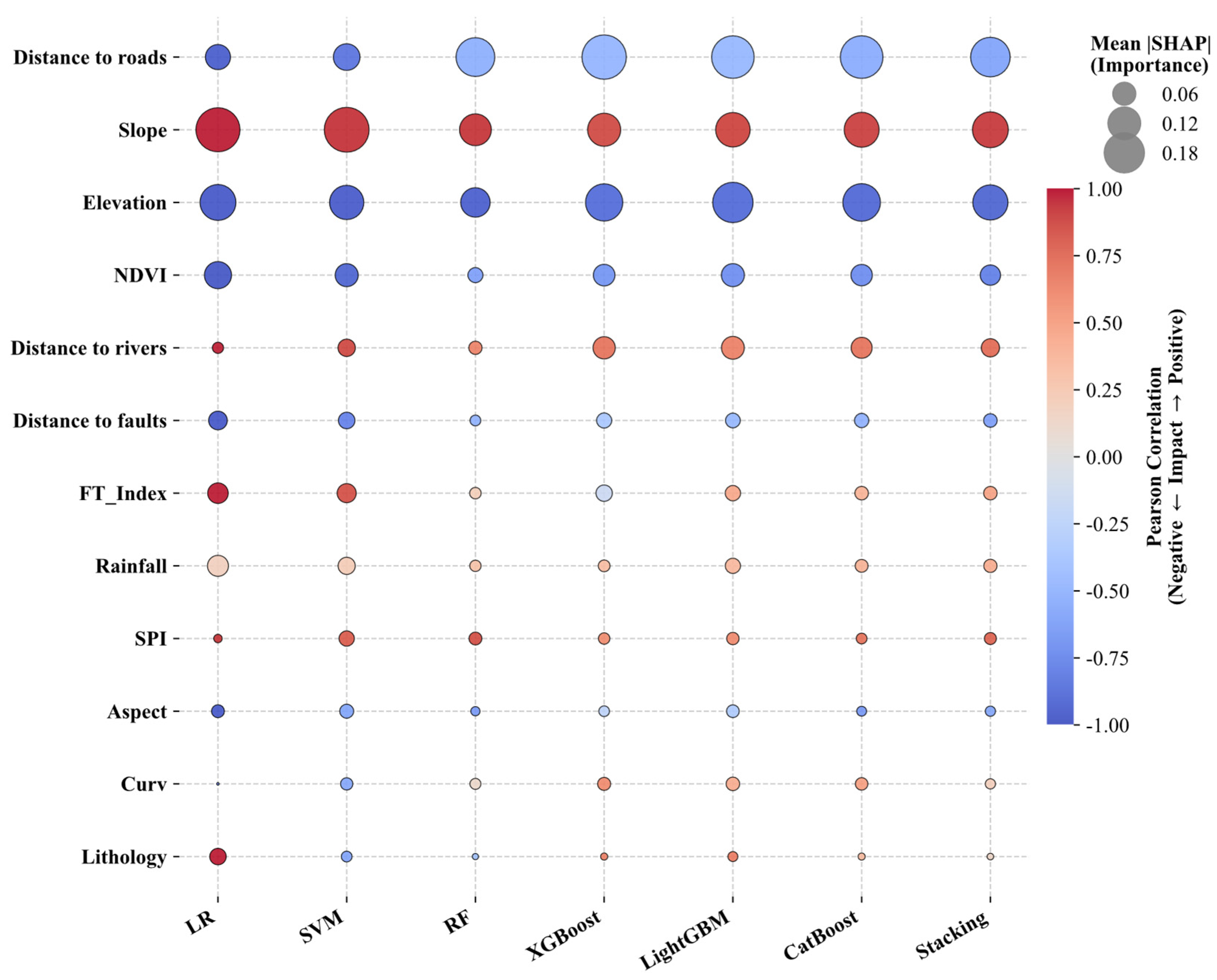
Global feature importance was quantified using the mean absolute SHAP values calculated from the test samples of all seven models. Pearson correlation coefficients between feature values and their corresponding SHAP values were used to summarize the direction of model responses.

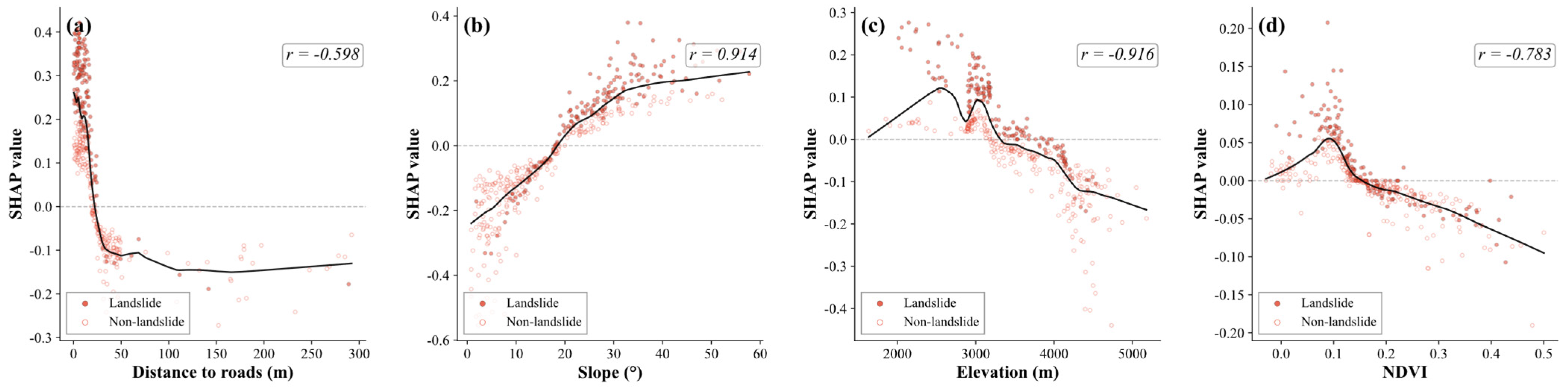
Figure 12 shows that distance to roads, slope, and elevation were consistently among the most influential conditioning factors across the individual models and the Stacking ensemble. In the Stacking model, distance to roads had the highest importance score (0.172), followed by slope (0.142) and elevation (0.136). Distance to roads and elevation were negatively associated with SHAP values, with Pearson correlation coefficients of −0.598 and −0.916, respectively, whereas slope showed a positive association, with a coefficient of 0.914. These results indicate that areas closer to roads, with steeper slopes and lower elevations, generally received higher modelled susceptibility contributions.

Figure 13 illustrates the dependence patterns of the four selected factors in the Stacking model. Distance to roads and NDVI showed negative associations with SHAP values, with Pearson correlation coefficients of −0.598 and −0.783, respectively. Slope showed a strong positive association, with a coefficient of 0.914, whereas elevation showed a pronounced negative association, with a coefficient of −0.916.

Overall, the SHAP results showed broadly consistent factor–response patterns across models. These patterns provide a model-based interpretation of the spatial susceptibility predictions.

4. Discussion

4.1. Model Performance and Factor Responses

Stacking-based ensemble models have been widely applied to landslide susceptibility mapping in mountainous regions, typically achieving high predictive performance. Chen et al. [56] reported an AUC of 0.943 using a two-layer stacking framework in a Chinese watershed, while Achu et al. [53] showed that constrained negative-sample selection can improve model performance. Wang et al. [11] observed consistent improvements over individual base learners when heterogeneous ensemble configurations were employed. In this study, Stacking achieved the highest OOB AUC (0.978) and the highest observed LOTO-CV AUC (0.922). The latter is descriptive, not statistically demonstrated; comparisons with previous studies remain cautious owing to differences in inventory size, factor selection, and validation protocols. Lv et al. [57] likewise reported that heterogeneous ensemble integration can improve the stability of model outputs, which is consistent with the relatively low resampling-based prediction uncertainty observed for the Stacking model in this study.

The performance of the Stacking model may be related to the complementary characteristics of its base learners. LR represents approximately linear relationships, SVM captures nonlinear decision boundaries in a transformed feature space, and tree-based models identify nonlinear interactions and threshold effects. Their out-of-fold predictions provide the LR meta-classifier with complementary information for ensemble weighting. The Stacking model showed the lowest mean and median prediction SD and the largest low-uncertainty area ratio among the evaluated models, indicating relatively stable predictions under repeated resampling. In contrast, prediction SD patterns differed among individual models. RF showed a comparatively narrow prediction SD range but a lower low-uncertainty area ratio, whereas SVM showed a concentrated SD distribution but only 1.58% of the study area was classified as low-uncertainty. These differences indicate that predictive accuracy and prediction stability are not necessarily equivalent across model structures.

SHAP values describe the contribution of each conditioning factor to model output within the available data distribution and should not be interpreted as direct geomechanical causation. Distance to roads, slope, and elevation were consistently identified as the dominant factors across models. In the Stacking model, shorter road distance, steeper slopes, and lower elevations were generally associated with higher susceptibility contributions. These patterns indicate associations between mapped landslide susceptibility and road proximity, terrain steepness, and valley incision in the study area.

4.2. Spatial Confidence Structure Derived from the Stacking Framework

To characterize the spatial relationship between susceptibility and prediction reliability, the 5 × 5 confidence matrix was reclassified into four confidence-conditioned susceptibility categories (Figure 14). These categories partition the study area according to both susceptibility level and uncertainty intensity, preserving susceptibility hierarchy while incorporating prediction stability into the spatial interpretation. The four-quadrant representation is a secondary interpretive aggregation of the tested 5 × 5 matrix rather than an independent analytical result.

The Confident High-Susceptibility Zone (CHZ) encompasses areas of high susceptibility and low uncertainty, representing spatially stable susceptibility cores. The Uncertain High-Susceptibility Zone (UHZ) identifies areas where high susceptibility coincides with elevated uncertainty, reflecting unstable prediction confidence under repeated resampling. The Uncertain Low-Susceptibility Zone (ULZ) corresponds primarily to transitional regions with fluctuating prediction behavior, while the Confident Low-Susceptibility Zone (CLZ) represents spatially stable low-susceptibility areas.

The spatial distribution of these categories reveals clear regional differences across Bayi District (

Table 7. Area statistics of spatial confidence decision quadrants by township in Bayi District.

Township	Total Area (km2)	CHZ		UHZ		ULZ		CLZ
		Area (km2)	%	Area (km2)	%	Area (km2)	%	Area (km2)	%
Linzhi	444.63	21.15	4.76	20.06	4.51	117.48	26.42	285.94	64.31
Bujiu	505.59	14.00	2.77	19.54	3.86	173.60	34.34	298.45	59.03
Baiba	2175.05	18.98	0.87	38.23	1.76	500.45	23.01	1617.39	74.36
Lulang	3531.18	465.22	13.17	172.63	4.89	909.57	25.76	1983.76	56.18
Bayi	1296.95	30.85	2.38	35.72	2.75	328.81	25.36	901.57	69.51
Gengzhang Menba	367.56	12.68	3.45	16.94	4.61	102.82	27.97	235.12	63.97
Mirui	220.22	9.58	4.35	14.84	6.74	149.38	67.83	46.42	21.08

). Lulang Town exhibits the largest CHZ proportion (13.17%), reflecting concentrated high-susceptibility patterns with relatively stable prediction confidence in deeply incised valley environments. Mirui Township, by contrast, shows a comparatively high UHZ proportion (6.74%), indicating greater prediction instability in areas of complex terrain heterogeneity. ULZ regions are distributed primarily near susceptibility transition zones, where model predictions remain sensitive to perturbations in the training data.

These patterns suggest that uncertainty is not spatially random but exhibits clear organization associated with terrain complexity, lithological transitions, and valley-margin environments. Relative to deterministic susceptibility maps, the confidence-conditioned representation provides additional information on the spatial stability of model predictions and identifies regions where susceptibility estimates warrant more cautious interpretation.

Most existing uncertainty assessments in landslide susceptibility mapping generate uncertainty maps without explicitly distinguishing confidence structures within susceptibility classes [58]. The framework presented here offers a spatially explicit representation in which susceptibility is conditioned on prediction confidence, enabling susceptibility intensity and reliability to be evaluated jointly. Although the thresholds remain partly empirical, the sensitivity analysis confirmed that the principal confidence pattern was stable under alternative settings.

4.3. Contributions and Limitations

This study contributes to ensemble-based landslide susceptibility mapping in three ways. First, it evaluates predictive performance and resampling-based prediction uncertainty within a unified heterogeneous Stacking framework. Second, the 5 × 5 confidence matrix integrates susceptibility and uncertainty information, distinguishing stable high-susceptibility zones from areas where high susceptibility is accompanied by lower prediction confidence. Third, the framework provides an interpretable application in a high-altitude canyon environment characterized by complex terrain, limited landslide samples, and intensive road construction.

Several limitations should be acknowledged. The landslide inventory is subject to accessibility constraints, with high-altitude areas distant from roads likely underrepresented. The limited performance changes after excluding distance to roads indicate that the model was not strongly dependent on this predictor; however, removing the predictor cannot eliminate the road-related accessibility bias already embedded in the inventory. The 2023 road layer represents the end-of-period network and may include roads constructed after some landslides recorded during 2018–2022. Because annually matched historical road data were unavailable, distance to roads cannot represent road conditions at the time of individual events. Its importance may therefore reflect both potential road-related slope disturbance and the greater accessibility of road-adjacent landslides during field surveys [59,60]. Its SHAP contribution should be interpreted as a regional spatial association rather than event-specific temporal or direct geological causality. Future work should incorporate historical road networks and remotely sensed landslide detection to improve temporal matching and inventory coverage. Lithology was encoded as an ordinal competence index. Although physically ordered, this representation imposes approximate interval spacing in LR and the RBF-SVM; because a one-hot alternative was not tested, sensitivity to encoding remains unquantified. Lithology-related effects are therefore interpreted only at the broad competence-gradient level.

The 12.5 m grid represents the common analysis and output grid rather than the native spatial resolution of every predictor. Consequently, fine-scale susceptibility patterns should not be interpreted as fine-scale variations in rainfall or freeze–thaw conditions. The uncertainty estimated in this study reflects only the variability among bootstrap-resampled models and does not include inventory errors, input-data uncertainty, hyperparameter uncertainty, or structural uncertainty associated with alternative model formulations.

5. Conclusions

This study developed an uncertainty-aware landslide susceptibility assessment framework for Bayi District, southeastern Tibet. A heterogeneous Stacking ensemble model was combined with 100 bootstrap-based resampling iterations, spatial validation, and SHAP interpretation. The results show that predictive accuracy and prediction stability are not interchangeable, as models with similar predictive performance can exhibit different spatial confidence structures.

Among the seven models, Stacking achieved the highest OOB AUC (0.978) and OOB F1-score (0.9315) and showed the highest observed LOTO-CV AUC (0.922). It also showed the lowest mean and median resampling-based prediction uncertainty, while 70.85% of the study area was classified as low-uncertainty. SHAP analysis consistently identified distance to roads, slope, and elevation as the dominant conditioning factors.

The 5 × 5 confidence matrix integrated susceptibility and uncertainty into a single spatial representation. Approximately 60% of the confirmed landslides were located in the high-susceptibility, low-uncertainty category of the Stacking model. This representation distinguishes stable high-susceptibility areas from locations where elevated susceptibility is associated with lower prediction confidence, providing information that is not available from susceptibility maps alone.

In the future, this framework could be extended to incorporate inventory, input-data, hyperparameter, and model-structure uncertainty, enabling a more comprehensive assessment of landslide susceptibility and prediction reliability.

References

1. Froude, M.J.; Petley, D.N. Global fatal landslide occurrence from 2004 to 2016. Nat. Hazards Earth Syst. Sci. 2018, 18, 2161–2181. [Google Scholar] [CrossRef] [Scilit]
2. Reichenbach, P.; Rossi, M.; Malamud, B.D.; Mihir, M.; Guzzetti, F. A review of statistically-based landslide susceptibility models. Earth Sci. Rev. 2018, 180, 60–91. [Google Scholar] [CrossRef] [Scilit]
3. Merghadi, A.; Yunus, A.P.; Dou, J.; Whiteley, J.; Binh, T.; Dieu Tien, B.; Avtar, R.; Abderrahmane, B. Machine learning methods for landslide susceptibility studies: A comparative overview of algorithm performance. Earth Sci. Rev. 2020, 207, 103225. [Google Scholar] [CrossRef] [Scilit]
4. Guo, Z.; Shi, Y.; Huang, F.; Fan, X.; Huang, J. Landslide susceptibility zonation method based on C5.0 decision tree and K-means cluster algorithms to improve the efficiency of risk management. Geosci. Front. 2021, 12, 101249. [Google Scholar] [CrossRef] [Scilit]
5. Cao, J.; Zhang, Z.; Wang, C.Z.; Liu, J.F.; Zhang, L.L. Susceptibility assessment of landslides triggered by earthquakes in the Western Sichuan Plateau. Catena 2019, 175, 63–76. [Google Scholar] [CrossRef] [Scilit]
6. Lee, S.; Sambath, T. Landslide susceptibility mapping in the Damrei Romel area, Cambodia using frequency ratio and logistic regression models. Environ. Geol. 2006, 50, 847–855. [Google Scholar] [CrossRef] [Scilit]
7. Sharma, P.; Chandel, V.B.S.; Kahlon, S.; Thakur, S.N. Assessing landslide susceptibility in the Upper Ravi river catchment, Himachal Pradesh, India: A comprehensive analysis using the logistic regression model. Geoenviron. Disasters 2025, 12, 26. [Google Scholar] [CrossRef] [Scilit]
8. Viet-Ha, N.; Shirzadi, A.; Shahabi, H.; Singh, S.K.; Al-Ansari, N.; Clague, J.J.; Jaafari, A.; Chen, W.; Miraki, S.; Dou, J.; et al. Shallow Landslide Susceptibility Mapping: A Comparison between Logistic Model Tree, Logistic Regression, Naive Bayes Tree, Artificial Neural Network, and Support Vector Machine Algorithms. Int. J. Environ. Res. Public Health 2020, 17, 2749. [Google Scholar] [CrossRef] [Scilit]
9. Liu, L.-L.; Duan, C.; Gao, J.-H.; Xiao, H.; Zhu, W.-Q.; Yang, C. Landslide susceptibility assessment using machine learning with a novel SHAP-based sampling strategy. Geosci. Front. 2026, 17, 102188. [Google Scholar] [CrossRef] [Scilit]
10. Mafigiri, A.; Khanan, M.F.A.; Abdullah, R.A. A review of GIS-based landslide susceptibility and hazard modeling considering the influence of topographic parameters on rainfall spatial variability. Model. Earth Syst. Environ. 2025, 11, 427. [Google Scholar] [CrossRef] [Scilit]
11. Wang, Z.; Wen, T.; Chen, N.; Tang, R. Assessment of Landslide Susceptibility Based on the Two-Layer Stacking Model-A Case Study of Jiacha County, China. Remote Sens. 2025, 17, 1177. [Google Scholar] [CrossRef] [Scilit]
12. Meng, S.; Shi, Z.; Li, G.; Peng, M.; Liu, L.; Zheng, H.; Zhou, C. A novel deep learning framework for landslide susceptibility assessment using improved deep belief networks with the intelligent optimization algorithm. Comput. Geotech. 2024, 167, 106106. [Google Scholar] [CrossRef] [Scilit]
13. An, B.; Zhang, Z.; Xiong, S.; Zhang, W.; Yi, Y.; Liu, Z.; Liu, C. Landslide Susceptibility Mapping Based on Ensemble Learning in the Jiuzhaigou Region, Sichuan, China. Remote Sens. 2024, 16, 4218. [Google Scholar] [CrossRef] [Scilit]
14. Fang, Z.; Wang, Y.; Peng, L.; Hong, H. A comparative study of heterogeneous ensemble-learning techniques for landslide susceptibility mapping. Int. J. Geogr. Inf. Sci. 2021, 35, 321–347. [Google Scholar] [CrossRef] [Scilit]
15. Zeng, T.; Wu, L.; Peduto, D.; Glade, T.; Hayakawa, Y.S.; Yin, K. Ensemble learning framework for landslide susceptibility mapping: Different basic classifier and ensemble strategy. Geosci. Front. 2023, 14, 101645. [Google Scholar] [CrossRef] [Scilit]
16. Jin, B.; Zhou, C.; Liu, S.; Zeng, T.; Caleca, F.; Zhao, Z.; Gui, L.; Zhao, B.; Samuele, S.; Yin, K.; et al. Space-time variability modelling of landslide susceptibility for strategic infrastructure under changing climate scenarios: The case study of the mega clean energy transmission network (Yangtze River Basin, China). Eng. Geol. 2026, 368, 108738. [Google Scholar] [CrossRef] [Scilit]
17. Jin, B.; Zhao, Z.; Zeng, T.; Liu, S.; Yang, H.; Zhao, B.; Yin, K.; Tofani, V.; Peduto, D. Spatiotemporal clustering for landslide hazard prediction revealed by the path-dependent perspective. J. Rock Mech. Geotech. Eng. 2026, in press. [Google Scholar] [CrossRef] [Scilit]
18. Jin, B.; Yin, K.; Zeng, T.; Liu, S.; Liu, Y.; Yang, H.; Wang, K.; Gui, L.; Zhao, B.; Tofani, V.; et al. Two-phase strategy framework for spatial prediction of landslide hazards in wide-area power linear engineering projects: The case of the China’s Renewable Energy Transmission Corridors. Eng. Appl. Artif. Intell. 2026, 176, 114822. [Google Scholar] [CrossRef] [Scilit]
19. Lundberg, S.M.; Erion, G.; Chen, H.; DeGrave, A.; Prutkin, J.M.; Nair, B.; Katz, R.; Himmelfarb, J.; Bansal, N.; Lee, S.I. From local explanations to global understanding with explainable AI for trees. Nat. Mach. Intell. 2020, 2, 56–67. [Google Scholar] [CrossRef] [Scilit] [PubMed]
20. Sun, D.; Wang, J.; Wen, H.; Ding, Y.; Mi, C. Landslide susceptibility mapping (LSM) based on different boosting and hyperparameter optimization algorithms: A case of Wanzhou District, China. J. Rock Mech. Geotech. Eng. 2024, 16, 3221–3232. [Google Scholar] [CrossRef] [Scilit]
21. Fabbri, A.G.; Patera, A. Spatial Uncertainty of Target Patterns Generated by Different Prediction Models of Landslide Susceptibility. Appl. Sci. 2021, 11, 3341. [Google Scholar] [CrossRef] [Scilit]
22. Lv, L.; Chen, T.; Liu, G.; Dou, J.; Plaza, A. A Comparative Study of Model Interpretability Considering the Decision Differentiation of Landslide Susceptibility Models. IEEE Trans. Geosci. Remote Sens. 2025, 63, 4401218. [Google Scholar] [CrossRef] [Scilit]
23. Madhu, D.; Nithya, G.K.; Sreekala, S.; Ramesh, M.V. Regional-scale landslide modeling using machine learning and GIS: A case study for Idukki district, Kerala, India. Nat. Hazards 2024, 120, 9935–9956. [Google Scholar] [CrossRef] [Scilit]
24. Shirzadi, A.; Solaimani, K.; Roshan, M.H.; Kavian, A.; Chapi, K.; Shahabi, H.; Keesstra, S.; Bin Ahmad, B.; Dieu Tien, B. Uncertainties of prediction accuracy in shallow landslide modeling: Sample size and raster resolution. Catena 2019, 178, 172–188. [Google Scholar] [CrossRef] [Scilit]
25. Gaidzik, K.; Ramírez-Herrera, M.T. The importance of input data on landslide susceptibility mapping. Sci. Rep. 2021, 11, 19334. [Google Scholar] [CrossRef] [Scilit]
26. Zhai, S.; Sun, Y.; Lei, J.; Shao, C. An improved information quantity method for non-landslide selection to enhance landslide susceptibility evaluation: A case study in Yongfeng, South China. Nat. Hazards 2025, 121, 11773–11797. [Google Scholar] [CrossRef] [Scilit]
27. He, S.; Abudikeyimu, X.; Hu, M.; Chen, K. Evaluation on landslide susceptibility based on self-organizing feature map network and random forest model:A case study of Dayu County of Jiangxi Province. Chin. J. Geol. Hazard Control 2022, 33, 132–140. [Google Scholar] [CrossRef]
28. Huang, F.M.; Zhang, J.; Zhou, C.B.; Wang, Y.H.; Huang, J.S.; Zhu, L. A deep learning algorithm using a fully connected sparse autoencoder neural network for landslide susceptibility prediction. Landslides 2020, 17, 217–229. [Google Scholar] [CrossRef] [Scilit]
29. Sun, K.; Li, Z.Q.; Wang, S.J.; Hu, R.L. A support vector machine model of landslide susceptibility mapping based on hyperparameter optimization using the Bayesian algorithm: A case study of the highways in the southern Qinghai-Tibet Plateau. Nat. Hazards 2024, 120, 11377–11398. [Google Scholar] [CrossRef] [Scilit]
30. Li, R.W.; Zhang, M.Y.; Pei, W.S.; Melnikov, A.; Zhang, Z.; Li, G.J. Risk evaluation of thaw settlement using machine learning models for the Wudaoliang-Tuotuohe region, Qinghai-Tibet Plateau. Catena 2023, 220, 106700. [Google Scholar] [CrossRef] [Scilit]
31. Zhu, A.X.; Miao, Y.; Yang, L.; Bai, S.; Liu, J.; Hong, H. Comparison of the presence-only method and presence-absence method in landslide susceptibility mapping. Catena 2018, 171, 222–233. [Google Scholar] [CrossRef] [Scilit]
32. Di Napoli, M.; Carotenuto, F.; Cevasco, A.; Confuorto, P.; Di Martire, D.; Firpo, M.; Pepe, G.; Raso, E.; Calcaterra, D. Machine learning ensemble modelling as a tool to improve landslide susceptibility mapping reliability. Landslides 2020, 17, 1897–1914. [Google Scholar] [CrossRef] [Scilit]
33. Huang, F.M.; Chen, J.W.; Liu, W.P.; Huang, J.S.; Hong, H.Y.; Chen, W. Regional rainfall-induced landslide hazard warning based on landslide susceptibility mapping and a critical rainfall threshold. Geomorphology 2022, 408, 108236. [Google Scholar] [CrossRef] [Scilit]
34. Xu, X.L.; Qiang, Y.; Li, L.; Liang, S.Y.; Chen, T.; Yang, W.J.; Tan, X.Y.; Wang, X. Dynamic coupling of TRIGRS and RAMMS models for physics-based prediction of rainfall-triggered shallow landslides: A case study of the 2023 yanghuachi landslide, Chongqing. Bull. Eng. Geol. Environ. 2025, 85, 2. [Google Scholar] [CrossRef] [Scilit]
35. Fu, Z.; Wang, F.; Dou, J.; Nam, K.; Ma, H. Enhanced Absence Sampling Technique for Data-Driven Landslide Susceptibility Mapping: A Case Study in Songyang County, China. Remote Sens. 2023, 15, 3345. [Google Scholar] [CrossRef] [Scilit]
36. Liu, S.H.; Du, J.; Yin, K.L.; Zhou, C.; Huang, C.C.; Jiang, J.; Yu, J. Regional early warning model for rainfall induced landslide based on slope unit in Chongqing, China. Eng. Geol. 2024, 333, 107464. [Google Scholar] [CrossRef] [Scilit]
37. Li, L.M.; Feng, Q.Q.; Yu, B. Research on the application of stacking ensemble learning model with negative sample constraints in landslide susceptibility assessment. Nat. Hazards 2026, 122, 148. [Google Scholar] [CrossRef] [Scilit]
38. Binh Thai, P.; Prakash, I.; Singh, S.K.; Shirzadi, A.; Shahabi, H.; Thi-Thu-Trang, T.; Dieu Tien, B. Landslide susceptibility modeling using Reduced Error Pruning Trees and different ensemble techniques: Hybrid machine learning approaches. Catena 2019, 175, 203–218. [Google Scholar] [CrossRef] [Scilit]
39. Steger, S.; Brenning, A.; Bell, R.; Glade, T. The propagation of inventory-based positional errors into statistical landslide susceptibility models. Nat. Hazards Earth Syst. Sci. 2016, 16, 2729–2745. [Google Scholar] [CrossRef] [Scilit]
40. Li, C.J.; Ma, T.H.; Sun, L.L.; Li, W.; Zheng, A.P. Application and verification of a fractal approach to landslide susceptibility mapping. Nat. Hazards 2012, 61, 169–185. [Google Scholar] [CrossRef] [Scilit]
41. Samek, W.; Montavon, G.; Lapuschkin, S.; Anders, C.J.; Muller, K.-R. Explaining Deep Neural Networks and Beyond: A Review of Methods and Applications. Proc. IEEE 2021, 109, 247–278. [Google Scholar] [CrossRef] [Scilit]
42. Zhu, Y.C.; Sun, D.L.; Wen, H.J.; Zhang, Q.; Ji, Q.; Li, C.M.; Zhou, P.G.; Zhao, J.J. Considering the effect of non-landslide sample selection on landslide susceptibility assessment. Geomat. Nat. Hazards Risk 2024, 15, 2392778. [Google Scholar] [CrossRef] [Scilit]
43. Guzzetti, F.; Gariano, S.L.; Peruccacci, S.; Brunetti, M.T.; Marchesini, I.; Rossi, M.; Melillo, M. Geographical landslide early warning systems. Earth-Sci. Rev. 2020, 200, 102973. [Google Scholar] [CrossRef] [Scilit]
44. Rossi, M.; Guzzetti, F.; Reichenbach, P.; Mondini, A.C.; Peruccacci, S. Optimal landslide susceptibility zonation based on multiple forecasts. Geomorphology 2010, 114, 129–142. [Google Scholar] [CrossRef] [Scilit]
45. Bischl, B.; Binder, M.; Lang, M.; Pielok, T.; Richter, J.; Coors, S.; Thomas, J.; Ullmann, T.; Becker, M.; Boulesteix, A.-L.; et al. Hyperparameter optimization: Foundations, algorithms, best practices, and open challenges. Wiley Interdiscip. Rev. Data Min. Knowl. Discov. 2023, 13, e1484. [Google Scholar] [CrossRef] [Scilit]
46. Kumar, C.; Walton, G.; Santi, P.; Luza, C. Random Cross-Validation Produces Biased Assessment of Machine Learning Performance in Regional Landslide Susceptibility Prediction. Remote Sens. 2025, 17, 213. [Google Scholar] [CrossRef] [Scilit]
47. Pradhan, B.; Dikshit, A.; Lee, S.R.; Kim, H. An explainable AI (XAI) model for landslide susceptibility modeling. Appl. Soft Comput. 2023, 142, 110324. [Google Scholar] [CrossRef] [Scilit]
48. Zhang, L.Z.; Ye, S.Q.; He, D.P.; Wang, L.F.; Li, W.P.; Jin, B.J.; Zeng, T.R. Examination of Landslide Susceptibility Modeling Using Ensemble Learning and Factor Engineering. Appl. Sci. 2025, 15, 6192. [Google Scholar] [CrossRef] [Scilit]
49. Khan, D.; Akram, W.; Ullah, S. Enhancing landslide susceptibility predictions with XGBoost and SHAP: A data-driven explainable AI method. Geocarto Int. 2025, 40, 2514725. [Google Scholar] [CrossRef] [Scilit]
50. Zeng, T.; Wang, L.; Zhang, Y.; Cheng, P.; Wu, F. Landslide susceptibility modeling and interpretability based on CatBoost-SHAP model. Chin. J. Geol. Hazard Control 2024, 35, 37–50. [Google Scholar] [CrossRef]
51. Huang, F.; Cao, Z.; Jiang, S.-H.; Zhou, C.; Huang, J.; Guo, Z. Landslide susceptibility prediction based on a semi-supervised multiple-layer perceptron model. Landslides 2020, 17, 2919–2930. [Google Scholar] [CrossRef] [Scilit]
52. Dou, J.; Yunus, A.P.; Dieu Tien, B.; Merghadi, A.; Sahana, M.; Zhu, Z.; Chen, C.-W.; Khosravi, K.; Yang, Y.; Binh Thai, P. Assessment of advanced random forest and decision tree algorithms for modeling rainfall-induced landslide susceptibility in the Izu-Oshima Volcanic Island, Japan. Sci. Total Environ. 2019, 662, 332–346. [Google Scholar] [CrossRef] [Scilit]
53. Achu, A.L.; Aju, C.D.; Di Napoli, M.; Prakash, P.; Gopinath, G.; Shaji, E.; Chandra, V. Machine-learning based landslide susceptibility modelling with emphasis on uncertainty analysis. Geosci. Front. 2023, 14, 101657. [Google Scholar] [CrossRef] [Scilit]
54. Youssef, A.M.; Pourghasemi, H.R. Landslide susceptibility mapping using machine learning algorithms and comparison of their performance at Abha Basin, Asir Region, Saudi Arabia. Geosci. Front. 2021, 12, 639–655. [Google Scholar] [CrossRef] [Scilit]
55. Nhu, V.H.; Mohammadi, A.; Shahabi, H.; Bin Ahmad, B.; Al-Ansari, N.; Shirzadi, A.; Clague, J.J.; Jaafari, A.; Chen, W.; Nguyen, H. Landslide Susceptibility Mapping Using Machine Learning Algorithms and Remote Sensing Data in a Tropical Environment. Int. J. Environ. Res. Public Health 2020, 17, 4933. [Google Scholar] [CrossRef] [Scilit]
56. Chen, S.J.; Pan, Y.T.; Lu, C.D.; Wang, Y.W.; Wu, M.; Pedrycz, W. Landslide spatial prediction based on cascade forest and stacking ensemble learning algorithm. Int. J. Syst. Sci. 2025, 56, 658–670. [Google Scholar] [CrossRef] [Scilit]
57. Lv, L.; Chen, T.; Dou, J.; Plaza, A. A hybrid ensemble-based deep-learning framework for landslide susceptibility mapping. Int. J. Appl. Earth Obs. Geoinf. 2022, 108, 102713. [Google Scholar] [CrossRef] [Scilit]
58. Ghorbanzadeh, O.; Blaschke, T.; Gholamnia, K.; Meena, S.R.; Tiede, D.; Aryal, J. Evaluation of Different Machine Learning Methods and Deep-Learning Convolutional Neural Networks for Landslide Detection. Remote Sens. 2019, 11, 196. [Google Scholar] [CrossRef] [Scilit]
59. Martino, S.; Bozzano, F.; Caporossi, P.; D’Angio, D.; Della Seta, M.; Esposito, C.; Fantini, A.; Fiorucci, M.; Giannini, L.M.; Iannucci, R.; et al. Impact of landslides on transportation routes during the 2016-2017 Central Italy seismic sequence. Landslides 2019, 16, 1221–1241. [Google Scholar] [CrossRef] [Scilit]
60. Fiorucci, M.; Marmoni, G.M.; Feliziani, F.; Martino, S. Evaluating completeness and consistency in earthquake-induced ground effects inventorying: Insights from the last release of the Italian CEDIT catalogue. Bull. Eng. Geol. Environ. 2026, 85, 363. [Google Scholar] [CrossRef] [Scilit]
Figure 1. Location of the study area, landslide inventory, and spatial distribution of the LOTO-CV folds.
Remotesensing 18 02891 g001
Figure 2. Distribution of landslide conditioning factors in Bayi District (a) Elevation; (b) Slope; (c) Aspect; (d) Curvature; (e) SID; (f) Rainfall; (g) Distance to River; (h) TWI; (i) SPI; (j) Lithology; (k) Distance to Fault; (l) NDVI; (m) Distance to Road; (n) Freeze–Thaw Index.
Remotesensing 18 02891 g002
Figure 3. Workflow of the study.
Remotesensing 18 02891 g003
Figure 4. Pearson correlation matrix of the selected landslide conditioning factors. The upper triangle shows the correlation coefficients, while the lower triangle uses ellipses to represent the strength and direction of the correlations.
Remotesensing 18 02891 g004
Figure 5. Calibration curves and metrics of the seven models based on pooled LOTO-CV test predictions using ten equal-frequency bins.
Remotesensing 18 02891 g005
Figure 6. Spatial distribution of landslide susceptibility derived from multiple models in Bayi District. (a) RF; (b) XGBoost; (c) LightGBM; (d) CatBoost; (e) SVM; (f) LR; (g) Stacking.
Remotesensing 18 02891 g006
Figure 7. Boxplot distributions of spatial prediction standard deviation (SD) across models.
Remotesensing 18 02891 g007
Figure 8. Spatial distribution of prediction standard deviation across 100 resampling iterations for each model: (a) RF; (b) XGBoost; (c) LightGBM; (d) CatBoost; (e) SVM; (f) LR; (g) Stacking.
Remotesensing 18 02891 g008
Figure 9. Confidence matrix for analyzing prediction SD and deriving the confidence map.
Remotesensing 18 02891 g009
Figure 10. Distribution of landslide samples in the spatial confidence matrix for multiple models.
Remotesensing 18 02891 g010
Figure 11. Confidence map of the Stacking ensemble model.
Remotesensing 18 02891 g011
Figure 12. SHAP-based attribution bubble heatmap of landslide conditioning factors across multiple models.
Remotesensing 18 02891 g012
Figure 13. SHAP Dependence Analysis of Key Conditioning Factors: (a) Distance to roads; (b) Slope; (c) Elevation; (d) NDVI.
Remotesensing 18 02891 g013
Figure 14. Spatial confidence decision quadrants.
Remotesensing 18 02891 g014