Article

Controlled Accuracy Degradation of Photogrammetric 3D City Models

1
School of Geoscience and Info-Physics, Central South University, Changsha 410083, China
2
Key Laboratory of China–ASEAN Satellite Remote Sensing Applications, Ministry of Natural Resources of the People’s Republic of China, Nanning 530221, China
3
First Surveying and Mapping Institute of Hunan Province, Changsha 410114, China
*
Author to whom correspondence should be addressed.
Remote Sens. 2026, 18(17), 2878; https://doi.org/10.3390/rs18172878
Submission received: 26 June 2026 / Revised: 17 August 2026 / Accepted: 21 August 2026 / Published: 25 August 2026
(This article belongs to the Special Issue AI-Enhanced Remote Sensing for Image Matching and 3D Reconstruction)

Highlights

What are the main findings?
  • A controlled accuracy-degradation method for photogrammetric 3D city models was developed by combining Sigmoid-based planimetric perturbation with hybrid cascaded-chaos-driven sine-wave elevation deformation, enabling independent control of horizontal and vertical geometric changes.
  • Experiments on low-rise and high-rise photogrammetric scenes produced mean planimetric displacements of 10.474 and 10.045 m and relative elevation deformations of 5.01% and 5.30%, respectively, while maintaining monotonic elevation relationships, a direction consistency close to 100%, and small spatial-shape deviations.
What are the implications of the main findings?
  • The proposed framework reduces geometric measurement capability while retaining mesh connectivity, texture correspondence, spatial continuity, and visual interpretability, supporting risk-reduced dissemination and non-measurement-oriented visualization of photogrammetric 3D city models.
  • The bounded nonlinear deformation and seed-sensitive cascaded-chaos parameter generator provide a reproducible and model-dependent approach to controlled geometric accuracy degradation.

Abstract

Photogrammetric 3D city models contain detailed planimetric and elevation information that supports urban visualization and low-altitude applications. However, the direct dissemination of high-accuracy models may expose sensitive geometric measurements. Existing protection methods mainly focus on conventional encryption, coordinate scrambling, or two-dimensional data perturbation and do not adequately balance geometric accuracy degradation with the visual usability of textured 3D meshes. This study proposes a controlled geometric deformation method that processes the planimetric and elevation components independently. In the horizontal domain, a normalized Sigmoid function generates smooth, bounded, and spatially varying coordinate displacements. In the vertical domain, a normalized deformation function combines global elevation stretching with amplitude-constrained sine-wave superposition. The sine-wave parameters are generated using a seed-sensitive hybrid cascaded chaotic system, producing reproducible but model-dependent nonlinear deformation patterns. During processing, the mesh connectivity, face indices, texture coordinates, texture images, and material relationships remain unchanged. The method was evaluated using low-rise and high-rise photogrammetric 3D scenes with different horizontal extents and elevation characteristics. Under the selected 10 m planimetric and 5% elevation settings, the mean planimetric displacements were 10.474 and 10.045 m, while the relative elevation deformations were 5.01% and 5.30%, respectively. Both datasets maintained monotonic elevation relationships and achieved 100% direction consistency. Their spatial-shape coefficients deviated from the corresponding reference values by only 0.02% and 1.33%. The results demonstrate that the proposed method provides controllable and spatially continuous geometric deformation while maintaining mesh connectivity, overall morphology, and visual interpretability. It can therefore serve as a practical pre-processing approach for the risk-reduced dissemination and non-measurement-oriented visualization of photogrammetric 3D city models.

1. Introduction

Real-scene three-dimensional (3D) models provide real-scene, three-dimensional, and dynamically updateable representations of human production, living, and ecological spaces. In China, Real-Scene 3D China has been positioned as an important new type of national infrastructure and as a strategic geospatial data resource for digital government and the digital economy [1,2]. Internationally, 3D city models have also been widely used in urban planning, disaster management, navigation, energy analysis, environmental simulation, and public decision support [3]. With the development of standard data models and web-oriented streaming formats, such as CityGML and 3D Tiles, high-resolution 3D geospatial models are increasingly becoming reusable spatial data carriers for urban-scale applications [4,5].
The rapid growth of the low-altitude economy further increases the demand for accurate 3D geospatial information. According to the Civil Aviation Administration of China, the scale of China’s low-altitude economy exceeded 500 billion yuan in 2023 and is expected to continue expanding rapidly [6]. Low-altitude activities, including unmanned aerial vehicle (UAV) logistics, low-altitude tourism, emergency response, infrastructure inspection, and urban air mobility, require detailed information on terrain, buildings, obstacles, and takeoff and landing conditions. For UAV applications, path planning and obstacle avoidance depend strongly on the spatial distribution of obstacles and the reliability of 3D environmental representations [7]. UAV photogrammetry and UAV-based 3D city modeling have therefore become important techniques for generating detailed 3D representations of urban environments [8,9].
However, the same geometric accuracy that makes real-scene 3D models valuable also creates data-security risks. A high-resolution model may expose the precise location, geometric structure, height, and surrounding environment of sensitive facilities, key infrastructure, military-related objects, or restricted areas. Once such models are directly disseminated through web platforms, public visualization systems, or low-altitude service systems, sensitive geospatial information may be unintentionally disclosed. This concern is particularly important for real-scene 3D products because users can not only view the visible appearance of an object, but also measure its position, height, shape, and neighborhood relationship from the model geometry. Thus, the risk-reduced dissemination of 3D model products requires an appropriate geometric protection or accuracy-degradation strategy that reduces sensitive geometric measurement capability while preserving sufficient visual and functional usability.
The regulatory basis for this requirement is explicit. According to the Regulations on the Scope of State Secrets in Surveying and Mapping Geographic Information issued by the Ministry of Natural Resources and the National Administration of State Secrets Protection in 2020, 3D models, point clouds, oblique images, real-scene images, and navigation electronic maps acquired outside military restricted zones and key areas may be classified as secret surveying and mapping products when the planimetric accuracy is better than or equal to 10 m, or the relative measurement accuracy of object height is better than or equal to 5%, and the continuous coverage exceeds 25 km2 [10]. These thresholds provide quantitative references for designing controlled planimetric and elevation accuracy degradation before data dissemination.
Existing studies on geospatial encryption have mainly focused on two-dimensional (2D) vector geographic data. Early and recent studies reduced the geometric precision of vector data by coordinate displacement, nonlinear transformation, or accuracy-reduction models, and some approaches further combined encryption with digital fingerprinting for traceability [11,12]. Ouyang et al. proposed a geometric accuracy reduction method to balance confidentiality and publicity of vector data, highlighting the importance of maintaining public usability while reducing sensitive positional precision [13]. These studies provide useful ideas for controlled perturbation and usability evaluation, but their target data are mainly 2D vector objects. They do not directly address the coupled planimetric-elevation structure, mesh topology, texture correspondence, and local height relationships of real-scene 3D models.
Research on 3D data security has developed along another route. Existing methods for 3D point clouds and textured models often use chaotic mapping, geometric permutation, coordinate scrambling, texture encryption, or watermarking/fingerprinting to protect transmission security, copyright, or user traceability [14,15,16]. Although these methods improve confidentiality or traceability, many are designed as encryption or watermarking schemes rather than accuracy-degradation methods. They generally aim to make data unreadable, recoverable after decryption, or robust against attacks, whereas the dissemination of photogrammetric 3D city models requires a different balance: the processed model should remain visually interpretable and geometrically valid but should no longer retain the original sensitive planimetric and elevation measurement capability. Therefore, direct random perturbation, excessive mesh deformation, and large-scale triangle flipping are unsuitable for controlled accuracy degradation.
Compared with 2D geographic data, photogrammetric 3D city models introduce three additional challenges. First, the planimetric and elevation components must be degraded under different accuracy constraints, and the two processes should be independently controllable. Second, elevation deformation must change relative height measurements without destroying the monotonic order and neighborhood structure among adjacent vertices. Third, the transformation should retain mesh connectivity, face indices, texture coordinates, and overall morphology so that the processed model remains usable for visualization and other non-measurement-oriented applications. These requirements indicate that a suitable accuracy-degradation method should be nonlinear, bounded, reproducible, seed-sensitive, and spatially continuous.
To address these challenges, this study proposes a controlled accuracy-degradation framework for photogrammetric 3D city models. The framework combines a Sigmoid-based planimetric perturbation with an elevation deformation driven by hybrid cascaded chaos and sine-wave superposition. The planimetric component introduces smooth and bounded nonuniform displacement around a prescribed target scale, while the elevation component uses normalized height deformation, amplitude-constrained sinusoidal perturbation, and a seed-sensitive chaotic parameter generator to produce a controllable relative height change. The main contributions are as follows: (1) a geometric accuracy-degradation framework is developed to control planimetric and elevation changes independently; (2) a Sigmoid-based planimetric perturbation is used to avoid simple rigid translation while maintaining spatial continuity; (3) a hybrid cascaded-chaos-driven elevation deformation is designed to increase model-dependent nonlinear variation while constraining the maximum disturbance amplitude; and (4) the processed models are evaluated in terms of planimetric displacement, elevation deformation, monotonicity, direction consistency, spatial-shape coefficient ratio, processing efficiency, and visual usability. The proposed method is intended as a pre-processing approach for risk-reduced dissemination and non-measurement-oriented visualization of photogrammetric 3D city models.

2. Related Work

2.1. Geometric Protection and Accuracy Reduction of 2D Geospatial Data

Constrained by coordinate representation methods, the early demand for geometric encryption primarily arose from the need to ensure the confidentiality and security of 2D geospatial data. The geometric encryption of 2D geospatial data primarily considers the displacement of planar coordinates and preservation of topologies through irreversible transformations [17]. Several linear and nonlinear coordinate transformations are employed predominantly in early approaches, utilizing projection or reprojection strategies for Georeferencing [18,19] and Geo-Encryption [20], however leading to vulnerability and limited obfuscation capabilities [21,22] for data protection. A fundamental limitation of these early transformation-based methods lies in the inherent tension between obfuscation strength and data usability. Linear transformations, while computationally efficient, can be readily inverted by adversaries equipped with a small set of known control points; nonlinear transformations offer greater resistance to inversion attacks but often introduce unpredictable local distortions that degrade the geometric fidelity severely. Later implementations moved beyond direct coordinate transformation, adopting alternative paradigms for geospatial data obfuscation, including frequency-domain transforms [23], chaotic sequence generations [24], coding compressions [25], etc. However, these paradigms primarily focus on obfuscating data to prevent unauthorized duplication only for the purpose of copyright protection, without designing or evaluating the approaches from the perspective of accuracy requirements.

2.2. Geometric Protection of 3D Data

With the development of technologies such as digital twins [26,27,28], smart cities [29], and new fundamental surveying and mapping [30], the value of 3D surveying data and the corresponding demand for its confidentiality protection are steadily increasing. Recent work on the transformation of 3D coordinates or textures has been widely applied to the encryption and obfuscation of 3D geospatial data [31,32]. For 3D point clouds, existing encryption approaches focus on applying transformation vectors and perturbation offsets to point coordinates [33,34], often preserving selected geometric relationships while rendering the data visually unintelligible. For textured 3D models, previous work has addressed both coordinate obfuscation and privacy-preserving texture transformation [35]. Texture obfuscation typically employs pixel-space scrambling, frequency-domain filtering, or deep feature perturbation to suppress semantically sensitive surface appearance. However, aggressive coordinate perturbation can misalign obfuscated textures with their corresponding surface patches, introducing rendering artifacts. Furthermore, the evaluation metrics for obfuscation are also mostly grounded in a privacy-protection focus, relying either on geometric stability [36] or the identifiability by 3D classification network models [37] as criteria. Several implementations have also employed distance-based metrics such as Hausdorff or Euclidean distance for evaluation [38], yet none of them have been evaluated under accuracy requirements. Moreover, most previous work on geospatial data encryption has adopted approaches that are inherently reversible, encompassing both encryption and decryption capabilities [31,39]. These studies provide useful geometric and security mechanisms, but their objectives differ from those of the present work: rather than making the model unreadable or enabling subsequent decryption, the proposed method retains visual interpretability while introducing controlled planimetric displacement and elevation deformation to reduce geometric measurement capability. Therefore, the term “encryption” is used only when referring to previous cryptographic or data-protection studies, whereas the proposed method itself is characterized as controlled geometric obfuscation and accuracy degradation.

2.3. Chaos-Based Systems for Data Perturbation

As fundamental mapping schemes in cryptography and related security domains, chaotic map systems such as Logistic and Cubic maps can be used to generate pseudorandom numbers [40,41]. However, these original mapping methods exhibit uneven density distributions, periodic windows that an adversary can exploit to narrow the key search space, and the dynamical degradation manifesting when continuous chaotic dynamics are discretized onto finite-precision hardware. Later approaches [42,43] are applied to address the mentioned dynamical degradation problem of chaotic systems under finite-precision computing. Given the effectiveness of chaotic systems in encryption tasks, chaos-based methods have been applied in surveying and GIS tasks [22,44] to generate pseudorandom encrypted coordinates, both in 2D images [45,46] and 3D models [47]. Typically for the 3D model encryptions, chaotic outputs are mapped onto vertex coordinate offsets, normal perturbations, or texture-channel substitutions, with the multidimensional state space of coupled chaotic systems naturally accommodating the higher degrees of freedom inherent to 3D geometry. In particular, cascading across multiple dimensions, between different chaotic functions [48,49], contributes significantly to enhancing encryption complexity. Cross-dimensional cascading exploits the fact that the state variables of a multi-dimensional chaotic system are coupled through their governing equations, so that perturbing one dimension propagates nonlinearly to all others. Inter-function cascading, where the output of one chaotic map serves as the seed or parameter perturbation of another, further compounds complexity by composing their distinct nonlinear characteristics. As a variant of chaotic encryption systems, cascaded chaotic systems [50,51] can significantly extend cycle length and enhance complexity, thereby counteracting dynamical degradation, which has been proven highly effective across a range of encryption tasks. Cascaded chaotic systems provide useful mechanisms for generating complex and seed-sensitive parameter sequences. In this study, however, the cascaded chaotic system is not employed as a cryptographic encryption mechanism; instead, it is used as a parameter generator for producing model-dependent nonlinear elevation-deformation patterns within the proposed controlled accuracy-degradation framework.

3. Preliminaries

The input material is an urban real-scene 3D mesh model, such as an OBJ or OSGB model, containing vertex coordinates, face indices, texture coordinates, texture images, and material files. For the i-th vertex, the original coordinate is defined as
P i = ( x i , y i , z i )
where x i and y i are planimetric coordinates and z i is the elevation coordinate. The method operates directly on model vertices. Mesh topology, face indices, texture coordinates, texture images, and material information are preserved, whereas the x i ′ , y i ′ , and z i ′ coordinates are transformed. The degradation vertex is denoted as
P i o u t = ( x i ′ , y i ′ , z i ′ )
The complete processing workflow consists of four stages. First, the input 3D model is parsed, and all vertex coordinates are extracted. Second, the x and y coordinates are transformed using a nonlinear Sigmoid perturbation to achieve planimetric accuracy degradation. Third, the z coordinate is normalized and deformed using a smooth elevation function whose sine-wave parameters are generated by a hybrid cascaded chaotic system. Finally, the modified coordinates are written back into the original mesh structure, while faces, UV coordinates, textures, and materials remain unchanged.

4. Materials and Methods

This section describes a controlled accuracy-degradation method for photogram-metric 3D city models. The method combines a Sigmoid-based planimetric perturbation with an elevation deformation driven by a hybrid cascaded chaotic sequence and sine-wave superposition. Before processing, the coordinate extrema are collected from all input model files in the selected folder, rather than being estimated separately for each file or tile. The same global bounds, planimetric deformation parameters, and elevation-deformation functions are then applied to every file. Therefore, adjacent files are processed under a consistent global coordinate framework. For duplicated boundary vertices with identical original coordinates, the deterministic transformation maps them to identical processed coordinates, reducing the risk of tile-boundary discontinuities caused by independent normalization.
As illustrated in Figure 1, the proposed controlled accuracy-degradation method consists of four main stages: input data preparation, planimetric accuracy degradation, elevation accuracy degradation, and processed-model output. First, a photogrammetric 3D city model is imported while retaining its vertices, faces, and textures. In the planimetric stage, the coordinate ranges are calculated and the horizontal coordinates are normalized, after which a Sigmoid-based bounded perturbation generates smooth and nonuniform displacements. In the elevation stage, the elevation values are normalized and transformed using a nonlinear deformation function. The parameters of this function are generated by a hybrid cascaded chaotic process comprising initial setup, two chaotic systems, coupling, post-processing, and parameter output, which increases the complexity and seed sensitivity of the elevation deformation. Finally, the modified horizontal and vertical coordinates are written back into the original mesh structure, producing a processed 3D model with reduced geometric measurement capability while retaining its overall visual appearance, mesh connectivity, and texture information.
In this study, “controlled” means that the imposed geometric deformation is governed by user-defined and physically interpretable parameters. The planimetric component is controlled mainly by the target planimetric scale V x y , whereas the elevation component is controlled by the global stretching parameter k, the nonlinear amplitude-control coefficient R, and the optional post-adjustment parameters α and β .

4.1. Sigmoid-Based Planimetric Accuracy Degradation

4.1.1. Coordinate Range Statistics and Normalization

The coordinate extents x min , x max , y min , and y max are calculated globally across all model tiles before perturbation. This global range-dependent step avoids over-perturbation in small tiles and insufficient perturbation in large tiles. A Sigmoid function is then used to map the coordinate domain to a smooth and bounded perturbation domain:
G ( t ) = 1 1 + e x p ( − t )
For a coordinate direction v (where v represents x or y), the normalized Sigmoid input is defined as
a v ( v i ) = − l n ( S v + 2 d v S v − 2 d v ) + k ( v − v m i n )
k = − l n ( S v − 2 d v S v + 2 d v ) + l n ( S v + 2 d v S v − 2 d v ) v m a x − v m i n
where S v is the amplitude parameter, d v is the perturbation threshold, and k is the normalization coefficient. This construction constrains the output perturbation to a predefined interval and makes the perturbation adaptive to the spatial extent of the model tile.

4.1.2. Planimetric Perturbation Model

The planimetric coordinates are transformed according to an additive nonlinear rule:
x i ′ = x i + S x 1 + e x p [ − a x ( x i ) ]
y i ′ = y i + S y 1 + e x p [ − a y ( y i ) ] − S y 2
The x-direction perturbation is strictly positive and produces the main displacement required for planimetric degradation. The y-direction perturbation is centered around zero and therefore changes the local displacement direction, preventing the degradation model from being represented as a simple rigid translation.
In the parameter configuration used in this method, the target planimetric scale is V x y = 10 m. The parameter values are set as S x = 2 V x y , S y = V x y , d x = 0.2 V x y , and d y = 0.4 V x y . With this setting, the x-direction displacement provides the dominant shift around the target scale, while the y-direction displacement introduces auxiliary non-rigid variation. After transformation, only the x i and y i coordinates are updated in the planimetric stage; z i and all non-geometric attributes are retained.

4.2. Elevation Accuracy Degradation with Hybrid Cascaded Chaos and Sine-Wave Superposition

4.2.1. Elevation Normalization

Elevation degradation is applied to the z coordinate after planimetric degradation. Let z m i n and z m a x be the minimum and maximum elevation values of the model, respectively. The total elevation range H is
H = z m a x − z m i n
Each original elevation value is normalized to the interval [0, 1] by
t i = z i − z m i n z m a x − z m i n
This normalization allows models with different elevation ranges to be processed under the same deformation parameters and improves the stability and transferability of the method.

4.2.2. Elevation Deformation Function

The normalized elevation is transformed using the following smooth multiplicative deformation function:
Φ ( t i ) = ( 1 + k ) t i [ 1 + t i ( 1 − t i ) S ( t i ) ]
where ti ∈ [0, 1] is the normalized elevation of the i-th vertex; k is a dimensionless global slope parameter, for which (1 + k) controls the principal relative stretching of the elevation range; and S(ti) is a bounded oscillatory term. The factor ti(1 − ti) modulates only the nonlinear component and suppresses it at both normalized endpoints. The oscillatory term is defined as
S ( t i ) = ∑ j = 1 n A j   s i n ( 2 π f j t i + p j )
where n is the number of superimposed sine waves, and Aj ≥ 0, fj, and pj are the amplitude, frequency, and phase of the j-th wave, respectively. In this study, n = 2. The amplitudes control the magnitude of the nonlinear modulation, the frequencies determine the number of oscillations over the normalized elevation interval, and the phases shift the locations of the oscillations. The preliminary transformed elevation is then
z i ′ = z m i n + H Φ ( t i ) ,       H = z m a x − z m i n
where zmin and zmax are the original minimum and maximum elevations, respectively, and H = zmax − zmin is the original elevation range. Equation (10) satisfies Φ(0) = 0 and Φ(1) = 1 + k. Thus, the sine-wave modulation is suppressed at both endpoints, whereas the global elevation scaling controlled by k remains active. The nonlinear deviation from the baseline mapping (1 + k) t i is bounded as
| Φ ( t i ) − ( 1 + k ) t i | ≤ 4 ( 1 + k ) 27 A t o t a l
A t o t a l = ∑ j = 1 n A j = 4 R
The maximum of t2(1 − t) over t ∈ [0, 1] is 4/27 and |S(t)| ≤ Atotal. The total sine-wave amplitude and its relationship to the implementation parameter R are defined by Equation (14), where Atotal is the sum of the nonnegative wave amplitudes and R is a dimensionless nonlinear amplitude-control coefficient. Combining Equations (13) and (14) gives a rigorous normalized nonlinear-deviation bound of 16(1 + k)R/27. Therefore, R is an amplitude-control coefficient rather than the exact maximum deformation. With k = 0.05 and R = 0.02, Atotal = 0.08, and the nonlinear component is bounded by 0.01244H (approximately 1.24% of the original elevation range), while the principal nominal elevation change remains governed by k = 0.05. This conservative configuration was adopted to reduce the risk of local elevation-order reversal and visually disruptive surface distortion.

4.2.3. Hybrid Cascaded Chaotic Parameter Generator

The sine-wave parameters are generated by a hybrid cascaded chaotic sequence to avoid using fixed and easily fitted perturbation functions. Two maps are combined: the Logistic map and an improved Cubic map. The Logistic map is
x n + 1 = μ x n ( 1 − x n )
and the improved Cubic map is
x n + 1 = x n 3 a 2 − b x n
The Logistic–Logistic (L-L) cascaded map applies two Logistic iterations with different parameters:
x n + 1 = μ 1 [ μ 2 x n ( 1 − x n ) ] [ 1 − μ 2 x n ( 1 − x n ) ]
The Logistic–Cubic (L-C) cascaded map first applies a Logistic transformation and then an improved Cubic transformation. With a = 0.5 and b = 3, it is expressed as
x n + 1 = | [ μ 3 x n ( 1 − x n ) ] 3 0.25 − 3 μ 3 x n ( 1 − x n ) |
It should be noted that the raw output of the cascaded chaotic update is not used directly as a parameter value. After each iteration, fractional-part extraction is applied: x ← x − floor(x), which is equivalent to a modulo-one operation and constrains the normalized chaotic state to [0, 1). The initial state is processed using the same rule. If the resulting state is exactly zero, it is replaced by 10−6 to avoid a degenerate sequence.
A state-dependent dynamic switching mechanism is used to increase sequence complexity. At each iteration, the current chaotic state is converted into an N 1 -bit binary fraction, and the Hamming weight w is calculated. If w is odd, the next iteration uses the L-L cascaded map; if w is even, it uses the L-C cascaded map. The first N 2 iterations are discarded as a burn-in stage to remove transient effects. The parameter configuration used here is μ 1 = 4.0, μ 2 = 2.3, μ 3 = 2.3, N 1 = 16, N 2 = 200, and k b = 7, where k b denotes the selected binary bit position for random-bit extraction. The resulting sequence supplies random values in [0, 1) for amplitude allocation, frequency selection, and phase selection.
The sine-wave parameters are generated using Algorithm 1.
Algorithm 1: Chaotic Generation of Sine-Wave Parameters
Input: Initial value x 0 ; control parameters μ 1 , μ 2 , μ 3 ; binary precision N 1 ;
     iteration number N 2 ; scaling parameter k b ; total amplitude A t o t a l .

Output: Sine-wave parameters A 1 , A 2 , f 1 , f 2 , p 1 , and p 2 .

1. Initialize x ← x 0 − floor( x 0 ).
2. If x = 0, set x ← 10 − 6 .
3. For i = 1 to N 2 do
4.    Convert x into an N 1 -bit binary fraction.
5.    Compute the Hamming weight w of the binary sequence.
6.    If w is odd, update x using the Logistic–Logistic cascaded map.
7.    Otherwise, update x using the Logistic–Cubic cascaded map.
8.    Normalize x ← x − floor(x).
9. End for.
10. Generate six bounded pseudo-random values μ   ∈ [0, 1) from 16 extracted bits.
11. Use r 1 and r 2 to allocate A 1 and A 2 from A t o t a l , with exceptional handling
     when r 1 + r 2 < ε.
12. Set f 1 and f 2 within [5.0, 6.5], and set p 1 and p 2 within [0, 2π].
13. Return A 1 , A 2 , f 1 , f 2 , p 1 , and p 2 .

4.2.4. Sine-Wave Parameterization and Post-Processing

For the two-sine-wave case, two chaotic random numbers r 1 and r 2 in [0, 1) are used to distribute the total amplitude:
A 1 = A t o t a l r 1 r 1 + r 2
A 2 = A t o t a l − A 1
This guarantees A 1 + A 2   = A t o t a l while allowing the detailed waveform to vary with the chaotic seed. Frequency and phase are generated as
f j = 5.0 + 1.5 λ j ,   0 ≤ λ j < 1
p j = 2 π ν j ,   0 ≤ ν j < 1
Thus, f j lies in [5.0, 6.5] and p j lies in [0, 2π]. The selected frequency interval provides sufficient nonlinear fluctuation without introducing high-frequency surface roughness. After the preliminary elevation transformation, a light global linear adjustment is applied to hide the original extreme values:
z i ″ = α z i ′ + β
where z i ′ is the preliminary transformed elevation defined in Equation (12), α is a global scale factor and β is a translation factor. The recommended ranges are α ∈ [0.999, 1.001] and β ∈ [−0.001H, 0.001H]. These small adjustments modify the extrema without visibly changing the model shape, ensuring that the primary accuracy-degradation effect remains governed by the elevation deformation function.

4.3. Evaluation Metrics

4.3.1. Planimetric Accuracy

After processing, the planimetric displacement of the i -th vertex or point is
e x y , i = ( x i ′ − x i ) 2 + ( y i ′ − y i ) 2
where e x y , i is the two-dimensional displacement magnitude. The planimetric root-mean-square error reported by the program is
R x y = N − 1 ∑ i = 1 N e x y , i 2
and the maximum and minimum planimetric displacements are also recorded.

4.3.2. Elevation Accuracy

The relative elevation-change ratio is computed with respect to the global minimum elevation:
η i = ( z i o u t − z i ) / ( z i − z m i n )
where η i is set to zero when z i − z m i n ≤ ϵ . The reported relative elevation root-mean-square error is
R z = 100 N − 1 ∑ i = 1 N η i 2   %
The maximum and minimum relative elevation deformations are calculated after excluding elevations whose absolute value is smaller than 0.01 m and after excluding near-zero denominators. This filtering matches the implementation and avoids unstable ratios around the elevation reference level.

4.3.3. Mesh Direction Consistency and Spatial-Shape Coefficient Ratio for OBJ Meshes

For OBJ meshes, topological consistency is evaluated using unique mesh edges. For an edge e = ( a , b ) , the original and degradation edge vectors are u e = p b − p a and u e ′ = p b ′ − p a ′ . Their angular deviation is
α e = a r c c o s ( ( u e ⋅ u e ′ ) / ( ∥ u e ∥   ∥ u e ′ ∥ ) )
where α e is set to zero if either vector has zero length. If M is the number of unique edges and L is the number of edges satisfying α e < 15 ° , the spatial direction consistency is
P = 100 % × L / M
It should be noted that P is a threshold-based consistency ratio. A value of 100% indicates only that all evaluated mesh-edge angular deviations are smaller than the selected tolerance threshold θ0; it does not mean that all edge directions are exactly unchanged. The angular tolerance θ0 was set to 15° as a practical threshold for identifying large local edge-direction changes. This setting is motivated by mesh-quality studies in which angular measures are used to evaluate element distortion. For example, Freitag and Ollivier-Gooch [52] evaluated tetrahedral mesh quality using dihedral-angle measures and tested fixed angular thresholds including 5°, 10°, 15°, and 30°, showing that thresholds around 10–15° can provide high-quality meshes at lower computational cost. Therefore, the 15° threshold is used here as an empirical tolerance for local directional stability rather than as a universal standard for exact direction preservation.
Spatial-shape coefficient ratio is evaluated using a spatial-shape coefficient derived from the length and angular characteristics of the projected bottom boundary. Vertices within 0.01 m of the minimum elevation are projected onto the horizontal plane; if fewer than three such vertices are available, all vertices are projected and their two-dimensional convex hull is used. The boundary vertices are stored as a deterministic ordered polyline B = (b1, …, bm) with distinct endpoints, and its spatial-shape coefficient is
C ( B ) = L ( B ) D ( B ) + Θ ( B ) 2 π
where L(B) is the sum of the Euclidean lengths of all consecutive polyline segments, D(B) = ||bm − b1|| > 0 is the endpoint distance, and Θ(B) is the cumulative absolute turning angle. The same boundary-extraction and vertex-ordering rules are applied to the original and encrypted models. A spatial-shape coefficient ratio is then defined as
S m = 100 % × C ( B o r i g ) / C ( B t r a n s )
where B o r i g and B t r a n s denote the original and transformed boundaries, respectively. The range of S m is (0, +∞), and the reference value is 1, or 100% when expressed as a percentage. A value close to 100% indicates that the processed model retains a boundary length-angle coefficient close to that of the original model. Values greater or smaller than 100% indicate that the processed boundary coefficient is slightly smaller or larger than the original one, respectively. When S m = 1, the processing has produced no effective spatial-shape change. In practical applications, the spatial-morphology similarity result should therefore be evaluated according to the specific requirements of each case.

5. Results

5.1. Planimetric Accuracy-Degradation Results

The planimetric degradation experiment was conducted on a real-scene 3D OBJ model containing 708,055 vertices. The model had an elevation range from −51.530 m to 55.223 m, with a total relief of 106.753 m. Although the following analysis focuses on the x- and y-coordinate perturbations, the complete 3D model was used to examine whether the planimetric transformation retained visual appearance and spatial continuity.
As shown in Figure 2, three target planimetric deformation scales were evaluated: 5 m, 10 m, and 15 m. The 5 m setting produced only limited geometric displacement, whereas the 10 m setting provided the best balance between the intended accuracy reduction and visual usability. The 15 m setting produced larger displacement but also reduced the scene-level geometric fidelity available for visualization. A reproducibility test showed that processing the same input file five times with identical parameters produced binary-identical OBJ outputs, confirming deterministic implementation behavior.
The coordinate-offset statistics show that the proposed planimetric transformation maintained a controlled relationship with the prescribed deformation scale (Table 1). The planimetric RMSE values were 4.948 m, 9.895 m, and 14.843 m for the 5 m, 10 m, and 15 m settings, respectively. Thus, the magnitude of the coordinate perturbation increased almost linearly with the prescribed scale. For the 10 m setting, the displacement ranged from 8.000 m to 12.649 m, and the RMSE was 9.895 m, which is close to the prescribed 10 m deformation scale.
To examine local displacement heterogeneity, 10 vertices were randomly sampled from the 10 m result (Table 2). The sampled displacement distances ranged from 8.604 m to 11.114 m, and both the x- and y-direction offsets varied among vertices. The x offsets remained positive and ranged from 8.155 m to 11.114 m, whereas the y offsets varied from −3.468 m to 3.789 m. This behavior confirms that the operation was not a simple rigid translation; instead, the displacement distance and direction changed across the model while remaining within a controlled interval around the target scale.
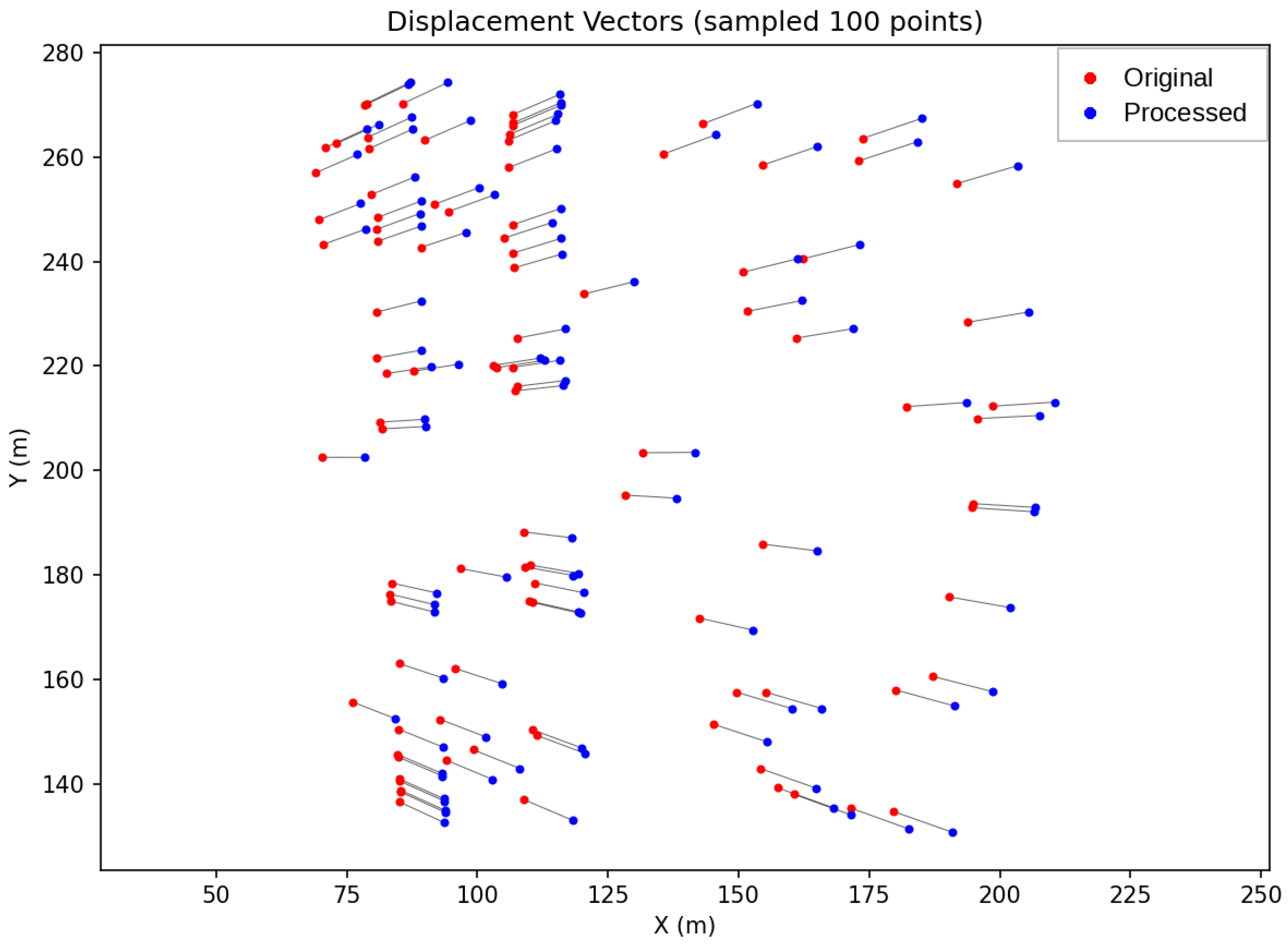
The displacement-vector visualization based on 100 sampled points further illustrates the spatial behavior of the 10 m result (Figure 3). The processed points are displaced mainly toward the upper-right and lower-right directions, but the direction and length of the vectors are not identical. At the same time, the relative arrangement of neighboring points is retained. This indicates that the Sigmoid-based planimetric deformation introduces spatially varying offsets while avoiding topological disorder or visually disruptive local displacement.
Overall, the results demonstrate that the Sigmoid-based planimetric transformation provides controllable and nonuniform coordinate perturbations. The 10 m setting most effectively balances the prescribed displacement magnitude with spatial continuity and visual interpretability. Therefore, this setting was selected for the subsequent integrated accuracy-degradation experiment.

5.2. Elevation Accuracy-Degradation Results

The elevation experiment examined how the hybrid cascaded-chaos and sine-wave transformation responded to three vertical deformation scales. As shown in Figure 4, the chaotic-system parameters were kept constant, while the global slope parameter k was set to 5.0%, 10.0%, and 15.0%. This design isolates the effect of the prescribed elevation-deformation scale on model morphology and height measurements.
When k = 5.0%, the model exhibits moderate vertical deformation while the main building morphology remains visually recognizable. When k = 10.0%, the vertical change becomes more evident, increasing the alteration of height measurements but reducing geometric fidelity. When k = 15.0%, the deformation is visually pronounced and exceeds the range preferred for public visualization; this setting is therefore used only to illustrate the transformation tolerance. Figure 4 confirms a scale-dependent response: as k increases from 5.0% to 15.0%, the vertical displacement and visual difference between the original and processed models increase progressively. The 5.0% case provides the most suitable balance between the intended elevation change and visual usability.
Figure 5 provides a quantitative explanation for the visual differences. The transformed-elevation curves deviate increasingly from the reference line as k increases, and the elevation-change profiles show larger cumulative vertical offsets under higher deformation scales. The oscillatory form of the change profiles is generated by the superimposed sine perturbation, indicating that the transformation is not a simple global height scaling. However, the increasing oscillation amplitude at higher k values also increases the risk that local relative-height relationships may become less stable. Consequently, k = 5.0% was selected as the practical elevation-deformation scale for the integrated experiment.
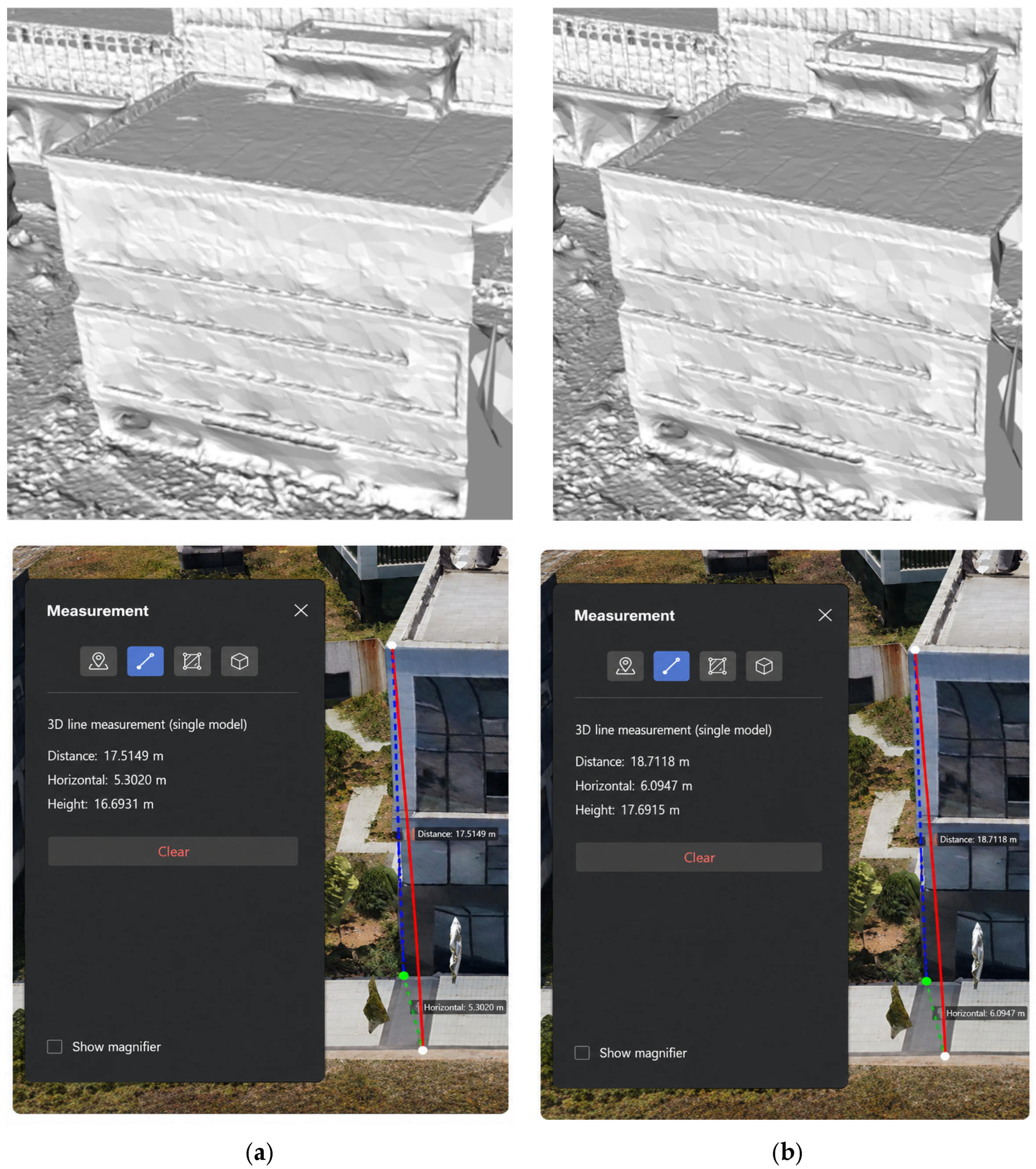
The local inspection in Figure 6 demonstrates that the 5.0% elevation transformation changes measurable height values while retaining recognizable local geometry. At the same measured position, the height difference changed from 16.9 m before processing to 17.6 m after processing, corresponding to an increase of approximately 0.7 m, or about 4.1% relative to the original measured height. This result is close to the nominal 5.0% deformation setting and indicates that relative height measurements can be modified without visually destructive local deformation.
Table 3 demonstrates the sensitivity of the hybrid cascaded-chaos parameter generator. A perturbation of the initial value at the ninth or tenth decimal place produces markedly different amplitude allocations, frequencies, and phases. This behavior enables the same algorithmic structure to generate model- and seed-dependent elevation-deformation patterns while the overall deformation magnitude remains controlled.
Table 4 evaluates the stability of the elevation transformation by measuring the monotonic-violation rate after sorting vertices by their original elevation. When R = 0.02, all tested chaotic initial values produced a monotonic-violation rate of 0.0000%, indicating that the transformed elevation sequence preserved the original relative order. At R = 0.05, several initial values began to show violations, and at R = 0.07 the violation rate reached more than 10% in some cases. These results show that the nonlinear disturbance amplitude is the key control parameter for avoiding local height-order inversion and potential triangular-facet flipping. Therefore, R = 0.02 was adopted for subsequent experiments.
Table 5 shows that the height ratio remained within a narrow range from 104.55% to 105.92% across the tested initial values. In practical terms, the transformed relative height measurement was approximately 5% greater than the original measurement, which agrees with the prescribed elevation-deformation scale. The small variation among initial values confirms that the chaotic generator changes the local deformation pattern while maintaining a controllable overall magnitude.
Table 6 verify that the elevation degradation process maintains the geometric structure of the model. Direction consistency stayed between 99.8757% and 100.0000%, and the spatial-shape coefficient ratio remained at 100.0074% for all tested seeds. The only visible fluctuation in the direction-consistency curve occurred at the initial value 0.1234568600, but the value was still higher than 99.8%. Thus, the degradation vertices preserve the local direction relationship with adjacent vertices, and the overall shape does not undergo substantial structural distortion.

5.3. Integrated Accuracy-Degradation Results for 3D Models

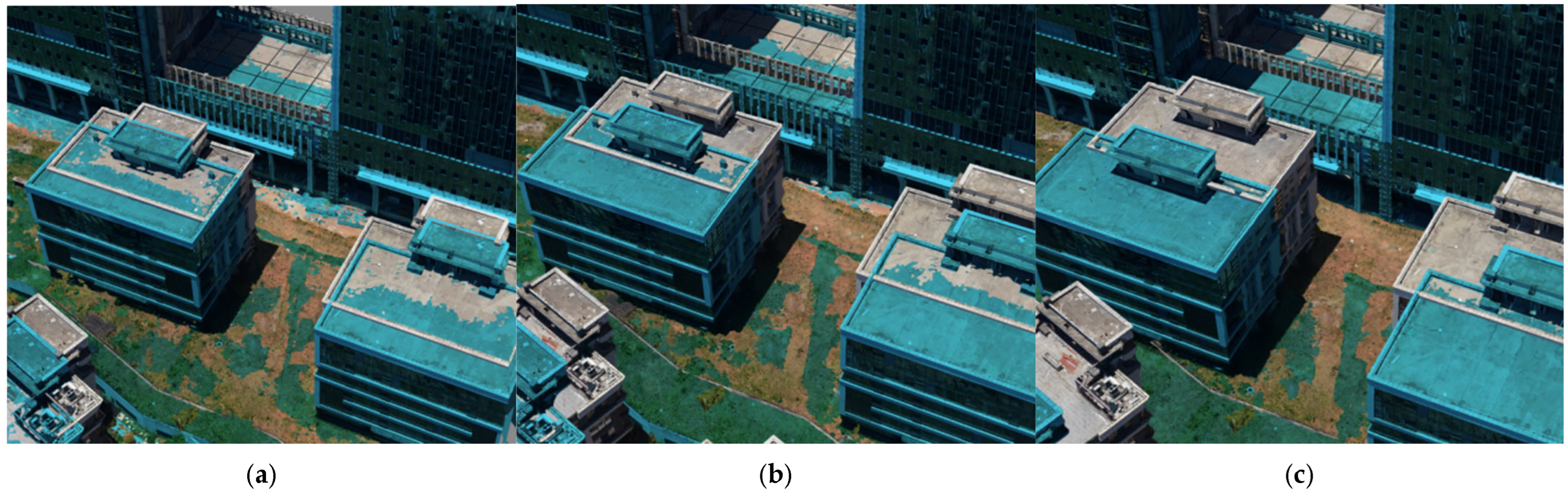
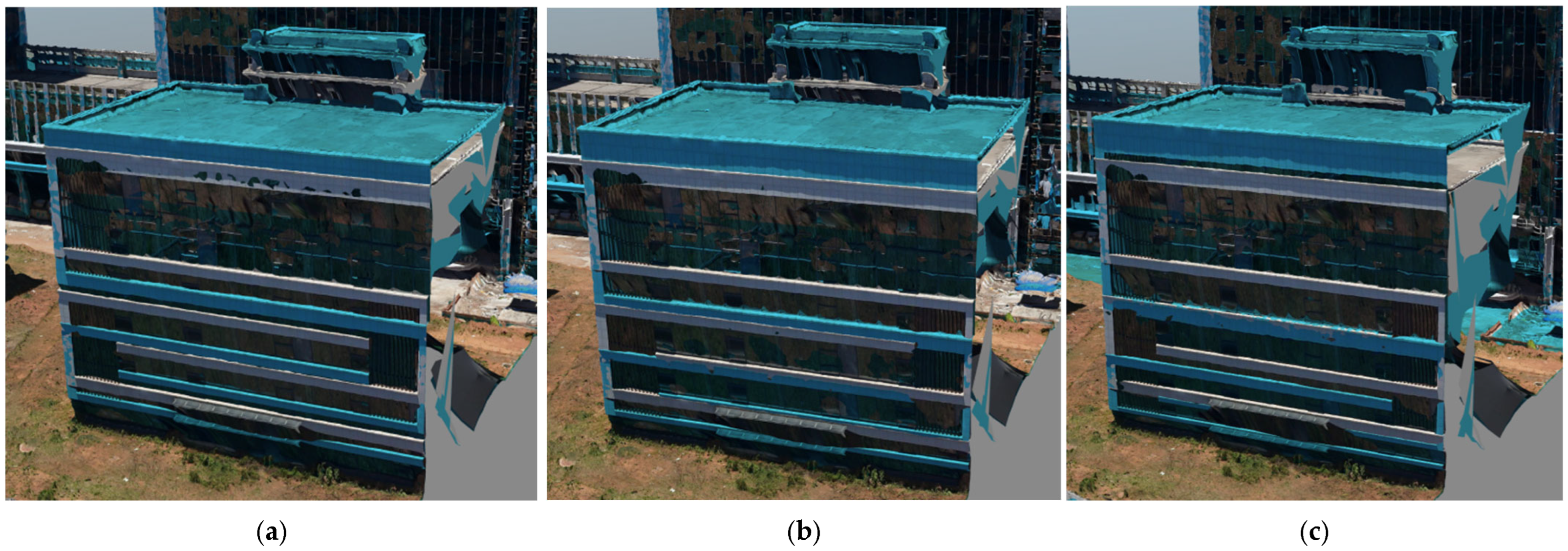
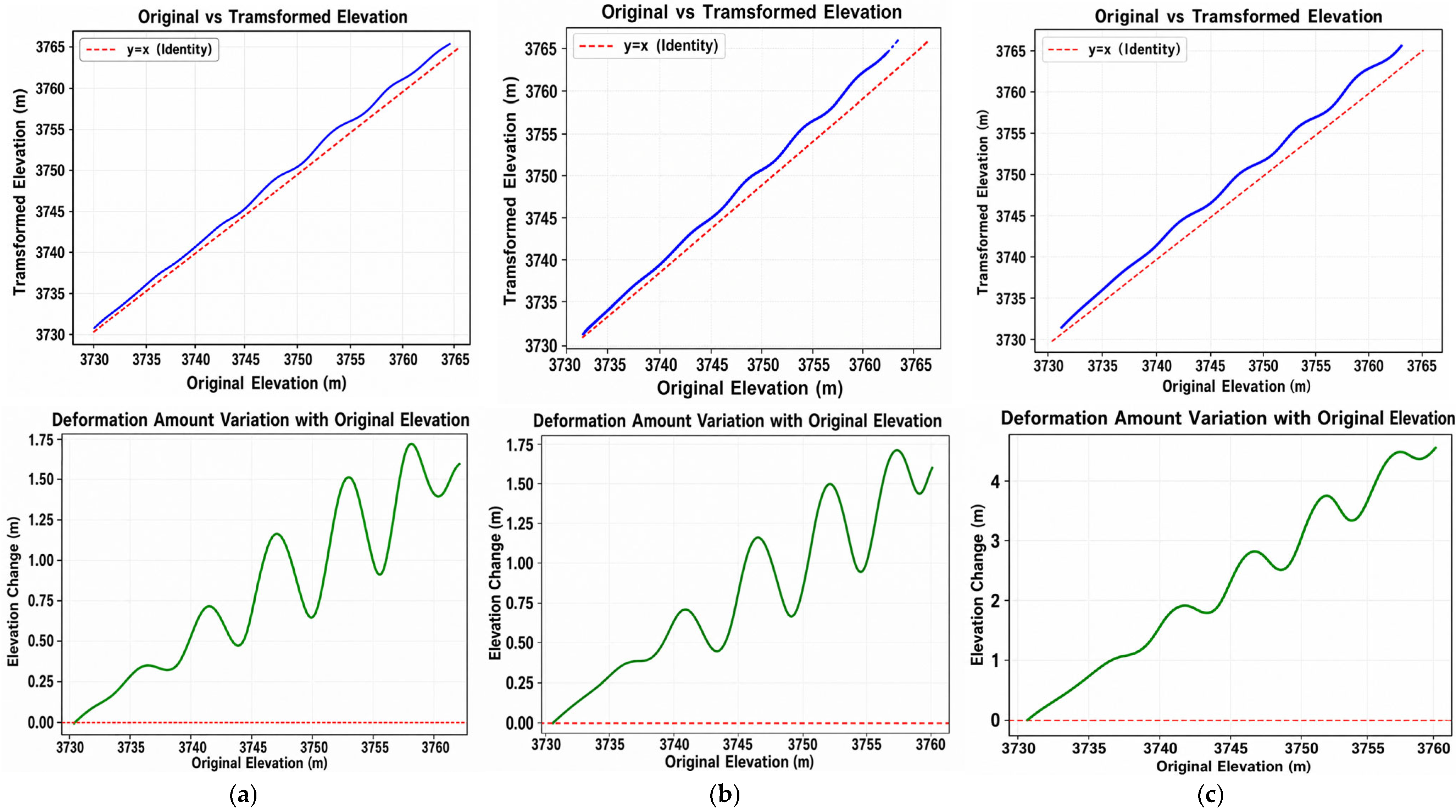
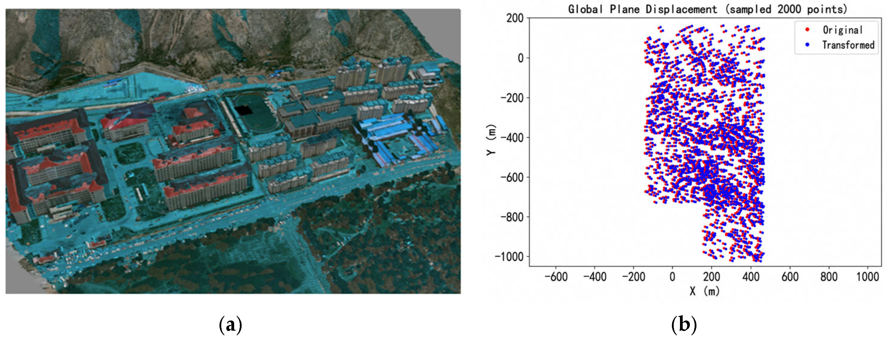
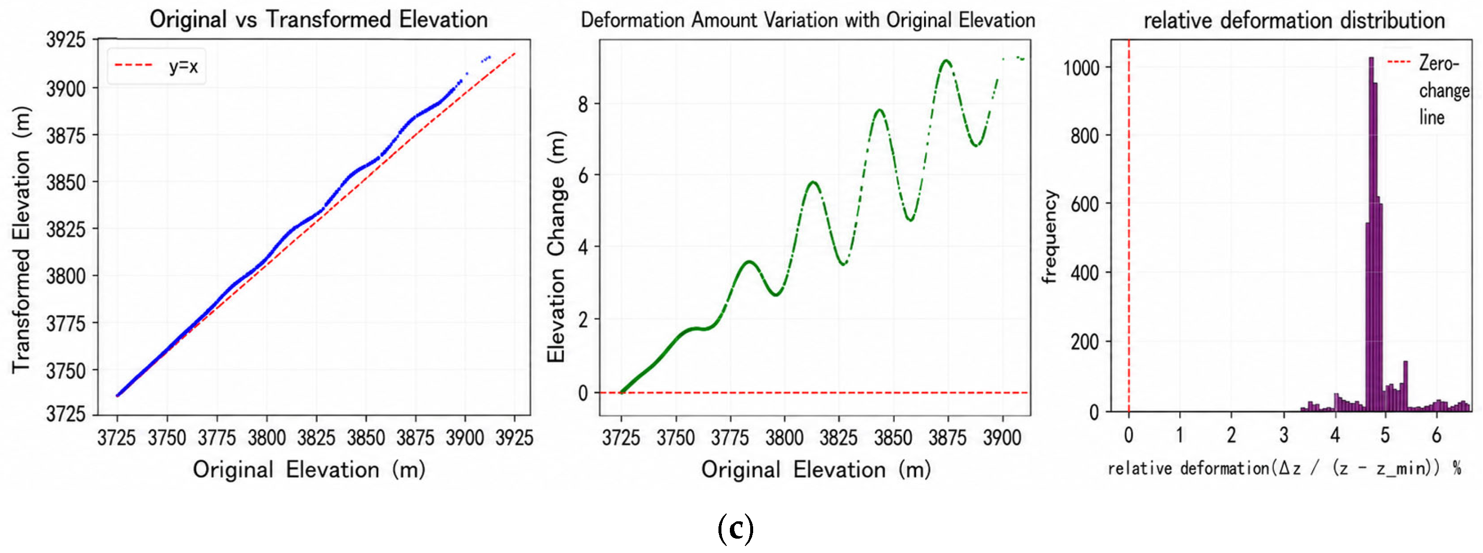
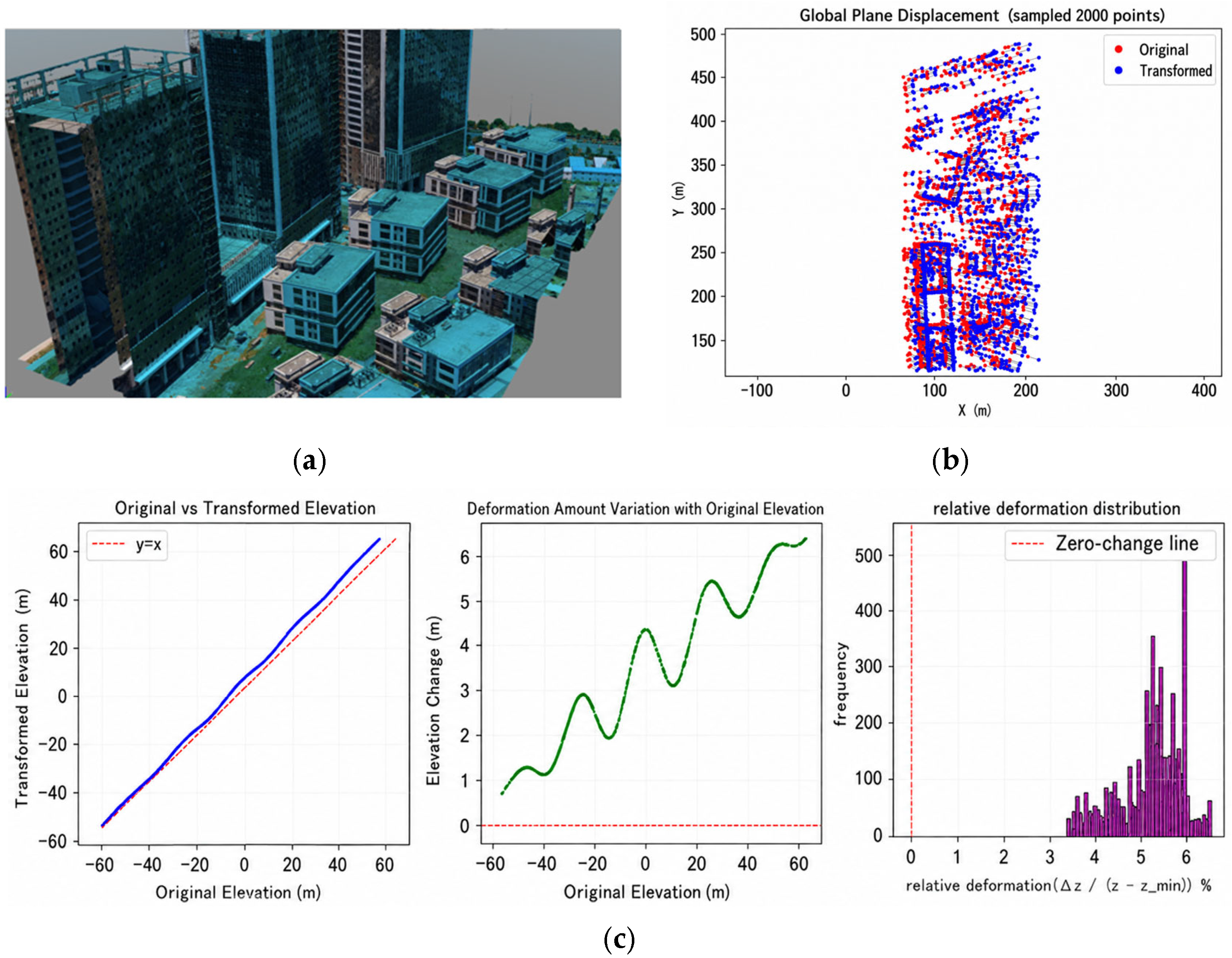
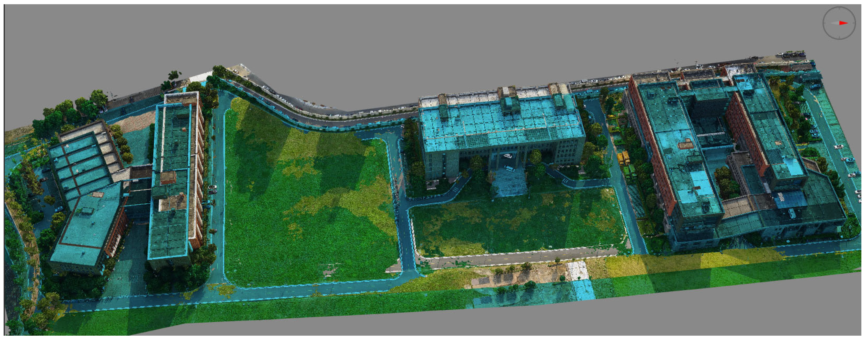
The integrated experiment combined the Sigmoid-based planimetric transformation at a target displacement scale of 10 m with the elevation transformation using a global deformation parameter of 5% and a nonlinear amplitude bound of 2%. Two photogrammetric 3D city models with different geometric characteristics were selected: a low-rise building scene with a relatively broad horizontal extent and a high-rise building scene with a compact footprint and larger vertical variation. Figure 7 and Figure 8 present the model comparison, planimetric displacement distribution, and elevation-deformation results for the two scenes.
Table 7 summarizes the parameter set used for the integrated experiment. The planimetric component was controlled at a 10 m target scale, while the elevation component used k = 0.05 and R = 0.02. The frequency, phase, chaos-control, pre-iteration, and bit-extraction settings define the model-dependent yet reproducible generation of elevation-deformation parameters. These settings were selected because the preceding results showed that they produce the prescribed deformation magnitude, avoid monotonicity violations, and retain high spatial consistency.
Figure 7 shows the integrated accuracy-degradation results for the low-rise building scene. As shown in Figure 7a, the processed model retains the overall distribution of buildings, roads, terrain, and surrounding scene elements. The principal roof outlines and relative arrangement of adjacent buildings remain visually recognizable, and no apparent gaps or discontinuities are observed. Figure 7b shows that the planimetric displacement is distributed throughout the scene rather than concentrated in a limited area. The original and processed point distributions maintain similar global patterns, indicating that the transformation changes the absolute horizontal coordinates while retaining the overall spatial organization. In Figure 7c, the transformed elevation curve deviates smoothly from the original relationship and remains globally monotonic. The corresponding elevation-change profile contains continuous oscillatory variations, demonstrating nonuniform deformation rather than constant translation or uniform vertical scaling. The deformation values remain concentrated within a limited interval across the low-rise scene.
Figure 8 presents the corresponding results for the high-rise building scene. Compared with the low-rise dataset, this scene contains taller buildings, steeper façade structures, and a more compact planimetric distribution. Figure 8a shows that the processed model retains the main building silhouettes, vertical façade structures, roof shapes, and relative positions among neighboring buildings. The high-rise structures remain visually interpretable after processing, with no obvious tearing or separation between adjacent mesh regions. Figure 8b shows an elongated planimetric point distribution corresponding to the compact and vertically dominated urban structure. Although the vertices are displaced from their original positions, the processed point set retains the principal spatial pattern of the original model, indicating that the horizontal transformation remains spatially continuous. Figure 8c shows that the elevation-transformation curve remains monotonic over the full elevation range. The nonlinear elevation-change profile varies continuously with the original elevation, and no abrupt jumps are visible. This result indicates that the method accommodates the larger vertical range of the high-rise model while maintaining a smooth elevation relationship.
A comparison of Figure 7 and Figure 8 shows that the proposed method produces similar deformation behavior in two scenes with substantially different geometric characteristics. The low-rise scene provides a broader horizontal distribution and is therefore useful for examining planimetric continuity across terrain and dispersed buildings. In contrast, the high-rise scene contains stronger elevation gradients and denser vertical structures, providing a more demanding test of elevation deformation and local mesh stability. In both cases, the main scene morphology and visual structure are retained, while the horizontal coordinates and relative elevations are measurably modified.
Figure 9 shows the integrated accuracy-degradation result for the irregular building scene (Dataset 3). Compared with the original model rendered in true surface colors, the processed model shown in blue exhibits a clear planimetric offset and vertical stretching, indicating that both horizontal and elevation accuracy were intentionally degraded.
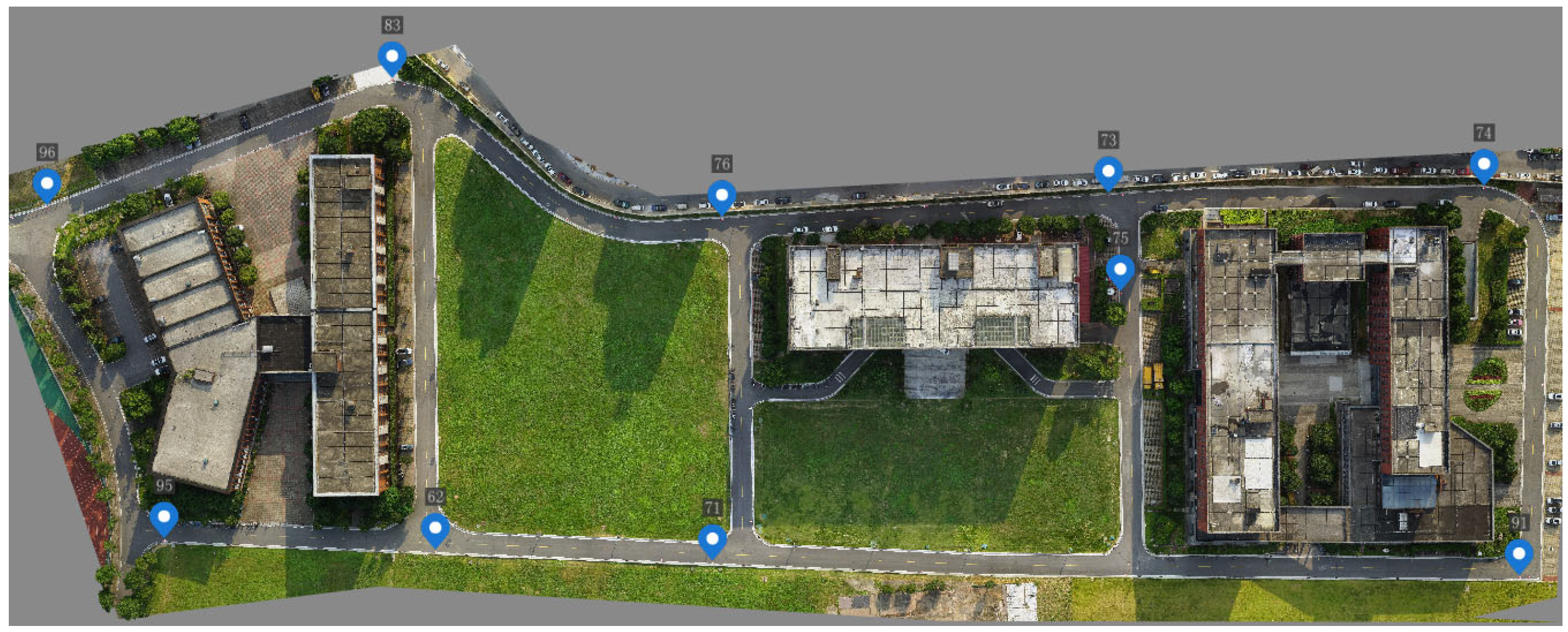
The degradation effect was further evaluated using 10 high-precision and uniformly distributed independent checkpoints (Figure 10). As shown in Table 8, the planimetric RMSE increased from 0.0250 m for the original model to 10.2387 m for the processed model, confirming that the planimetric accuracy after processing was worse than 10 m. The elevation RMSE also increased from 0.0384 m to 0.0900 m, indicating a measurable reduction in vertical accuracy. Consequently, the 3D RMSE increased from 0.0458 m to 10.2391 m, mainly due to the imposed horizontal displacement.
The object-height measurement results after elevation stretching are summarized in Table 9. The relative object-height measurement errors ranged from 4.45% to 6.15%, with an RMSE of 5.24%. This value is greater than the 5% reference threshold, confirming that the elevation stretching also reduced the relative height-measurement accuracy. Together, the visual comparison and checkpoint-based evaluation demonstrate that the integrated processing successfully degraded both planimetric and elevation accuracy while retaining the overall recognizability of the irregular building scene. Thus, the nominal 10 m planimetric translation parameter and the 5% elevation-stretching parameter are used as deformation-control settings rather than direct pointwise accuracy thresholds. Whether the processed model satisfies or fails to satisfy a given accuracy requirement should be determined through independent RMSE-based validation.
The quantitative evaluation results are summarized in Table 10. The datasets were generated from UAV oblique photogrammetry using a visible-light camera, with spatial coordinates referenced to CGCS2000. Dataset 1 represents a low-rise building scene with relatively high terrain relief, while Dataset 2 represents a high-rise building scene on relatively flat terrain. Dataset 3 was constructed by replicating a medium- to small-scale mesh model 12 times to increase the number of vertices to more than 100 million, thereby evaluating the applicability and computational performance of the proposed method on large-scale mesh data. All experiments were conducted on a laptop equipped with an Intel Core i7-10750H CPU at 2.60 GHz, 16 GB RAM, six physical cores and 12 logical processors, and an NVIDIA GeForce GTX 1650 Ti GPU with 4 GB of video memory.
The actual relative elevation deformations were 5.01%, 5.30%, and 5.05% for Datasets 1–3, respectively, which are close to the prescribed value of 5.00%. The corresponding deformation ranges were 3.38–6.60%, 3.44–6.56%, and 3.62–6.40%. The mean planimetric displacements were 10.47, 10.05, and 10.24 m, respectively, with ranges of 8.01–12.63, 8.00–12.65, and 8.00–12.65 m. These results demonstrate that both elevation and planimetric deformation magnitudes were consistently controlled around their prescribed values across the three datasets.
All three datasets achieved a direction consistency of 100.00%. The spatial-shape coefficient ratio coefficients were 100.02%, 98.67%, and 99.71% for Datasets 1–3, respectively, indicating that the overall spatial morphology was well preserved after processing. The small deviations from the reference value of 100% further demonstrate that the overall visual morphology and local edge-direction relationships of the input meshes were largely retained under the evaluated indicators.
For the evaluated dataset, the mesh-edge direction consistency reached 100.00%, with all evaluated edges showing angular deviations smaller than the 15° tolerance threshold. This value does not imply that the original and transformed edge directions were identical. The detailed angular-deviation statistics further show that the mean and median deviations were 0.9950° and 0.6324°, respectively. The 90th, 95th, and 99th percentile angular deviations were 1.6414°, 3.8232°, and 8.5964°, respectively, and the maximum angular deviation was 14.2282°. These results indicate that all evaluated edge-direction changes remained within the selected tolerance, and most mesh edges exhibited only small angular deviations after processing.
In terms of computational performance, Dataset 1 contains 668,890 vertices and requires 42.77 s for processing, while Dataset 2 contains 1,183,795 vertices and requires 69.76 s. Dataset 3 contains 130,353,583 vertices and 205,555,992 faces, with a processing time of 9109.21 s. Although Dataset 3 was artificially constructed by replicating the original mesh rather than representing an independently surveyed area, it provides a large-scale test case for evaluating the feasibility of the proposed method on meshes exceeding 100 million vertices. Overall, the results show that the proposed method maintains stable deformation magnitudes and high spatial-shape coefficient ratios across different building and terrain conditions, while remaining applicable to large-scale mesh datasets.

5.4. Baseline Comparison and Ablation Study

We conducted an ablation experiment on Dataset 1 to separately assess the contributions of the Sigmoid function, sine-wave superposition, chaotic parameter generation, and post-processing adjustment. The results are summarized in Table 11. The ablation results show that removing the Sigmoid function reduces the planimetric deformation to a uniform 10 m translation, whereas the full method produces spatially varying displacements ranging from 8.01 m to 12.63 m. Removing sine-wave superposition or chaotic parameter generation preserves the same planimetric statistics but reduces the variability of elevation-related and angular-deviation behavior. The post-processing adjustment mainly affects the final elevation values and should therefore be interpreted as an optional adjustment step rather than the dominant source of planimetric deformation. Overall, the ablation experiment confirms that the Sigmoid function contributes to nonuniform planimetric displacement, while sine-wave superposition and chaotic parameter generation contribute to controlled nonlinear elevation deformation.

6. Discussion

6.1. Effectiveness of Independently Controlled Planimetric and Elevation Deformation

The primary objective of this study was to reduce the geometric measurement capability of photogrammetric 3D city models while retaining their overall morphology, spatial continuity, and visual usability. The experimental results demonstrate that separating the planimetric and elevation components provides an effective means of controlling horizontal displacement and vertical deformation independently. Under the adopted parameter configuration, the mean planimetric displacements were 10.474 m and 10.045 m for Datasets 1 and 2, respectively, whereas the corresponding relative elevation deformations were 5.01% and 5.30%. Although the two datasets differed in vertex count, elevation range, and scene structure, their results remained close to the prescribed deformation scales. This consistency indicates that coordinate normalization reduces the influence of model size and coordinate extent and gives the method a degree of transferability across different photogrammetric models. The reported displacement and deformation values quantify the geometric changes introduced by the method; a formal product-accuracy or regulatory compliance assessment would still require independent reference data and qualified verification. Similarly, these geometric changes should not be interpreted as providing cryptographic security or formal irreversibility; they are intended to reduce the direct measurement capability of the released model.
The planimetric transformation is fundamentally different from a uniform rigid translation. The Sigmoid-based perturbation generates bounded and spatially continuous offsets according to the relative position of each vertex within the model extent. The positive displacement in the x direction provides the dominant component required to establish the overall planimetric shift, whereas the bidirectional variation in the y direction modifies the local displacement orientation. Consequently, the transformed model cannot be represented by a single constant translation vector. The continuity and boundedness of the Sigmoid function also prevent isolated vertices from receiving abrupt or excessively large offsets, thereby helping to preserve local spatial relationships and the overall projected outline of the model.
The elevation transformation likewise differs from a simple uniform vertical scaling. The global slope parameter controls the principal elevation-stretching magnitude, while the sine-wave components generated by the hybrid cascaded chaotic process introduce smooth nonlinear variations across the normalized elevation domain. The resulting transformation therefore maintains a clear global trend but produces different deformation magnitudes within different elevation intervals. Compared with a single linear scale factor, this composite deformation increases the complexity of the relationship between the original and transformed elevations while preserving a controllable overall change. The chaotic initial value mainly affects the local waveform, including the amplitude allocation, frequency, and phase, whereas the global deformation magnitude remains constrained by the slope and amplitude parameters.
The integrated experiments further indicate that the horizontal and vertical controls do not substantially interfere with one another. Adjustment of the planimetric target scale changes the horizontal displacement without modifying the elevation transformation, while adjustment of the elevation parameters changes relative height measurements without altering the prescribed planimetric perturbation. This decoupled design is useful for practical data release because the horizontal and vertical components can be configured separately according to different application requirements. It also improves parameter interpretability, as a change in one component does not require recalibration of the other component.

6.2. Preservation of Planimetric Morphology, Mesh Structure, and Visual Usability

The morphology-similarity values were 100.02% and 98.67% for Datasets 1 and 2, respectively, corresponding to deviations of only 0.02% and 1.33% from the reference value. These results indicate that the proposed planimetric deformation substantially altered the absolute coordinates while largely preserving the overall projected outlines, boundary trends, and combined length–angle characteristics of the models. This behavior can be attributed to the smooth and bounded Sigmoid transformation, which produces spatially correlated displacements rather than independent random perturbations of individual vertices.
The direction-consistency results provide complementary evidence of local geometric stability. The direction consistency ranged from 99.8757% to 100.0000% under different initial chaotic values, and both integrated datasets achieved 100%. The agreement between the morphology and direction indicators suggests that the proposed transformation preserves both the global planimetric configuration and the local direction relationships of the mesh under the selected parameters.
The nonlinear amplitude bound was also important for maintaining elevation stability. When the bound was set to 0.02, no monotonicity violations occurred for any tested chaotic initial value, indicating that the relative ordering of vertex elevations was preserved. Larger bounds of 0.05 and 0.07 produced elevation-order inversions in several cases, demonstrating that excessive nonlinear deformation may disrupt local height relationships and increase the risk of abnormal surface deformation. The selected bound therefore provides a practical balance between deformation complexity and geometric continuity.
Because the method modifies only vertex coordinates while retaining face indices, texture coordinates, texture images, and material assignments, the processed models remain directly renderable without remeshing or texture remapping. The principal building outlines, façade textures, and recognizable scene characteristics are retained, supporting their use in public visualization and other non-precision applications. Nevertheless, unchanged mesh connectivity and high consistency indicators do not constitute a complete mathematical proof of topology preservation. Although the present study reports geometry-based indicators and processing time as a function of model size, peak memory use and repeated-run statistics were not systematically recorded. Future work should include repeated-run timing, peak memory profiling, and additional visual-usability measures such as depth-map differences, silhouette overlap, or user-based evaluation. Future work should therefore include inverted-face ratios, normal deviations, edge-length distortion, local area changes, Jacobian determinants, and self-intersection tests to provide a more rigorous assessment of mesh quality.

6.3. Method Scope, Security Boundary, and Computational Scalability

It should be emphasized that the proposed method is not intended to serve as a cryptographic accuracy-degradation scheme or a formal security solution. Unlike conventional encryption methods that aim to make data unreadable without a secret key and subsequently recoverable through decryption, the proposed approach intentionally retains the visual interpretability, mesh connectivity, texture correspondence, and overall morphology of the 3D model. Its primary purpose is to reduce the direct geometric measurement capability of disseminated photogrammetric 3D city models through controlled coordinate deformation. Therefore, the method is more appropriately regarded as a controlled geometric obfuscation or accuracy-degradation approach for risk-reduced dissemination rather than as a cryptographic accuracy-degradation approach. In particular, the proposed transformation does not provide formal guarantees of irreversibility against adversaries possessing sufficient prior knowledge, original–processed point correspondences, or advanced inverse-fitting capabilities. Accordingly, its intended application is the reduction of direct measurement capability in visualization-oriented data release, rather than protection against all forms of coordinate-recovery attacks.
From a computational perspective, the dominant coordinate-transformation component operates independently on individual vertices and therefore has approximately linear computational complexity, O(N), where N is the number of vertices. In the current experiments, Dataset 1 contained 668,890 vertices and required 42.77 s, whereas Dataset 2 contained 1,183,795 vertices and required 69.76 s, showing an approximately proportional increase in processing time with model size. However, the present code prototype is designed for million-scale experimental models and retains several intermediate coordinate and mesh-analysis arrays in memory. Consequently, it should not be interpreted as a directly billion-scale implementation. For urban datasets containing hundreds of millions or billions of vertices, the coordinate transformation itself can be performed in a block-wise or streaming manner because each vertex is transformed independently, while global extrema and accuracy statistics can be accumulated online without retaining all vertices. Future implementation will therefore focus on streaming I/O, out-of-core mesh processing, parallel computation, and GPU acceleration to improve scalability for massive urban-scale datasets.
For clarity, we consider three threat-model settings. In the processed-model-only setting, the attacker has access only to the released processed model and attempts to perform direct measurement or visual interpretation. In the known-algorithm setting, the attacker knows the structure of the transformation algorithm but does not know the seed, model-dependent parameters, or exact deformation functions. In the known-point setting, the attacker additionally possesses a limited number of original-processed point correspondences or independent control points. Under these settings, plausible attack objectives include parameter fitting, spatial registration between the processed and original coordinate systems, and numerical inverse mapping. The proposed method is intended to reduce direct measurement capability under practical dissemination scenarios; it is not claimed to provide cryptographic irreversibility against all known-point or inverse-fitting attacks.
A known-point recovery experiment was conducted using four corner checkpoints, namely points 74, 91, 95, and 96, as known control points. The remaining six points were used as independent test points. Before recovery, the processed model had an XY RMSE of 10.24 m and a Z RMSE of 0.09 m relative to the true coordinates. After recovery, as shown in Table 12, the translation, affine, and quadratic polynomial models produced XY RMSE values of 2.16 m, 0.28 m, and 0.49 m, respectively. The corresponding Z RMSE values were 0.07 m, 0.05 m, and 0.05 m. Among the tested models, the affine model achieved the lowest planimetric recovery error. However, compared with the original model accuracy reported in Table 8, the recovered model still failed to reach the measurement accuracy of the original 3D model.

7. Conclusions

This study proposed a controlled accuracy-degradation method for photogrammetric 3D city models. The method integrates Sigmoid-based planimetric perturbation with elevation deformation driven by hybrid cascaded chaos and sine-wave superposition. By operating directly on vertex coordinates while retaining face indices, mesh connectivity, texture coordinates, texture images, and material relationships, the method reduces the original geometric measurement capability without destroying the visual interpretability of the model. Experimental results show that the selected 10 m planimetric setting produces displacement close to the prescribed scale and that the 5% elevation setting modifies relative height measurements while maintaining monotonic elevation relationships. The hybrid cascaded chaotic generator provides seed-sensitive, model-dependent deformation parameters, whereas the bounded nonlinear amplitude keeps the transformation controllable. Integrated tests on low-rise and high-rise photogrammetric 3D scenes further show high direction consistency and limited variation in the spatial-shape coefficient, indicating that controlled accuracy degradation can be achieved while retaining spatial continuity and visual usability. The proposed transformation should not be interpreted as a cryptographic encryption scheme; rather, it is intended as a controlled geometric obfuscation mechanism for reducing direct measurement capability while retaining visual usability. The proposed method therefore provides a practical pre-processing approach for risk-reduced dissemination and non-measurement-oriented visualization.

Author Contributions

Conceptualization, S.Z.; methodology, S.Z. and H.P.; software, Z.X., H.T. and Y.W.; validation, H.P. and Y.W.; formal analysis, S.Z.; investigation, H.T., Y.W. and S.Z.; data curation, H.T., Y.W. and S.Z.; writing—review and editing, S.Z. and Z.X.; visualization, H.T. and Z.X.; supervision, S.Z. and H.P.; funding acquisition, S.Z. and Y.W. All authors have read and agreed to the published version of the manuscript.

Funding

This research was funded by the National Natural Science Foundation of China under Grant No. 42501565; the Natural Science Foundation of Hunan Province, China, under Grant Nos. 2026JJ60405 and 2024JJ8376; the National Key R&D Program of China under Grant No. 2025YFB3910300; and the Key Laboratory of China—ASEAN Satellite Remote Sensing Applications, Ministry of Natural Resources of the People’s Republic of China, under Grant No. KLCARS-2025-G05.

Data Availability Statement

The raw data and the code of this paper will be made available by the authors on request.

Conflicts of Interest

The authors declare no conflicts of interest. The funders had no role in the design of the study; in the collection, analyses, or interpretation of data; in the writing of the manuscript; or in the decision to publish the results.

References

  1. Ministry of Natural Resources of the People’s Republic of China. Review Meeting Approved the Overall Implementation Plan for the Construction of Real-Scene 3D China (2022–2025). 2022. Available online: https://www.mnr.gov.cn/dt/ch/202207/t20220714_2742268.html (accessed on 18 June 2026).
  2. Zhang, Y.; Zou, S.; Liu, X. Sparse Point Cloud Guided Digital Surface Model Generation for Aerial Images. Geomat. Inf. Sci. Wuhan Univ. 2023, 48, 1854–1862. [Google Scholar] [CrossRef]
  3. Biljecki, F.; Stoter, J.; Ledoux, H.; Zlatanova, S.; Çöltekin, A. Applications of 3D City Models: State of the Art Review. ISPRS Int. J. Geo-Inf. 2015, 4, 2842–2889. [Google Scholar] [CrossRef] [Scilit]
  4. Open Geospatial Consortium. CityGML Standard—3D Urban Data Model and Exchange Format. Available online: https://www.ogc.org/standards/citygml/ (accessed on 18 June 2026).
  5. Open Geospatial Consortium. 3D Tiles Standard—Streaming Massive 3D Geospatial Data. Available online: https://www.ogc.org/standards/3dtiles/ (accessed on 18 June 2026).
  6. The State Council of the People’s Republic of China. China’s Low-Altitude Economy Exceeds 500 Billion Yuan: CAAC. 2024. Available online: https://english.www.gov.cn/archive/statistics/202402/28/content_WS65df262ec6d0868f4e8e46c2.html (accessed on 18 June 2026).
  7. Debnath, D.; Vanegas, F.; Sandino, J.; Hawary, A.F.; Gonzalez, F. A Review of UAV Path-Planning Algorithms and Obstacle Avoidance Methods for Remote Sensing Applications. Remote Sens. 2024, 16, 4019. [Google Scholar] [CrossRef] [Scilit]
  8. Remondino, F.; Barazzetti, L.; Nex, F.; Scaioni, M.; Sarazzi, D. UAV Photogrammetry for Mapping and 3D Modeling—Current Status and Future Perspectives. Int. Arch. Photogramm. Remote Sens. Spat. Inf. Sci. 2011, XXXVIII-1/C22, 25–31. [Google Scholar] [CrossRef] [Scilit]
  9. Hu, D.; Yang, Y.; Li, J.; Ren, G.; Wang, C.; Minner, J. UAVs and 3D City Modeling to Aid Urban Planning and Historic Preservation: A Systematic Review. Remote Sens. 2023, 15, 5507. [Google Scholar] [CrossRef] [Scilit]
  10. Ministry of Natural Resources of the People’s Republic of China; National Administration of State Secrets Protection. Regulations on the Scope of State Secrets in Surveying and Mapping Geographic Information; Natural Resources Document No. 95. 2020. Available online: https://www.fmprc.gov.cn/wjb_673085/zzjg_673183/bjhysws_674671/bhflfg/ldbjchxgfl/202303/P020230313534680395614.pdf (accessed on 18 June 2026).
  11. Wang, Y.; Yan, H.; Zhang, L. A New Declassification Method for Vector Geographic Data. In Proceedings of the 2022 International Conference on Cyber Security, Hangzhou, China, 16–18 December 2022; ACM: New York, NY, USA, 2022; pp. 58–62. [Google Scholar] [CrossRef] [Scilit]
  12. Wang, Y.; Yan, H.; Zhang, L.; Wang, X. Geometric Declassification Algorithm for Vector Geographic Data Based on Digital Fingerprint. Geogr. Geo-Inf. Sci. 2023, 39, 17–21+38. [Google Scholar] [CrossRef]
  13. Ouyang, X.; Xu, Y.; Li, B.; Liu, Y.; Wang, Z.; Yan, Y. Balance Confidentiality and Publicity of Vector Data: A Novel Geometric Accuracy Reduction Method. Int. J. Appl. Earth Obs. Geoinf. 2024, 127, 103684. [Google Scholar] [CrossRef] [Scilit]
  14. Jin, X.; Wu, Z.; Song, C.; Zhang, C.; Li, X. 3D Point Cloud Encryption Through Chaotic Mapping. In Advances in Multimedia Information Processing—PCM 2016; Lecture Notes in Computer Science; Springer: Cham, Switzerland, 2016; Volume 9918, pp. 119–129. [Google Scholar] [CrossRef] [Scilit]
  15. Jin, X.; Zhu, S.; Xiao, C.; Sun, H.; Li, X.; Zhao, G.; Ge, S. 3D Textured Model Encryption via 3D Lu Chaotic Mapping. Sci. China Inf. Sci. 2017, 60, 122107. [Google Scholar] [CrossRef] [Scilit]
  16. Liu, S.; Zhang, L.; Tan, T.; Wang, L.; Wang, P.; Zhang, Z.; Zhang, M. Homomorphic Encryption Domain Asymmetric Fingerprinting Scheme for 3D Models of Oblique Photography. Trans. GIS 2024, 28, 790–815. [Google Scholar] [CrossRef] [Scilit]
  17. Zhang, S.; Freundschuh, S.M.; Lenzer, K.; Zandbergen, P.A. The Location Swapping Method for Geomasking. Cartogr. Geogr. Inf. Sci. 2017, 44, 22–34. [Google Scholar] [CrossRef] [Scilit]
  18. White, M.S., Jr.; Griffin, P. Piecewise Linear Rubber-Sheet Map Transformation. Am. Cartogr. 1985, 12, 123–131. [Google Scholar] [CrossRef] [Scilit]
  19. Doytsher, Y. A Rubber Sheeting Algorithm for Non-Rectangular maps. Comput. Geosci. 2000, 26, 1001–1010. [Google Scholar] [CrossRef] [Scilit]
  20. Wu, F.; Cui, W.; Chen, H. A Compound Chaos-Based Encryption Algorithm for Vector Geographic Data under Network Circumstance. In Proceedings of the 2008 Congress on Image and Signal Processing; IEEE: New York, NY, USA, 2008; pp. 254–258. [Google Scholar] [CrossRef] [Scilit]
  21. Wang, M.; Wu, J.; Song, Y.; Zhang, H.; Zhu, X. A Dual-Layer Vector Map Encryption Scheme Using 4D Hyperchaos and SM4. Sci. Rep. 2026, 16, 25849. [Google Scholar] [CrossRef] [Scilit]
  22. Wang, X.; Yan, H.; Zhang, L. Vector Map Encryption Algorithm Based on Double Random Position Permutation Strategy. ISPRS Int. J. Geo-Inf. 2021, 10, 311. [Google Scholar] [CrossRef] [Scilit]
  23. Pham, N.-G.; Lee, S.-H.; Kwon, K.-R. Perceptual Encryption Based on Features of Interpolating Curve for Vector Map. IEICE Trans. Fundam. Electron. Commun. Comput. Sci. 2017, E100.A, 1156–1164. [Google Scholar] [CrossRef] [Scilit]
  24. Van, B.N.; Lee, S.-H.; Kwon, K.-R. Selective Encryption Algorithm Using Hybrid Transform for GIS Vector Map. J. Inf. Process. Syst. 2017, 13, 68–82. [Google Scholar] [CrossRef] [Scilit][Green Version]
  25. Jang, B.-J.; Lee, S.-H.; Kwon, K.-R. Perceptual Encryption with Compression for Secure Vector Map Data Processing. Digit. Signal Process. 2014, 25, 224–243. [Google Scholar] [CrossRef] [Scilit]
  26. Kustelega, M.; Mekovec, R.; Shareef, A. Privacy and Security Challenges of the Digital Twin: Systematic Literature Review. J. Univers. Comput. Sci. 2024, 30, 1782–1806. [Google Scholar] [CrossRef] [Scilit]
  27. Khan, A.; Ali, M.; Mandadi, A.; Anjum, A.; Balzter, H. Digital Twin-Ready Earth Observation: Operationalizing GeoML for Agricultural CO2 Flux Monitoring at Field Scale. Remote Sens. 2025, 17, 3615. [Google Scholar] [CrossRef] [Scilit]
  28. Chen, D.; Zhu, C.; Du, S.; Wang, Y.; Cao, Z.; Sui, M.; Kong, Y.; Feng, S.; Peethambaran, J.; Zhang, L. Structure- and Semantics-Aware Mesh Simplification for Generating Lightweight 3D Building Models. Remote Sens. 2026, 18, 914. [Google Scholar] [CrossRef] [Scilit]
  29. Barcik, P.; Coufalikova, A.; Frantis, P.; Vavra, J. The Future Possibilities and Security Challenges of City Digitalization. Smart Cities 2023, 6, 137–155. [Google Scholar] [CrossRef] [Scilit]
  30. Xue, C. Overview of the Top-Level Design and Practice of the ReS3D China. Int. Arch. Photogramm. Remote Sens. Spat. Inf. Sci. 2026, XLVIII-4/W18-2025, 337–342. [Google Scholar] [CrossRef] [Scilit]
  31. Li, S.; Zhao, R.; Guan, Q.; Chen, J.; Zhang, Y. A 3D Model Encryption Method Supporting Adaptive Visual Effects after Decryption. Adv. Eng. Inform. 2024, 59, 102319. [Google Scholar] [CrossRef] [Scilit]
  32. Priyadarsini, K.; Sivaraman, A.K.; Md, A.Q.; Malibari, A. Securing 3D Point and Mesh Fog Data Using Novel Chaotic Cat Map. Comput. Mater. Contin. 2023, 74, 6703–6717. [Google Scholar] [CrossRef] [Scilit]
  33. Usmani, M.W.; Shannigrahi, S.; Zink, M. Lightweight DRM for Volumetric Point Clouds through Attribute-Based Selective Coordinate Encryption. In Proceedings of the Twenty-sixth International Symposium on Theory, Algorithmic Foundations, and Protocol Design for Mobile Networks and Mobile Computing, MobiHoc 2025, Houston, TX, USA, 27–30 October 2025; pp. 456–461. [Google Scholar] [CrossRef] [Scilit]
  34. You, T.-Y.; Huang, Y.-T.; Hsiao, T.-Y.; Cheng, Y.-W.; Tsai, Y.-Y.; Lu, C.-T. Secure and Reversible Thumbnail-Preserving Encryption for Point Clouds via Spatial Subdivision and Chaotic Perturbation. Mathematics 2026, 14, 80. [Google Scholar] [CrossRef] [Scilit]
  35. Zhou, Q.; Ren, N.; Zhu, C.; Cai, J. A Scene-Context-Aware Texture Privacy-Preserving Method for Photogrammetric 3D Urban Models. Remote Sens. 2026, 18, 1468. [Google Scholar] [CrossRef] [Scilit]
  36. Jolfaei, A.; Wu, X.-W.; Muthukkumarasamy, V. A 3D Object Encryption Scheme Which Maintains Dimensional and Spatial Stability. IEEE Trans. Inf. Forensics Secur. 2015, 10, 409–422. [Google Scholar] [CrossRef] [Scilit]
  37. Liu, B.; Liu, Y.; Xie, Y.; Jiang, X.; Ye, Y.; Song, T.; Chai, J.; Liu, M.; Feng, M.; Yuan, H. Privacy Protection for 3D Point Cloud Classification Based on an Optical Chaotic Encryption Scheme. Opt. Express 2023, 31, 8820–8843. [Google Scholar] [CrossRef] [Scilit]
  38. Annaby, M.H.; Mahmoud, M.E.; Abdusalam, H.A.; Ayad, H.A.; Rushdi, M.A. On 3D Encryption Schemes Based on Chaotic Permutations and Rotations with Geometric Stability. Optik 2024, 300, 171680. [Google Scholar] [CrossRef] [Scilit]
  39. Jansen van Rensburg, B.; Puech, W.; Pedeboy, J.-P. A Format Compliant Encryption Method for 3D Objects Allowing Hierarchical Decryption. IEEE Trans. Multimed. 2023, 25, 7196–7207. [Google Scholar] [CrossRef] [Scilit]
  40. May, R.M. Simple Mathematical Models with Very Complicated Dynamics. Nature 1976, 261, 459–467. [Google Scholar] [CrossRef] [Scilit]
  41. Li, S.; Chen, G.; Mou, X. On the Dynamical Degradation of Digital Piecewise Linear Chaotic Maps. Int. J. Bifurc. Chaos 2005, 15, 3119–3151. [Google Scholar] [CrossRef] [Scilit]
  42. Liu, L.; Liu, B.; Hu, H.; Miao, S. Reducing the Dynamical Degradation by Bi-Coupling Digital Chaotic Maps. Int. J. Bifurc. Chaos 2018, 28, 1850059. [Google Scholar] [CrossRef] [Scilit]
  43. Alawida, M.; Samsudin, A.; Teh, J.S.; Alkhawaldeh, R.S. A New Hybrid Digital Chaotic System with Applications in Image Encryption. Signal Process. 2019, 160, 45–58. [Google Scholar] [CrossRef] [Scilit]
  44. García-Martínez, M.; Campos-Cantón, E. Pseudo-Random Bit Generator Based on Multi-Modal Maps. Nonlinear Dyn. 2015, 82, 2119–2131. [Google Scholar] [CrossRef] [Scilit]
  45. Zhang, J.; Du, J.; Xi, X.; Yang, Z. Chebyshev Chaotic Mapping and DWT-SVD-Based Dual Watermarking Scheme for Copyright and Integrity Authentication of Remote Sensing Images. Symmetry 2024, 16, 969. [Google Scholar] [CrossRef] [Scilit]
  46. Bhangale, P.; Vaikole, S. Enhanced Geospatial Raster Data Protection: Harnessing Chaos Maps and DNA Encryption. In Proceedings of the 2024 8th International Conference on Computing, Communication, Control and Automation (ICCUBEA), Pune, India, 23–24 August 2024; pp. 878–882. [Google Scholar] [CrossRef] [Scilit]
  47. Ali, N.; Rahma, A.M.; Shaker, S.H. 3D Polygon Mesh Encryption Based on 3D Lorenz Chaotic Map. Int. J. Interact. Mob. Technol. IJIM 2021, 15, 103–114. [Google Scholar] [CrossRef] [Scilit]
  48. Zhang, G.; Ding, W.; Li, L. Image Encryption Algorithm Based on Tent Delay-Sine Cascade with Logistic Map. Symmetry 2020, 12, 355. [Google Scholar] [CrossRef] [Scilit]
  49. Zheng, J.; Bao, T. An Image Encryption Algorithm Using Cascade Chaotic Map and S-Box. Entropy 2022, 24, 1827. [Google Scholar] [CrossRef] [Scilit]
  50. Zhou, Y.; Hua, Z.; Pun, C.-M.; Chen, C.L.P. Cascade Chaotic System With Applications. IEEE Trans. Cybern. 2015, 45, 2001–2012. [Google Scholar] [CrossRef] [Scilit]
  51. Agarwal, S. Designing a Pseudo-Random Bit Generator Using Generalized Cascade Fractal Function. Chaos Theory Appl. 2021, 3, 11–19. [Google Scholar] [CrossRef] [Scilit]
  52. Freitag, L.A.; Ollivier-Gooch, C. Tetrahedral Mesh Improvement Using Swapping and Smoothing. Int. J. Numer. Methods Eng. 1997, 40, 3979–4002. [Google Scholar] [CrossRef] [Scilit]
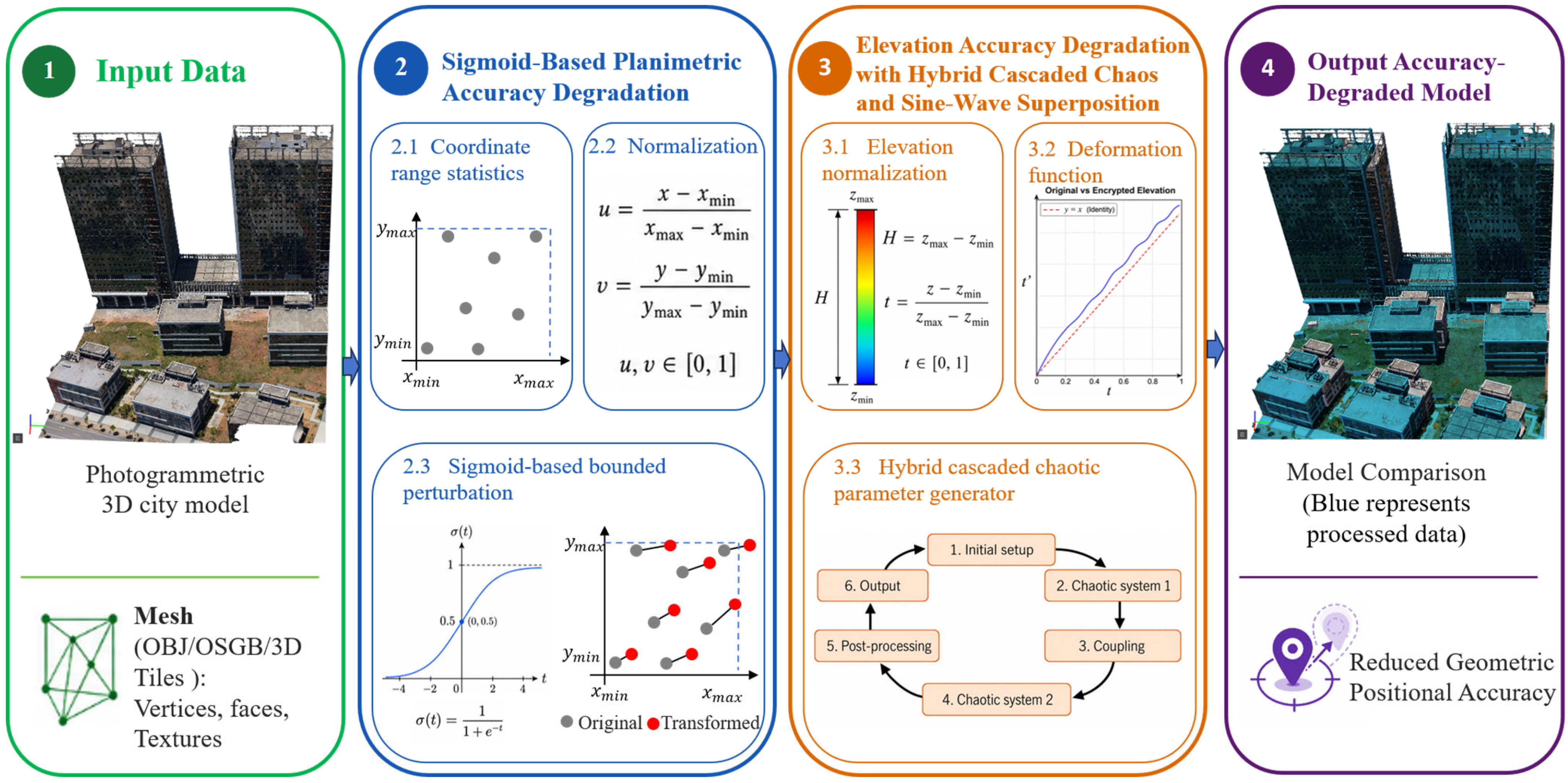
Figure 1. Flowchart of the controlled accuracy-degradation method for photogrammetric 3D city models.
Remotesensing 18 02878 g001
Figure 2. Qualitative interpretation of planimetric accuracy degradation under different target scales (blue represents the processed model): (a) 5 m planimetric displacement, (b) 10 m planimetric displacement, (c) 15 m planimetric displacement.
Remotesensing 18 02878 g002
Figure 3. Displacement vectors of sampled planimetric points under the 10 m target scale. Red points indicate the original positions, blue points indicate the processed positions, and connecting lines represent displacement vectors.
Remotesensing 18 02878 g003
Figure 4. Elevation accuracy-degradation results under different values of k (blue represents the processed model): (a) 5% additional elevation stretching, (b) 10% additional elevation stretching, (c) 15% additional elevation stretching.
Remotesensing 18 02878 g004
Figure 5. Elevation transformation curves and elevation-change profiles (In the upper panels, the red dashed line represents the identity reference z ′ = z ; in the lower panels, it represents the zero-deformation baseline ∆ z = 0 ) for k = 5.0%, 10.0%, and 15.0%: (a) 5% elevation change, (b) 10% elevation change, (c) 15% elevation change.
Remotesensing 18 02878 g005
Figure 6. Detail comparison of the model before and after elevation deformation at k = 5.0%. The red solid line denotes the slant range, while the blue dashed line denotes the building height. (a) Before elevation degradation, (b) after elevation degradation.
Remotesensing 18 02878 g006
Figure 7. Integrated accuracy-degradation results (In the three plots in panel (c), the red dashed lines denote z ′ = z , zero elevation-change, and zero relative-deformation references, respectively) for a low-rise building scene. (a) Model comparison, (b) planimetric displacement, (c) elevation displacement.
Remotesensing 18 02878 g007aRemotesensing 18 02878 g007b
Figure 8. Integrated accuracy-degradation results (In the three plots in panel (c), the red dashed lines denote z ′ = z , zero elevation-change, and zero relative-deformation references, respectively) for a high-rise building scene. (a) Model comparison, (b) planimetric displacement, (c) elevation displacement.
Remotesensing 18 02878 g008
Figure 9. Integrated accuracy-degradation result for an irregular building scene (the original model is rendered in true surface colors, whereas the processed model is shown in blue).
Remotesensing 18 02878 g009
Figure 10. Spatial distribution of the 10 independent checkpoints used for accuracy evaluation.
Remotesensing 18 02878 g010
Table 1. Coordinate displacement and planimetric RMSE under different target deformation scales.
Target Scale (m)Minimum Displacement (m)Maximum Displacement (m)RMSE (m)
54.0006.3254.948
108.00012.6499.895
1512.00018.97414.843
Table 2. Planimetric coordinate displacement of the sampled points.
IDOriginal x (m)Original y (m)Processed x (m)Processed y (m)Δx (m)Δy (m)Distance (m)
193.863220.572102.654221.9968.7901.4248.905
2171.913201.967183.027201.92411.114−0.04311.114
384.069263.64692.572267.4358.5033.7899.309
4120.248219.168129.822220.4879.5741.3199.664
5110.825159.733120.119156.7339.293−3.0009.765
696.612220.234105.484221.6338.8721.3998.981
7111.390149.764120.700146.2979.310−3.4689.935
890.368241.53299.055244.3318.6882.7999.127
972.103164.47780.258161.7358.155−2.7438.604
10108.253221.204117.469222.6759.2171.4719.333
Table 3. Sine-function parameters generated under different chaotic initial values.
x 0 A 1 A 2 f 1 f 2 P 1 P 2
0.12345678000.0941640.1058366.46702.38222.81883.3684
0.12345678100.0962770.1037232.75472.49175.54672.3054
0.12345678200.0823980.1176024.31036.03221.90565.0125
0.12345678300.0914970.1085032.21736.39624.18461.1682
0.12345678400.1248310.0751694.46504.46841.79555.0784
0.12345678500.0722240.1277761.87973.04972.99852.0963
0.12345678600.1467850.0532154.06743.26124.89683.3765
0.12345678700.0620090.1379911.77763.91053.15883.9629
0.12345678800.1488750.0511255.65894.83622.48825.9762
Table 4. Monotonic-violation rates under different nonlinear amplitude bounds, R, (Unit: %).
Initial ValueR = 0.02R = 0.05R = 0.07
0.12345678000.00000.00003.4151
0.12345679000.00000.00005.7853
0.12345680000.00003.600211.325
0.12345681000.00001.11019.6154
0.12345682000.00000.00000.0000
0.12345683000.00001.66519.2504
0.12345684000.00000.00007.2753
0.12345685000.00000.00000.0000
0.12345686000.00000.00000.0000
0.12345687000.00001.395110.1905
Table 5. Height ratios under different chaotic initial values.
Initial ValueHeight Ratio h ′ / h  (%)
0.12345678105.01
0.12345679105.15
0.12345680105.28
0.12345681105.92
0.12345682104.83
0.12345683105.89
0.12345684105.67
0.12345685105.12
0.12345686104.55
0.12345687105.01
Table 6. Direction consistency and spatial-shape coefficient ratio under different chaotic initial values.
x 0 Direction Consistency P (%)Spatial-Shape Coefficient Ratio S (%)
0.1234567800100.0000100.0074
0.1234567900100.0000100.0074
0.1234568000100.0000100.0074
0.123456810099.9932100.0074
0.1234568200100.0000100.0074
0.1234568300100.0000100.0074
0.1234568400100.0000100.0074
0.1234568500100.0000100.0074
0.123456860099.8757100.0074
0.1234568700100.0000100.0074
Table 7. Parameters adopted in the integrated accuracy-degradation experiment.
ParameterValue
Planimetric degradation scale10 m
Sigmoid amplitude setting S x = 2 V x y ;   S y used as auxiliary direction disturbance
Perturbation-threshold settingDirection thresholds used to constrain x- and y-axis offsets
Overall elevation-slope parameter k0.05 (5%)
Maximum nonlinear relative deformation R0.02 (2%)
Number of superimposed sine waves n2
Total sine-wave amplitude Σ A i 0.08
Frequency range[5.0, 6.5]
Phase range[0, 2π]
Logistic control parameter μ 1 4
Cascade control parameter2.3
Binary precision N 1 16
Pre-iteration number N 2 200
Bit extraction position k b 7
Maximum scale-factor amplitude a ≤0.5%
Maximum translation amplitude b ≤0.1% of total elevation range
Table 8. Root-mean-square error of checkpoints (Unit: m).
ModelPlanimetric AccuracyElevation Accuracy3D Accuracy
Original Model0.02500.03840.0458
Processed Model10.23870.090010.2391
Table 9. Object-height measurement accuracy after elevation stretching.
IDGround-Truth Object Height (m)Height After Stretching (m)Relative Object-Height Measurement Error (%)RMSE (%)
110.6611.255.535.24
221.3222.274.45
39.7010.205.15
420.3721.555.79
524.3225.434.56
614.8015.716.15
74.374.615.49
812.7813.364.53
914.8715.735.78
1024.3725.504.61
Table 10. Quantitative evaluation of controlled accuracy degradation for the three datasets.
Evaluation MetricDataset 1Dataset 2Dataset 3
Target relative elevation deformation, ( R z ) (%)5.005.005.00
Actual relative elevation deformation, ( R z ) (%)5.015.305.05
Elevation range (m)186.49131.0941.92
Minimum relative elevation deformation (%)3.383.443.62
Maximum relative elevation deformation (%)6.606.566.40
Mean planimetric displacement, ( R x y ) (m)10.4710.0510.24
Minimum planimetric displacement (m)8.018.008.00
Maximum planimetric displacement (m)12.6312.6512.65
Direction consistency, ( P ) (%)100.00100.00100.00
Spatial-shape coefficient ratio, ( S ) (%)100.0298.6799.71
Number of vertices668,8901,183,795130,353,583
Number of faces1,329,5982,348,881205,555,992
Coverage area (km2)0.660.0462.93
Processing time (s)42.7769.769109.21
Table 11. Ablation study of the proposed method.
Ablation SettingXY RMSE (m)Min-Max XY Displacement (m)Direction Consistency (%)Mean Angle Deviation (deg)Spatial-Shape Coefficient Ratio (%)Processing Time (s)
Full method10.478.01–12.63100.001.00100.0242.21
Without Sigmoid10.0010.00–10.00100.001.09100.0043.44
Without sine-wave superposition10.478.01–12.63100.000.62100.0244.89
Without chaotic parameter generation10.478.01–12.63100.000.89100.0248.39
Without post-processing adjustment10.478.01–12.63100.000.99100.0252.48
Table 12. Accuracy of known-point recovery attacks using four corner control points.
Recovery ModelXY RMSE (m)Z RMSE (m)3D RMSE (m)
Translation2.160.072.17
Affine0.280.050.29
Quadratic polynomial0.490.050.49
Disclaimer/Publisher’s Note: The statements, opinions and data contained in all publications are solely those of the individual author(s) and contributor(s) and not of MDPI and/or the editor(s). MDPI and/or the editor(s) disclaim responsibility for any injury to people or property resulting from any ideas, methods, instructions or products referred to in the content.