Author Contributions
Conceptualization, Y.C. and C.L.; methodology, Y.C.; software, Y.C.; validation, Y.C., Z.W., J.J., C.H., Y.S. and S.Z.; formal analysis, Y.C.; investigation, Y.C.; resources, C.L.; data curation, Y.C.; writing–original draft preparation, Y.C.; writing–review and editing, Y.C. and C.L.; visualization, Y.C.; supervision, C.L.; project administration, C.L.; funding acquisition, C.L. All authors have read and agreed to the published version of the manuscript.
Figure 1.
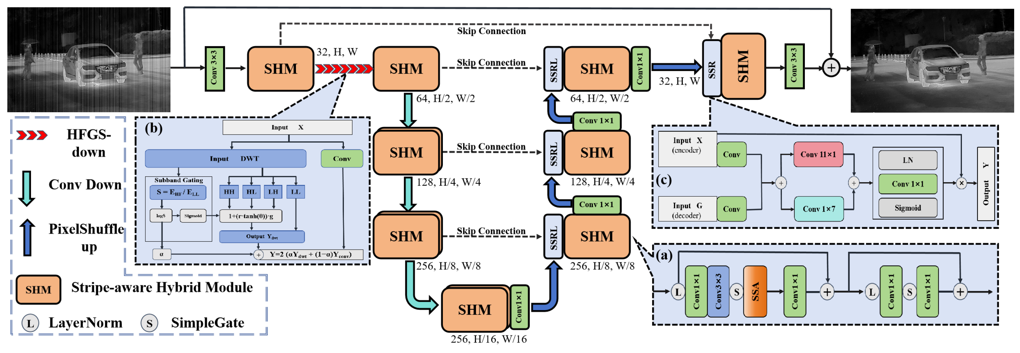
Overall architecture of the proposed SFPRNet for infrared image destriping. (a) Stripe-Aware Hybrid Module. (b) High-Frequency Gated Sub-band Downsampling module. (c) Structure-Guided Skip Refinement module.
Figure 1.
Overall architecture of the proposed SFPRNet for infrared image destriping. (a) Stripe-Aware Hybrid Module. (b) High-Frequency Gated Sub-band Downsampling module. (c) Structure-Guided Skip Refinement module.
Figure 2.
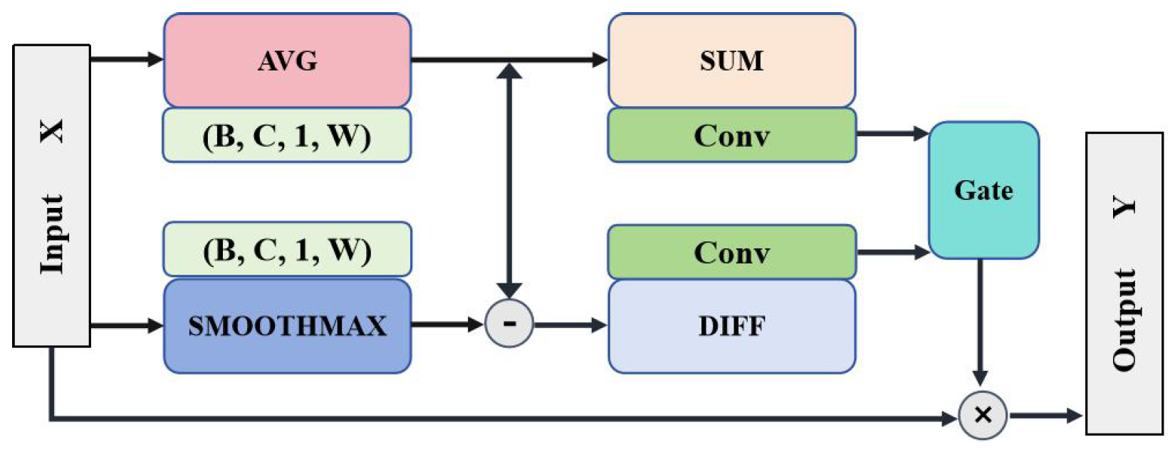
Architecture of the Stripe-Aware Spatial Attention (SSA) module.
Figure 2.
Architecture of the Stripe-Aware Spatial Attention (SSA) module.
Figure 3.
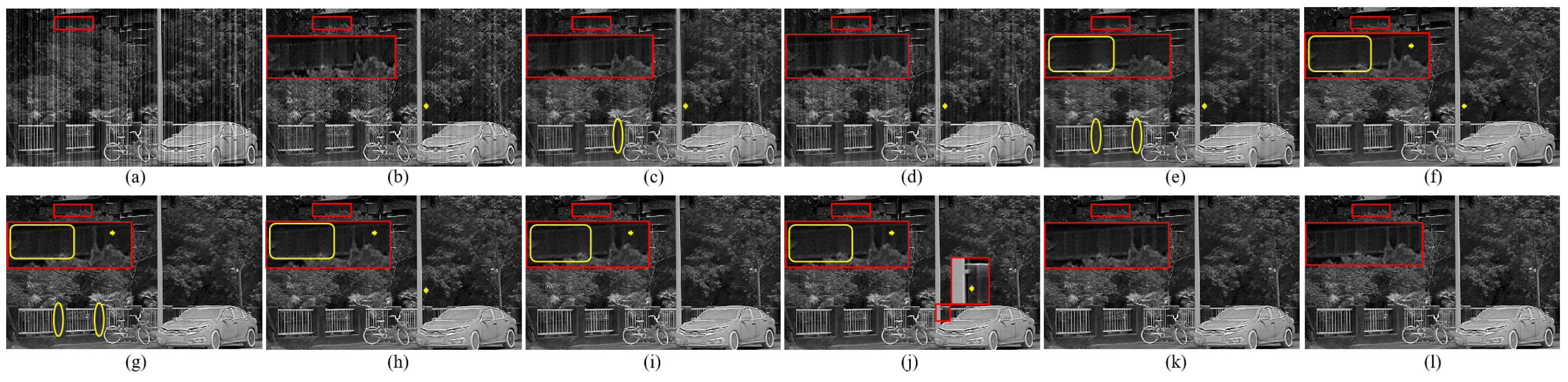
Destriping results of different methods on infrared images corrupted by simulated Gaussian stripe noise. Stripe residuals and blurred image details are marked by yellow arrows and boxes, respectively. (a) Degraded. (b) ADOM. (c) GF. (d) MIRE. (e) SNRCNN. (f) DLS-NUC. (g) SNRWDNN. (h) NAFNet. (i) DSCGAN. (j) ASCNet. (k) Ours. (l) GT.
Figure 3.
Destriping results of different methods on infrared images corrupted by simulated Gaussian stripe noise. Stripe residuals and blurred image details are marked by yellow arrows and boxes, respectively. (a) Degraded. (b) ADOM. (c) GF. (d) MIRE. (e) SNRCNN. (f) DLS-NUC. (g) SNRWDNN. (h) NAFNet. (i) DSCGAN. (j) ASCNet. (k) Ours. (l) GT.
Figure 4.
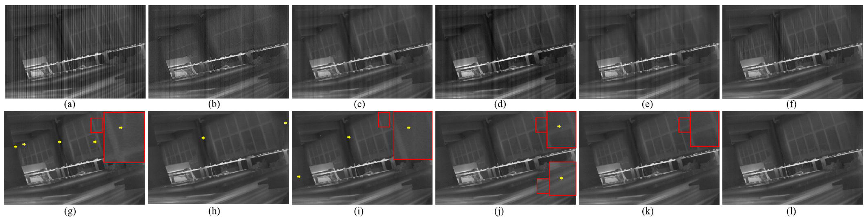
Destriping results of different methods on infrared images corrupted by simulated wide-period stripe noise. Stripe residuals and blurred image details are marked by yellow arrows and red boxes, respectively. (a) Degraded. (b) ADOM. (c) GF. (d) MIRE. (e) SNRCNN. (f) DLS-NUC. (g) SNRWDNN. (h) NAFNet. (i) DSCGAN. (j) ASCNet. (k) Ours. (l) GT.
Figure 4.
Destriping results of different methods on infrared images corrupted by simulated wide-period stripe noise. Stripe residuals and blurred image details are marked by yellow arrows and red boxes, respectively. (a) Degraded. (b) ADOM. (c) GF. (d) MIRE. (e) SNRCNN. (f) DLS-NUC. (g) SNRWDNN. (h) NAFNet. (i) DSCGAN. (j) ASCNet. (k) Ours. (l) GT.
Figure 5.
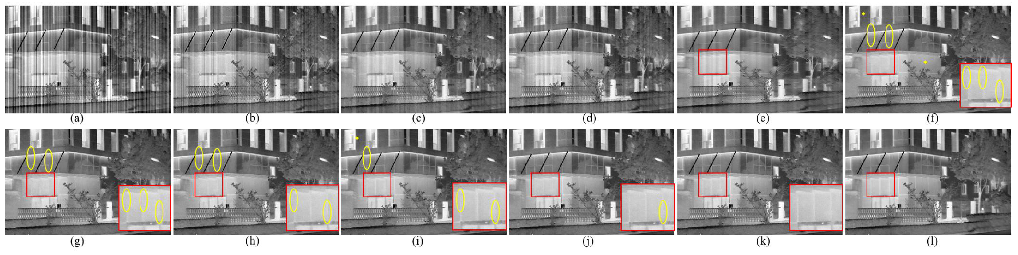
Destriping results of different methods on infrared images corrupted by simulated mixed Gaussian noise. Stripe residuals and blurred image details are marked by yellow arrows and boxes, respectively. (a) Degraded. (b) ADOM. (c) GF. (d) MIRE. (e) SNRCNN. (f) DLS-NUC. (g) SNRWDNN. (h) NAFNet. (i) DSCGAN. (j) ASCNet. (k) Ours. (l) GT.
Figure 5.
Destriping results of different methods on infrared images corrupted by simulated mixed Gaussian noise. Stripe residuals and blurred image details are marked by yellow arrows and boxes, respectively. (a) Degraded. (b) ADOM. (c) GF. (d) MIRE. (e) SNRCNN. (f) DLS-NUC. (g) SNRWDNN. (h) NAFNet. (i) DSCGAN. (j) ASCNet. (k) Ours. (l) GT.
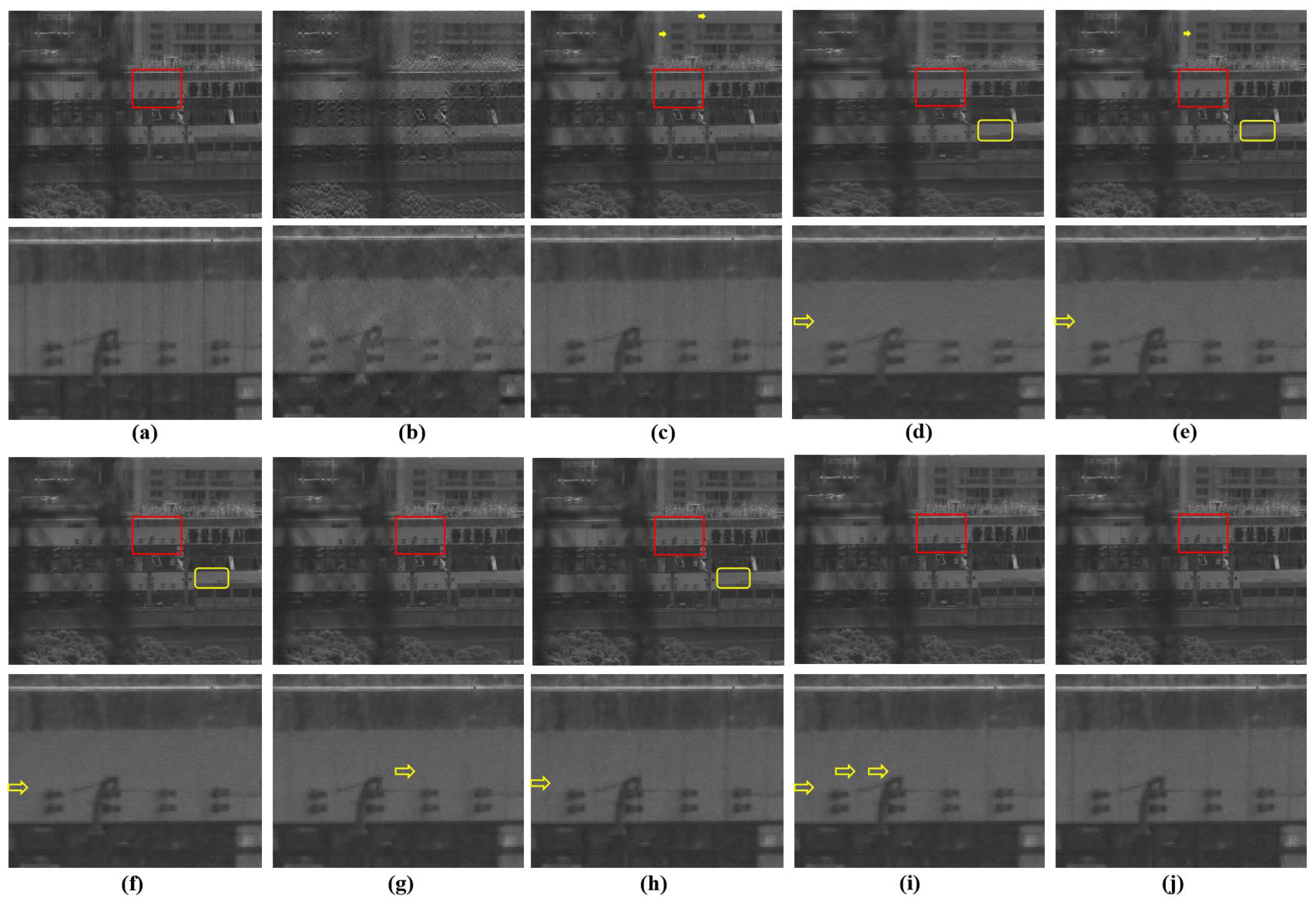
Figure 6.
Destriping results of different methods on real infrared images. Stripe residuals and blurred image details are marked by yellow arrows and boxes, respectively. (a) Degraded. (b) ADOM. (c) GF. (d) SNRCNN. (e) DLS-NUC. (f) SNRWDNN. (g) NAFNet. (h) DSCGAN. (i) ASCNet. (j) Ours.
Figure 6.
Destriping results of different methods on real infrared images. Stripe residuals and blurred image details are marked by yellow arrows and boxes, respectively. (a) Degraded. (b) ADOM. (c) GF. (d) SNRCNN. (e) DLS-NUC. (f) SNRWDNN. (g) NAFNet. (h) DSCGAN. (i) ASCNet. (j) Ours.
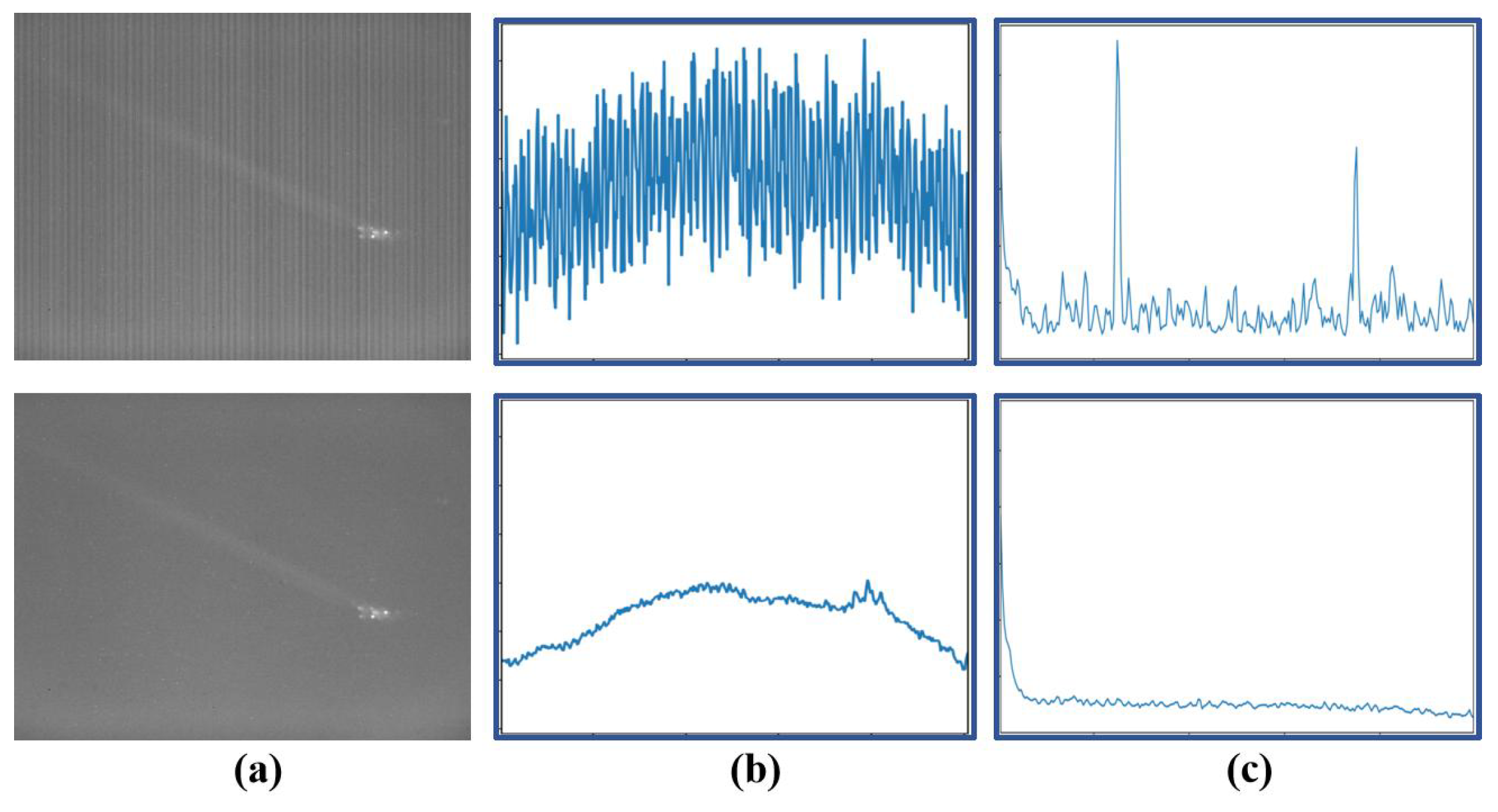
Figure 7.
Spatial- and frequency-domain analysis on self-acquired real infrared remote-sensing data. (a) Images before (top) and after (bottom) destriping. (b) Corresponding column-wise mean profiles. (c) Corresponding horizontal frequency spectra.
Figure 7.
Spatial- and frequency-domain analysis on self-acquired real infrared remote-sensing data. (a) Images before (top) and after (bottom) destriping. (b) Corresponding column-wise mean profiles. (c) Corresponding horizontal frequency spectra.
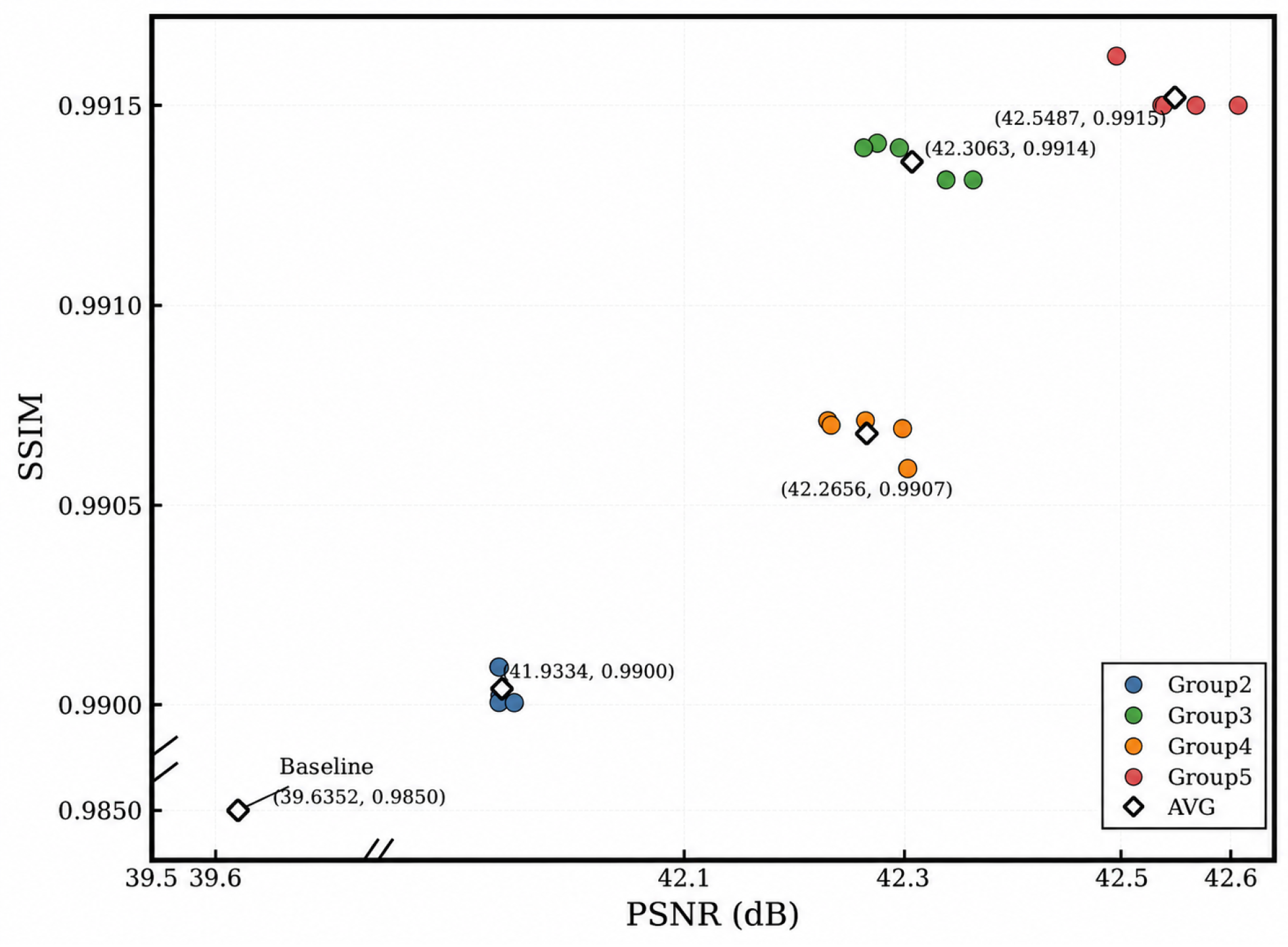
Figure 8.
Multi-seed robustness analysis of SFPRNet in the PSNR–SSIM space.
Figure 8.
Multi-seed robustness analysis of SFPRNet in the PSNR–SSIM space.
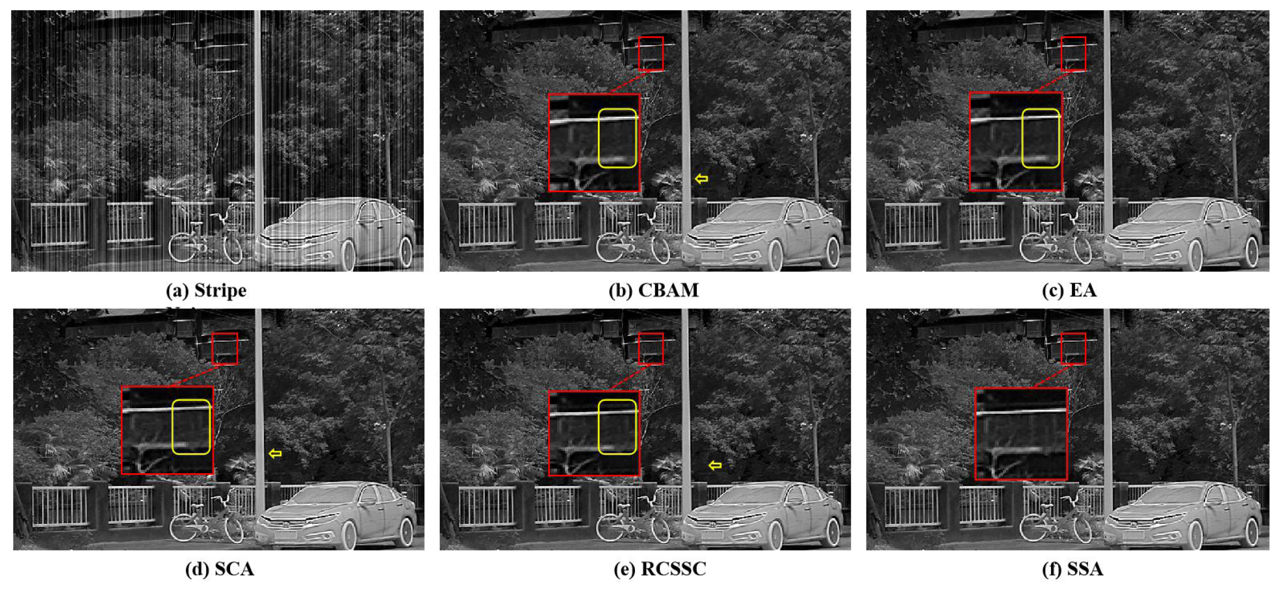
Figure 9.
Destriping results of different attention mechanisms on infrared images corrupted by simulated Gaussian stripe noise. Stripe residuals and blurred details are marked by arrows and boxes, respectively.
Figure 9.
Destriping results of different attention mechanisms on infrared images corrupted by simulated Gaussian stripe noise. Stripe residuals and blurred details are marked by arrows and boxes, respectively.
Figure 10.
Visualization of the feature responses of different SSA branches. (a) Degraded. (b) AVG. (c) SMOOTHMAX. (d) DIFF.
Figure 10.
Visualization of the feature responses of different SSA branches. (a) Degraded. (b) AVG. (c) SMOOTHMAX. (d) DIFF.
Figure 11.
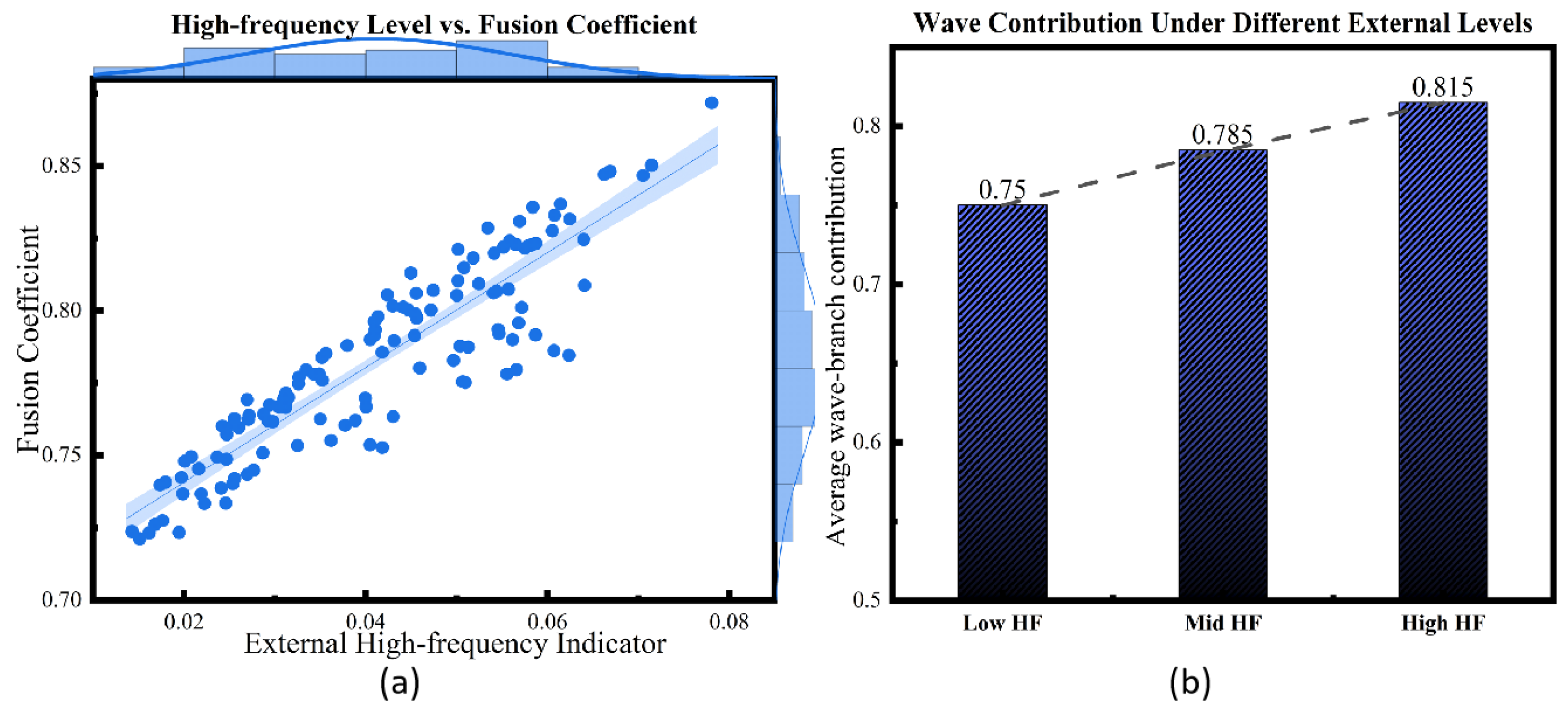
Visualization of HFGS-Down: (a) relationship between high-frequency level and fusion coefficient; (b) wavelet-branch contribution under different high-frequency groups.
Figure 11.
Visualization of HFGS-Down: (a) relationship between high-frequency level and fusion coefficient; (b) wavelet-branch contribution under different high-frequency groups.
Figure 12.
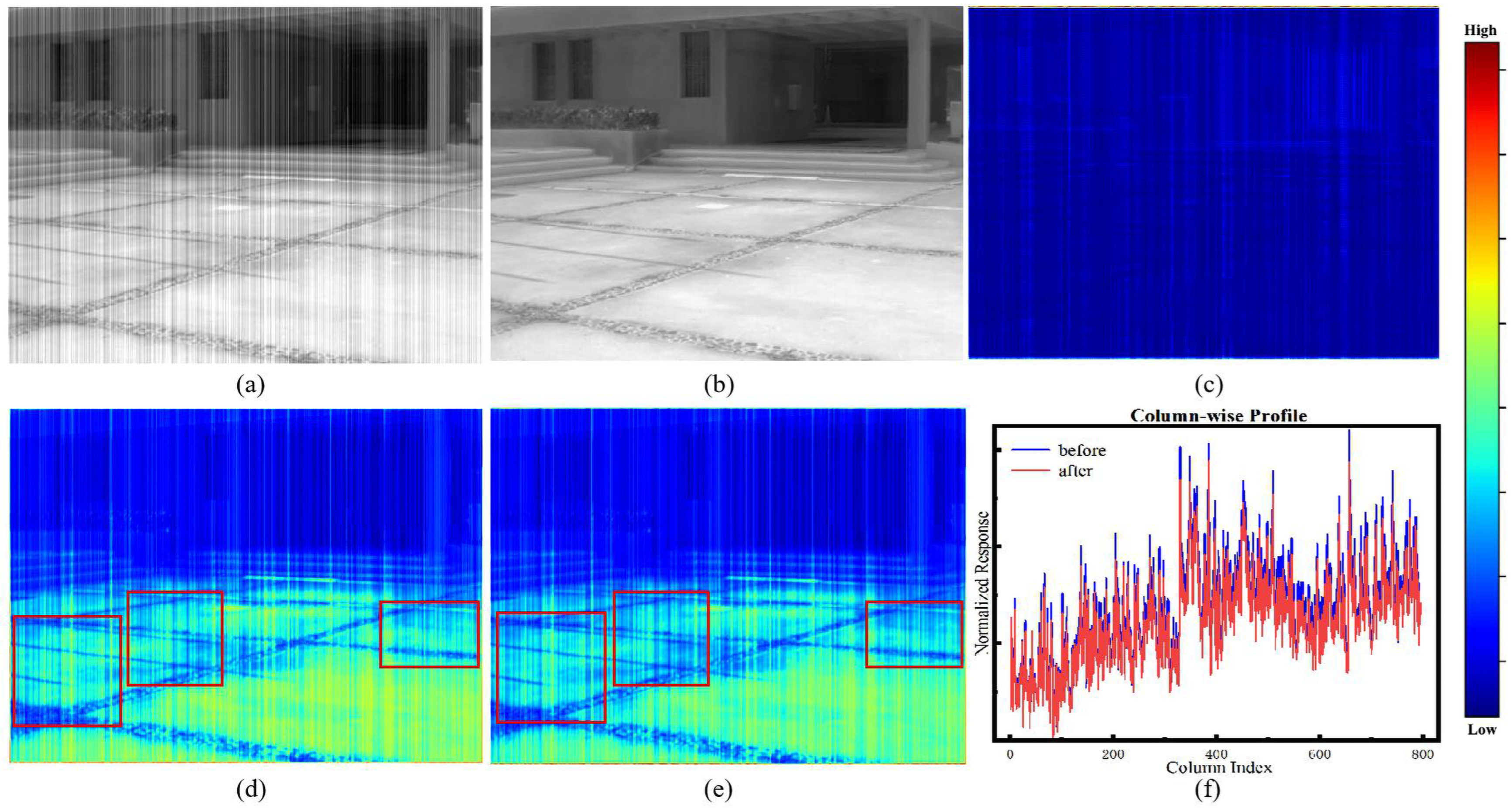
Visual analysis of the SSR ablation. (a) Input image corrupted by stripe noise. (b) Restored output after destriping. (c) Learned gating mask of SSR. (d) Shallow feature response before gating. (e) Shallow feature response after gating. (f) Column-wise statistical response curve. Red boxes in (d,e) highlight representative regions for visual comparison of shallow feature responses before and after gating.
Figure 12.
Visual analysis of the SSR ablation. (a) Input image corrupted by stripe noise. (b) Restored output after destriping. (c) Learned gating mask of SSR. (d) Shallow feature response before gating. (e) Shallow feature response after gating. (f) Column-wise statistical response curve. Red boxes in (d,e) highlight representative regions for visual comparison of shallow feature responses before and after gating.
Figure 13.
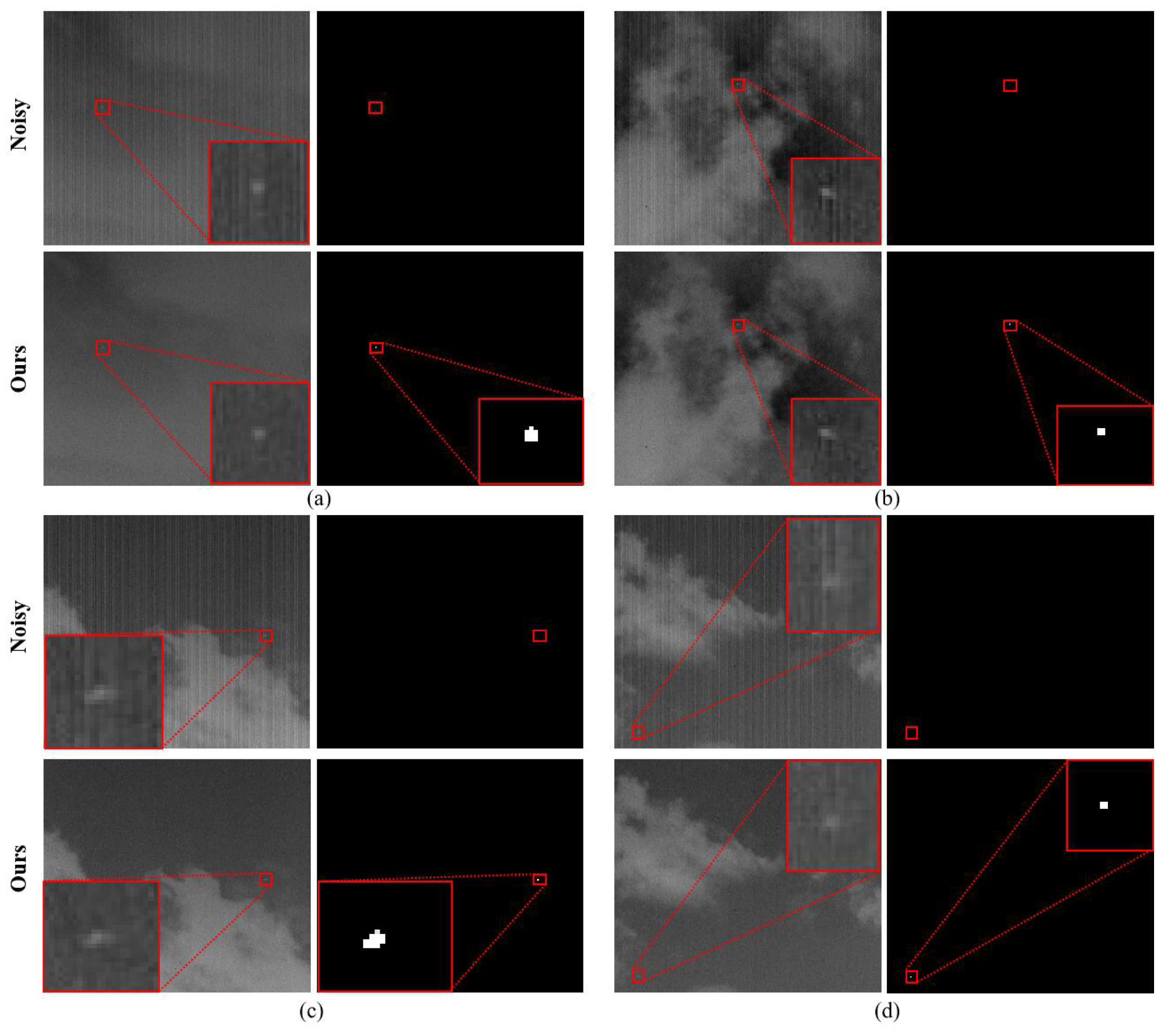
IRSTD results before and after destriping on a real noisy small-target dataset. (a–d) Four representative examples.
Figure 13.
IRSTD results before and after destriping on a real noisy small-target dataset. (a–d) Four representative examples.
Table 1.
Quantitative comparison of different methods on the test sets in terms of PSNR and SSIM.
Table 1.
Quantitative comparison of different methods on the test sets in terms of PSNR and SSIM.
| Category | Index | ADOM | GF | MIRE | SNRCNN | DLS-NUC | SNRWDNN | NAFNet | DSCGAN | ASCNet | Ours |
|---|
| IR700-100 |
| Gaussian | PSNR↑ | 30.0083 | 34.8742 | 32.8174 | 33.7442 | 38.1721 | 38.0898 | 39.6361 | 41.3426 | 42.1435 | 42.6997 |
| SSIM↑ | 0.8547 | 0.9488 | 0.9373 | 0.9348 | 0.9778 | 0.9773 | 0.9848 | 0.9892 | 0.9902 | 0.9920 |
| Wide | PSNR↑ | 30.6482 | 35.8570 | 33.7246 | 34.2055 | 37.9809 | 38.4726 | 40.2509 | 41.7473 | 42.0397 | 42.8232 |
| SSIM↑ | 0.8766 | 0.9604 | 0.9527 | 0.9399 | 0.9708 | 0.9770 | 0.9856 | 0.9891 | 0.9887 | 0.9919 |
| Mixed | PSNR↑ | 26.9224 | 30.1896 | 29.3211 | 30.2246 | 31.9537 | 31.9174 | 32.6617 | 33.2814 | 33.2906 | 33.5054 |
| SSIM↑ | 0.6183 | 0.7401 | 0.7199 | 0.7576 | 0.7689 | 0.7706 | 0.7819 | 0.7840 | 0.7788 | 0.7843 |
| ESPOL-10 |
| Gaussian | PSNR↑ | 31.7440 | 34.8661 | 33.2875 | 34.6076 | 38.5380 | 38.2140 | 39.7665 | 40.9548 | 42.0727 | 42.0505 |
| SSIM↑ | 0.8482 | 0.9391 | 0.9213 | 0.9271 | 0.9728 | 0.9682 | 0.9802 | 0.9815 | 0.9868 | 0.9869 |
| Wide | PSNR↑ | 33.7932 | 39.3867 | 36.4989 | 37.7068 | 40.7759 | 40.5679 | 42.2772 | 42.8157 | 43.2341 | 43.7391 |
| SSIM↑ | 0.9010 | 0.9758 | 0.9649 | 0.9551 | 0.9773 | 0.9747 | 0.9848 | 0.9860 | 0.9878 | 0.9905 |
| Mixed | PSNR↑ | 29.3728 | 32.1810 | 31.1669 | 32.4177 | 34.3047 | 34.2190 | 35.1212 | 35.8523 | 35.7840 | 35.8576 |
| SSIM↑ | 0.6807 | 0.7958 | 0.7750 | 0.8074 | 0.8302 | 0.8287 | 0.8455 | 0.8484 | 0.8402 | 0.8416 |
| DLS-NUC-7 |
| Gaussian | PSNR↑ | 32.5929 | 36.7779 | 27.8496 | 36.0688 | 39.7410 | 39.8097 | 41.1839 | 42.2749 | 42.5898 | 43.1999 |
| SSIM↑ | 0.8658 | 0.9574 | 0.9119 | 0.9434 | 0.9814 | 0.9786 | 0.9849 | 0.9893 | 0.9891 | 0.9900 |
| Wide | PSNR↑ | 33.3475 | 39.3535 | 30.6004 | 37.5067 | 39.7598 | 40.6534 | 42.8129 | 43.2991 | 43.3380 | 43.7635 |
| SSIM↑ | 0.8945 | 0.9753 | 0.9377 | 0.9542 | 0.9700 | 0.9781 | 0.9886 | 0.9895 | 0.9899 | 0.9907 |
| Mixed | PSNR↑ | 28.6296 | 32.0168 | 26.9560 | 32.2658 | 33.4090 | 33.5140 | 33.9538 | 34.1541 | 34.1894 | 34.3356 |
| SSIM↑ | 0.5839 | 0.7006 | 0.6539 | 0.7245 | 0.7251 | 0.7250 | 0.7331 | 0.7333 | 0.7280 | 0.7333 |
| ICSRN-6 |
| Gaussian | PSNR↑ | 28.8455 | 36.1407 | 20.3065 | 32.9996 | 37.3004 | 37.4397 | 37.9297 | 38.5954 | 38.3843 | 38.6429 |
| SSIM↑ | 0.8565 | 0.9724 | 0.8361 | 0.9391 | 0.9836 | 0.9850 | 0.9900 | 0.9935 | 0.9743 | 0.9946 |
| Wide | PSNR↑ | 28.0229 | 33.8100 | 21.6958 | 30.6477 | 33.8766 | 34.8384 | 35.6340 | 37.6272 | 35.7142 | 38.0046 |
| SSIM↑ | 0.8376 | 0.9625 | 0.6896 | 0.9016 | 0.9598 | 0.9747 | 0.9846 | 0.9905 | 0.9597 | 0.9919 |
| Mixed | PSNR↑ | 26.4836 | 29.8587 | 19.2597 | 29.2005 | 30.8913 | 30.9439 | 31.3420 | 31.1852 | 31.0959 | 31.2243 |
| SSIM↑ | 0.6760 | 0.7898 | 0.8306 | 0.7825 | 0.8059 | 0.8093 | 0.8173 | 0.8104 | 0.8027 | 0.8195 |
| FLIR-5 |
| Gaussian | PSNR↑ | 31.3692 | 36.0267 | 29.0257 | 34.7769 | 38.2809 | 38.3639 | 39.2340 | 40.2687 | 41.0845 | 41.1531 |
| SSIM↑ | 0.8784 | 0.9626 | 0.9440 | 0.9508 | 0.9849 | 0.9854 | 0.9900 | 0.9926 | 0.9941 | 0.9949 |
| Wide | PSNR↑ | 31.7260 | 36.9682 | 28.6674 | 35.6216 | 39.1034 | 39.1463 | 40.0750 | 41.0609 | 41.0922 | 41.3658 |
| SSIM↑ | 0.8808 | 0.9627 | 0.9434 | 0.9544 | 0.9838 | 0.9849 | 0.9893 | 0.9915 | 0.9909 | 0.9937 |
| Mixed | PSNR↑ | 28.7537 | 31.0877 | 28.0160 | 31.2624 | 32.6887 | 32.6225 | 33.1430 | 33.3958 | 33.4278 | 33.6637 |
| SSIM↑ | 0.6705 | 0.7643 | 0.7488 | 0.7815 | 0.7916 | 0.7931 | 0.8033 | 0.8043 | 0.7969 | 0.8045 |
Table 2.
No-reference quantitative comparison on real infrared images.
Table 2.
No-reference quantitative comparison on real infrared images.
| Metric
| ADOM | GF | SNRCNN | DLS-NUC | SNRWDNN | NAFNet | DSCGAN | ASCNet | Ours |
|---|
| ↓ | 0.1029 | 0.0817 | 0.0726 | 0.0787 | 0.0785 | 0.0784 | 0.0815 | 0.0792 | 0.0776 |
| NIQE↓ | 8.7811 | 5.1341 | 6.5920 | 5.9685 | 5.7795 | 5.1743 | 5.1067 | 5.2968 | 4.9063 |
Table 3.
Step-wise system-level ablation of the proposed mismatch rectification chain.
Table 3.
Step-wise system-level ablation of the proposed mismatch rectification chain.
| Group | Baseline | SSA | HFGS-Down | SSR | PSNR↑/SSIM↑ |
|---|
| 1 | ✓ | ✕ | ✕ | ✕ | 39.6352/0.9850 |
| 2 | ✓ | ✓ | ✕ | ✕ | 41.9334/0.9900 |
| 3 | ✓ | ✓ | ✓ | ✕ | 42.3063/0.9914 |
| 4 | ✓ | ✓ | ✕ | ✓ | 42.2656/0.9907 |
| 5 | ✓ | ✓ | ✓ | ✓ | 42.5487/0.9915 |
Table 4.
Quantitative comparison of different attention modules.
Table 4.
Quantitative comparison of different attention modules.
| Method | PSNR↑ | SSIM↑ | Params (M)↓ | FLOPs (G)↓ |
|---|
| CBAM | 39.7568 | 0.9857 | 3.303 | 10.779 |
| EA | 39.9951 | 0.9864 | 4.807 | 16.364 |
| SCA | 39.6352 | 0.9850 | 3.640 | 10.745 |
| RCSSC | 41.3384 | 0.9881 | 4.119 | 18.168 |
| SSA | 41.9344 | 0.9900 | 3.644 | 10.797 |
Table 5.
Ablation study of the internal statistical branches in SSA.
Table 5.
Ablation study of the internal statistical branches in SSA.
| U-Net | AVG | SMOOTHMAX | DIFF | PSNR↑/SSIM↑ |
|---|
| ✓ | ✕ | ✕ | ✕ | 39.6352/0.9850 |
| ✓ | ✓ | ✕ | ✕ | 41.7543/0.9897 |
| ✓ | ✓ | ✓ | ✕ | 41.8895/0.9900 |
| ✓ | ✓ | ✓ | ✓ | 41.9344/0.9900 |
Table 6.
Quantitative comparison of different wavelet bases in HFGS-Down.
Table 6.
Quantitative comparison of different wavelet bases in HFGS-Down.
| Wavelet Basis | Haar | db2 | sym5 | coif1 |
|---|
| PSNR↑ | 42.2676 | 42.0434 | 42.0675 | 42.1090 |
| SSIM↑ | 0.9914 | 0.9911 | 0.9910 | 0.9910 |
Table 7.
Quantitative comparison of different downsampling strategies.
Table 7.
Quantitative comparison of different downsampling strategies.
| Method | Conv-Only | DWT-Only | Conv + DWT | HFGS-Down |
|---|
| PSNR↑ | 41.9344 | 42.1165 | 42.1524 | 42.2784 |
| SSIM↑ | 0.9900 | 0.9910 | 0.9911 | 0.9914 |
Table 8.
Ablation on sub-band gating strategies of HFGS-Down.
Table 8.
Ablation on sub-band gating strategies of HFGS-Down.
| Method | PSNR↑ | SSIM↑ |
|---|
| HL/LL | 42.1183 | 0.9913 |
| (HL + LH + HH)/LL | 42.2784 | 0.9914 |
Table 9.
Quantitative comparison of different skip gating strategies.
Table 9.
Quantitative comparison of different skip gating strategies.
| Method | PSNR↑ | SSIM↑ | Params (M)↓ |
|---|
| Baseline | 41.9344 | 0.9900 | 3.644 |
| SSR-Lite | 42.1798 | 0.9903 | 3.802 |
| SSR | 42.2516 | 0.9904 | 3.808 |
| SSR + SSR-Lite | 42.2331 | 0.9907 | 3.803 |
Table 10.
Computational efficiency and scalability of SFPRNet at different input resolutions.
Table 10.
Computational efficiency and scalability of SFPRNet at different input resolutions.
| Input Resolution | Avg. Inference Time (ms) | Peak GPU Memory (MB) | FPS |
|---|
| 18.6596 | 191.25 | 53.5917 |
| 25.6298 | 381.00 | 39.0171 |
| 30.9626 | 444.25 | 32.2970 |
| 94.7764 | 1140.00 | 10.5512 |
Table 11.
Quantitative comparison of downstream infrared small-target detection performance with different destriping preprocessing methods.
Table 11.
Quantitative comparison of downstream infrared small-target detection performance with different destriping preprocessing methods.
| Method | UIU-Net | RDIAN | DNA-Net |
|---|
| F-Measure↑ | F-Measure↑ | F-Measure↑ |
|---|
| Noisy | 72.6010/0.5078/50.3540/66.9806 | 73.0380/0.0687/34.4587/51.2554 | 88.1980/1.1597/60.4434/75.3455 |
| MIRE | 74.7475/0.4883/50.2041/66.8478 | 70.5063/0.0534/40.0875/57.2321 | 89.9746/2.1973/58.0863/73.4868 |
| ASCNet | 82.9949/0.5469/52.6240/68.9590 | 76.9036/0.0687/38.3286/55.4167 | 92.8934/2.2888/60.6533/75.5083 |
| SFPRNet | 85.3535/0.5469/52.8501/69.1529 | 79.4768/0.0687/38.3701/55.4601 | 94.6701/2.1973/60.6827/75.5311 |





 ,
,