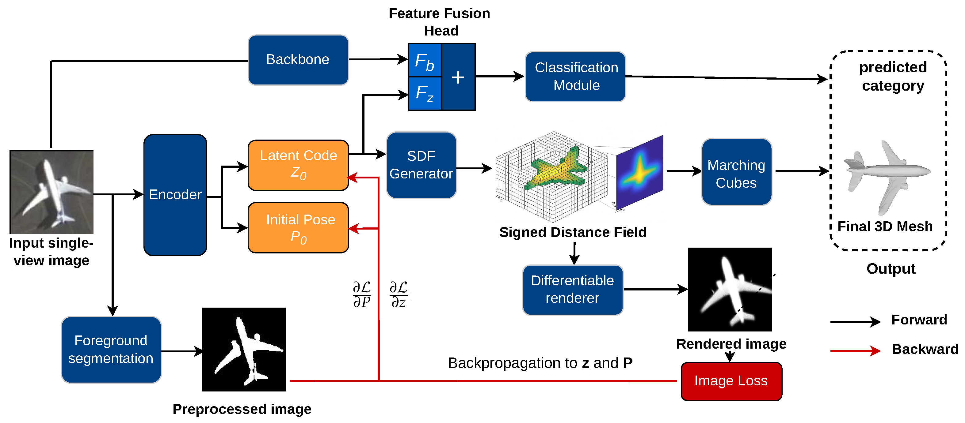
Figure 1.
The overall architecture of our method.
Figure 1.
The overall architecture of our method.
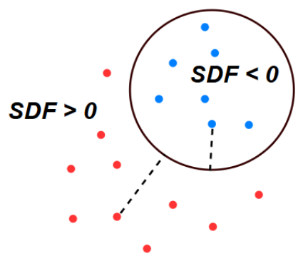
Figure 2.
The definition of Signed Distance Field.
Figure 2.
The definition of Signed Distance Field.
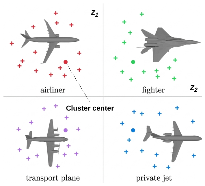
Figure 3.
Four categories of aircraft in our cluster-aware prior learning: airliner, transport, fighter, and private plane.
Figure 3.
Four categories of aircraft in our cluster-aware prior learning: airliner, transport, fighter, and private plane.
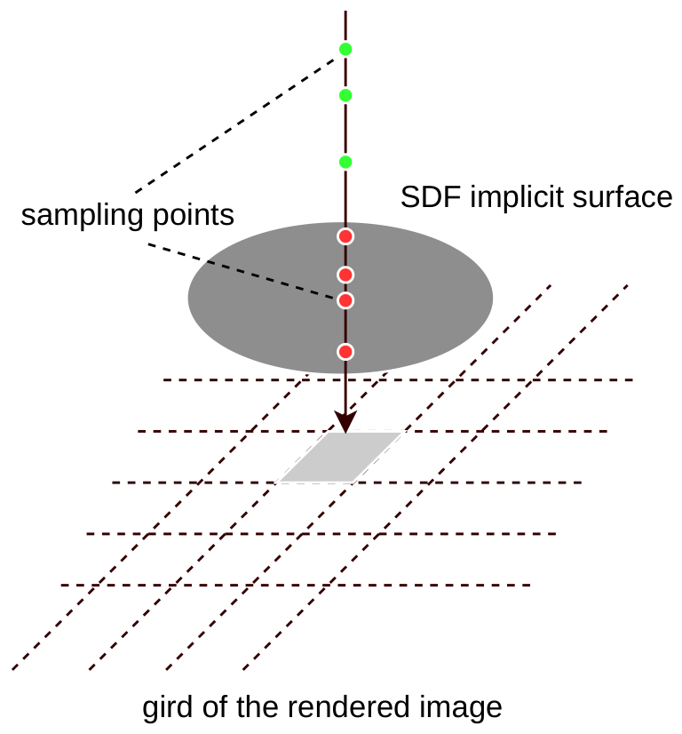
Figure 4.
The differentiable volume rendering framework.
Figure 4.
The differentiable volume rendering framework.
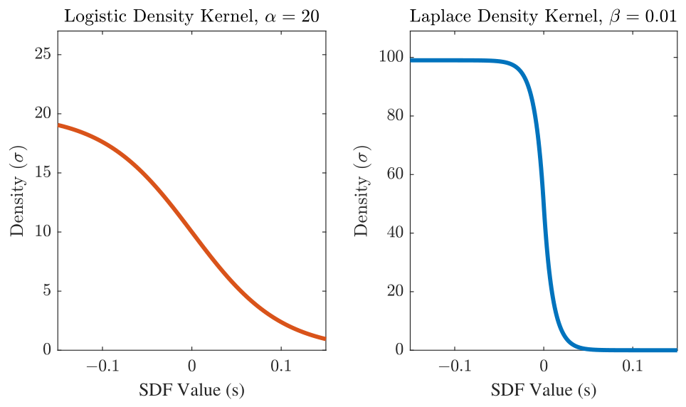
Figure 5.
Two rendering kernels designed for volume rendering.
Figure 5.
Two rendering kernels designed for volume rendering.
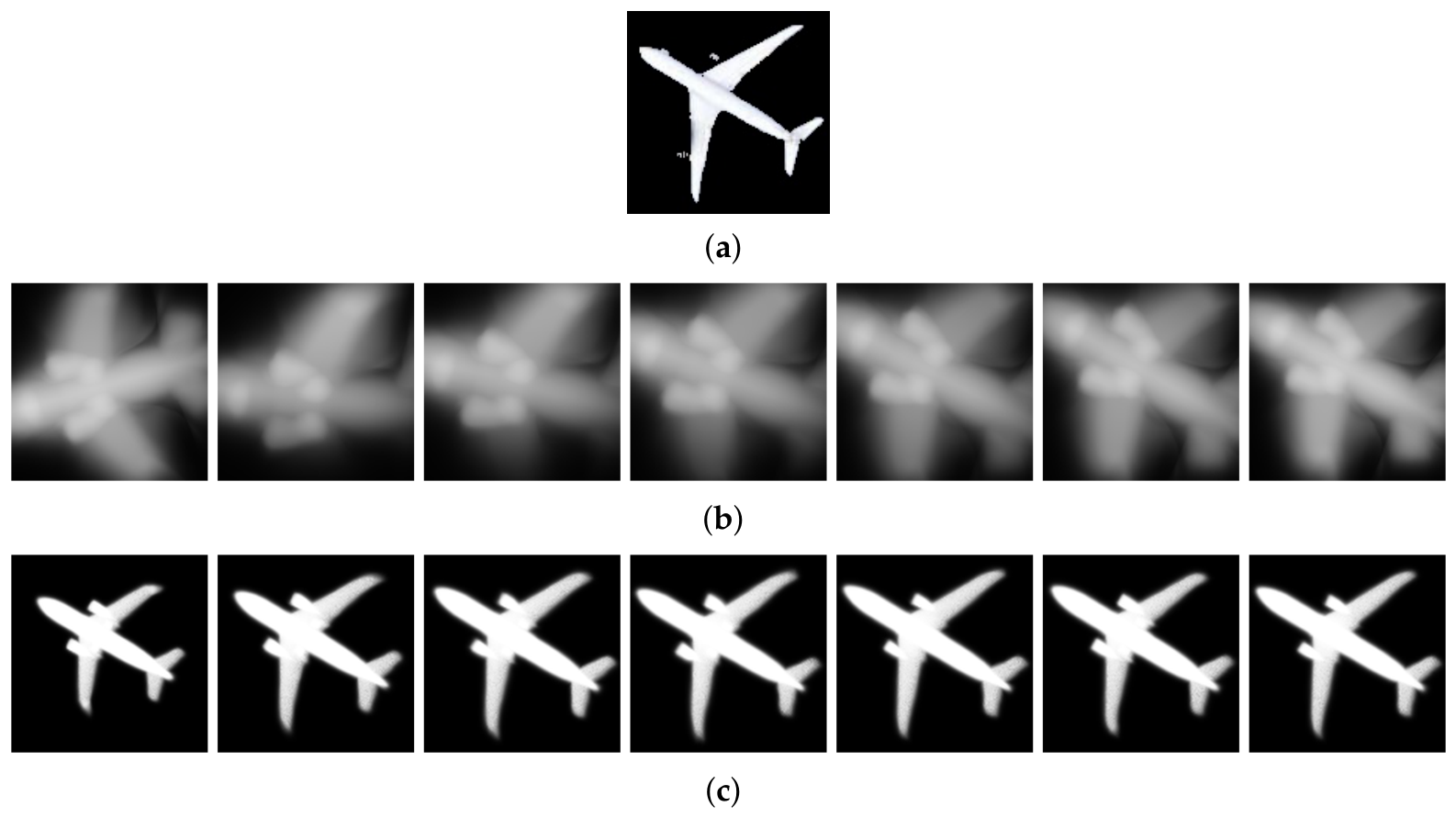
Figure 6.
Example of the two-stage optimization process. (a) the preprocessed remote sensing images; (b) the first-stage optimization process image sequence using the logistic kernel; (c) the second-stage optimization process of the image sequence using the Laplace kernel.
Figure 6.
Example of the two-stage optimization process. (a) the preprocessed remote sensing images; (b) the first-stage optimization process image sequence using the logistic kernel; (c) the second-stage optimization process of the image sequence using the Laplace kernel.
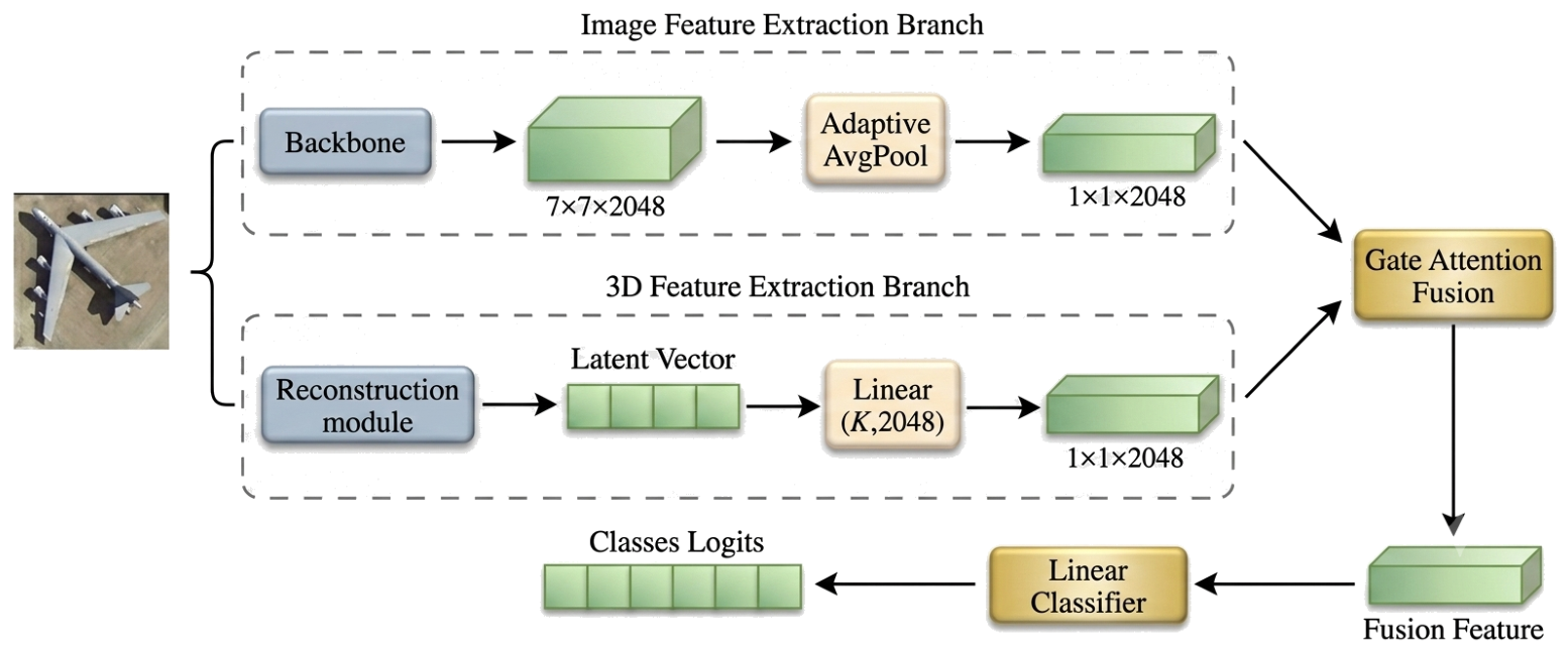
Figure 7.
The classification framework with gated attention fusion mechanism.
Figure 7.
The classification framework with gated attention fusion mechanism.
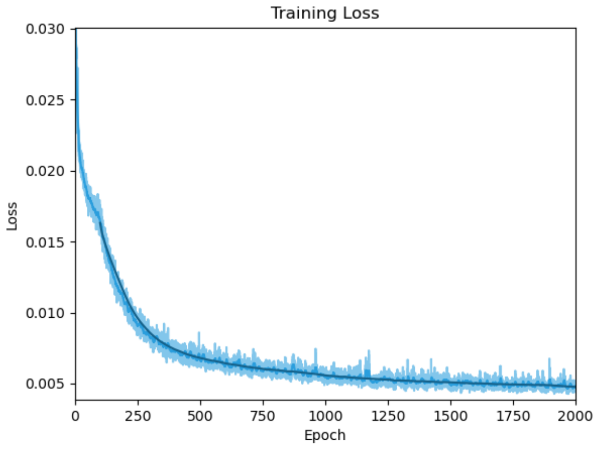
Figure 8.
The change in loss during the training process of the SDF generation network.
Figure 8.
The change in loss during the training process of the SDF generation network.
Figure 9.
The transition process from passenger aircraft to fighter aircraft in the latent space.
Figure 9.
The transition process from passenger aircraft to fighter aircraft in the latent space.
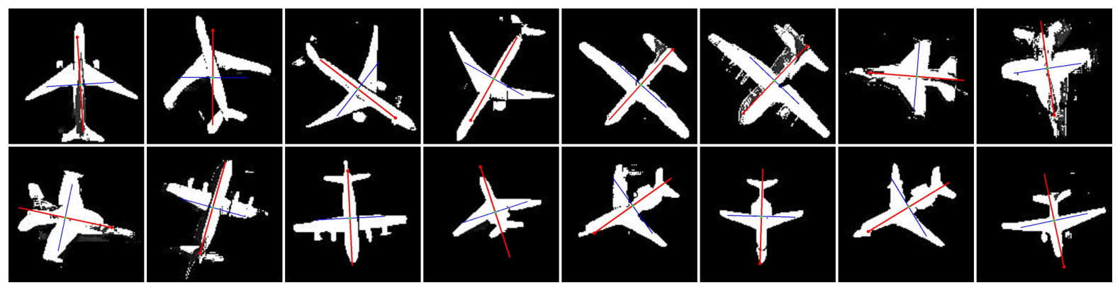
Figure 10.
Test of the pose estimation module, where the red lines represent the first principal component direction and the blue lines indicate its orthogonal direction.
Figure 10.
Test of the pose estimation module, where the red lines represent the first principal component direction and the blue lines indicate its orthogonal direction.
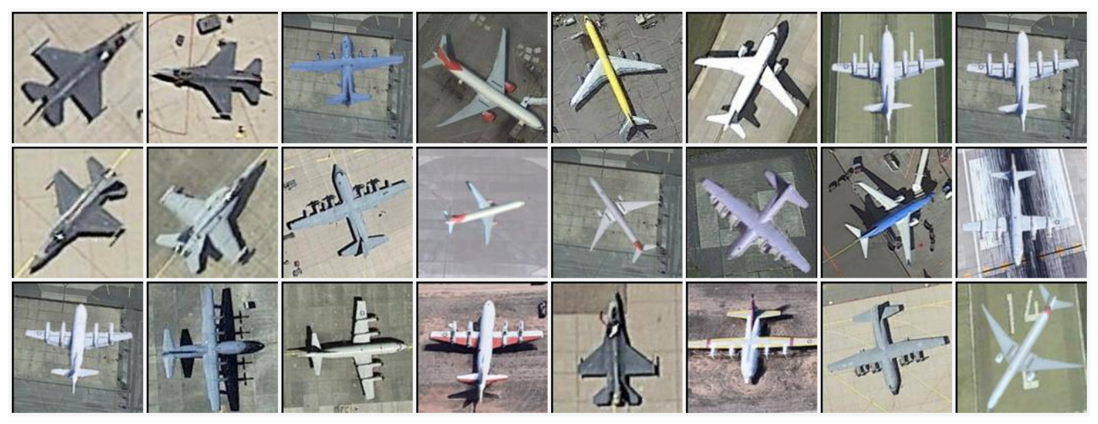
Figure 11.
Some images from the remote sensing image dataset.
Figure 11.
Some images from the remote sensing image dataset.
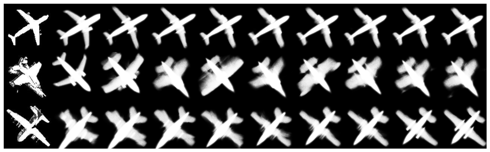
Figure 12.
Rendered image sequence of the latent vector optimization process. The first item in each row is the segmented target image. The nine items on the right correspond to the training progress at 0, 250, 500, …, and 2000 epochs, respectively.
Figure 12.
Rendered image sequence of the latent vector optimization process. The first item in each row is the segmented target image. The nine items on the right correspond to the training progress at 0, 250, 500, …, and 2000 epochs, respectively.
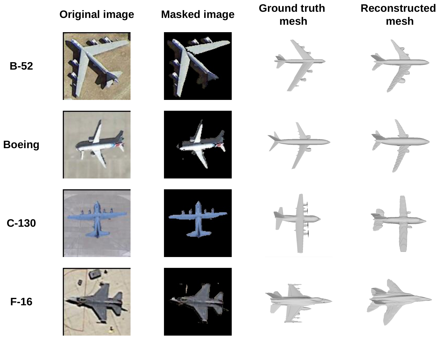
Figure 13.
The reconstruction results of the remote sensing images compared with the models of the corresponding aircraft.
Figure 13.
The reconstruction results of the remote sensing images compared with the models of the corresponding aircraft.
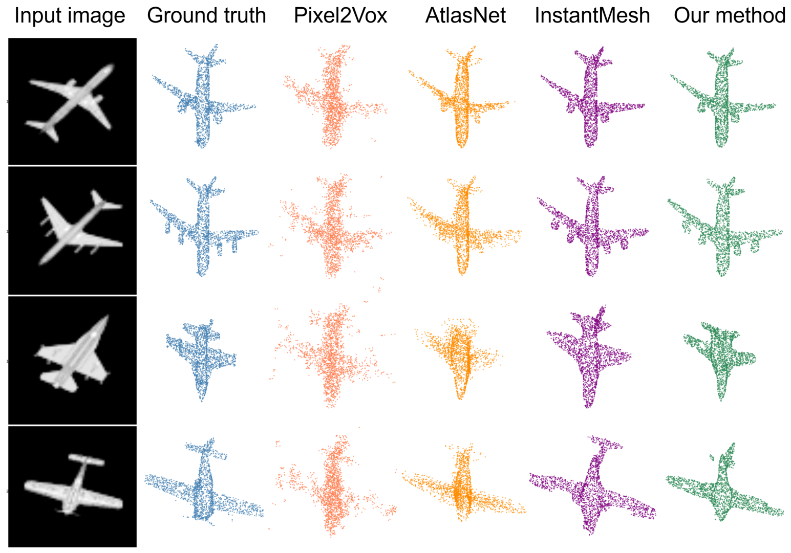
Figure 14.
The comparison of the reconstruction effects between our method and the baseline on the simulated image dataset.
Figure 14.
The comparison of the reconstruction effects between our method and the baseline on the simulated image dataset.
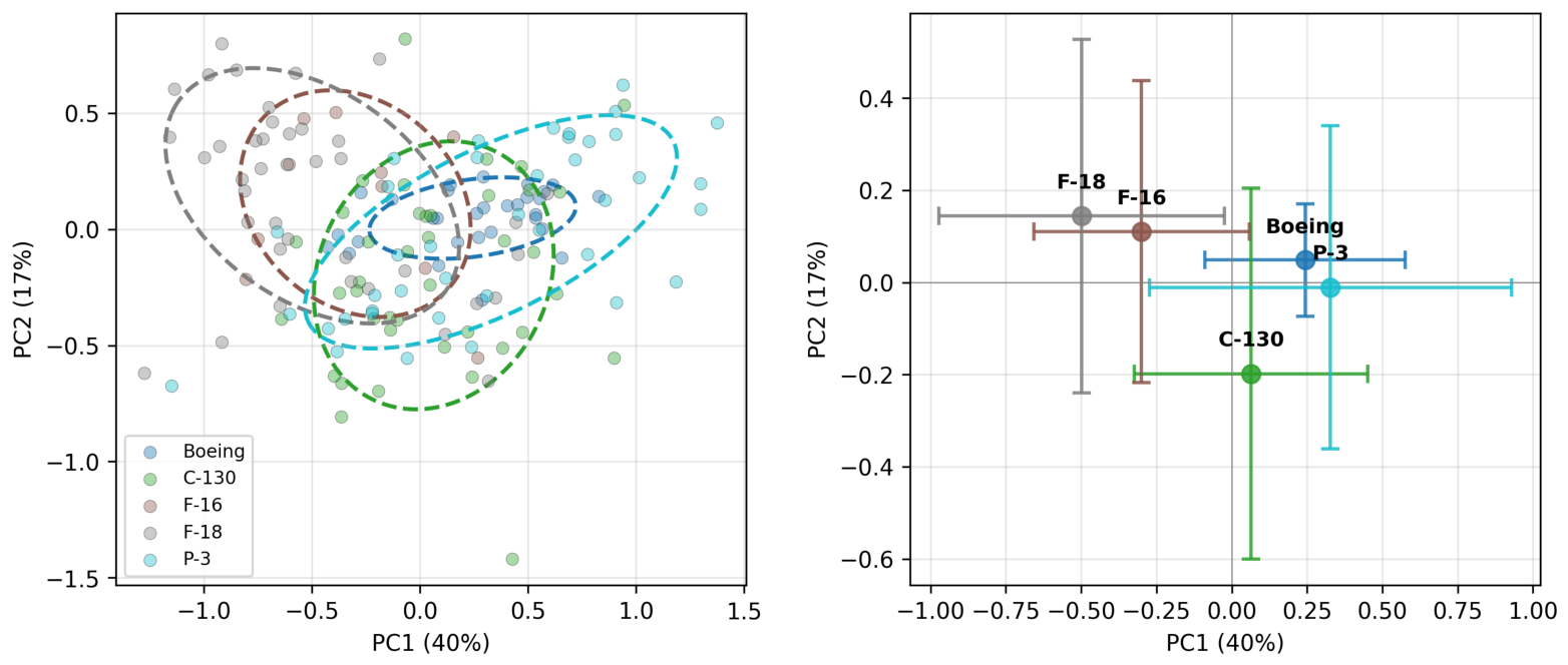
Figure 15.
Cluster analysis of the latent vectors of some samples in the reconstruction results.
Figure 15.
Cluster analysis of the latent vectors of some samples in the reconstruction results.
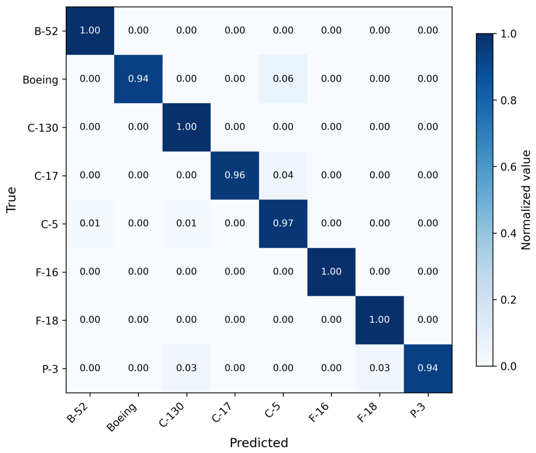
Figure 16.
Confusion matrix for our aircraft target classification method.
Figure 16.
Confusion matrix for our aircraft target classification method.
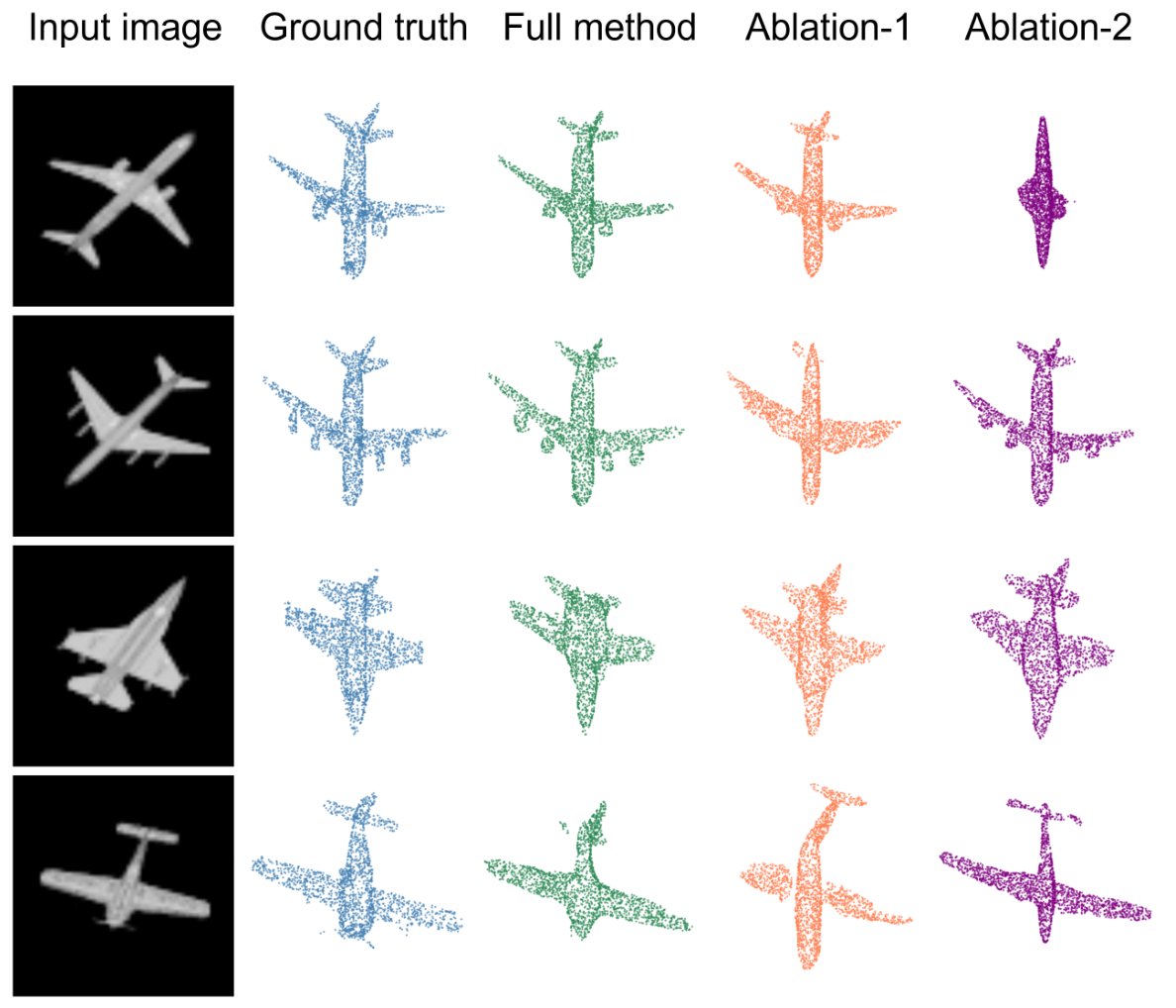
Figure 17.
Ablation study on the proposed single-view optimization pipeline. Each row shows a different test sample. From left to right: input image, ground truth, reconstruction results from the full method, ablation without dual-kernel rendering (Abl-1) and ablation without clustering prior (Abl-2).
Figure 17.
Ablation study on the proposed single-view optimization pipeline. Each row shows a different test sample. From left to right: input image, ground truth, reconstruction results from the full method, ablation without dual-kernel rendering (Abl-1) and ablation without clustering prior (Abl-2).
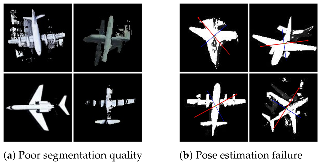
Figure 18.
Failure case analysis. (a) Samples with inaccurate input silhouettes caused by segmentation artifacts lead to degraded reconstruction quality. (b) Samples where the pose pre-estimation stage fails to find a reasonable initial alignment, resulting in severely distorted or misoriented reconstructions. The red lines represent the first principal component direction and the blue lines indicate its orthogonal direction.
Figure 18.
Failure case analysis. (a) Samples with inaccurate input silhouettes caused by segmentation artifacts lead to degraded reconstruction quality. (b) Samples where the pose pre-estimation stage fails to find a reasonable initial alignment, resulting in severely distorted or misoriented reconstructions. The red lines represent the first principal component direction and the blue lines indicate its orthogonal direction.
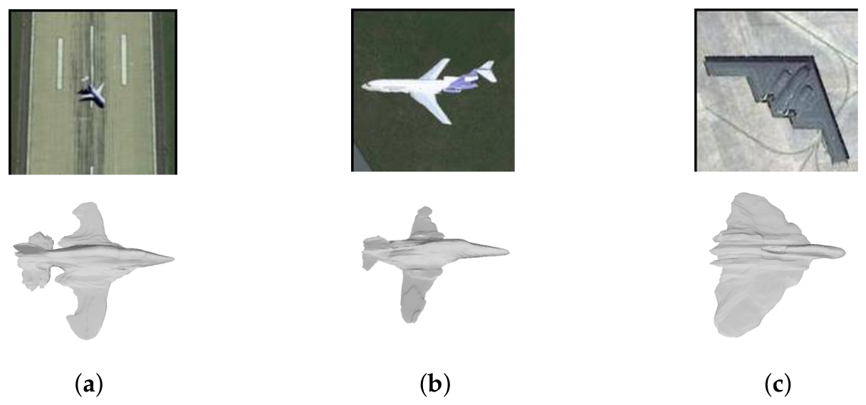
Figure 19.
Failure case analysis. Each pair shows the input silhouette and the corresponding reconstruction. (a) When the resolution of the target in the image is extremely low, it may be difficult to generate a high-quality reconstruction model. (b) A large off-nadir angle severely violates the orthographic projection assumption of the renderer, leading to inaccurate pose estimation and geometric distortion. (c) Aircraft types rarely seen in the training set of the SDF decoder produce incomplete or distorted shapes. For example, the B-2 bomber shown in the picture.
Figure 19.
Failure case analysis. Each pair shows the input silhouette and the corresponding reconstruction. (a) When the resolution of the target in the image is extremely low, it may be difficult to generate a high-quality reconstruction model. (b) A large off-nadir angle severely violates the orthographic projection assumption of the renderer, leading to inaccurate pose estimation and geometric distortion. (c) Aircraft types rarely seen in the training set of the SDF decoder produce incomplete or distorted shapes. For example, the B-2 bomber shown in the picture.
Table 1.
Quantitative reconstruction comparison with Pix2Vox on the simulated dataset. Best results in bold. ↑ and ↓ indicate higher and lower values are preferred, respectively.
Table 1.
Quantitative reconstruction comparison with Pix2Vox on the simulated dataset. Best results in bold. ↑ and ↓ indicate higher and lower values are preferred, respectively.
| ID | F-Score (↑) | CD () | NC (↑) |
|---|
|
Pix2Vox
|
Ours
|
Pix2Vox
|
Ours
|
Pix2Vox
|
Ours
|
|---|
| 1 | 0.2788 | 0.6583 | 100.7 | 37.6 | 0.5588 | 0.8499 |
| 2 | 0.2427 | 0.5292 | 127.7 | 55.9 | 0.5319 | 0.7258 |
| 3 | 0.3297 | 0.6939 | 88.8 | 33.6 | 0.5876 | 0.8434 |
| 4 | 0.2358 | 0.4800 | 130.9 | 52.2 | 0.5474 | 0.6477 |
| 5 | 0.2288 | 0.7211 | 108.0 | 33.0 | 0.5367 | 0.8364 |
| 6 | 0.1968 | 0.3153 | 116.6 | 76.4 | 0.5328 | 0.6954 |
| Mean | 0.2521 | 0.5663 | 112.1 | 48.1 | 0.5492 | 0.7665 |
Table 2.
Quantitative reconstruction comparison with AtlasNet on the simulated dataset. Best results in bold. ↑ and ↓ indicate higher and lower values are preferred, respectively.
Table 2.
Quantitative reconstruction comparison with AtlasNet on the simulated dataset. Best results in bold. ↑ and ↓ indicate higher and lower values are preferred, respectively.
| ID | F-Score (↑) | CD () | NC (↑) |
|---|
|
AtlasNet
|
Ours
|
AtlasNet
|
Ours
|
AtlasNet
|
Ours
|
|---|
| 1 | 0.6196 | 0.6583 | 39.7 | 37.6 | 0.8458 | 0.8499 |
| 2 | 0.5918 | 0.5292 | 41.4 | 55.9 | 0.6950 | 0.7258 |
| 3 | 0.5971 | 0.6939 | 40.9 | 33.6 | 0.8131 | 0.8434 |
| 4 | 0.3494 | 0.4800 | 55.1 | 52.2 | 0.6536 | 0.6477 |
| 5 | 0.5316 | 0.7211 | 45.8 | 33.0 | 0.8200 | 0.8364 |
| 6 | 0.3384 | 0.3153 | 60.5 | 76.4 | 0.7333 | 0.6954 |
| Mean | 0.5046 | 0.5663 | 47.2 | 48.1 | 0.7601 | 0.7665 |
Table 3.
Quantitative reconstruction comparison with InstantMesh on the simulated dataset. Best results in bold. ↑ and ↓ indicate higher and lower values are preferred, respectively.
Table 3.
Quantitative reconstruction comparison with InstantMesh on the simulated dataset. Best results in bold. ↑ and ↓ indicate higher and lower values are preferred, respectively.
| ID | F-Score (↑) | CD () | NC (↑) |
|---|
|
InstantMesh
|
Ours
|
InstantMesh
|
Ours
|
InstantMesh
|
Ours
|
|---|
| 1 | 0.4520 | 0.6583 | 39.3 | 37.6 | 0.8550 | 0.8499 |
| 2 | 0.4088 | 0.5292 | 59.1 | 55.9 | 0.7170 | 0.7258 |
| 3 | 0.8248 | 0.6939 | 32.7 | 33.6 | 0.8285 | 0.8434 |
| 4 | 0.4616 | 0.4800 | 43.8 | 52.2 | 0.7317 | 0.6477 |
| 5 | 0.7288 | 0.7211 | 35.0 | 33.0 | 0.8375 | 0.8364 |
| 6 | 0.1296 | 0.3153 | 106.9 | 76.4 | 0.6185 | 0.6954 |
| Mean | 0.5008 | 0.5663 | 52.8 | 48.1 | 0.7647 | 0.7665 |
Table 4.
MTARSI dataset distribution across 8 aircraft categories.
Table 4.
MTARSI dataset distribution across 8 aircraft categories.
| Category | Training | Test | Total |
|---|
| B-52 | 192 | 48 | 240 |
| Boeing | 192 | 48 | 240 |
| C-130 | 288 | 72 | 360 |
| C-17 | 192 | 48 | 240 |
| C-5 | 288 | 72 | 360 |
| F-16 | 224 | 56 | 280 |
| F-18 | 192 | 48 | 240 |
| P-3 | 128 | 32 | 160 |
| Total | 1696 | 424 | 2120 |
Table 5.
Classification performance comparison on MTARSI. Metrics: Accuracy (%), Precision (%), Recall (%), F1-Score.
Table 5.
Classification performance comparison on MTARSI. Metrics: Accuracy (%), Precision (%), Recall (%), F1-Score.
| Method | Acc. (%) | Prec. (%) | Rec. (%) | F1 |
|---|
| ResNet-18 | 93.77 ± 1.53 | 91.96 | 91.41 | 0.916 |
| YOLOv11n-cls | 96.04 ± 2.18 | 96.47 | 96.01 | 0.962 |
| ViT-Base | 96.42 ± 1.51 | 96.40 | 95.45 | 0.959 |
| EfficientNetV2-S | 97.55 ± 0.72 | 97.86 | 97.36 | 0.975 |
| RSMamba | 95.85 ± 0.37 | 96.04 | 95.73 | 0.958 |
| EAM | 95.34 ± 0.72 | 95.67 | 95.50 | 0.955 |
| Ours | 97.88 ± 0.9 | 98.38 | 97.57 | 0.979 |
Table 6.
Ablation study: contribution of the dual-kernel rendering strategy to reconstruction quality. ↑ and ↓ indicate higher and lower values are preferred, respectively.
Table 6.
Ablation study: contribution of the dual-kernel rendering strategy to reconstruction quality. ↑ and ↓ indicate higher and lower values are preferred, respectively.
| Configuration | CD () | F-Score (↑) | NC (↑) |
|---|
| Full method | 4.24 | 0.688 | 0.756 |
| W/o dual-kernel rendering | 5.53 | 0.578 | 0.739 |
| Degradation | +1.29 (30.4%) | −0.110 (16.0%) | −0.017 (2.1%) |
Table 7.
Ablation study: contribution of the clustering prior to reconstruction quality. ↑ and ↓ indicate higher and lower values are preferred, respectively.
Table 7.
Ablation study: contribution of the clustering prior to reconstruction quality. ↑ and ↓ indicate higher and lower values are preferred, respectively.
| Configuration | CD () | F-Score (↑) | NC (↑) |
|---|
| Full method | 4.24 | 0.688 | 0.756 |
| W/o clustering prior | 7.65 | 0.464 | 0.743 |
| Degradation | +3.41 (80.4%) | −0.224 (32.5%) | −0.013 (1.7%) |
Table 8.
Ablation study: contribution of the reconstruction feature branch to classification accuracy.
Table 8.
Ablation study: contribution of the reconstruction feature branch to classification accuracy.
| Configuration | Acc. (%) | Prec. (%) | Rec. (%) | F1 |
|---|
| Image backbone only | 96.7 ± 1.2 | 97.19 | 96.53 | 0.968 |
| Feature fusion method (proposed) | 97.88 ± 0.8 | 98.38 | 97.57 | 0.979 |
| Improvement | +1.18 | +1.19 | +1.04 | +0.011 |
Table 9.
Specifications of the key components.
Table 9.
Specifications of the key components.
| Component | Parameter | Value |
|---|
| SDF decoder | Architecture | 6-layer MLP: |
| Latent dim K | 8 |
| Regularization | dropout 0.3 |
| Params | ∼0.80 M |
| Training | Optimizer | Adam, lr → linear decay |
| Batch/Epochs | 64 shapes/2500 |
| Hardware | Single RTX 4090, ∼24 h |
| Phase I | Density kernel | Logistic with learnable , init 10.0 |
| Optimized vars | Latent z, translation t, pose |
| Steps/Batch | 500/ rays per step |
| Learning rates | 5 × 10⁻³, |
| Phase II | Density kernel | Laplace with learnable , init 0.01 |
| Optimized vars | Latent z |
| Steps | 2000/ rays per step |
| Learning rates | |
| Scheduler | ReduceLROnPlateau (factor 0.8, patience 500) |
| Termination | stop when LR |
| Mesh extraction | Algorithm | Marching Cubes, grid |
| Max batch | points |
Table 10.
Computational cost of the single-view optimization pipeline per input image.
Table 10.
Computational cost of the single-view optimization pipeline per input image.
| Component | MLP Calls | MACs | FLOPs |
|---|
| Phase 1 decoder | 65,536,000 | 52,059,701,248,000 | 104,119.40 GFLOPs |
| Phase 2 decoder | 262,144,000 | 208,238,804,992,000 | 416,477.61 GFLOPs |
| Post-processing | 2,560,000 rays | — | 3.28 GFLOPs |
| Total | 327,680,000 | — | 520,600.29 GFLOPs |
Table 11.
GPU memory footprint of the single-view optimization pipeline per input image. All values are measured under FP32 precision with batch size 1024 rays.
Table 11.
GPU memory footprint of the single-view optimization pipeline per input image. All values are measured under FP32 precision with batch size 1024 rays.
| Component | Memory (MB) | Proportion |
|---|
| Model parameters (FP32) | 3.05 | 0.3% |
| Resident data † | 0.53 | <0.1% |
| Per-step activation (Phase 1 & 2) | 1152.5 | 97.7% |
| Decoder layer outputs | 1035.5 | 87.8% |
| Input buffers | 11.0 | 0.9% |
| Render temporaries | 6.0 | 0.5% |
| Adam optimizer states | 6.1 | 0.5% |
| CUDA context overhead | ∼20 | 1.7% |
| Peak (batch) | 1179.2 | 100% |
| Mesh extraction (no-grad) | ∼2327 | — |




 ,
,