Article

Long-Horizon Mining Subsidence Forecasting and Ecological Time-Lag Assessment Using Multi-Source Remote Sensing

1
Engineering Technology Innovation Center for Ecological Protection and Restoration in the Middle Yellow River, Ministry of Natural Resources, Taiyuan 030024, China
2
Key Laboratory of Ionic Rare Earth Resources and Environment, Ministry of Natural Resources of the People’s Republic of China, Ganzhou 341000, China
3
College of Geological and Surveying Engineering, Taiyuan University of Technology, Taiyuan 030024, China
4
Shanxi Geological Environment Monitoring and Ecological Restoration Center, Taiyuan 030024, China
*
Author to whom correspondence should be addressed.
These authors contributed equally to this work.
Remote Sens. 2026, 18(16), 2829; https://doi.org/10.3390/rs18162829
Submission received: 2 July 2026 / Revised: 12 August 2026 / Accepted: 17 August 2026 / Published: 20 August 2026

Highlights

What are the main findings?
  • The N-BEATS model, utilizing a Multi-Input Multi-Output (MIMO) strategy, effectively mitigates temporal error cascades, demonstrating superior stability in 15-step long-horizon subsidence extrapolation compared to traditional recursive models.
  • Mining-induced ecological degradation exhibits a distinct “center-edge” spatiotemporal mismatch: immediate deterioration at the collapse core (Lag 0) and a hidden 1–2 year lag at the peripheral basin.
What are the implications of the main findings?
  • Overcoming spatial sampling bias and cumulative forecasting errors provides a reliable early-warning framework for long-term, proactive safety management in complex geological environments.
  • Quantifying the “pseudo-stable” hidden degradation period in optical indicators enables more scientifically precise, full-cycle tracking and proactive restoration of mining-disturbed ecosystems.

Abstract

Surface deformation induced by underground coal mining is characterized by strong nonlinearity and spatial heterogeneity, which complicates early warning and ecological assessment. While InSAR-driven data assimilation models and remote sensing-based ecological indices are widely used for long-term monitoring, three fundamental limitations remain unresolved: (1) severe spatial imbalance in deformation samples biases data-driven models toward mean-reverting predictions, (2) recursive multi-step forecasting accumulates errors, leading to instability in long-horizon extrapolation, and (3) in ecological monitoring, vegetation resilience further induces a multi-year observation lag, resulting in a “pseudo-stable” bias in optical indicators. To address these issues, this study proposes an unified framework integrating multi-step deformation prediction and ecological time-lag analysis. Taking the Datong Coalfield as the study area, we utilized 231 Sentinel-1A images from March 2017 to December 2024 for SBAS-InSAR deformation inversion. A spatial stratified sampling strategy is used to extract 5894 representative points. A 24-step backward and 15-step forward windows were reconstructed to systematically compare six predictive models. Simultaneously, the Remote Sensing Ecological Index (RSEI) derived from Landsat data is used for cross-lagged analysis. The results demonstrate that: (1) The maximum deformation rate reached −276.75 mm/year, with cumulative subsidence exceeding −2000 mm. (2) At 3-step short-term forecasting, all models proved robust, with LSTM performing best (RMSE = 5.78 mm). At 15-step extreme extrapolation, however, traditional recursive models diverged significantly (Kalman, RMSE = 45.70 mm), whereas N-BEATS maintained stability and effectively mitigated temporal error cascades with an RMSE of 17.98 mm. (3) The core collapse zone exhibited concurrent ecological degradation (Lag 0), while the marginal basin presented a hidden degradation period of one to two years. It provides reliable scientific support for precise tracking and proactive safety management in complex mining areas.

1. Introduction

High-intensity underground coal mining inevitably triggers the movement and failure of overlying rock strata. This subsequently leads to large-scale surface deformation and subsidence disasters. Such events directly threaten the operational safety of mining infrastructure and surface structures. Furthermore, they profoundly reshape surface hydrology and vegetation habitats, posing a severe challenge to regional ecological quality [1,2]. In typical high-intensity multi-seam mining areas, the surface subsidence field generally exhibits pronounced nonlinearity and spatial heterogeneity [3]. This phenomenon is primarily driven by complex geological environments and overlapping disturbances from historical mined-out areas. Deformation basins in these mining regions frequently demonstrate highly polarized spatial characteristics. Their peripheral margins are typically extensive and characterized by gradual subsidence. Conversely, the active mining cores are often accompanied by intense and sudden nonlinear collapse and surface fracturing [4]. Ultimately, these complex spatiotemporal dynamics present immense challenges to traditional disaster prevention systems. They also significantly hinder the proactive management and restoration of the mining ecological environment.
Given these complex and severe nonlinear dynamics, precisely tracking the trajectory of surface deformation is the primary prerequisite for constructing proactive disaster prevention systems. Interferometric Synthetic Aperture Radar (InSAR) technology demonstrates distinct advantages in the dynamic surface monitoring of mining areas. This is due to its independence from illumination and meteorological constraints. The advancement of time-series InSAR methods has enabled a clearer characterization of the cumulative impacts of underground mining on the surface [5,6,7]. Building upon this, integrating data-driven algorithms to construct time-series forecasting models has emerged as a prominent research direction for early deformation warning. Deep learning algorithms, particularly Long Short-Term Memory (LSTM) networks, have been widely adopted. They demonstrate significant potential in modeling nonlinear deformation characteristics [8]. However, existing predictive frameworks still confront two critical bottlenecks when addressing the specific evolutionary patterns of complex mining areas. Spatially, the deformation field is overwhelmingly dominated by relatively stable background points. Consequently, global models are highly susceptible to “mean reversion” during optimization. This limitation often leads to an underestimation of the extreme collapse trends within the active mining core [9,10]. Temporally, current mainstream algorithms predominantly employ single-step recursive strategies for multi-step forward extrapolation. These models rely heavily on the iterative feedback of intermediate predicted states. As the forecasting horizon extends, this mechanism frequently triggers systematic error cascade amplification. This divergence fails to meet the stringent accuracy requirements for long-term safety warnings [11,12]. Therefore, current surface deformation forecasting in mining regions urgently requires novel approaches. It is imperative to overcome the mean reversion limitations induced by spatial heterogeneity and to mitigate the error cascade processes inherent in long-horizon predictions.
Beyond focusing on surface deformation evolution, investigating the disturbance mechanisms of high-intensity mining on surface ecosystems represents another core dimension. This is essential for comprehensively evaluating the geological and environmental effects within mining regions. Traditionally, environmental management in mining areas has heavily depended on optical remote sensing for post-event ecological quality monitoring. Previous studies have attempted to integrate surface deformation data as structural constraints within ecological evaluation frameworks. This approach aims to enhance the adaptability of monitoring results to specific mining environments [13,14]. However, extended time-series observations reveal that the propagation of underground mining disturbances to surface ecosystems is rarely instantaneous. Surface vegetation possesses intrinsic drought resilience, while deep soil moisture undergoes a progressive depletion process. These combined factors generate substantial spatiotemporal misalignments and cross-lagged effects between underlying surface deformation and superficial ecological degradation [15,16]. This ecological “hidden degradation period” can persist for months or even years. It objectively reflects the profound complexity of ecological evolution within these mining contexts [17]. Therefore, it is crucial to quantitatively elucidate the time-lag mechanisms between deformation and remote sensing ecological quality at the pixel scale. This analysis holds significant independent value for scientifically interpreting the full-cycle dynamics of mining-induced ecological degradation.
To address these issues, this study relies on long-term multi-source remote sensing data. We conduct prospective multi-step forecasting of surface deformation and an in-depth analysis of ecological evolution mechanisms. For deformation prediction, existing models are constrained by both spatial imbalance and temporal cascade errors. To overcome this dual bottleneck, we introduce a spatial stratified heterogeneous sampling strategy. This allows us to construct an unbiased time-series dataset. Furthermore, we apply the N-BEATS model, which features multi-input multi-output (MIMO) direct mapping capabilities. We conduct multi-step forward benchmark testing against traditional statistical and classical machine learning models. These baseline models include Autoregressive Integrated Moving Average (ARIMA), Kalman, Random Forest (RF), Extreme Gradient Boosting (XGBoost), and LSTM. The objective is to identify a reliable early warning scheme capable of suppressing long-sequence blind-test errors. In the ecological dimension, we construct a spatial cross-lagged model. This is based on the Remote Sensing Ecological Index (RSEI) and Small Baseline Subset InSAR (SBAS-InSAR) deformation sequences. The model precisely delineates the spatiotemporal misalignment and lag characteristics between physical surface collapse and superficial ecological degradation at the pixel scale.

2. Study Area and Data

2.1. Study Area

The study area (Figure 1) is located within the Datong Coalfield in northern Shanxi Province (112.56°E–113.42°E, 39.73°N–40.22°N). It is situated within the transitional zone between the Loess Plateau and the alluvial plain of the Datong Basin. The regional topography is generally elevated in the northwest and lower in the southeast, with an average elevation of approximately 1279 m. Furthermore, the regional surface is widely covered by Quaternary Middle and Upper Pleistocene loess. This specific loess formation is characterized by well-developed vertical joints, high porosity, and strong collapsibility. Consequently, the surface structure exhibits an exceptionally high sensitivity to mechanical disturbances induced by deep coal seam mining [18].
This region is characterized by a typical north temperate, semi-arid continental monsoon climate. Specifically, meteorological statistics from 2017 to 2024 indicate a mean annual temperature of 7.2 °C and a mean annual precipitation of 559.7 mm. Governed by inland air masses and local topography, the area experiences four distinct seasons and an arid climate. It exhibits pronounced characteristics of seasonal drought. The annual potential evapotranspiration significantly exceeds actual precipitation, resulting in a severe moisture deficit. Constrained by these natural hydrothermal conditions, the ecological baseline of the mining area is inherently fragile. Soil moisture content is generally low. The surface vegetation is predominantly composed of drought-tolerant temperate shrubs, desertified herbs, and sparse artificial coniferous forests. Consequently, the ecosystem’s natural resistance to disturbances and its intrinsic capacity for self-restoration are considerably limited [19].
The Datong Coalfield is a representative large-scale energy base in China. Within this region, Jurassic and Permo-Carboniferous coal seams occur in vertical superposition. This configuration constitutes a typical dual-system composite mining area. The area hosts multiple modern, ultra-large underground mines. Prominent examples include the Tashan, Tongxin, Yanzishan, and Majiliang collieries. These mines generally employ fully mechanized longwall mining techniques characterized by high cutting heights and rapid advancement. The long-term, high-intensity extraction of multiple seams disrupts the original mechanical equilibrium of the overlying strata. Consequently, deep geological disturbances propagate continuously upward [20]. Ultimately, this triggers extensive discontinuous surface damage. Such damage manifests as subsidence basins, boundary collapse funnels, and penetrating ground fissures [21].

2.2. Data

The data sources for this study primarily comprise radar imagery for surface deformation inversion, auxiliary spatial data, and optical remote sensing imagery for ecological assessment.
For surface deformation monitoring, 231 Sentinel-1A Single Look Complex (SLC) images covering the Datong Coalfield were collected from March 2017 to December 2024 [22]. This dataset was acquired using the Interferometric Wide (IW) swath mode and vertical-vertical (VV) polarization. The azimuth and radar incidence angles are 346.5° and 35.5°, respectively. To effectively mitigate baseline estimation errors, Precise Orbit Ephemeris (POE) data provided by the European Space Agency (ESA) were incorporated to improve orbit determination accuracy [23]. Concurrently, the 30 m Shuttle Radar Topography Mission (SRTM) Digital Elevation Model (DEM) from the United States Geological Survey (USGS) was used for facilitating topographic phase simulation and geocoding [24]. To validate the accuracy of the inversion results, continuous Global Navigation Satellite System (GNSS) observations from the SXDT station (marked in Figure 1) were acquired from the Earthquake Data Science Center (EDSC) [25]. Furthermore, to mitigate the effects of tropospheric delay, this study introduced high-resolution delay products during the interferogram generation step. These were derived from the Generic Atmospheric Correction Online Service (GACOS) [26,27]. This system utilizes meteorological data from the European Centre for Medium-Range Weather Forecasts (ECMWF) and DEMs as its foundation. It also integrates GNSS observation data to assist in the calculation. It computes the Zenith Total Delay (ZTD) within the study area. Through elevation fitting and iterative filtering, it separates the strongly topography-correlated stratified delay, and extracts the turbulent delay via spatial differencing. The resulting high-resolution zenith delay products are subsequently projected into the radar line-of-sight (LOS) direction. This enables the precise correction of atmospheric phase biases within the interferograms.
Regarding ecological quality assessment, optical imagery from the Landsat series spanning 2017 to 2024 was simultaneously used. To minimize the interference of seasonal phenological changes on ecological evaluations, imagery from the annual vegetation growing season (June to September) was strictly selected. This served as the assessment baseline. During the preprocessing phase, cloud masking and pixel-level median synthesis algorithms were applied. This ultimately yielded eight high-quality and cloud-free composite images, with one image generated for each year [28,29].

3. Methods

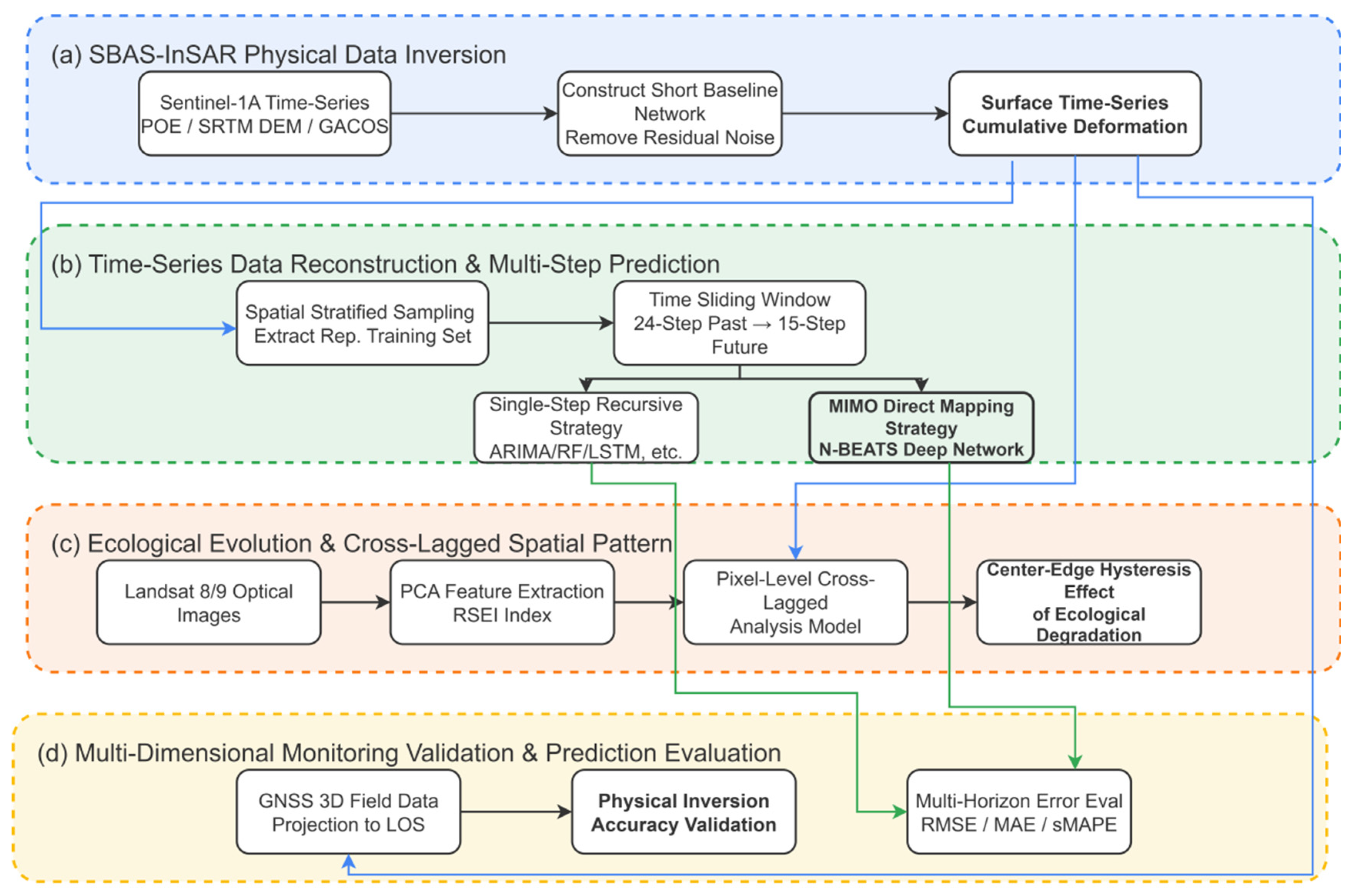
The long-term multi-step forecasting and deformation–ecology framework developed in this study is illustrated in Figure 2. Section 3.1 first introduces the SBAS-InSAR deformation monitoring method. Section 3.2 then describes the time-series data reconstruction procedure and multi-step forecasting strategy. Section 3.3 examines the ecological evolution characteristics of the mining area and the spatial patterns revealed by cross-lagged analysis. Finally, Section 3.4 presents the methods for multi-dimensional validation of monitoring accuracy and evaluation of forecasting performance.

3.1. SBAS-InSAR

The SBAS-InSAR technique was originally introduced by Berardino et al. [30] in 2002. This methodology constructs an interferometric network by imposing strict spatiotemporal baseline thresholds. The primary objective of this constraint is to effectively suppress spatial decorrelation and mitigate residual topographic errors.
Suppose that  N + 1  SAR images covering the identical region are acquired throughout the study period. The corresponding acquisition time series is denoted as  T 0 , T 1 , . . . , T n . An image with an optimally centered spatiotemporal baseline is selected as the common master image. Subsequently, the remaining slave images undergo radiometric calibration and precise geometric coregistration. This procedure utilizes POE data and an external DEM to guarantee sub-pixel alignment across all images. By establishing appropriate temporal and spatial baseline thresholds, image pairs satisfying these criteria are systematically combined. Consequently, the total number of generated differential interferograms, denoted as  M , satisfies the following constraint:
N + 1 2 M N ( N + 1 ) 2
Assuming  T 0  serves as the initial temporal reference for zero deformation, let us examine an arbitrary pixel  x . Consider its representation within the  k -th differential interferogram, which is generated through the interference of SAR images acquired at times  T A  and  T B  (where  T A < T B ). The resulting unwrapped differential interferometric phase, denoted as  δ φ x , k , can be:
δ φ x , k = φ x ( T B ) φ x ( T A ) = δ φ d e f , x , k + δ φ t o p o , x , k + δ φ a t m , x , k + δ φ o r b , x , k + δ φ n o i s e , x , k
where  δ φ d e f , x , k  represents the true deformation phase in the radar LOS direction;  δ φ t o p o , x , k  denotes the residual topographic phase caused by the limited accuracy of the external DEM; and  δ φ a t m , x , k  indicates the phase error induced by tropospheric atmospheric delay. Furthermore,  δ φ o r b , x , k  represents the residual satellite orbital phase resulting from baseline estimation errors, while  δ φ n o i s e , x , k  signifies the noise phase attributed to system thermal noise and spatiotemporal decorrelation.
Specifically, the true deformation phase in the LOS direction is functionally related to the radar wavelength  λ  and the cumulative deformation  d x ( T )  during this period. This relationship is expressed by the following equation:
δ φ d e f , x , k = 4 π λ [ d x ( T B ) d x ( T A ) ]
To mitigate the interference of tropospheric delay on deformation signals, this study incorporates tropospheric zenith delay products from the GACOS during the interferogram generation phase. This facilitates the precise atmospheric delay correction of the unwrapped phase. Prior to the inversion process,  δ φ a t m , x , k  is systematically isolated and removed. Concurrently, selected Ground Control Points (GCPs) are utilized for orbital refinement to eliminate residual phases. Through these procedures, Equation (2) can be simplified into a matrix form that predominantly represents the LOS deformation:
δ φ = A d
where  δ φ  represents the  M × 1  dimensional observation vector of the differential interferometric phase;  d  denotes the  ( N + 1 ) × 1  dimensional vector of the unknown cumulative deformation at each observation time; and  A  is the  M × ( N + 1 )  dimensional coefficient matrix.
During the inversion process, strict spatiotemporal baseline limits may cause the interferometric network to degrade into multiple isolated short-baseline subsets. Consequently, the coefficient matrix will experience rank deficiency. This phenomenon renders the traditional least-squares method incapable of a direct solution. Therefore, this study employs Singular Value Decomposition (SVD) to compute the pseudo-inverse of the coefficient matrix. This approach facilitates the collaborative adjustment of multiple independent short-baseline subsets. Finally, the least-squares solution for the deformation velocity is obtained under the minimum norm criterion. Through temporal integration, the continuous time-series cumulative deformation for spatial points is then systematically extracted.

3.2. Construction of the Time-Series Multi-Step Forecasting Model

3.2.1. Construction of the Time-Series Modeling Dataset

Coherent points in mining areas derived from SBAS-InSAR inversion often exhibit massive and extremely imbalanced spatial distributions. A vast amount of stable background point clouds easily causes deep learning models to fall into the “mean reversion” trap during global optimization. This consequently leads to a severe underestimation of the evolutionary trends in extreme collapse zones. To construct an unbiased time-series training set, this study introduces a spatial stratified heterogeneous sampling strategy [31]. Specifically, to isolate true physical subsidence from stable background phase noise, coherent points with a deformation rate greater than −30 mm/year are first excluded. Differentiated grid thinning is then applied to varying deformation regions. In the peripheral basin areas with gentle deformation, large-scale grids are utilized for heavy downsampling. As the deformation gradient increases, the grid scale is progressively reduced. Conversely, in the severe collapse core zones, micro-grids are employed to maintain high-density retention. Within each spatially discrete grid, extreme feature points exhibiting the maximum subsidence rate (maximum absolute value) are strictly extracted and retained. Through this dimensionality reduction strategy, this study aims to filter a high-quality, representative point set from the massive regional point cloud. This set effectively balances the globally stable background with extreme disaster characteristics. Consequently, it mitigates spatial imbalance and establishes a reliable data foundation for evaluating the subsequent models’ robustness in capturing nonlinear mutations. Compared to conventional uniform or random sampling approaches, this strategy effectively avoids overwhelming the models with redundant stable points, which typically leads to the underfitting of extreme values [9,10]. It also prevents the erroneous smoothing of peak subsidence values in the collapse core, ensuring a balanced feature representation for global deep learning models.

3.2.2. Data Preprocessing and Multi-Model Prediction Strategies

Prior to model training, this study standardized the InSAR sequences of high-quality points extracted in Section 3.2.1. This process utilized the Python-based darts time-series framework [32]. Occasional missing values in the raw sequences were filled via linear interpolation. The sequences were then resampled to a fixed 12-day step.
To ensure deep network numerical stability, each sequence was mapped to a [0, 1] feature space. This was achieved using Min-Max normalization. To strictly prevent data leakage, the final 15 steps (180 days) of all point sequences were reserved as the blind-test validation set. The remaining preceding sequences served as the training set. Model inputs were reconstructed using a sliding window technique. The forward prediction window was set to 15 steps, as preliminary testing indicated that prediction errors become excessively dispersed beyond this horizon. The historical look-back step was set to 24 steps (288 days) to encompass a near-complete annual cycle, ensuring sufficient historical context for the models. Predictive performance was primarily evaluated at five characteristic nodes: 3, 6, 9, 12, and 15 steps. Operationally, the six comparative algorithms were divided into two prediction strategies: (1) Single-step recursive strategy: ARIMA [33] and Kalman [34] acted as local models for point-wise adaptive fitting. Conversely, RandomForest (RF) [35], XGBoost [36], and LSTM [37] functioned as global models. These models only map future single-step predictions and iteratively feed them back. Highly dependent on intermediate states, this mechanism easily causes cumulative error divergence during long-sequence extrapolation. (2) MIMO strategy: The N-BEATS [38] network adopted this mechanism. Its output chunk length directly aligned with the blind-test window. It utilized 24-step historical features to output a 15-step parallel prediction vector simultaneously. Bypassing cyclic feedback, this mechanism fundamentally severed the temporal cascading propagation of errors.
All deep networks were collectively trained for 50 epochs. They utilized MSE loss, the Adam optimizer, and GPU acceleration. Ultimately, the prediction vectors underwent inverse un-normalization to restore true displacement values. All models completed systematic hyperparameter optimization on the validation set using a Grid Search strategy. Their final optimal core hyperparameter configurations are detailed in Table 1.

3.3. Ecological Quality Assessment and Deformation Cross-Lagged Analysis in Mining Areas

This section aims to quantitatively elucidate the spatiotemporal evolution of underground mining disturbances propagating to surface ecosystems. Furthermore, it seeks to establish a scientific foundation for prospective disaster early warning in subsequent deformation predictive modeling. To achieve this, an ecological quality index is constructed utilizing long-term optical remote sensing imagery. Building upon this foundation, a spatial cross-lagged analysis is systematically introduced. This analytical approach effectively extracts the underlying spatiotemporal response patterns between physical surface subsidence and ecological degradation.

3.3.1. Inversion of the RSEI

This research utilizes cloud-free Landsat 8/9 OLI/TIRS surface reflectance imagery covering the study area. This dataset corresponds to the annual vegetation growing seasons (June to September) spanning from 2017 to 2024. From this imagery, four core components are systematically extracted. These consist of greenness (NDVI), wetness (WET), dryness (NDBSI), and heat (LST). Together, these parameters comprehensively reflect the inherent baseline characteristics of the surface ecosystem.
A single indicator is inherently insufficient to comprehensively characterize the complex ecological conditions within mining areas. Consequently, this study employs Principal Component Analysis (PCA) for objective data dimensionality reduction and weight allocation across the four aforementioned components [39]. The first principal component (PC1), which encapsulates the vast majority of the information variance, is subsequently extracted as the initial ecological index ( R S E I 0 ):
R S E I 0 = 1 P C A 1 ( N D V I , W E T , N D B S I , L S T )
To eliminate dimensional discrepancies across disparate years and facilitate long-term spatiotemporal comparative analysis, the initial index ( R S E I 0 ) is subjected to range standardization. This procedure linearly maps the data into a [0, 1] feature space. Ultimately, this derivation yields the final ecological index:
R S E I = R S E I 0 R S E I 0 _ m i n R S E I 0 _ m a x R S E I 0 _ m i n
where a  R S E I  value more closely approximating 1 signifies superior ecological quality for the corresponding spatial pixel. Conversely, a lower value denotes a prevailing state of ecological degradation and environmental impairment.

3.3.2. Extraction of the Deformation-Ecology Cross-Lagged Effect

Surface subsidence induced by underground coal mining in the Datong Coalfield is a progressive evolutionary process. This subsidence triggers overlying strata fracturing, the development of water-conducting fracture zones, groundwater table decline, and surface soil moisture loss. The subsequent impacts on vegetation physiological states, such as chlorophyll degradation and canopy wilting, do not manifest instantaneously. Consequently, this study introduces a pixel-scale cross-lagged correlation analysis. This analytical approach quantitatively extracts the temporal lag patterns between physical surface subsidence and ecological degradation [9].
Let  D ( t )  denote the cumulative surface deformation increment derived from InSAR inversion in year  t . Correspondingly, let  E ( t )  represent the optical RSEI value for that same year. We must account for the delayed resilience inherent to plant physiological succession in semi-arid regions. Furthermore, the statistical sample size is constrained by the eight-year time series spanning 2017 to 2024. Consequently, this study strictly constrains the temporal lag window, denoted as  k , to the set of {0, 1, 2} years. For any given spatial pixel, the Pearson correlation coefficient  R k  between its deformation sequence and ecological sequence at a temporal lag of  k  years is calculated as follows:
R k = t = 1 N k ( D t D ¯ ) ( E t + k E ¯ ) t = 1 N k ( D t D ¯ ) 2 t = 1 N k ( E t + k E ¯ ) 2
where  N  represents the total duration of the study period ( N = 8 ),  E t + k  denotes the ecological quality at a temporal lag of  k  years, and  D ¯  and  E ¯  signify the mean values of cumulative deformation and ecological quality, respectively, throughout the effective observational interval.
To ascertain the optimal ecological response period for localized spatial units, the temporal parameter  k  that maximizes the absolute correlation coefficient,  | R k | , is systematically extracted. This specific value is subsequently designated as the characteristic lag time,  T l a g , for the corresponding pixel:
T l a g = a r g max k { 0,1 , 2 } ( | R k | )

3.4. Monitoring Accuracy Validation and Multi-Dimensional Forecasting Evaluation

3.4.1. Validation of InSAR Monitoring Accuracy

To objectively validate the accuracy of the time-series deformation derived from SBAS-InSAR, this study incorporates concurrent three-dimensional GNSS measurement data for cross-validation. To mitigate the impact of potential geolocation uncertainties associated with coherent points, a 100 m × 100 m buffer zone was delineated. All coherent points within this specific boundary were subsequently incorporated into the accuracy validation process. Furthermore, InSAR monitoring results inherently reflect one-dimensional deformation along the radar LOS. Therefore, the three-dimensional displacements of GNSS stations must be projected onto the LOS direction. This projection is fundamentally based on the spatial geometric relationship of the side-looking radar [40]. The specific conversion formula is expressed as follows:
d L O S _ G N S S = [ cos θ sin θ cos α h sin θ sin α h ] d u d e d n
where  d L O S _ G N S S  represents the projected GNSS displacement converted to the LOS direction,  d u d e , and  d n  correspond to the vertical, east–west, and north–south components measured by GNSS, respectively,  θ  denotes the local radar incidence angle, and  α h  signifies the satellite heading angle.
Upon achieving spatial datum unification and temporal alignment, it is necessary to calculate the difference between the InSAR observations and the projected GNSS values. The corresponding formula is expressed as follows:
Δ d = d L O S _ I n S A R d L O S _ G N S S
To comprehensively quantify the error characteristics, this study employs two metrics for accuracy evaluation: Root Mean Square Error (RMSE) and Standard Deviation (STD):
R M S E = 1 n i = 1 n ( Δ d i ) 2
S T D = 1 n i = 1 n ( Δ d i μ ) 2
where  n  represents the number of validation epochs,  μ  denotes the mean error, and  Δ d i  signifies the difference between the InSAR-derived cumulative deformation and the GNSS-measured deformation at the  i -th validation epoch. The RMSE intuitively reflects the level of absolute deviation, whereas the STD is utilized to characterize the degree of error dispersion.

3.4.2. Multi-Dimensional Forecasting Evaluation

To quantitatively evaluate the deformation extrapolation performance of various predictive algorithms across distinct forward forecasting horizons (3, 6, 9, 12, and 15 steps), this study introduces three statistical metrics for a comprehensive assessment. These metrics comprise the RMSE, Mean Absolute Error (MAE), and symmetric Mean Absolute Percentage Error (sMAPE). Their respective mathematical formulas are expressed as follows:
R M S E = 1 T t = 1 T ( y t y ^ t ) 2
M A E = 1 T t = 1 T | y t y ^ t |
s M A P E = 200 % T t = 1 T | y t y ^ t | | y t | + | y ^ t |
In addition, to rigorously evaluate the statistical significance of predictive accuracy differences among models, the Diebold-Mariano (DM) test was employed. Let  e 1 , t  and  e 2 , t  denote the prediction errors of the baseline model and the proposed N-BEATS model, respectively. The loss differential  d t  based on absolute error is defined as:
d t = | e 1 , t | | e 2 , t |
The null hypothesis ( H 0 : E [ d t ] = 0 ) assumes that both models share identical forecasting accuracy. The DM test statistic is calculated as:
D M = d ¯ V ^ d / T
where  d ¯  is the sample mean of  d t  over  T  validation epochs. Crucially, given that prediction errors over an  h -step forward horizon exhibit temporal autocorrelation, the asymptotic variance  V ^ d  should be corrected using the sample autocovariance up to lag  h 1 :
V ^ d = γ ^ 0 + 2 k = 1 h 1 γ ^ k
where  γ ^ k  represents the  k -th lag autocovariance of  d t . The test was evaluated at a significance level of  α = 0.05 . Furthermore, 95% confidence intervals (CIs) for the evaluation metrics were computed via percentile bootstrapping (1000 resamples) to further verify the stability of the forecasting performance.

4. Results

4.1. Long-Term Surface Deformation Monitoring Results in the Datong Mining Area

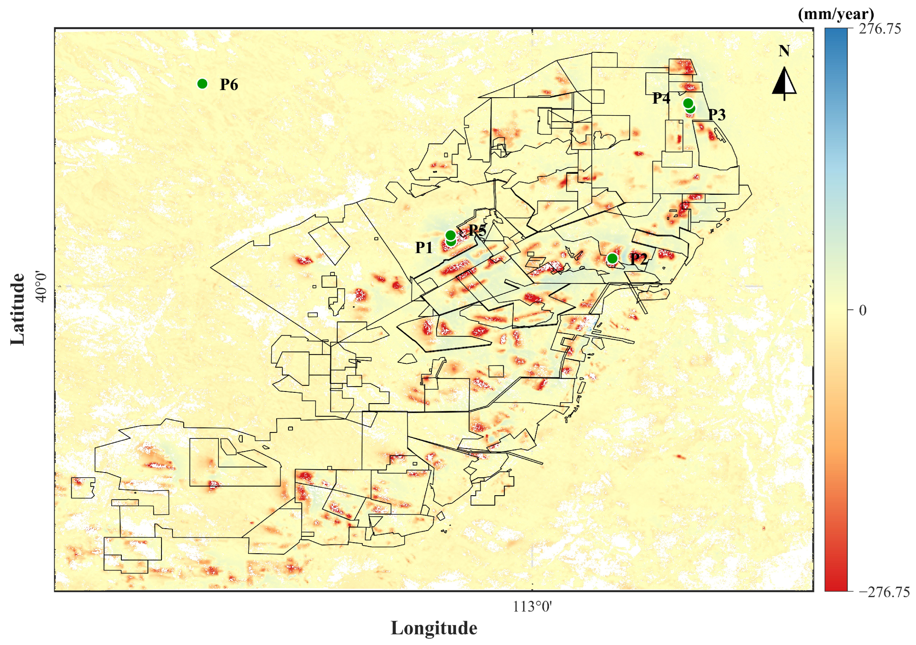
Using the data and methods separately described in Section 2.2 and Section 3.1, the long-term annual average surface deformation velocity field of the Datong Coalfield was inverted and obtained (as shown in Figure 3). Long-term monitoring results indicate that the surface of the Datong mining area exhibits extremely severe and non-stationary spatiotemporal dynamic evolution characteristics. This is primarily influenced by the disturbances from underground multi-seam and high-intensity mining operations. Spatially, the cumulative deformation basins across the entire region display a typically unbalanced distribution pattern. Macroscopically, the deformation gradients at the periphery and marginal transition zones of the coalfield are extremely gentle. The annual average deformation velocity decays smoothly from the outside inwards. These areas generally maintain a sub-stable surface state, controlled within −30 mm/year. However, as the spatial location approaches the core target area of underground mining, the spatial heterogeneity of the surface movement field is drastically amplified. Consequently, the high-gradient nonlinear subsidence troughs demonstrate a strong tendency toward abrupt sinking. Statistical analysis reveals that the global maximum subsidence velocity within this surface deformation funnel has reached −276.75 mm/year. Furthermore, the maximum cumulative subsidence within the study area has already exceeded −2000 mm. Such extreme spatial data imbalance and the ultra-high gradient subsidence velocity in the core target area directly demonstrate a strong risk of nonlinear geological disaster development. This condition also highly predisposes subsequent global time-series predictive models to encounter the “mean reversion” trap during optimization. Points P1 to P6, marked in Figure 3, will be analyzed in detail in Section 5.1 of the discussion.

4.2. Results of Multi-Model Multi-Step Forward Subsidence Forecasting

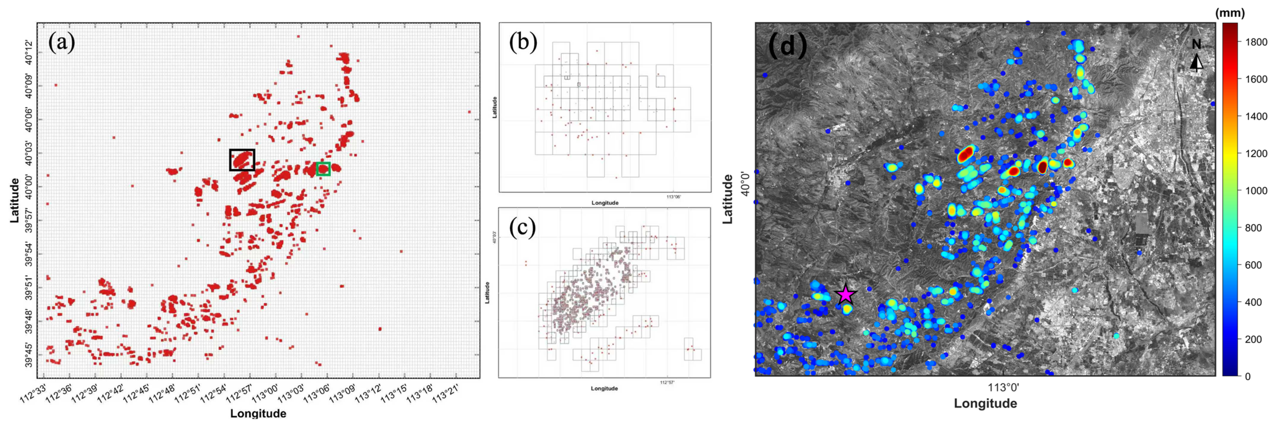
To quantitatively evaluate the ability of different forecasting algorithms to reconstruct the spatial evolution of subsidence during the extrapolation period, the observed InSAR cumulative subsidence field at the 15-step horizon (corresponding to day 180 of the blind forecasting period) was used as a common spatial reference for validation (Figure 4d). Following the spatially stratified heterogeneous sampling strategy described in Section 3.2.1, coherent points with deformation rates greater than −30 mm/year were first excluded to remove stable areas with negligible deformation. The remaining coherent points were then stratified into four deformation-rate intervals (−60 to −30 mm/year, −110 to −60 mm/year, −180 to −110 mm/year, and < −180 mm/year) and assigned to spatial grids with resolutions of 0.005°, 0.002°, 0.001°, and 0.0003°, respectively. These sizes (approx. 500 m, 200 m, 100 m, and 30 m) scale inversely with deformation severity. The 0.0003° grid matches Sentinel-1’s native 30 m resolution to preserve extreme subsidence features, while larger grids filter out redundant peripheral data. This balance prevents the smoothing of peak values in the core and avoids excessive computational burden in the periphery. Figure 4a–c display the corresponding results and two examples of the spatially stratified heterogeneous sampling strategy. Within each grid cell, the coherent point exhibiting the largest deformation rate was selected as the representative sample. This procedure yielded 5894 high-coherence time-series modeling points (Figure 4a) that effectively preserved both the overall deformation pattern and the characteristics of severe subsidence zones.
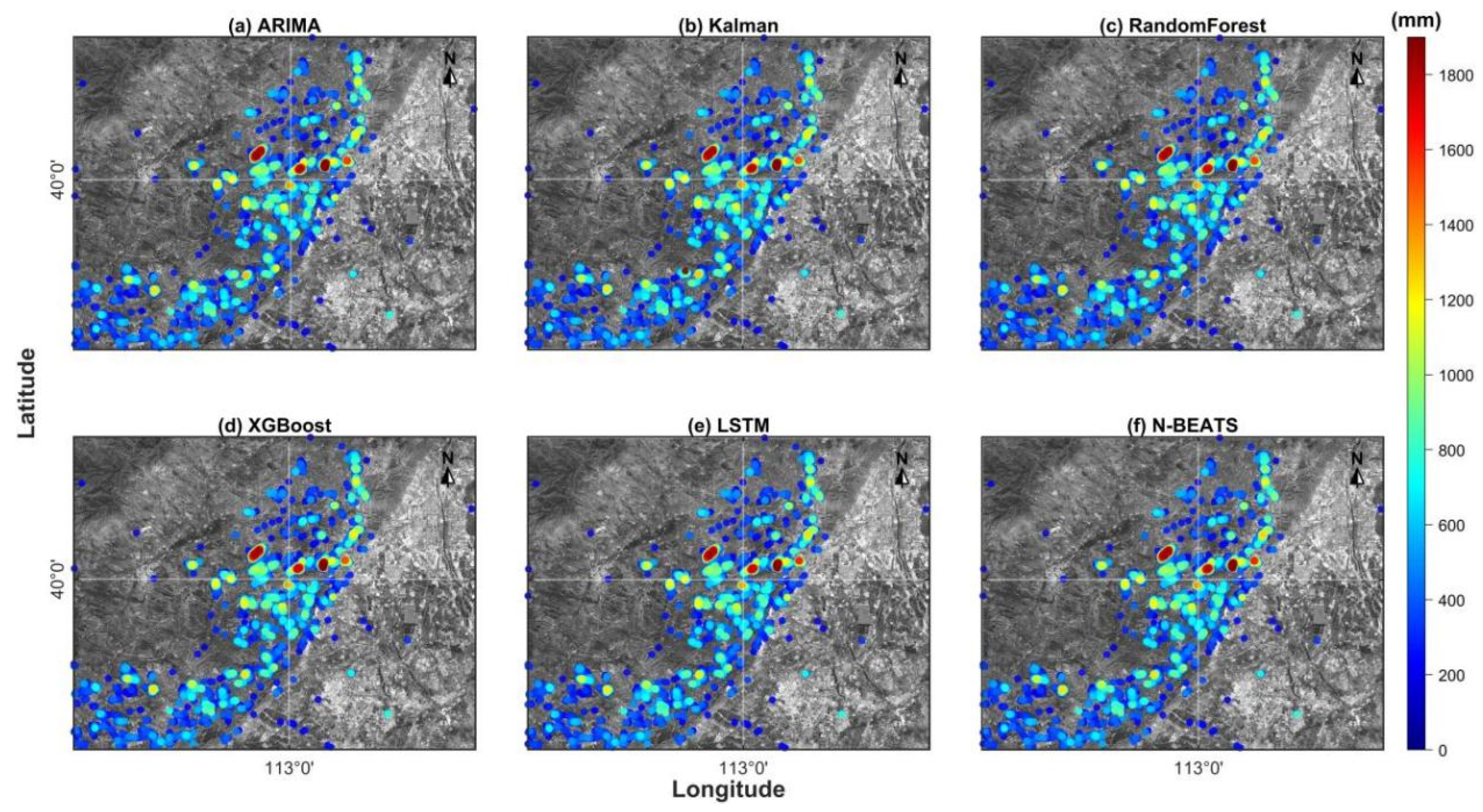
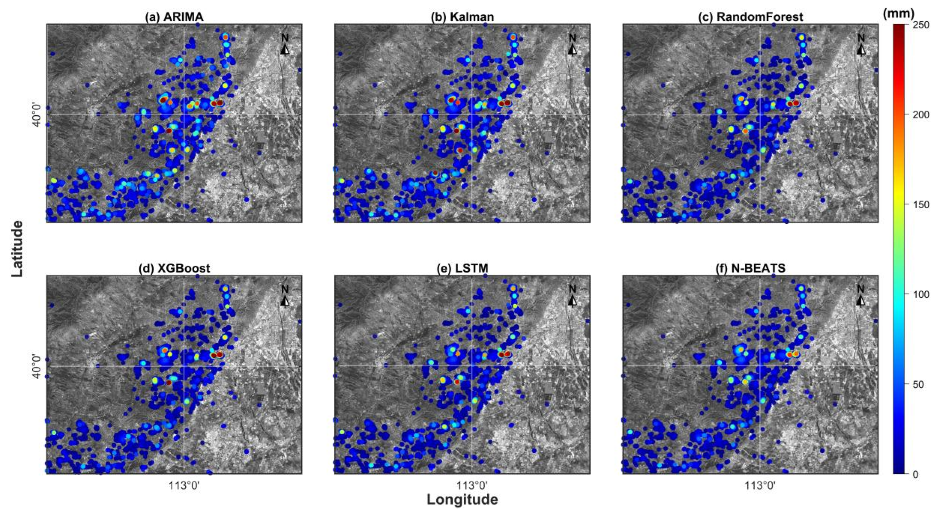
Based on the multi-step forecasting framework described in Section 3.2.2, Figure 5 presents the predicted spatial subsidence fields generated by the six models at the end of the blind forecasting period. At the regional scale, both recursive forecasting approaches and MIMO strategies successfully captured the overall geometry of the major subsidence basins, indicating their ability to reproduce the first-order spatial pattern of mining-induced deformation.
Due to the limited visual discriminability in raster-based displays, multiple modeling points in Figure 5 overlap, making their differences difficult to directly discern. To address this limitation, the observed InSAR cumulative subsidence field in Figure 4d was compared on a point-by-point basis with the corresponding model predictions (Figure 5), and a global absolute residual map for the end of the blind forecasting period was generated (Figure 6). In this residual representation, values closer to zero (blue tones) indicate higher agreement between predicted and observed subsidence.
From the spatial distribution of residuals, traditional time-series models (ARIMA and Kalman), as well as conventional machine learning and deep learning approaches (RF, XGBoost, and LSTM), exhibit pronounced clusters of high residuals (red and yellow patches) in the central subsidence basin, where deformation is most intense. This indicates that these models suffer from varying degrees of error accumulation during long-term extrapolation in highly nonlinear deformation zones. In contrast, the N-BEATS model proposed in this study (Figure 6f) shows the weakest residual patterns across all 5894 sampled points, with residuals predominantly characterized by low-magnitude blue tones. This suggests a substantially improved consistency between predicted and observed subsidence fields. The superior spatial extrapolation performance is attributed to its MIMO forecasting architecture, which reduces temporal error propagation in long-horizon prediction. A more detailed quantitative evaluation of multi-step forecasting accuracy for all models is provided in Table 2.

4.3. Evolution of Ecological Quality and Cross-Lagged Spatial Patterns in Mining Areas

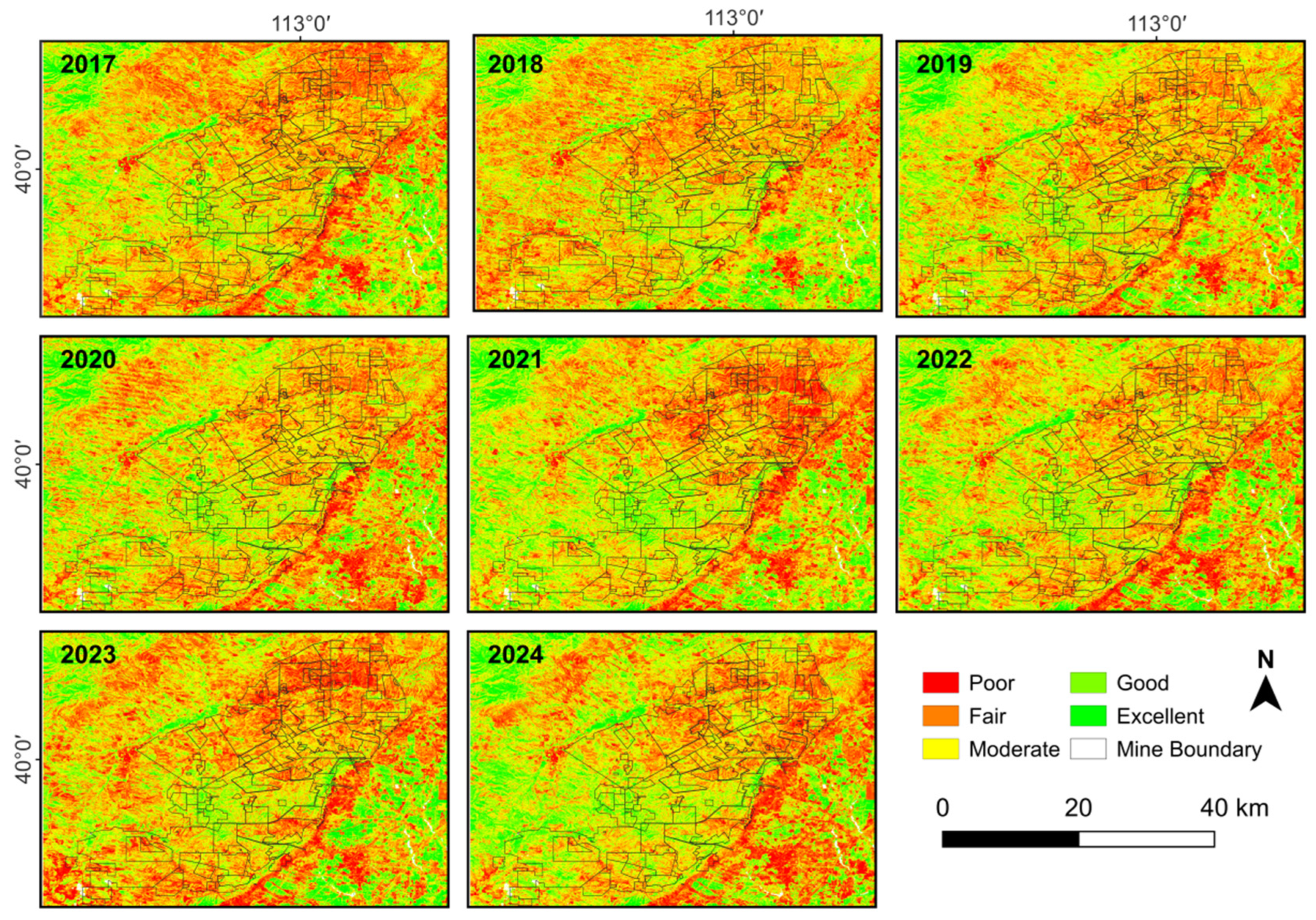
To investigate the disturbance effects of surface deformation on the ecological environment, this study inverted the RSEI of the study area from 2017 to 2024. This inversion was based on Landsat time-series imagery and the methodology detailed in Section 3.3.1. Figure 7 illustrates the spatial distribution pattern of the multi-year average RSEI across the study area. This map is partitioned into five intervals with a spacing of 0.2 to demonstrate variations in ecological quality. Generally, the Datong mining area exhibits a fundamentally fragile ecological baseline, primarily because it is situated within a semi-arid loess-covered region. In peripheral mountainous regions unaffected by mining disturbances, RSEI values remain relatively stable. Conversely, intense mining zones, such as Yanzishan and Majiliang, and their vicinities exhibit a pronounced clustering of low RSEI values. Spatially, this pattern highly coincides with cumulative surface deformation funnels. This intuitively reflects the destructive impact of underground mining on surface vegetation and the ecological soil-water environment.
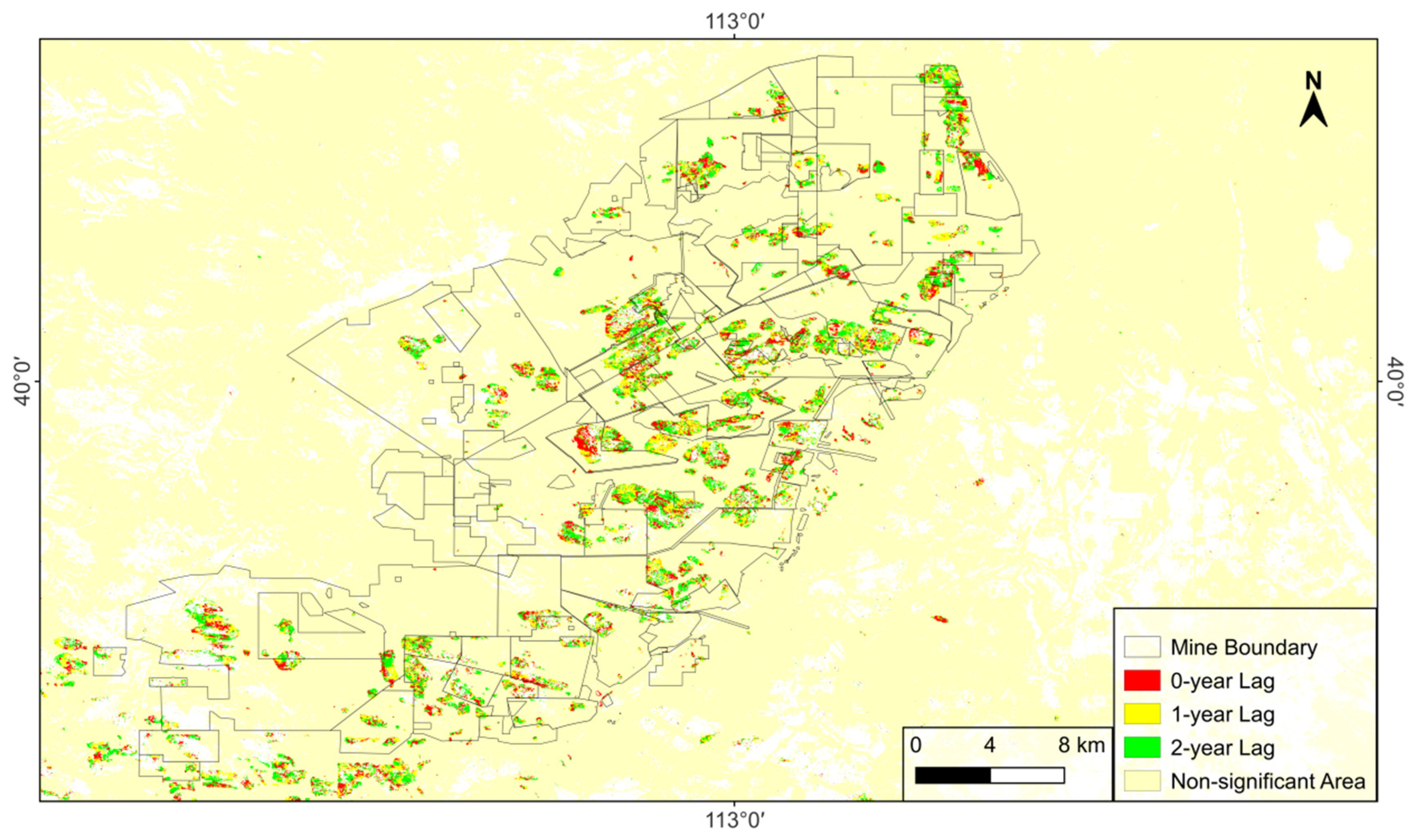
Furthermore, a pixel-scale cross-lagged analysis (detailed in Section 3.3.2) was conducted. This quantitatively extracted the temporal lag of ecological degradation in response to surface deformation within mining-disturbed areas. The corresponding spatial distribution pattern is depicted in Figure 8. A vast light-yellow background, accounting for 95.17% of the total area, represents stable regions without significant mining disturbances (Non-significant Area). However, pixel clusters exhibiting significant ecological-deformation coupled responses (comprising red, yellow, and green patches, totaling 4.83%) are highly aggregated. These patches are precisely nested within and adjacent to the primary active working faces (indicated by black polygonal boundaries). This intuitively confirms the mining-dominated nature of ecological degradation in this region. Spatially, the ecological lag effect exhibits a highly typical “center-edge” concentric heterogeneous differentiation pattern. Specifically, concurrent response areas with no temporal lag (0-year Lag, red patches, 1.37% of the total area) display intense spatial clustering. They predominantly erupt as massive clusters at the geometric centers of high-intensity working faces or deformation extremum zones, reflecting instantaneous ecological damage induced by severe collapse. In contrast, short-term lag areas with temporal buffers (1-year Lag, yellow patches, 1.60%) and long-term lag areas (2-year Lag, green patches, 1.86%) exhibit distinct annular or scattered distributions. These are widely enveloped around the periphery of the red core zones. Alternatively, they are independently distributed at the basin edges where deformation gradients are relatively gentle, thereby constituting an ecological buffer zone for the mining area’s deformation evolution.

5. Discussion

5.1. Validation of InSAR Monitoring Accuracy and Evolution Analysis of Typical Subsidence Zones

5.1.1. Validation of InSAR Monitoring Accuracy

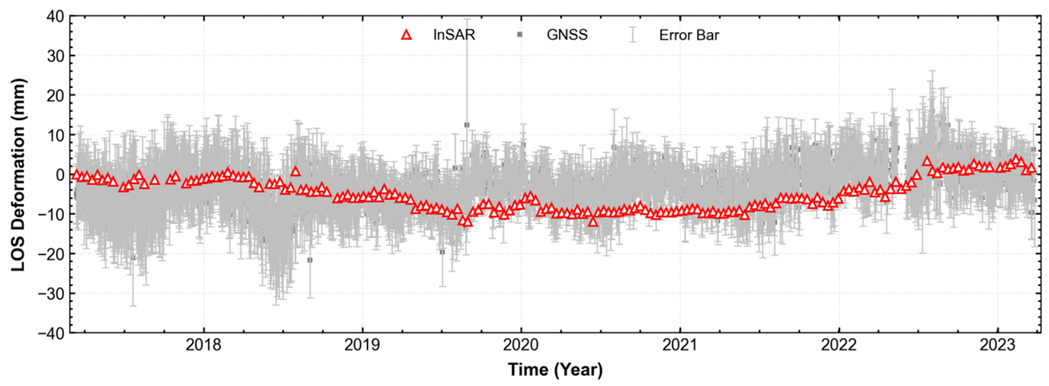
To ensure the reliability of the surface time-series deformation field inverted in Section 4.1, this study conducted cross-validation on the SBAS-InSAR results. This validation utilized measured three-dimensional data from the continuous GNSS station, SXDT, located within the study area (marked in Figure 1 with a purple star). Initially, based on Formula (9) established in Section 3.4.1 of this study, the three-dimensional GNSS displacement components were projected into the radar LOS direction via geometric conversion. This rigorous procedure successfully facilitated a point-to-point time-series comparison (Figure 9).
Examining the time-series comparative trajectories reveals a strong consistency between the continuous GNSS displacement curve and the discrete SBAS-InSAR scatter points. This alignment is particularly evident regarding the macroscopic trend of long-term nonlinear subsidence. Quantitative statistical results indicate that the STD of the difference between the InSAR and GNSS monitoring sequences is 5.58 mm, while the RMSE is 8.79 mm. This level of accuracy demonstrates the reliability of the long-term subsidence monitoring results extracted in this study. It effectively mitigates uncertainty errors directly at the data source. Consequently, it establishes a robust, high-precision foundation for subsequently constructing unbiased datasets and evaluating the multi-step forward blind-test performance of the six mainstream models. Relying on a single GNSS station, however, is inherently limited in spatial representation. Future studies will incorporate broader external measurement data, such as, leveling data, to further evaluate spatial accuracy, when such data becomes available.

5.1.2. Evolution Analysis of Typical Subsidence Zones

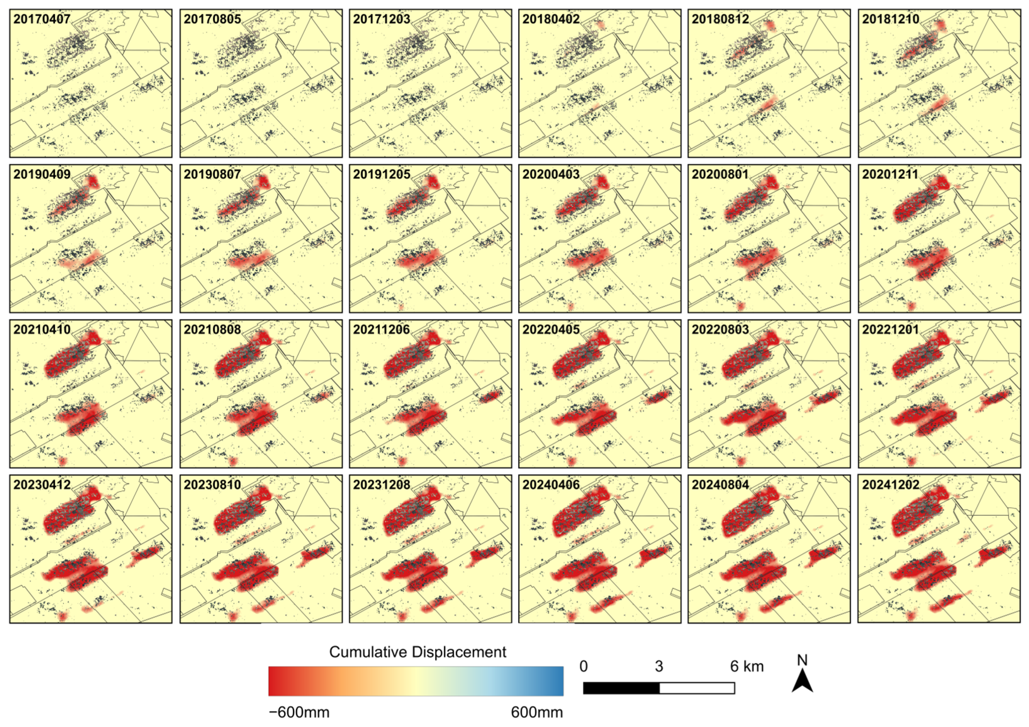
To reveal the spatiotemporal evolution of mining-induced deformation, the Yanzishan-Majiliang mining area was selected as a representative case study (Figure 10). From 2017 to 2018, subsidence was restricted to individual working faces, forming isolated elliptical troughs. Continued multi-seam mining and goaf reactivation subsequently promoted upward deformation propagation and basin expansion. During 2019–2021, overlapping deformation boundaries between adjacent panels led to stress superposition and destabilization of previously stable inter-panel areas. By 2022–2024, the deformation zones had coalesced into a large continuous subsidence basin, with cumulative settlement exceeding −1500 mm and locally reaching −2000 mm. The evolution pattern is strongly nonlinear and spatially heterogeneous, with sustained subsidence in the basin center and abrupt deformation jumps associated with mining advancement and localized collapses.
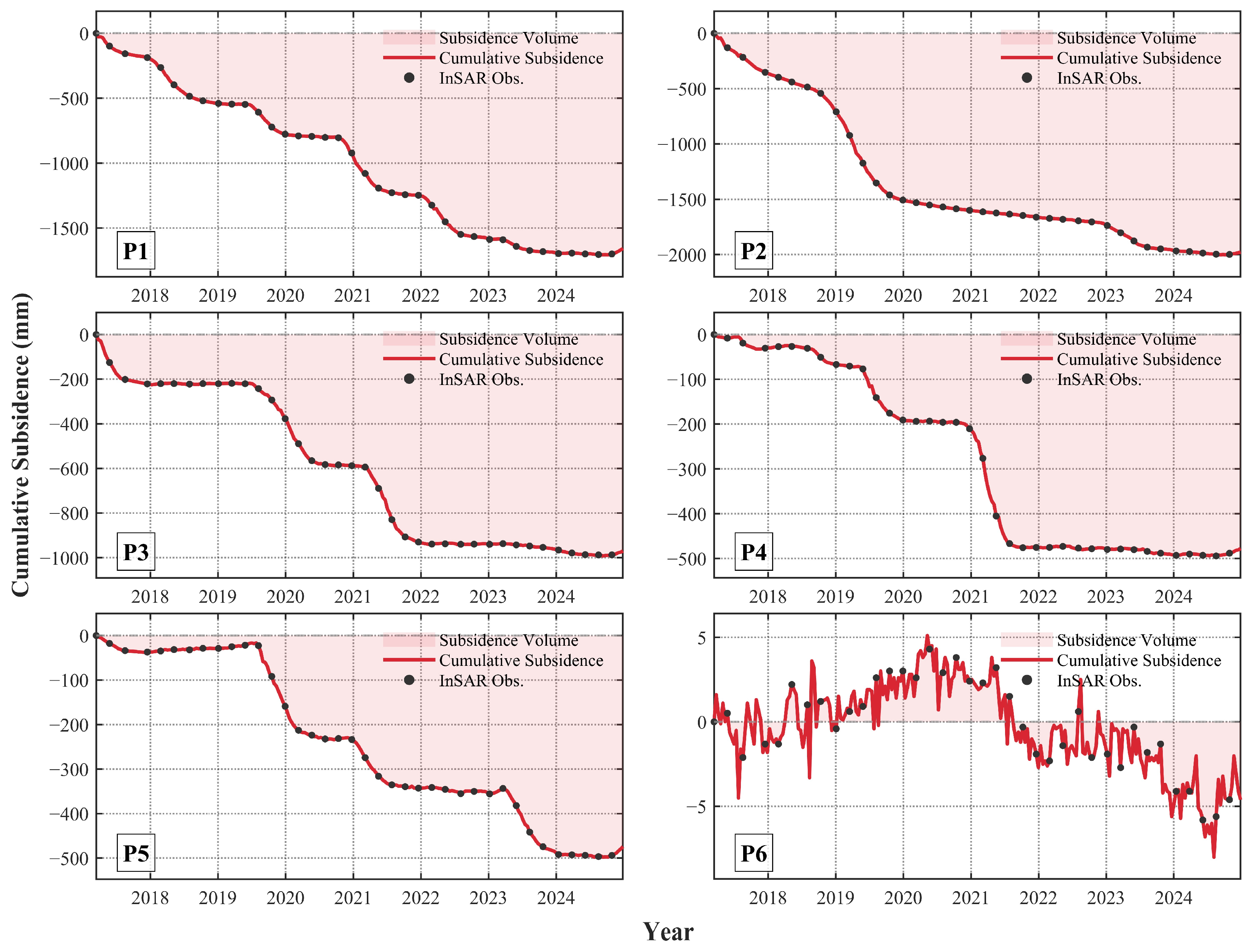
To further examine local nonlinear deformation dynamics, six representative points (P1–P6, marked in Figure 3) were selected for time-series analysis (Figure 11). Distinct deformation behaviors are observed across the study area. P1 and P2, located in the subsidence center, exhibit sustained nonlinear settlement, reaching nearly −1700 mm and −2000 mm, respectively. P3–P5, situated within the transition zone, show pronounced stepwise subsidence, with abrupt deformation episodes corresponding to mining progression and subsequent stabilization. In contrast, P6 remains stable around 0 mm throughout the observation period, serving as a background reference point and further validating the reliability of the SBAS-InSAR results.

5.2. Prediction Accuracy Assessment and Time-Series Evolution Analysis of Characteristic Points

5.2.1. Prediction Accuracy Assessment

The RMSE, MAE, and sMAPE metrics are used for prediction accuracy assessment of 5894 sampled points. The evaluation covers multiple prediction steps (3, 6, 9, 12, and 15 steps; Table 2). As the horizon extends from 3 steps (Day 36) to 15 steps (Day 180), all model errors monotonically increase. Within the 3-step short horizon, the RMSE for all models remains under 7 mm. Here, LSTM (RMSE: 5.78 mm) and RF (MAE: 3.55 mm, sMAPE: 0.58%) perform optimally. However, beyond the 6-step (Day 72) threshold, traditional machine learning errors surge, while N-BEATS consistently outperforms them. At the extreme 15-step horizon, the RMSE of ARIMA and Kalman severely diverges to 26.55 mm and 45.70 mm, respectively. In contrast, N-BEATS stably suppresses the RMSE to 17.98 mm. This confirms that its global mapping strategy effectively blocks cascading error transmission. Ultimately, it demonstrates robust generalization in long-horizon forecasting.
To verify whether the observed error reductions are statistically meaningful, 95% confidence intervals (CIs) and Diebold-Mariano (DM) tests are evaluated (Table 3). Across all forecasting horizons, the CIs reveal that N-BEATS consistently maintains a narrower and lower error bound. For example, within the 3-step short horizon, the N-BEATS CI is [6.65, 7.40], outperforming strong baselines like LSTM ([7.25, 8.08]). Furthermore, the DM test decisively confirms this superiority. Except for XGBoost at the 12-step horizon ( ρ  < 0.05), all other baseline comparisons yield  ρ -values less than 0.01 across all 15 steps. This rejects the null hypothesis, proving that the long-horizon forecasting improvements of N-BEATS are statistically significant rather than artifacts of random noise.
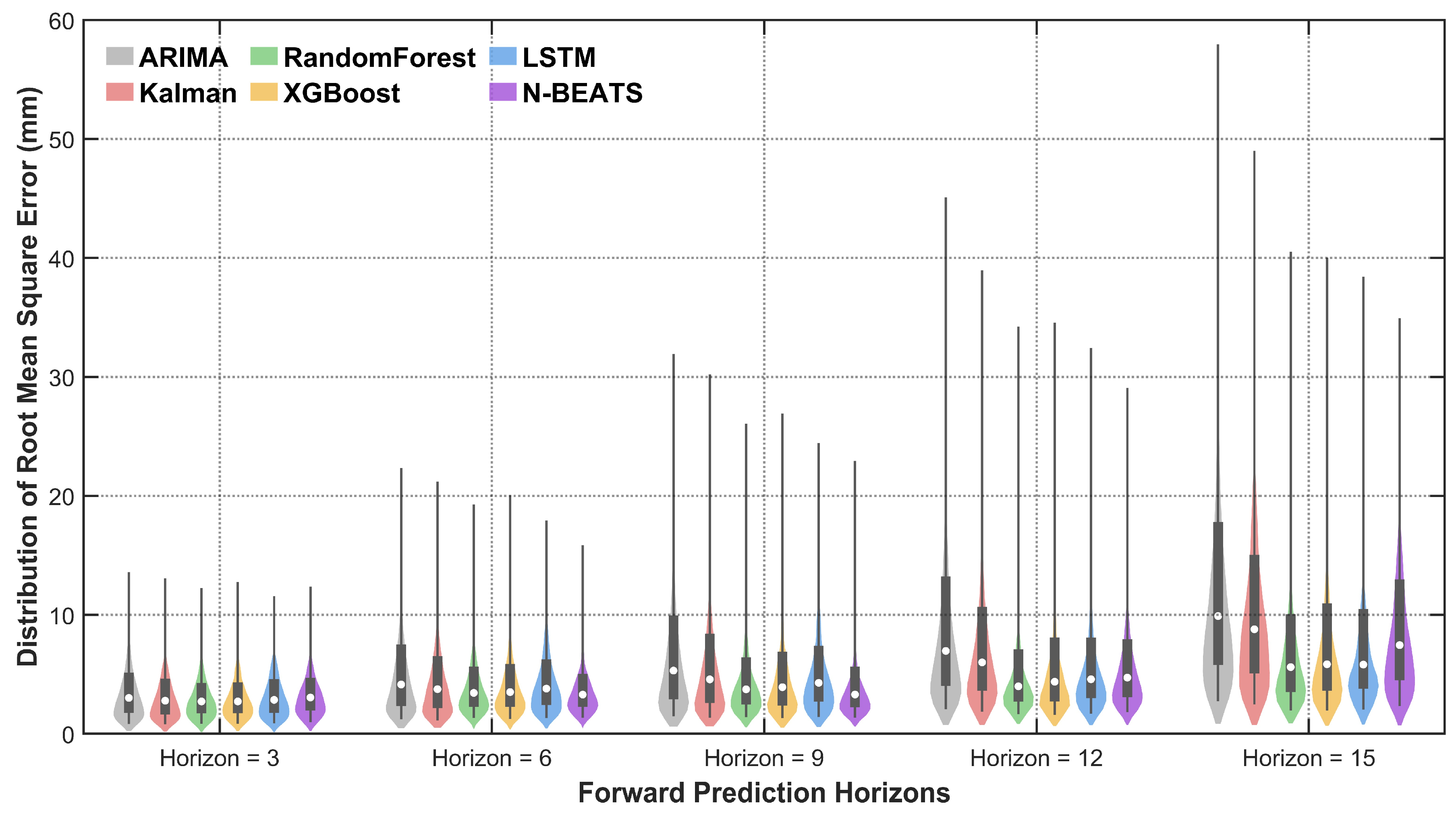
Figure 12 further illustrates the probability distributions of RMSE values for the 5894 smapled points under different forecasting horizons.,. Under the short-term horizon (h = 3), all models exhibit “bottom-heavy” features. Their medians remain exceptionally low (5–7 mm) without obvious divergence. As prediction steps extend (h = 6 to 15), the error centers of traditional recursive models (Kalman, ARIMA) shift upward rapidly. By h = 15, they display severe wide-amplitude divergence. Conventional machine learning and LSTM suppress this central rise. However, they generate pronounced probability long tails within the 20–40 mm high-error zone. In contrast, N-BEATS maintains the most compact morphology across all steps. At the extreme h = 15 limit, its primary trunk retains a “regular teardrop” high-density clustering near the baseline. This objectively demonstrates that N-BEATS effectively suppresses cumulative errors within a low threshold. Ultimately, it globally controls extreme outlier divergence phenomena.

5.2.2. Time-Series Evolution Analysis of Characteristic Points

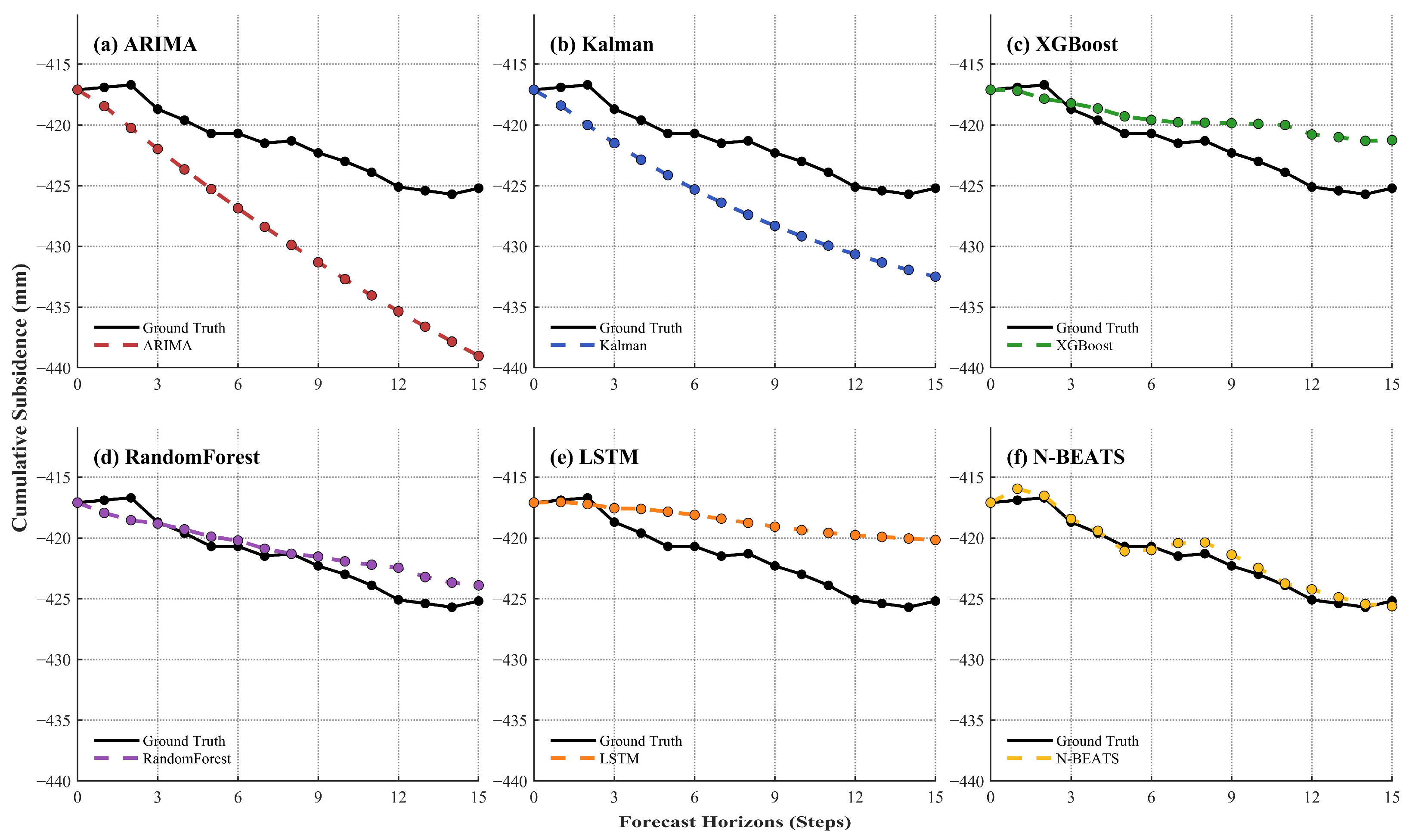
To intuitively reveal the dynamic fitting details and tracking capabilities of various models at specific spatial locations, this section extracts a representative subsidence point. This point is located within the study area and is indicated by a magenta star in Figure 4. Its time-series prediction curves within the 15-step (180-day span) forward extrapolation horizon are independently decoupled and compared. The specific evolutionary trajectory is illustrated in Figure 13.
Observing the single-point, multi-model evolutionary process in Figure 13, the authentic surface deformation (Ground Truth, solid black line) of this characteristic point is evident. It exhibits a continuous nonlinear subsidence feature throughout the 15-step observation period. Confronted with this continuous deformation process, the fitting morphologies of the respective models exhibit significant discrepancies. Traditional models, namely ARIMA (Figure 13a) and the Kalman (Figure 13b), maintained a downward trend. However, their prediction curves significantly deviated and positioned themselves above the true trajectory. This underestimates the actual subsidence magnitude, thereby exposing their systematic bias during long-sequence extrapolation. Conventional machine learning models, XGBoost (Figure 13c) and RF (Figure 13d), demonstrated satisfactory fitting during the initial prediction stages. Nevertheless, during the long-step accumulation phase (Steps 9 to 15), both prediction curves exhibited varying degrees of “underfitting.” This reflects a fundamental vulnerability of tree-based algorithms. When addressing continuous long-time-series trend extrapolation, they are prone to producing smooth attenuation at the tail. The deep learning LSTM model (Figure 13e) achieved commendable fitting during the early prediction phase (prior to Step 3). However, in subsequent stages (Steps 3 to 15), it significantly deviated from the true trajectory. Consequently, it failed to effectively track the accelerated subsidence occurring in the middle and late stages. In stark contrast, the N-BEATS model (Figure 13f) demonstrated the most precise fitting performance within this typical deformation period. Throughout the entire 15-step evolutionary cycle, the predicted scatter points and curve (dashed yellow line) of N-BEATS closely aligned with the actual subsidence trajectory. This microscopic visual comparison objectively confirms a critical capability. The N-BEATS architecture can acutely capture and reconstruct the true dynamic laws of subsidence locations. Furthermore, it maintains high tracking accuracy during long-term time-series extrapolation.

5.3. Driving Mechanisms of Ecological Response Lag

Section 4.3 presents cross-lagged results indicating that mining-induced ecological degradation in the Datong coal mining area exhibits a pronounced core–periphery pattern in temporal lag heterogeneity. Areas showing significant coupled responses (4.83% of the study region) are primarily concentrated along major working faces and their surrounding zones. This spatiotemporal mismatch is not a random artifact but is governed by differentiated surface damage and hydrological disturbance mechanisms across spatial gradients [1,2].
In the central subsidence zone, ecological responses occur without detectable temporal lag (Lag 0, accounting for 1.37%). Geomechanical studies have shown that rapid coal extraction is accompanied by high-gradient, stepwise subsidence and intensive surface fracture development [4]. Such discontinuous deformation directly induces mechanical damage to shallow root systems and accelerates rapid soil moisture loss. The deformation intensity exceeds the self-recovery threshold of vegetation, leading to abrupt spectral degradation and explaining the synchronous behavior between deformation and RSEI decline in the core area.
In contrast, the peripheral buffer zones of the basin generally exhibit delayed ecological responses of 1–2 years. In these areas, surface deformation is characterized by gentle and continuous bending subsidence. Based on the mechanism established in the literature [15], we hypothesize that this lag is driven by groundwater table decline and progressive soil moisture depletion. Ecohydrological studies further indicate that deep conductive fracture networks induced by mining can impose long-term water stress on root systems [16,17]. However, vegetation in semi-arid environments exhibits a degree of physiological drought resilience, enabling a delayed response over periods ranging from months to years. During the early stage of groundwater decline, vegetation can temporarily maintain canopy greenness. Only when moisture deficits exceed physiological tolerance does chlorophyll degradation become pronounced, resulting in a significant decrease in RSEI after a lag of 1–2 years. This process reflects an implicit ecological degradation mechanism driven by the cascade of groundwater loss–soil moisture transport–vegetation physiological response. Although using annual growing-season data minimizes seasonal phenological noise and cloud interference, the 8-year sample size is relatively small and may be sensitive to outliers. Future studies should utilize monthly or seasonal data to increase the sample size and provide more statistically robust lag estimates once such data become available. Furthermore, a notable limitation of this study is that the proposed framework was validated on a single mining area. While the Datong Coalfield is highly representative, future research should test the generalizability of these global models across multiple distinct mining basins.

6. Conclusions

An integrated framework was developed to couple long-horizon deformation forecasting with ecological lag-effect analysis. Using deformation time series derived from 231 Sentinel-1A images, 5894 representative points were selected to reduce spatial sampling bias. Six forecasting models were then evaluated using a reconstructed sliding-window strategy. Ecological dynamics were characterized using the RSEI, and cross-lagged analysis was applied to quantify the spatiotemporal relationships between ground deformation and ecological change. The primary conclusions are as follows:
(1)
Ground deformation was highly heterogeneous across the mining area. While deformation rates in the peripheral zones generally remained below −30 mm/year, the central subsidence basin was characterized by abrupt nonlinear collapse and rapid ground settlement. Peak deformation rates reached −276.75 mm/year, and cumulative subsidence exceeded −2000 mm in the most intensively mined sectors.
(2)
The comparison of six forecasting models showed that controlling error propagation is essential for maintaining predictive accuracy during long-term forecasting of abrupt subsidence events. Within the first three forecasting steps, all models maintained high predictive accuracy, with RMSE values below 7 mm. When the forecasting horizon was extended to 15 steps, conventional recursive models exhibited severe error divergence, with the Kalman model’s RMSE increasing sharply to 45.70 mm. In contrast, N-BEATS effectively mitigated temporal error propagation by employing a MIMO strategy, which prevents stepwise error accumulation, and maintained a stable global RMSE of 17.98 mm at the 15-step horizon, demonstrating excellent robustness against cumulative error growth in long-term prediction.
(3)
Cross-lagged analysis reveals a clear core-periphery pattern in the temporal evolution of mining-induced ecological degradation. In the central subsidence zone, ecological deterioration occurred immediately following surface disruption, with no observable time lag (Lag 0, 1.37%). By contrast, peripheral areas exhibited delayed responses of 1–2 years, accounting for 1.60% (Lag 1) and 1.86% (Lag 2), respectively. This delayed degradation is likely controlled by the balance between vegetation resilience and progressive soil moisture depletion.
Future research will aim to expand this integrated framework to multiple distinct mining basins to further verify its generalizability.

Author Contributions

Conceptualization, L.Z. and L.D.; methodology, L.Z.; software, L.Z.; validation, L.Z. and S.Z.; formal analysis, L.Z.; investigation, L.Z. and L.D.; resources, L.D.; data curation, L.Z. and L.D.; writing—original draft preparation, L.Z.; writing—review and editing, L.Z., L.D. and S.Z.; visualization, L.Z.; supervision, L.D.; project administration, L.D.; funding acquisition, L.D. All authors have read and agreed to the published version of the manuscript.

Funding

This research was funded by the Engineering Technology Innovation Center for Ecological Protection and Restoration in the Middle Yellow River, Ministry of Natural Resources (No. 2025069), the Key Laboratory of Ionic Rare Earth Resources and Environment, Ministry of Natural Resources of the People’s Republic of China (No. 2024IRERE403), the Natural Science Foundation of Shanxi Province (Grant No. 202403021211007), and the National Natural Science Foundation of China (42271432).

Data Availability Statement

Sentinel-1A SAR images are available through the Alaska Satellite Facility Vertex website (ASF; https://search.asf.alaska.edu/; accessed on 15 March 2026); Landsat 8 and 9 OLI/TIRS images are available through the U.S. Geological Survey website (USGS; https://earthexplorer.usgs.gov/; accessed on 20 March 2026); Sentinel-1 Precise Orbit Determination (POD) auxiliary data (POEORB) are available at the ESA STEP auxiliary data server (http://step.esa.int/auxdata/orbits/Sentinel-1/POEORB/S1A/; accessed on 15 March 2026); SRTM Digital Elevation Model (DEM) data are available at the U.S. Geological Survey website (USGS; http://earthexplorer.usgs.gov/; accessed on 15 March 2026); GNSS monitoring data are available at the Earthquake Data Service Center (EQDSC; https://data.earthquake.cn/index.html; accessed on 15 March 2026); administrative boundaries are available at the Resource and Environment Science and Data Center (RESDC; https://www.resdc.cn/; accessed on 15 March 2026).

Conflicts of Interest

The authors declare no conflicts of interest.

References

  1. Bian, Z.; Inyang, H.I.; Daniels, J.L.; Otto, F.; Struthers, S. Environmental issues from coal mining and their solutions. Min. Sci. Technol. (China) 2010, 20, 215–223. [Google Scholar] [CrossRef] [Scilit]
  2. Hou, H.; Ding, Z.; Zhang, S.; Guo, S.; Yang, Y.; Chen, Z.; Mi, J.; Wang, X. Spatial estimate of ecological and environmental damage in an underground coal mining area on the Loess Plateau: Implications for planning restoration interventions. J. Clean. Prod. 2021, 287, 125061. [Google Scholar] [CrossRef] [Scilit]
  3. Guo, W.; Zhao, G.; Bai, E.; Guo, M.; Wang, Y. Effect of overburden bending deformation and alluvium mechanical parameters on surface subsidence due to longwall mining. Bull. Eng. Geol. Environ. 2021, 80, 2751–2764. [Google Scholar] [CrossRef] [Scilit]
  4. Ju, J.; Xu, J. Surface stepped subsidence related to top-coal caving longwall mining of extremely thick coal seam under shallow cover. Int. J. Rock Mech. Min. Sci. 2015, 78, 27–35. [Google Scholar] [CrossRef] [Scilit]
  5. Zhang, B.; Chang, L.; Stein, A. Spatio-temporal linking of multiple SAR satellite data from medium and high resolution Radarsat-2 images. ISPRS J. Photogramm. Remote Sens. 2021, 176, 222–236. [Google Scholar] [CrossRef] [Scilit]
  6. Zhang, B.; Chang, L.; Stein, A. A model-backfeed deformation estimation method for revealing 20-year surface dynamics of the Groningen gas field using multi-platform SAR imagery. Int. J. Appl. Earth Obs. Geoinf. 2022, 111, 102847. [Google Scholar] [CrossRef] [Scilit]
  7. Zhang, B.; Chang, L.; Wang, Z.; Wang, L.; Ye, Q.; Stein, A. Multi-decadal Dutch coastal dynamic mapping with multi-source remote sensing imagery. Int. J. Appl. Earth Obs. Geoinf. 2025, 138, 104452. [Google Scholar] [CrossRef] [Scilit]
  8. Shu, C.; Meng, Z.; Yang, Y.; Wang, Y.; Liu, S.; Zhang, X.; Zhang, Y. Deep learning-based InSAR time-series deformation prediction in coal mine areas. Geo-Spat. Inf. Sci. 2025, 28, 2119–2141. [Google Scholar] [CrossRef] [Scilit]
  9. Ribeiro, R.P.; Moniz, N. Imbalanced regression and extreme value prediction. Mach. Learn. 2020, 109, 1803–1835. [Google Scholar] [CrossRef] [Scilit]
  10. Yang, Y.; Zha, K.; Chen, Y.; Wang, H.; Katabi, D. Delving into deep imbalanced regression. In Proceedings of the 38th International Conference on Machine Learning, Virtual, 18–24 July 2021; pp. 11842–11851. [Google Scholar]
  11. Taieb, S.B.; Bontempi, G.; Atiya, A.F.; Sorjamaa, A. A review and comparison of strategies for multi-step ahead time series forecasting based on the NN5 forecasting competition. Expert Syst. Appl. 2012, 39, 7067–7083. [Google Scholar] [CrossRef] [Scilit]
  12. Wen, R.; Torkkola, K.; Narayanaswamy, B.; Madeka, D. A multi-horizon quantile recurrent forecaster. arXiv 2017, arXiv:1711.11053. [Google Scholar]
  13. Zhang, L.; Su, Q.; Zhang, B.; Xue, H.; Zuo, Z.; Li, Y.; Zheng, H. Integrating Surface Deformation and Ecological Indicators for Mining Environment Assessment: A Novel MDECI Approach. Remote Sens. 2026, 18, 1272. [Google Scholar] [CrossRef] [Scilit]
  14. Chen, Y.; Suo, Z.; Lu, H.; Cheng, H.; Li, Q. Active–passive remote sensing evaluation of ecological environment quality in Juye mining area, China. Remote Sens. 2023, 15, 5750. [Google Scholar] [CrossRef] [Scilit]
  15. Xiao, W.; Zhang, W.; Ye, Y.; Lv, X.; Yang, W. Is underground coal mining causing land degradation and significantly damaging ecosystems in semi-arid areas? A study from an Ecological Capital perspective. Land Degrad. Dev. 2020, 31, 1969–1989. [Google Scholar] [CrossRef] [Scilit]
  16. Vicente-Serrano, S.M.; Gouveia, C.; Camarero, J.J.; Beguería, S.; Trigo, R.; López-Moreno, J.I.; Azorín-Molina, C.; Pasho, E.; Lorenzo-Lacruz, J.; Revuelto, J.; et al. Response of vegetation to drought time-scales across global land biomes. Proc. Natl. Acad. Sci. USA 2013, 110, 52–57. [Google Scholar] [CrossRef] [Scilit] [PubMed]
  17. Wu, D.; Zhao, X.; Liang, S.; Zhou, T.; Huang, K.; Tang, B.; Zhao, W. Time-lag effects of global vegetation responses to climate change. Glob. Change Biol. 2015, 21, 3520–3531. [Google Scholar] [CrossRef] [Scilit] [PubMed]
  18. Salmi, E.F.; Nazem, M.; Karakus, M. The effect of rock mass gradual deterioration on the mechanism of post-mining subsidence over shallow abandoned coal mines. Int. J. Rock Mech. Min. Sci. 2017, 91, 59–71. [Google Scholar] [CrossRef] [Scilit]
  19. Liu, S.; Li, W.; Qiao, W.; Wang, Y.; Hu, Y.; Wang, Z. Effect of natural conditions and mining activities on vegetation variations in arid and semiarid mining regions. Ecol. Indic. 2019, 103, 331–345. [Google Scholar] [CrossRef] [Scilit]
  20. Sui, W.; Hang, Y.; Ma, L.; Zhou, Y.; Long, G.; Wei, L. Interactions of overburden failure zones due to multiple-seam mining using longwall caving. Bull. Eng. Geol. Environ. 2015, 74, 1019–1035. [Google Scholar] [CrossRef] [Scilit]
  21. Ghabraie, B.; Ren, G.; Barbato, J.; Smith, J.V. A predictive methodology for multi-seam mining induced subsidence. Int. J. Rock Mech. Min. Sci. 2017, 93, 280–294. [Google Scholar] [CrossRef] [Scilit]
  22. Torres, R.; Snoeij, P.; Geudtner, D.; Bibby, D.; Davidson, M.; Attema, E.; Potin, P.; Rommen, B.; Floury, N.; Brown, M.; et al. GMES Sentinel-1 mission. Remote Sens. Environ. 2012, 120, 9–24. [Google Scholar] [CrossRef] [Scilit]
  23. Fernández, M.; Peter, H.; Arnold, D.; Duan, B.; Simons, W.; Wermuth, M.; Hackel, S.; Fernández, J.; Jäggi, A.; Hugentobler, U.; et al. Copernicus Sentinel–1 POD reprocessing campaign. Adv. Space Res. 2022, 70, 249–267. [Google Scholar] [CrossRef] [Scilit]
  24. Farr, T.G.; Rosen, P.A.; Caro, E.; Crippen, R.; Duren, R.; Hensley, S.; Kobrick, M.; Paller, M.; Rodriguez, E.; Roth, L.; et al. The shuttle radar topography mission. Rev. Geophys. 2007, 45, RG2004. [Google Scholar] [CrossRef] [Scilit]
  25. National Earthquake Data Center (NEDC). Available online: https://data.earthquake.cn (accessed on 15 March 2026).
  26. Yu, C.; Li, Z.; Penna, N.T.; Crippa, P. Generic atmospheric correction model for interferometric synthetic aperture radar observations. J. Geophys. Res. Solid Earth 2018, 123, 9202–9222. [Google Scholar] [CrossRef] [Scilit]
  27. Yu, C.; Penna, N.T.; Li, Z. Generation of real-time mode high-resolution water vapor fields from GPS observations. J. Geophys. Res. Atmos. 2017, 122, 2008–2025. [Google Scholar] [CrossRef] [Scilit]
  28. Masek, J.G.; Wulder, M.A.; Markham, B.; Meyn, J.; Hewson, J.; Valle, J.; Murphy, M.; Rengarajan, R.; Vermote, E. Landsat 9: Empowering open science and applications through continuity. Remote Sens. Environ. 2020, 248, 111968. [Google Scholar] [CrossRef] [Scilit]
  29. Gorelick, N.; Hancher, M.; Dixon, M.; Ilyushchenko, S.; Thau, D.; Moore, R. Google Earth Engine: Planetary-scale geospatial analysis for everyone. Remote Sens. Environ. 2017, 202, 18–27. [Google Scholar] [CrossRef] [Scilit]
  30. Berardino, P.; Fornaro, G.; Lanari, R.; Sansosti, E. A new algorithm for surface deformation monitoring based on small baseline differential SAR interferograms. IEEE Trans. Geosci. Remote Sens. 2002, 40, 2375–2383. [Google Scholar] [CrossRef] [Scilit]
  31. Wang, J.F.; Zhang, T.L.; Fu, B.J. A measure of spatial stratified heterogeneity. Ecol. Indic. 2016, 67, 250–256. [Google Scholar] [CrossRef] [Scilit]
  32. Herzen, J.; Lässig, F.; Piazzetta, S.G.; Neuer, T.; Tafti, L.; Raje, S.; Raepsaet, G.; Sproll, M.; Vschinsky, A. Darts: User-friendly modern machine learning for time series. J. Mach. Learn. Res. 2022, 23, 1–6. [Google Scholar]
  33. Box, G.E.P.; Jenkins, G.M.; Reinsel, G.C.; Ljung, G.M. Time Series Analysis: Forecasting and Control, 5th ed.; John Wiley & Sons: Hoboken, NJ, USA, 2015. [Google Scholar]
  34. Kalman, R.E. A new approach to linear filtering and prediction problems. J. Basic Eng. 1960, 82, 35–45. [Google Scholar] [CrossRef] [Scilit]
  35. Breiman, L. Random forests. Mach. Learn. 2001, 45, 5–32. [Google Scholar] [CrossRef] [Scilit]
  36. Chen, T.; Guestrin, C. XGBoost: A scalable tree boosting system. In Proceedings of the 22nd ACM SIGKDD International Conference on Knowledge Discovery and Data Mining, San Francisco, CA, USA, 13–17 August 2016; pp. 785–794. [Google Scholar]
  37. Hochreiter, S.; Schmidhuber, J. Long short-term memory. Neural Comput. 1997, 9, 1735–1780. [Google Scholar] [CrossRef] [Scilit] [PubMed]
  38. Oreshkin, B.N.; Carpov, D.; Chapados, N.; Bengio, Y. N-BEATS: Neural basis expansion analysis for interpretable time series forecasting. In Proceedings of the 8th International Conference on Learning Representations (ICLR), Virtual, 26–30 April 2020. [Google Scholar]
  39. Xu, H.; Wang, Y.; Guan, H.; Shi, T.; Hu, X. Detecting ecological changes with a remote sensing based ecological index (RSEI) produced time series and change vector analysis. Remote Sens. 2019, 11, 2345. [Google Scholar] [CrossRef] [Scilit]
  40. Wright, T.J.; Parsons, B.E.; Lu, Z. Toward mapping surface deformation in three dimensions using InSAR. Geophys. Res. Lett. 2004, 31, L01607. [Google Scholar] [CrossRef] [Scilit]
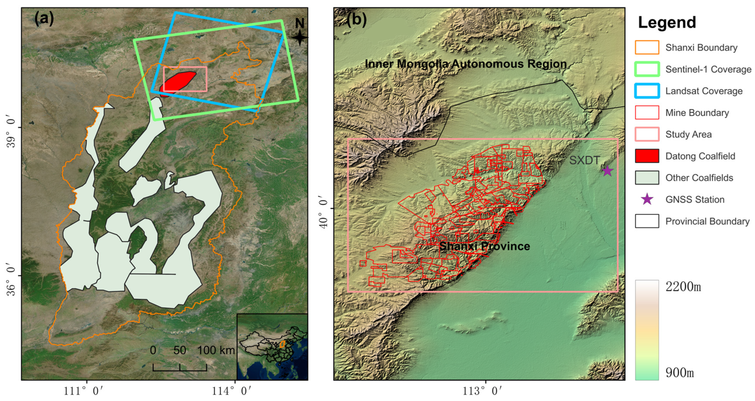
Figure 1. Overview of the study area: (a) Geographical location of the Datong Coalfield in Shanxi Province, China, including the spatial coverage of Sentinel-1 (green rectangle) and Landsat (blue rectangle) data; (b) Topographic map of the study area, showing the boundaries of the mining area and the location of the SXDT GNSS station.
Remotesensing 18 02829 g001
Figure 2. Technical flowchart of the research.
Remotesensing 18 02829 g002
Figure 3. The annual mean surface deformation rate in the Datong coalfield (2017–2024). The black lines indicate the mining area boundaries. The green dots (P1–P6) are analyzed in detail in Section 5.1.2.
Remotesensing 18 02829 g003
Figure 4. (a) Distribution of the 5894 selected high-coherence measurement points after spatially stratified decimation, where the black and green boxes highlight representative regions for demonstrating the grid refinement logic. (b) Detailed multi-scale grid refinement within the green box (severe subsidence region). (c) Detailed multi-scale grid refinement within the black box (moderate subsidence region). (d) Spatial reference of the observed cumulative subsidence field at the 15-step horizon (day 180). The magenta star is analyzed in detail in Section 5.2.2.
Remotesensing 18 02829 g004
Figure 5. Predicted cumulative subsidence fields at the 15-step forecast horizon for: (a) ARIMA, (b) Kalman, (c) RF, (d) XGBoost, (e) LSTM, and (f) N-BEATS.
Remotesensing 18 02829 g005
Figure 6. Absolute prediction residuals at the 15-step forecast horizon for: (a) ARIMA, (b) Kalman, (c) RF, (d) XGBoost, (e) LSTM, and (f) N-BEATS.
Remotesensing 18 02829 g006
Figure 7. Spatial distribution of RSEI in the mining area (2017–2024).
Remotesensing 18 02829 g007
Figure 8. Spatial distribution of the cross-lagged response time between deformation and ecological quality.
Remotesensing 18 02829 g008
Figure 9. Cross-validation between SBAS-InSAR monitoring results and GNSS-measured data.
Remotesensing 18 02829 g009
Figure 10. Spatiotemporal evolution of cumulative surface deformation in the Yanzishan and Majiliang mining areas from 2017 to 2024. The black polygons represent the boundaries of the mining area.
Remotesensing 18 02829 g010
Figure 11. Long-term cumulative subsidence evolution curves for the six typical characteristic points (P1–P6).
Remotesensing 18 02829 g011
Figure 12. Probability density distribution of RMSE for all models under different forward prediction horizons.
Remotesensing 18 02829 g012
Figure 13. Comparison of multi-model time-series prediction fitting curves for a typical characteristic point. The black solid line represents the ground truth, while the colored dashed lines show the predicted values for each model over 15 forward steps. (a) ARIMA; (b) Kalman; (c) XGBoost; (d) RandomForest; (e) LSTM; (f) N-BEATS.
Remotesensing 18 02829 g013
Table 1. Hyperparameter values applied to the selected forecasting models.
ModelOptimal Hyperparameters
ARIMAp = 1, d = 1, q = 1
Kalmandim_x = 2
RFlags = 24, n_estimators = 100, random_state = 42
XGBoostlags = 24, n_estimators = 100, random_state = 42
LSTMinput_chunk_length = 24, output_chunk_length = 1, hidden_dim = 64, n_epochs = 50
N-BEATSinput_chunk_length = 24, output_chunk_length = 15, n_epochs = 50
Table 2. Comprehensive comparison of accuracy metrics for multiple models under different forward prediction steps. The units for RMSE and MAE are mm, and the unit for sMAPE is %.
ModelMetricsh = 3h = 6h = 9h = 12h = 15
ARIMARMSE6.7511.0515.6520.9326.55
MAE4.116.118.1910.6513.7
sMAPE0.690.981.281.622.02
KalmanRMSE6.9612.0718.8128.9845.7
MAE3.815.647.459.5712.28
sMAPE0.660.941.21.491.84
RFRMSE6.029.4612.916.5219.93
MAE3.555.066.247.318.97
sMAPE0.580.790.951.11.32
XGBoostRMSE6.3910.2214.0117.8621.34
MAE3.675.296.647.869.53
sMAPE0.590.8211.171.4
LSTMRMSE5.788.912.0615.5418.91
MAE3.585.136.47.498.97
sMAPE0.60.8211.161.37
N-BEATSRMSE6.128.0111.0214.2617.98
MAE3.894.495.346.849.19
sMAPE0.620.710.841.041.34
Table 3. Comprehensive statistical evaluation of RMSE for multiple models under different forward prediction steps. The unit for 95% CI is mm, and DM ( ρ ) represents the Diebold-Mariano statistic and  ρ -value.
ModelMetricsh = 3h = 6h = 9h = 12h = 15
N-BEATSCI[6.65, 7.40][10.48, 12.13][15.72, 17.73][22.81, 25.35][30.53, 32.78]
ARIMACI[8.57, 9.38][15.84, 17.57][23.47, 25.82][34.23, 37.50][44.36, 48.07]
DM   ( ρ )18.88 (<0.01)20.99 (<0.01)21.63 (<0.01)14.63 (<0.01)12.17 (<0.01)
KalmanCI[8.31, 11.20][15.21, 25.25][22.12, 50.62][31.67, 97.58][39.71, 186.99]
DM   ( ρ )12.29 (<0.01)13.93 (<0.01)11.86 (<0.01)5.84 (<0.01)3.57 (<0.01)
RFCI[7.63, 8.46][13.28, 15.00][18.47, 20.73][25.40, 28.61][30.97, 34.21]
DM   ( ρ )14.96 (<0.01)15.69 (<0.01)9.40 (<0.01)−5.36 (<0.01)−7.28 (<0.01)
XGBoostCI[8.12, 9.04][14.30, 16.26][19.95, 22.62][27.06, 30.76][32.31, 36.03]
DM   ( ρ )15.39 (<0.01)14.73 (<0.01)10.49 (<0.01)−2.43 (<0.05)−5.07 (<0.01)
LSTMCI[7.25, 8.08][12.39, 14.13][17.15, 19.31][24.11, 27.46][29.83, 33.17]
DM   ( ρ )14.99 (<0.01)21.22 (<0.01)13.52 (<0.01)−6.23 (<0.01)−8.67 (<0.01)
Disclaimer/Publisher’s Note: The statements, opinions and data contained in all publications are solely those of the individual author(s) and contributor(s) and not of MDPI and/or the editor(s). MDPI and/or the editor(s) disclaim responsibility for any injury to people or property resulting from any ideas, methods, instructions or products referred to in the content.