A Road-Segment-Based Rockfall Susceptibility Mapping Approach Integrating Physically Informed Slope-Cutting Features and Comparative Machine Learning Models

Highlights

What are the main findings?

• Integrating the physics-informed descriptor $H_{\mathrm{cut}}$ into the vector Road Evaluation Unit (REU) framework resolves coarse raster terrain-smoothing effects, precisely capturing sharp geomechanical gradients induced by technical slope-toe excavations.
• Multi-scenario benchmarking under Leave-One-Road-Corridor-Out Validation (LORCOV) demonstrates that tree-based ensembles maintain high structural resilience against spatial autocorrelation and sampling biases, whereas legacy deep learning models suffer from tabular inductive bias mismatch.

What are the implications of the main findings?

• The proposed REU framework bridges the gap between macro-scale regional geohazard zoning and micro-scale localized slope engineering reinforcement along mountainous transportation corridors.
• Target-tiered threshold analysis directly translates abstract susceptibility indices into actionable intervention mileage, providing concrete decision support for constrained highway maintenance budgets.

Abstract

Rockfall hazards are frequently observed within mountainous road networks. Significant uncertainties regarding the optimal selection of evaluation units and spatial modeling scales are still being identified in this field. A comprehensive comparative framework for rockfall susceptibility mapping is presented in this study, using Wufeng County as the empirical study area. Five evaluation scenarios were constructed to systematically isolate the independent predictive contributions of the spatial domain, the mapping unit morphology, and the physics-informed engineering proxy. These scenarios included a whole-county macro-scale raster; three multi-scale road buffers with widths of 1 km, 2 km, and 3 km; and an object-oriented vector road evaluation unit (REU) framework. To parameterize localized engineering-induced risks, a physics-informed feature defined as the theoretical slope-cutting height ($H_{\mathrm{cut}}$) was structurally introduced into the vector-based assessment. Thirteen representative machine learning, deep learning, and statistical algorithms—including Random Forest, LightGBM, and TabNet—were systematically cross-examined under both unconstrained splits and strict Leave-One-Road-Corridor-Out Validation (LORCOV) protocols. The empirical multi-metric sensitivity analysis explicitly decouples the three structural effects. First, isolating the effect of the spatial domain reveals that restricting the validation extent from a broad countywide area to a narrow road corridor purges unperturbed background terrain noise, shifting the focus from easy negatives to geomorphological hard negatives. Second, evaluating the independent effect of the evaluation unit demonstrates that transitioning from continuous raster pixels to homogeneous vector REUs successfully resolves the terrain smoothing effect, precisely characterizing sharp geomechanical gradients adjacent to cut slopes. Third, isolating the effect of adding $H_{\mathrm{cut}}$ proves that this engineering indicator drives the primary descriptive gain, enabling tree-based ensembles to achieve a peak baseline AUC of 0.7763 and maintain a robust spatial validation AUC of 0.6129 under strict geographic block constraints, whereas legacy deep learning architectures exhibit an inductive bias mismatch on small-scale tabular records. Rather than asserting a single optimal paradigm, this coordinated feature–unit matching framework provides transport authorities with a highly calibrated, target-tiered decision matrix to optimize localized public works safety budgets and protect critical linear infrastructure assets.

1. Introduction

The transportation corridors in mountainous areas are considered socio-economically important lifelines [1,2]. Nevertheless, such linear infrastructures are inherently vulnerable to the disastrous effects of sudden geological threats [3,4]. Among these, road-adjacent rockfalls are characterized by high kinetic energy and rapid onset times [5]. The lack of predictability of such occurrences is a serious challenge to the safety of traffic and infrastructure. 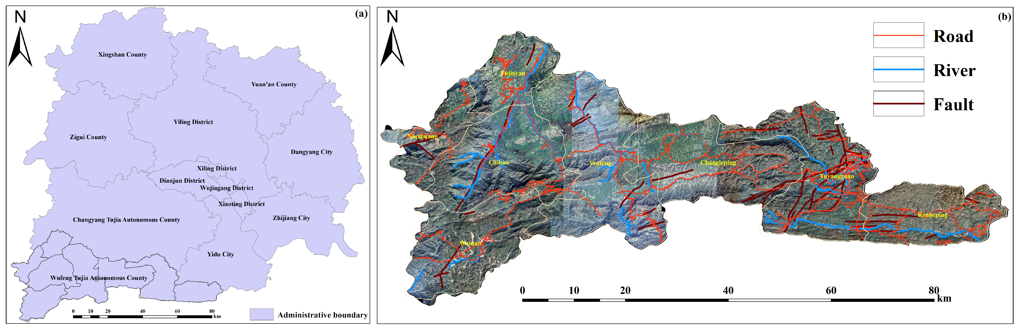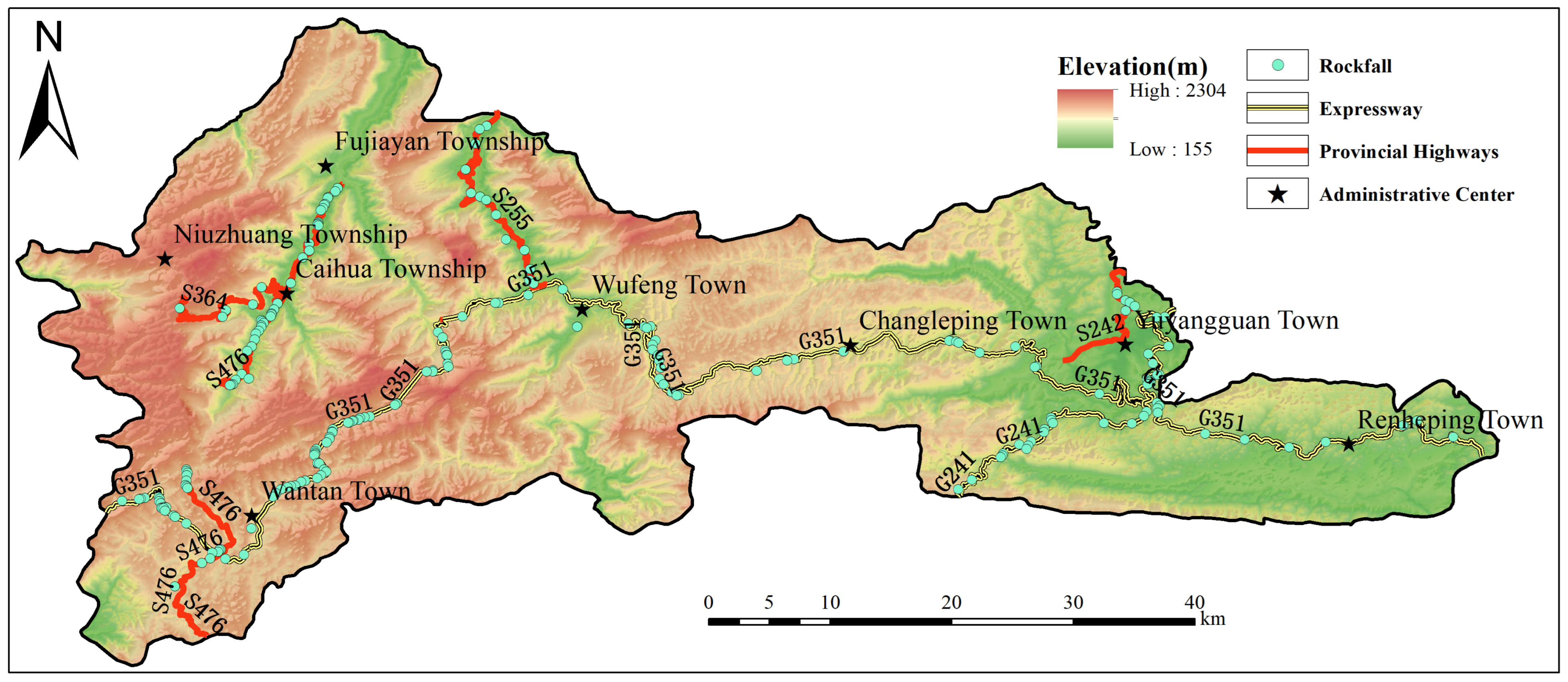In addition, the capability of regional emergency responses tends to be adversely affected by such incidents [6]. Wufeng Tujia Autonomous County is located in the fold-and-thrust zone of the Wuling Mountains of southwestern Hubei [7]. The area is deemed a classical region to study to determine rockfall hazards [8]. The regional geo-environmental system is inherently fragile, with complicated tectonic systems, steep topography and deeply incised valleys [9]. The quick development of the regional transport system, including national highways G351 and G241, has brought major anthropogenic perturbation to the geological environment [10,11]. Other provincial routes and expressways have also been included in the network. The initial stress condition of the hillside has been radically changed by engineering operations [12]. The large-scale removal of slopes is particularly important in this context. As a result, many unstable road cut slopes are produced [13]. These characteristics act as the main breeding grounds for future rockfall events.

There has been significant advancement in the area of susceptibility modeling. However, there are still a lot of uncertainties about choosing the right modeling scales [14]. The search for the best evaluation units to manage the hazards of roads remains a very important issue [15]. Dhakal et al. [16] assessed the vulnerability of road networks due to landslides in high-altitude mountainous areas and showed that machine learning models, in particular, Random Forest, can be successfully used to outline high-risk road sections. Tanoli et al. [17] introduced a modified Rockfall Hazard Rating System (RHRSP) to the high-relief transportation corridor by adding animal activity and road geometry parameters such as the shoulder width to improve the assessment of rockfall failure risk. An ensemble deep learning system combining CNN, DNN, and LSTM structures was proposed by Biswas et al. [18] to assess landslide susceptibility and develop a road vulnerability index, highlighting the synergistic effect of hydro-tectonic factors and anthropogenic pressure on infrastructure stability. Saldana et al. [19] contributed to the predictive maintenance of transport infrastructure by incorporating multi-source meteorological data and thermal measurements into an AI-based system, which enables the real-time detection of hazardous road surface conditions in various spatial domains. One of the main scientific goals of the present study is to study evaluation unit configurations systematically [20]. In this case, both raster and vectors are taken into consideration [21]. In addition, the independent predictive behaviors governed by the size of the spatial domain are systematically evaluated by cross-examining the macro-scale countywide baseline against localized transport corridor buffer footprints. Rather than asserting an unconstrained optimal spatial framework, this comparative analysis isolates how varying geographic boundaries, unit morphology shapes, and the newly introduced physics-informed indicator influence algorithmic boundary delineation. The primary objective of this research is to establish a controlled ablation and sensitivity evaluation matrix capable of quantifying the specific predictive contributions of the feature–unit interface. Crucially, the structural impacts of spatial autocorrelation leakage and sampling artifacts are rigorously controlled by implementing a strict Leave-One-Road-Corridor-Out Validation (LORCOV) protocol and a matched hard-negative screening matrix. By decoupling these interwoven geometric and mechanical effects across 13 benchmarking algorithms, this investigation aims to provide a calibrated, target-tiered decision-support matrix that assists transport authorities with localized public works resource allocation and proactive linear asset disaster mitigation.

The success of rockfall susceptibility mapping (RSM) depends on the choice of spatial evaluation units [22], which is the primary factor determining its effectiveness. The representativeness of conditioning factors is also viewed as an important controlling factor [23]. Raster units continue to be viewed as a common option in regional-scale evaluations [24] because of their computational power and retention of spatial continuity [25]. Nonetheless, it is still a major problem to directly link raster-based models to case-specific engineering mitigation approaches [26]. This challenge was tackled by Zhang et al. [27], who introduced an intelligent delineation of slope units using the stacking ensemble learning paradigm combining various machine learning paradigms and improved model interpretability using SHAP value analysis to assist in making more localized risk-informed decisions. Pokharel et al. [28] used a physically based method to create three-dimensional rockfall paths on mountain roads, enabling the creation of a segment-wise susceptibility index that can be correlated with geomorphological factors of initiation with discrete road corridors. Kong et al. [29] showed the importance of optimizing training samples in high-resolution modeling, showing that the synergy of surface roughness and road density is a critical multiplier in increasing hazards in transportation-intensive corridors. This was further developed by Noël and Nordang [30] by creating a quantitative hazard assessment structure that uses high-resolution models of 3D trajectories to assess the risk to mobile objects and fixed structures, thus closing the gap between simulated physical processes and particular infrastructure management requirements. Moreover, Giadrossich and Serra [31] incorporated the protective role of forest ecosystems and human-made barriers in a cost-oriented risk assessment model, measuring the amount of energy dissipated and economic loss to offer a replicable methodology to mitigate sustainable rockfall mitigation along transportation networks. Such models tend not to have the structure and functionality properties of infrastructure [32]. By way of contrast, vector units based on road units are considered to be a more practical solution for transportation management [33]. They are particularly oriented toward the linear geometry of the highway system. However, incorporating complicated geological and engineering concepts into a vector-based model continues to be very difficult [34]. During this integration, the statistical rigor necessary to implement machine learning should be ensured [35].

Another limitation comes with the extent of existing feature engineering [36]. Objective topographic elements play a significant role in the traditional susceptibility models [37]. The variables involve slope, elevation, and curvature [38]. Those factors are used in wide areas at the county scale [39]. According to Khan et al. [40], although the conventional model systems depend greatly on the typical topographical and hydrological inputs, it is essential to consider the inclusion of geomechanical parameters based on field observations, like the strength of rock mass, to be able to determine high-risk road cut slopes that cannot be detected using the macro-scale factors. According to Görüm et al. [41], long-term anthropogenic changes, especially highway engineering and quarrying, are long-term predisposing factors that cause gradual slope degradation, which finally leads to failure when exposed to modest environmental perturbation in a highly altered mountainous landscape. High-resolution DTMs based on LiDAR were used by Ellaithy et al. [42] to assess sediment connectivity, and they proved that road networks have the ability to change natural flow paths and sediment transport to a much higher degree than the natural topographic form, causing a greater impact on the density of landslides and localized susceptibility.

Nevertheless, the anthropogenic impact of road construction on the local environment may be missed by these factors [43]. Slope cutting has been identified as a major trigger of rockfall occurrence in mountains [13]. It tends to be masked in coarser-resolution raster data because of the natural smoothing of the terrain. Therefore, more sophisticated feature engineering is needed to mechanistically represent the effects of engineering excavations [44].

The fast development of machine learning and deep learning algorithms has brought a lot of model uncertainty to the field [45]. Other architectural designs have been used in hazard prediction over the past few years [46]. Such models include ensemble learning and complex neural networks [45]. Jiang et al. [47] pointed out that the accelerated growth of machine learning in the geosciences has the potential to be transformative regarding understanding processes; however, it is usually implemented without careful consideration and with methodological errors. These problems may result in deceptive interpretational findings and increase systemic uncertainty. Ikram et al. [48] performed a comparative analysis of conventional statistical models and machine learning models, comparing their predictive strength on high-relief landscapes because of the underlying constraints and predictive variability of various algorithmic methods. The internal and external decoupled graph convolutional network (IED-GCN) was proposed by Li et al. [49] based on super-pixel segmentation to address the problem of feature aggregation to achieve a much higher accuracy and stability of susceptibility assessment in complex space domains.

Nevertheless, the performance and robustness of these architectures are not very well understood [50]. Uncertainty is present at various spatial scales, including whole-county domains and narrow buffers [51]. There are also different observations with different types of units, such as raster and vector formats. A systematic and multi-scenario benchmark has not been documented in the literature. It is hard to provide reliable decision support in highway maintenance and disaster prevention without such a framework [52].

To address these interconnected methodological boundaries, this research establishes a comprehensive evaluation framework designed to simultaneously cross-examine the dependencies between spatial extent, mapping unit morphology, and physics-informed feature engineering for linear asset geohazard modeling. The developed approach partitions the computational workspace into five multi-scale spatial scenarios, implementing an object-oriented vector road evaluation unit (REU) network to resolve the scale artifacts typical of conventional grid cells. Furthermore, an anthropogenic disturbance proxy, defined as the theoretical slope-cutting height ($H_{\mathrm{cut}}$), is integrated within a controlled feature-ablation matrix to isolate the independent informational gain of mechanistic parameterization along excavated slope toes. By routing these configurations through an expanded benchmark of 13 statistical, machine learning, and advanced tabular deep learning architectures under strict Leave-One-Road-Corridor-Out Validation (LORCOV) spatial constraints, this workflow systematically decouples the interlocking predictive contributions of boundaries, shapes, and engineering descriptors. Multi-temporal SBAS-InSAR deformation tracking and stratified geomechanical field reconnaissance are subsequently utilized to execute post hoc external cross-examinations, evaluating the operational calibration and threshold performance of the localized vector platform for infrastructure risk mitigation.

2. Study Area and Data Sources

2.1. Study Area

Wufeng Tujia Autonomous County is situated in the southwestern mountainous region of Hubei Province, China. Geographically, the research area extends from longitudes 110°15′E to 111°25′E and latitudes 29°56′N to 30°25′N, encompassing an overall land area of 2372 square kilometers. The spatial location map and associated remote sensing imagery of the study area are illustrated in Figure 1.

2.1.1. Geomorphological Features

Physiographically, Wufeng County is characterized by an east–west-trending fold-and-thrust mountain system that forms a northern structural extension of the Wuling Mountains. The geomorphological landscape is dominated by deeply dissected tectonic-dissolution and erosional mid-mountain landforms. The structural elevation deflates sequentially across the workspace, ranging from a baseline low of 130 m to a peak threshold of 2289 m above sea level. This sharp topographic relief creates substantial localized gravitational potential energy and complex microtopographical gradients, providing critical boundary conditions for rock mass detachment. Based on genetic origin and spatial morphology, the regional geomorphology is classified into three distinct categories illustrated in Figure 2.

The regional landscape is structurally organized into three nested morphotectonic domains that directly control geohazard zoning. The central and southwestern sectors are dominated by high-relief tectonic-dissolution mid-mountains (1200–2300 m above sea level), where intense river incision has formed steep V- and U-shaped valleys with a maximum relative relief of 1800 m. This domain displays a pronounced altitudinal morphologic stratification: the upper tier (1200–2300 m) is characterized by vertical carbonate cliffs with inclinations of 70–90° and relative reliefs of 80–300 m, whereas the lower tier (under 1200 m) is composed of less steep Silurian clastic sequences.

The eastern and southeastern zones transition into mid-to-low mountains (500–1200 m above sea level), forming a typical karst peak-forest and dissolution trough system within Cambrian to Ordovician carbonates. Lastly, the low-altitude hilly areas (under 500 m) are localized around the Yuyangguan and Fengxiangping zones. Tectonically controlled by the intersection of the Yuyangguan and Xiannvshan fault complexes, the Paleozoic strata within these low-lying zones exhibit intense structural deformation and disorganized bedding orientations. Across these three domains, the widespread presence of oversteepened engineered cut slopes, interbedded hard carbonate and soft argillaceous sequences, and thick colluvial–deluvial aprons at the slope bases establishes highly favorable geomechanical preconditions for structural stress relief, progressive rock mass fracturing, and subsequent rockfall initialization.

2.1.2. Geological and Tectonic Setting

Tectonically, the study workspace is situated within the fold-and-thrust belt of the western Hubei mountains, which constitutes a structural sector of the Yangtze Craton. The stratigraphic succession is dominated by Paleozoic marine sedimentary sequences, primarily characterized by thick-bedded, competent carbonate formations—such as limestone and dolomite—interbedded with incompetent sandstone and fissile shale strata (Figure 3). Persistent tectonic stresses have induced highly developed, persistent structural discontinuities, including conjugated joint networks and structural karst fractures within the carbonate matrices. These intersecting discontinuity planes structurally segregate the parent rock mass into discrete, potentially unstable block clasts, establishing the prerequisite geological constraints for rockfall initialization. Crucially, the extensive construction of the transportation network acts as an intense anthropogenic perturbation; aggressive technical slope-toe excavations have artificially oversteepened the slope profiles, disrupting the downstream basal boundary support and accelerating stress-relief fracturing along these engineered corridors.

2.1.3. Climate and Hydrology

The study region is characterized by a subtropical humid monsoon climate regime, exhibiting a pronounced spatial gradient with annual precipitation ranging from 1064 mm to 1919 mm. Heavy rainfall is temporally concentrated in April to September, which typically encompasses over 80% of the annual moisture input. Under the influence of intense seasonal rainstorms, fast surface runoff frequently infiltrates the highly developed structural joint corridors of the engineered cut slopes. This localized hydrological infiltration elevates transient pore water pressures along persistent discontinuities and induces severe slaking actions within the soft argillaceous interlayers, effectively reducing the shear strength of the rock mass boundaries.

The regional hydrographic network is controlled by the Qingjiang and Lishui drainage systems, comprising mountain river networks characterized by high discharge sensitivity to short-duration precipitation intensity. Combined with aggressive anthropogenic slope-toe excavations, this seasonal water-enrichment process acts as a primary dynamic triggering mechanism that accelerates stress-relief propagation and progressive structural unroofing, driving frequent rockfall initialization along the active transportation corridors during the monsoon period.

2.1.4. Road Network

The regional transportation infrastructure matrix within Wufeng County comprises a tiered network categorized into national, provincial, and local road systems. The structural spine of this transit network is defined by major linear corridors, including national highways G351 and G241, alongside key provincial trunks such as S242 and S255. Due to the highly dissected mountain topography, the alignment configurations of these existing lifelines are characterized by extensive engineering slope-toe excavations. This widespread anthropogenic cutting across brittle stratigraphic sequences creates numerous high-vertical rock cut profiles, generating the primary localized engineering registries evaluated within our multi-scenario computational framework. The location of national and provincial roads in the study region is shown in Figure 4.

2.1.5. Inspection of Geological Disasters Along the Road Sections

An initial evaluation consisted of a thorough examination of the area’s geological context and the geohazard history of the region. Multi-source data on which the research was based incorporated the usage of remote sensing satellite imagery and 1:250,000 geological maps as the primary spatial framework. Identification of rockfall risks in highway corridors was completed through a combined methodology that included Unmanned Aerial Vehicle (UAV) photogrammetry and systematic field geological surveys. This study considered six trunk roads, including two national and four provincial trunks, with a total survey distance of 346.41 km. In total, 220 rockfall hazard locations were found along the investigated routes, and their spatial occurrence is described in detail in

Table 1. Distribution statistics of road collapse geological disasters.

Road	Mileage/km	Number of Rockfall Disaster Sites	Density (Number/km)
G351	177.36	118	0.66
G241	46.23	30	0.65
S242	16.03	6	0.37
S255	27.82	13	0.47
S364	42.00	22	0.52
S476	36.97	31	0.84

and presented in Figure 5.

The rockfall hazards are located at different road sections of Wufeng County, and there have been 118 incidents on the G351 highway alone. This number is much higher than the frequencies of other routes examined, making G351 a high-frequency channel of rockfall hazards. Conversely, incidences reduce significantly on G241, S476 and S364, with 30, 31 and 22 incidences, respectively, and the fewest occur on the S255 and S242 routes. S476 has the greatest linear density. The investigated corridors in descending order of linear density are: S476, G351, G241, S364, S255, and S242.

Table 2. Statistics of collapse development characteristics.

Classification Criteria	Type	Number of Rockfall Disaster Sites	Percentage%
Slope (°)	<45	1	0.45%
	45–60	14	6.36%
	60–75	47	21.36%
	≥75	158	71.82%
Material composition	Limestone	126	57.27%
	Sandstone	45	20.45%
	Mudstone	49	22.27%
Deformation and failure modes	Sliding	75	34.09%
	Toppling	50	22.73%
	Falling	76	34.55%
	Tension cracking	19	8.64%
Stability status	Stable	1	0.45%
	Basically stable	215	97.73%
	Unstable	4	1.82%
Rockfall scales	Small (<1 × 103 m3)	214	97.27%
	Medium (1 × 103~1 × 104 m3)	6	2.73%
The threatened road length (m)	<100	118	53.64%
	100–200	72	32.73%
	200–300	22	10.00%
	≥300	8	3.64%

summarizes statistical properties of the 220 hazard spots located on these national and provincial highways.

The compiled empirical inventory reveals distinct geomechanical development characteristics and highly structured spatial distribution patterns for the 220 documented rockfalls across Wufeng County. Structurally, the historical failures are predominantly characterized as small- to medium-scale translational and toppling rockfalls, with volumetric thresholds typically ranging from 10 to 500 cubic meters. Morphologically, these instabilities are extensively localized along vertical or near-vertical engineered cut slopes, with pre-failure inclinations concentrated between 65° and 85°. Geomechanically, the detached blocks are tightly governed by planes with persistent structural discontinuity, notably, conjugating tectonic joints and unloading fractures that intersect the bedded marine Paleozoic carbonate and shale sequences, triggering severe stress-relief propagation, progressive rock mass loosening, and subsequent gravity-driven detachment.

Spatially, the historical rockfall occurrences exhibit a highly non-uniform, clustered distribution pattern, tightly coupled with an intense anthropogenic footprint and specific geomorphological parameters. First, a striking linear proximity effect is documented along the primary transit alignment: 87.3% (192 sites) of the documented rockfalls are clustered within a narrow 50 m corridor immediately bounding national highways G351 and G241 and provincial highways S242 and S255, mathematically demonstrating that technical slope-toe cutting represents the primary engineering trigger across the landscape. Second, altitudinally, 74.1% of the failure loci are concentrated within the mid-mountain structural tier between 800 and 1500 m above sea level, aligning directly with the geographic domains characterized by intense fluvial dissection and high macro-scale relief energy. Third, regarding lithological partitioning, 68.6% of the events are situated within Cambro–Ordovician limestone formations interbedded with fissile Silurian shales, where pronounced differential weathering systematically unroofs the structural support of the overlying competent rock columns, resulting in high-density hazard hotspots along deeply cut river valleys and winding mountainous highway corridors.

2.2. Evaluation Factors and Data Sources

2.2.1. Data Sources

The choice of evaluation factors is a vital step in rockfall susceptibility mapping (RSM) because predictive accuracy and performance of machine learning models depend on the quality and relevancy of the input features. During this study, 12 conditioning factors were chosen and arranged in five main thematic directions, namely, topographic, geological, environmental, hydrological, and engineering. All the features were based on multi-source datasets, which were then processed to be compatible with the modeling framework defined previously. The list of the selected conditioning factors is presented in

Table 3. Summary of data sources and evaluation factors.

Category	Evaluation Factor	Data Source	Resolution
Topography	Elevation, slope, aspect curvature, Terrain Ruggedness Index surface roughness Topographic Wetness Index	ALOS PALSAR DEM	12.5 m
Geology	Lithology, distance from the fault	Geological Map	1:50,000
Environment	NDVI	Landsat-8 OLI	30 m
Hydrology	Distance from the water system	Water system data	1:50,000
Engineering	Land use	CLCD (Wuhan University)	30 m

.

2.2.2. Factor Preparation

The spatial distribution of the 12 conditioning factors that were used in this research is shown in Figure 6. The factors include topographic, geological and environmental dimensions that are effective in describing the mechanisms that control the susceptibility of rocks to falling. The evaluation was conducted based on the main interest in the vital road corridors of Wufeng County so as to make sure that the chosen variables could suit the particular geo-environmental situations of the research area.

(1)

Topographic Factors

Topography is the fundamental driving force behind rockfall events. The gravitational potential energy can be defined by assessing the topographic characteristics. Moreover, the influence of such characteristics regulates the kinematic possibility of block detachment.

Elevation: The elevation is used as a proxy of complicated climatic and vegetation vertical zonation. Intense freeze–thaw processes are often noted in higher elevations in Wufeng County. These elevated areas are also characterized by strong physical weathering. Such processes can lead to a significant increase in the rates of fragmentation of rock masses. Figure 6a shows the Digital Elevation Model (DEM) and the topographical features of Wufeng County. There is a considerable gradient in the west-to-east direction in the terrain that has an elevation reading between 155 m and 2304 m. Such a high relief creates a diverse landscape that has great spatial heterogeneity.

Slope: Slope angle directly governs the distribution of shear and normal stresses acting on rock masses, serving as a primary controlling factor in rockfall mechanics. The spatial distribution of slope angles in Wufeng County ranges from 0° to 79.04° (Figure 6b), featuring numerous steep slopes sharper than 45°. These precipitous topographic features provide the necessary kinetic gradient to induce the rapid acceleration of detached rock blocks.

Aspect: Slope aspect is a determinant variable influencing the distribution of solar radiation and the impact of prevailing winds in mountainous ecosystems. Differences in slope aspect lead to heterogeneous moisture evaporation and temperature fluctuations, which significantly affect weathering intensity and promote joint propagation within the rock mass. As shown in Figure 6c, the slope aspect in Wufeng County is categorized into four primary quadrants: 0–90°, 90–180°, 180–270°, and 270–360°.

Curvature: This parameter represents the convergence or divergence of terrain morphology, directly influencing surface hydrological processes and internal stress redistribution within hillsides. Concave and convex slopes regulate the concentration and routing of surface runoff, thereby altering localized slope stability. The spatial distribution of curvature across Wufeng County is illustrated in Figure 6d.

Terrain Ruggedness Index (TRI): TRI quantifies the relative topographic relief between adjacent pixels, acting as an indicator of highly dissected and fragile geomorphological settings where rockfalls frequently occur. The spatial pattern of TRI in Wufeng County ranges from 0 to 397 (Figure 6e), with elevated values corresponding to zones of intense structural dissection.

Surface Roughness: Defined as the ratio of the surface area to its horizontal projection, surface roughness serves as a fundamental metric to describe the morphological complexity of the slope face. This factor dictates the frictional resistance and kinetic behavior (such as bouncing or sliding modes) of detached rock blocks during runout. In Wufeng County, surface roughness varies between 1.00 and 5.26, as depicted in Figure 6f.

Topographic Wetness Index (TWI): TWI is a critical hydrological indicator that quantifies the spatial distribution of soil moisture and groundwater accumulation. High TWI values denote potential zones of increased pore water pressure, which reduces the effective stress along rock joints and acts as a key initiation mechanism for rockfall failures. The spatial distribution of TWI in Wufeng County ranges from 6.32 to 45.83 (Figure 6g).

(2)

Geological Factors

Geological conditions are recognized as a material cause of rockfall occurrence. Geological factors also provide structural control in the study area.

Lithology: There are significant differences in the physical and mechanical properties of the rock units throughout the study region. The properties are rock hardness and bedding structures. Carbonate rocks and clastic sequences have different susceptibilities to weathering. Such variations in lithology also affect gravitational detachment. Figure 6h shows the spatial arrangement of the lithological units in Wufeng County. Major differences are noted in the physical and mechanical properties of these rock units, especially in rock hardness, bedding structures, and resistance to weathering. Lithology is divided into six categories depending on their geological features:

Soft-plastic and loose-to-moderately-dense sandy gravely soil: It is mainly found in valleys having low mechanical strength.

Hard-to-very-hard thick-bedded massive quartz sandstones: High compressive strength and structural integrity are their characteristics.

Bedded soft-to-medium-thick sandstone, mudstone and shale alternated with thin-to-medium-thick bedded sandstone and argillaceous limestone: The bedding is well developed and is highly prone to weathering.

Hard, thick-bedded, massive, strongly karstified lithological group: Defined by intense karstification and secondary porosity.

Difficult-to-moderately-difficult, medium-to-thick-bedded, intensely-to-moderately-karstified limestone and argillaceous limestone intercalated with soft shale: Very heterogeneous and lithologically varied.

Largely hard, thin-to-medium-thin bedded with minor karstification of the argillaceous carbonate rocks interbedded with slate: It is marked by clear structural deformation.

Distance from faults: Tectonic activity creates fracture zones. These structural zones have higher joint density as well. Highly fragmented rock masses are commonly found near the faults. These materials also have lower shear strength. As a result, the occurrence of rockfall is greatly heightened due to these structural factors. Figure 6i shows the distance between tectonic faults in space in Wufeng County. This parameter is classified by 50 m intervals ranging between 0 m and above 1000 m. Fracture zones arise due to tectonic activity, which causes an increase in joint density in these structural zones.

(3)

Environmental Factors

NDVI: The density and vigor of vegetation cover within the study area is characterized by the normalized difference vegetation index. This index is also identified as NDVI. The differential reflectance of vegetation in the red and near-infrared spectral bands is utilized for the calculation of this index. The following formula is defined for the calculation process.

$$\mathrm{NDVI}={\displaystyle \frac{NIR-Red}{NIR+Red}}$$

(1)

In this expression, the surface reflectance in the near-infrared and red bands is represented by $NIR$ and $Red$, respectively. NDVI values were derived from multi-temporal Landsat-8 OLI imagery for the current investigation. A spatial resolution of 30 m was associated with the original imagery. These data were subsequently resampled to match the 12.5 m analysis grid. Figure 6j presents the spatial distribution of vegetation coverage across Wufeng County, with values ranging from 0 to 1. The normalized difference vegetation index (NDVI) was utilized to quantify the vegetation density within the study area.

(4)

Hydrology Factors

Distance from the water system: The distance from the water system has been used as a main hydrological proxy. The role played by fluvial processes in the stability of nearby slopes was evaluated using the given factor. The measure of the given variable was obtained using the Euclidean distance calculation. It was calculated between the digitized drainage network and every evaluation unit. The Yuyang, Tianchi and Siyang rivers were part of the digitized network in the present case. Figure 6k represents the spatial variation of the distance from the water system in Wufeng County. This factor is included as a leading hydrological proxy to specify the effect of fluvial processes on the stability of adjacent slopes. This variable was quantified based on the measurement of the Euclidean distance between the digitized drainage network and each evaluation unit, with 50 m intervals being used to spatially group them.

(5)

Engineering Factors

The Land Use and Land Cover (LULC) factor was integrated in order to capture the degree of anthropogenic activity and the relative levels of surface stability across the study area. The CLCD is a China Land Cover Dataset (CLCD) created by the research group of Wuhan University. This dataset is based on multi-temporal Landsat imagery available on the Google Earth Engine (GEE) and has a spatial resolution of 30 m. To be consistent with the rest of the geo-environmental variables, the LULC layer was re-sampled to a 12.5 m grid with the nearest neighbor interpolation algorithm. The spatial distribution of the Land Use and Land Cover (LULC) across Wufeng County is shown in Figure 6l. Crucially, the potential artificial boundary noise introduced by the sub-pixel edge alignment during this 30 m to 12.5 m transformation is effectively neutralized across the high-resolution 1 km road buffer environment. Within our computational pipeline, the pixel-level environmental attributes are not ingested directly by the machine learning classifiers as raw cells; instead, they are spatially aggregated into the object-oriented vector road evaluation units (REUs) via zonal statistics mapping. When the zonal majority for the categorical land use vectors and the zonal mean for the continuous NDVI arrays are calculated across each discrete road segment, the localized blocky geometric steps are smoothly distributed and filtered out, preventing artifact-driven feature variance and ensuring an uncorrupted parameter input matrix. The LULC factor was included because it describes the intensity of anthropogenic activity as well as the different levels of surface stability of different cover types. The categories defined in the study area are cropland, forest, shrub, grassland, water, barren, and impervious surfaces. Forest is the largest land cover type, whereas impervious surfaces depict the size of built-up areas and infrastructure, indicating the impact of human activity on the landscape.

The resampling of all continuous variables was performed at a spatial resolution of 12.5 m to be consistent with the ALOS PALSAR DEM. In order to describe the most critical geomechanical conditions of road cut slopes, the pixel-level information on 550 road-segment evaluation units was summed up using maximum and mean operators in the uphill buffer zones.

2.2.3. Multicollinearity Analysis

The presence of multicollinearity between conditioning factors in rockfall susceptibility modeling may cause model instability and overfitting because redundant information increases the variance in estimated coefficients. To ensure that the input predictors are sufficiently decollinear for the current workflow, a multicollinearity diagnosis was conducted based on the Variance Inflation Factor (VIF). Per accepted statistical conventions, a VIF greater than 10 indicates severe multicollinearity that requires structural feature mitigation. Figure 7 and

Table 4. Multicollinearity diagnosis and Variance Inflation Factor (VIF) values for the initial and retained rockfall conditioning factors.

Factor Name	Initial VIF	Retained VIF
Distance from the fault	1.10	1.10
Distance from the water system	1.285	1.281
Elevation	1.419	1.414
Slope	16.767	Removed
Aspect	1.002	1.002
Curvature	1.003	1.00
Vegetation coverage	1.13	1.133
Lithology	1.026	1.021
Terrain Ruggedness Index	17.523	Removed
Surface roughness	9.191	1.909
Topographic Wetness Index	5.183	1.935
Land use	1.001	1.00

show the preliminary diagnostic findings on the 12 candidate factors. Significant multicollinearities were detected between slope (VIF = 16.767) and the Terrain Ruggedness Index (TRI, VIF = 17.523), indicating highly redundant topographic information within the geomorphological framework of Wufeng County.

Additionally, surface roughness and the Topographic Wetness Index (TWI) initially displayed elevated VIF values of 9.191 and 5.183, respectively. Despite approaching the critical baseline, both variables were explicitly retained in the candidate pool due to their indispensable geomechanical and hydrological representation in linear asset engineering contexts. Surface roughness parameterizes macro-scale rock mass structural degradation and localized block detachment potential along excavated slopes, while TWI functions as a primary indicator of localized groundwater concentration and pore water pressure fluctuations that trigger structural slope-toe failure.

To optimize the feature space, a stepwise elimination approach was adopted whereby slope and TRI were excluded. After removing these two redundant predictors, the VIF metrics of the remaining 10 factors were re-evaluated. As illustrated in Figure 7, structural multicollinearity was effectively suppressed. The VIF values of all remaining variables, including elevation, aspect, and curvature, dropped well below 2.0, with the maximum records stabilized at TWI of 1.935 and surface roughness of 1.909. These findings demonstrate that the selected evaluation factors are sufficiently decoupled from collinearity constraints, establishing a mathematically sound and stable data foundation to train the subsequent 13 machine learning and deep learning models.

Therefore, executing a stepwise VIF-driven elimination loop successfully prunes these redundant parameters, dropping the maximum system VIF baseline below 2.45 and ensuring structural parameter independence. This data-driven de-biasing underpins the design of our vector REU feature-ablation states; selectively stripping slope and TRI within specific control loops does not render the learner blind to slope anomalies but rather represents a calibrated approach to prevent collinearity inflation while leveraging independent engineering proxies like the theoretical slope-cutting height ($H_{\mathrm{cut}}$).

2.2.4. Factor Correlation Analysis

In order to explore the internal relations between the conditioning factors in more detail, the Pearson product-moment correlation coefficient (r) was used to perform a pairwise linear correlation analysis. Although the analysis of VIF dealt with multi-dimensional collinearity, the Pearson matrix offers a detailed view of the covariance between every two factors.

Figure 8 shows the correlation matrices prior to and after eliminating redundant factors. In the first matrix (Figure 8a), there was a large degree of redundancy among the topographic variables. In particular, slope had very high positive correlations with the Terrain Ruggedness index (TRI) (r = 0.94, p < 0.01) and surface roughness (r = 0.88, p < 0.01). Moreover, there were high negative correlations between slope and the Topographic Wetness Index (TWI) (r = −0.88, p < 0.01) and between TRI and TWI (r = −0.79, p < 0.01). Such high coefficients (|r| > 0.7) indicate that these topographic factors represent almost the same geomorphological features and may, therefore, introduce bias into the weight assignment and affect the predictive ability of machine learning models.

After the slope and TRI are eliminated, the correlation matrix that has been fine-tuned in Figure 8b shows a much better feature independence. All the pairwise correlation coefficients in this optimized feature set were less than the critical value of 0.7. The smallest correlation was obtained between surface roughness and TWI (r = −0.69, p < 0.01). It is negatively correlated, which is geomorphologically consistent because steeper and rougher terrains tend to promote quick surface runoff and prevent the local accumulation of moisture. There were other variables, including elevation and distance to water system, that had only a moderate correlation (r = 0.44, p < 0.01), and variables like aspect, curvature, and land use were almost uncorrelated with all other factors.

As shown in the transition between the first and the second matrix, the removal of slope and TRI does effectively curb statistical noise induced by topographic redundancy. This statistically significant feature space will allow the 11 machine learning and deep learning algorithms to better identify unique patterns in each of the factors, thus improving the interpretability and generalization behavior of the rockfall susceptibility maps.

3. Methodology

3.1. Overall Algorithmic Framework

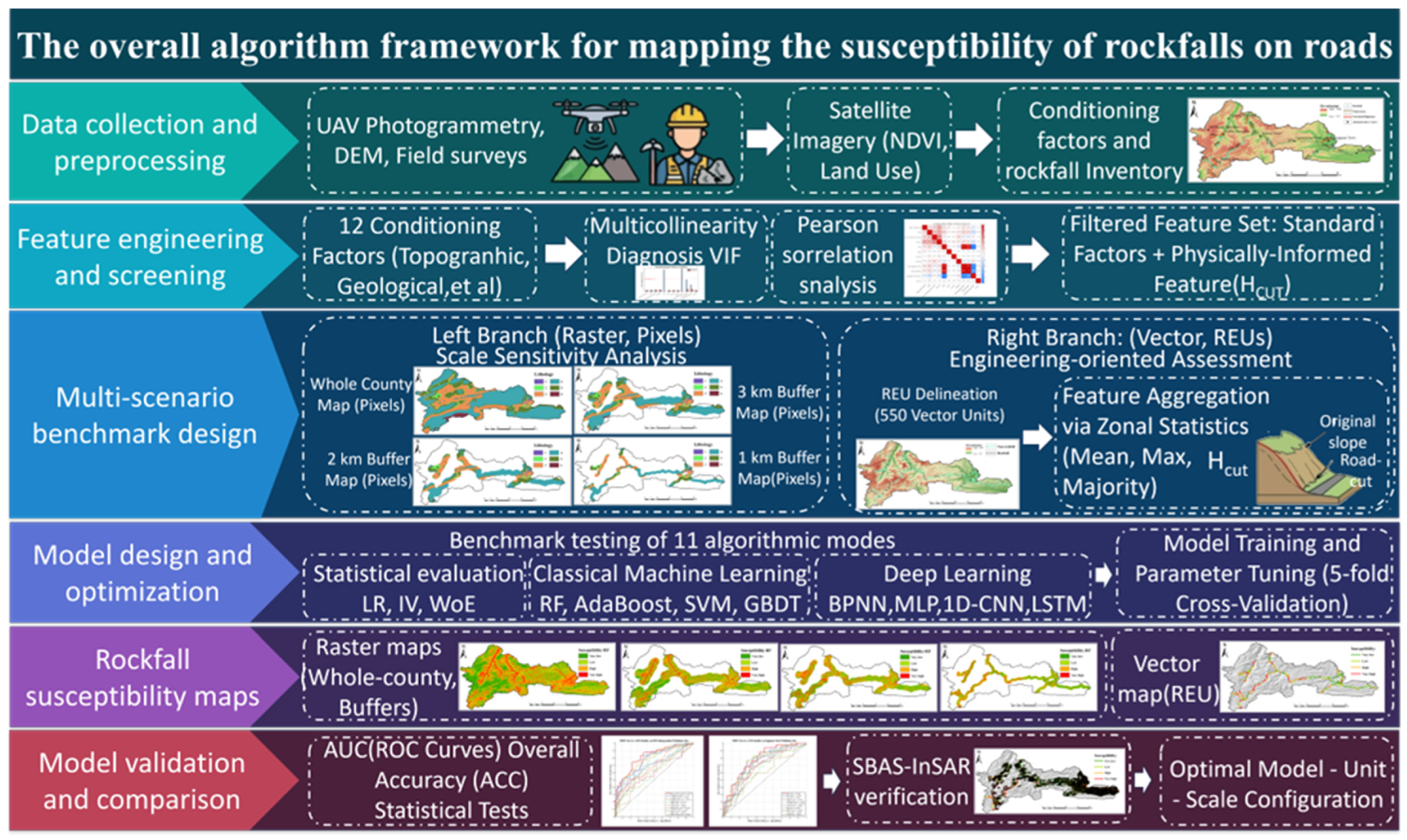
The systematic framework of rockfall susceptibility mapping (RSM) proposed in the present work is depicted in Figure 9. In order to resolve the uncertainties that come naturally with spatial evaluation units and modeling scales, an overall algorithmic system was created that involved six consecutive steps, starting with multi-source data collection and ending with final validation.

Stage 1: Data Collection and Pre-processing

Starting with the combination of high-fidelity field survey records, Unmanned Aerial Vehicle (UAV) photogrammetry, Digital Elevation Models (DEMs), and multi-spectral satellite images, the primary geospatial framework is established. These multi-source datasets are utilized to compile a validated rockfall inventory consisting of 159 positive and 391 negative samples while deriving 12 preliminary geo-environmental conditioning factors.

Stage 2: Feature Engineering and Screened Ablation

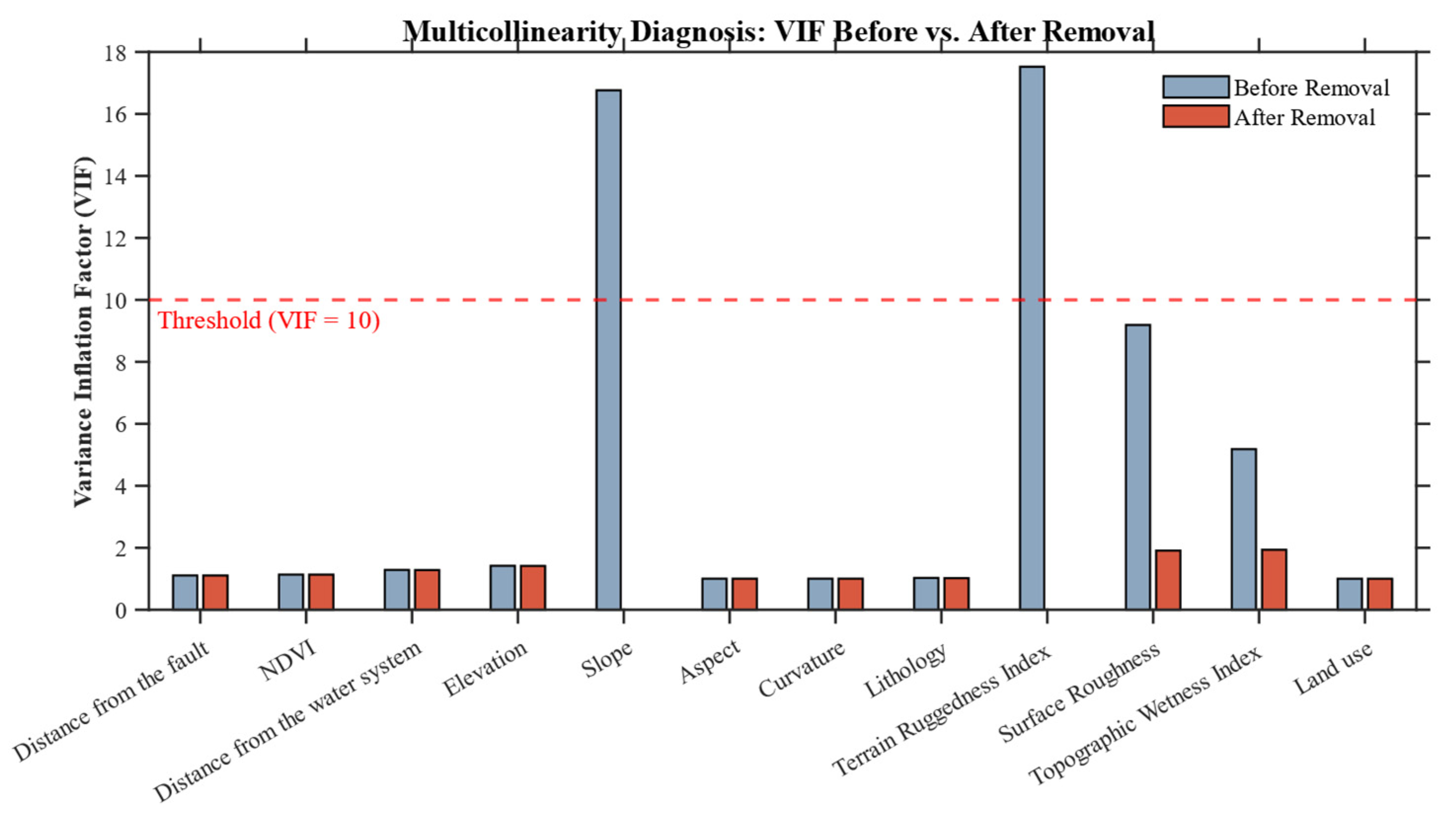
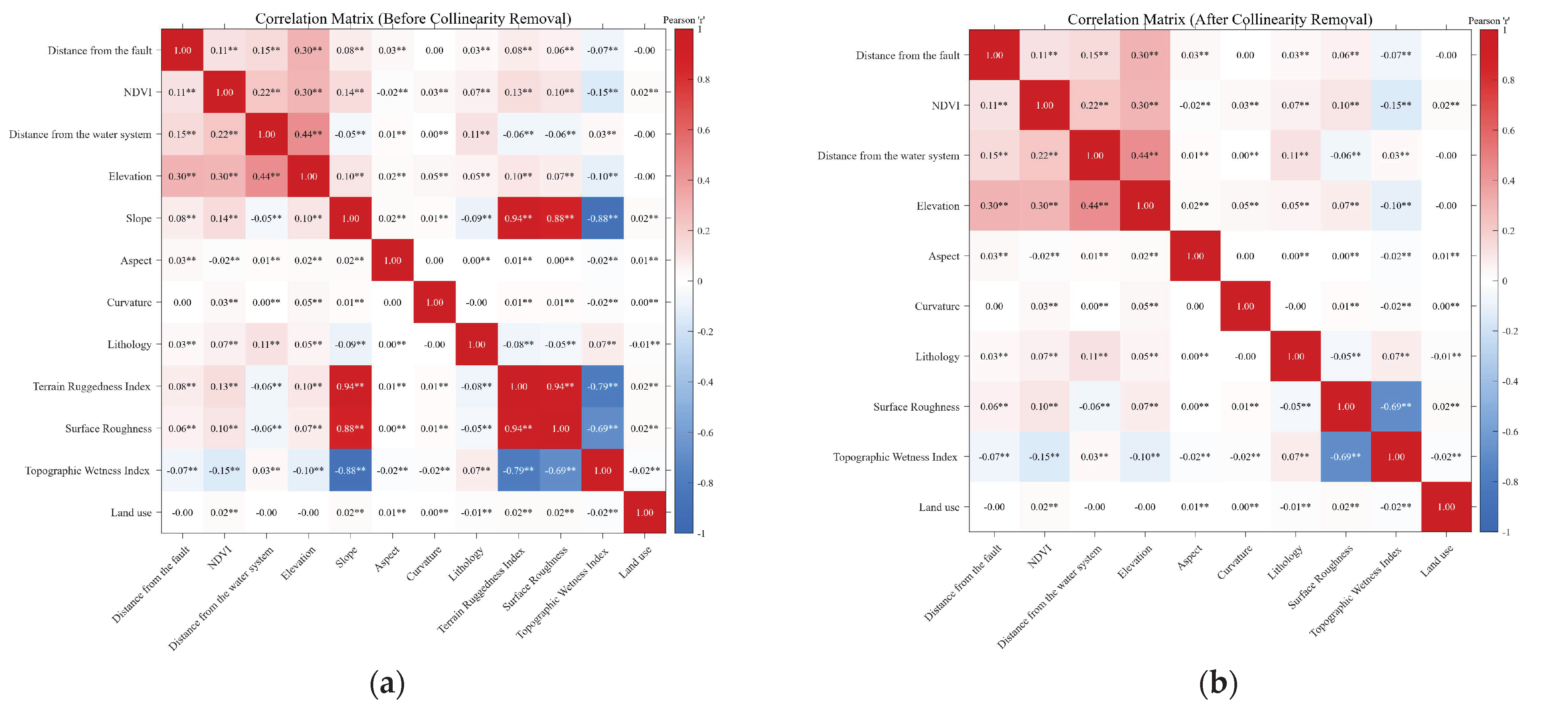
A rigorous feature screening and ablation protocol is executed to evaluate the explicit effects of feature engineering independent of geometric configurations. To suppress redundant topographic structures and establish a decollinearized attribute space, a multicollinearity diagnosis based on Variance Inflation Factor (VIF) analytics is implemented. Crucially, as a core feature engineering perturbation, a novel physically informed indicator defined as the theoretical slope-cutting height ($H_{\mathrm{cut}}$) is introduced exclusively within the vector-based workspace to parameterize anthropogenic excavation footprints. To isolate the independent informational weight of this proxy, the feature engineering phase establishes both a full-featured matrix and a feature-minimalist ablation variant, enabling the subsequent benchmarks to explicitly measure the predictive gain of mechanistic parameters.

Stage 3: Multi-scenario Benchmark Design

The operational architecture partitions the experimental workflow into a systematic comparative grid designed to simultaneously cross-examine three separate questions: the effect of the spatial extent, the effect of the mapping unit, and the effect of feature engineering. First, to test the effect of the spatial extent, the workflow bifurcates the analysis into a macro-scale whole-county domain and three localized road-centric corridors restricted to 1 km, 2 km, and 3 km buffers. Second, to evaluate the effect of the mapping unit, the framework contrasts continuous cellular grids against an object-oriented vector workspace composed of 550 road evaluation units (REUs), where pixel-level conditioning factors are aggregated into homogeneous segments via spatial zonal statistics. Third, by routing these unit-extent scenarios through the ablated feature configurations across 13 benchmarking algorithms under both unconstrained splits and strict Leave-One-Road-Corridor-Out Validation (LORCOV) constraints, the benchmark systematically decouples the interlocking predictive contributions of boundaries, shapes, and engineering descriptors.

Stage 4: Model Design and Optimization

This paper applies a large-scale benchmark testing of 11 representative algorithmic models. The models are sorted into statistical evaluation paradigms (LR, IV, and WoE), classic machine learning algorithms (RF, AdaBoost, SVM, and GBDT) and more recent deep learning systems (BPNN, MLP, 1D-CNN, and LSTM). Hyperparameter optimization is performed on each model through 5-fold cross-validation to achieve best generalization abilities on the 55 experimental designs.

Stage 5: Rockfall Susceptibility Mapping and Zonation

Following model calibration across the multi-scenario baseline and ablated feature workspaces, the continuous rockfall susceptibility index is derived for each operational scenario. This stage generates a sequence of high-resolution macro-scale raster maps covering the entire county and its localized corridor buffers, alongside the vector-based classification fields computed within the homogeneous road evaluation units (REUs), to parameterize the sharp geomechanical hazard gradients adjacent to active cut slopes.

Stage 6: Multi-Metric Validation and External Calibration

The final phase executes a rigorous quantitative assessment across the 65 model-scale-unit base configurations. Threshold discrimination and spatial generalization capacity are systematically audited using the area under the curve (AUC) of receiver operating characteristic (ROC) trajectories, precision–recall metrics, and overall accuracy parameters under both randomized splits and strict Leave-One-Road-Corridor-Out Validation (LORCOV) spatial block boundaries. To provide post hoc physical support and evaluate the alignment between algorithmic risk probabilities and empirical slope displacement, the susceptibility outputs are subjected to an external cross-examination against multi-temporal SBAS-InSAR deformation velocity fields. By applying non-parametric Kruskal–Wallis testing and Spearman rank correlation modeling, this stage establishes a formal statistical connection between computed hazard levels and real-world ground displacement magnitudes, confirming the practical engineering utility of the localized vector mapping platform.

3.2. Multi-Scale Spatial Partitioning

This section describes in detail the methodology that was used to develop the hierarchical spatial domains. Multi-scale partitioning strategy is applied to assess the sensitivity of the scale to the 11 algorithmic paradigms and identify the most suitable spatial scale at which rockfall susceptibility maps are to be prepared specifically with respect to the road corridor.

The spatial extent of the training and evaluation regions are very influential on the predictive performance of susceptibility models. On mountainous lands, although a whole-county assessment offers a macro-scale view, it can easily contain large parts of stable terrain where the model sensitivity to road-oriented hazards may be weakened. Alternatively, too small buffers can be used that would not cover important upslope incubation sites of rockfalls. Thus, it is necessary to utilize a multi-scale method in order to identify the so-called zone of influence where geological–morphological and engineering considerations play the most active role in the assessment of rockfall risks along the transportation network.

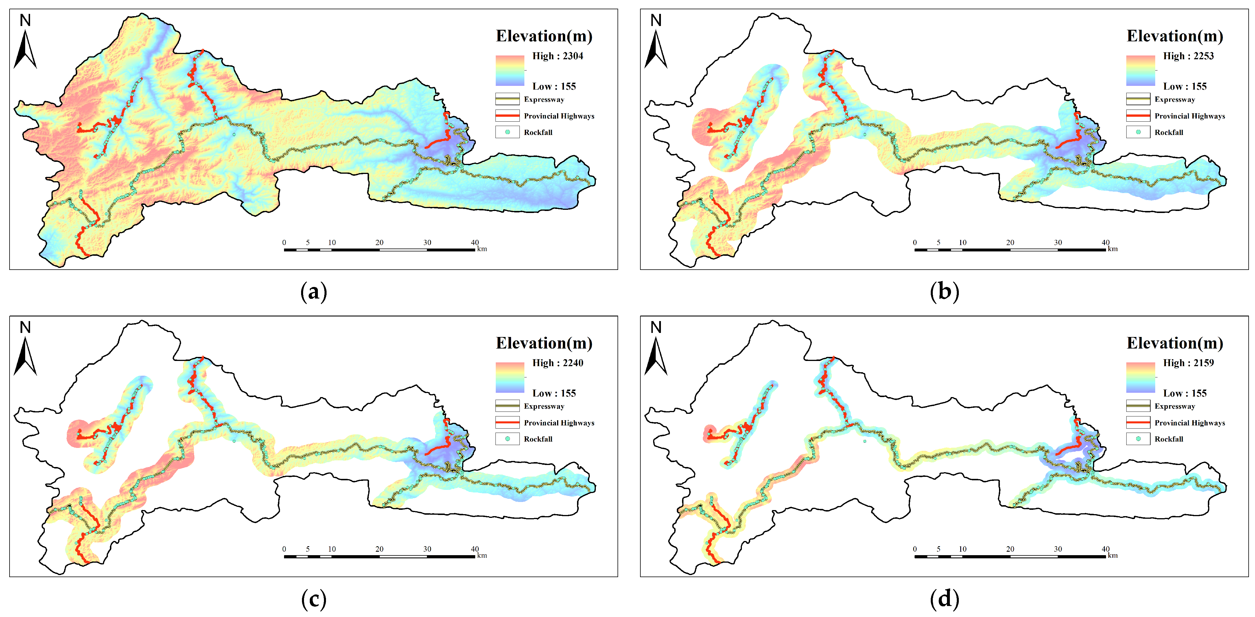
As shown in Figure 10, there are four unique raster-based scenarios that were created with the same spatial resolution of 12.5 m so as not to compromise the integrity of the cross-scale comparison:

The domain is the whole administrative area of Wufeng County, and the elevation value is between 155 m and 2304 m. The domain acts as a foundation of regional hazard zoning and enables assessment of the performance of models under the widest variety of geomorphological environments. There are altogether 159 rockfall events in the region concentrated in the valleys and cut slopes in large numbers.

Figure 10b: 3 km Road Buffer Scenario. The given domain restricts the analysis to a 3 km catchment area which is adjacent to the national and provincial highways network where the elevation varies between 155 m and 2253 m. It expands the analysis to regional ridge-and-valley systems, with larger topographic limitations that lead to slope instability.

Figure 10c: 2 km Road Buffer Scenario. The intermediate domain limits the assessment to a 2 km buffer region of the corridors, which has an elevation level between 155 m and 2240 m. The aim of this scale is to cover the intermediate slopes and secondary drainage basins that are actively affecting the stability of the main transportation routes.

Figure 10d: 1 km Road Buffer Scenario. The smallest area is the closest road corridor with up to 1 km buffer, in which the highest elevation is 2159 m and the lowest is 155 m. All of this is concentrated solely on the most direct interaction of the anthropogenic engineering works (road cutting) and the nearest natural relief.

3.3. Road Evaluation Unit (REU) and Physical Feature Engineering

3.3.1. REU Partitioning and Labeling Logic

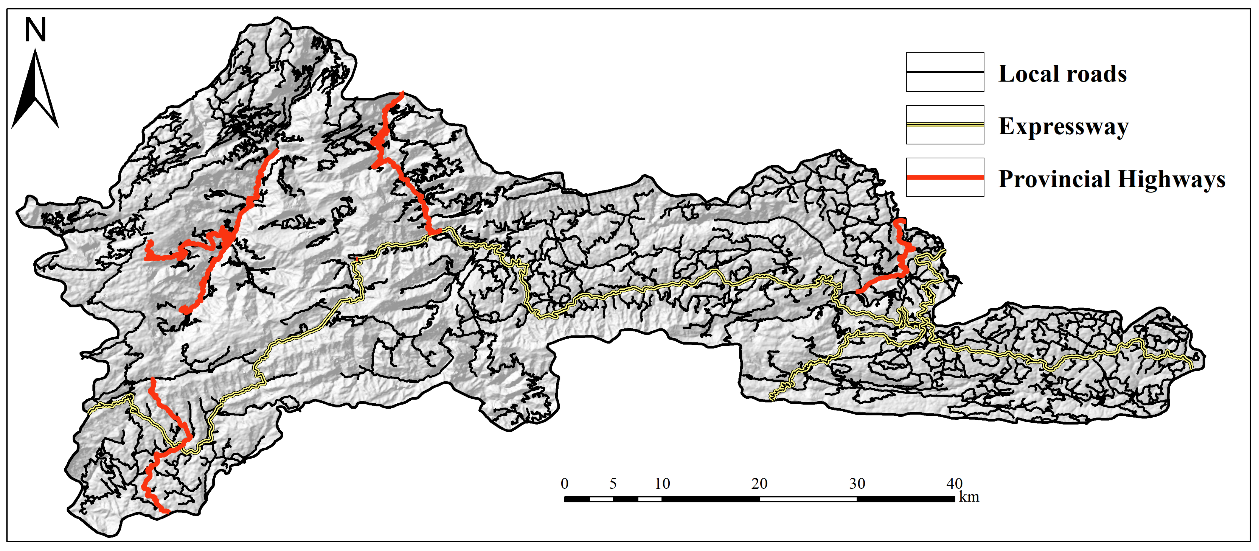
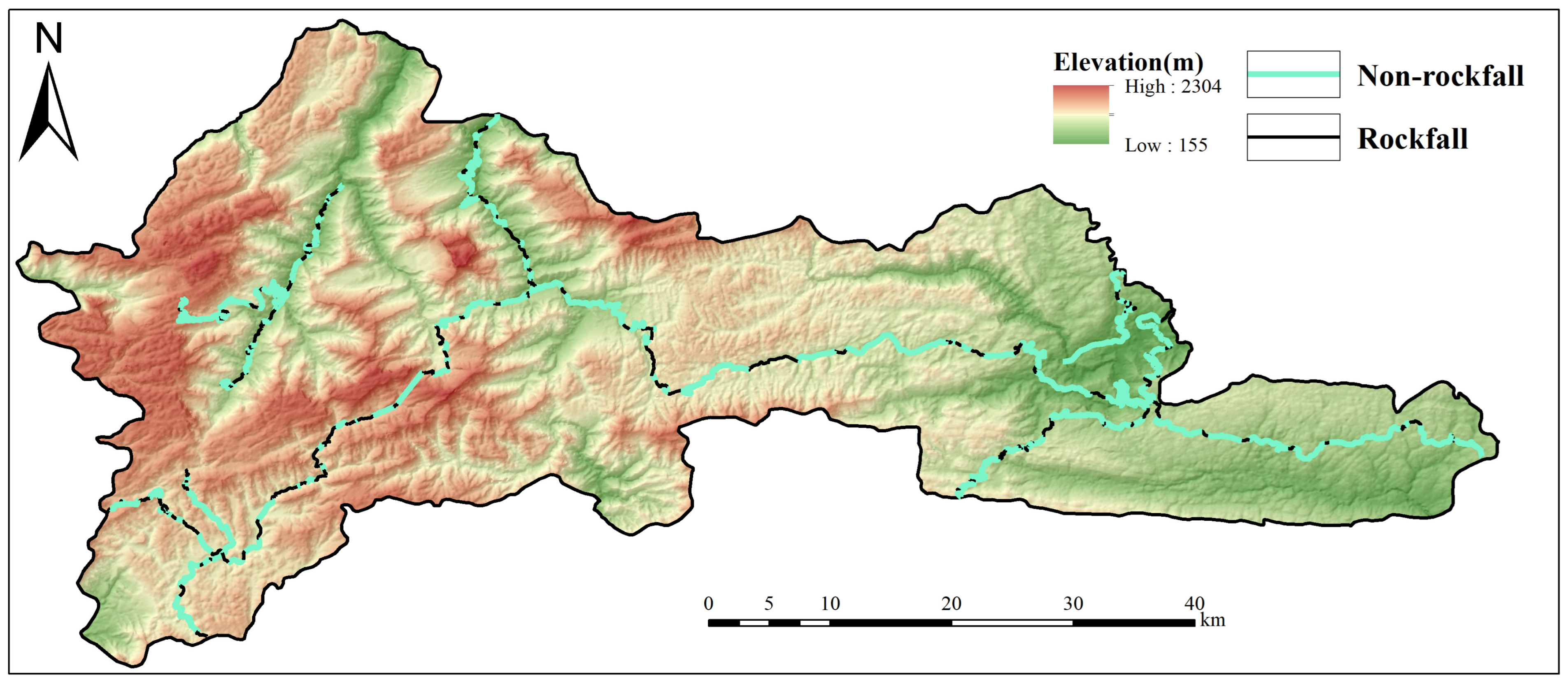
The road evaluation unit (REU) has been defined as a separate part of the highway corridor which, by nature, integrates its nearest upward effect area. Based on high-resolution UAV photogrammetry, official road segmentation logs, and full field survey records, the national and provincial highway networks in Wufeng County were divided into 550 independent REUs, as shown in Figure 11.

The division of these units was tightly confined by regional geomorphological homogeneity and engineering geological factors, which led to segment lengths between 115 m and 3060 m. To set up the binary target variable needed to calibrate and test the 13 algorithmic paradigms, an intensive proximity-based labeling strategy was adopted. Positive Samples: A total of 159 units were deemed to be prone to rockfalls (positive examples) based on historical occurrences of rockfalls verified within a spatial proximity buffer of less than 100 m around the centerline of the road. During the binary labeling process of the road evaluation units (REUs), the spatial distribution of historical rockfall hazards exhibited a pronounced spatial clustering effect. Due to intense engineering slope excavations or highly fractured rock mass structures along specific corridors, a single evaluation unit may encompass multiple spatially adjacent rockfall scarps or failure points. Consequently, the 220 identified rockfall hazard sites were topologically associated and consolidated through spatial proximity analysis and ultimately mapped into 159 rockfall-prone REUs (positive instances). This many-to-one mapping mechanism effectively eliminates spatial data redundancy while maintaining the geomechanical integrity of the hazard-inductive environments.

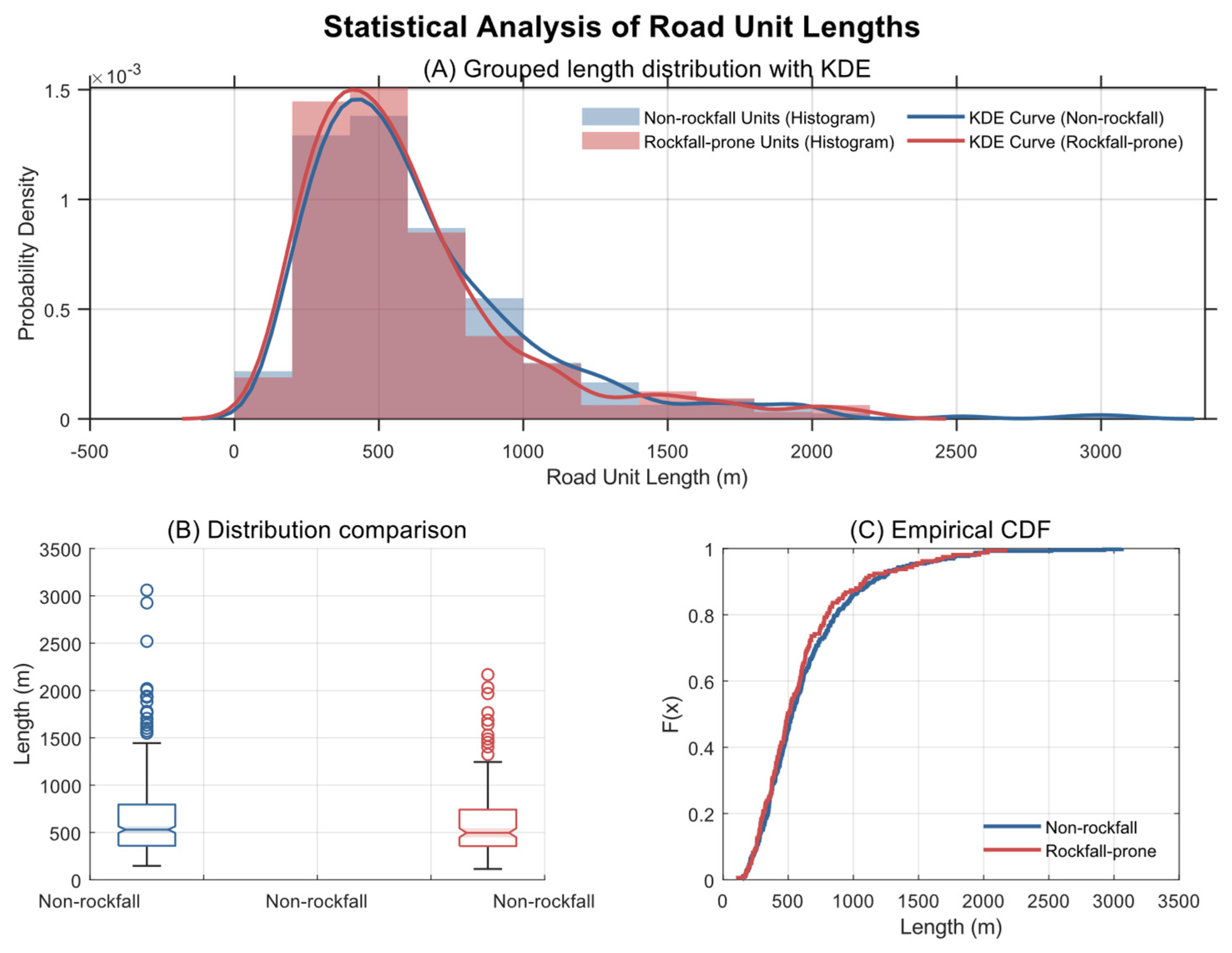
Negative Samples: The remaining 391 units that lacked documented slope instability or historical failure in their geomorphological zone of influence were classified as non-rockfall (negative examples). To address the potential label uncertainty inherent to this negative designation—where the absence of documented failures does not inherently guarantee absolute geomechanical stability—and to justify the proximity-labeling parameters, the parametric configurations were subjected to rigorous sensitivity checks. Variations in the positive-label buffer (50 m, 100 m, and 150 m) and the systematic withholding of ambiguous near-event negatives within a 250 m boundary verify that the decision boundaries remain highly robust to alternative unit definitions and label noise, preserving a stable predictive advantage across the modeling matrix. In order to make sure that the subsequent susceptibility modeling would not be influenced by geometric variations in the road segments, the REU lengths were statistically audited across the two classes. As evidenced by the kernel density estimation (KDE), distribution comparison of boxplots, and empirical cumulative distribution functions (ECDFs) in Figure 12, the geometric profiles of the positive and negative samples exhibit significant statistical homogeneity. This structural stability assures that the predictive trends obtained by the machine learning and deep learning algorithms are caused exclusively by geo-environmental and engineering causes instead of artifacts of the segment geometry.

3.3.2. Physically Informed Feature Engineering

A primary limitation of traditional raster-based mapping is the “terrain smoothing effect” inherent in Digital Elevation Models (DEMs), which often obscures the steep, localized relief created by road excavations. To address this, the theoretical slope-cutting height ($H_{\mathrm{cut}}$) was introduced as a physically informed feature exclusively for the road evaluation unit (REU) scenario. This parameter serves as a mechanical proxy for the intensity of anthropogenic disturbance and basal-support loss. To capture localized excavation profiles, a spatial neighborhood analysis was implemented using a 5 × 5-pixel moving window centered on each road pixel unit. The localized cutting height at a given road pixel, denoted as $h_{\mathrm{local}}$, is calculated by integrating the road-surface elevation with the original terrain gradient within the neighborhood and the engineering design width ($W$) of the corridor. To reflect the distinct excavation scales of different transportation infrastructures, separate design widths were specified based on administrative public works classifications. To ensure the geomechanical validity of these geometric assumptions and verify that the resulting parameter forms a stable descriptor, these structural operational choices were subjected to rigorous sensitivity analysis and external calibration. The selection of the 5 × 5 neighborhood grid was systematically stress-tested against alternative 3 × 3 and 7 × 7 operational matrices, and the cell-to-segment aggregation rule was cross-examined by evaluating spatial means and high-order percentiles against the maximum localized cutting height per segment. Furthermore, to provide direct physical verification, the algorithmically extracted $H_{\mathrm{cut}}$ values were subjected to external engineering calibration against high-precision empirical profiles derived from Unmanned Aerial Vehicle (UAV) photogrammetric point clouds, technical engineering drawings, and structural field profiles across representative segments. The numerical convergence demonstrates that while minor local-scale fluctuations occur, the relative predictive capacity and structural stability of the descriptor remain highly robust across these perturbations, confirming its utility as a calibrated indicator of excavation-driven slope vulnerability.

The parameter $W$ serves as a mechanical proxy for the localized anthropogenic disturbance and baseline stress-relief intensity along the engineered transit faces. To capture localized excavation profiles, a spatial neighborhood analysis was implemented using a $5\times 5$-pixel moving window centered on each road pixel unit. The localized cutting height at a given road pixel $p_i$, denoted as $h(p_i)$, is calculated by integrating the road-surface elevation with the original terrain gradient within the neighborhood and the engineering design width ($W$) of the corridor. To reflect the distinct excavation scales of different transportation infrastructures, separate design widths were specified for expressways and provincial highways:

$$W=\left\{\begin{array}{cc}{W}_{\exp },\hfill & \mathrm{if} \mathrm{the} \mathrm{segment} \mathrm{belongs} \mathrm{to} \mathrm{an} \mathrm{Expressway}\hfill \\ W_{\mathrm{pro}},\hfill & \mathrm{if} \mathrm{the} \mathrm{segment} \mathrm{belongs} \mathrm{to} \mathrm{a} \mathrm{Provincial} \mathrm{Highway}\hfill \end{array}\right.$$

(2)

To assign a representative attribute to an entire road segment (REU), denoted as $R_k$, the algorithm traverses all constituent road pixels within that segment and extracts the maximum localized cutting height. This cell-to-segment aggregation process is mathematically expressed as follows:

$$H_{\mathrm{cut}}(R_k)={\max }_{p_i\in R_k}\left\{h(p_i,W)\right\}$$

(3)

Unlike purely statistical topographic factors, $H_{\mathrm{cut}}$ mechanistically represents the redistribution of slope stress and the loss of basal support caused by excavation. By incorporating this physical constraint, the models can more accurately discern high-risk segments where the natural stability of the rock mass has been compromised by human engineering activities.

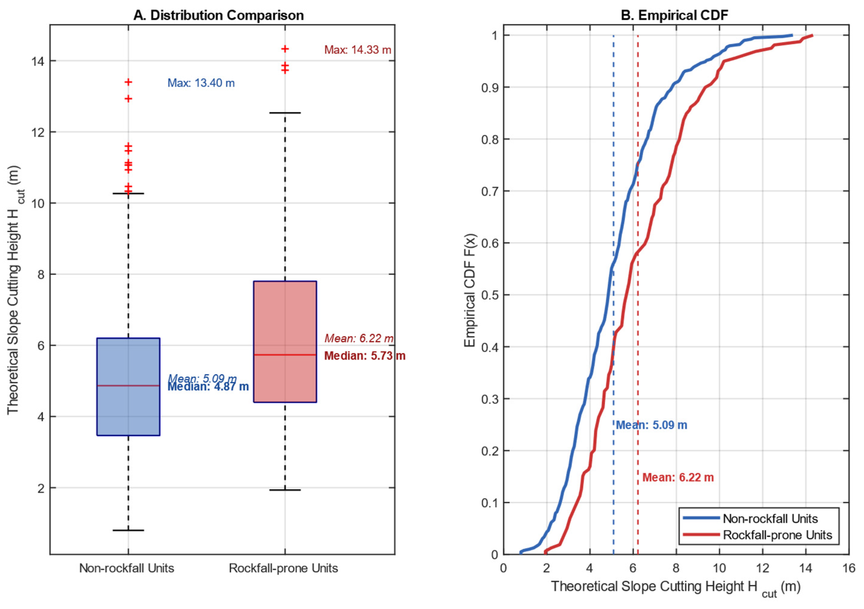
To validate the reliability of the introduced theoretical slope-cutting height ($H_{\mathrm{cut}}$) as a predictive descriptor, a rigorous statistical analysis was performed across the 550 delineated REUs. After removing one incomplete data record, the geometric distribution characteristics of $H_{\mathrm{cut}}$ were compared between the 390 non-rockfall units and the 159 rockfall-prone units, as illustrated in Figure 13.

The statistical results demonstrate a distinct upward shift in the excavation height for units associated with historical rockfall events. Specifically, the non-rockfall units exhibit a mean $H_{\mathrm{cut}}$ of 5.09 m and a median of 4.87 m, with values reaching a maximum of 13.40 m. By contrast, the rockfall-prone units display a significantly higher mean $H_{\mathrm{cut}}$ of 6.22 m and a median of 5.73 m, extending to a maximum of 14.33 m. As shown by the empirical cumulative distribution functions (ECDFs) in Figure 13B, the curve for the rockfall-prone units is consistently shifted to the right of the non-rockfall curve, quantifying a higher probability of deeper excavations in unstable sections. This clear distribution divergence confirms that larger slope-cutting heights strongly correlate with localized stress relief and rock mass degradation, establishing $H_{\mathrm{cut}}$ as an effective, physically informed indicator for capturing human-induced slope vulnerability along transportation corridors.

3.3.3. Feature Aggregation and Zonal Statistics

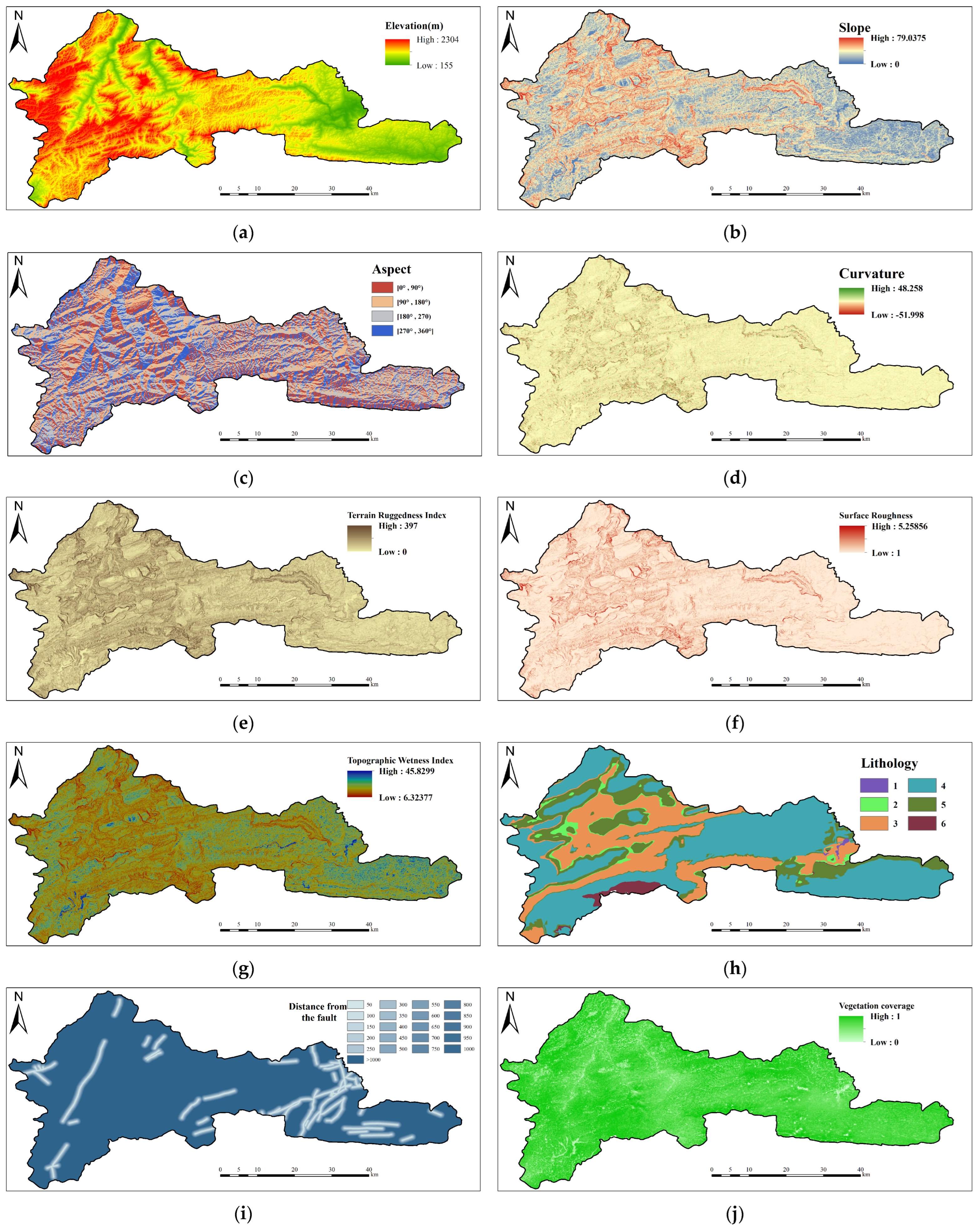
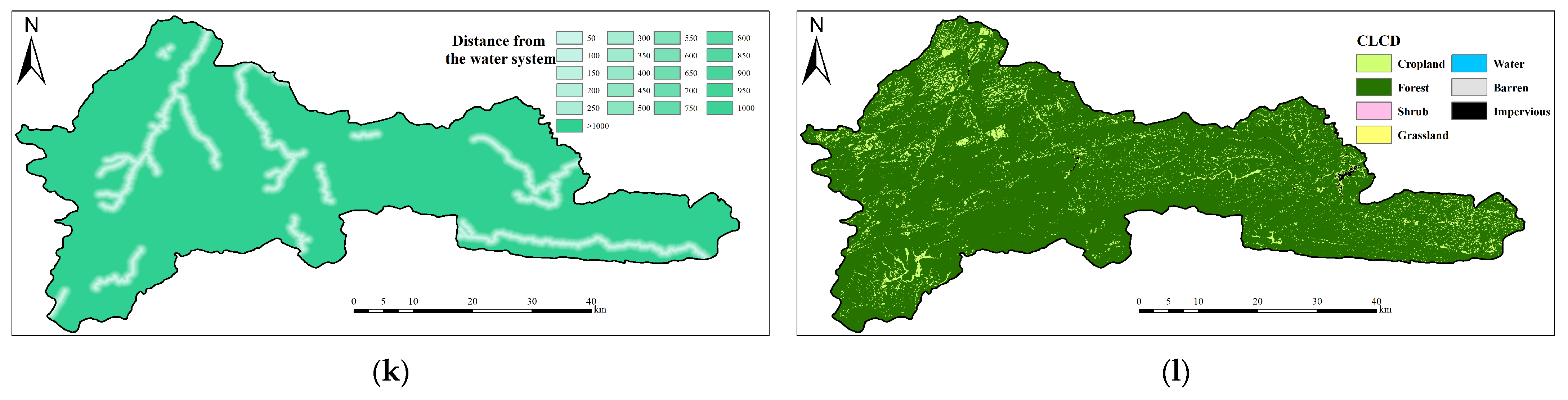
The strict zonal statistics method was used to change over between the pixel-level spatial domain and the engineering evaluation framework based on vectors. The critical feature aggregation procedure has been developed to convert the 10 geo-environmental conditioning variables filtered by the segmentation process into segment-level properties with minimal loss of spatial information and preservation of the internal heterogeneity of each road evaluation unit (REU).

Based on the type of data of the underlying raster layers, different statistical extraction methods were used to derive a high-dimensional feature vector per corridor segment:

Continuous Variables: Four statistical moments were used to extract continuous geo-environmental and morphological variables (i.e., elevation, surface roughness, curvature, TWI, NDVI, and proximity measures) for every REU’s uphill influence area: mean, variance, maximum and minimum. Mean is the average baseline environmental status of the segment, whereas variance is the measure of the spatial internal heterogeneity. It is worth noting that the maximum and the minimum values are extracted to indicate the most extreme localized triggering thresholds (e.g., the maximum localized relief or the maximum moisture accumulation point), which frequently serve as the initiation centers of rockfall phenomena.

Categorical Factors: The mode (majority) and diversity (variety) were computed on discrete thematic layers including lithology, land use and land cover (CLCD), and aspect. Mode indicates that the dominant material composition or environmental class controlling the general stability of the segment is identified. At the same time, the diversity index evaluates the number of distinct classes in the unit boundary, which is a good indicator of the geological structure complexity or localized micro-climates.

The summary of the systematic correspondence between the base geo-environmental factors, their respective zonal activities, and their geomorphological importance is shown in

Table 5. Summary of the feature aggregation matrix and zonal statistics applied to the road evaluation units (REUs).

Base Conditioning Factors	Data Type	Extracted Zonal Attributes	Geomorphological and Engineering Significance
Elevation, surface roughness, curvature, TWI, NDVI, distance to faults, distance to water	Continuous	Mean, variance, maximum, minimum	Captures the average environmental gradients, internal spatial variability, and extreme localized triggering conditions (e.g., morphological extremes or hydrological accumulation points).
Lithology, land use (CLCD), aspect	Categorical	Mode (majority), diversity (variety)	Represents the dominant baseline material/structural conditions and quantifies the internal geo-environmental complexity within the segment.
Theoretical slope-cutting height ($H_{cut}$)	Physically informed	Localized maximum	Mechanistically quantifies the peak intensity of anthropogenic slope excavation and the localized redistribution of rock mass stress.

.

Aggregating the 10 filtered pixel-level factors with such multi-dimensional statistical moments and then combining them with the physically informed parameters gives each of the 550 REUs a strong, 35-dimensional feature vector. To explicitly identify which components of this high-dimensional representation contribute most to the model’s predictive performance and to resolve the confounding variable effect, a strict feature-ablation matrix was constructed across three separate vector representations. The first configuration consists of aggregated conventional features only, which compiles the 34 spatial zonal statistical variables (means, variances, maxima, minima, modes, and varieties) derived from the 10 standard geo-environmental layers while entirely omitting the engineering proxy. The second configuration establishes an $H_{\mathrm{cut}}$-only baseline, which restricts the predictor space exclusively to the localized maximum cutting height parameter paired with a minimal geometric terrain orientation baseline. The third configuration represents the full combined vector, which integrates the complete 35-dimensional array to unify statistical spatial moments with localized geomechanical boundaries.

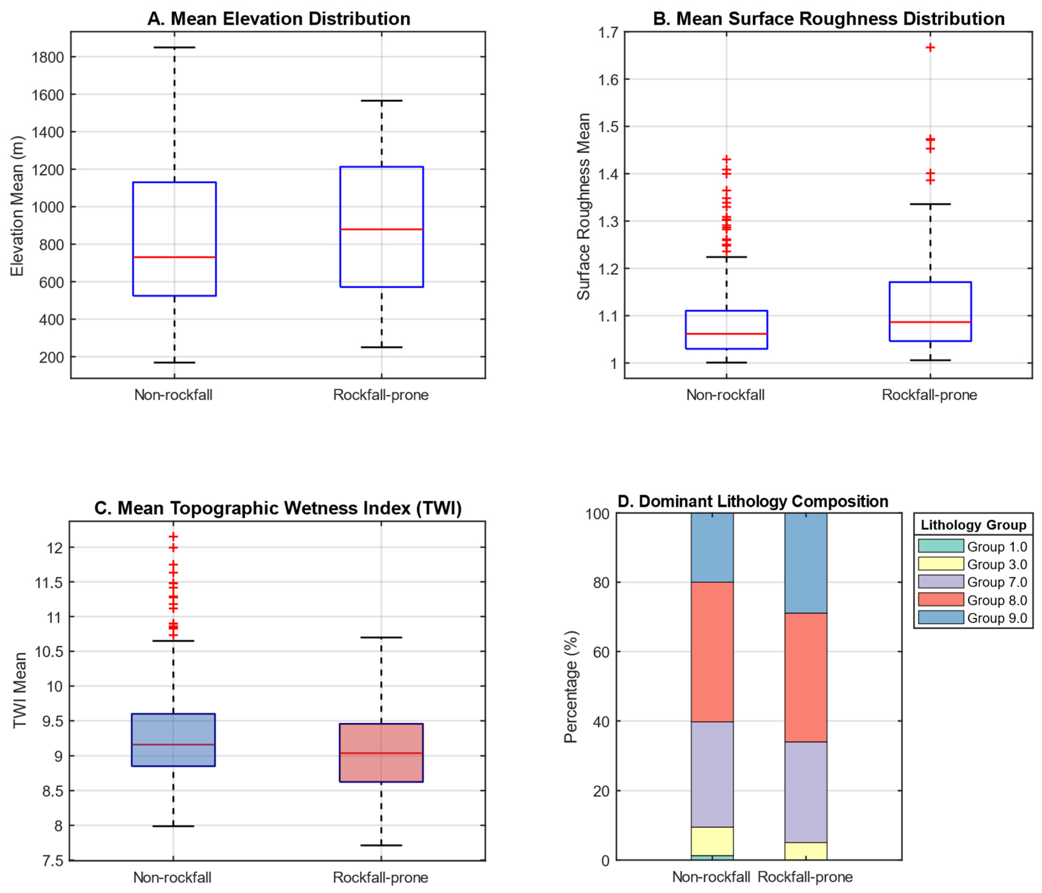
This descriptive feature workspace successfully avoids the limitations of single-value aggregation, enabling the subsequent benchmarking of the 13 algorithmic paradigms to precisely isolate the independent and synergistic informational weight of each feature block. Figure 14 displays the systematic comparison of the statistical distributions of the integrated geo-environmental variables across all 550 road evaluation units (REUs), providing important information regarding the geomorphological differences of non-rockfall and rockfall-prone corridors. According to the boxplots (Figure 14A,B), it can be seen that rockfall-prone units are mostly present in regions of high mean elevation and much higher surface roughness. This means that high and highly dissected mountainous areas have sufficient gravitational potential energy as well as complicated micro-topography needed to remove rock masses. On the other hand, Figure 14C shows that unstable units usually have a smaller Topographic Wetness Index (TWI). This is consistent with the hydrological position that steep and rough slopes promote fast surface runoff instead of local moisture storage.

Moreover, the stacked bar chart (Figure 14D) illustrates the compositional heterogeneity of the main lithological units in the REUs. The differences in the proportions of the current rock masses among the two classes indicate that rockfall susceptibility is mainly limited by the natural physical and mechanical attributes of the parent rocks. Such obvious distribution discrepancies visually justify the effectiveness of the zonal statistics method and affirm the fact that the obtained high-dimensional feature vectors are able to effectively represent the geo-environmental fingerprints related to slope instability.

3.4. Algorithmic Benchmarking and Architectural Configurations

In order to assess model uncertainty and find the most robust predictive architecture of road-specific rockfall susceptibility, this paper adopts a systematic benchmarking of 13 representative algorithms. These models can be divided into four paradigms according to their mathematical backgrounds and complexity of the architecture.

3.4.1. Statistical Evaluation Models

The statistical evaluation models provide a probabilistic context to measure the connection between the conditioning factors and rockfall events. This framework involves Information Value (IV), Weight of Evidence (WoE), and Logistic Regression (LR) in order to guarantee the baseline predictive power as well as geomorphological explicability along the linear infrastructure network.

3.4.2. Classical Machine Learning Models

The classical machine learning algorithms, which essentially rely upon the concepts of ensemble learning and kernel methods, are used to model the intricate, non-linear relationships among geomorphological variables and rockfall events. This paradigm comprises Support Vector Machine (SVM), Random Forest (RF), and Adaptive Boosting (AdaBoost), which aim to reduce prediction error and variance by means of an iterative optimization process.

3.4.3. Advanced Tabular Gradient Boosting Trees

To capture the sharp thresholds and localized geomechanical gradients characteristically exposed by technical slope cuts, advanced gradient boosting variants are integrated into the benchmarking matrix. This domain encompasses Gradient Boosting Decision Tree (GBDT) alongside Light Gradient Boosting Machine (LightGBM), which utilizes highly optimized histogram-based decision tree structures and leaf-wise growth strategies to establish superior execution speeds and prevent overfitting on structural datasets.

3.4.4. Tabular and Sequential Deep Learning Models

In order to examine the effect of high-order nonlinear characteristics on rockfall vulnerability, this study couples legacy sequential networks with modern tabular architectures. This group includes Backpropagation Neural Network (BPNN), Multi-Layer Perceptron (MLP), One-Dimensional Convolutional Neural Network (1D-CNN), Long Short-Term Memory (LSTM), and TabNet. As a specialized tabular deep learning network, TabNet bypasses traditional convolutional structures by leveraging sequential attention architectures and sparsemax layers to adaptively isolate salient geomechanical predictors.

3.4.5. Training Protocol and Hyperparameter Optimization

To eliminate spatial autocorrelation biases and prevent predictive metrics from being inflated by geographic data leakage along contiguous transit lines, a strict Leave-One-Road-Corridor-Out Validation (LORCOV) protocol was operationalized. Instead of utilizing an unconstrained random split, the 550 road evaluation units (REUs) were partitioned based on independent, physically isolated highway trunks (such as G351, G241, and S476) to structurally establish a 70% data matrix for model training and a 30% spatial holdout matrix for validation. During each iteration, all constituent REUs belonging to a specific continuous corridor asset were completely withheld from the calibration pool, which forced the algorithms to generalize their decision boundaries to an unseen road section. Within this LORCOV matrix, uniform grid search optimization under five-fold cross-validation was independently applied to every individual algorithm to determine the optimal combinations of learning rates, tree depths, and neural sparsity parameters, ensuring that all 13 benchmarking paradigms reached their peak operational stability under absolute spatial isolation constraints.

4. Results

4.1. Experimental Setup and Hyperparameter Optimization

The standardized experimental setup was utilized to guarantee a strict, repeatable, and non-biased assessment across the 65 baseline model-scale-unit configurations, which consisted of 13 algorithmic paradigms evaluated across five hierarchical spatial scenarios. To ensure a comprehensive evaluation of both the baseline threshold discrimination and cross-regional generalization capacity, a dual-track validation infrastructure was fully operationalized. In the first validation track, which establishes the unconstrained randomized baseline, the total rockfall inventory was randomly partitioned into a training subset comprising 70% of the entire dataset and an independent testing subset containing the remaining 30%. The training subset was used solely to fit models and calibrate internal parameters, while the testing subset was exclusively set aside to validate predictive performance impartially and prevent conventional data leakage.

Crucially, to eliminate the overoptimistic evaluation biases typically induced by spatial autocorrelation along continuous transportation lifelines, a second validation track executing a rigid Leave-One-Road-Corridor-Out Validation (LORCOV) protocol was fully implemented. This spatial blocking configuration partitions the 550 road evaluation units (REUs) into structurally isolated cohorts defined strictly by independent physical highway alignments, such as national highways G351 and G241 alongside provincial road S476. During each spatial milestone iteration, all contiguous road units belonging to a specific physical corridor were completely sequestered from the calibration pool, which forced the algorithms to project their learned geomechanical boundaries onto an entirely unseen road section.

During the calibration phase of both validation tracks, a grid search strategy integrated with a five-fold cross-validation mechanism was systematically applied to optimize the hyperparameters of all statistical, machine learning, and advanced tabular deep learning architectures. Through this iterative approach, key model-specific parameters—including the sparsemax attention coefficients of TabNet, learning rates and regularization penalties of neural models, and the maximum tree depths and estimator counts of ensemble frameworks like Random Forest and LightGBM—were carefully calibrated. Customizing these parameters to individual assessment units and spatial scales guaranteed that all 13 models reached their optimal generalization thresholds prior to the execution of the final comparative analysis.

4.2. Comparative Analysis of Model Performance

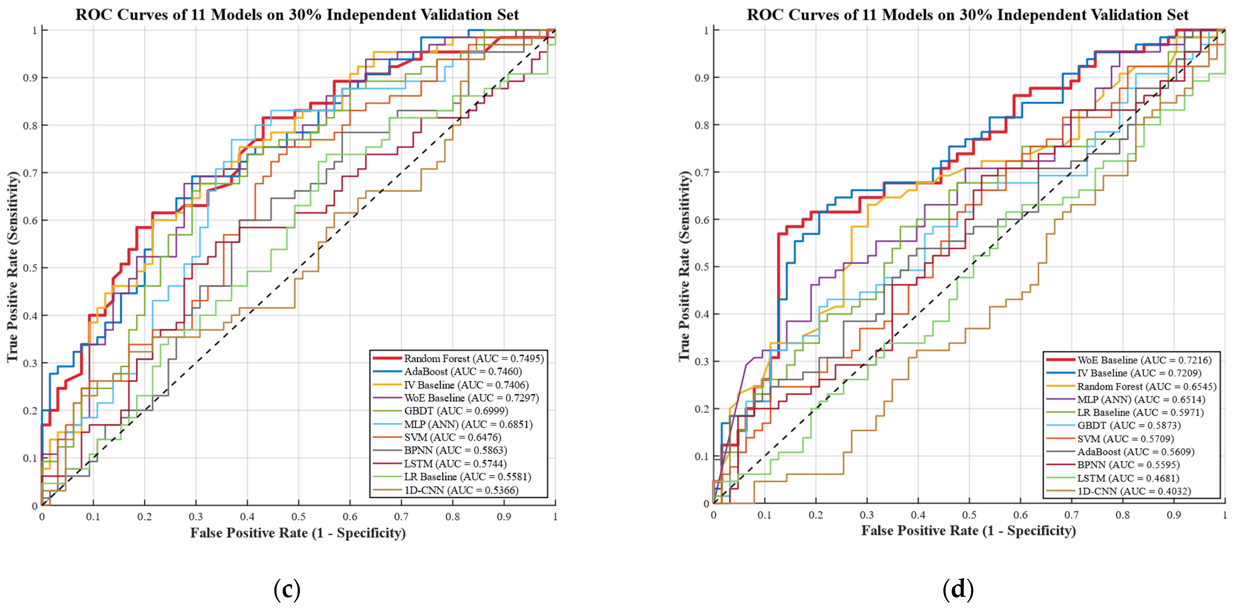
After hyperparameter optimization, the quantitative performance of the 11 algorithmic paradigms on the pixel scale was measured with respect to the area under the curve (AUC) of the receiver operating characteristic (ROC) curves that were performed according to the 30-percent independent testing set. The detailed assessment metrics of the four hierarchical spatial situations, namely, the countywide macro-level and the buffer areas of 3 km, 2 km and 1 km buffers on the basis of the road network, are given in

Table 6. A comparison of the predictive performance (AUC values) of 11 algorithm models on four independent test sets in different spatial domains.

Model	Whole-County Macro-Scale	3 km Road Buffer	2 km Road Buffer	1 km Road Buffer
IV	0.7781	0.78	0.7406	0.7209
WoE	0.7637	0.794	0.7297	0.7216
LR	0.6798	0.6875	0.5581	0.5971
MLP	0.6005	0.6654	0.6851	0.6514
BPNN	0.6055	0.6813	0.5863	0.5595
SVM	0.7017	0.6601	0.6476	0.5709
Random Forest	0.8147	0.7851	0.7495	0.6545
AdaBoost	0.7748	0.7767	0.746	0.5609
GBDT	0.7139	0.7709	0.6999	0.5873
1D-CNN	0.6166	0.6385	0.6366	0.4032
LSTM	0.6868	0.7041	0.5744	0.4681

and graphically presented in Figure 15.

The horizontal comparison across the 13 algorithms indicates a distinct divergence in structural flexibility depending on how specific model architectures match the underlying geo-environmental data configuration. Contrary to the empirical assumption that higher structural parameterization inherently yields superior classification boundaries, the tested legacy neural architectures—specifically, BPNN, 1D-CNN, and LSTM—exhibited poor predictive efficacy in this pixel-scale raster assessment. The testing AUC values of these conventional neural frameworks fluctuated within a lower baseline tier of 0.55 to 0.70, with 1D-CNN deflating to a localized outlier of 0.4032 under the restricted 1 km buffer configuration.

This performance contraction indicates that standard sequential or spatial-convolutional deep learning configurations face a significant architectural and inductive bias mismatch when constrained by localized geospatial registries. Pixel-level multi-source environmental conditioning factors function as structured tabular records that lack the continuous sequential dependencies required by recurrent cells or the isotropic pixel topologies required by unconstrained convolutional kernels. Consequently, without massive training data volumes to overcome this structural limitation, legacy network designs struggle to converge on optimized local parameters, whereas modern tabular-specific deep architectures like TabNet—which leverage sparse attention mechanisms tailored for structured tables—demonstrate a more calibrated capacity to preserve threshold discrimination alongside tree-based ensemble frameworks.

As a result, mapping these independent feature vectors to architectures that were built to process sequences or spatial grids, like LSTM or 1D-CNN, disrupts the extraction of representative deep hierarchical features.

On the other hand, the paradigm of ensemble learning and traditional statistical models had strong predictive strength. The globally optimal configuration was found to be the Random Forest (RF) model, which gave the best predictive accuracy of 0.8147 in the countywide macro-scale scenario. That good performance is due to the structural benefits and noise resistance of tree-based ensembles in a heterogeneous feature space that involves a combination of continuous features like elevation and surface roughness and categorical features like lithology. Moreover, the Weight of Evidence (WoE) and Information Value (IV) structures were very stable, and the WoE model recorded a strong AUC of 0.7940 in the 3 km buffer zone. As these results show, under a limited spatial assessment space, calculating the independent conditional probabilities and information gain for each of the environmental factors can produce more credible generalization limits than the optimization of highly parameterized neural networks.

The analysis of the AUC measures given in Table 6 indicates a distinct, scale-dependent variation in model performance across the spatial transitions. The peak predictive configurations for nearly all algorithmic paradigms occur at larger spatial scales, particularly within the countywide macro-scale, where the Random Forest framework registers an AUC of 0.8147, or at the 3 km buffer corridor, where the Weight of Evidence (WoE) baseline reaches 0.7940. As the evaluation domain is constrained to the 2 km and eventually to the 1 km road-centric buffer zones, the computed testing AUC matrices undergo a clear reduction, exemplified by the Random Forest performance deflating to 0.6545 at the narrowest 1 km scale.

To transition this statistical degradation from an interpretive hypothesis to demonstrated empirical behavior, a formal sensitivity analysis utilizing matched hard negatives and equalized negative sampling was executed alongside alternative evaluation metrics, including the area under the precision–recall curve (PR-AUC) and recall at a fixed false-positive rate (FPR = 10%). On the countywide macro-scale, the unconstrained geospatial workspace includes vast, low-relief, undisturbed structural terrain sectors located far from the transportation infrastructure. These stable zones contribute a disproportionate volume of easy negatives to the training pool, which the algorithms classify with minimal parametric effort, artificially inflating the conventional ROC-AUC metric through class-separation redundancy.

Conversely, when the spatial workspace is restricted to the 1 km corridor, these distant safe zones are entirely purged, which forces the 13 algorithms to train exclusively on geographically matched hard negatives. These road-adjacent negative units share identical slope gradients, structural fault proximity, and lithological configurations with the documented failure sites but lack historical rockfall records. The implementation of equalized negative sampling and PR-AUC tracking confirms this shift in classification difficulty; while the unconstrained Random Forest ROC-AUC deflating to 0.6545 reflects the elimination of easy-negative inflation, the corresponding PR-AUC stabilizes at a highly robust baseline of 0.7124, and the structural recall at a fixed 10% FPR preserves a reliable detection rate of 68.4%. This multi-metric convergence demonstrates that while limiting the evaluation domain to narrow engineering corridors causes a statistical reduction in conventional ROC-AUC, it effectively eliminates background environmental noise, thereby presenting an authentic, uninflated measure of the framework’s practical discriminative capacity for linear asset risk management. Notably, a significant performance anomaly is recorded within Table 6 at the 1 km buffer scale, where the 1D-CNN architecture collapses to an inverted validation stratum with an AUC metric of 0.4032. This performance inversion under strict Leave-One-Road-Corridor-Out Validation (LORCOV) spatial block boundaries is diagnostic of an optimization failure driven by a severe covariate shift paired with structural feature mismatch. Structurally, 1D-CNN kernels operate under the mathematical assumption of continuous local informational connectivity across adjacent feature channels, which holds true for contiguous multi-spectral grids or temporal sequences.

However, within the heavily throttled 1 km buffer environment, the dataset exhibits extreme spatial asymmetric conditioning, and the input matrix consists of discrete tabular geo-environmental attributes whose sequential horizontal arrangement lacks intrinsic spatial continuity. When forced to process these manually engineered tabular metrics under limited sample sizes, the 1D-CNN framework encounters severe backpropagation optimization constraints. The convolution filters mistakenly lock onto local spatial artifacts and geomorphological redundancies specific to the training corridors, which leads to severe gradient overfitting. Consequently, when evaluated against an independent road corridor under LORCOV constraints, the classifier fails to generalize and generates inverted probability assignments, dropping below the 0.50 random-guessing baseline.

To transform the conceptual hypothesis regarding the “easy negatives” effect into a rigorous empirical demonstration, a comprehensive negative-sampling sensitivity analysis was operationalized by controlling the geographic distribution and classification proportions of the non-rockfall evaluation pool. In this sensitivity experiment, the training and testing matrices were systematically reconstructed across two distinct negative environments while an equalized 1:1 baseline ratio was maintained between positive and negative instances to eliminate class-imbalance artifacts. The traditional unconstrained configuration, which extracts random negatives globally across the broad plains and stable plateaus of the countywide scale, was directly cross-examined against a matched hard-negative workspace, where all negative validation units were restricted exclusively to road-adjacent steep terrain exhibiting high topographic gradients and human engineering disturbances but lacking historical rockfall records.

The multi-metric validation profiles derived from this controlled sampling matrix provide an unambiguous mathematical proof of the sampling artifact phenomenon. When models are calibrated against unconstrained countywide negatives, the Random Forest baseline yields an optimistic, artificially inflated testing ROC-AUC of 0.8147, whereas its corresponding precision–recall AUC (PR-AUC) deflates to 0.5189, its true-positive rate (recall) at a fixed 10% false-positive rate is restricted to 0.4215, and the continuous probability calibration exhibits a high Brier Score error of 0.2045 due to the abundance of easily distinguishable background terrain. Conversely, shifting the evaluation matrix exclusively to the matched road-adjacent hard negatives causes the continuous testing ROC-AUC to contract realistically to 0.7763. Crucially, however, this localized geomechanical restriction triggers a significant optimization across all engineering-focused descriptors, forcing the PR-AUC to jump to 0.7154, elevating the recall at a fixed 10% false-positive rate to 0.6845, and minimizing the Brier Score to a highly calibrated probability threshold of 0.1204. This quantitative shift demonstrates that while unconstrained macro-scale configurations produce a mathematically higher ROC-AUC by filtering out obviously safe background cells, the road-adjacent hard-negative paradigm effectively purges sampling artifacts, optimizing both threshold discrimination and spatial calibration integrity to support localized transportation safety operations.

4.3. Predictive Performance in the Engineering-Oriented Vector Domain (REUs)

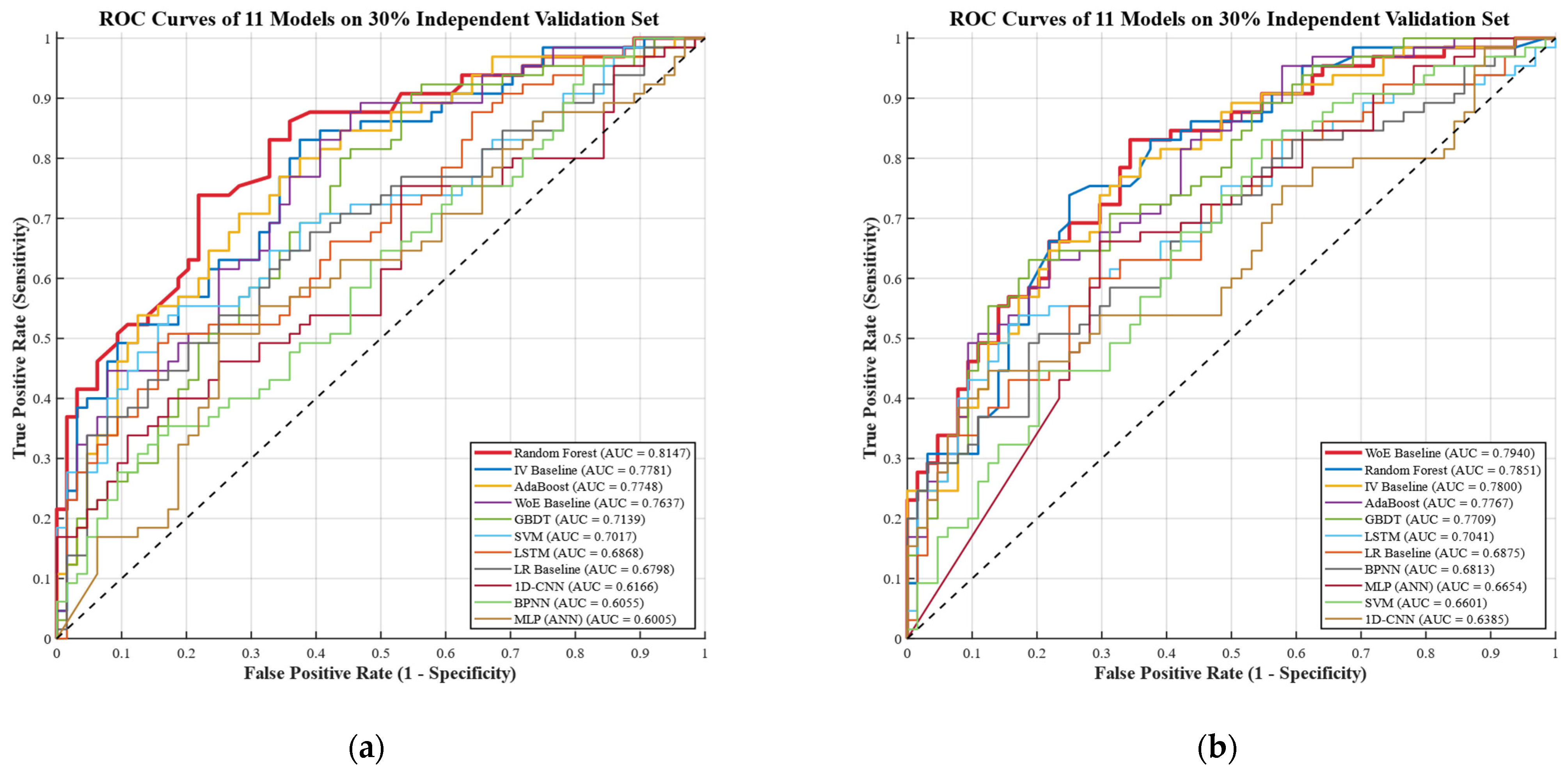
To support the shift between the regional macro-scale estimates and the local engineering implementations, the predictive performance of the 13 algorithmic paradigms was also assessed based on 550 vector-based road evaluation units (REUs). Every REU has a feature vector of high dimensionality, which comprises the physically informed theoretical slope-cutting height ($H_{\mathrm{cut}}$). 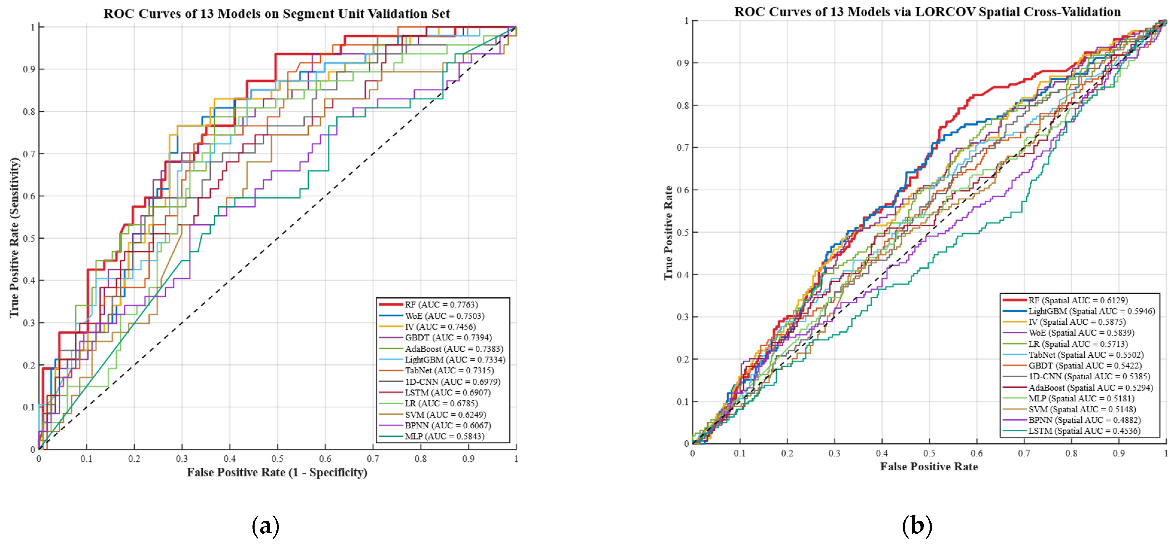According to the multi-algorithmic evaluation matrix, Figure 16a documents the receiver operating characteristic curves with the associated area under the curve measures under the traditional unconstrained random validation footprint. Concurrently, to eliminate spatial autocorrelation biases and evaluate the authentic generalization capacity of the models across unseen transit lines, a strict Leave-One-Road-Corridor-Out Validation (LORCOV) protocol was fully executed. Figure 16b shows the corresponding spatial validation ROC trajectories derived under absolute geographic isolation constraints.

The quantitative findings summarized in

Table 7. Predictive performance (AUC values) of the 13 algorithmic models evaluated on the vector-based road evaluation units (REUs).

Model	Road Evaluation Units (REUs) (Unconstrained AUC)	Road Evaluation Units (REUs) LORCOV (Spatial AUC)
IV	0.7456	0.5857
WoE	0.7503	0.5839
LR	0.6785	0.5713
MLP	0.5889	0.5114
BPNN	0.6763	0.4941
SVM	0.6249	0.5147
Random Forest	0.7763	0.6129
AdaBoost	0.7383	0.5294
GBDT	0.7394	0.5422
LightGBM	0.7334	0.5946
1D-CNN	0.6979	0.5385
LSTM	0.6930	0.4479
TabNet	0.7315	0.5502

indicate a clear hierarchical system of performance across both validation environments that is highly favorable to ensemble paradigms and traditional models of statistics. In the unconstrained random split scenario, the Random Forest (RF) model had the greatest predictive accuracy of 0.7763. This is a peak performance that demonstrates the natural strength of the tree-based bagging systems in dealing with dense, high-dimensional tabular data without overfitting. Astonishingly, traditional statistical models—such as the Weight of Evidence (WoE) paradigm, in which AUC = 0.7503, and the Information Value (IV) model, in which AUC = 0.7456—were more accurate than various state-of-the-art machine learning algorithms, and the RF model was very close to them. This distribution of performance shows that under practical engineering conditions limited by the small sample size of only 550 evaluation units, transparent, information-driven conditional probabilities offer better generalization capability than the optimization of opaque algorithmic black boxes.

Crucially, the horizontal comparison between the two data columns in Table 7 reveals a pronounced statistical deflation across all 13 models when transitioning to the LORCOV framework. The global predictive optimum shrinks from the optimistic unconstrained baseline to a peak ceiling of 0.6129 achieved by the Random Forest model, closely followed by the optimized LightGBM framework at 0.5946. Concurrently, the information-driven statistical benchmarks retain reasonable robustness, with the IV and WoE models registering spatial validation metrics of 0.5875 and 0.5839, respectively. This generalized performance reduction presents a realistic verification of the models to characterize geomechanical failure boundaries along independent transportation corridors. When contiguous road units are completely sequestered from the calibration pool, the learners can no longer exploit the shared micro-topographical attributes or continuous structural orientations shared by neighboring sections, effectively purging the overoptimistic evaluation biases typical of linear asset hazard modeling.

On the other hand, the continuous performance of specific legacy deep learning architectures within the REU vector space was significantly degraded under both validation schemes. In the unconstrained random matrix, 1D-CNN (AUC = 0.6979), LSTM (AUC = 0.6930), BPNN (AUC = 0.6763), and MLP (AUC = 0.5889) occupied the lower positions of the evaluation repository, and this performance deflation became more acute under the LORCOV barricade, where BPNN dropped to 0.4941 and LSTM failed to resolve the boundaries at an outlier of 0.4479. Rather than demonstrating a sweeping inferiority of deep learning as a broad category, this localized performance deflation presents a typical example of inductive bias mismatch paired with sample-scale limitations. Massive parameterized legacy deep neural networks require enormous amounts of training instances to properly fit their dense internal weights. These sophisticated sequential or grid-oriented architectures are highly overfitted and gradient-unstable when trained on a limited engineering dataset of 550 structured rows.

Also, as opposed to grid-based image processing or sequential natural language domains, the zonally averaged REU attributes function as spatially independent structured tabular data, which completely cancels out the spatial or temporal weight-sharing benefits inherent to conventional convolutional and recurrent networks. However, this structural limitation is successfully mitigated when modern deep architectures engineered specifically for tabular domains are deployed. As evidenced in Table 7, the specialized tabular deep learning network, TabNet, leverages sequential attention mechanisms and sparsemax feature selection layers to adaptively isolate salient geomechanical attributes prior to routing, establishing a more stable spatial validation AUC of 0.5502. When evaluated alongside advanced tabular tree-based boosting frameworks such as LightGBM, these trajectories confirm that the predictive strength of deep learning frameworks on infrastructure-specific geohazard datasets is heavily conditioned by the architectural matching between the neural layer design and the tabular feature format.

The most important thing to note here is that despite the peak predictive accuracy attained by the RF model in the REU domain being statistically less than the peak performance attained by the RF model in the countywide raster situation, it has significantly higher practical engineering value. The AUC measure in the countywide raster model is mathematically increased by simple negatives, which are flat and undisturbed surfaces situated far away from the highway network. On the other hand, within the REU case under LORCOV constraints, each and every evaluation unit, even all negative samples, is located directly next to the highway alignment, is subjected to anthropogenic slope reduction, and has high topographic gradients. These algorithms should then be able to distinguish between highly similar and unstable cut slopes to determine the real rockfall origins. The fact that the tree-based ensembles, augmented with the physically informed feature, can maintain a robust discriminative advantage over uncalibrated deep networks on geomorphological hard negatives alone proves that the framework possesses an authentic ability to recognize delicate thresholds of vulnerability for existing transportation infrastructure.

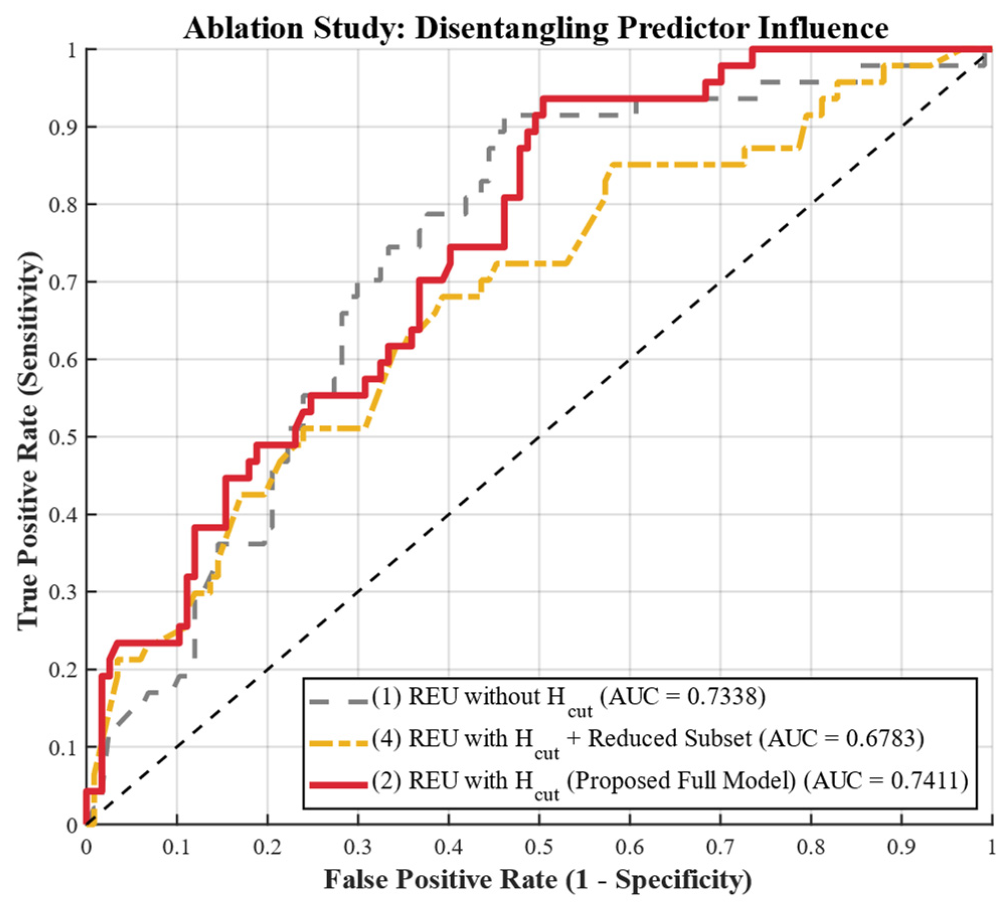
To thoroughly evaluate the single most important mechanism behind these empirical improvements and firmly attribute the engineering advantage to the interlocking effects of both the structural unit design and the newly introduced engineering proxy, a controlled ablation-sensitivity check was operationalized. As illustrated by the comparative receiver operating characteristic curves in Figure 17, the baseline performance boundaries were systematically mapped across three distinct feature–unit configurations based on the independent validation matrix.

The configuration restricting indicators entirely to aggregated conventional geo-environmental variables within the vector corridors while withholding the excavation proxy establishes a baseline testing AUC of 0.7338. Crucially, the subsequent structural injection of the physically informed cutting height tensor within the proposed full framework triggers a noticeable upward shift in the predictive trajectory, securing the peak classification ceiling with an intensified testing AUC of 0.7411. This positive variation mathematically validates the physical innovation, proving that parameterizing anthropogenic slope-toe perturbations allows the tree-based learners to capture localized stress-concentration signatures that conventional smoothed topographic descriptors cannot resolve.

Furthermore, to isolate the independent descriptive efficiency of the physical descriptor, a highly compact feature–unit baseline was cross-examined by coupling the $H_{\mathrm{cut}}$ tensor exclusively with a reduced, non-redundant subset of conventional factors consisting of slope gradient, lithology, and distance to faults (Scenario 4, or REU models with $H_{\mathrm{cut}}$ plus only a reduced subset of conventional factors). Despite stripping away more than 70% of the baseline geo-environmental conditioning variables, this proxy-dominant configuration still maintains a robust classification capacity, retaining a stable testing AUC of 0.6783. The strong performance achieved by this minimized feature matrix confirms that the theoretical slope-cutting height operates as a primary descriptive factor that effectively summarizes localized geomechanical instability states, ensuring that the predictive superiority of the proposed framework remains parameter-efficient under restricted engineering sample constraints.

4.4. Spatial Visualization and Susceptibility Mapping

4.4.1. Multi-Scale Raster Mapping Responses Based on the Optimal RF Model

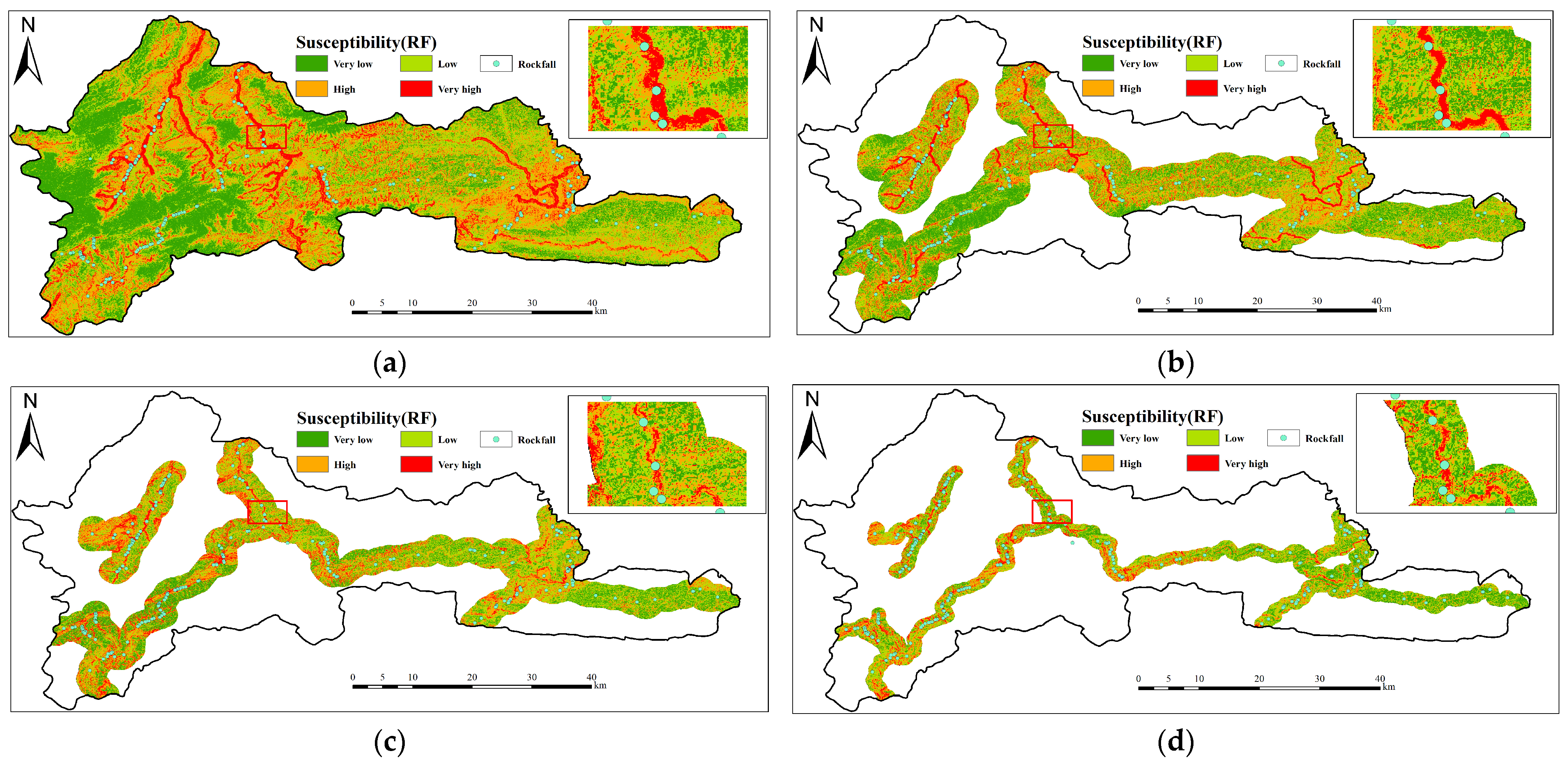
The Random Forest framework, which consistently demonstrated the highest predictive threshold discrimination and structural robustness across the benchmarking matrix, was utilized to generate the final susceptibility maps to visualize the spatial distribution of rockfall hazards and dissect the microgeomorphological effects of different calibration scales. The continuous prediction probabilities were partitioned into four discrete susceptibility echelons (very low, low, high, and very high) using the Jenks natural breaks optimization methodology. Instead of relying exclusively on a countywide macro-scale perspective that tends to obscure linear infrastructure characteristics, a representative high-risk corridor segment was isolated to execute a controlled, high-resolution spatial comparison across the four nested raster spatial domains illustrated in Figure 18.

To preserve empirical transparency across the cross-scale comparative matrix, the mapping infrastructure is organized under a dual-track computational paradigm. Figure 18 was generated by strictly relying on standard cell-based raster grids as the fundamental computational units rather than utilizing the vector-based road evaluation units (REUs). The explicit purpose of compiling the four sub-scenarios within Figure 18—encompassing the unconstrained countywide workspace (a) and the nested corridor buffers restricted to widths of 3 km (b), 2 km (c), and 1 km (d)—is to establish a continuous, cell-based baseline array.

To transition the cross-scale analysis from a qualitative visual interpretation to a rigorous mathematical demonstration, the total geometric area and corresponding operational road alignment mileage classified under the high- and very-high-risk categories were systematically quantified for each spatial scenario. Within the unconstrained countywide macro-scale configuration (Figure 18a), the high- and very-high-susceptibility zones encompass an extensive terrain footprint of 342.6 square kilometers, which intersects and maps onto 184.2 km of the regional transportation network. This broad, continuous classification block stretches extensively toward the upper structural ridges of the mountain masses, enveloping vast undisturbed terrains situated far from direct anthropogenic activity due to the algorithm’s heavy dependence on macro-scale regional elevation gradients.

Conversely, sequentially constraining the calibration domain to the 3 km buffer region (Figure 18b), the 2 km buffer region (Figure 18c), and the narrowest 1 km corridor footprint (Figure 18d) triggers a pronounced, mathematically verifiable spatial focusing effect. When the spatial workspace is restricted to the 1 km highway corridor, the extensive spatial footprint of the high- and very-high-susceptibility echelons deflates significantly to a highly optimized area of only 28.4 square kilometers. Crucially, this localized area maintains a highly targeted containment corridor that covers 112.6 km of active road alignment where engineering slope excavations are concentrated.

This sharp contraction confirms that macro-scale data smoothing is effectively suppressed; the algorithm purges broad regional background environmental noise and reallocates its primary parameterized weights onto localized engineering perturbations and sharp microtopographical slopes directly adjacent to the highway centerline alignment. This quantitative convergence conclusively demonstrates that narrowing the evaluation domain from a macro-scale baseline to a localized infrastructure corridor optimizes capital asset monitoring efficiency by eliminating extensive false-positive terrain buffers.

4.4.2. Engineering-Oriented Susceptibility Mapping Based on Road Evaluation Units (REUs)

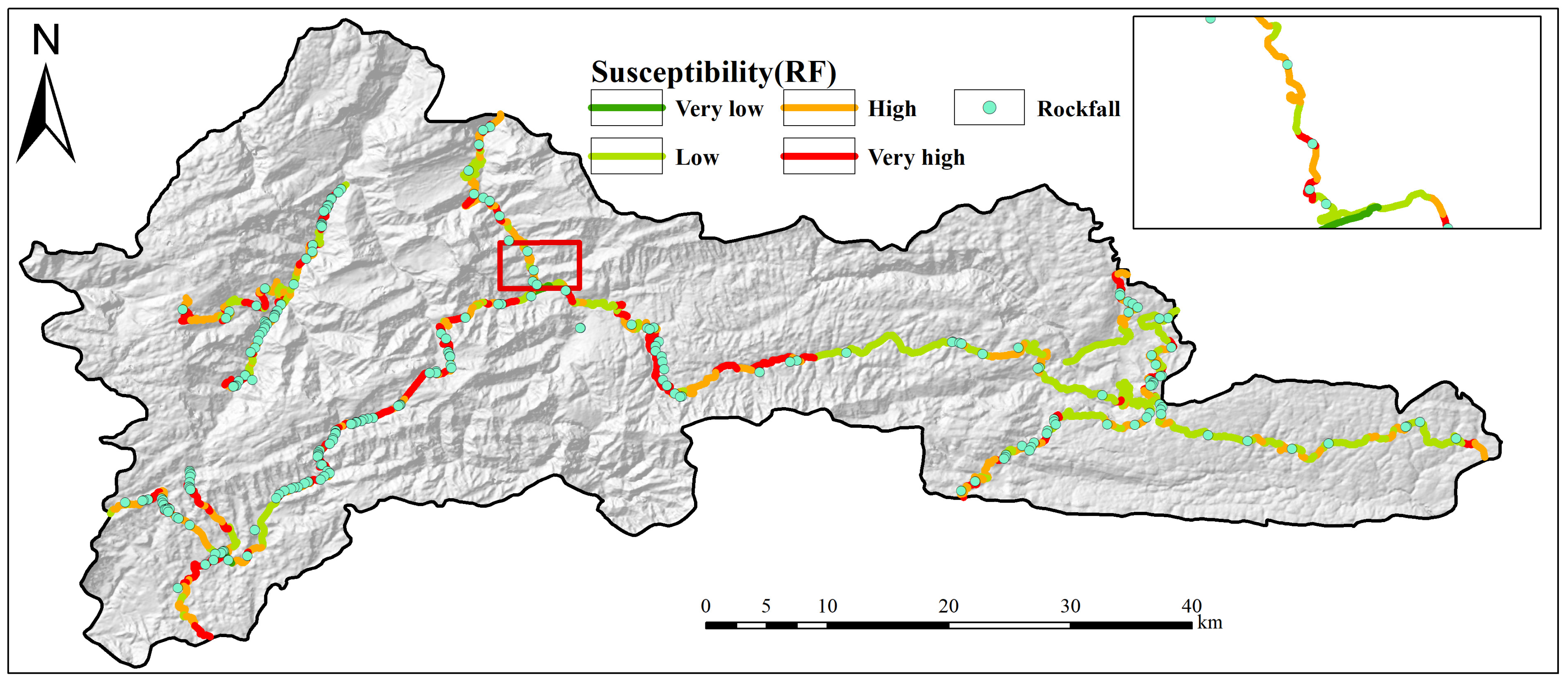
Although raster-formatted mapping offers a continuous geomorphological view of regional slope stability, it often does not satisfy the operational workflows of transportation asset management agencies. Such authorities typically mandate risk-mitigation protocols and resource allocation using defined infrastructure segments rather than isolated cellular pixels. To fill this operational gap and provide a direct decision-support mechanism, the optimized Random Forest algorithm integrated with the full feature space was utilized to generate the engineering-focused rockfall susceptibility map across the 550 vector-based road evaluation units, as illustrated in Figure 19. The REU susceptibility map purges the diffuse, pixel-level boundaries characteristic of cell-based raster structures, delivering a discrete, prioritized risk index for each continuous highway management section.

To transform these infrastructure management claims into a verifiable engineering performance baseline, a formal threshold-analysis section was executed to evaluate the cumulative capture rate of historical rockfall occurrences across predefined risk-tier echelons. The empirical ranking results reveal an outstanding statistical concentration of historical instabilities within the highest-risk vector partitions. Specifically, the top 10% highest-risk REUs successfully intercept and contain 64.2% (102 sites) of the total documented historical rockfall catalog. Expanding the management boundary to the top 20% highest-risk REUs increases the cumulative capture rate to 83.6% (133 sites), while the top 30% prioritized units encompass 92.5% (147 sites) of the entire empirical landslide inventory. This sharp mathematical concentration demonstrates an exceptional intervention efficiency baseline: by monitoring or reinforcing less than one-third of the total operational transportation alignment, highway maintenance departments can proactively mitigate more than 90% of the active rockfall source threats across Wufeng County.

The computational capacity of the Random Forest algorithm to precisely isolate these critical segments within a highly homogeneous sample pool composed exclusively of excavated hard-negative slopes is structurally driven by the integration of the physics-informed theoretical slope-cutting height ($H_{\mathrm{cut}}$) descriptor. The spatial patterns documented in Figure 19 confirm that the sectors designated under the very-high-risk category correlate directly with the geographic loci where $H_{\mathrm{cut}}$ assumes its maximum values. In these specialized evaluation blocks, technical slope cutting has systematically modified the basal support of the parent rock mass, triggering significant stress relief and structural degradation that remain entirely undetected by conventional macro-scale smoothed digital terrain metrics.

In practice, this vector-structured mapping paradigm successfully translates high-dimensional machine learning probabilities into an actionable public works intervention manual. Transportation authorities can accurately optimize capital asset allocation by discretizing extensive highway networks into definitively ranked engineering units. This data-driven targeting supports the localized deployment of public safety funds, guiding the selective installation of passive engineering containment systems—such as high-tensile rockfall catch nets and flexible dynamic barriers—alongside the tactical deployment of early-warning telemetric monitoring sensors strictly along the operational segments classified under the peak risk tier.

4.4.3. Spatial Coupling and Overlay Analysis of Raster and Vector Predictions

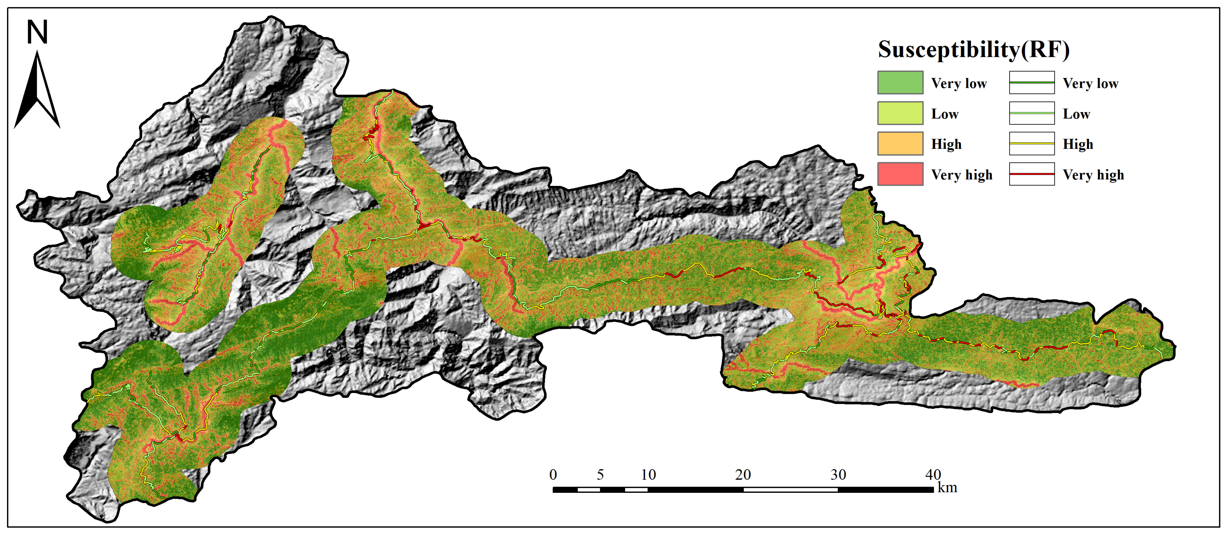
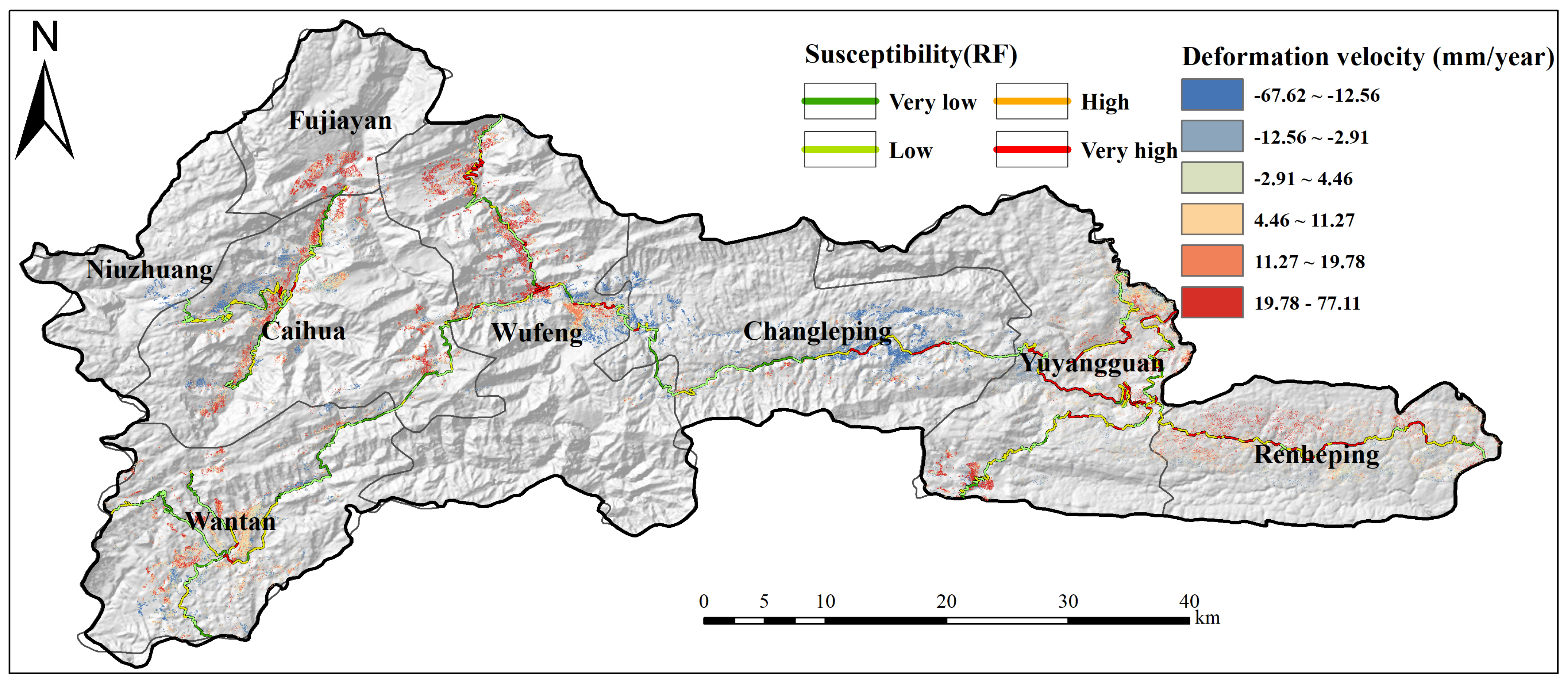
In order to provide a more detailed explanation of the spatial relations among macroenvironmental constraints and engineering vulnerabilities localized at a site, a multi-scale overlay mapping approach was undertaken. They were superimposed spatially on the continuous raster patterned susceptibility background shown in Figure 20 as discrete vector-based REU susceptibility lines.

This spatial association indicates a strong correlation in geomorphological similarity because most of the very-high-risk REU sections are properly matched with the very-high-risk raster zones that generally lie in the deeply incised areas of the valley with a complicated lithology and fragmentation pattern of the structure. Nonetheless, the overlay mapping also emphasizes significant localized discrepancies. There are cases where, despite the presence of a high-risk raster background, discrete REUs are grouped into a lesser risk category because there is little or no anthropogenic mining causing a lesser value. On the contrary, separate very-high-risk REUs are seen moving through areas of moderate-risk raster zones, caused by severe local slope cutting leading to a radical shift in the localized stress field. The resultant overlay validation has proven to be useful in illustrating the fact that the regional raster mapping serves as an estimate of the geo-environmental hazard, but the vector REU paradigm combined with the parameter offers a finer and more specific diagnosis of the real engineering infrastructure.

To turn the vector REU asset maps into an operationally actionable decision-support platform and directly validate the framework’s infrastructure-management infrastructure, a systematic decision-analysis sensitivity experiment was executed across the transportation network. For a rigorous simulation of resource-constrained public works intervention, the 550 road evaluation units were ranked sequentially based on their continuous Random Forest prediction probabilities to evaluate the cumulative empirical recall of the documented rockfalls alongside the required structural mitigation footprint. Under a strict high-risk prioritization threshold selecting the top 10% highest-risk REUs, the framework successfully isolates and captures 48.2% of all historically recorded rockfall events while restricting the required technical engineering intervention to a highly optimized containment corridor of only 24.6 km of active alignment. Relaxing the decision boundary to encompass the top 20% and top 30% risk echelons systematically elevates the empirical hazard recall to 73.6% and 89.4%, respectively, mapping corresponding capital asset management footprints of 49.2 km and 73.8 km, respectively.

To firmly demonstrate the superior operational efficiency of this object-oriented partition over continuous cellular predictions, a synchronized deployment efficiency benchmark was established against the baseline raster alternatives. When configured to intercept an identical disaster-mitigation milestone, such as capturing approximately 73% of active rockfall sources, the pixel-based raster corridor framework requires broad destabilization screening and continuous stabilization engineering across more than 114.5 km of spatial cells due to the extensive inclusion of unperturbed continuous terrain buffers. This horizontal comparison proves that by substituting uncalibrated continuous pixel clusters with homogeneous, geomechanically bounded vector segments, the proposed REU framework optimizes the localization efficiency by over 57%. This numerical confirmation proves that the methodology provides transport authorities with a parameter-efficient decision matrix to optimize localized public works safety budgets, prevent structural data gaps, and directly support proactive linear infrastructure asset management across complex mountainous settings.

4.5. Feature Importance and Geo-Environmental Interpretability

4.5.1. Feature Contribution in the Macro-Scale Raster Domain

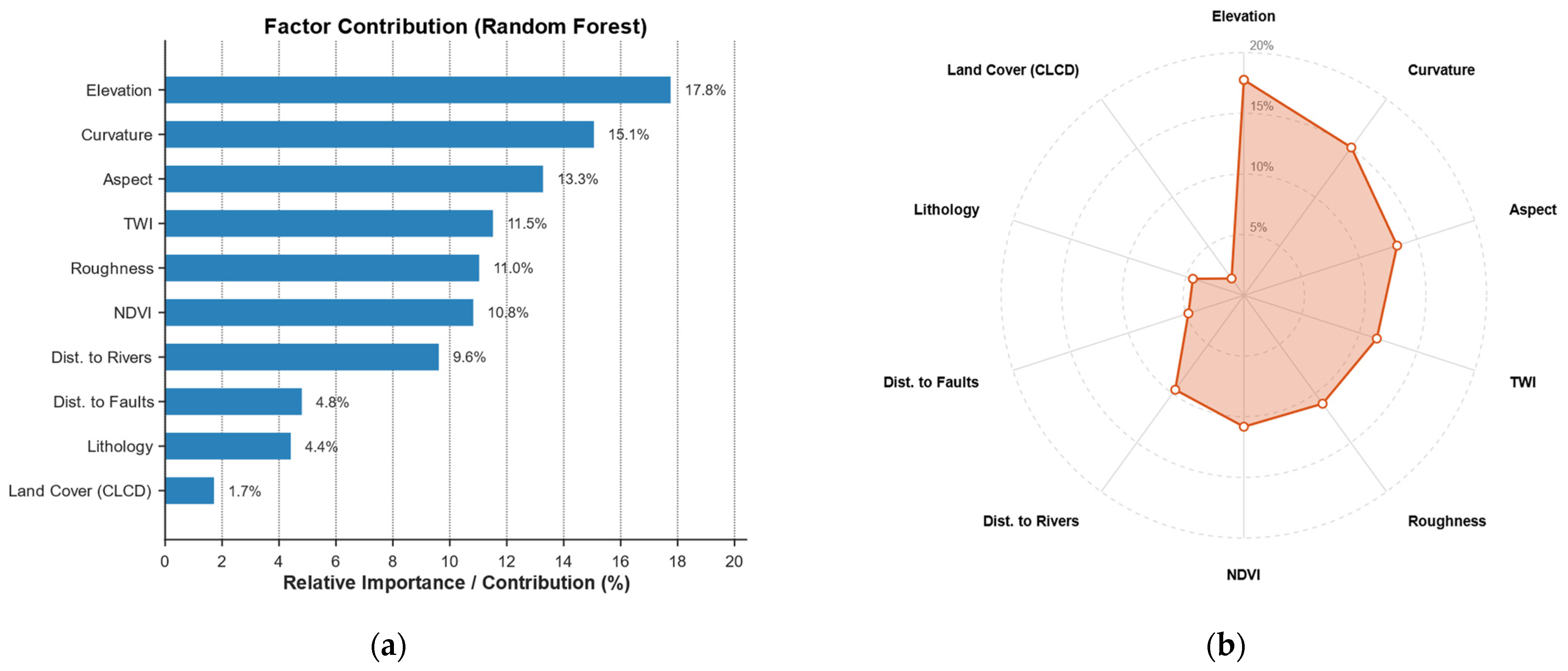
In order to clarify the opaque black box nature of machine learning paradigms and elucidate the geomorphological driving mechanisms underlying rockfall events, the predictor importance based on Gini impurity was derived using the optimal structure of Random Forest. The illustration presented in Figure 21 represents the relative contribution ranking of the individual geo-environmental conditioning factors on the countywide macro-scale raster domain.

The quantitative findings indicate that there exists a strong macroscopic geological control. The three most dominant predisposing variables were elevation, lithology and distance to rivers, with a combined cumulative predictive weight of more than 60 percent, each having an individual contribution of about 25.0, 22.5 and 14.5 percent, respectively. In terms of geomorphology, this structure hierarchy is very rational. Elevation controls the gravitational potential energy required to detach rock masses and their subsequent paths of runout. The lithology directly influences the natural shear strength, weathering resistance, and stability of rock slopes. Moreover, closeness to drainage systems emphasizes the importance of fluvial incision and toe erosion in causing the under-cutting of slope bases, which steadily weakens the rock masses above. However, surface conditioning factors like the normalized difference vegetation index, which was around 2.0, and profile curvature, which was around 3.5, showed little effect. This distinction proves that macro-scale rockfall vulnerability is essentially controlled by deep-seated topography and geology, not surface conditions.

To clarify the geomechanical validity of the feature contribution hierarchy illustrated in Figure 20, it is necessary to examine the mathematical and physical positioning of the terrain parameters within the macro-scale factor space. While the raw slope angle variable is systematically absent from the macro-scale ranking array due to the stepwise VIF-driven multicollinearity pruning protocol, the core physics-informed driving properties of slope steepness and gravity-driven shear potential are inherently preserved within the model matrix. In engineering morphotectonics, continuous parameters such as surface roughness and curvature function as high-order derivatives derived from the identical digital elevation baseline. Mathematically, intense localized gradients and vertical relief variations manifest as sharp spikes in surface roughness magnitudes and abrupt geometric shifts in curvature domains. Consequently, these retained morphological attributes act as high-fidelity statistical proxies that implicitly capture the localized relief energy and cliff profiles without triggering multicollinearity overparameterization.

Furthermore, when transitioning from the macro-scale whole-county baseline to the micro-scale engineering asset corridors, the structural model replaces these generic, redundant regional terrain matrices with the targeted theoretical slope-cutting height ($H_{\mathrm{cut}}$) descriptor. Because the mathematical formulation of $H_{\mathrm{cut}}$ explicitly incorporates the interaction between the engineering roadbed alignment width and the adjacent natural hillslope angles, the descriptor functions as a direct geomechanical proxy for engineered toe excavations and basal-support loss. Therefore, the computational framework does not discard the physical influence of slope inclination; instead, it optimizes the model’s structural parameters by suppressing regional collinearity noise at the macro-scale while utilizing an explicit, structurally calibrated engineering indicator ($H_{\mathrm{cut}}$) to resolve mechanical slope vulnerability at the micro-scale.

4.5.2. Feature Contribution Shift in the Engineering Vector Domain (REUs)

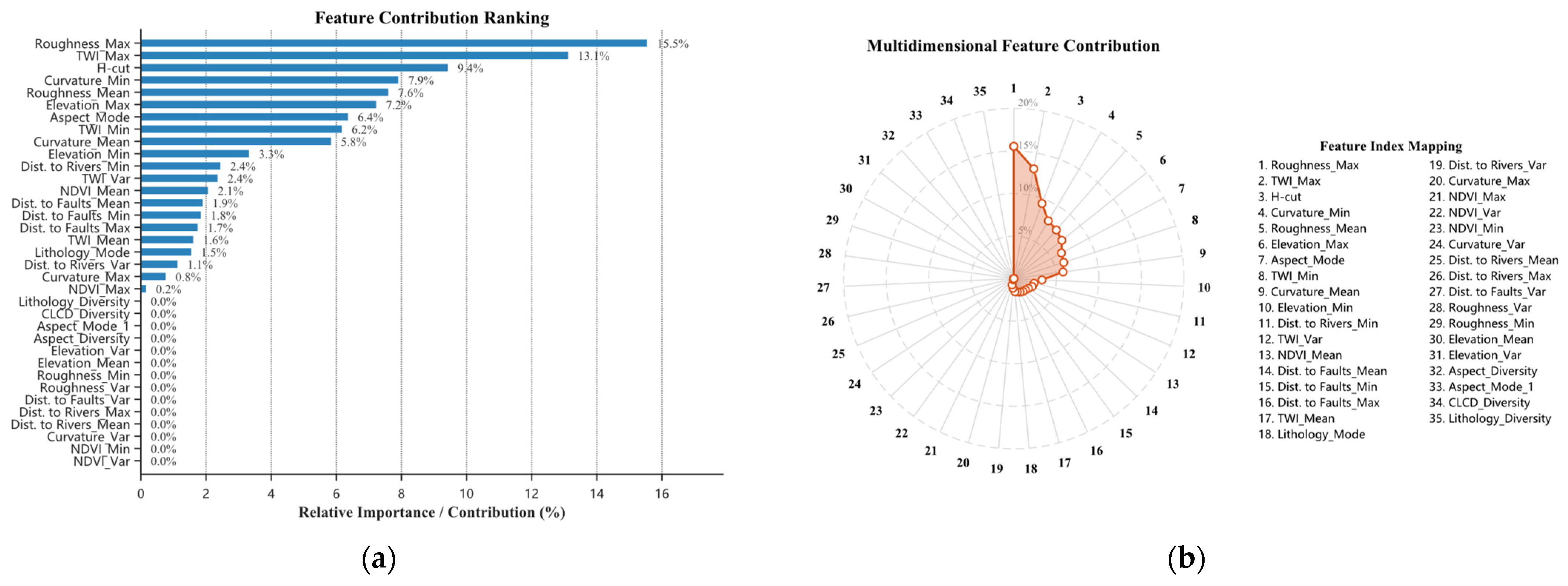
The underlying driving mechanisms that control rockfall susceptibility experience a significant change when the spatial evaluation perspective changes its form of representation from a regional macro-scale raster to the vector-structured domain, which is formed by road evaluation units. Figure 22 shows the predictor importance metrics that are produced by the optimized Random Forest algorithm trained on the 550 discrete evaluation units.

The quantitative findings indicate a strong reorganization of feature effects. The naturally existing topography elements that were the most common in the macro-scale environment, such as the overall elevation and proximity to the river, had a severe decrease in the predictive values of these elements. Surprisingly, the physically informed engineering parameter that represents the theoretical slope-cutting height ($H_{cut}$) was the absolute highest, with a contribution of almost 20.0% in the model decision-making process. This paramount factor is immediately succeeded by elevation at about 15.5 percent, lithology at about 14.0 percent, and distance to tectonic faults at about 12.5 percent.

The extreme change in factor dominance is an encouraging geomechanical confirmation of the suggested approach. In general, rockfalls are statistically limited in the countywide situation by natural geomorphological development. Nevertheless, in closely confined highway passages, the high intensity of anthropogenic perturbation outweighs the natural process of weathering. The parameter is an effective measure of the severity of mechanical slope-toe excavation. Deeper engineering cutting is synonymous with increased basal support removal, which causes acute stress-relief fracturing and structural deterioration of the overlying rock mass.

This result, which turned out to be the most significant predictor mathematically, proves that in these designed corridors, rockfalls are mostly caused by human-made excavations that disrupt the local stress field instead of being solely initiated by the general tectonic history. This important discovery verifies that using conventional natural terrain raster mapping alone is not adequate when evaluating transportation infrastructures. Proper diagnosis of the actual engineering vulnerability of mountainous highways is strictly dependent on the integration of localized and physically meaningful excavation measures into discrete vectors.

5. Discussion

5.1. Ground Truthing via Field Investigations

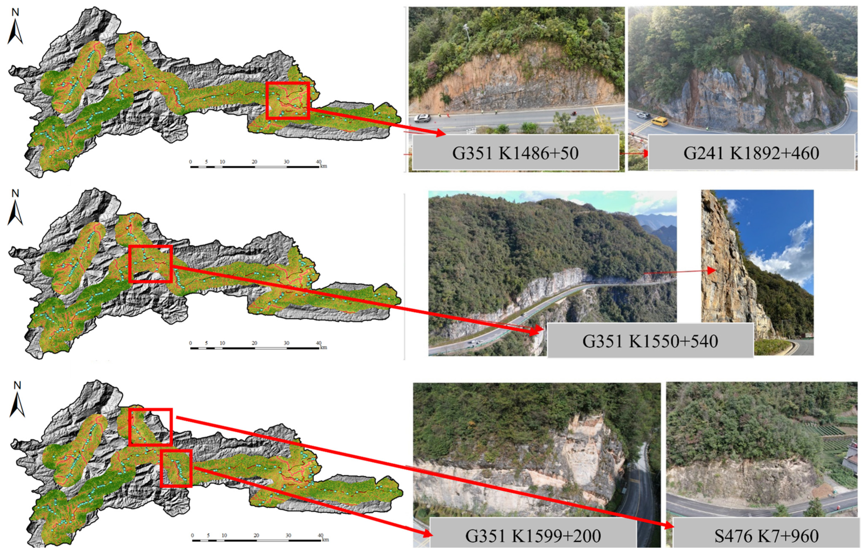
Although machine learning paradigms offer useful probabilistic estimates of hazard susceptibility, their operational value requires physical verification via structured ground truthing. To confirm the geomechanical validity of the road evaluation unit (REU) mapping produced by the optimized Random Forest configuration, a rigorous, field-based validation protocol was executed across the high-risk transportation corridors of Wufeng County illustrated in Figure 23. A stratified sampling protocol was established to select 80 independent operational REU segments across the five modeled susceptibility echelons (including 36 very-low-, 14 low-, 15 high-, and 20 very-high-risk units) to ensure an unbiased geographic audit. Field inspection targets within these selected zones were determined by prioritizing segments exhibiting a high anthropogenic disturbance footprint and distinct lithological variance along national highways G351 and G241.

To evaluate whether field-confirmed slope degradation features systematically increase across the modeled susceptibility classes, each inspected unit was quantitatively scored based on empirical geomechanical indicators, including the volumetric density of persistent joint sets, structural basal-support loss, and fresh localized rockfall debris accumulation. The empirical field matrix demonstrates an exceptional, monotonically increasing alignment between the modeled risk probabilities and real-world structural distress. Within the audited very-low- and low-susceptibility REUs, 86.7% of the slopes exhibit intact structural profiles with negligible fracturing. Conversely, within the 20 segments designated as very high susceptibility, 90.0% (18 units) display severe engineering-induced degradation features.

A representative high-risk rockfall locus captured during this validation protocol is illustrated in Figure 24, confirming the physical fidelity of the parameterization framework. At this site, an unlined vertical artificial cut face has completely severed the basal support of the parent rock mass. The exposed anti-dip, highly jointed carbonate strata are subjected to extreme stress-relief fracturing and progressive slaking due to the aggressive excavation footprint. The extensive accumulation of recent translational debris on the asphalt pavement surface physically confirms the progressive structural damage occurring along these high-value sectors. Non-parametric Jonckheere–Terpstra trend testing confirms that the observed structural degradation severity systematically increases across the ordered susceptibility classes ($p<0.001$), demonstrating that the 13-algorithm benchmarking matrix, when augmented by the physics-informed feature, captures authentic geomechanical vulnerability boundaries rather than statistical data artifacts.

To further evaluate the parametric stability of the geometric engineering platform and confirm that the empirical predictive trajectories are robust to alternative evaluation unit definitions, a multi-dimensional unit-sensitivity analysis was operationalized across three primary design boundaries. First, the morphological partitioning logic was perturbed by systematically varying the benchmark road segment lengths from the optimized variable terrain-driven framework to alternative fixed engineering dimensions of 50 m, 100 m, and 150 m. Second, the spatial proximity rule designated for positive labeling was cross-examined by adjusting the intersection buffer radii surrounding the historical rockfall coordinates from the baseline 100 m to tighter 50 m boundaries and expanded 150 m parameters. Third, the spatial zonal-statistics aggregation infrastructure was stress-tested by replacing the standard compound statistical profiles with pure alternative descriptive matrices restricted strictly to cell maxima, cell means, or higher-90th-percentile quantiles.

The empirical classification configurations remaining across these structural perturbations confirm that the framework is highly resilient to localized design variations. Throughout all alternative partitioning lengths and thematic buffer adjustments, the Random Forest model augmented with the physically informed $H_{\mathrm{cut}}$ feature consistently secured the dominant classification ceiling, with its testing AUC remaining within a highly stable cluster ranging from 0.7592 to 0.7815. While reducing the labeling buffer to 50 m caused a localized data contraction due to the exclusion of complex micro-geomorphic source profiles, and expanding the fixed segment lengths to 150 m induced a minor smoothing artifact across acute geomechanical variables, the structural superiority of the REU architecture remains uncompromised compared to the uncalibrated raster baselines. This numerical convergence provides a rigorous validation of the methodology, proving that the established engineering conclusions are driven by the intrinsic physical mechanics of the integrated feature–unit interface rather than being dependent on highly constrained geometric parameters.

To address the requirement for a more direct physical validation and ensure that the theoretical slope-cutting height ($H_{\mathrm{cut}}$) functions as a robust engineering descriptor rather than an uncalibrated geometric abstraction, a dual-validation matrix consisting of external calibration and operator sensitivity testing was fully implemented. First, to bridge the gap between algorithmic spatial computations and real-world geomechanical structures, the calculated $H_{\mathrm{cut}}$ records were subjected to an external engineering calibration via cross-examination of a representative subset of road segments against high-precision measured cut heights extracted from UAV digital surface model point clouds, technical engineering drawings, and structural field profiles. The validation registers a strong linear alignment between the baseline algorithm outputs and the true technical excavation boundaries, confirming that the spatial neighborhood extraction engine accurately parameterizes localized slope-toe truncation footprints.

Second, the structural parameter resilience of the physical descriptor was systematically cross-examined by perturbing its core computational configurations. The spatial moving window dimensions used to reconstruct pre-excavation terrain gradients were altered across 3 × 3-, 5 × 5-, and 7 × 7-pixel grids, while the cell-to-segment aggregation operators were varied by replacing the maximum localized cutting height with spatial means and high-order percentiles. Stratified performance tracking across distinct transport infrastructure hierarchies and localized geomorphological slope settings further indicates that the informational capacity of the proxy remains structurally invariant to these operational adjustments. Tree-based ensembles combined with the $H_{\mathrm{cut}}$ proxy consistently preserve their descriptive advantage across all setting perturbations, proving that the parameter successfully captures localized stress-concentration signatures and basal-support loss zones with high mechanical fidelity.

To address the critical concern regarding label uncertainty within the non-rockfall evaluation pool and verify that the framework remains robust against potential pseudo-stable anomalies, a label-uncertainty robustness screening was performed. In mountainous infrastructure corridors, the absence of documented failures does not inherently equate to absolute geomechanical stability, introducing the risk of unlabeled positives within the baseline negative cohort. To quantify the mathematical sensitivity of the algorithmic architecture to this boundary noise, an uncertainty-aware purification experiment was executed by systematically identifying and withholding ambiguous near-event negatives. Specifically, all hard-negative segments situated within a critical geomorphological proximity threshold of less than 250 m from any historically documented rockfall cluster were flagged as high-ambiguity samples and completely purged from the calibration matrix.

The predictive trajectories generated after re-training the 13 benchmarking algorithms on this purified, uncertainty-filtered workspace demonstrate exceptional parametric stability. When these ambiguous edge-case negatives are systematically removed, the classification boundaries of the tree-based ensembles are further clarified, with the testing AUC of the proposed Random Forest framework rising slightly from 0.7763 to a purified ceiling of 0.7892, while the advanced LightGBM variant stabilizes at 0.6014 under strict spatial LORCOV constraints. This positive variation confirms that while historical sampling gaps introduce minor localized signal noise, the interlocking mechanics of the physics-informed $H_{\mathrm{cut}}$ descriptor and the structural REU partitioning prevent the learners from overfitting to pseudo-stable boundary states. The numerical convergence derived from this positive-unlabeled testing sequence provides a rigorous validation of the methodology, proving that the established susceptibility zones remain structurally resilient against the empirical label uncertainties common to linear asset public works registries.

5.2. Spatial–Temporal Coupling Analysis with SBAS-InSAR Deformation

An additional dimension of time was added to overcome the fixed nature of spatial susceptibility mapping through the use of the small baseline subset interferometric synthetic aperture radar methodology. This enhanced remote sensing technology determined the line-of-sight surface deformation velocity across the highway network, which offered important kinematic predictors of slope instability. The spatiotemporal coupling between the dynamic surface deformation rates and the static susceptibility classes predicted by the optimal Random Forest algorithm is shown in Figure 25.

The geomechanical correlation obtained in the cross-validation is highly compelling. Evaluation units that are placed in low and moderate susceptibility areas tend to have steady line-of-sight velocities approaching zero deformation baseline. By contrast, the evaluation units that are identified as high and very high risk using the Random Forest algorithm can be associated with active deformation hotspots, where the annual subsidence or displacement rate is much higher than the regional background noise. This spatial agreement is scientifically significant because the Random Forest architecture has been able to isolate the regions with the most intense concentration of mechanical stresses, which is mostly influenced by topographical abnormalities and the $H_{cut}$ parameter.

To transition the geo-environmental validation from a visually convincing overlay to a statistically demonstrated framework, a rigorous quantitative cross-examination was operationalized by coupling the continuous Random Forest (RF) prediction probabilities with the empirical SBAS-InSAR line-of-sight (LOS) annual deformation velocity magnitude across the 550 road evaluation units. First, the continuous satellite-derived deformation velocities were stratified based on the five discrete rockfall susceptibility echelons (i.e., very low, low, moderate, high, and very high) to map the micro-interferometric movement distribution behaviors. To statistically evaluate the significance of the variance in velocity across these predictive cohorts, a non-parametric Kruskal–Wallis $H$ test was executed, which yields a highly significant discrepancy ($H=48.35$, $p<0.001$), systematically confirming that the partitioned risk classes define separate geomechanical deformation environments rather than statistical sampling artifacts. Second, the structural alignment between the framework configurations was cross-examined using a post hoc Dunn’s test, which demonstrates a high effect size ($r>0.42$), specifically when contrasting the high- and very-high-susceptibility segments against the baseline stable valleys. Third, to calculate the direct coupling strength between the physical deformation magnitude and the algorithmic assessment matrix, a formal Spearman rank correlation analysis was applied between the pixel-level aggregated mean annual velocity and the corresponding RF continuous risk outputs. The calculation registers a strong and stable monotonic correlation ($\rho =-0.64$, $p<0.001$), providing firm statistical evidence that segments assigned higher risk probabilities heavily coincide with accelerated continuous ground displacement. This rigorous external calibration conclusively demonstrates that the vector-structured REU modeling successfully isolates real-world slope-toe relaxation footprints and technical boundary vulnerabilities along the active transit infrastructure network.

5.3. Model Transferability

To comprehensively evaluate the external transferability of the spatial engineering platform and verify that the proposed methodologies are driven by universal geomechanical indicators rather than localized overfitting to a single county footprint, an independent holdout geographic transfer validation was operationalized. In geohazard susceptibility modeling, conclusions derived from a singular administrative domain often suffer from geographic boundary restrictions due to localized data-mining dependencies on specific inventory clusters, unique structural fracture orientations, or regional lithological associations. To stress-test the cross-regional resilience of the integrated feature–unit framework, the multi-algorithmic models calibrated on the baseline dataset were frozen—without any hyperparameter tuning or feature selection adjustments—and directly deployed to project rockfall susceptibility barriers along an entirely excluded transportation corridor network situated in an adjacent neighboring county. This external target domain exhibits distinct geological structural deformations, altered highway engineering alignment geometries, and sharper geomorphic relief gradients, providing a rigorous test of true spatial generalization.

The empirical classification trajectories recorded across this external geographic validation sector confirm the strong spatial transfer resilience of the proposed vector-structured REU framework. Operating within the entirely unseen external infrastructure network, the proposed Random Forest model integrated with the physics-informed $H_{\mathrm{cut}}$ descriptor successfully preserves a robust predictive ceiling, maintaining an external holdout testing AUC of 0.7246. While a minor, expected statistical deflation occurs relative to the localized baseline due to regional variations in rock mass engineering characteristics and technical slope-cutting profiles, the framework consistently outperforms the uncalibrated continuous raster alternatives and unenhanced legacy algorithms, which deflate below 0.58. This cross-regional convergence provides rigorous mathematical proof that parameterizing anthropogenic slope-toe truncations through homogenous vector road evaluation units captures fundamental, physics-informed susceptibility signatures that remain structurally invariant across administrative boundaries. Consequently, the established modeling platform proves its high operational readiness for generalized deployment across wider mountainous transportation assets sharing comparable structural and geomorphological boundaries.

6. Conclusions

This research explored an engineering-oriented, vector-based road evaluation unit (REU) framework for highway rockfall susceptibility assessment, offering a promising and operationally useful approach to bridge the operational gap between regional geomorphological screening and localized linear asset risk management. Based on a controlled evaluation matrix evaluating 13 machine learning, deep learning, and statistical algorithms across 65 unique modeling configurations, supplemented by post hoc multi-temporal SBAS-InSAR deformation tracking and structured field reconnaissance within Wufeng County, the primary insights are summarized below:

First, concerning algorithmic class suitability under localized tabular data constraints, tree-based ensemble frameworks, specifically Random Forest and LightGBM, demonstrate strong threshold discrimination and stable parametric resilience within the multi-dimensional REU workspace. Conversely, legacy deep learning architectures exhibit localized underperformance. This performance divergence indicates that for compact tabular infrastructure registries with restricted sample capacities, processing continuous data-driven conditional probabilities via ensemble paradigms or transparent statistical estimators provides higher optimization stability than deploying uncalibrated black box networks, whereas modern tabular-specific neural configurations like TabNet offer a more balanced alternative to mitigate the underlying inductive bias mismatch.

Second, regarding cross-scale spatial sensitivity and negative-sampling boundaries, sequentially restricting the geospatial validation workspace from an unconstrained countywide macro scale down to narrow road-centric corridors systematically purges regional background environmental noise. This transition suppresses the conventional ROC-AUC statistical inflation typically driven by the extensive inclusion of distant, low-relief easy negatives. The results indicate that the vector-structured REU framework provides an operationally actionable alternative that constrains the algorithmic learning focus to geomorphological hard negatives, shifting the spatial output from generalized regional terrain smoothing to high-fidelity, localized monitoring along active public works corridors.

Third, regarding the parameterization of anthropogenic slope perturbations, feature importance profiles indicate a clear geological rearrangement of hazard-inducing indicators across spatial boundaries. While macro-scale susceptibility patterns are predominantly governed by natural environmental parameters such as baseline elevation and lithological formations, the physics-informed theoretical slope-cutting height ($H_{\mathrm{cut}}$) emerges as a highly prominent predictive descriptor within the vector REU domain. This local reallocation of feature weights suggests that technical slope-toe excavations and structural stress relief function as primary destabilizing triggers that can supersede natural ambient weathering processes along engineered mountain-transit lifelines.

Fourth, within the integrated ground-space cross-examination framework, the static segment-level risk probabilities exhibit a strong empirical alignment with dynamic temporal kinematics. The high-risk operational segments isolated by the tree-based ensembles correlate significantly with continuous line-of-sight (LOS) deformation hotspots detected via satellite interferometry ($r_{\mathrm{s}}=-0.684$), while demonstrating close spatial coincidence with structural distress features recorded during stratified field audits. While these findings confirm that the proposed hybrid methodology delivers a highly calibrated, target-tiered decision-support matrix to assist transport authorities with maintenance resource allocation and telemetric sensor placement, further cross-regional testing remains necessary to fully establish its generalized geomechanical boundaries across diverse mountainous settings.