Article

Analysis and Intelligent Processing of the Underwater Navigation Adaptability of Gravity Reference Maps


State Key Laboratory of Spatial Datum, Xi’an 710054, China
*
Author to whom correspondence should be addressed.
Remote Sens. 2026, 18(16), 2812; https://doi.org/10.3390/rs18162812
Submission received: 14 March 2026 / Revised: 30 April 2026 / Accepted: 11 May 2026 / Published: 19 August 2026

Highlights

What are the main findings?
  • Nine characteristic parameters of gravity anomaly, including standard deviation and roughness, were constructed. The comprehensive evaluation of the gravity reference map suitability was realized using the sliding window method and factor analysis, which effectively solves the problem of insufficient accuracy in single-parameter evaluation.
  • Simulation verification using the TERCOM algorithm reveals limitations of traditional statistical methods. On this basis, two intelligent algorithms, the learning vector quantization neural network and extreme learning machine, were proposed and verified, among which the extreme learning machine performs better in classification efficiency and accuracy.
What are the implications of the main findings?
  • This study improves the indicator system and statistical evaluation framework for gravity reference map suitability assessment, which can provide a theoretical basis for regional optimization and path planning in underwater gravity-matching navigation.
  • The introduction of intelligent algorithms compensates for the shortcomings of traditional statistical methods, enhances the reliability and practicability of gravity suitability classification and prediction, and has practical application value for improving the long-endurance navigation accuracy and safety of underwater vehicles.

Abstract

Gravity-matching navigation is one of the important means for the covert navigation of underwater vehicles. The production and application of gravity reference maps as core key technologies have a very significant impact on the accuracy of underwater navigation. Firstly, this paper adopts the factor analysis method to obtain the comprehensive results of nine characteristic parameters such as the standard deviation and roughness of the gravity reference map by setting a range sliding window. Secondly, the TERCOM algorithm is introduced to conduct simulation verification calculations within the sliding window. After comparing and verifying with the comprehensive results of the factor analysis characteristic parameters, the limitations of statistical methods in the evaluation of the adaptability of gravity reference maps are analyzed. Thirdly, intelligent processing methods such as the learning vector quantization neural network algorithm and the extreme learning machine are proposed. The characteristic parameters of some sliding window gravity reference maps and the simulation verification results of the TERCOM algorithm are used as training samples to predict the adaptability evaluation effect of underwater gravity navigation for other sliding windows. The results show that the prediction results are generally in good agreement with the simulation verification results of the TERCOM algorithm. Compared with the learning vector quantization neural network algorithm, the extreme learning machine algorithm exhibits superior performance in terms of classification accuracy and computational efficiency.

1. Introduction

The characteristics of gravity reference maps in different sea areas vary, and their adaptability also differs [1,2]. Conducting adaptability evaluations in advance can provide reasonable references for navigation path planning, improve matching accuracy, and effectively avoid adverse interferences such as ocean currents and hidden reefs.
To evaluate the gravity-matching navigation effects in different regions, Reference [3] proposed a criterion for selecting matching areas based on the gravity gradient tensor. Reference [4] suggested using principal component analysis and an analytic hierarchy process for selecting matching areas in gravity gradient matching. Reference [5] proposed an adaptability analysis method based on multi-attribute decision-making theory. Reference [6] converted local gravity maps into 8-bit grayscale images and proposed a gravitational field algorithm to evaluate the navigable characteristics of the gravity maps. Reference [1], based on fractal geometry theory, analyzed the spectral characteristics of three-dimensional surface gravity anomaly sequences and proposed an isotropy coefficient as a feature parameter to represent the directionality of the gravity-matching area; they combined traditional gravity parameters with the isotropy coefficient using the analytic hierarchy process to establish a comprehensive feature parameter. Reference [7] constructed new gravity anomaly feature parameters; they calculated the gravity-matching-assisted navigation feature values of 13 regions in the Western Pacific and conducted navigation simulation experiments. Reference [8] introduced the average gravity difference (AGD) parameter to represent the gravity variation level of a certain area. Through a comprehensive investigation of global ocean gravity, they calculated and analyzed the AGD values of local areas. After a series of experiments, they roughly determined the relationship between the AGD values of local areas and navigation accuracy and derived the selection criteria for matching areas. Reference [9] proposed gravity anomaly and vector difference parameters to obtain the matching applicability in direction. They used the entropy method to integrate the proposed vector difference parameters with traditional gravity feature parameters to obtain comprehensive feature parameters. Reference [10] started from vector features and spatial relationship features and proposed a matching area selection algorithm based on Delaunay triangulation; they used a comprehensive feature matrix and conducted feature extraction and cluster analysis to select matching areas. Reference [11] proposed a matching area selection algorithm based on co-occurrence matrices for the spatial relationship features of the gravity field. They established a co-occurrence matrix of gravity anomalies to extract spatial relative feature parameters; they used entropy to establish comprehensive spatial feature parameters and selected matching areas through maximizing the variance between classes. Reference [12] proposed a convolution slope parameter-support vector machine combination method. They used the Sobel operator to convolve the gravity anomaly map to obtain a feature map; they combined the feature map and the gravity anomaly map to construct the convolution slope parameter and combined the convolution row and column differences in the feature map, the convolution variance of the feature map, and the range of the gravity anomaly map as feature parameters. Reference [13] comprehensively considered multiple terrain feature parameters and proposed a multi-index comprehensive decision-making evaluation method based on gray fuzzy theory. To address the issue that different matching routes have different navigability in specific terrains, they proposed a navigation coefficient analysis based on terrain statistical parameters to compare the navigability of different routes. Reference [14] analyzed the key factors influencing navigation error, including heading, matching length, inertial navigation initial position error, gravimeter error, map error, and inertial navigation drift. They took these experimental conditions as prior information and proposed a conditional probability-based MCA calculation method to estimate the matching probability within the required error range in a given digital gravity map. Reference [15] also proposed a frequency-domain matching area selection method based on high-resolution features of the gravity gradient, using wavelet transform to extract high-frequency information from the gravity gradient reference map and establishing a gravity gradient wavelet transform model. They also proposed a morphological image-texturing method to obtain texture density, texture amplitude, and texture direction within the matching area, achieving a matching rate higher than 90%. Reference [16] focused on optimizing the matching area selection in underwater gravity-matching navigation. They proposed a new gravity field feature parameter selection method based on feature selection principles and SVM, screening five key parameters from 14 candidates and integrating them with SVM to construct a classification model. Reference [17] aimed to improve the accuracy of selecting navigation adaptation areas for gravity-aided navigation. They constructed a gravity field feature set using a gray-level co-occurrence matrix, a local binary pattern and a proposed normalized gravity scale, and designed a deep gravity field perception model with an inter-layer propagation mechanism for model training. Reference [18] intended to improve the matching accuracy and track continuity of underwater gravity-aided navigation. They designed a curvature directional feature based on principal and Gaussian curvature, and proposed a two-stage matching area re-closing mechanism combining morphological operations and cluster-based status updates. Reference [19] aimed to quantify the directional adaptability of gravity anomaly maps for gravity-aided inertial navigation. They designed three directional parameters and constructed a balanced gravity characteristic parameter, then used an LM-BP neural network to model the mapping between these features and directional matching rates, establishing an adaptability evaluation framework.
The above methods all evaluate the adaptability of gravity navigation from a statistical or frequency-domain analysis perspective. This paper adopts a sliding window method, defines characteristic parameters such as the standard deviation and roughness of gravity anomalies, and compares the simulation verification results of factor analysis methods and TERCOM algorithms. It analyzes the limitations of statistical methods in evaluating the adaptability of gravity reference maps and proposes the use of intelligent processing methods such as vector quantization neural network algorithms and extreme learning machines for classification and prediction, and conducts verification calculations.

2. Characteristic Parameters

2.1. Parameter Definitions

The overall changes in marine gravity reference maps are relatively small, and they can maintain a stable state for a long time. They also have various forms. Parameters such as standard deviation, roughness, information entropy, correlation coefficient, and terrain slope can be used to describe their detailed variations. These characteristic parameters describe the dispersion of gravity anomaly data within the region, the similarity between different data, and the extent of change [20]. The definitions of each parameter are as follows:
(1)
Standard Deviation of Gravity Anomaly
σ = 1 m n − 1 ∑ i = 1 m ∑ j = 1 n f i , j − f ¯ 2
f ¯ = 1 m n ∑ i = 1 m ∑ j = 1 n f i , j
In the formula, m and n represent the number of grids of the gravity field in the x and y directions within the moving window; σ is the standard deviation of the gravity anomaly, mainly reflecting the degree of dispersion of the reference map and its overall undulation; f i , j is the gravity anomaly at the grid coordinate i , j ; f ¯ is the average value of the gravity anomaly; when f i , j diverges, σ is larger, and when f i , j is concentrated, σ is smaller.
(2)
Roughness
Roughness σ z reflects the local undulation degree of the gravity reference map.
σ z = R l o n g i t u d e + R l a t i t u d e / 2
R l o n g i t u d e = 1 n m − 1 ∑ i = 1 m − 1 ∑ j = 1 n f i , j − f i + 1 , j
R l a t i t u d e = 1 m n − 1 ∑ i = 1 m ∑ j = 1 n − 1 f i , j − f i , j + 1
In the formula, R l o n g i t u d e and R l a t i t u d e represent the absolute roughness of the gravity anomaly along the meridional and zonal directions, respectively. The parameter σ z is the mean smoothness of the gravity anomaly within the calculation window and can describe relatively subtle local variations.
(3)
Convolution of Standard Deviation and Absolute Roughness
The standard deviation of the gravity anomaly reflects the overall characteristics on a macroscopic scale, while the roughness reflects the magnitude of variations on a microscopic scale. Given that the gravity anomaly reference map has a resolution of 1 ′ × 1 ′ , if the gravity anomaly values between adjacent grid points change very little, even less than 1 mGal, the variations in gravimeter measurement accuracy may be obscured by measurement noise. To address this issue, Reference [7] proposed integrating the standard deviation and absolute roughness of the gravity anomaly into a single parameter Γ i j , as follows:
S l a t i t u d e = f i , j − f i , j − k 2 + f i , j − f i , j + k 2
S l o n g i t u d e = f i , j − f i − k , j 2 + f i , j − f i + k , j 2
Γ i , j = S l o n g i t u d e + S l a t i t u d e / 4
In the formula, S l a t i t u d e and S l o n g i t u d e are the sums of squares of the gravity anomaly differences between point i , j and two adjacent points at a distance k in the longitudinal and latitudinal directions, respectively. Γ i , j is the gravity anomaly characteristic parameter for a single calculation point. Figure 1 shows the schematic diagram for calculating the convolution parameter at calculation point i , j . To utilize the m × n grid within the window to reflect the characteristic values of a larger regional area, the following function is constructed:
Γ k = 1 m n − 1 ∑ i = 1 m ∑ j = 1 n Γ 2 i , j
(4)
Information Entropy
This characteristic parameter can serve as a measure of the average amount of information. The smaller the entropy, the more dramatic the changes in the gravity background field, indicating better suitability for matching navigation. It is defined as follows:
H = − ∑ i = 1 m ∑ j = 1 n − 1 p i , j · log 2 p i , j
where
p i , j = f ( i , j ) ∑ i = 1 M ∑ j = 1 N f ( i , j )
When the base of the logarithm is equal to 2, the unit of entropy is the bit.
(5)
Kurtosis Coefficient
“Kurtosis” is used to reflect the flatness or peakedness of a data distribution, indicating the degree of concentration of values within a sliding window. It is inversely proportional to the suitability and is defined as follows:
C = 1 M N ∑ i = 1 M ∑ j = 1 N f ( i , j ) − f ¯ 4 σ 4 − 3
(6)
Skewness Coefficient
“Skewness” reflects the symmetry of the gravity reference map and is directly proportional to the suitability. It is defined as follows:
G = 1 M N ∑ i = 1 M ∑ j = 1 N f ( i , j ) − f ¯ 3 σ 3
It is a measure of the symmetry of a data distribution.
(7)
Correlation Coefficient
The correlation coefficient can be used to determine whether data are independent. The smaller the correlation coefficient, the more abundant the information in the gravity reference map, and the better the matching effect. It is defined as follows:
Q = Q l o n + Q l a t 2
where Q l o n and Q l a t represent the correlation coefficients in the longitudinal and latitudinal directions, respectively.
Q l o n = ∑ i = 1 M ∑ j = 1 N f i , j − f ¯ f i , j + 1 − f ¯ M N − 1 σ 2
Q l a t = ∑ i = 1 M ∑ j = 1 N f i , j − f ¯ f i + 1 , j − f ¯ N M − 1 σ 2
(8)
Standard Deviation of Slope
The standard deviation of slope is determined by the rate of change in the gravity reference map in the northward and eastward directions at a certain point. The formula is as follows:
S i , j = S x i , j 2 + S y i , j 2
where S x i , j and S y i , j are the eastward and northward rates of change at point i , j , respectively, and are calculated as follows:
S x i , j = f i + 1 , j + 1 + f i , j + 1 + f i − 1 , j + 1 − f i + 1 , j − 1 − f i , j − 1 − f i − 1 , j − 1 6 S y i , j = f i + 1 , j + 1 + f i + 1 , j + f i + 1 , j − 1 − f i − 1 , j + 1 − f i − 1 , j − f i − 1 , j − 1 6
The slope value S i , j is specific to each grid point in the gravity reference map. In calculations, the standard deviation is typically used to describe the slope conditions of the background map across the entire matching area:
S σ = 1 M 1 − 2 M 2 − 2 − 1 ∑ i = 2 M 1 − 1 ∑ j = 2 M 2 − 1 S i , j − S ¯ 2
S ¯ = 1 M 1 − 2 M 2 − 2 ∑ i = 2 M 1 − 1 ∑ j = 2 M 2 − 1 S i , j
(9)
Mean Cumulative Gradient
The larger the cumulative gradient, the greater the amount of information contained in the reference map. The formula is
G = 1 M 1 - 2 M 2 - 2 ∑ i = 2 M 1 − 1 ∑ j = 2 M 2 − 1 G x i , j 2 + G y i , j 2
G x i , j = f i + 1 , j − f i , j G y i , j = f i , j + 1 − f i , j
where G x i , j and G y i , j are the eastward and northward gradient values at point i , j , respectively.

2.2. Calculation and Analysis

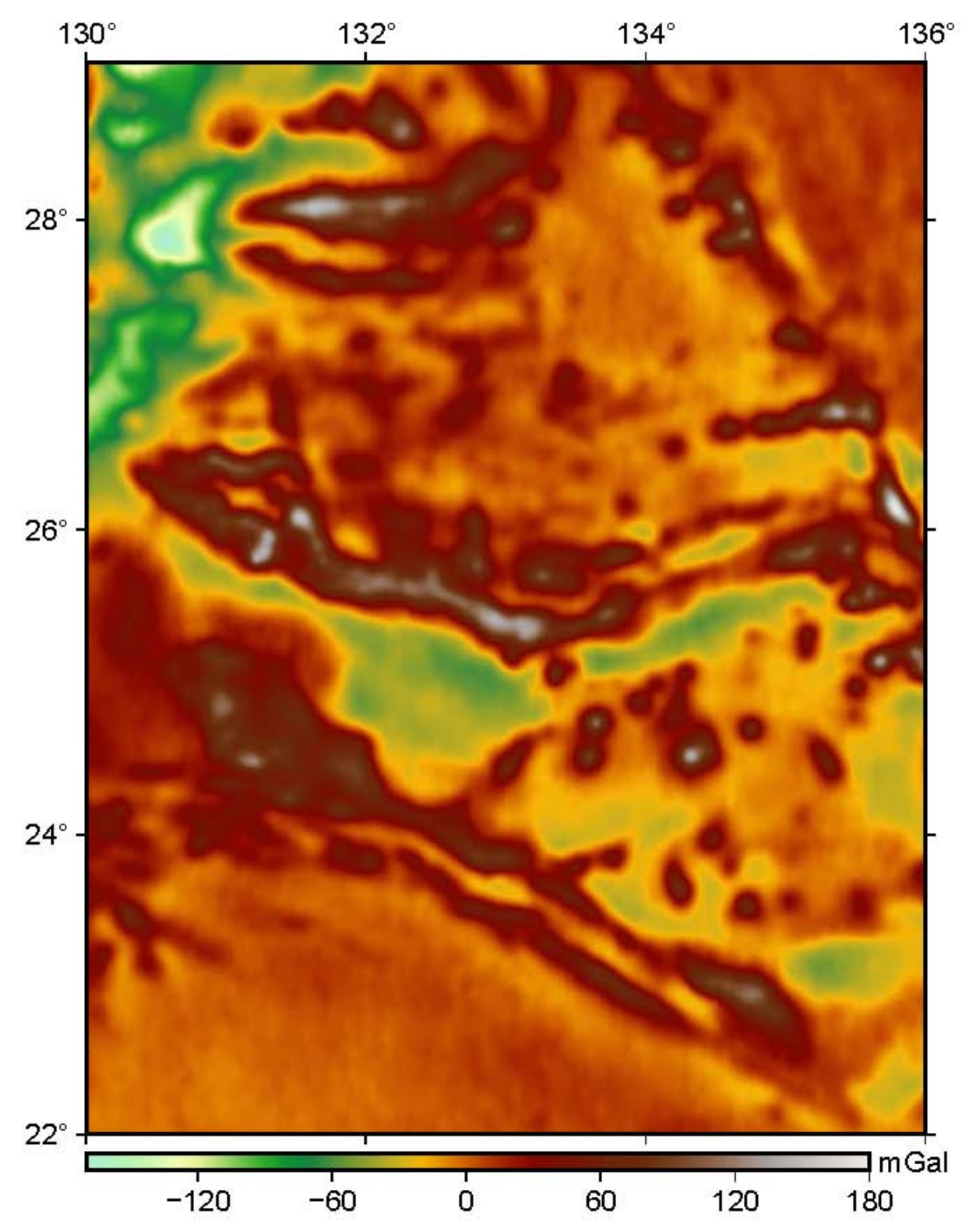
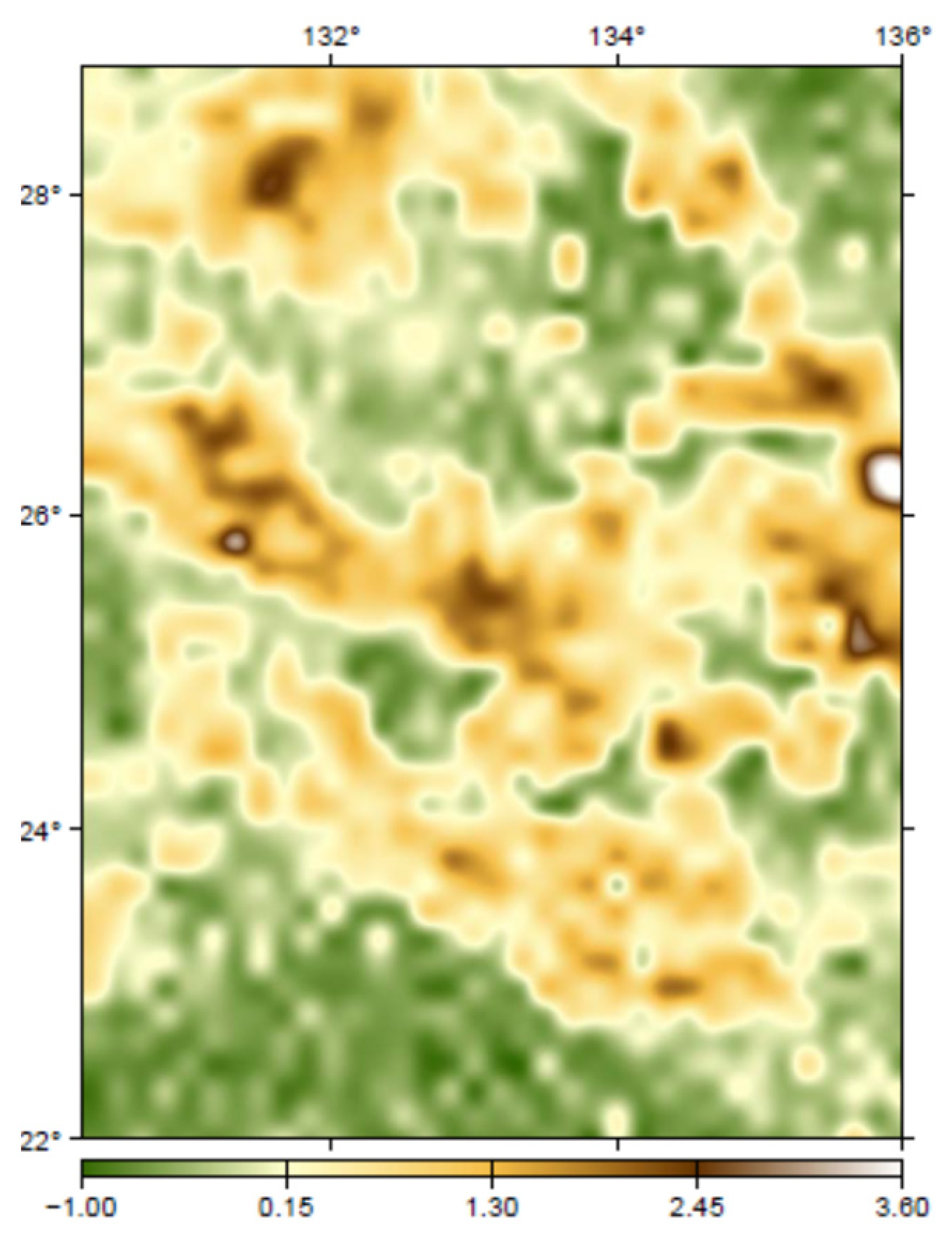
A specific area in the Pacific Ocean (22–29°N, 130–136°E) was selected as the study area. Figure 2 shows a gravity reference map constructed based on the 1 ′ × 1 ′ global ocean gravity anomaly model grav.img 24.1 released by the Scripps Institution of Oceanography. The map has an accuracy of 3 to 8 mGal, with grid points of 361 × 421, a maximum value of 180 mGal, a minimum value of −170 mGal, an average value of 7.81 mGal, and a standard deviation of 26.85 mGal. Currently, the measurement accuracy of LaCoste & Romberg and KSS31 marine gravimeters under relatively harsh sea conditions is ±1.0 mGal. Considering the influence of other types of errors (such as zero drift correction, Eötvös correction, inaccurate positioning, and spatial correction), the instrument measurement accuracy is conservatively estimated to be between ±1.0 mGal and ±2.0 mGal, which can be used for gravity-matching navigation.
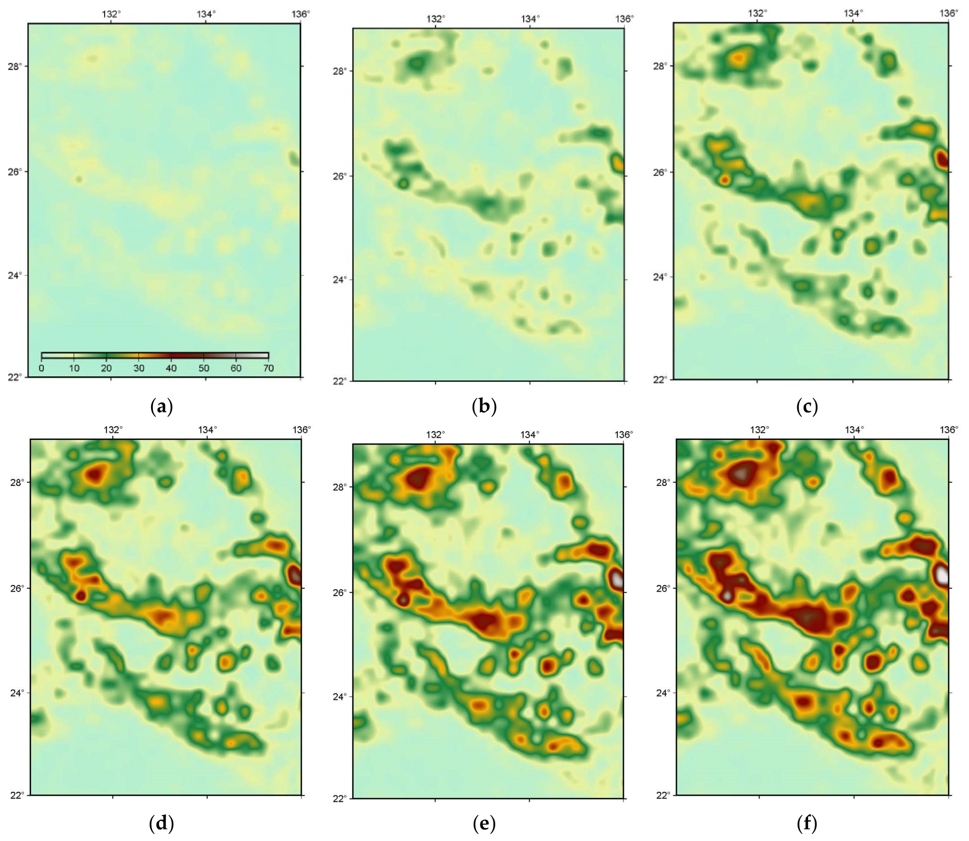
To analyze the statistical characteristic parameters of the gravity reference map in the study area, a 1 0 ′ × 1 0 ′ sliding calculation window was defined, and the calculation formulas in Section 2.1 were used to obtain various statistical characteristic parameters of the gravity reference map. In the convolution calculation of standard deviation and absolute roughness, only the integration results when the distance k between adjacent points and the moving point is between 1 and 6 were considered. When Γ k = 4 , 5 , 6 is greater than 9.3, the gravity-matching navigation in this area can achieve the optimal positioning accuracy of ± k max Γ k / 2 n m [7].
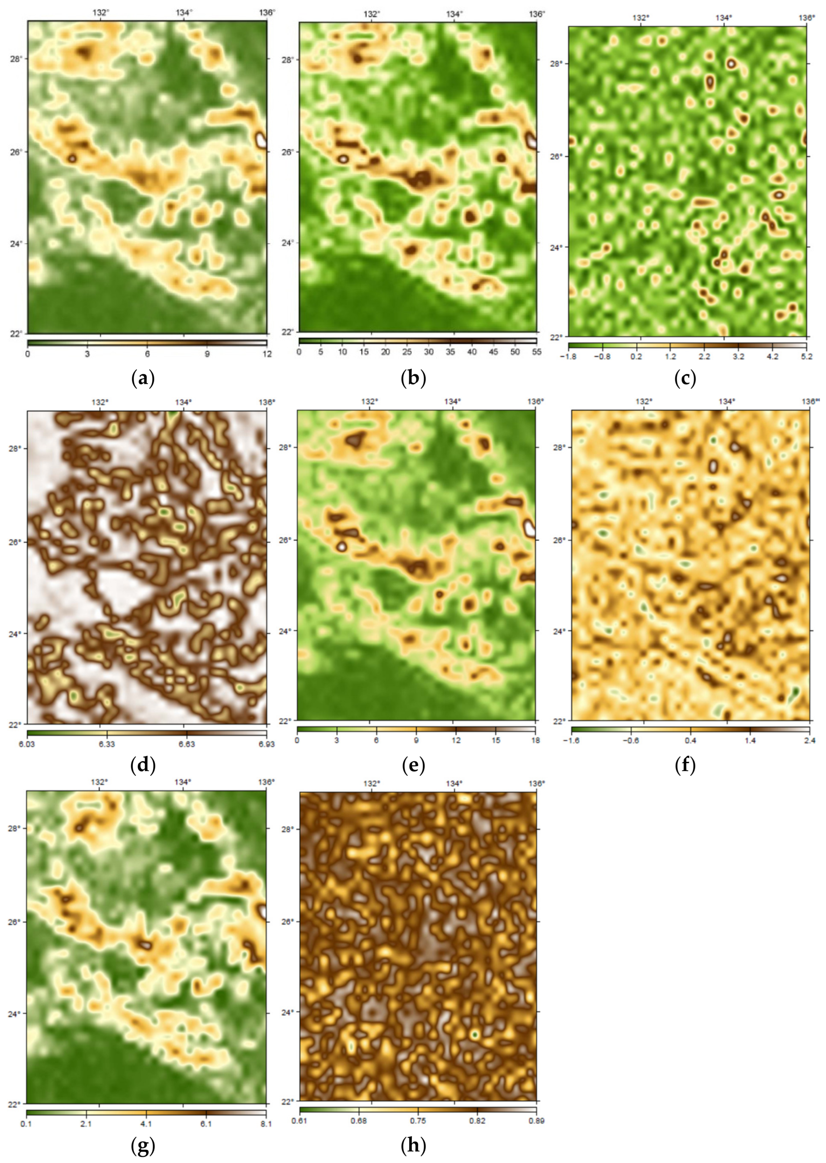
The gravity reference map serves as the foundation for underwater vehicle navigation path planning. Figure 3 shows the characteristic parameter values of the standard deviation and absolute roughness convolution when k = 1 , 2 , 3 , 4 , 5 , 6 , while Figure 4 illustrates eight other characteristic parameters. It can be observed that: ① Five parameters, including gravity anomaly convolution, roughness, standard deviation of gravity anomaly, and cumulative gradient mean, exhibit similarities. In regions with significant characteristic parameters, the gravity reference map shows drastic changes. Specifically, in the central and northwestern sea areas, the gravity values display a trend of sharp decline followed by a sudden rise. ② The suitability of different regions, as reflected by various characteristic parameters, differs. Using a single parameter may lead to multiple evaluation standards, making it necessary to comprehensively process multiple characteristic parameters. ③ For the convolution characteristic parameters of standard deviation and absolute roughness, as the k value continuously increases, the number of grid points involved in the calculation grows, and the increase in the value becomes larger. The more significant the gravity anomaly changes in a sea area, the greater its contribution to the value. In areas with gentle gravity anomaly changes, such as the southern sea area, the contribution to the value is extremely small.
The above presents nine parameters for evaluating the suitability of the background map. The single-strategy approach, which uses artificially set thresholds, involves significant subjectivity and experiential influence, potentially leading to conflicting outcomes in the determination criteria. Factor analysis, as one of the classifier strategies, can integrate different characteristic parameters and minimize subjectivity to the greatest extent.

3. Factor Analysis Method

3.1. Basic Principles

The basic idea of factor analysis is to group variables based on the magnitude of their correlations, with each group of variables representing a factor [21,22]. The specific steps are as follows: ① using a sliding window method, the gravity reference map of the study area is divided into calculation windows of the same size, and characteristic parameter values are obtained by calculating each window; ② parameters with highly consistent characteristic information are merged to obtain a simplified set; ③ information from the simplified set is extracted and summarized to obtain the main factors, which are then named and interpreted.
Assume that the number of original variables is m , and the number of indicators in each variable is n , denoted by x 1 , x 2 , x 3 , … , x n . Considering the differences in characteristic parameters, standardization must first be performed. Using k factors ( F 1 , F 2 , F 3 , … , F k ) to represent the original data, the mathematical model of factor analysis is expressed as
x 1 = a 11 F 1 + a 12 F 2 + …… + a 1 k F k + ε 1 x 2 = a 21 F 1 + a 22 F 2 + …… + a 2 k F k + ε 2 …… x n = a n 1 F 1 + a n 2 F 2 + …… + a n k F k + ε n
It is expressed in matrix form as X = A F + ε , where A , F and ε represent the loading matrix, common factors, and specific factors, respectively. The loading matrix A can also be expressed as
A = a 11 a 12 a 13 … a 1 k a 21 a 22 a 23 … a 2 k       …   a n 1 a n 2 a n 3 … a n k
The F common factors are uncorrelated, and their variances are 1; each of the ε specific factors are uncorrelated, and their variances are not required to be equal.
D F = D F = 1     0   1         …   0     1                 D ε = D ε = σ 1 2     0   σ 2 2         …   0     σ q 2
The common factors and the specific factors are also uncorrelated with each other; that is, C o v F , ε = 0 .

3.2. Program Steps

To determine whether the variables to be analyzed are suitable for factor analysis, the main methods include Bartlett’s test of sphericity, the correlation coefficient matrix test, and the Kaiser–Meyer–Olkin (KMO) test. The input raw data is standardized. For positive indicators, the formula is
y i j = a i j − min a i j max i a i j − min i a i j
For negative indicators, the formula is
y i j = min i a i j − a i j max i a i j − min i a i j
where max i a i j represents the maximum value of a specific characteristic parameter; min i a i j represents the minimum value of a specific characteristic parameter; y i j is the normalized data; a i j is the original data.
The principal components of the common factors X 1 , X 2 X 2 , …, X m are a synthesis of the original variables. The principal component method is used to solve the loading matrix:
① Calculate the standardized covariance matrix Σ ;
② Obtain the eigenvalues λ λ 1 , λ 2 , … , λ p > 0 and eigenvectors γ 1 , γ 2 , γ 3 , … , γ q of the correlation coefficient matrix;
③ Using the first m eigenvalues and their corresponding eigenvectors, calculate the solution for the loading matrix containing m factors:
B ⌢ = λ 1 γ 1 , λ 2 γ 2 , … , λ m γ m
The covariance between the standardized variables and the common factors is
C o v X F i , F j = C o v ∑ k = 1 m a i k F k + ε i , F j = C o v ∑ k = 1 m a i k F k , F j + C o v ε i , F j = a i j       i = 1 , 2 , … , n ; j = 1 , 2 , … , m
To make the original factor variables more interpretable, factor rotation is required. The main methods include orthogonal rotation and oblique rotation. Once the factor loading matrix is determined, the factor scores are calculated. The matrix expression for the estimated factor values after rotation is
F ⌢ = A * T Σ − 1 X F = W X F
where W is the factor score coefficient matrix of m × k .
(1)
Correlation Matrix
If most of the coefficients in the correlation matrix are less than 0.3, factor analysis is not suitable. Table 1 shows the correlation matrix of the characteristic parameters. Due to the similarity between the standard deviation and the absolute roughness convolution for different radii k , these parameters are merged, and the case of k = 4 is used for the correlation matrix calculation. It can be observed that the correlations among some factors, such as Γ 4 , standard deviation, roughness, slope standard deviation, and cumulative gradient mean, are mostly above 0.9; the correlation coefficients for the correlation coefficient and kurtosis coefficient are above 0.6; while the information entropy and skewness coefficient have relatively low correlations with other variables.
(2)
KMO and Bartlett’s Test of Sphericity
The KMO statistic ranges between 0 and 1. Generally, it is considered that a KMO value above 0.9 is very good, 0.8–0.9 is good, 0.7–0.8 is average, 0.6–0.7 is poor, and 0.5–0.6 is very poor. The KMO value in Table 2 is 0.827, indicating that factor analysis is appropriate. Bartlett’s test of sphericity compares the observed correlation matrix with the identity matrix to check whether there is some redundancy among the variables. A smaller significance level (<0.05) indicates that meaningful relationships exist among the original variables. The significance value in Table 2 is 0, indicating that factor analysis is suitable.
(3)
Determining the Number of Factors
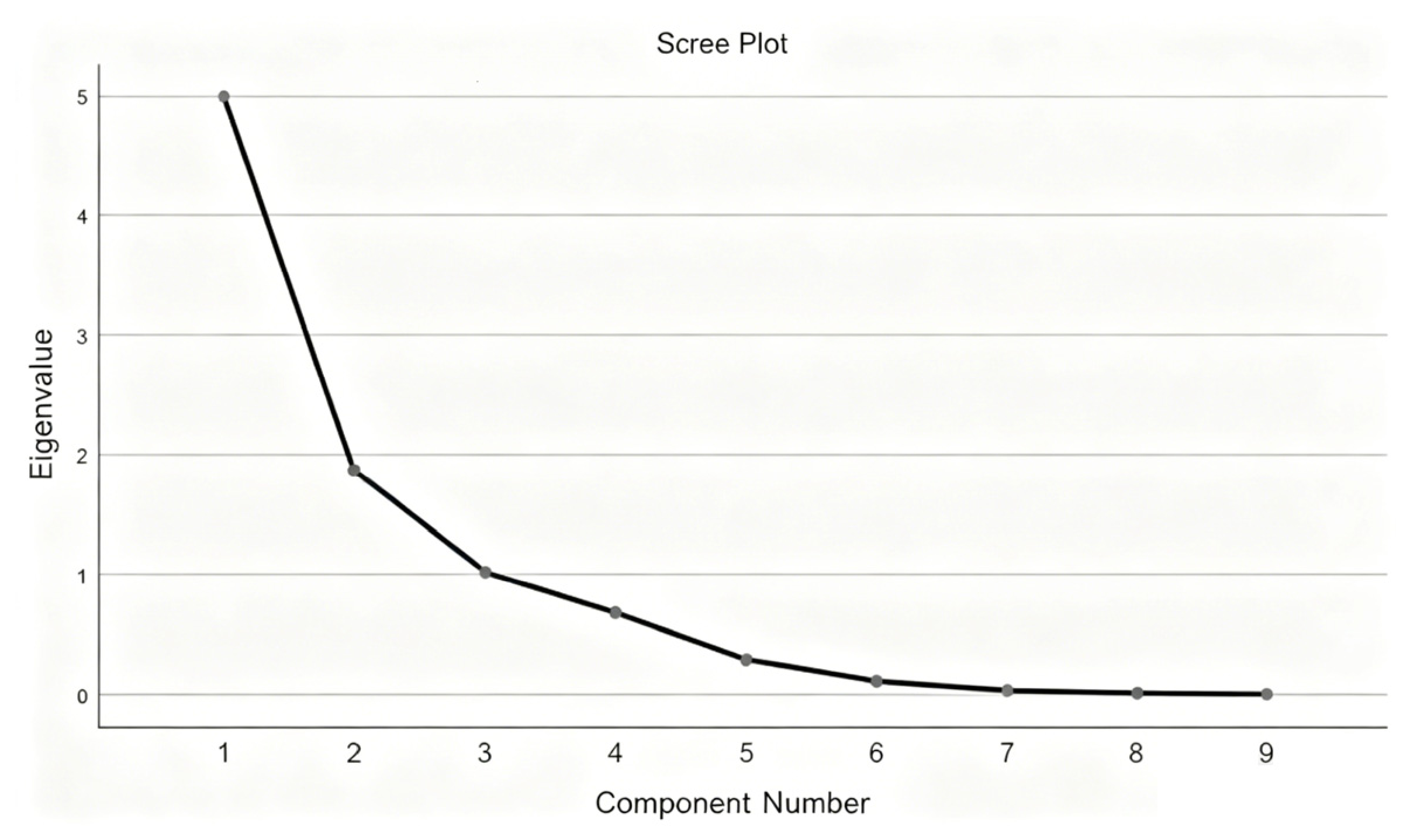
Figure 5 shows the scree plot of the factor analysis, which can be used to assist in determining the number of factors to extract. The inflection point where the scree plot changes abruptly from steep to flat indicates the reference number of factors to be extracted.
(4)
Communalities
Table 3 shows the communalities of the original variables under the initial solution (all equal to 1), as well as the extent to which they can be represented by the extracted factors (mostly above 75%). This indicates that little information is lost, each variable can be explained by the extracted factors, and the factor analysis achieves good results.
(5)
Total Variance Explained
Among the initial eigenvalues, three components have eigenvalues greater than 1 in the Total column, while the remaining components do not reach or exceed 1. In the Extraction Sums of Squared Loadings section, the three components with eigenvalues greater than 1 are listed separately. These three eigenvalues are arranged in descending order, so the first common factor explains the largest variance. In the Rotation Sums of Squared Loadings section, the information in the Total column changes slightly compared to that in the Extraction Sums of Squared Loadings section, but the difference is not significant.
According to Table 4, the number of factors extracted is three, based on initial eigenvalues greater than 1. By comparing the three factors before and after rotation, it is found that the variance contribution rates change after rotation, while the cumulative variance contribution rate remains unchanged at 87.411%, which is greater than 80%, indicating that the explanatory power of the factors is very good.
(6)
Component Matrix
Table 5 presents the component matrix. Compared with the rotated component matrix in Table 6, the factor implications become clearer. The first factor includes cumulative gradient mean, roughness, standard deviation and slope standard deviation; the second factor consists of kurtosis, correlation coefficient and skewness; the third factor covers skewness and information entropy. Table 7 shows the component transformation matrix.
Finally, the factor scores are saved as variables, and three new variables, “FAC1_1”, “FAC2_1”, and “FAC3_1”, are added. These three variables are regarded as the result of dimensionality reduction in the original variables. Through weighted calculation, the proportion of the variance contribution rate of each rotated factor to the total cumulative variance contribution rate is used as the weight for comprehensive evaluation.
Figure 6 shows the comprehensive evaluation results of the factor analysis. Compared with the gravity anomalies in Figure 2, it can be observed that in the central part of the sea area, the overall scores are relatively high. This aligns with the cliff-like decline in gravity anomalies in this region, indicating that sea areas with more dramatic gravity changes are more suitable for underwater gravity-matching navigation. In the southwestern sea area, although the gravity anomaly values are relatively high, the overall trend is relatively smooth with little fluctuation, resulting in weaker suitability.

4. TERCOM Algorithm

4.1. Basic Principles

The working principle of the TERCOM algorithm is as follows: When an underwater vehicle is located in a certain sea area, a gravity measurement terminal is used to obtain a gravity value profile along the track. The measured real-time profile is then correlated with the pre-stored reference map profile, and the geographical position of the vehicle is determined based on the best matching principle [23,24].
The calculation steps are as follows:
① Measured gravity profile. The gravity measurement terminal collects gravity values at certain intervals and, after correction calculations, obtains a sequence of gravity anomaly values. Considering that the marine gravity reference map has a resolution of 1′, the matching track length for each single match is set to be no less than 5000 m, and the measured gravity profile is extracted.
② Gravity profile extraction. After obtaining the measured gravity profile, a fixed-size sliding window of the gravity reference map is determined centered on the position output by the inertial navigation system. Within this sliding window, track sequences parallel to the position output by the inertial navigation system are selected, and the gravity reference map profile is extracted using interpolation methods.
③ Correlation test. A correlation operator is used to test the degree of correlation between each extracted gravity profile and the measured gravity profile. This paper adopts the Mean Square Difference (MSD) operator. That is, when the M S D t x , t y is minimized, the correlation is optimal, and the corresponding track point is the best matching position [25,26].
④ After obtaining the best matching position, the navigation system is corrected.

4.2. Algorithm Improvement

The traditional TERCOM algorithm neglects rotation and scale variations, which necessitates improvement. The calculation process is as follows:
① Obtain parallel tracks P ˜ i = 1 , 2 , 3 , … , m through translation, keeping the starting point of P ˜ i = 1 , 2 , 3 , … , m unchanged. Set the rotation angle between − ∂ , ∂ , with a step size of S , and perform m rotations of the angle transformation.
② Set the scale variation between − r , r , with a step size of t , and perform n scale transformations.
③ Apply the rotation angle and scale transformation coefficients to perform rotational and translational transformations on l parallel tracks P ˜ i = 1 , 2 , 3 , … , m , obtaining l × m × n trajectories.
④ Calculations are performed using Equation (33), and the position with the minimum mean squared deviation (MSD) is determined as the optimal matching position.
Considering that traversing all grid points incurs a large computational cost and reduces matching efficiency, a coarse matching process is adopted in practical calculations to obtain the initial trajectory. This initial trajectory is taken as the search starting point for fine matching, and the search range is further narrowed, accompanied by reduced step sizes for rotation and scaling variations. Fine matching calculation is then performed to obtain the optimal matching trajectory points.

4.3. Evaluation Indexes

In correlation analysis, normalized correlation coefficient (NPC), mean absolute difference (MAD), mean square deviation (MSD) and other operators can be selected as evaluation indexes. The relevant formulas are as follows.
M A D t x , t y = 1 N ∑ i = 1 N Δ g i x , y − Δ g ˜ i x + t x , y + t y
N P C t x , t y = ∑ i = 1 N Δ g i x , y ⋅ Δ g ˜ i x + t x , y + t y ∑ i = 1 N Δ g i x , y 2 ⋅ ∑ i = 1 N Δ g ˜ i x + t x , y + t y 2
M S D t x , t y = 1 N ∑ i = 1 N Δ g i x , y − Δ g ˜ i x + t x , y + t y 2
In the formula, Δ g i x , y represents the gravity anomaly values collected by the gravity measurement terminal, and Δ g ˜ i x + t x , y + t y represents the gravity profile extracted from the gravity reference map. t x , t y is the offset in longitude and latitude between the matched track and the corresponding real track point x , y . The optimal matching trajectory is determined by maximizing the NPC value and minimizing the MAD and MSD values. According to Reference [27], among the three operators, the normalized correlation exhibits the lowest accuracy. Under low signal-to-noise ratio conditions, the mean absolute difference achieves higher accuracy, while the mean square deviation shows superior accuracy in high signal-to-noise ratio environments.

4.4. Simulation Validation Results

The division of suitable areas is a 0-1 classification problem. A more direct method for evaluating the suitability of sliding windows is to conduct simulation experiments. A sliding window was used for validation, with a total of 2704 sliding windows. The starting point of the track is located at the lower-left corner of the sliding window. The starting point of the simulated pure inertial navigation track is offset 2 nautical miles north and 0 nautical miles east from the real track starting point. Each track contains a total of 13 sampling points, with a navigation speed set to 8 nautical miles/h. Other parameter settings for the inertial navigation system are referenced in Table 8.
The simulation parameters are comprehensively determined combined with the typical working conditions of underwater vehicles and the actual error characteristics in experiments, with specific descriptions as follows. A typical heading angle of 45° is selected for the track to simulate the common straight-line navigation condition underwater. Conducting experiments with different sliding windows can effectively improve the generalization verification capability of algorithms and models. As the core error source of inertial navigation, gyroscope drift is set with a constant drift of 0.05°/h and a random drift of 0.01°/h by referring to the conventional error indicators of medium- and low-precision shipborne/underwater inertial measurement components, which conforms to the actual error level of civil underwater navigation equipment. The error parameters of the accelerometer are determined based on the factory error range of inertial sensors and the long-term bias stability characteristics during operation, with a bias of 1 × 10 − 4   g and a random bias of 5 × 10 − 5   g , which is consistent with the error evolution law of inertial devices in complex underwater environments. Considering the cumulative error characteristics of inertial navigation during long-distance underwater navigation, the random error of INS indicated track and real simulated track are set to 0.12   n   m i l e and 0.06   n   m i l e respectively, basically matching the error accumulation characteristics of conventional autonomous inertial positioning. Underwater gravity measurement is affected by instrumental noise, marine environmental disturbance, measurement sampling interference and other factors. Referring to the conventional measurement accuracy of marine gravity measurement systems, the root mean square error of gravity anomaly is set to 1   m G a l , which is in line with the error distribution law of measured gravity data.
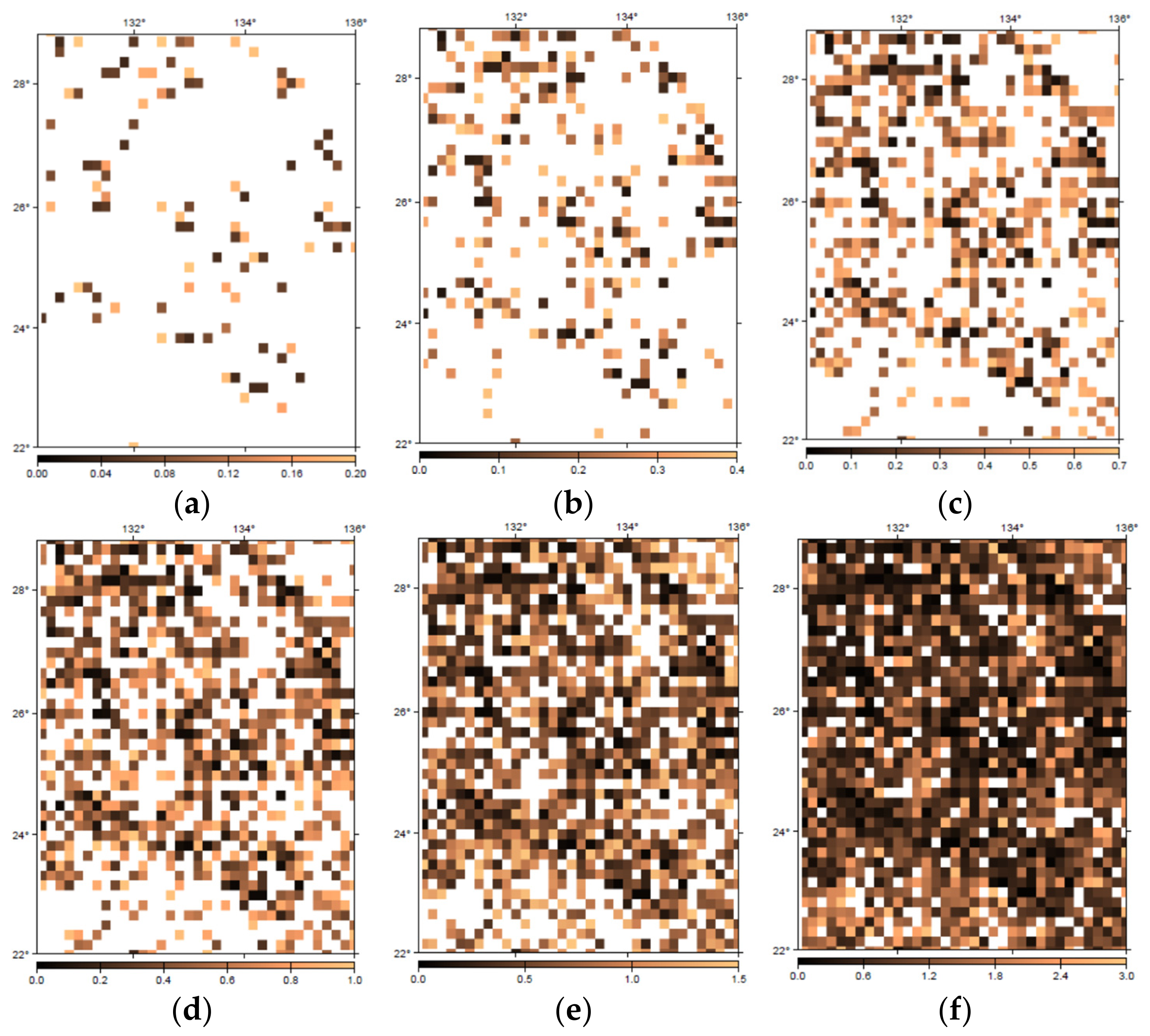
Using the improved TERCOM algorithm, the standard deviation of the position difference between the matched track points and the corresponding real track points was obtained. To more intuitively display the matching navigation effects of different sliding windows, a standard deviation of the difference greater than 1 nautical mile is considered a matching failure, while less than 1 nautical mile is considered a successful match. Figure 6 shows the distribution of sliding windows when the standard deviation of the difference is less than 0.2 nautical miles, 0.4 nautical miles, 0.7 nautical miles, 1.0 nautical miles, 1.5 nautical miles, and 3 nautical miles, respectively. The white areas represent the distribution of sliding windows that exceed their respective standard deviations.

5. Limitations of Statistical Methods

It can be observed that: ① Compared with the comprehensive scores of the factor analysis, most of the sliding windows with a standard deviation of less than 0.2 nautical miles in Figure 7a are distributed in sea areas with high comprehensive scores. In areas with low comprehensive scores, such as the southwestern sea area, there are no such high-precision matching cases. ② As the standard deviation of the difference increases, the overall trend of the sliding window distribution changes. The factor analysis method can reflect the suitability performance of the sliding windows. Areas with high comprehensive scores have a higher probability of successful matching, while areas with low comprehensive scores have a slightly lower probability of success. ③ In Figure 7e, the sea areas with a standard deviation greater than 3 nautical miles appear blank, indicating that the matching performance in these areas is generally poor. This is consistent with the low comprehensive scores of these areas in the factor analysis. It is necessary to explore underwater navigation methods suitable for non-suitable areas to effectively fill the technical gap.
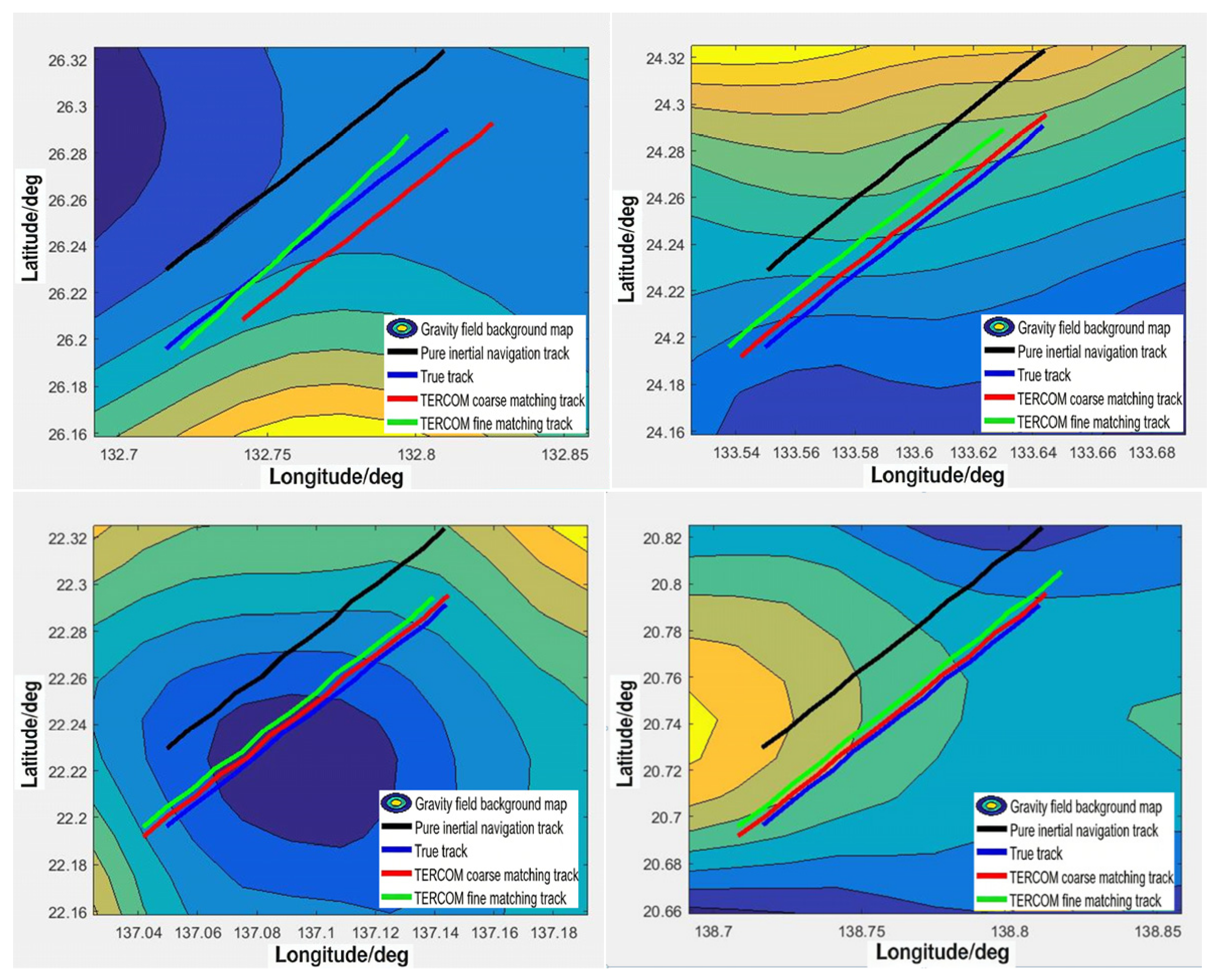
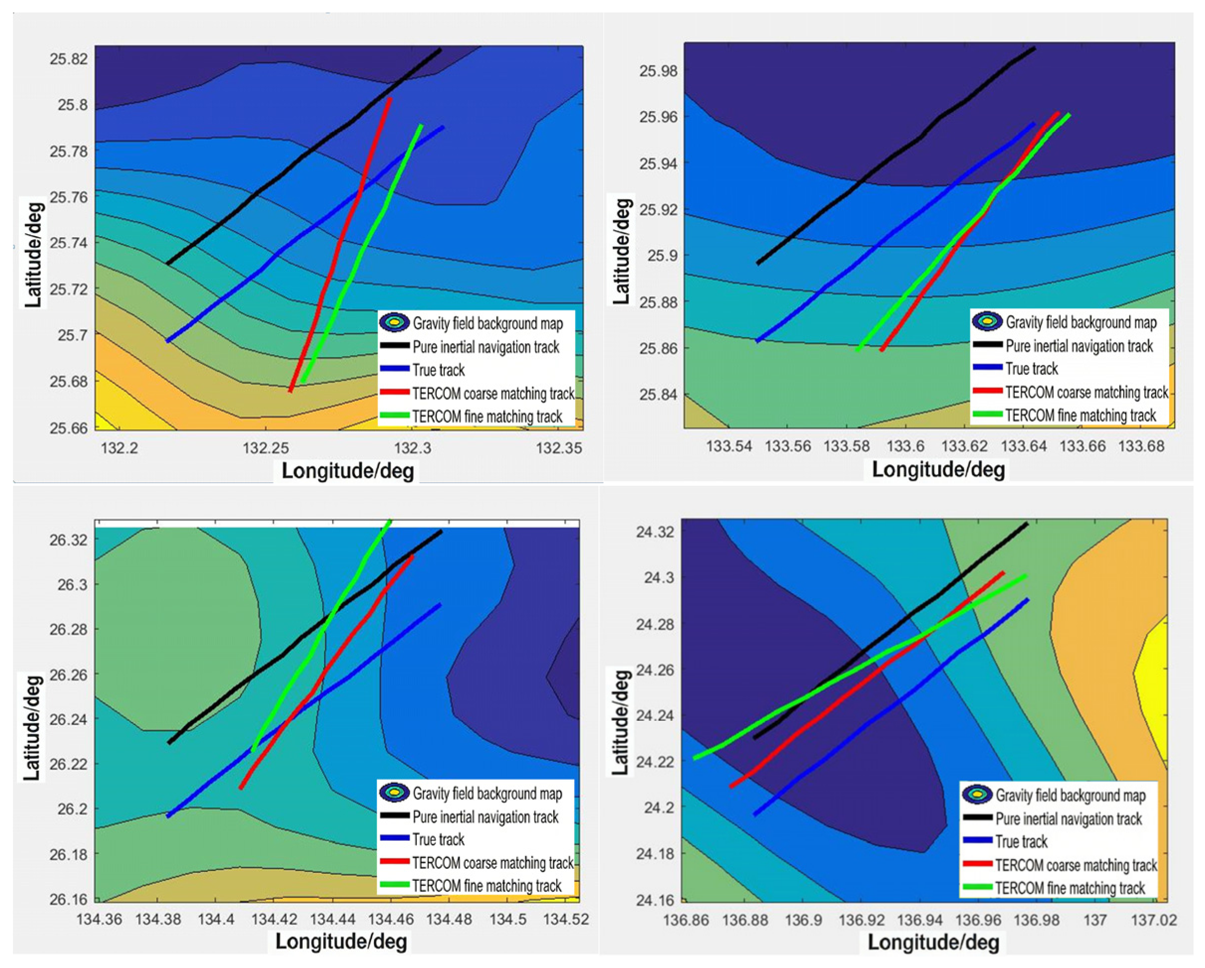
Statistical methods, such as factor analysis, require setting a threshold as the basis for evaluating navigation suitability. Each sliding window in the experimental sea area is verified by simulation using the TERCOM algorithm. The consistency between the adaptable and inadaptable areas divided by factor analysis under different thresholds and the simulation results is compared. The best consistency is achieved at a threshold of −0.2; therefore, the threshold is set to −0.2 in this study. Sliding windows with scores above this threshold are considered suitable for matching navigation, while those below are considered unsuitable. Eight sliding windows were selected, and the threshold classification results were compared with the simulation verification results of the TERCOM algorithm, as shown in Figure 8 and Figure 9. Although some windows scored above the −0.2 threshold, they failed in the simulation experiments. Conversely, some windows scored below the −0.2 threshold but succeeded in the simulation experiments. Table 9 shows the statistical information of the matching results for these eight windows. Figure 8 illustrates the navigation verification results for four sliding windows with comprehensive scores below −0.2 (Nos. 796, 1068, 2172, and 2701), all of which achieved good matching results. Figure 9 shows the results for four sliding windows with comprehensive scores above −0.2 (Nos. 643, 1058, 1316, and 2108), all of which failed in matching.
Conclusions: ① The suitability of sliding windows is influenced by multiple factors. The factor analysis method of characteristic parameters can reflect the suitability performance of sliding windows to a certain extent. ② A more accurate determination of suitability can be verified through simulation experiments. ③ No statistical relationship can be established between the nine characteristic parameters and the simulation results. It is necessary to introduce intelligent learning algorithms to classify and evaluate suitability.

6. Optimized Classification

6.1. Learning Vector Quantization Neural Network Algorithm

The LVQ-1 network consists of three layers: input layer, competitive layer (core layer), and output layer. The functions, structural parameters, and connection methods of each layer are described as follows.

6.1.1. Input Layer

The core function of the input layer is to receive multi-dimensional evaluation features of the gravity datum adaptation zone, convert them into feature vectors of a unified dimension, and serve as the input signals of the network. The number of nodes strictly corresponds to the dimension of the evaluation features to ensure the complete transmission of feature information.
Number of nodes: Denoted as n, corresponding to the n core feature indicators for gravity datum adaptation zone evaluation.
Input vector: Defined as X = [ x 1 , x 2 , . . . , x n ] T , where x i ( i = 1,2 , . . . , n ) is the normalized value of the i-th evaluation feature. Due to the large differences in units (dimensions) among gravity feature indicators, normalization is essential to ensure the balanced contribution of each feature to network training.
Data preprocessing: All input features are mapped to the interval [ 0,1 ] using the Min-Max normalization method to eliminate the influence of dimensions. The formula is
x i ′ = x i − m i n ( x i ) m a x ( x i ) − m i n ( x i )
where x i is the original feature value, x i ′ is the normalized value, and m i n ( x i ) and m a x ( x i ) are the minimum and maximum values of the feature, respectively.
Meanwhile, missing values are handled by mean filling or linear interpolation, and outliers are removed using the 3σ criterion to ensure the integrity and accuracy of input data.

6.1.2. Competitive Layer (Core Layer)

The competitive layer is the core of the LVQ network, also known as the “vector quantization layer”. It is responsible for clustering and competitive selection of input feature vectors. By calculating the similarity between the input vector and the weight vectors of the competitive layer, the “winning neuron” is determined to achieve preliminary feature classification. Its number of nodes is closely related to the number of adaptation zone grades and sample distribution.
Number of nodes: Denoted as m, which is an integer multiple of the number of adaptation zone grades (recommended m = k × t , where k is the number of adaptation zone grades and t is the number of “prototype vectors” corresponding to each grade, t ≥ 2 ). Combined with common scenarios of gravity datum adaptation zone evaluation (three grades: high adaptation, medium adaptation, low adaptation), m = 6 ∼ 12 is recommended (i.e., 2~4 prototype vectors per grade). A larger number of prototype vectors enhances the model’s adaptability to complex gravity features but increases the computational cost accordingly.
Weight vector: Each neuron in the competitive layer corresponds to a weight vector W j = [ w j 1 , w j 2 , . . . , w j n ] T ( j = 1,2 , . . . , m ). The dimension of the weight vector is consistent with that of the input vector (both are n-dimensional), and its physical meaning is the “feature prototype of a certain adaptation zone grade”. The core of the training process is to continuously adjust the weight vectors to approximate the sample feature centers of the corresponding grades.
Competition mechanism: The minimum distance competition strategy is adopted. The Euclidean distance between the input vector X and each weight vector W j of the competitive layer is calculated, and the neuron with the smallest distance is the “winning neuron”. The formula is
d j = ∑ i = 1 n ( x i − w j i ) 2 ( j = 1,2 , . . . , m )
The winning neuron is responsible for the preliminary classification of the input sample, and its corresponding class label is the prototype of the predicted class of the sample.
Class mapping: A fixed class label (corresponding to adaptation zone grades, e.g., high adaptation, medium adaptation, low adaptation) is assigned to each competitive layer neuron. Multiple competitive layer neurons (i.e., multiple prototype vectors) correspond to the same adaptation zone grade to ensure the model can cover different gravity feature variations under that grade.

6.1.3. Output Layer

The output layer is responsible for converting the competitive results of the competitive layer into clear gravity datum adaptation zone evaluation results (adaptation zone grades). The number of nodes strictly corresponds to the number of adaptation zone grades, and the output form is concise for subsequent result analysis and verification.
Number of nodes: Denoted as k, corresponding to k adaptation zone grades. According to the actual requirements of gravity navigation, k = 3 is recommended (high-adaptation zone, medium-adaptation zone, low-adaptation zone); for more refined evaluation, k = 4 can be set by adding a “non-adaptation zone”.
Output form: Adopts One-Hot encoding, i.e., the output vector is a k-dimensional binary vector, where only the position corresponding to the adaptation zone grade is 1 and the rest are 0 (e.g., high-adaptation zone outputs [ 1,0 , 0 ] , medium-adaptation zone outputs [ 0,1 , 0 ] ), facilitating classification error calculation and confusion matrix plotting.
Output logic: Maps the class label of the winning neuron in the competitive layer to the encoded vector of the output layer. If the label of the winning neuron is “high adaptation”, the corresponding node for high adaptation in the output layer is set to 1 and the others to 0. In case of a tie (equal distance) among multiple neurons, the grade with the highest frequency of class labels is selected as the output result.

6.1.4. Program Steps

Step 1: Initialize parameters. Determine the number of input layer nodes n , competitive layer nodes m , and output layer nodes k ; set the initial learning rate η , learning rate decay coefficient α , initial neighborhood radius σ , and maximum training iterations E . Adopt the sample center initialization method to determine the initial weight vectors W j of each neuron in the competitive layer, and assign a corresponding adaptation zone grade label to each competitive layer neuron.
Step 2: Input training samples. Randomly select a normalized sample input vector X from the training set, and record the true label t (adaptation zone grade) of the sample.
Step 3: Compete to select the winning neuron. Calculate the Euclidean distance d j between the input vector X and all weight vectors W j of the competitive layer, and select the neuron with the minimum distance as the winning neuron, denoted as j * , with its corresponding class label t * .
Step 4: Update weight vectors. Update the weight vectors of the winning neuron and its neighboring neurons according to the consistency between the label of the winning neuron and the true label of the sample, with the update rules as follows:
Where η ( t ) is the learning rate at the t -th iteration, η ( t ) = η 0 × α t ; neurons within the neighborhood are selected based on the neighborhood radius σ ( t ) = σ 0 × α t , and neurons with a distance from the winning neuron index ≤ σ ( t ) are defined as neighboring neurons.
If t * = t (correct classification), the weights of the winning neuron and its neighboring neurons move closer to the input vector, and the update formula is W j ( t + 1 ) = W j ( t ) + η ( t ) × [ X − W j ( t ) ] ( j represents the winning neuron and its neighboring neurons);
If t * ≠ t (incorrect classification), the weight of the winning neuron moves away from the input vector, and the update formula is W j * ( t + 1 ) = W j * ( t ) − η ( t ) × [ X − W j * ( t ) ] (only update the winning neuron, no updates for neighboring neurons).
Step 5: Iterative training. Repeat Steps 2 to 4, traverse all samples in the training set to complete one iteration; calculate the classification accuracy of the validation set every 10 iterations, and record the validation set error.
Step 6: Terminate training. Stop training when any of the following conditions is met: ① the maximum training iterations E are reached; ② the validation set accuracy does not improve for 10 consecutive iterations (the error variation is less than 10 − 4 ); ③ the validation set accuracy reaches a preset threshold (e.g., ≥ 90 ). After training termination, save the optimal model parameters (competitive layer weight vectors, class label mapping relationship, normalization parameters).

6.2. Extreme Learning Machine

Combined with the characteristic parameters of the gravity reference map, a single hidden layer feedforward ELM network structure is designed, which consists of three layers: the input layer, the hidden layer, and the output layer. The functions and structural parameters of each layer are specified as follows.

6.2.1. Input Layer

The core function of the input layer is to receive multi-type characteristic parameters of the gravity reference map as the input vector of the model, and its number of nodes is consistent with the dimension of evaluation features.
Number of nodes: Defined as n , corresponding to n core characteristic indicators for the evaluation of gravity reference matching areas.
Input vector: Defined as X = [ x 1 , x 2 , . . . , x n ] T , where x i ( i = 1,2 , . . . , n ) represents the normalized value of the i -th evaluation feature.
Data preprocessing: All input features are mapped to the interval [ 0,1 ] using the Min-Max normalization method. The formula is x i ′ = x i − m i n ( x i ) m a x ( x i ) − m i n ( x i ) . In the formula, x i is the original feature value, x i ′ is the normalized value, and m i n ( x i ) and m a x ( x i ) denote the minimum and maximum values of the corresponding feature, respectively.

6.2.2. Hidden Layer

As the core of the ELM model, the hidden layer performs nonlinear mapping on input features. The number of hidden layer nodes directly affects the generalization ability and training accuracy of the model. Excess nodes will lead to overfitting, while insufficient nodes will cause underfitting.
Number of nodes: Defined as L , determined by the combination of empirical value selection and cross-validation optimization. The initial value range is set to [ 10,100 ] , and the optimal number of hidden layer nodes is finally selected through K-fold cross-validation.
Activation function: Nonlinear activation functions suitable for regression and classification tasks are selected. Combined with the quantitative requirements for gravity reference matching area evaluation (matching score regression or matching-level classification), one of the following two activation functions is recommended, and the optimal one can be selected through experimental comparison:
Sigmoid function: g ( x ) = 1 1 + e − x . It is applicable to classification tasks such as matching-level division (high, medium and low matching areas), with an output range of [ 0,1 ] , which facilitates probabilistic judgment.
ReLU function: g ( x ) = m a x ( 0 , x ) . It is applicable to regression tasks such as quantitative calculation of matching scores. It can solve the problem of gradient vanishing and accelerate training speed, and is suitable for large sample datasets.
Weights and biases: The connection weight matrix W (dimension: L × n ) from the input layer to the hidden layer and the hidden layer bias vector b (dimension: L × 1 ) are randomly generated within the range of [ − 1,1 ] without iterative adjustment, which conforms to the core characteristics of ELM, i.e., random initialization and rapid training.
Hidden layer output: Defined as H (dimension N × L , where N is the number of samples), calculated as H = g ( W X + b ) . Here, g ( · ) represents the hidden layer activation function, and batch matrix operation is adopted to improve training efficiency.

6.2.3. Output Layer

The output layer converts the nonlinear mapping results of the hidden layer into evaluation results of gravity reference matching areas, and the number of nodes is determined by the type of evaluation tasks.
Number of nodes:
Classification task: Set as k , corresponding to k matching area levels (e.g., k = 3 for high, medium and low matching areas). The output adopts One-Hot encoding to facilitate classification error calculation.
Regression task: Set as 1 for quantitative evaluation of matching scores, and the output is the matching score within the range of [ 0,1 ] , which directly reflects the regional matching degree.
Output layer weight: Defined as β (dimension: L × k or L × 1 ), solved by the least square method to minimize the sum of squares of output errors. The solving formula is β = H † T , where H † is the Moore–Penrose generalized inverse of the hidden layer output matrix H , and T is the sample label matrix (dimension: N × k or N × 1 ).
Output result: Defined as Y (dimension: N × k or N × 1 ) and calculated as Y = H β . For classification tasks, the output is converted into probability values through the Softmax function; for regression tasks, the matching score is directly output.

6.2.4. Experimental Procedures

Step 1: Environment Setup. Install Python 3.13 and relevant core libraries, implement the extreme learning machine (ELM) algorithm code, and set random seeds for reproducibility.
Step 2: Data Loading and Preprocessing. Load experimental data, conduct data cleaning, normalization, and dataset splitting, then save the preprocessed data files.
Step 3: ELM Model Initialization. Define candidate sets for the number of hidden layer nodes L, activation functions (Sigmoid, ReLU, tanh), and regularization parameter λ.
Step 4: Model Training and Parameter Optimization. Adopt 5-fold cross-validation, traverse all parameter combinations to train the ELM model, record the validation set error corresponding to each parameter group, and select the parameter combination with the optimal validation set error.
Step 5: Model Testing. Apply the ELM model with the optimal parameter combination to the test set, calculate test set performance metrics, record test results, and plot the confusion matrix or fitting curve.
Step 6: Stability Verification. Repeat Steps 3 to 5 with different random seeds (e.g., 42, 100, 200) for three independent repeated experiments, compute the mean and standard deviation of each performance metric, and verify the stability of the model.
Step 7: Comparative Experiment. Conduct a comparison with the learning vector quantization (LVQ) algorithm using the same dataset and performance metrics, and validate the advantages of the ELM algorithm in the evaluation of gravity datum adaptation zones.

6.3. Calculation and Analysis

The extreme learning machine and learning vector quantization neural network algorithms are used for classification calculations. In total, 7/8 of the windows in the calculation sea area are selected to form the training set as the input of the network, and the suitability evaluation results of different windows obtained through simulation verification methods are used as the training output. The training set data is used to train the above two intelligent algorithms, and the remaining 1/8 of the windows, used as the test set data, are utilized to verify the classification results.
Designed in accordance with method requirements, the implementation steps shown in Figure 10 consist of four parts:
Step 1: Generation of Test Set and Training Set
The dataset for the calculated sea area includes a total of 2366 windows, of which 1058 are suitable windows and 1308 are unsuitable windows. The training set comprises a total of 338 windows, including 158 suitable windows and 180 unsuitable windows.
The input data for each window includes 14 parameters: Tk1, Tk2, Tk3, Tk4, Tk5, Tk6, standard deviation, roughness, information entropy, correlation coefficient, kurtosis coefficient, skewness coefficient, standard deviation of slope, and cumulative gradient mean.
Step 2: Creation and Training of Neural Network/Extreme Learning Machine
After the data preparation is completed, relevant functions are used to construct the neural network or extreme learning machine. Parameters can be set and modified if necessary.
Step 3: Simulation Testing
After training, the two intelligent algorithms are used to perform validation calculations on the test set data, obtaining corresponding outputs and classifications.
Step 4: Performance Evaluation
To objectively evaluate the classification performance of the two intelligent algorithms, the confusion matrix, precision, recall, F1-score and accuracy are adopted as the core evaluation indicators. The definition, calculation method and adaptability to the two algorithms of each indicator are described as follows. All indicators range from 0 to 1, and a value closer to 1 indicates better classification performance of the algorithm.
①
Confusion Matrix
A confusion matrix is a matrix form that intuitively reflects the classification results of an algorithm. It quantifies the classification errors of the model for each category by counting the correspondence between the predicted categories and the true categories of samples, and provides a basis for the calculation of accuracy indicators. This paper defines the confusion matrix based on binary classification tasks. For multi-class classification tasks, they can be decomposed into multiple binary classification tasks through one-vs-one or one-vs-rest strategies, with the core logic of the confusion matrix remaining consistent.
In binary classification tasks, the confusion matrix is a 2 × 2 dimensional matrix. As shown in the Table 10, rows represent the true sample categories, and columns represent the algorithm-predicted categories:
②
Accuracy
Accuracy is the most intuitive overall evaluation metric for classification performance. It is defined as the proportion of correctly classified samples to the total number of samples, reflecting the model’s overall classification capability. Its calculation formula is as follows:
A c c = T P + T N T P + T N + F P + F N
Adaptability Description: Accuracy is applicable to scenarios with balanced sample category distribution.
③
Recall
Also known as sensitivity, recall refers to the proportion of truly positive samples that are correctly predicted as positive. It measures the recognition ability for positive samples and focuses on reducing missed detection (FN). Its calculation formula is as follows:
R e c a l l = T P T P + F N
Adaptability Description: Recall is suitable for scenarios with high missed detection costs, such as anomaly monitoring and target recognition.
The error between the predicted values and the true values is calculated to evaluate the classification capability of the models. Meanwhile, the computational efficiency of different intelligent algorithms is compared.
Table 11 shows the performance evaluation results and computation times of different intelligent algorithms. Windows that are successfully matched in the simulation verification are considered suitable areas, while others are considered unsuitable areas. There are a total of 1216 suitable areas and 1488 unsuitable areas. In the training set, there are 1058 suitable areas and 1308 unsuitable areas. In the test set, there are 158 suitable areas and 180 unsuitable areas. From the results obtained by the two intelligent algorithms in Table 11, it can be seen that in terms of accuracy, ELM delivers stronger generalization performance, achieving an accuracy of over 95% on the dataset, which is significantly better than LVQ. Limited by the update mechanism of prototype vectors, LVQ exhibits weak recognition capability for boundary positive samples, with a recall rate of approximately 88%. By contrast, ELM possesses superior nonlinear mapping ability in the hidden layer, enabling it to effectively capture the features of positive samples and reach a recall rate of 94% with a lower missed detection rate. The extreme learning machine outperforms the learning vector quantization neural network algorithm in terms of both classification accuracy and timeliness.

7. Conclusions

For long-endurance underwater vehicles using gravity-matching navigation, it is necessary to evaluate the suitability of the gravity reference map to reasonably plan navigation paths and avoid adverse effects such as non-suitable areas, seamounts, and underwater obstacles. The main research contents are as follows:
(1)
A factor analysis method is proposed to comprehensively evaluate nine characteristic parameters. Calculation formulas for nine characteristic parameters, including standard deviation and absolute roughness convolution, kurtosis coefficient, skewness coefficient, standard deviation, roughness, cumulative gradient, information entropy, correlation coefficient, and standard deviation of slope, are provided. A specific area in the Pacific Ocean is taken as the research object, and the sliding window method is used to obtain the characteristic parameter values. To address the inaccuracy of suitability evaluation using a single parameter, the statistical method of factor analysis is adopted. Variables are grouped based on the magnitude of correlations, and comprehensive evaluation values are obtained.
(2)
The TERCOM algorithm is used to verify the suitability of the sliding windows. Simulation tracks are designed for 2704 sliding windows in the study area, and the improved TERCOM algorithm is used for matching calculations. Compared with the comprehensive scores of factor analysis (with a threshold set at −0.2), some sliding windows exhibit inconsistencies between simulation verification results and comprehensive feature results, demonstrating the limitations of statistical methods in suitability evaluation.
(3)
Given that no statistical relationship can be established between some simulation verification results and the nine characteristic parameters, two intelligent algorithms, the learning vector quantization neural network algorithm and the extreme learning machine, are considered for automatic classification and evaluation of suitability. The results show that both intelligent algorithms successfully achieve classification calculations. In terms of computational efficiency and classification accuracy, the extreme learning machine outperforms the learning vector quantization neural network algorithm.

Author Contributions

Conceptualization, M.O.; methodology, M.O.; software, M.O. and Z.Z.; validation, X.N. and Y.Z.; formal analysis, X.N., M.O. and H.H.; investigation, M.O. and Z.Z.; resources, H.H.; writing—original draft preparation, Y.Z. and H.H.; writing—review and editing, X.N., H.H. and M.O.; visualization, B.G., Y.Z. and Z.Z.; funding acquisition, M.O. All authors have read and agreed to the published version of the manuscript.

Funding

This research was funded by National Natural Science Foundation of China (grant number 42388102 and 42174001) and Open fund of State Key Laboratory of Spatial Datum (SKLGIE2024-ZZ-1). The APC was funded by SKLGIE2024-ZZ-1.

Data Availability Statement

The raw data supporting the conclusions of this article will be made available by the authors on request.

Acknowledgments

Authors acknowledge the support of the State Key Laboratory of Spatial Datum, Xi’an Research Institute of Surveying and Mapping.

Conflicts of Interest

The authors declare no conflicts of interest.

References

  1. Wang, B.; Zhu, Y.; Deng, Z.; Fu, M. The gravity matching area selection criteria for underwater gravity-aided navigation ap-plication based on the comprehensive characteristic parameter. IEEE/ASME Trans. Mechatron. 2016, 21, 2935–2943. [Google Scholar] [CrossRef] [Scilit]
  2. Yang, Y.; Xu, T.; Xue, S. Research Progress and Prospect of Marine Geodetic Datum and Marine Navigation Technology in China. Acta Geod. Cartogr. Sin. 2017, 46, 1–8. [Google Scholar]
  3. Li, K.H.; Xiong, L.; Cheng, L.; Ma, J. The research of matching area selection criterion for gravity gradient aided navigation. In Proceedings of the Pattern Recognition: 6th Chinese Conference, CCPR 2014, Changsha, China, 17–19 November 2014. [Google Scholar]
  4. Xiong, L.; Li, K.; Tang, J.; Ma, J. Research on matching area selection criteria for gravity gradient navigation based on principal component analysis and analytic hierarchy process. In MIPPR 2015: Remote Sensing Image Processing, Geographic Information Systems, and Other Applications; SPIE: Bellingham, WA, USA, 2015; Volume 9815, pp. 287–294. [Google Scholar]
  5. Xiao, Y.; Zhang, J.; Cao, J.; Chen, K.; Wang, Y.; Hong, X. Suitability Analysis of Gravity Matching Navigation Based on Multi-Attribute Decision Making Theory. Geomat. Inf. Sci. Wuhan Univ. 2023, 48, 1089–1099. [Google Scholar]
  6. Liu, F.; Li, F.; Jing, X. Navigability analysis of local gravity map with projection pursuit-based selection method by using gravitation field algorithm. IEEE Access 2019, 7, 75873–75889. [Google Scholar] [CrossRef] [Scilit]
  7. Wang, H.; Wu, L.; Chai, H.; Xiao, Y.; Hsu, H.; Wang, Y. Characteristics of marine gravity anomaly reference maps and accuracy analysis of gravity matching-aided navigation. Sensors 2017, 17, 1851. [Google Scholar] [CrossRef] [Scilit] [PubMed]
  8. Wu, L.; Wang, H.; Chai, H.; Zhang, L.; Hsu, H.; Wang, Y. Analysis and selection of global marine gravity/gravity gradient aided navigation matching areas. In China Satellite Navigation Conference (CSNC) 2018 Proceedings: Volume III; Springer: Singapore, 2018; pp. 887–895. [Google Scholar]
  9. Wang, B.; Zhou, M.; Deng, Z.; Fu, M. Sum vector-difference-based matching area selection method for underwater gravity-aided navigation. IEEE Access 2019, 7, 123616–123624. [Google Scholar] [CrossRef] [Scilit]
  10. Wang, C.; Wang, B.; Deng, Z.; Fu, M. A delaunay triangulation-based matching area selection algorithm for underwater gravity-aided inertial navigation. IEEE/ASME Trans. Mechatron. 2020, 26, 908–917. [Google Scholar] [CrossRef] [Scilit]
  11. Wang, C.; Wang, B.; Deng, Z.; Fu, M. A co-occurrence matrix-based matching area selection algorithm for underwater gravity-aided inertial navigation. IET Radar Sonar Navig. 2021, 15, 250–260. [Google Scholar] [CrossRef] [Scilit]
  12. Wang, S.; Zheng, W.; Li, Z. Optimizing matching area for underwater gravity-aided inertial navigation based on the convolution slop parameter-support vector machine combined method. Remote Sens. 2021, 13, 3940. [Google Scholar] [CrossRef] [Scilit]
  13. Zhao, M.; Xu, Z.; Ma, W. Analysis of terrain navigability in underwater terrain aided navigation. J. Phys. Conf. Ser. 2021, 1887, 012001. [Google Scholar] [CrossRef] [Scilit]
  14. Wang, B.; Li, T.; Deng, Z.; Fu, M. Wavelet Transform Based Morphological Matching Area Selection for Underwater Gravity Gradient-Aided Navigation. IEEE Trans. Veh. Technol. 2022, 72, 3015–3024. [Google Scholar] [CrossRef] [Scilit]
  15. Wang, B.; Cai, T.; Fang, K. The Quantification Method of Matching Capability of Areas in Gravity-Aided Inertial Navigation. IEEE Sens. J. 2022, 22, 20958–20967. [Google Scholar] [CrossRef] [Scilit]
  16. Zhao, X.; Zheng, W.; Xu, K.; Zhang, H. Optimizing the Matching Area for Underwater Gravity Matching Navigation Based on a New Gravity Field Feature Parameters Selection Method. Remote Sens. 2024, 16, 2202. [Google Scholar] [CrossRef] [Scilit]
  17. Mao, G.; Wu, L.; Xi, M.; Liu, S.; Xiong, C.; Bao, L.; Wang, Y. Algorithm for Selecting Adaptation Areas for Gravity Matching Navigation Based on Gravitational Deep Perception Model. Geomat. Inf. Sci. Wuhan Univ. 2024, 49, 2122–2144. [Google Scholar]
  18. Wang, M.; Zheng, W.; Zhao, S.; Li, X.; He, C. A Novel Curvature Directional Feature-Based Matching Area Clustering Method for Underwater Gravity-Aided Navigation. IEEE Trans. Instrum. Meas. 2025, 74, 1. [Google Scholar] [CrossRef] [Scilit]
  19. Zhang, W.; Wang, Y.; Zhao, S.; Deng, Z. A Gravity Matching Adaptability Analysis Method based on Gravity Directional Characteristics. IEEE Sens. J. 2026, 26, 1. [Google Scholar] [CrossRef] [Scilit]
  20. Ma, Y.; Ouyang, Y.; Huang, M.; Deng, K.; Qu, Z. Selection Method of Suitable Area Based on Information Entropy of Gravity Field Characteristic Parameters. J. Chin. Inert. Technol. 2016, 24, 763–768. [Google Scholar]
  21. Li, D.; Fan, R.; Wang, C.; He, Y.J.; Ren, W. Application of Factor Analysis Method in Suitability Analysis of Geo-magnetic Map. J. Navig. Position. 2022, 10, 121–129. [Google Scholar]
  22. Wang, C. Research on Key Technologies of Geomagnetic Aided Navigation. Master’s Thesis, Liaoning Technical University, Fuxin, China, 2022. [Google Scholar]
  23. Han, Y.; Wang, B.; Deng, Z.; Fu, M. An improved TERCOM-based algorithm for gravity-aided navigation. IEEE Sens. J. 2016, 16, 2537–2544. [Google Scholar] [CrossRef] [Scilit]
  24. Wei, E.; Dong, C.; Liu, J.; Tang, S. An improved TERCOM algorithm for gravity-aided inertial navigation system. J. Geomat. 2017, 42, 29–31. [Google Scholar]
  25. Ouyang, M. Comparison of TERCOM Algorithm and ICCP Algorithm for Underwater Matching Navigation. J. Geomat. Sci. Technol. 2020, 37, 350–355. [Google Scholar]
  26. Zou, J.; Xiao, Y.; Sun, A.; Wei, J.; Meng, N.; Ai, S. Joint Gravity Matching Navigation Using TERCOM and ICCP. J. Navig. Position. 2021, 8, 115–124. [Google Scholar]
  27. Yan, L.; Cui, C.; Wu, H. Gravity Matching Based on TERCOM Algorithm. Geomat. Inf. Sci. Wuhan Univ. 2009, 34, 261–264. [Google Scholar]
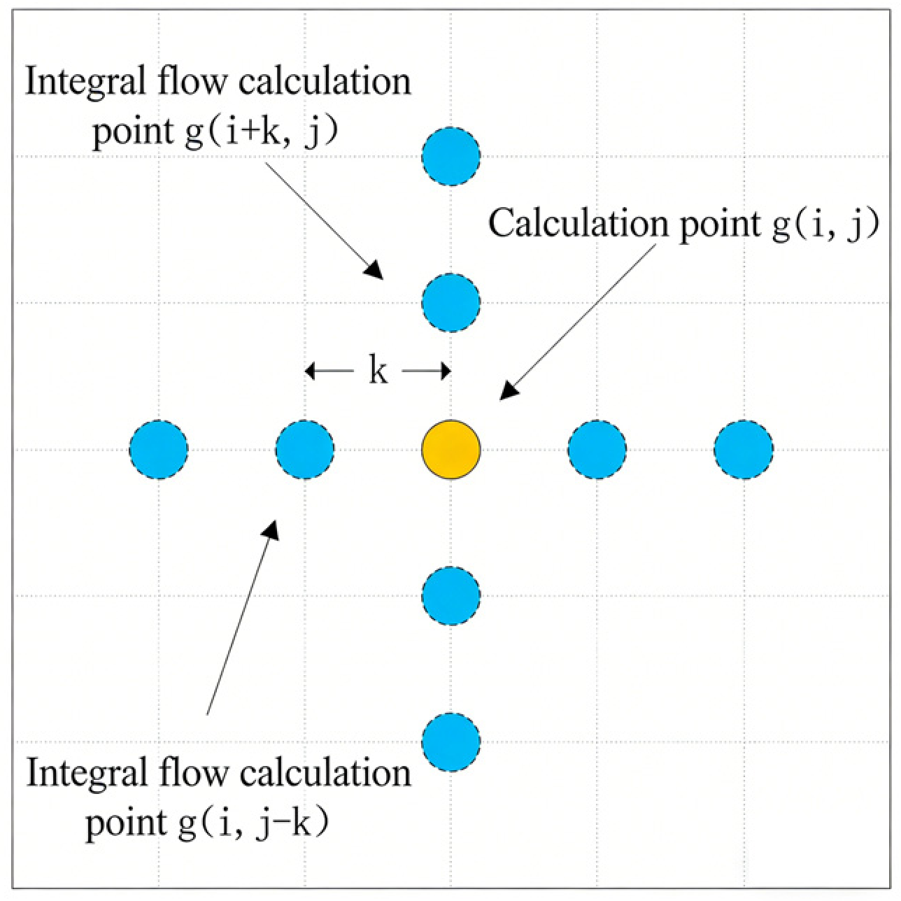
Figure 1. Schematic diagram of convolution parameters.
Remotesensing 18 02812 g001
Figure 2. Gravity anomaly in the study area.
Remotesensing 18 02812 g002
Figure 3. Gravity anomaly convolution characteristic parameter maps, (a–f) show the parameter values obtained through convolution operations when Γ is assigned values from 1 to 6.
Remotesensing 18 02812 g003
Figure 4. Characteristic parameter maps, from top to bottom and left to right, are (a) roughness, (b) standard deviation map of gravity anomaly, (c) kurtosis coefficient, (d) information entropy, (e) cumulative gradient mean map, (f) skewness coefficient, (g) standard deviation of slope, (h) correlation coefficient.
Remotesensing 18 02812 g004
Figure 5. Scree plot.
Remotesensing 18 02812 g005
Figure 6. Comprehensive scores.
Remotesensing 18 02812 g006
Figure 7. Distribution of sliding windows when the standard deviation of the difference is less than (a) 0.2 nm, (b) 0.4 nm, (c) 0.7 nm, (d) 1.0 nm, (e) 1.5 nm, and (f) 3.0 nm, respectively.
Remotesensing 18 02812 g007
Figure 8. Matching results for windows No. 796, 1068, 2172, and 2701.
Remotesensing 18 02812 g008
Figure 9. Matching results for windows No. 643, 1058, 1316, and 2108.
Remotesensing 18 02812 g009
Figure 10. Flowchart of the design steps.
Remotesensing 18 02812 g010
Table 1. Correlation matrix.
VariableTK4Standard DeviationRoughnessInformation EntropyCorrelation
Coefficient
Kurtosis
Coefficient
Skewness
Coefficient
SlopeCumulative Gradient
TK41.000.960.99−0.270.17−0.070.110.930.98
Standard Deviation0.961.000.97−0.320.29−0.150.080.890.97
Roughness0.990.971.00−0.270.22−0.120.060.900.99
Information Entropy−0.27−0.32−0.271.00−0.180.05−0.16−0.27−0.28
Correlation
Coefficient
0.170.290.22−0.181.00−0.65−0.160.110.25
Kurtosis
Coefficient
−0.07−0.15−0.120.05−0.651.000.430.05−0.16
Skewness
Coefficient
0.110.080.06−0.16−0.160.431.000.190.05
Slope0.930.890.90−0.270.110.050.191.000.90
Cumulative Gradient0.980.970.99−0.280.25−0.160.050.901.00
Table 2. KMO and Bartlett’s test.
Test ItemTest Result
KMO Measure of Sampling Adequacy0.827
Bartlett Sphericity TestApproximate Chi-Square χ 2 40,178.8
Degrees of Freedom36
Significance0
Table 3. Communalities.
Feature ParameterInitialExtraction
Standard Deviation10.989
Roughness10.968
Information Entropy10.984
Correlation Coefficient10.758
Kurtosis Coefficient10.761
Skewness Coefficient10.836
Slope Standard Deviation10.675
Cumulative Gradient Mean10.912
Feature Parameter10.984
Extraction method: Principal component analysis (PCA).
Table 4. Total variance explained.
ComponentInitial EigenvaluesExtraction Sums of Squared LoadingsRotation Sums of Squared Loadings
TotalPercentage of VarianceCumulative %TotalPercentage of VarianceCumulative %TotalPercentage of VarianceCumulative %
14.99155.45455.4544.99155.45455.4544.78053.10953.109
21.85920.65276.1061.85920.65276.1061.89621.06874.177
31.01711.30587.4111.01711.30587.4111.19113.23487.411
40.6787.53294.943
50.2943.26998.212
60.1121.24899.460
70.0330.36999.829
80.0110.12199.950
90.0040.050100.000
Extraction method: Principal component analysis (PCA).
Table 5. Component matrix.
Component
123
Cumulative Gradient Mean0.986
Roughness0.985
TK40.984
Standard Deviation0.983
Slope Standard Deviation0.930
Kurtosis Coefficient 0.901
Correlation Coefficient −0.756
Skewness 0.652−0.489
Information Entropy 0.791
Extraction method: Principal component analysis (PCA).
Table 6. Rotated component matrix.
Rotation Converged After 4 IterationsComponent
123
TK4 0.990
Roughness 0.985
Cumulative Gradient Mean 0.980
Standard Deviation 0.963
Slope Standard Deviation 0.940
Kurtosis Coefficient 0.908
Correlation Coefficient −0.833
Information Entropy −0.830
Skewness Coefficient 0.5380.618
Extraction method: Principal component analysis (PCA). Rotation method: Kaiser normalized varimax method.
Table 7. Component transformation matrix.
Component123
10.972−0.1410.189
20.1030.9750.196
30.2110.171−0.962
Extraction method: Principal component analysis (PCA). Rotation: Kaiser normalized varimax.
Table 8. Simulated tracks and their parameters.
ParameterParameter Value
Simulated real track heading angle45°
Gyroscope constant drift0.05°/h
Gyroscope random drift0.01°/h
Accelerometer zero bias1 × 10−4 g
Accelerometer random bias5 × 10−5 g
INS indicated track random error0.12 n mile
Root mean square error of gravity anomaly at track points1 mGal
Simulated real track random error0.06 n mile
Table 9. Simulation verification results of matching navigation for eight randomly selected sliding windows.
Window NumberCenter Point LatitudeCenter Point LongitudeMean Offset (n mile)Standard Deviation (n mile)Number of Points with Offset Less Than
1 n mile
Factor Analysis Comprehensive Score
64325.76132.261.370.9760.62
79625.26132.760.370.2413−0.34
105825.93133.591.360.4230.25
106824.26133.590.790.0313−0.24
131626.26134.432.230.170−0.20
210824.26136.931.230.4350.00
217222.26137.090.380.0613−0.26
270120.76138.760.530.2313−0.25
Table 10. Confusion Matrix Definition.
True CategoryPositiveNegative
PositiveTrue Positive (TP): The number of samples that are actually positive and predicted as positiveFalse Negative (FN): The number of samples that are actually positive but predicted as negative (missed detection)
NegativeFalse Positive (FP): The number of samples that are actually negative but predicted as positive (false alarm)True Negative (TN): The number of samples that are actually negative and predicted as negative
Table 11. Performance evaluation results of different intelligent algorithms.
Suitable AreaAccuracyUnsuitable AreaAccuracyIteration
Required
Computation TimeRecall
Extreme Learning Machine15296.20%17496.67%No20 s94%
Learning Vector Quantization Neural Network Algorithm11774.05%15988.33%Yes, 200 times10 min88%
Disclaimer/Publisher’s Note: The statements, opinions and data contained in all publications are solely those of the individual author(s) and contributor(s) and not of MDPI and/or the editor(s). MDPI and/or the editor(s) disclaim responsibility for any injury to people or property resulting from any ideas, methods, instructions or products referred to in the content.