Article

Multi-Source Spaceborne LiDAR Forest Canopy Height Retrieval by Integrating GEDI and ICESat-2

1
Hunan Provincial Key Laboratory of Forestry Remote Sensing Based Big Data and Ecological Security, Central South University of Forestry and Technology, Changsha 410004, China
2
Hunan Engineering Research Center of Natural Ecosystems Carbon Sink Monitoring, Changsha 410000, China
3
The Second Surveying and Mapping Institute of Hunan Province, Changsha 410000, China
4
Key Laboratory of National Forestry and Grassland Administration on Remote Sensing for Forestry and Grassland Monitoring and Evaluation, Changsha 410004, China
*
Author to whom correspondence should be addressed.
Remote Sens. 2026, 18(16), 2787; https://doi.org/10.3390/rs18162787
Submission received: 30 June 2026 / Revised: 14 August 2026 / Accepted: 14 August 2026 / Published: 18 August 2026

Highlights

What are the main findings?
  • Validation using airborne LiDAR data as reference data reveals that both GEDI and ICESat-2 canopy height retrievals for the Genhe study area underestimate the canopy height systematically, and their biases vary significantly with environmental factors.
  • Integrating airborne LiDAR reference plots and complex environmental factors, the GEDI and ICESat-2 fusion model effectively corrects systematic biases in spaceborne LiDAR retrievals and delivers more reliable canopy height accuracy.
What are the implications of the main findings?
  • Systematic biases in raw spaceborne LiDAR canopy height retrieval must be corrected by incorporating environmental factors to support reliable regional carbon stock estimation in boreal forests.
  • The multi-source data fusion correction model effectively leverages the complementary advantages of GEDI and ICESat-2, improving the reliability of forest structural parameter retrieval in high-latitude heterogeneous forests.

Abstract

Forest canopy height is critical for quantifying terrestrial carbon stocks, assessing ecosystem productivity, and supporting biogeochemical modeling. Spaceborne LiDAR missions (e.g., GEDI and ICESat-2) enable forest canopy height mapping from regional to global scales, but they differ substantially in spatial coverage and observation mechanisms, and their retrievals are subject to systematic biases that vary with complex environmental conditions. Using airborne LiDAR-derived canopy heights as the reference, we validated the performance of spaceborne LiDAR canopy height retrievals and analyzed the spatial distribution of retrieval residuals across environmental factors. We then constructed an XGBoost-based multi-source data fusion correction model for canopy height that accounts for the differential effects of environmental factors. Using Genhe as the study area, we found that spaceborne LiDAR-derived forest canopy heights are systematically underestimated before correction (GEDI: −2.17 m; ICESat-2: −2.41 m), with biases varying markedly across environmental factors. After correction, biases drop to 0.00 m and +0.02 m, respectively. The multi-source fusion model achieves an RMSE of 2.58 m and a correlation coefficient of 0.766 against airborne LiDAR references, significantly outperforming single-source corrected results. These findings verify the effectiveness of the proposed multi-source correction framework in heterogeneous environments.

1. Introduction

Forests represent the largest terrestrial carbon pool and play an essential role in elucidating terrestrial carbon cycling processes and in simulating climatic responses [1]. Forest canopy height, a critical parameter reflecting forest structure, is essential for quantifying terrestrial carbon stocks, assessing ecosystem productivity, and modeling biogeochemical cycles [2,3]. Accurate mapping of forest canopy height, therefore, provides a scientific foundation for forest management and supports the achievement of China’s carbon peaking and carbon neutrality goals [4,5].
Traditional forest canopy height (FCH) acquisition relies primarily on field plot measurements. Although highly accurate, this approach is labor-intensive and time-consuming, yielding only discrete, plot-scale canopy height data. The rapid advancement of remote sensing technology has provided a relatively cost-effective means of obtaining forest canopy height information at regional scales [6,7,8,9]. Optical and microwave remote sensing offer the advantage of wall-to-wall coverage; however, both are prone to signal saturation in dense-canopy forests, limiting their ability to capture the three-dimensional vertical structure of forests [10,11]. Light Detection and Ranging (LiDAR) actively emits laser pulses that penetrate forest canopies, enabling high-precision retrieval of vertical structural information and providing a practical pathway for fine-scale estimation of regional forest canopy height [12]. According to their observation platforms, LiDAR systems are broadly categorized as terrestrial, airborne, and spaceborne. Terrestrial laser scanning (TLS), with its bottom-up perspective, can finely characterize the three-dimensional structure of individual trees and accurately measure diameter at breast height; however, its accuracy in measuring canopy height is constrained by canopy occlusion [13]. Airborne laser scanning (ALS), by contrast, observes the canopy from above, thereby achieving superior accuracy in tree height retrieval [14]. Notably, both TLS and ALS entail high acquisition costs and limited spatial coverage, which hinder their use for large-area, spatially continuous mapping [15].
Compared with TLS and ALS, spaceborne LiDAR systems represented by ICESat-2 and GEDI offer the distinct advantages of broad coverage and continuous observation, providing a more viable solution for large-scale forest canopy height acquisition [5,16]. GEDI employs a large-footprint, full-waveform LiDAR capable of penetrating dense canopies to capture vertical structural profiles, while ICESat-2 carries the Advanced Topographic Laser Altimeter System (ATLAS), a photon-counting LiDAR that achieves high-resolution elevation measurements through dense, along-track, discrete photon sampling. Together, these two systems provide abundant data for global forest canopy height mapping. For instance, Potapov et al. used GEDI RH95 as training labels, integrated multi-temporal Landsat-8 data, and applied a bagged regression tree ensemble to produce the first global 30 m-resolution canopy height product, whose accuracy was validated against airborne LiDAR measurements [17]. Tiwari et al. used ICESat-2 ATL08 data to map forest canopy height across the southeastern United States using a regression-kriging method and validated their results against airborne LiDAR-derived canopy height measurements [18]. Despite these advances, the two spaceborne LiDAR systems differ markedly in spatial coverage and observation mechanisms. GEDI is constrained by the International Space Station’s orbit (inclination 51.6°), leaving a high-latitude (>51.6°N/S) observation gap. ICESat-2, despite providing polar coverage, has an along-track beam spacing of several kilometers, resulting in sparse sampling at low and mid-latitudes and limiting its ability to independently generate continuous, high-resolution canopy height products. Furthermore, GEDI’s large-footprint full-waveform LiDAR and ICESat-2′s photon-counting LiDAR differ substantially in their underlying technologies, including signal processing, noise suppression, and height extraction, leading to discrepancies in canopy height estimates across forest types, terrain conditions, and canopy density [19].
Integrating GEDI and ICESat-2 data can provide complementary advantages in spatial coverage and observation methods [19,20]. However, directly integrating the two datasets is challenging due to substantial discrepancies between them. For example, Zhu et al. reported that even under optimal observation conditions (nighttime, strong beams), forest canopy heights derived from overlapping GEDI and ICESat-2 footprints showed substantial discrepancies, with an R2 of 0.57 and an RMSE of 6.62 m [21]. Furthermore, their study demonstrated that constructing a consistency model between GEDI- and ICESat-2-derived canopy heights can effectively reduce discrepancies between the two datasets. For example, Liang et al. selected overlapping GEDI and ICESat-2 footprints as training samples and applied machine learning methods to model the relationship between them, thereby ensuring cross-sensor consistency [22]. It is worth noting that screening a sufficient number of overlapping footprints that meet the matching criteria poses a major challenge in regional studies. For example, only 19,877 data points in China meet the matching criteria [23]. Furthermore, both GEDI- and ICESat-2-derived forest canopy height products exhibit considerable systematic bias [19]. Using these uncorrected products directly as the reference would inevitably bias the fused estimates away from the true canopy height. To address this issue, several studies have used airborne LiDAR-derived canopy heights as a reference to calibrate canopy heights from different spaceborne LiDAR systems (e.g., GEDI and ICESat-2) on a unified scale, thereby eliminating systematic biases due to sensor discrepancies. For example, Liu et al. used airborne G-LiHT data as a reference to correct footprint-level biases in GEDI and ICESat-2 height estimates, thereby improving the accuracy of forest canopy height retrieval through data fusion [24]. However, the acquisition of airborne LiDAR point cloud data—particularly data that spatially matches spaceborne LiDAR footprints—poses significant challenges in practice. Strict footprint-level matching between airborne and spaceborne observations requires that airborne acquisitions precisely cover the locations of GEDI or ICESat-2 footprints, which is often difficult to achieve due to limitations in flight planning, terrain accessibility, and high acquisition costs, especially in large-scale or remote regions. As a result, most existing studies rely on limited overlapping samples, which may restrict the generalizability of the calibration models.
To address the terrain-dependent systematic biases that remain unresolved in existing spaceborne LiDAR canopy height products, this study proposes a two-stage bias correction framework. The first stage generates spatially continuous single-source CHM products from GEDI and ICESat-2 footprints combined with Sentinel-2 spectral and texture features using XGBoost-HPO. The second stage incorporates terrain factors (elevation, slope, and aspect) as independent physical correction variables to systematically mitigate the terrain-related systematic errors in the single-source products, and further integrates multi-source observations through a fusion model.

2. Study Area and Data Source

2.1. Study Area

The study area is located in Genhe City, northeastern Inner Mongolia Autonomous Region, on the western slope of the northern Greater Khingan Mountains, within the northern part of Hulunbuir City (50°20′–52°30′N, 120°12′–122°55′E). Figure 1 shows the geographic location of the study area. The study area ranges in elevation from 462 m to 1510 m, with the majority of the area falling between 700 m and 1300 m. The total administrative area is approximately 20,000 km2. As a core component of the Greater Khingan forest region, Genhe City preserves a well-protected cold–temperate forest ecosystem [25]. Larix gmelinii is the dominant constructive species in these forest communities, while Betula platyphylla serves as the main associated broadleaf species. The vertical structure shows pronounced elevational zonation: typical Larix gmelinii forests dominate at low elevations; pure Larix gmelinii stands and mixed Larix gmeliniiBetula platyphylla conifer–broadleaf forests coexist at mid-elevations; and elfin forests, co-dominated by Pinus pumila and Larix gmelinii, occur at high elevations [26,27].

2.2. Data Sources and Preprocessing

2.2.1. Airborne LiDAR Data

In this study, the airborne LiDAR point cloud data were acquired using a DJI Matrice 350 RTK unmanned aerial vehicle (UAV) equipped with a Zenmuse L2 LiDAR system (Manufacturer: DJI, Shenzhen, China). The flight mission was configured with a flying altitude of 150 m, a speed of 15 m/s, a repetitive scanning mode (field of view of 70° × 3°), and a pulse repetition frequency of 240 kHz, with inertial navigation calibration and elevation optimization functions enabled. The system relied on RTK fixed solutions (horizontal accuracy: 1 cm + 1 ppm; vertical accuracy: 1.5 cm + 1 ppm) and a high-update-rate IMU at 200 Hz (heading accuracy: 0.2°; pitch/roll accuracy: 0.05°) for real-time integrated post-processing, ensuring precise georeferencing of the point clouds. Under this configuration, the planimetric and vertical accuracies at 150 m reached 5 cm and 4 cm, respectively, with a single-return point cloud data rate of 240,000 points per second and support for up to 5 returns to penetrate vegetation.
A total of 106 sample plots (25 m × 25 m) were initially determined in the study area using a systematic sampling method. Considering the cost of airborne LiDAR data acquisition, 46 of these plots were randomly selected for airborne data collection. For each selected plot, airborne LiDAR point cloud data covering an area of 300 m × 300 m centered on the plot were acquired. The airborne LiDAR point cloud data were processed using LiDAR360 software (Version V8.0) for denoising and classification, yielding ground and vegetation points. A digital terrain model (DTM) was generated from ground points using triangulated irregular network (TIN) interpolation, and a digital surface model (DSM) was generated from first-return points using the same method. The canopy height model (CHM) was produced at 2 m spatial resolution by subtracting the DTM from the DSM on a per-pixel basis.
To ensure the reliability of the airborne CHM, we validated it using field-measured individual tree heights within the plots. Comparison between the field-measured tree heights and the corresponding CHM-derived canopy heights showed good consistency (R2 = 0.91, RMSE = 0.53 m), confirming that the airborne LiDAR-derived CHM accurately represents actual forest canopy heights. To mitigate the influence of geolocation errors in spaceborne LiDAR footprints, a 15 m radius circular buffer was applied to extract the 98th percentile height (CHM_98) for each sample plot, rather than using a single-pixel extraction. This buffer size, slightly larger than the GEDI footprint diameter (~12.5 m), effectively reduces biases caused by horizontal geolocation offsets. It should be noted that geolocation error is inherently a form of random uncertainty, whereas the primary focus of this study is on terrain-related systematic biases that exhibit consistent correction patterns. Although the 15 m buffer strategy cannot fully eliminate geolocation uncertainty, it provides a pragmatic approach to mitigate its impact on the footprint-reference correspondence.

2.2.2. Spaceborne LiDAR Data

In this study, the ATL08 product (Version 7) served as the source of forest canopy height estimates. This product is the official ICESat-2 along-track land vegetation canopy height product, providing vegetation canopy parameters for 100 m along-track segments, including canopy height, canopy cover, terrain slope, and photon-count statistics [16,28]. To ensure temporal consistency with the airborne LiDAR data, we obtained ICESat-2 ATL08 data for the Genhe study area from the National Snow and Ice Data Center (NSIDC, https://nsidc.org/data/atl08, accessed 18 May 2026) for the period March through October 2024. The h_canopy field of the ATL08 product was selected as the canopy height metric, representing the height at which 98% of the waveform energy is accumulated. It is among the most commonly used canopy height metrics [16]. To obtain high-quality footprint data, we retained ATL08 segments meeting all of the following criteria [22,29,30]: (1) strong-beam nighttime acquisitions; (2) cloud_flag_atm < 3; (3) |h_te_best_fit − dem_h| ≤ 10 m; (4) h_canopy_uncertainty < 20 m; (5) layer_flag = 0; and (6) n_ca_photons ≥ 30. A total of 17,160 valid ICESat-2 ATLAS footprints were retained for subsequent canopy height retrieval.
The GEDI L2A product, the official GEDI land vegetation canopy height product, provides key vegetation structure parameters, including canopy height, canopy cover, and vertical profile metrics [5]. To ensure consistency with the ICESat-2 data, we selected the RH98 metric (98th-percentile relative height) from the GEDI L2A product as the forest canopy height estimate for the period from May to October 2024, as GEDI only resumed data acquisition on 26 April 2024 following an extended ISS storage period. To obtain high-quality footprint data, we retained GEDI L2A footprints meeting all of the following criteria [17,22]: (1) strong-beam acquisitions; (2) quality_flag = 1; (3) |elev_lowestmode-digital_elevation_model| ≤ 10 m; (4) sensitivity > 0.9; (5) degrade_flag = 0; (6) modis_nonvegetated < 70; and (7) rx_algrunflag = 1. Finally, a total of 15,720 valid GEDI L2A footprints were retained for subsequent canopy height retrieval.

2.2.3. Sentinel-2 Data

Sentinel-2 is equipped with the Multi-Spectral Instrument (MSI), which provides 13 spectral bands covering visible, near-infrared, and shortwave infrared wavelengths [31]. Multispectral data can effectively capture the spectral reflectance characteristics of vegetation canopies and are sensitive to variations in canopy surface structure, thereby providing valuable observational information for canopy height retrieval. In this study, Sentinel-2 Level-2A surface reflectance products (COPERNICUS/S2_SR) covering the period from March to October 2024 were obtained via the Google Earth Engine (GEE) platform [32]. These products undergo geometric correction, radiometric calibration, and atmospheric correction.
Previous studies have demonstrated that although Sentinel-2 optical imagery lacks the capability to directly measure forest canopy height, its spectral information exhibits statistically significant associations with forest vertical structure, enabling indirect canopy height retrieval through statistical modeling. Spectral vegetation indices (e.g., NDVI and NDRI) effectively capture spatial gradients in canopy closure and vegetation biomass, while texture features derived from the near-infrared band characterize the spatial patterns of canopy surface roughness and heterogeneity. Collectively, these features provide indirect but well-validated statistical proxies for canopy vertical structure [3,17,20]. In this study, a comprehensive set of predictive variables was extracted from Sentinel-2 imagery, including spectral bands, spectral indices, and texture features. The spectral bands comprised the visible bands (B2–B4), the near-infrared band (B8), the vegetation red-edge bands (B5–B7, B8A), and the shortwave infrared bands (B11–B12). A total of nine spectral indices, including NDVI, were calculated (Table 1). In addition, using the Google Earth Engine (GEE) platform [33], GLCM texture features, such as Contrast, were extracted from the Sentinel-2 near-infrared band (B8) (Table 1). All predictor layers were resampled to a common spatial resolution of 30 m via bilinear interpolation and aligned to the same grid extent. This resolution was selected because 30 m is the most widely used spatial unit for spaceborne LiDAR-based canopy height mapping, and it provides an appropriate trade-off between spatial detail and computational efficiency for wall-to-wall prediction. For each GEDI and ICESat-2 footprint, the corresponding Sentinel-2 spectral, index, and texture features were extracted from the co-located 30 m pixel.

2.2.4. Auxiliary Data

Terrain factors were included as ancillary covariates to characterize the systematic bias in canopy height retrievals across different spaceborne LiDAR sensors under varying environmental conditions. Terrain factors, including slope and aspect, were derived from the Shuttle Radar Topography Mission (SRTM) SRTMGL1_003 digital elevation model (DEM) at 30 m spatial resolution using the ee.Terrain module on the GEE platform [32].

3. Methods

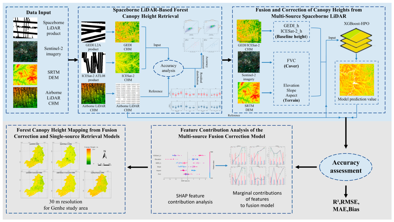
The methodological framework of this study consists of two main stages: single-source spaceborne LiDAR-based canopy height retrieval (Section 3.1), and multi-source data fusion and bias correction (Section 3.2). Figure 2 shows the flowchart of the multi-source spaceborne LiDAR data fusion and correction framework.

3.1. Spaceborne LiDAR-Based Forest Canopy Height Retrieval

Spaceborne LiDAR-derived spatially continuous canopy height maps serve as the primary input to the fusion correction model. Two main approaches are used to generate spatially continuous forest canopy height products: spatial interpolation and machine learning-based retrieval. The latter establishes statistical relationships between spaceborne LiDAR-estimated canopy heights and multi-source remote sensing features, enabling spatial extrapolation from discrete footprints to continuous canopy height products. It has become the principal method for regional-to global-scale forest canopy height mapping.
In this study, a machine learning-based approach was employed to generate spatially continuous forest canopy height products from spaceborne LiDAR footprints. After comparing the canopy height retrieval performance of multiple models, the XGBoost-HPO model was ultimately selected as the retrieval model for forest canopy height. Specifically, quality-filtered spaceborne LiDAR canopy heights were used as target variables, while Sentinel-2 spectral bands, spectral indices, and texture features served as predictors. The XGBoost model was optimized using the Tree-structured Parzen Estimator (TPE) within the Hyperopt framework, with root mean square error (RMSE) as the minimization objective under 5-fold cross-validation. A detailed description of the processing workflow is provided in Section 3.2. Finally, the quality-filtered footprints were randomly split into training and validation sets at an 8:2 ratio for model training and validation.

3.2. Fusion and Correction of Canopy Heights from Multi-Source Spaceborne LiDAR

Previous studies have shown that spaceborne LiDAR height retrievals contain systematic biases associated with terrain conditions. To address this issue, this study developed a fusion and correction model for canopy height estimates derived from multi-source spaceborne LiDAR observations. First, using airborne LiDAR canopy heights as a reference, we systematically analyzed the systematic error distributions of different spaceborne LiDAR-derived forest canopy height products under varying terrain conditions. On this basis, taking into account the differential effects of various terrain factors on canopy height products, we constructed a forest canopy height correction model based on the XGBoost algorithm. Finally, considering the discrepancies among different spaceborne LiDAR canopy height products, we developed a multi-source fusion and correction model for forest canopy height. Unlike single-source spaceborne LiDAR-based forest canopy height retrieval, the primary objective of the multi-source fusion and correction model is to correct the systematic biases in spaceborne LiDAR-derived canopy height products under different terrain conditions. Accordingly, the target variable was defined as the reference forest canopy height, which in this study was represented by the airborne LiDAR-derived canopy height (ALS_98). The predictor variables comprised the spatially continuous CHM products derived from single-source spaceborne LiDAR retrieval (GEDI-derived CHM and ICESat-2-derived CHM), together with the corresponding terrain factors (slope, aspect, and elevation) extracted from the DEM.
XGBoost is an ensemble learning algorithm based on gradient boosting decision trees (GBDT). Its objective function uses a second-order Taylor expansion to more accurately approximate the loss function, and regularization terms are included to control model complexity, thereby ensuring high predictive accuracy while effectively mitigating overfitting [41]. Compared with conventional decision tree models, XGBoost offers greater training efficiency, superior prediction accuracy, and strong interpretability. It is particularly well-suited for small-sample data, a key advantage for canopy height modeling in regions with limited plot samples. Building upon this algorithm, this study further employs the Tree-structured Parzen Estimator (TPE) within the Hyperopt framework for Bayesian hyperparameter optimization of the XGBoost model; the resulting optimized model is referred to as XGBoost-HPO. This method builds a probabilistic surrogate model from historical evaluation results to guide the search direction, approaching the global optimum with fewer evaluations than conventional grid or random search [42]. In each TPE trial, a 5-fold cross-validation was performed with the negative root mean square error (negRMSE) as the minimization objective, and each optimization run consisted of 80 evaluations. To assess the sensitivity of model performance to the stochastic nature of TPE sampling, a multi-seed screening strategy was adopted: the HPO procedure was repeated across 12 independent random seeds, each controlling the TPE initialization, while the XGBoost model random state was held fixed at 42. Prior to modeling, all features were standardized to zero mean and unit variance using the StandardScaler.
Given the relatively limited number of airborne sample plots (n = 46), a leave-one-out cross-validation (LOOCV) strategy was adopted to maximize the utility of the available data. As an extreme case of k-fold cross-validation, LOOCV iteratively uses n-1 samples for training and the single remaining sample for validation, ensuring that every plot contributes to both model training and independent assessment. This approach provides a nearly unbiased estimate of generalization error while making efficient use of the limited sample size, which is particularly critical for building reliable correction models in data-scarce regions. Accordingly, LOOCV was applied to evaluate the performance of multi-source fusion and correction model.

3.3. Accuracy Evaluation Metrics

Five metrics were selected to quantitatively evaluate the model’s performance: the coefficient of determination (R2), root mean square error (RMSE), mean absolute error (MAE), bias, and Pearson correlation coefficient (r). R2 measures the proportion of variance in the target variable explained by the model, with values closer to 1 indicating a better fit. RMSE quantifies the root-mean-squared deviation between predicted and observed values. MAE quantifies the mean absolute deviation between predicted and observed values. Bias quantifies the overall systematic deviation of the model, indicating a tendency toward overestimation (positive values) or underestimation (negative values). The Pearson correlation coefficient (r) measures the strength and direction of the linear relationship between predicted and observed values, with values closer to 1 or −1 indicating a stronger linear association. In this study, R2 was reported for internal model evaluation to assess the proportion of variance explained, while the Pearson correlation coefficient (r) was used for external comparison against independent airborne LiDAR reference data to measure linear association strength. Bias was reported alongside RMSE and MAE in all comparisons to quantify systematic deviation. The five metrics can be expressed as follows:
R 2 = 1 i = 1 n y i y ˆ i 2 i = 1 n y i y ¯ 2
R M S E = 1 n i = 1 n y i y ˆ i 2
M A E = 1 n i = 1 n y i y ˆ i
B i a s = 1 n i = 1 n y ˆ i y i
r = i = 1 n y i y ¯ y ˆ i y ˆ ¯ i = 1 n y i y ¯ 2 i = 1 n y ˆ i y ˆ ¯ 2
where n is the total number of samples, y i   is the reference measurement of the i-th sample, y ˆ i   is the model prediction of the i-th sample, y ¯   is the mean of all reference measurements, and y ˆ   ¯ is the mean of all model predictions.

3.4. Model Interpretation Using SHAP Analysis

To interpret the contribution of each predictor variable to the XGBoost-HPO models, we employed SHAP (SHapley Additive exPlanations) analysis. SHAP is a unified game-theoretic framework that assigns importance values to each feature for each individual prediction, providing both global and local interpretability. The SHAP value for a given feature quantifies its average marginal contribution to the prediction across all possible feature subsets, satisfying properties of consistency and local accuracy. We used the TreeExplainer implementation from the SHAP Python library (version 0.52.0, released May 2026), which is specifically optimized for tree-based ensemble models such as XGBoost. SHAP analysis was applied to the trained models to identify the most influential predictors and their directional effects on canopy height estimates.

4. Results and Analysis

4.1. Forest Canopy Height Retrieval from Different Spaceborne LiDAR

We constructed two separate forest canopy height retrieval models for the Genhe area using the XGBoost-HPO model with Bayesian hyperparameter optimization. The models incorporated canopy height estimates from GEDI and ICESat-2, along with remote sensing features as inputs.
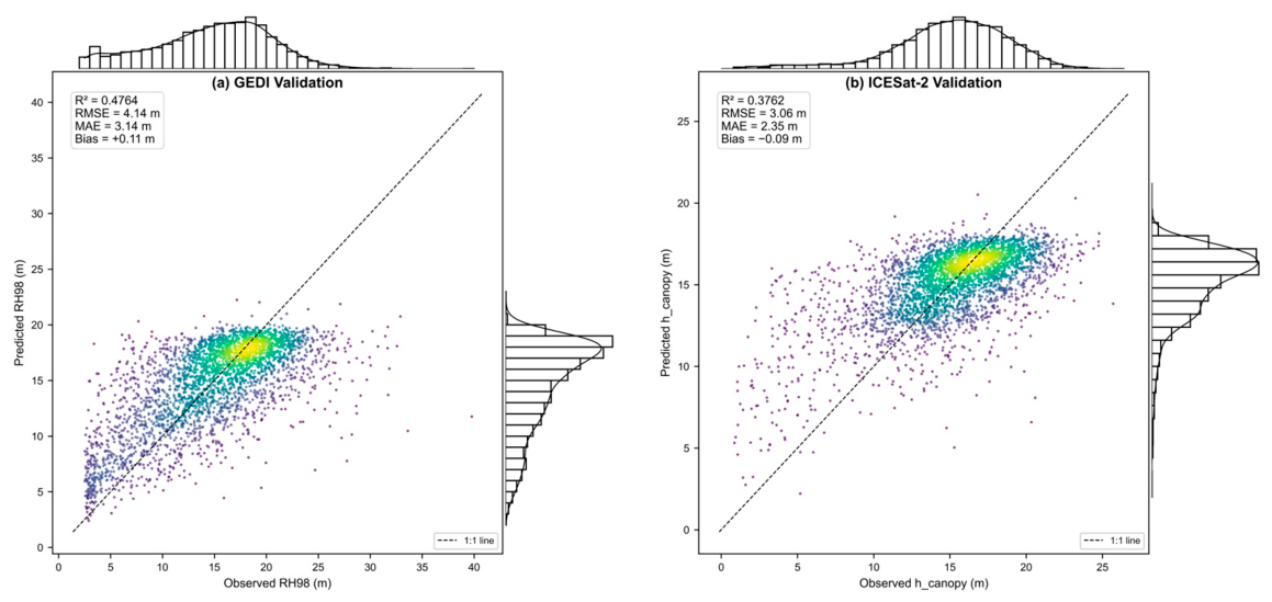
Figure 3 shows scatter plots of observed versus predicted forest canopy heights from different spaceborne LiDAR retrievals on the validation set. ICESat-2 achieved a lower RMSE (3.06 m) than GEDI (4.14 m), whereas GEDI yielded a higher R2 (0.476) than ICESat-2 (0.376). This indicates that GEDI explained a greater proportion of the target variance but had larger absolute deviations, whereas ICESat-2 showed smaller errors but less explanatory power. This discrepancy may be attributable to differences in the sample distributions between the two datasets. Specifically, GEDI validation footprints exhibited a wider height distribution (Figure 3, marginal histograms), covering a broader range of canopy height values, which provided greater explanatory scope for R2 but also increased the absolute prediction error. In contrast, ICESat-2 validation footprints showed a narrower height distribution, leading to smaller absolute errors (lower RMSE) but a correspondingly lower R2 due to limited target variance. These contrasts underscore the importance of integrating multi-source spaceborne LiDAR data to improve sample coverage and model robustness.
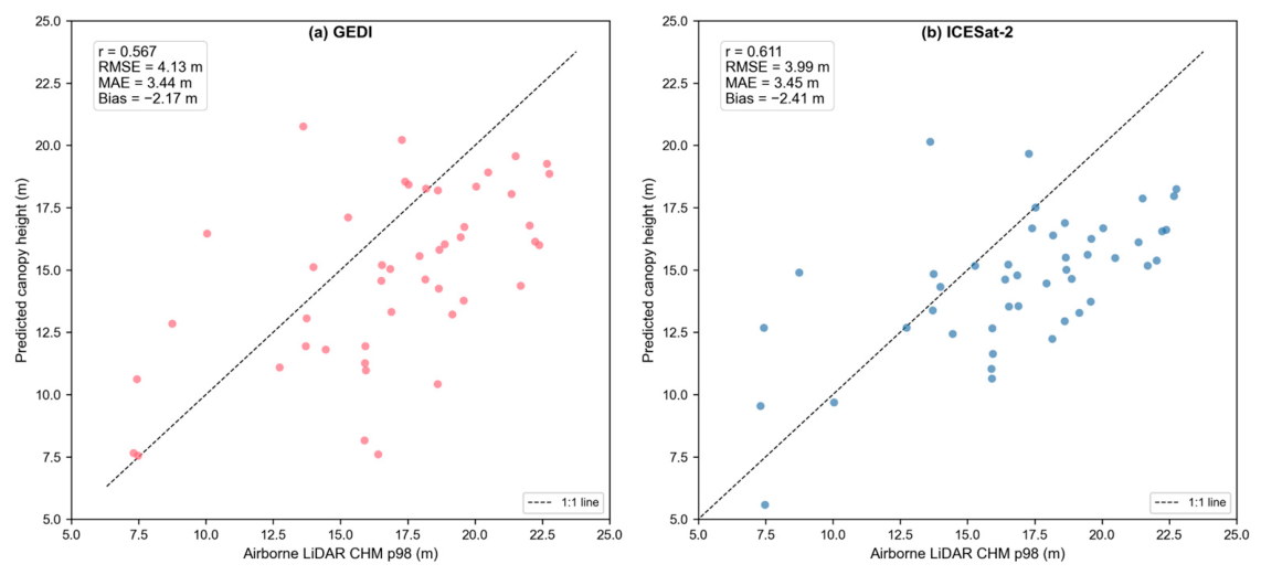
To validate the spaceborne LiDAR-retrieved canopy heights against true forest heights, we compared them with airborne LiDAR-derived canopy heights. Figure 4 shows scatter plots comparing airborne LiDAR-derived forest canopy height with spaceborne LiDAR-derived canopy height. Compared with the airborne LiDAR CHM p98 across the 46 plots, GEDI achieved RMSE = 4.13 m, MAE = 3.44 m, and bias = −2.17 m, whereas ICESat-2 achieved RMSE = 3.99 m, MAE = 3.45 m, and bias = −2.41 m. Regarding correlation, the Pearson correlation coefficient between ICESat-2-retrieved canopy heights and airborne-derived canopy heights was slightly higher (r = 0.611) than that for GEDI (r = 0.567). In addition, both retrievals were systematically underestimated by more than 2 m (GEDI: −2.17 m; ICESat-2: −2.41 m). Overall, ICESat-2 slightly outperformed GEDI in overall accuracy across the Genhe area.
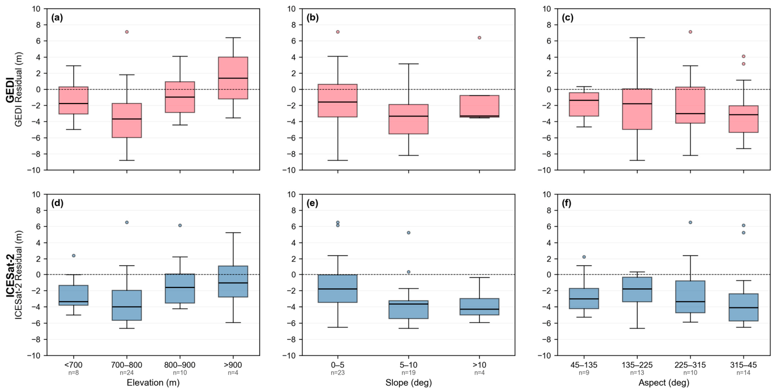
We further investigate the residual distribution patterns of spaceborne LiDAR-derived forest canopy height products across different environmental conditions, as shown in Figure 5. Overall, both the median and mean residuals for spaceborne LiDAR-retrieved forest canopy heights were mostly below zero, indicating that spaceborne LiDAR generally underestimates the actual canopy heights. Specifically, in terms of elevation, the residual trends of GEDI- and ICESat-2-based retrievals were broadly consistent, with the most severe underestimation occurring in the mid-elevation zone (700–800 m) and gradually diminishing toward both lower and higher elevations. It should be noted that, at high elevations (>900 m), the two sensors exhibited divergent responses: ICESat-2 retrievals tended to underestimate canopy heights, whereas GEDI retrievals showed slight overestimation. This complementary pattern provides an important basis for the synergistic fusion of the two datasets in high-elevation, complex forest areas. For slope, both GEDI and ICESat-2 retrievals showed systematic underestimation that increased with slope. This trend reflects an inherent challenge for spaceborne LiDAR in non-flat terrain: steeper slopes amplify topographic relief within the footprint, making it more difficult to separate ground and canopy returns and thereby introducing a systematic negative bias in canopy height estimates. Regarding the aspect, the residuals of GEDI and ICESat-2 retrievals showed systematic biases across all orientations, with bias magnitudes varying considerably among aspects. The most pronounced systematic bias occurred on north-facing slopes (315–45°), with GEDI underestimating canopy heights by 2.71 m and ICESat-2 by 2.94 m.

4.2. Fusion and Correction of Forest Canopy Height from Multi-Source Spaceborne LiDAR

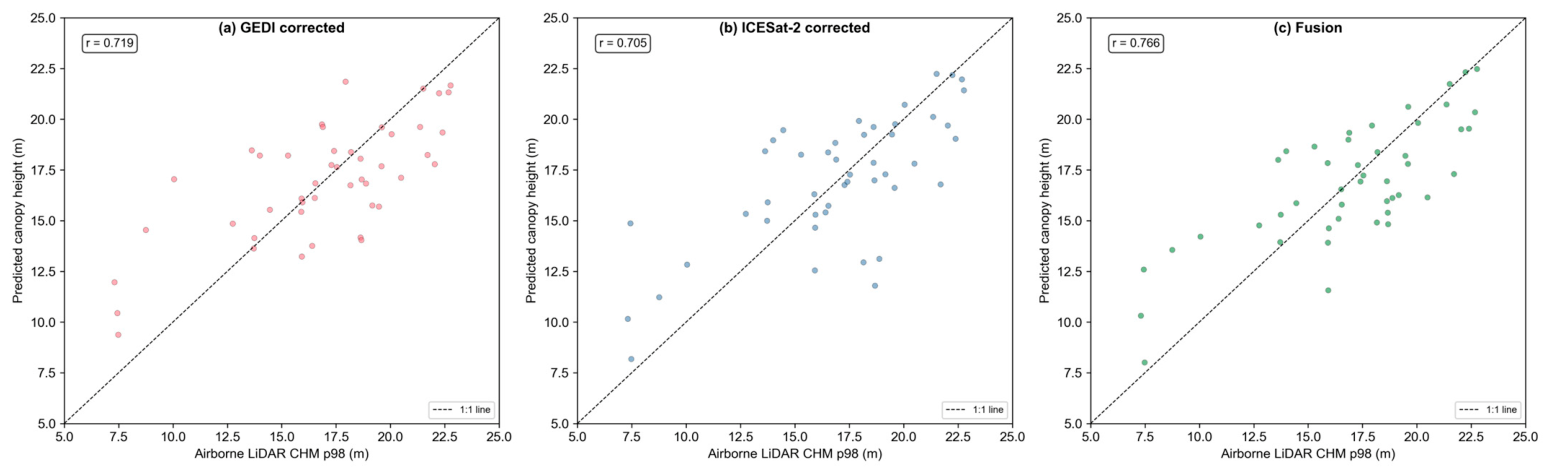
Building on the residual distribution patterns of spaceborne LiDAR-retrieved forest canopy height products across different environmental conditions, we constructed an XGBoost-based multi-source spaceborne LiDAR canopy height fusion correction model that accounts for environmental influences. Table 2 summarizes the accuracy metrics for the three retrieval results. The results show that for GEDI, the systematic bias decreased from −2.17 m to 0.00 m, effectively eliminating the underestimation; MAE decreased from 3.44 m to 2.17 m, and RMSE decreased from 4.13 m to 2.79 m, indicating a marked improvement in retrieval accuracy. For ICESat-2, the systematic bias decreased from −2.41 m to +0.02 m, while MAE decreased from 3.45 m to 2.20 m and RMSE decreased from 3.99 m to 2.87 m, demonstrating substantial gains in accuracy. Overall, accuracy metrics improved after correction, with particularly notable reductions in systematic bias. Furthermore, the multi-source fusion corrected product showed stronger agreement with true canopy heights, achieving an MAE of 2.11 m, an RMSE of 2.58 m and a Pearson correlation coefficient of 0.766. These results indicate that the fusion strategy effectively enhances the overall accuracy and reliability of canopy height retrievals.
Figure 6 shows the scatter plots of airborne LiDAR-derived canopy heights versus corrected spaceborne LiDAR-retrieved canopy heights. The results show that the Pearson correlation coefficients between the corrected and true canopy heights improved compared with those before correction. Specifically, the multi-source fusion-corrected product showed even stronger agreement with the true canopy heights, achieving a Pearson correlation coefficient of 0.766, indicating that fusing multi-source spaceborne LiDAR data can more effectively characterize actual forest canopy heights.

4.3. Contribution Analysis of Environmental Factors in the Fusion Correction Model

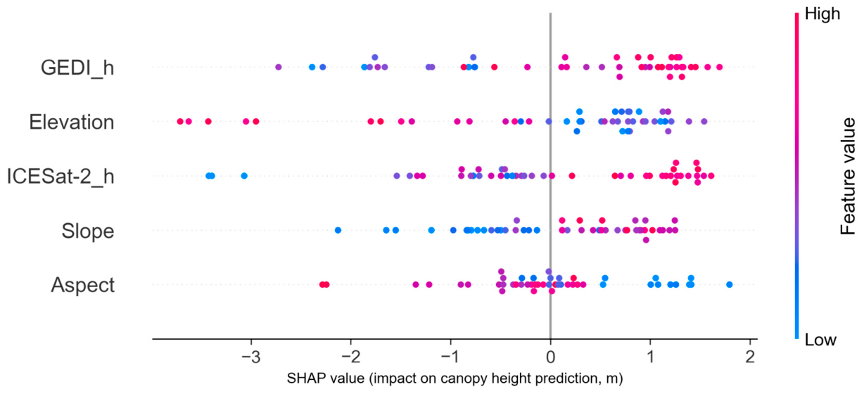
Figure 7 presents the SHAP beeswarm plot of the five predictors, ranked by mean |SHAP| value in descending order. A higher mean |SHAP| value indicates a greater overall contribution to the model prediction. Specifically, GEDI_h showed the highest mean |SHAP| value (1.14 m), followed by elevation (1.10 m) and ICESat-2_h (1.06 m). For both LiDAR-derived predictors, high feature values generally corresponded to positive SHAP values that increased the predicted canopy height, while low feature values corresponded to negative SHAP values that decreased it, indicating that GEDI_h and ICESat-2_h jointly served as the baseline canopy height reference in the fusion model, regulating the magnitude of the predictions. Elevation exhibited a clear negative gradient: high-elevation samples were associated with negative SHAP values that suppressed predictions, whereas low-elevation samples were associated with positive SHAP values that elevated predictions, consistent with the decreasing trend of canopy height with altitude in cold-temperate forests. Slope and aspect showed lower mean |SHAP| values (0.74 and 0.61 m, respectively) but still contributed to prediction adjustment as secondary terrain correction factors.
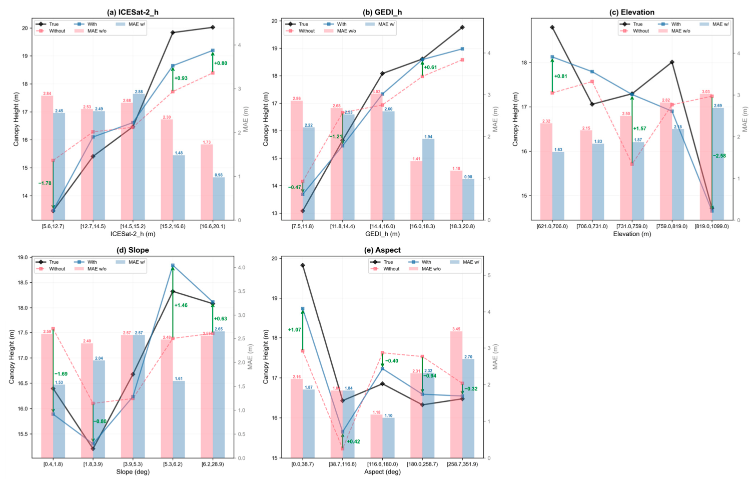
Figure 8 shows the marginal contribution of each environmental factor to forest canopy height prediction. All features had relatively pronounced marginal contributions to the model predictions; omitting them would result in obvious systematic biases. For instance, in the case of ICESat-2_h, model predictions would exhibit a systematic pattern of overestimation at low values and underestimation at high values if the canopy height reference information it carries were disregarded: at low ICESat-2_h values (<15.2 m), the SHAP values were negative, indicating that the model predictions were biased upward and required downward correction; at high ICESat-2_h values (>15.2 m), the SHAP values were positive, indicating that the model predictions were biased downward and required upward correction. This nonlinear response pattern demonstrates that ICESat-2_h exerts a bidirectional regulatory effect on the model and serves as the core feature driving the fusion correction model. GEDI_h exhibited a similar bias-correction pattern. In summary, the SHAP dependence analysis indicated that the spaceborne LiDAR retrieval products (particularly ICESat-2_h) and environmental factors such as elevation made substantial marginal contributions, and neglecting these features would lead to systematic biases. Integrating multiple spaceborne retrieval products with diverse environmental factors can more effectively correct systematic biases and enhance the prediction accuracy and robustness of the fusion correction model.
To isolate the individual contributions of environmental covariates to the correction model, we conducted a cumulative ablation experiment in which the full dual-source fusion correction model (including GEDI-derived CHM, ICESat-2-derived CHM, and three terrain factors: elevation, slope, and aspect) was used as the benchmark, and terrain factors were progressively removed to evaluate the net contribution of each covariate, with all models retaining the two LiDAR-derived CHM products as sources and using identical XGBoost-HPO configurations and LOOCV evaluation procedures. The cumulative ablation results (Table 3) demonstrate that the full model (with all five features) achieved the best performance (R2 = 0.586, RMSE = 2.58 m, Bias = −0.13 m), while progressive removal of terrain factors led to substantial performance degradation: removing aspect reduced R2 to 0.427 (ΔR2 = −0.159) and increased RMSE to 3.04 m; further removing slope decreased R2 to 0.322 (ΔR2 = −0.105) with RMSE of 3.30 m; and finally, removing elevation caused a dramatic drop to R2 = 0.166 (ΔR2 = −0.156) with RMSE of 3.66 m. These results indicate that all three terrain factors contribute significantly to the correction model, with aspect (ΔR2 = −0.159) and elevation (ΔR2 = −0.156) showing relatively larger contributions, followed by slope (ΔR2 = −0.105), and when all terrain factors were excluded, the model largely lost its correction capability (R2 = 0.166), further confirming the critical role of terrain factors in correcting systematic biases in spaceborne LiDAR canopy height products.

4.4. Forest Canopy Height Mapping

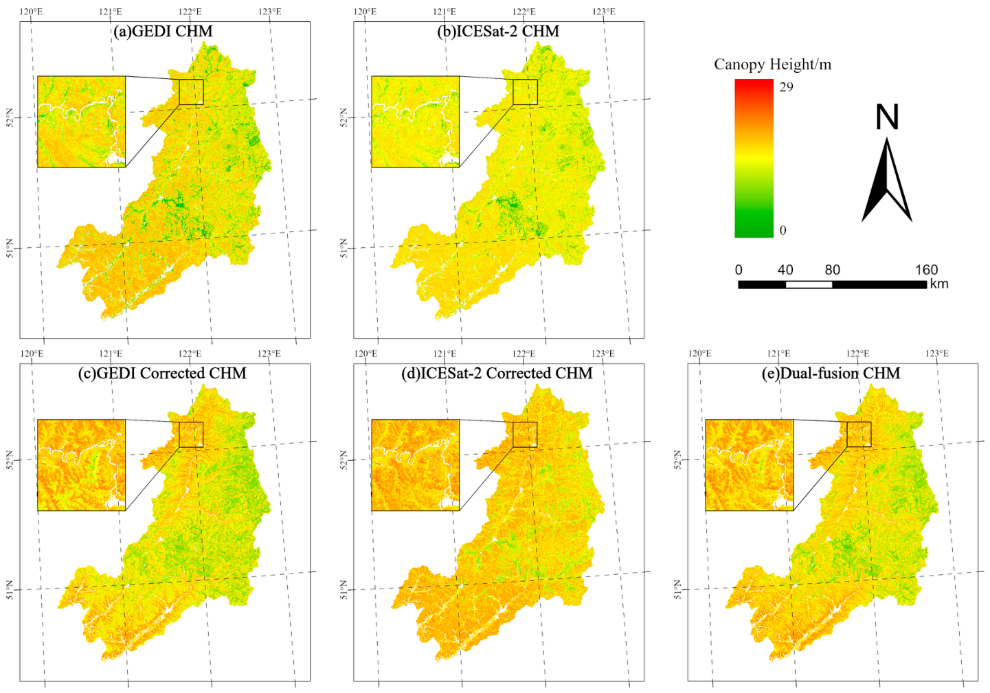
Using the constructed multi-source spaceborne LiDAR fusion correction model, we generated forest canopy height maps for the Genhe area, as shown in Figure 9. For comparison, we also produced conventional spaceborne LiDAR canopy height products and their corresponding corrected canopy height maps. Regarding spatial distribution patterns, all retrieval products effectively captured the overall east–west gradient in forest canopy height across the study area, with higher values in the west and lower values in the east. The spatial variation in canopy height was broadly consistent with the regional topographic trend. Compared with the ICESat-2-based product, the GEDI-based product exhibited more pronounced spatial variability at the regional scale. After correcting for environmental factors, the spatial distributions of the retrieval products changed markedly. For the GEDI corrected product, low- and high-value zones became more clustered, with enhanced spatial autocorrelation—consistent with Tobler’s First Law of Geography—while pronounced spatial differentiation in canopy height was preserved. For the ICESat-2 corrected product, the overall canopy height values were effectively elevated; however, the degree of spatial differentiation between high- and low-value zones was less pronounced than in the GEDI product. Furthermore, the multi-source fusion result, which synergistically integrated GEDI and ICESat-2 data, exhibited the most pronounced spatial differentiation, with sharper contrasts between high- and low-value zones and a more accurate representation of canopy height spatial heterogeneity. Overall, the multi-source spaceborne LiDAR fusion-corrected forest canopy height product showed the strongest agreement with the actual spatial distribution pattern, enabling more accurate, finer-scale characterization of the forest canopy height distribution across the Genhe study area.

5. Discussion

This study proposed a multi-source spaceborne LiDAR forest canopy height fusion and correction method based on XGBoost-HPO, and systematically validated its performance in a topographically complex region. The results demonstrate that the proposed method effectively corrects terrain-related systematic biases inherent in spaceborne LiDAR canopy height products, leading to substantial improvements in canopy height estimation accuracy. Specifically, the single-source correction models (GEDI and ICESat-2) achieved RMSE values of 2.79 m and 2.87 m under leave-one-out cross-validation, respectively, representing marked improvements over the original GEDI_h and ICESat-2_h products (RMSE = 4.13 m and 3.99 m). The dual-source fusion correction model further enhanced predictive performance, yielding an RMSE of 2.58 m under LOOCV, confirming that the integration of multi-source observations effectively complements the individual terrain sensitivities of each sensor and produces more robust canopy height estimates. These findings corroborate the effectiveness and reliability of the proposed two-stage correction strategy for regional-scale forest height mapping.
Compared with previous spaceborne LiDAR-based forest canopy height mapping studies, our fusion-corrected results demonstrate competitive accuracy. For instance, Liu et al. reported RMSE = 3.72 m for a bias-corrected ICESat-2–GEDI fusion product in Puerto Rican tropical forests [24]. Liu et al. reported RMSE = 4.88–5.32 m for a neural network-guided GEDI–ICESat-2 interpolation product over China [23]. Notably, existing fusion studies typically require either strict spatial coincidence among different spaceborne LiDAR footprints or precise matching between airborne LiDAR plots and spaceborne footprints [23,24], which are often difficult to satisfy in practice. The fusion and correction strategy of our study does not require one-to-one spatial correspondence between airborne plots and spaceborne footprints, nor does it require overlap among different spaceborne LiDAR footprints. This greatly enhances the operational feasibility of data integration and systematic error correction, making our method more adaptable and transferable for large-area applications. It should also be noted that the spatial scales of GEDI RH98 (~25 m) and ICESat-2 ATL08 h_canopy (100 m along-track segment) are inherently different. Although we resampled both products to a common 30 m grid to enable a consistent comparative framework, this upscaling inevitably simplifies the fine-scale variability captured by GEDI and may not fully account for the scale mismatch between the two sensors. Future research should explore scale-adaptive fusion approaches, such as footprint-level aggregation or multi-scale modeling, to more rigorously address this issue.
The successful acquisition of airborne LiDAR data was a critical prerequisite for implementing this study. However, due to the high cost of airborne LiDAR data and the challenging geographic and transportation conditions in the Genhe study area, only 46 field plots with airborne observations were obtained. These plots exhibited a certain degree of spatial imbalance, being predominantly concentrated in low-elevation areas, whereas high-elevation and steep-terrain zones were sparsely sampled. The limited number and uneven distribution of field plots may introduce several limitations. On the one hand, certain environmental factors (e.g., slope classes and aspect types) may be underrepresented in the training samples, leading the model to learn their effects poorly and, consequently, to underestimate or neglect their corrective roles under these specific conditions. On the other hand, the spatial bias in plot distribution may compromise the model’s generalization capability, particularly in sparsely sampled high-elevation or complex-terrain areas, where uncertainty in correction performance may be greater. This also partly explains the relatively low SHAP contributions of certain environmental factors (e.g., aspect) observed in this study. Future research should aim to increase the number of airborne LiDAR field plots and adopt a stratified random sampling strategy to ensure a balanced distribution of samples across elevation, slope and aspect. In addition, it should be noted that the terrain variables used in this study—elevation, slope, and aspect—were derived from SRTM C-band data. Since the C-band radar signal penetrates vegetation only partially, the SRTM-derived elevations in forested areas represent a mixed reflection surface between the canopy and the ground, rather than true bare earth elevations. This vegetation-induced bias in the SRTM DEM, which may vary with forest structure and density, could influence the extraction of terrain metrics and consequently affect the correction model’s performance. While the use of SRTM data was motivated by its consistent and wall-to-wall coverage across our study area, we acknowledge that the residual vegetation signal in the DEM may introduce uncertainties in the terrain-driven bias correction, particularly in densely forested and steeply sloping areas. Future studies could improve upon this limitation by utilizing high-resolution LiDAR-derived DEMs or fusion products that provide more accurate bare earth elevations, such as the ALOS World 3D or FABDEM, wherever available.
Rigorous quality screening is an essential prerequisite for spaceborne LiDAR-based forest canopy height retrieval. Following established practices, this study conducted multi-criteria quality screening of the ICESat-2 ATL08 and GEDI L2A data. Although this process effectively ensures the quality of modeling samples, it introduces two issues. First, a large number of footprints are discarded, wasting valuable observations. Second, the retained high-quality footprints are not homogeneous in accuracy; their reliability varies markedly across different environmental conditions (i.e., heteroscedasticity exists). In areas with flat terrain and simple canopy structure, estimates are generally more accurate, whereas in steep terrain with complex canopy structure, even screened footprints may still suffer from terrain shadows and canopy multiple scattering, leading to increased uncertainty. Most existing studies overlook this heteroscedasticity, treating all retained footprints as equally reliable during model training. Our current framework follows this conventional practice, which may cause the model to underfit high-accuracy regions while overfitting low-accuracy regions, compromising generalization across diverse conditions. However, the primary objective of this study is to address terrain-related systematic biases rather than random heteroscedastic uncertainty. Weighting strategies can mitigate random errors by downweighting high-uncertainty samples, but systematic biases require structural correction through model design rather than reweighting. For future work, we plan to explore sample-weighting approaches within the XGBoost framework to further enhance model robustness in complex mountainous regions.
It should be noted that the fusion and correction framework developed in this study was built upon the L2 canopy height products of GEDI L2A and ICESat-2 ATL08, rather than directly retrieving canopy height from raw waveform or photon-cloud observations. This choice was primarily motivated by operational feasibility. The L2 products are generated by the respective mission science teams through standardized processing and quality control procedures, providing consistent and reproducible canopy height metrics at regional scales that have been widely adopted in forest structure mapping studies. In contrast, direct extraction of canopy height from raw observations, such as GEDI L1B full waveforms or ICESat-2 ATL03 photon-cloud data, requires complex preprocessing steps, including waveform decomposition, photon classification, and noise filtering. Each of these steps involves parameter selection and algorithmic uncertainties, while independent reference data at the footprint scale for reliability validation remain unavailable. Consequently, direct utilization of raw data for accurate and generalizable canopy height retrieval at regional scales still faces substantial technical challenges.
Nevertheless, we acknowledge that the existing L2 products themselves contain terrain-related systematic biases, which served as the core motivation for constructing the fusion and correction model in this study. Through the two-stage design, which first establishes the spectral-to-height statistical relationship and then performs bias correction using terrain variables as predictors, we have partially compensated for the terrain sensitivity deficiencies of the existing products. However, other sources of uncertainty not fully captured by terrain factors, such as atmospheric conditions, land cover types, and seasonal variations, may still affect the accuracy of the final products. Future research could explore the following directions. First, more robust algorithms for raw data processing could be developed, leveraging deep learning approaches to directly extract canopy height from GEDI waveforms and ICESat-2 photon-cloud data, thereby reducing dependence on intermediate products. Second, multi-temporal spaceborne LiDAR observations could be integrated to reduce the uncertainty of single-shot measurements through repeated sampling. Third, additional auxiliary variables, such as climate, soil properties, and forest types, could be incorporated into the fusion framework to further explain residual heterogeneity. With the accumulation of spaceborne LiDAR data and advances in algorithms, direct generation of high-accuracy regional canopy height models from raw observations will become increasingly feasible, effectively avoiding the propagation of uncertainties inherent in current intermediate-product-dependent approaches.

6. Conclusions

In this study, we used airborne LiDAR-derived canopy heights as a reference baseline to systematically validate the effectiveness of conventional spaceborne LiDAR canopy height retrievals and to analyze the distribution patterns of retrieval residuals across different geographic environmental factors. On this basis, we further incorporated the differential effects of environmental factors to develop a multi-source spaceborne LiDAR canopy height fusion correction model. The model’s effectiveness was validated in the Genhe area, and a 30 m spatial-resolution forest canopy height map for the study area was generated. The main conclusions are as follows:
(1)
Spaceborne LiDAR provides an important data foundation for regional- and global-scale forest canopy height estimation, demonstrating its feasibility for canopy height retrieval. The retrieval results show that the GEDI and ICESat-2 models achieved R2 values of 0.476 and 0.376, with RMSE values of 4.14 m and 3.06 m, respectively, indicating that both models captured the spatial variability of canopy height to a reasonable degree. However, considerable systematic biases remained between the retrievals and true canopy heights: GEDI showed a systematic underestimation (bias = −2.17 m), and ICESat-2 exhibited a similar pattern (bias = −2.41 m). Residual distribution analysis further revealed that these systematic biases varied across different environmental conditions.
(2)
By accounting for the effects of complex environmental factors, this study substantially corrected the systematic biases inherent in spaceborne LiDAR retrievals and improved the reliability of the results. After correction, GEDI RMSE decreased from 4.13 m to 2.79 m (a 32.4% reduction), and bias shifted from −2.17 m to +0.00 m. For ICESat-2, RMSE decreased from 3.99 m to 2.87 m (a 28.1% reduction), and bias shifted from −2.41 m to +0.02 m. These findings confirm that environmental covariates effectively explain the primary sources of systematic bias in spaceborne LiDAR canopy height estimates.
(3)
Compared with single-source spaceborne LiDAR retrievals, the multi-source fusion-corrected forest canopy height product demonstrated clear advantages in both accuracy and reliability. The multi-source fusion correction model further reduced the RMSE to 2.58 m and increased the correlation coefficient r to 0.766, with a bias of −0.13 m, indicating that no additional systematic bias was introduced. The SHAP-based feature importance assessment identified ICESat-2_h and GEDI_h as the dominant features driving the correction model’s predictions, with marginal contributions substantially higher than those of the environmental covariates (slope and aspect), further confirming the irreplaceable role of spaceborne LiDAR data in forest canopy height retrieval. Spatially, the fusion product exhibited clearer boundaries in tall-canopy zones and more natural transitions between low- and high-canopy areas, demonstrating stronger spatial agreement with airborne LiDAR reference measurements.

Author Contributions

Conceptualization, S.C. and H.S.; methodology, H.Z., S.C. and H.S.; software, H.Z. and S.Q.; validation, H.Z., M.C. and S.Q.; formal analysis, H.Z. and S.C.; investigation, S.C. and H.Z.; resources, S.C.; data curation, S.Q. and M.C.; writing—original draft preparation, H.Z., S.C.; writing—review and editing, S.C., H.S., M.C. and S.Q.; visualization, H.Z.; supervision, S.C., H.S., S.Q. and M.C.; project administration, S.C., M.C.; funding acquisition, S.C. and H.S. All authors have read and agreed to the published version of the manuscript.

Funding

This research was Supported by Hunan Engineering Research Center of Natural Ecosystems Carbon Sink Monitoring (Grant No. 2025HNNCS05), the Scientific Research Project of Hunan Provincial Department of Education (Grant No. 25B0311), the 14th Five-Year National Key Research and Development Program of China (Grant No. 2023YFD2201703), the National Natural Science Foundation of China (Grant No. 32471861), and the Hunan Provincial Science and Technology Innovation Program (Science and Technology Innovation Leading Talent Project) (Grant No. 2023RC1065).

Data Availability Statement

The Sentinel-2 Level-2A surface reflectance product and the SRTM digital elevation model are available through Google Earth Engine (https://developers.google.com/earth-engine/datasets/; accessed on 17 May 2026). The GEDI L2A product can be obtained from the U.S. Geological Survey (https://lpdaac.usgs.gov/products/gedi02_av002/; accessed on 17 May 2026), and the ICESat-2 ATL08 product is available from the National Snow and Ice Data Center (https://nsidc.org/data/atl08/; accessed on 17 May 2026).

Acknowledgments

We express our sincere gratitude to those who provided support and advice for this article. During the preparation of this manuscript, the authors used DeepSeek (DeepSeek V4, 2025) for language editing and text refinement. The authors have reviewed and edited the output and take full responsibility for the content of this publication.

Conflicts of Interest

The authors declare no conflicts of interest.

References

  1. Pan, Y.; Birdsey, R.A.; Fang, J.; Houghton, R.; Kauppi, P.E.; Kurz, W.A.; Phillips, O.L.; Shvidenko, A.; Lewis, S.L.; Canadell, J.G.; et al. A large and persistent carbon sink in the world’s forests. Science 2011, 333, 988–993. [Google Scholar] [CrossRef] [Scilit] [PubMed]
  2. Coops, N.C.; Tompalski, P.; Goodbody, T.R.H.; Queinnec, M.; Luther, J.E.; Bolton, D.K.; White, J.C.; Wulder, M.A.; van Lier, O.R.; Hermosilla, T. Modelling lidar-derived estimates of forest attributes over space and time: A review of approaches and future trends. Remote Sens. Environ. 2021, 260, 112477. [Google Scholar] [CrossRef] [Scilit]
  3. Lang, N.; Jetz, W.; Schindler, K.; Wegner, J.D. A high-resolution canopy height model of the Earth. Nat. Ecol. Evol. 2023, 7, 1778–1789. [Google Scholar] [CrossRef] [Scilit] [PubMed]
  4. De Petris, S.; Sarvia, F.; Borgogno-Mondino, E. About tree height measurement: Theoretical and practical issues for uncertainty quantification and mapping. Forests 2022, 13, 969. [Google Scholar] [CrossRef] [Scilit]
  5. Dubayah, R.; Blair, J.B.; Goetz, S.; Fatoyinbo, L.; Hansen, M.; Healey, S.; Hofton, M.; Hurtt, G.; Kellner, J.; Luthcke, S.; et al. The Global Ecosystem Dynamics Investigation: High-resolution laser ranging of the Earth’s forests and topography. Sci. Remote Sens. 2020, 1, 100002. [Google Scholar] [CrossRef] [Scilit]
  6. Ahmed, O.S.; Franklin, S.E.; Wulder, M.A.; White, J.C. Characterizing stand-level forest canopy cover and height using Landsat time series, samples of airborne LiDAR, and the random forest algorithm. ISPRS J. Photogramm. Remote Sens. 2015, 101, 89–101. [Google Scholar] [CrossRef] [Scilit]
  7. Liu, Y.; Gong, W.; Xing, Y.; Hu, X.; Gong, J. Estimation of the forest stand mean height and aboveground biomass in Northeast China using SAR Sentinel-1B, multispectral Sentinel-2A, and DEM imagery. ISPRS J. Photogramm. Remote Sens. 2019, 151, 277–289. [Google Scholar] [CrossRef] [Scilit]
  8. Wolter, P.T.; Townsend, P.A.; Sturtevant, B.R. Estimation of forest structural parameters using 5 and 10 meter SPOT-5 satellite data. Remote Sens. Environ. 2009, 113, 2019–2036. [Google Scholar] [CrossRef] [Scilit]
  9. Zarco-Tejada, P.J.; Diaz-Varela, R.; Angileri, V.; Loudjani, P. Tree height quantification using very high resolution imagery acquired from an unmanned aerial vehicle (UAV) and automatic 3D photo-reconstruction methods. Eur. J. Agron. 2014, 55, 89–99. [Google Scholar] [CrossRef] [Scilit]
  10. Dube, T.; Mutanga, O. Investigating the robustness of the new Landsat-8 Operational Land Imager derived texture metrics in estimating plantation forest aboveground biomass in resource constrained areas. ISPRS J. Photogramm. Remote Sens. 2015, 108, 12–32. [Google Scholar] [CrossRef] [Scilit]
  11. Joshi, N.; Mitchard, E.T.A.; Brolly, M.; Schumacher, J.; Fernández-Landa, A.; Johannsen, V.K.; Marchamalo, M.; Fensholt, R. Understanding ‘saturation’ of radar signals over forests. Sci. Rep. 2017, 7, 3505. [Google Scholar] [CrossRef] [Scilit] [PubMed]
  12. Lim, K.; Treitz, P.; Wulder, M.; St-Onge, B.; Flood, M. LiDAR remote sensing of forest structure. Prog. Phys. Geogr. 2003, 27, 88–106. [Google Scholar] [CrossRef] [Scilit]
  13. Brolly, G.; Király, G.; Lehtomäki, M.; Liang, X. Voxel-based automatic tree detection and parameter retrieval from terrestrial laser scans for plot-wise forest inventory. Remote Sens. 2021, 13, 542. [Google Scholar] [CrossRef] [Scilit]
  14. Andersen, H.-E.; Reutebuch, S.E.; McGaughey, R.J. A rigorous assessment of tree height measurements obtained using airborne lidar and conventional field methods. Can. J. Remote Sens. 2006, 32, 355–366. [Google Scholar] [CrossRef] [Scilit]
  15. Chen, Y.; Yang, H.; Yang, Z.; Yang, Q.; Liu, W.; Huang, G.; Ren, Y.; Cheng, K.; Xiang, T.; Chen, M.; et al. Enhancing high-resolution forest stand mean height mapping in China through an individual tree-based approach with close-range lidar data. Earth Syst. Sci. Data 2024, 16, 5267–5285. [Google Scholar] [CrossRef] [Scilit]
  16. Markus, T.; Neumann, T.; Martino, A.; Abdalati, W.; Brunt, K.; Csatho, B.; Farrell, S.; Fricker, H.; Gardner, A.; Harding, D.; et al. The Ice, Cloud, and land Elevation Satellite-2 (ICESat-2): Science requirements, concept, and implementation. Remote Sens. Environ. 2017, 190, 260–273. [Google Scholar] [CrossRef] [Scilit]
  17. Potapov, P.; Li, X.; Hernandez-Serna, A.; Tyukavina, A.; Hansen, M.C.; Kommareddy, A.; Pickens, A.; Turubanova, S.; Tang, H.; Silva, C.E.; et al. Mapping global forest canopy height through integration of GEDI and Landsat data. Remote Sens. Environ. 2021, 253, 112165. [Google Scholar] [CrossRef] [Scilit]
  18. Tiwari, K.; Narine, L.L. A comparison of machine learning and geostatistical approaches for mapping forest canopy height over the southeastern US using ICESat-2. Remote Sens. 2022, 14, 5651. [Google Scholar] [CrossRef] [Scilit]
  19. Liu, A.; Cheng, X.; Chen, Z. Performance evaluation of GEDI and ICESat-2 laser altimeter data for terrain and canopy height retrievals. Remote Sens. Environ. 2021, 264, 112571. [Google Scholar] [CrossRef] [Scilit]
  20. Sothe, C.; Gonsamo, A.; Lourenço, R.B.; Kurz, W.A.; Snider, J. Spatially continuous mapping of forest canopy height in Canada by combining GEDI and ICESat-2 with PALSAR and Sentinel. Remote Sens. 2022, 14, 5158. [Google Scholar] [CrossRef] [Scilit]
  21. Zhu, X.; Nie, S.; Wang, C.; Xi, X.; Lao, J.; Li, G. Consistency analysis of forest height retrievals between GEDI and ICESat-2. Remote Sens. Environ. 2022, 281, 113244. [Google Scholar] [CrossRef] [Scilit]
  22. Liang, H.; Bie, Q.; Shi, Y.; Deng, X.; Li, X. Estimation of canopy height by integrating multi-source remote sensing data from ICESat-2 and GEDI. Remote Sens. Technol. Appl. 2025, 40, 202–214. (In Chinese) [Google Scholar]
  23. Liu, X.; Su, Y.; Hu, T.; Yang, Q.; Liu, B.; Deng, Y.; Tang, H.; Tang, Z.; Fang, J.; Guo, Q. Neural network guided interpolation for mapping canopy height of China’s forests by integrating GEDI and ICESat-2 data. Remote Sens. Environ. 2022, 269, 112844. [Google Scholar] [CrossRef] [Scilit]
  24. Liu, A.; Chen, Y.; Cheng, X. Improving tropical forest canopy height mapping by fusion of Sentinel-1/2 and bias-corrected ICESat-2–GEDI data. Remote Sens. 2025, 17, 1968. [Google Scholar] [CrossRef] [Scilit]
  25. Bai, X.; Sadia, S.; Yu, J. The variation of species diversity, regeneration and community structure in Larix gmelinii forest shaping by local environment factors. Russ. J. Ecol. 2021, 52, 275–282. [Google Scholar] [CrossRef] [Scilit]
  26. Wei, X.; Yue, F.; Deng, R.; Yan, Z.; Tong, B.; Yang, X.; Li, D. Community characteristics and species diversity of cold-temperate coniferous forests in the Daxing’anling Mountains. For. Eng. 2025, 41, 657–665. (In Chinese) [Google Scholar] [CrossRef]
  27. Xu, H. Forests of the Daxing’anling Mountains in China; Science Press: Beijing, China, 1998. (In Chinese) [Google Scholar]
  28. Neuenschwander, A.; Pitts, K. The ATL08 land and vegetation product for the ICESat-2 mission. Remote Sens. Environ. 2019, 221, 247–259. [Google Scholar] [CrossRef] [Scilit]
  29. Neuenschwander, A.; Guenther, E.; White, J.C.; Duncanson, L.; Montesano, P. Validation of ICESat-2 terrain and canopy heights in boreal forests. Remote Sens. Environ. 2020, 251, 112110. [Google Scholar] [CrossRef] [Scilit]
  30. Sang, M.; Xiao, H.; Jin, Z.; He, J.; Wang, N.; Wang, W. Improved mapping of regional forest heights by combining denoise and LightGBM method. Remote Sens. 2023, 15, 5436. [Google Scholar] [CrossRef] [Scilit]
  31. Drusch, M.; Del Bello, U.; Carlier, S.; Colin, O.; Fernandez, V.; Gascon, F.; Hoersch, B.; Isola, C.; Laberinti, P.; Martimort, P.; et al. Sentinel-2: ESA’s optical high-resolution mission for GMES operational services. Remote Sens. Environ. 2012, 120, 25–36. [Google Scholar] [CrossRef] [Scilit]
  32. Gorelick, N.; Hancher, M.; Dixon, M.; Ilyushchenko, S.; Thau, D.; Moore, R. Google Earth Engine: Planetary-scale geospatial analysis for everyone. Remote Sens. Environ. 2017, 202, 18–27. [Google Scholar] [CrossRef] [Scilit]
  33. Haralick, R.M.; Shanmugam, K.; Dinstein, I. Textural features for image classification. IEEE Trans. Syst. Man Cybern. 1973, SMC-3, 610–621. [Google Scholar] [CrossRef] [Scilit]
  34. Rouse, J.W.; Haas, R.H.; Schell, J.A.; Deering, D.W. Monitoring vegetation systems in the Great Plains with ERTS. In Proceedings of the Third Earth Resources Technology Satellite-1 Symposium; NASA SP-351; NASA: Washington, DC, USA, 1974; pp. 309–317. [Google Scholar]
  35. Delegido, J.; Verrelst, J.; Alonso, L.; Moreno, J. Evaluation of Sentinel-2 red-edge bands for empirical estimation of green LAI and chlorophyll content. Sensors 2011, 11, 7063–7081. [Google Scholar] [CrossRef] [Scilit] [PubMed]
  36. Gitelson, A.A.; Keydan, G.P.; Merzlyak, M.N. Three-band model for noninvasive estimation of chlorophyll, carotenoids, and anthocyanin contents in higher plant leaves. Geophys. Res. Lett. 2006, 33, L11402. [Google Scholar] [CrossRef] [Scilit]
  37. Dash, J.; Curran, P.J. The MERIS terrestrial chlorophyll index. Int. J. Remote Sens. 2004, 25, 5403–5413. [Google Scholar] [CrossRef] [Scilit]
  38. Huete, A.R. A soil-adjusted vegetation index (SAVI). Remote Sens. Environ. 1988, 25, 295–309. [Google Scholar] [CrossRef] [Scilit]
  39. Huete, A.R.; Didan, K.; Miura, T.; Rodriguez, E.P.; Gao, X.; Ferreira, L.G. Overview of the radiometric and biophysical performance of the MODIS vegetation indices. Remote Sens. Environ. 2002, 83, 195–213. [Google Scholar] [CrossRef] [Scilit]
  40. Richardson, A.J.; Wiegand, C.L. Distinguishing vegetation from soil background information. Photogramm. Eng. Remote Sens. 1977, 43, 1541–1552. [Google Scholar]
  41. Chen, T.; Guestrin, C. XGBoost: A scalable tree boosting system. In Proceedings of the 22nd ACM SIGKDD International Conference on Knowledge Discovery and Data Mining, San Francisco, CA, USA, 13–17 August 2016; pp. 785–794. [Google Scholar] [CrossRef] [Scilit]
  42. Bergstra, J.; Bardenet, R.; Bengio, Y.; Kégl, B. Algorithms for hyper-parameter optimization. In Proceedings of the 25th Annual Conference on Neural Information Processing Systems (NIPS 2011), Granada, Spain, 12–15 December 2011; pp. 2546–2554. [Google Scholar]
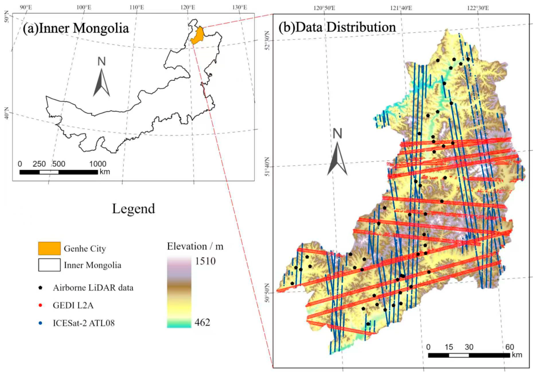
Figure 1. Geographic location of the study area.
Remotesensing 18 02787 g001
Figure 2. Flowchart of the multi-source spaceborne LiDAR data fusion and correction framework.
Remotesensing 18 02787 g002
Figure 3. Scatter plots of observed versus predicted forest canopy heights from different spaceborne LiDAR retrievals on the validation set.
Remotesensing 18 02787 g003
Figure 4. Scatter plots between airborne LiDAR-derived forest canopy height and spaceborne LiDAR-derived canopy height.
Remotesensing 18 02787 g004
Figure 5. The residual distribution patterns of spaceborne LiDAR-retrieved forest canopy height products under different environmental conditions. (a) Elevation (GEDI); (b) Slope (GEDI); (c) Aspect (GEDI); (d) Elevation (ICESat-2); (e) Slope (ICESat-2); (f) Aspect (ICESat-2).
Remotesensing 18 02787 g005
Figure 6. Scatter plots of airborne LiDAR-derived canopy heights versus corrected spaceborne LiDAR-retrieved canopy heights.
Remotesensing 18 02787 g006
Figure 7. The contributions of five environmental factors to forest canopy height prediction.
Remotesensing 18 02787 g007
Figure 8. Marginal contribution of each feature to the fusion correction model predictions.
Remotesensing 18 02787 g008
Figure 9. Forest canopy height mapping of the Genhe area from different spaceborne LiDAR before and after correction. (a) GEDI-based forest canopy height retrieval (before correction); (b) ICESat-2-based forest canopy height retrieval (before correction); (c) GEDI-based forest canopy height retrieval (after correction); (d) ICESat-2-based forest canopy height retrieval (after correction); (e) multi-source spaceborne LiDAR-based forest canopy height retrieval.
Remotesensing 18 02787 g009
Table 1. Predictive variables derived from Sentinel-2 imagery.
Feature TypeParameterDescriptionFormulaReference
Spectral
indices
NDVIReflects vegetation greenness and density(B8 − B4)/(B8 + B4)[34]
NDIReflects canopy structural density(B5 − B4)/(B5 + B4)[35]
CIREIndicates canopy chlorophyll concentration(B7/B5) − 1[36]
SRRECaptures vegetation red-edge reflectance(B7/B5)[36]
MTCIResponds to canopy chlorophyll content(B6 − B5)/(B5 − B4)[37]
SAVISuppresses soil background brightness ( B 8     B 4 )   × (1 + L)/(B8 + B4 + L),
L = 0.5
[38]
EVIReduces atmospheric and soil interference 2.5   ×   ( B 8     B 4 ) / ( B 8   +   6   ×   B 4     7.5   × B2 + 1)[39]
LAIEstimates foliage density per unit area 6.753   × (B5 − B4)/(B5 + B4)[35]
PVIMinimizes soil background interference ( B 8 B 4 ) / 2 [40]
Texture
features
EntropyMeasures canopy textural complexity i = 1 k j = 1 k P i , j log P i , j [33]
CorrelationQuantifies local textural uniformity i j i j P i , j μ x μ y σ x σ y [33]
VarianceIndicates canopy surface roughness i j i μ 2 P i , j [33]
DissimilarityCaptures fine-scale canopy height variability i = 1 k j = 1 k i j P i , j [22]
ContrastReflects local gray-level variation n = 0 N g 1 n 2 i = 1 N g   j = 1   i j = n N g P i , j [33]
Table 2. Accuracy comparison of canopy height retrieval methods.
Retrieval MethodRMSE/mMAE/mBias/mr
GEDI single-source4.133.44−2.170.567
ICESat-2 single-source3.993.45−2.410.611
GEDI corrected2.792.170.000.719
ICESat-2 corrected2.872.20+0.020.705
Dual-source fusion2.582.11−0.130.766
Table 3. Cumulative ablation experiment of the fusion correction model.
StepModelR2RMSE (m)MAE (m)Bias (m)ΔR2
0Full
(5 features)
0.5862.582.11−0.13-
1-Aspect
(4 features)
0.4273.042.36−0.02−0.159
2-Slope
(3 features)
0.3223.302.65−0.06−0.105
3-Elevation
(2 features)
0.1663.662.96−0.34−0.156
Disclaimer/Publisher’s Note: The statements, opinions and data contained in all publications are solely those of the individual author(s) and contributor(s) and not of MDPI and/or the editor(s). MDPI and/or the editor(s) disclaim responsibility for any injury to people or property resulting from any ideas, methods, instructions or products referred to in the content.