Extracting Value from Fused Aerial and Terrestrial LiDAR Scans

Highlights

This study demonstrates:

• Calibration of ULS-derived diameter at breast height (DBH) estimates using small areas of fused or terrestrial LiDAR enabled the best-performing calibration methods to reduce stand-level mean DBH differences from up to 10.4 cm to less than 1 cm.
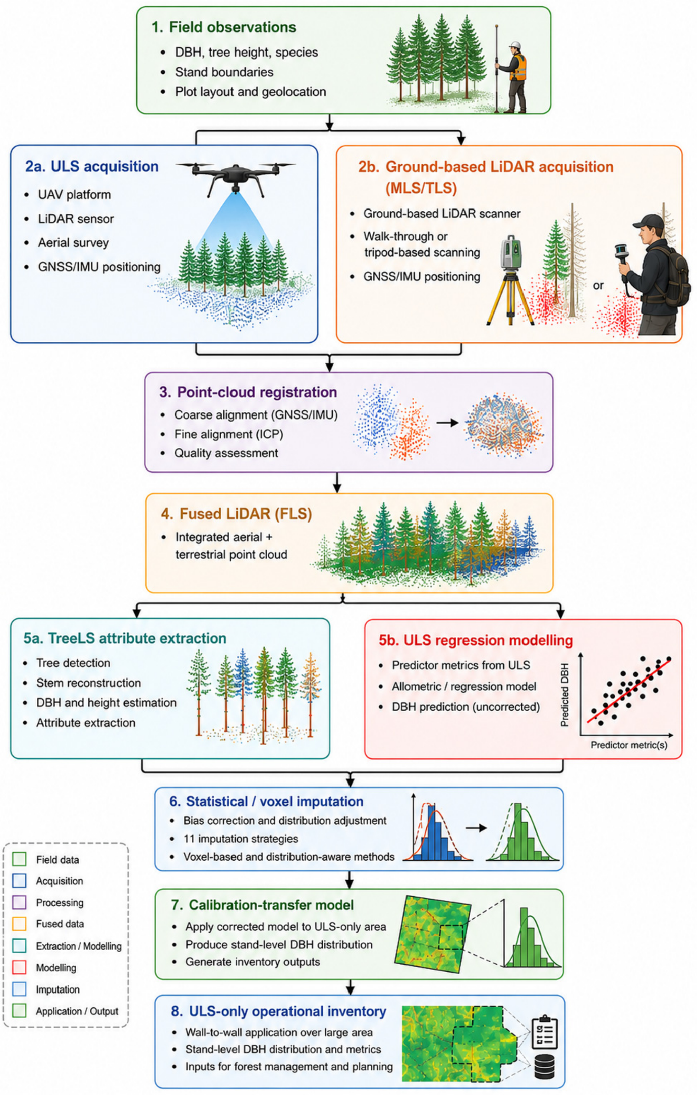
• Fusion of unmanned aerial vehicle (UAV)-based laser scanning (ULS) with mobile/terrestrial laser scanning (MLS/TLS) improved canopy completeness, structural representation, and spatial integration, providing a richer basis for stand-level inventory.
• Voxel-based imputation performed particularly well for radiata pine, while several distribution-aware calibration methods achieved comparable or better performance for mature eucalyptus.

The implications of these findings are:

• Relatively small ground-based LiDAR calibration areas showed potential to improve stand-level ULS inventory estimates across much larger surrounding survey regions.
• The combination of LiDAR fusion and distribution-aware imputation provides a practical pathway for scalable forest inventory, supporting timber assessment, carbon accounting, forest monitoring, and digital forest twin development.

Abstract

Accurate estimation of forest structural attributes over operational scales remains challenging because unmanned laser scanning (ULS) provides extensive spatial coverage but limited representation of internal stem structure, whereas terrestrial and mobile laser scanning (TLS/MLS) provide detailed stem measurements over relatively small areas. This study investigates a calibration-transfer framework in which small areas of terrestrial or fused LiDAR are used to improve diameter at breast height (DBH) estimation across much larger regions surveyed only by ULS. ULS, TLS, MLS and fused laser scanning (FLS) datasets were analysed for radiata pine and eucalyptus plantations. TreeLS-derived DBH measurements from terrestrial and fused point clouds were used as reference data to evaluate several distribution-aware and voxel-based imputation approaches for correcting regression-derived ULS estimates. Across the study sites, the best-performing imputation methods reduced stand-level mean DBH differences by as much as 95% relative to the uncorrected ULS regression estimates, resulting in substantially improved agreement with field-observed stand means while simultaneously producing DBH distributions that more closely matched the corresponding TreeLS-derived reference distributions. Voxel-based imputation performed particularly well for radiata pine and remained competitive for eucalyptus, while several distribution-based approaches achieved comparable or better performance in particular stands. These findings demonstrate the potential for transferring information from relatively small terrestrial LiDAR calibration areas to larger ULS-only acquisitions, improving stand-level DBH distribution estimates without requiring complete terrestrial coverage. Because validation was performed using stand-level field summary statistics rather than matched individual trees, the reported performance should be interpreted as demonstrating the potential of the approach under the conditions evaluated rather than universal individual-tree accuracy.

1. Introduction

Forest inventory underpins sustainable forest management, timber valuation, carbon accounting, biodiversity monitoring, and ecological research by providing quantitative information describing the structure and condition of individual trees and forest stands. Structural attributes such as diameter at breast height (DBH), total tree height (HT), crown dimensions, biomass, and stand density are fundamental inputs to growth modelling, yield prediction, and ecosystem assessment. However, conventional field inventories remain labour-intensive, expensive, spatially limited, and often constrained by accessibility, observer bias, and the structural complexity of forest environments. Consequently, there is increasing demand for remote sensing methods capable of providing accurate, repeatable, and operationally scalable forest measurements across large spatial extents [1,2,3,4,5,6,7,8,9,10,11,12,13,14].

Among available remote sensing technologies, light detection and ranging (LiDAR) has become one of the most powerful tools for three-dimensional (3D) forest characterisation because it directly measures vegetation structure rather than relying solely on spectral information. LiDAR-derived point clouds have been used extensively to estimate tree- and stand-level attributes, monitor forest dynamics, quantify biomass and carbon stocks, and support applications ranging from ecological modelling to precision forestry and digital forest twins [15,16,17,18,19,20]. Nevertheless, no single LiDAR platform simultaneously provides both detailed stem geometry and efficient landscape-scale coverage.

Ground-based terrestrial laser scanning (TLS) and mobile laser scanning (MLS) provide dense observations of stems and lower-canopy structure, enabling accurate reconstruction of individual trees and reliable extraction of structural attributes such as DBH. In contrast, unmanned laser scanning (ULS) acquired from unmanned aerial vehicles offers rapid acquisition and extensive spatial coverage but typically provides comparatively sparse observations of stems because of canopy occlusion and its predominantly overhead viewing geometry. Consequently, ULS generally performs well for canopy-level measurements but remains less reliable for direct estimation of stem attributes in dense or structurally complex forests [21].

Fusion of aerial and terrestrial LiDAR datasets provides a logical means of exploiting the complementary strengths of these platforms by combining the broad spatial coverage of ULS with the detailed structural observations obtained from ground-based LiDAR. Previous studies have shown that fused point clouds improve structural completeness, point cloud registration, stem detection, and tree attribute extraction. However, most fusion studies have focused on improving the quality of the fused point cloud itself or enhancing local structural reconstruction, rather than using the fused observations as calibration data for statistically improving inventory estimates across much larger areas surveyed only by ULS. This distinction is important because complete terrestrial coverage is rarely commercially feasible over commercial plantation estates.

Accordingly, an important research gap remains between highly accurate structural information available from relatively small terrestrial LiDAR acquisitions and the need to generate reliable inventory estimates over estate-wide spatial scales. Bridging this gap requires methods capable of transferring information from small, high-quality calibration areas to much larger aerial-only datasets while preserving realistic stand-level structural variability.

Despite these advances, significant challenges remain. ULS point clouds frequently lack sufficient stem density for reliable DBH reconstruction in dense forests, while MLS acquisitions remain operationally expensive over large areas. Moreover, the structural complexity of forests, species-specific stem morphology, canopy occlusion, and variability in laser acquisition parameters continue to limit the generalisability of many existing inventory approaches.

TLS typically refers to statically mounted ground-based instruments that are particularly effective at capturing the fine-scale details of individual trees. Their mobile (terrestrial/handheld) counterparts are usually referred to as MLS. MLS are much less time-consuming to operate and still provide clear, accurate, rapid, and high-resolution information about the complex internal features of tree structure beneath the canopy. This includes tree shape, size, branching patterns, and foliage density [21]. In this paper, MLS refers to the GeoSLAM Zeb Horizon used at Mount Crawford and TLS refers to the Leica MS50 at Cradoc. Ground-based LiDAR is used when referring to MLS and TLS collectively.

This study investigates whether a relatively small additional field effort can support calibration-transfer from ground-based to aerial LiDAR. Specifically, the study examines whether TreeLS-derived attributes from ground-based LiDAR calibration regions could be transferred reliably to nearby ULS-only areas within the same stands. The approach aims to preserve the structural accuracy of terrestrial LiDAR while leveraging the spatial scalability of aerial LiDAR, thereby showing potential to support plantation-scale forest inventory estimation.

At Mount Crawford, the handheld MLS data used to establish the calibration region was collected in approximately 15 min, illustrating the limited additional acquisition time that may be required under accessible plantation conditions. The time required in other forests will nevertheless depend on plot size, terrain, understorey density, accessibility, and the number of traverses needed to obtain representative structural coverage.

The study’s approach was as follows: (i) ULS and ground-based LiDAR point clouds are combined into a single fused laser scanning (FLS) dataset; (ii) accurate total tree height estimates are derived from the FLS; (iii) accurate stem attribute extraction tools are applied to the FLS; (iv) regression model attributes are extracted from the ULS component of the FLS; (v) the regression model estimates of the stem attributes are adjusted to match the accurate FLS estimates; and (vi) the corrected attribute model developed in the previous step is applied to the much larger section of forest observed only by the ULS.

Related Work and Research Gap

MLS and TLS have become well-established technologies for detailed forest structural characterisation because they provide dense observations of stems and lower-canopy structure. Numerous studies have demonstrated that terrestrial LiDAR enables accurate estimation of tree position, DBH, stem form, and branching architecture, making these systems valuable for forest inventory and ecological research [18,22,23,24,25,26,27,28,29,30,31,32]. However, despite their structural accuracy, terrestrial systems remain relatively time-consuming to deploy over large-scale areas and frequently experience reduced Global Navigation Satellite System (GNSS) accuracy beneath dense forest canopies, limiting the absolute positional accuracy of derived point clouds and tree locations [33,34,35,36].

ULS, in contrast, provides rapid acquisition over large areas while maintaining accurate georeferencing through unobstructed satellite visibility and differential GNSS positioning. ULS has therefore become increasingly important for production-scale forest inventory, canopy mapping, terrain modelling, biomass estimation, and monitoring forest condition [37,38,39,40,41,42,43]. Nevertheless, because aerial LiDAR primarily samples the upper canopy, point density within lower canopy and stem regions is often insufficient for reliable reconstruction of detailed stem geometry. Canopy occlusion, stand density, acquisition geometry, and sensor configuration further reduce the accuracy of direct DBH estimation in structurally complex forests, particularly in dense plantation environments [44,45,46,47,48,49,50,51].

To overcome these complementary limitations, increasing attention has been directed towards multi-platform LiDAR fusion, in which aerial and terrestrial point clouds are combined to improve structural completeness and attribute estimation [8,52,53,54,55]. FLS datasets provide observations of forest structure from both above and beneath the canopy, improving point cloud registration, stem detection, canopy representation, and structural reconstruction. Such datasets are increasingly recognised as enabling technologies for digital forest twins and multi-scale forest modelling, where detailed local observations are integrated with extensive aerial coverage to characterise forest structure across plantation landscapes. However, most previous fusion studies have focused on improving the quality of the fused point cloud itself rather than exploiting fused observations as calibration data for inventory estimation across larger aerial-only regions.

Parallel advances in machine learning, voxel-based analysis, and point cloud-driven modelling have expanded opportunities for estimating forest attributes from structurally sparse LiDAR observations [56,57,58,59]. Early approaches relied primarily on allometric or regression-based relationships linking DBH to tree height and crown dimensions [60,61,62,63,64,65], whereas more recent methods employ point cloud segmentation, stem reconstruction, voxel metrics, nearest-neighbour learning, and statistical correction techniques to improve structural attribute estimation [13,14,66,67,68]. At the stand scale, LiDAR has also been widely used to estimate canopy cover, gap fraction, leaf area index, biomass, and spatial forest structure [40,69,70,71], demonstrating the versatility of point cloud-based forest characterisation.

Imputation methods provide an attractive framework for transferring information between dense and sparse observation domains because they infer missing attributes from structurally similar observations rather than requiring complete direct measurement [72,73,74,75,76,77,78,79,80,81,82,83]. Recent developments in voxel-based modelling, empirical quantile mapping, bias-corrected conditional rank–quantile blending, and conditional residual restoration have further improved the ability of imputation methods to preserve realistic stand-level variability while correcting systematic bias. These approaches are particularly attractive for practical forest inventory because they permit accurate structural information derived from relatively small terrestrial or fused calibration areas to be transferred to much larger regions surveyed only by ULS, thereby substantially reducing field effort without requiring complete terrestrial coverage.

Despite these advances, an important gap remains. Existing studies generally seek either to improve direct attribute extraction from ULS point clouds or to enhance the quality of fused point clouds through improved registration and structural reconstruction. Comparatively little attention has been given to using small areas of high-density terrestrial or fused LiDAR as calibration regions from which statistically robust corrections can be transferred to substantially larger ULS-only acquisitions. Addressing this gap has the potential to combine the structural fidelity of terrestrial LiDAR with the scalability of aerial LiDAR, providing a practical pathway towards improved stand-level inventory estimation over operationally relevant spatial extents.

Rather than viewing terrestrial and aerial LiDAR as competing technologies, this study investigates whether they can be integrated within a calibration-transfer framework, whereby detailed structural information extracted from relatively small areas of fused or terrestrial LiDAR is transferred to much larger areas surveyed only by ULS. The objective is not simply to improve tree-attribute estimation within the calibration plots themselves, but to extend accurate stand-level inventory information across commercially realistic survey areas while minimising the need for extensive terrestrial acquisition.

2. Materials and Methods

2.1. Overall Workflow

The objective of this study was to evaluate whether TreeLS-derived calibration attributes from relatively small terrestrial or fused LiDAR calibration areas could be transferred to substantially larger regions surveyed only by ULS. Figure 1 summarises the overall workflow. First, aerial and terrestrial point clouds were acquired and registered to produce FLS datasets. Tree structural attributes were then extracted from the FLS using TreeLS, while corresponding predictors were derived from the ULS component alone. Regression models were subsequently calibrated and corrected using eleven statistical and voxel-based imputation strategies before being applied to the larger ULS-only regions. Finally, corrected DBH distributions were compared with field observations and uncorrected regression estimates to evaluate the effectiveness of the proposed calibration-transfer framework.

The study deliberately prioritised operational realism over exhaustive parameter optimisation. Flight configurations, sensor settings, and processing parameters were selected to approximate practical deployment conditions that could reasonably be adopted in commercial forestry operations. Consequently, parameters such as flight speed, morphological filtering radius, and regression transferability were not independently optimised through sensitivity analysis. Although this limits attribution of individual processing choices, it better reflects the practical conditions under which the proposed framework is intended to be applied.

Further validation across additional forest types, LiDAR sensors, acquisition geometries, and plantation ages is also warranted to assess the generality of the proposed framework. Future studies should examine calibration-transfer between independent sites and species, evaluate the optimal size and placement of calibration plots, compare alternative stem reconstruction and regression approaches, and validate imputed attributes against matched individual-tree field measurements. These investigations would further establish the robustness and operational applicability of calibration-transfer methods for large-scale forest inventory.

2.2. Study Sites

The proposed calibration-transfer framework was evaluated using LiDAR and field datasets collected at two plantation locations in southern Australia: Mount Crawford Forest in South Australia and Cradoc in southern Tasmania (Figure 2). The locations were selected because they provided co-located aerial, terrestrial, and field observations across contrasting species, stand ages, canopy structures, and acquisition configurations. Together, they enabled the framework to be examined in radiata pine and mature eucalyptus plantations, while also illustrating the challenges associated with transferring methods between structurally different forest types.

The South Australian location was situated within Mount Crawford Forest, approximately 46 km northeast of Adelaide in the northern Adelaide Hills. The specific study area, known as Goat Farm, comprised two parcels of planted radiata pine (Pinus radiata) near 34°42′54.5″S, 139°01′38.7″E. The two parcels represented contrasting stand structures: a medium-sized, approximately 10-year-old plantation and a taller, approximately 19-year-old mid-rotation plantation. Terrestrial LiDAR data were collected in March 2024, while the aerial LiDAR and field measurements were acquired in May 2024. Both acquisition periods occurred during the local autumn, when radiata pine growth was relatively slow.

The Tasmanian location was situated near Cradoc in southern Tasmania at approximately 43°06′27.6″S, 147°04′28.7″E. The broader area contained several differently aged eucalyptus coupes, including young Eucalyptus globulus and mature Eucalyptus sieberi. The present analysis focused on the mature eucalyptus stand, where tree heights were approximately 30–35 m. The location provided a structurally contrasting test case to the Mount Crawford pine plantations because the mature eucalyptus trees had larger, more irregular stems, complex crowns, and greater variation in tree form.

At Mount Crawford, field measurements of HT, DBH, and crown diameter (CD) were collected for 95 radiata pine trees. The sample comprised 55 tall trees and 40 medium-height trees. Within each height class, 20 trees were located in areas surveyed by both terrestrial and aerial LiDAR, while a further 20 trees were located in adjacent areas surveyed only by ULS. An additional 15 tall trees were measured within the overlapping ULS–terrestrial LiDAR survey area. At Cradoc, field DBH measurements were collected for 22 mature eucalyptus trees approximately three months after the LiDAR acquisitions. Tree height and crown diameter were not measured at the Tasmanian location, so direct field-based validation of those attributes was not possible.

The study locations were not intended to represent the full range of Australian plantation conditions. Rather, they provided an initial evaluation of the calibration-transfer concept across two contrasting plantation environments and several LiDAR acquisition configurations. The transferability of the framework to independent locations, additional species, different stand ages, and more heterogeneous forest conditions therefore remains to be established.

2.3. Data Acquisition

Two complementary LiDAR acquisition platforms were used in this study: ULS and ground-based LiDAR (TLS/MLS). ULS provided complete spatial coverage of each plantation, while handheld MLS at Mount Crawford and TLS at Cradoc supplied dense observations of stems and lower-canopy structure within selected calibration plots. The independently acquired aerial and ground-based point clouds were subsequently registered and merged to produce FLS datasets that combined the extensive spatial coverage of ULS with the detailed structural information captured from ground level.

The ULS datasets were acquired using DJI Zenmuse LiDAR sensors mounted on DJI Matrice platforms (SZ DJI Technology Co., Ltd., Shenzhen, Guangdong, China). Radiata pine datasets were collected using the DJI Zenmuse L1 sensor, while the mature eucalyptus datasets were acquired using both the L1 and the newer DJI Zenmuse L2 system. Both sensors provide multi-return laser ranging with integrated GNSS/IMU positioning suitable for centimetre-level georeferencing. The L2 sensor offers a substantially higher pulse repetition frequency, improved ranging performance, and increased effective point density compared with the L1, thereby providing greater sampling of canopy and sub-canopy structure under comparable flight conditions. Differences in sensor performance should therefore be considered when comparing point cloud characteristics between the two study locations.

Ground-based LiDAR data were acquired using different terrestrial platforms at the two study locations, reflecting equipment availability at the two study sites. At Mount Crawford, terrestrial data were collected using a handheld GeoSLAM Zeb Horizon MLS, enabling rapid acquisition of dense point clouds beneath the canopy while overcoming many of the accessibility and efficiency limitations associated with static terrestrial laser scanning. The resulting MLS datasets provided detailed observations of stems, lower branches, and internal canopy structure for subsequent tree attribute extraction and calibration.

At the Cradoc study site, terrestrial data were collected using a tripod-mounted Leica Nova MS50 MultiStation TLS, operating at a scan rate of up to 1000 Hz with a manufacturer-specified ranging accuracy of approximately 1–2 mm. Three surveyed control points were used to register the individual scans and tie the TLS data into the local survey network, producing a high-density point cloud containing approximately 1.1 billion points. Although the terrestrial datasets were acquired using different platforms, both provided the dense structural information required to generate calibration-quality tree attributes for the proposed calibration-transfer framework.

The aerial acquisition parameters were selected to balance practical efficiency with point cloud quality, i.e., flight altitude, speed, overlap, and scan configuration were chosen to represent conditions that could reasonably be adopted during routine commercial plantation surveys while still producing sufficient point density for canopy modelling and subsequent statistical calibration. The objective of the study was therefore not to optimise individual acquisition parameters but rather to evaluate the proposed calibration-transfer framework under large-scale, realistic survey conditions. Consequently, the influence of alternative flight configurations on prediction accuracy remains an important topic for future investigation.

For the ULS at Mount Crawford, two flights were undertaken at forward speeds of approximately 5 and 10 m s⁻¹ to investigate the influence of operational flight speed on point cloud density while maintaining a practical commercial survey workflow [39,84]. The 5 m s⁻¹ acquisition produced the higher-density (‘ULS high resolution’) dataset, whereas the 10 m s⁻¹ acquisition produced the lower-density (‘ULS low resolution’) dataset used in subsequent analyses. Both flights were conducted at an altitude of 60 m above ground level using a standard lawnmower flight pattern with approximately 50% side overlap (

Table 1. Mount Crawford ULS acquisition parameters.

Parameter	Value
UAV	DJI Matrice 350 RTK
LiDAR	Zenmuse L1
Returns	Triple
Pulse rate	160 kHz
Flight height	60 m above ground level (AGL)
Flight speed	5 and 10 m s−1
Side overlap	50%
RGB camera	Yes
Point density	1900–2300 pts/m2

). The resulting point densities were approximately 2300 and 1900 points m⁻², respectively. Positioning was provided by the onboard real time kinematic (RTK) GNSS integrated with the DJI processing workflow.

ULS data at the Cradoc study site were acquired using both the Zenmuse L1 and L2 sensors to evaluate the influence of increased aerial point density on calibration performance. Flights were conducted at a forward speed of approximately 3 m s⁻¹ and an altitude of 50 m above ground level using terrain-follow mode to maintain a near-constant flying height above the forest canopy. A standard lawnmower flight pattern with approximately 70% side overlap was employed to maximise point cloud density and minimise occlusion (

Table 2. Cradoc ULS acquisition parameters.

Parameter	L1	L2
Flight speed	3 m/s	3 m/s
Returns	Triple	Penta
Pulse rate	160 kHz	240 kHz
Height	50 m	50 m
Side overlap	70%	70%
Estimated density	2100 pts/m2	9500 pts/m2

). The resulting point clouds were estimated to contain approximately 2100 and 9500 points m⁻² for the L1 and L2 sensors, respectively.

Positioning used a D-RTK base station established over a surveyed control point and referenced to the HxGN SmartNet network, allowing the ULS datasets to be tied directly into the local survey coordinate system. All point clouds were generated and colourised using DJI Terra.

At Mount Crawford, MLS data were acquired using a single closed-loop walking traverse that commenced and terminated outside each plot to satisfy the simultaneous localisation and mapping (SLAM) requirements of the GeoSLAM Connect processing software (version 2.3.0). Each traverse was completed within approximately 10–15 min to minimise accumulated trajectory drift while providing dense observations of stems and lower-canopy structure. Thus, the complete handheld MLS acquisition used for the Mount Crawford calibration area required approximately 15 min of field scanning. This value represents the observed acquisition time at this site and should not be interpreted as a general requirement, because survey duration will vary with calibration-area size, accessibility, stand structure, and the number of traverses required.

At Cradoc, the tripod-mounted Leica Nova MS50 was deployed at multiple scan positions throughout the study area, with three surveyed control points used to register the individual scans and tie the resulting TLS dataset into the local survey network. The registered TLS point cloud comprised approximately 1.1 billion points. Acquisition parameters for the ground-based LiDAR systems are summarised in

Table 3. Summary of ground-based LiDAR systems.

Parameter	Mount Crawford	Cradoc
Ground-based LiDAR system	GeoSLAM Zeb Horizon	Leica Nova MS50
LiDAR type	Mobile Laser Scanning (MLS)	Terrestrial Laser Scanning (TLS)
Acquisition Strategy	Closed-loop SLAM traverses	Static multi-station survey
Registration	GeoSLAM Connect (SLAM)	Survey control points
Nominal accuracy	6 mm	1–2 mm
Output point cloud	Registered mobile point cloud	Registered static point cloud

.

2.4. Point Cloud Registration and Fusion

Accurate registration of aerial and ground-based LiDAR datasets is fundamental to successful point cloud fusion because it establishes the spatial correspondence required for subsequent tree detection and attribute extraction. Numerous registration approaches have been proposed for forest environments, including feature-based, point-based and hybrid methods [67,85,86,87,88,89,90,91,92,93,94,95,96,97,98,99,100]. Many, however, rely on surveyed control points, accurately detected tree positions, or substantial overlap between datasets.

The workflow adopted in this study instead combines image-based coarse registration with Iterative Closest Point (ICP) refinement, providing a practical and repeatable approach for aligning ULS and terrestrial LiDAR datasets without requiring prior identification of individual trees. The complete registration and fusion workflow is illustrated in Figure 3. Processing parameters used throughout the registration and fusion workflow are summarised in

Table 4. Point cloud registration and fusion parameters.

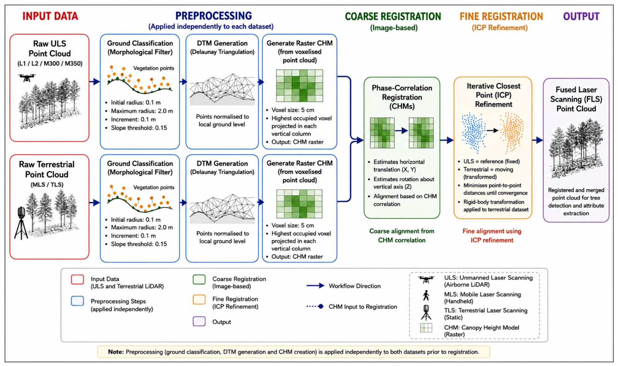
Processing Stage	Method	Parameter (s)
Ground classification	Progressive morphological filter	Initial radius 0.1 m; Maximum radius 2.0 m; Increment 0.1 m; Slope threshold 0.15
DTM generation	Delaunay triangulation	—
Height normalisation	DTM subtraction	—
CHM generation	Highest occupied voxel	5 cm voxel size
Coarse registration	Phase correlation	CHM-based
Fine registration	Iterative Closest Point (ICP)	Point-to-point
Reference dataset	ULS	Fixed
Moving dataset	MLS/TLS	Transformed
Output	Fused laser scanning (FLS)	Registered point cloud

.

Ground Classification: Ground points were identified using a progressive morphological filtering algorithm implemented in MATLAB 2026a. The filter employed an initial window radius of 0.1 m, increasing incrementally to a maximum radius of 2.0 m in 0.1 m steps. Elevation differences between successive windows were evaluated using a slope threshold of 0.15 to separate ground from vegetation. These parameters were selected empirically to provide stable ground classification across both radiata pine and eucalyptus plantations while preserving local terrain variation beneath dense forest canopies. Although alternative parameter combinations may be appropriate for other forest environments, the selected values produced consistent terrain models across all study sites.

Digital Terrain Model: Ground points were interpolated using Delaunay triangulation to generate a continuous digital terrain model (DTM). Point elevations within the original LiDAR datasets were subsequently normalised by subtracting the corresponding DTM elevation, producing point clouds referenced to local ground level. This normalisation ensured that tree heights derived from different acquisition platforms were directly comparable irrespective of local terrain variation.

Canopy Height Model: Normalised point clouds were first voxelised using a voxel size of 5 cm. The highest occupied voxel within each vertical column was then projected to generate a raster canopy height model (CHM). This approach reduced the influence of isolated outlier points while preserving local canopy maxima for subsequent image-based registration and tree detection.

Coarse Registration: Initial alignment between the ULS and terrestrial datasets was achieved using phase-correlation image registration applied to the corresponding canopy height models. Because both datasets had already been normalised to ground level, coarse registration was limited to horizontal translation and rotation about the vertical axis. This substantially reduced the search space for subsequent ICP refinement while avoiding the need for manually identified control points or accurately located tree stems.

ICP Refinement: Fine registration was performed using the Iterative Closest Point (ICP) algorithm, treating the ULS point cloud as the reference dataset and the terrestrial point cloud as the moving dataset. ICP iteratively minimised point-to-point Euclidean distances until convergence, producing the final rigid-body transformation required to align the datasets. The resulting transformation matrix was subsequently applied to the original terrestrial point cloud prior to point cloud fusion. The registered point clouds were subsequently merged to generate the FLS dataset used for tree detection and attribute extraction.

Unlike several forest registration workflows that require accurately surveyed tree locations or extensive manual intervention, the proposed approach relies only on independently generated canopy height models and automated ICP refinement. This makes the registration procedure readily transferable to production-scale plantation surveys while reducing dependence on site-specific control information.

2.5. Tree Detection, Attribute Extraction and Calibration-Transfer

Tree attributes from the high-density terrestrial and fused point clouds were extracted using the TreeLS package implemented in R (version 4.6.0) [101,102]. TreeLS performs individual-tree segmentation and stem reconstruction to estimate tree position and DBH. HT and CD were subsequently derived from the segmented tree point clouds. The high point density available within the MLS and FLS datasets enabled direct geometric reconstruction of tree stems, providing calibration-quality measurements that were subsequently used to evaluate and improve the ULS-derived estimates.

Within dense plantation forests, LiDAR penetration to the stem is limited, but returns that reach the stem generally exhibit both locally elevated point density and stronger return intensity than surrounding foliage. A local density–times–intensity map (LDTIM) exploits these complementary characteristics to enhance stem visibility within sparsely sampled ULS point clouds.

Point density is typically highest in the vicinity of tree stems, which also tend to exhibit stronger LiDAR return intensities than surrounding canopy elements. Accordingly, the number of returns within each vertical column associated with a raster cell was summed to generate a point-density model, while mean relative intensity values were calculated by averaging the intensity returns within the same columnar structure. The normalised density and intensity layers were then multiplied to produce a local density–intensity map, and a Gaussian smoothing filter was applied using a 5 × 5 kernel with a standard deviation of σ = 1 (full width at half maximum, FWHM ≈ 2.36 pixels).

It is acknowledged that the intensity measurements obtained from the L1 and L2 sensors were not radiometrically calibrated to account for range, incidence angle, or other acquisition-related effects. Consequently, absolute intensity values may vary across the flight strip. However, LDTIM relies primarily on relative intensity contrasts within local neighbourhoods rather than absolute intensity magnitudes. As a result, the combined local density x intensity metric provided a robust indicator of probable stem locations despite the absence of absolute radiometric calibration.

Individual tree crowns were segmented using a marker-controlled watershed algorithm [103] implemented in MATLAB. Tree-top detections were imposed as regional minima on the complement of the canopy height model using imimposemin, after which watershed segmentation was performed using 8-neighbour connectivity. Regions with canopy heights below 1 m were discarded and segments containing fewer than six pixels were removed before the remaining crowns were sequentially re-labelled.

Crown diameter (CD) was estimated from the projected crown area by calculating the diameter of an equivalent-area circle. Species-specific allometric regression models were then used to estimate DBH from HT and CD. Following González-Benecke et al. [65], DBH was estimated as

$$\mathrm{D}\mathrm{B}\mathrm{H}=\mathrm{e}\mathrm{x}\mathrm{p}\left({\beta }_0+{\beta }_1\mathrm{l}\mathrm{n}(\mathrm{H}\mathrm{T})+{\beta }_2\mathrm{l}\mathrm{n}\left[\pi {\left({\displaystyle \frac{\mathrm{C}\mathrm{D}}{2}}\right)}^2\right]\right)$$

Separate parameterisations were used for Pinus radiata and eucalyptus. Because a published parameterisation for Eucalyptus sieberi was unavailable in González-Benecke et al. [65], the E. globulus model was applied as a structural surrogate. This transfer represents a limitation and was subsequently evaluated through local calibration against TreeLS-derived DBH.

These models were selected because they were developed from extensive Chilean plantation datasets with structural characteristics similar to those of the plantations examined in this study and have reported adjusted coefficients of determination ($R_{Adj}^2$) of approximately 0.93–0.98, depending on species and predictor set. Alternative allometric models [62,104,105,106,107] were evaluated but generally produced larger prediction errors for the present datasets. Models incorporating stand density [63] were not considered and remain an avenue for future investigation. Published species-specific coefficients from González-Benecke et al. [65] were used without recalibration.

Stem Imputation Modelling: Use of FLS and ground-based LiDAR improves attribute extraction relative to ULS. However, such datasets are limited by the MLS plot size. Moreover, regression models, often the only viable approach for extracting stem parameters from sparser ULS point clouds, are often inadequate for commercial inventory operations.

Tree attributes were extracted from the FLS and terrestrial LiDAR datasets using the TreeLS package implemented in R. Because the study encompassed forest stands with markedly different canopy structures, tree sizes, and stem geometries, TreeLS processing parameters were adjusted for each forest type.

Parameters controlling stem mapping, voxelisation, circle fitting, and quality-control thresholds were selected following iterative optimisation to maximise stem reconstruction accuracy while minimising false detections. The final parameter sets used for each forest type are summarised in

Table 5. TreeLS processing parameters used for individual-tree segmentation, stem reconstruction, and DBH extraction. Parameter values were adjusted to accommodate differences in tree size, crown architecture, and stem geometry between tall radiata pine, medium radiata pine, and mature eucalyptus stands.

Parameter	Tall Radiata Pine	Medium Radiata Pine	Mature Eucalyptus
DBHWindow (m)	[1.15, 1.55]	[1.20, 1.45]	[1.10, 1.70]
TargetDBHHeight (m)	1.3	1.3	1.3
CrownMinHeight (m)	3	3	3
MapVoxelSizes (m)	[0.05, 0.075, 0.10, 0.15]	[0.10, 0.15, 0.20, 0.25]	[0.10, 0.15, 0.20, 0.25]
StemVoxelSize (m)	0.015	0.03	0.03
CircleTrimQuantile	0.6	0.28–0.35	0.65–0.75
FitRadiusLimits (m)	[0.06, 0.45]	[0.04, 0.22]	[0.08, 0.60]
RadiusRangeLoose (m)	[0.06, 0.40]	[0.08, 0.165]	[0.10, 0.60]
RadiusRangeClean (m)	[0.08, 0.35]	[0.09, 0.145]	[0.12, 0.50]
ErrorLooseBase (m)	0.1	0.08	0.12–0.14
ErrorLooseRadiusFactor	0.4	0.35	0.45–0.50
ErrorCleanMax (m)	0.08	0.05	0.10–0.12
RelErrorSuspect	0.55	0.35	0.60–0.70
ErrorSuspect (m)	0.1	0.1	0.12–0.14
LargeRadiusSuspect (m)	0.35	0.2	0.45–0.50
LargeRadiusErrorSuspect (m)	0.1	0.06	0.12–0.14
NLooseMin (count)	20	20	20
NCleanMin (count)	30	40	30–35
LowDensityN (count)	20	30	20–25
CleanMinTrees (count)	50	200	30–50
CleanMinFractionOfLoose	0.25	0.35	0.20–0.25

. A detailed description of the processing parameters is provided in the Supplementary Information.

To improve stem-attribute estimation across plantation areas observed only by ULS, a calibration-transfer framework was developed. First, the TreeLS package was applied to the FLS and ground-based MLS/TLS datasets to derive reference DBH estimates from the high-density point clouds. Second, these reference measurements were compared with DBH estimates obtained from the corresponding ULS component of the fused dataset (hereafter referred to as ULS_MLS [or ULS_TLS]) using the LDTIM and regression-based workflow. Third, statistical correction models were developed to transform the ULS_MLS regression estimates so that they more closely matched the TreeLS-derived reference values. Finally, the calibrated correction model was applied to the much larger ULS-only dataset (referred to as ULS_ALL) to generate improved DBH estimates across the entire plantation.

2.6. Statistical Imputation Methods

Several statistical approaches were evaluated to improve ULS-derived DBH estimates using the TreeLS-derived FLS measurements as the reference distribution. The methods ranged from simple distribution-matching techniques to conditional calibration models that incorporated the original ULS regression estimates. All methods were developed separately using the FLS and ground-based LiDAR calibration datasets and subsequently applied unchanged to the corresponding ULS-only datasets, thereby simulating a practical calibration-transfer workflow.

Direct Adjustment of Regression Model (Strategy 1): Empirical relationships between TreeLS estimates of DBH (derived from the FLS point cloud) and estimates of HT and CD (derived from LDTIM applied to the ULS_MLS data) were fitted to the regression model of [65] pertinent to each forest type/species so that model coefficients could be estimated using nonlinear least-squares optimisation. The data were first filtered to retain only trees with valid DBH, height, and crown measurements prior to model fitting. DBH values were then predicted for ULS_ALL using both HT and CD as explanatory variables based on the adjusted coefficients. During prediction, tree height and crown diameter values were constrained to biologically realistic ranges derived from the training data to reduce extreme extrapolation behaviour.

Weighted Adjustment of Regression Model (Strategy 2): In this strategy, model coefficients were again estimated using nonlinear least-squares optimisation, but with a 90% weight towards the original coefficients of [65]. The training data were again filtered to retain only trees with valid DBH, height, and crown measurements prior to model fitting. Constraints to biologically realistic predictor ranges were not required for this approach.

CDF with Two Beta Functions (Strategy 3): In this strategy, the DBH for each tree within FLS was computed using TreeLS and a beta distribution, ${y_{TreeLS}=\beta }_{TreeLS}\left(x_{TreeLS}\right)$, fitted to this data, where $x_{TreeLS}$ is the sample data and $y_{TreeLS}$ the CDF value associated with each DBH value, $x_{TreeLS}$.

A probability density function (PDF) describes the relative likelihood that a continuous random variable takes values within different regions of its domain. Unlike a discrete probability mass function, the PDF does not represent the probability of an exact value; instead, probabilities are obtained by integrating the PDF over an interval. The cumulative distribution function (CDF) gives the probability that a random variable is less than or equal to a specified value. For continuous variables, the CDF is obtained by integrating the PDF and, provided it is monotonic, may be uniquely inverted.

The goal of the imputation strategies is thus to adjust the CDF of the ULS_MLS regression model to match the TreeLS estimates and then apply the corrections to the ULS_ALL region, to which only regression models can be applied. The inverse of the corrected CDF may then be used to compute better attribute values for this (larger and sparser) region.

LDTIM was used to determine the location of every tree in the ULS_ALL dataset and the regression model of [65] used to calculate their corresponding DBH values. A second beta function, ${y_{ULS\_ALL}=\beta }_{ULS\_ALL}\left(x_{ULS\_ALL}\right)$, was fitted to this dataset and the CDF values, $y_{ULS\_ALL}$, again calculated for each of the regression estimates of DBH, $x_{ULS\_ALL}$. Using the ${\beta }_{TreeLS}$ distribution, the inverse values of the distribution probabilities were then evaluated at each CDF value of the ULS_ALL regression estimates used to form ${\beta }_{ULS\_ALL}$ (i.e., $x_{ULS\_ALL}$), so $x_{imp}={\beta }_{TreeLS}^{-1}\left({\beta }_{ULS\_ALL}\left(x_{ULS\_ALL}\right)\right)$, where $x_{imp}$ are the imputed values for the ULS_ALL dataset.

CDF with Other Functions (Strategies 4–7): In these strategies, the beta functions were simply replaced by Weibull, Nakagami, Normal, and Log-Normal distributions, and the imputation processing described in Strategy 3 repeated.

Empirical Quantile Mapping (Strategy 8): In this strategy, empirical quantile mapping was implemented as a deterministic distribution-matching procedure that required neither model fitting nor predictor standardisation. ULS trees were ranked according to their regression-derived DBH estimates, and empirical percentile positions were calculated using MATLAB’s tiedrank function, which assigns average ranks to tied observations using $p_i={\displaystyle \frac{\mathrm{t}\mathrm{i}\mathrm{e}\mathrm{d}\mathrm{r}\mathrm{a}\mathrm{n}\mathrm{k}\left(x_i\right)}{n+1}},$ where $x_i$ is the regression-derived DBH of tree $i$.

The corresponding empirical quantiles of the TreeLS DBH reference distribution (derived from either the FLS or ground-based LiDAR calibration data) were then assigned to each ULS tree using ${\mathrm{D}\mathrm{B}\mathrm{H}}_{\mathrm{i}\mathrm{m}\mathrm{p}\mathrm{u}\mathrm{t}\mathrm{e}\mathrm{d}}=Q_{\mathrm{T}\mathrm{r}\mathrm{e}\mathrm{e}\mathrm{L}\mathrm{S}}\left(p_i\right),$ where $Q_{\mathrm{T}\mathrm{r}\mathrm{e}\mathrm{e}\mathrm{L}\mathrm{S}}$ denotes the empirical quantile function of the calibration distribution.

This approach preserved the rank ordering of the original ULS regression DBH estimates while forcing the final DBH distribution to match the empirical TreeLS reference distribution. The method did not use additional structural predictors, spatial matching, nearest neighbours, regression residuals, or stochastic sampling.

Bias-Corrected Conditional Rank–Quantile Blending (Strategy 9): For this strategy, a study-developed hybrid calibration procedure was used to combine bias correction, weighted conditional regression, and empirical rank–quantile mapping. The approach incorporated rank-based distribution-mapping principles [108], but extended them by first adjusting the ULS regression-derived DBH predictor and then using additional structural attributes to derive a conditional ranking of the target trees. This ranking was subsequently mapped to the TreeLS-derived reference DBH distribution and blended with the conditional-mean predictions.

Before model fitting, a constant additive correction was applied to the ULS regression-derived DBH values. Candidate bias values ranging from −5 to 5 cm in 0.1 cm increments were evaluated, and the value that minimised the mean DBH difference among candidate TreeLS–ULS matches was selected. The corrected ULS DBH values were then used both in the calibration matching procedure and as predictors in the subsequent regression model.

Candidate correspondences between TreeLS stems and ULS-detected tree apexes were identified within a maximum horizontal distance of 3.0 m. Each candidate match was assigned a combined Gaussian weight based on spatial separation and DBH similarity, using scale parameters of ${\sigma }_{XY}=1.0$m and ${\sigma }_{\mathrm{D}\mathrm{B}\mathrm{H}}=5.0$cm. Matches with combined weights of 0.01 or less were discarded.

A weighted linear regression model was fitted using TreeLS-derived DBH as the response and bias-corrected ULS regression DBH, tree height, crown area, and the interaction between ULS DBH and tree height as predictors, ${\mathrm{D}\mathrm{B}\mathrm{H}}_{\mathrm{T}\mathrm{r}\mathrm{e}\mathrm{e}\mathrm{L}\mathrm{S}}\sim {\mathrm{D}\mathrm{B}\mathrm{H}}_{\mathrm{U}\mathrm{L}\mathrm{S}}+\mathrm{H}\mathrm{T}+\mathrm{C}\mathrm{A}+{\mathrm{D}\mathrm{B}\mathrm{H}}_{\mathrm{U}\mathrm{L}\mathrm{S}}\times \mathrm{H}\mathrm{T}.$

The fitted conditional-mean predictions were used to rank the ULS trees. Empirical probability positions derived from these ranks were then mapped onto the TreeLS reference DBH distribution. Final predictions comprised 80% quantile-mapped DBH and 20% scaled conditional-mean DBH. Negative values were truncated to zero, and a final additive correction aligned the mean of the positive imputed values with the TreeLS reference mean.

Conditional Rank–Quantile Blending (Strategy 10): This strategy used the same weighted conditional-regression and empirical rank-mapping framework as Strategy 9, but without the initial additive bias correction to the ULS regression-derived DBH predictor. Candidate TreeLS–ULS matches were identified within 3.0 m and weighted according to horizontal distance and DBH similarity using Gaussian scale parameters of 1.0 m and 5.0 cm, respectively. Matches with combined weights of 0.01 or less were excluded.

A weighted linear regression model was fitted using TreeLS-derived DBH as the response and ULS regression DBH, tree height, crown area, and the interaction between ULS DBH and tree height as predictors. The fitted conditional-mean estimates were converted to empirical ranks and mapped onto the TreeLS DBH reference distribution. Final predictions combined 80% quantile-mapped DBH with 20% scaled conditional-mean DBH, after which negative values were truncated to zero and an additive correction aligned the imputed mean with the TreeLS reference mean.

Regression residuals were calculated during model fitting but were not sampled or reintroduced into the final predictions. Therefore, this strategy should not be interpreted as residual-spread restoration.

Voxel-Based Imputation (Strategy 11): The final strategy, a voxel-based regression model, was developed to estimate DBH from whole-tree three-dimensional structural metrics derived from the ULS point clouds. Each segmented tree point cloud was voxelised at a resolution of 0.25 m. The resulting tree-level predictors comprised tree height, crown diameter, crown area, occupied voxel volume, number of occupied voxels, and the 25th, 50th, 75th, and 90th percentiles of the vertical point distribution: HT, CD, CA (crown projected area), V_voxel (total volume occupied by filled voxels within the segmented tree in m³), N_voxel (number of occupied voxels), Z₂₅ (25th percentile of LiDAR point heights within the tree), Z₅₀ (median LiDAR point height), Z₇₅ (75th percentile of LiDAR point height), and Z₉₀ (90th percentile of LiDAR point height).

Only predictors available in the calibration-source, local ULS, and complete ULS datasets were retained. Predictor variables were standardised using the mean and standard deviation calculated from the combined predictor space of the calibration-source and local ULS datasets. This shared standardisation was used to place the dense and aerial observations within a common structural feature space.

TreeLS-derived DBH values were assigned to the corresponding calibration voxel trees using nearest-neighbour matching of horizontal tree coordinates. Local ULS trees were then matched to their nearest calibration-source tree in the standardised voxel-predictor space using $K=1$. Matches with distances greater than the 90th percentile of all matching distances were excluded to reduce the influence of structurally dissimilar calibration pairs.

A bagged regression-tree ensemble was fitted using MATLAB’s fitrensemble function with the bagging method. The individual tree learners used a minimum leaf size of four and surrogate splits were disabled. The implemented model used 100 learning cycles. The retained local ULS predictor rows formed the training predictors, while the TreeLS-derived DBH values transferred from their matched calibration trees formed the training targets.

The fitted ensemble was then applied to the complete ULS dataset to obtain initial DBH predictions. To avoid excessive compression of the upper tail, predictions above the 75th percentile received an additional stochastic perturbation drawn from a Gaussian distribution with standard deviation equal to 20% of the training-residual standard deviation.

Residual-spread restoration was then applied. For each target tree, the five nearest training observations were identified in standardised predictor space. One residual was randomly sampled from these neighbours and added to the ensemble prediction. Residual donors could be selected for more than one target tree, equivalent to sampling with replacement across predictions. A fixed random seed of 1 was used to ensure reproducibility.

The resulting predictions were subsequently subjected to a sequence of distributional corrections. These comprised median uplift, soft tapering towards the 1st and 99th percentiles of the TreeLS DBH reference distribution, quantile adjustment at probabilities of 0.05, 0.25, 0.50, 0.75, and 0.95, application of a capped multiplicative mean-adjustment factor, and a final shift towards the TreeLS reference mean using a mean-correction strength of 1.35. The final estimates therefore combined structurally informed ensemble prediction, local residual restoration, and distributional calibration to preserve both tree-level structural relationships and realistic stand-level DBH variability.

The principal properties of the eleven calibration and imputation strategies are summarised in

Table 6. Summary of the method classes evaluated for transferring TreeLS-derived DBH information from fused or ground-based LiDAR calibration plots to ULS-only plantation areas.

Strategy	Calibration or Imputation Method	Targets Mean Bias	Targets Distribution Spread	Targets Full Distribution Shape	Ranking Used for Distribution Mapping	Uses Structural Predictors
1	Direct adjustment of allometric regression model	✓	Approx.	✗	Generally	HT, CD
2	Weighted adjustment of allometric regression model	✓	Approx.	✗	Generally	HT, CD
3	Beta-distribution CDF mapping	✓	✓	Approx.	Original DBH ranking	✗
4	Weibull-distribution CDF mapping	✓	✓	Approx.	Original DBH ranking	✗
5	Nakagami-distribution CDF mapping	✓	✓	Approx.	Original DBH ranking	✗
6	Normal-distribution CDF mapping	✓	✓	Approx.	Original DBH ranking	✗
7	Log-normal-distribution CDF mapping	✓	✓	Approx.	Original DBH ranking	✗
8	Empirical quantile mapping	✓	✓	✓	Original DBH ranking	✗
9	Bias-corrected conditional quantile mapping	✓	✓	✓	Conditional model ranking	DBH, HT and CA
10	Conditional quantile mapping	✓	✓	✓	Conditional model ranking	DBH, HT and CA
11	Voxel-based ensemble imputation with residual and quantile adjustment	✓	✓	Approx. to ✓	Not explicitly constrained/general	HT, CD, CA, voxel metrics

. The methods differed in whether they primarily corrected mean bias, restored distributional spread, matched the complete reference distribution, preserved the original ordering of trees, or incorporated tree-level structural predictors [note for Table 6: “✓” indicates that the method explicitly targets the stated property; “✗” indicates no; “Approx.” indicates that the property is reproduced indirectly or approximately rather than being constrained exactly; “Generally” indicates that monotonicity of the fitted allometric relationship will usually preserve relative ordering, although this is not guaranteed under all predictor combinations. The full-distribution performance of voxel-based imputation depends on the subsequent residual-spread restoration and quantile-adjustment steps]. For all strategies, regression model corrections were obtained from TreeLS detections and stem segmentations applied to (i) the FLS point clouds and (ii) ground-based LiDAR data alone.

The objective of comparing multiple imputation strategies was not simply to minimise numerical error, but to determine which methods most effectively reproduced the TreeLS-derived reference DBH distribution while improving agreement with the field-observed stand mean. This distinction is particularly important for commercial plantation inventory, where realistic stand structure is generally more valuable than exact prediction for individual stems.

2.7. Validation and Statistical Analysis

The proposed calibration-transfer framework was evaluated exclusively at the stand level. The primary objective was to determine whether the statistical correction methods improved the representation of stand-level DBH distributions derived from ULS data, rather than to predict the exact diameter of individual trees. Consequently, model performance was assessed using measures of central tendency, variability, distributional agreement, and graphical comparison. Statistical significance was interpreted alongside effect sizes and confidence intervals to distinguish practically meaningful improvements from differences arising solely from large sample sizes.

Field measurements provided an independent reference for evaluating stand-level DBH statistics. TreeLS-derived DBH estimates obtained from the calibration plots were used to construct statistical calibration models but were not themselves treated as independent validation data. Validation therefore focused on comparing stand-level summaries and distributions of the corrected ULS estimates against available field observations.

For each imputation method, stand-level summary statistics, including mean, median, standard deviation, and other descriptive measures, were calculated and compared with the corresponding field observations. Distributional agreement between imputed and observed DBH values was assessed using graphical and statistical techniques. Confidence intervals and effect sizes were reported alongside hypothesis tests to facilitate interpretation of practical significance.

Graphical comparisons included boxplots and other distributional summaries. These visualisations were used to assess the extent to which each imputation method improved agreement with the field-observed stand mean while producing DBH distributions calibrated to the TreeLS-derived reference distribution.

For each imputation strategy, the distribution of predicted DBH was compared with the corresponding field-observed stand mean. Stand-level summary statistics included the imputed mean, median, standard deviation, mean difference, absolute bias, and absolute relative error. The mean difference was calculated as the imputed mean minus the field mean; negative values therefore indicate underestimation and positive values indicate overestimation. Absolute bias was expressed in centimetres, while absolute relative error was expressed as a percentage of the field mean.

For completeness, for each imputation strategy, the mean predicted DBH was compared with the corresponding field-observed stand mean using a two-sided one-sample t-test, with the imputed DBH values treated as the sample and the field mean treated as a fixed reference value. Because a non-significant difference test does not establish agreement, practical equivalence was additionally assessed using the two one-sided tests (TOST) procedure. Equivalence bounds were prespecified as ±1.0 cm around the field-reference mean, representing the maximum stand-level mean DBH difference considered practically negligible for the purposes of this study. Equivalence was concluded only when both one-sided tests were significant at $\alpha =0.05$, equivalent to the 90% confidence interval for the mean difference lying wholly within the equivalence bounds. Because the imputed values are model outputs rather than independent field observations and uncertainty in the field-reference mean is not fully propagated, both the one-sample test and TOST were interpreted as supplementary stand-level assessments and were not used as the primary basis for ranking the calibration strategies.

The magnitude of the remaining stand-level bias was quantified using bias-corrected Hedges’ g—a standardised measure of residual bias—calculated from the standardised mean difference. Absolute Hedges’ g values were interpreted using conventional thresholds: negligible (<0.20), small (0.20–<0.50), moderate (0.50–<0.80), and large (≥0.80).

Additional statistical results, including complete summary statistics for all calibration strategies, confidence intervals, effect sizes, and graphical comparisons of DBH distributions for every forest type and calibration source, are provided in the Supplementary Information.

The overall workflow therefore consists of five stages: (1) acquisition of complementary aerial and terrestrial LiDAR, (2) generation of fused calibration datasets, (3) extraction of TreeLS-derived calibration attributes within the calibration region, (4) learning statistical relationships between dense and sparse structural observations, and (5) transferring those relationships to the surrounding ULS-only area to recover realistic stand-level inventory distributions.

3. Results

3.1. Attribute Extraction

Pine Trees: Distribution means for HT, DBH, and CD (±one standard deviation) extracted from the pine datasets using LDTIM for HT and CD and the regression model of [65] for DBH are summarised in

Table 7. Stand-level summary statistics (mean ± standard deviation) for tree height (HT), crown diameter (CD), and diameter at breast height (DBH) extracted from the various LiDAR datasets, together with corresponding field observations for the radiata pine site. DBH was derived using the regression model of [65].

Attribute	ULS High Res.	ULS Low Res.	MLS	FLS	Field Measurements
					95% CI	Mean ± SD
	All Tall Trees
HT (m)	20.8 ± 3.7	19.8 ± 3.0	19.8 ± 5.0	20.8 ± 3.8	20.0–20.9	20.5 ± 1.6
CD (m)	4.6 ± 0.4	4.7 ± 1.5	4.4 ± 0.9	4.5 ± 0.4	2.5–2.9	2.7 ± 0.6
DBH (cm)	27.4 ± 3.1	27.9 ± 0.4	27.5 ± 3.9	27.7 ± 3.0	24.1–26.9	25.5 ± 5.3
	All Medium Trees
HT (m)	11.2 ± 2.4	11.1 ± 2.5	11.0 ± 2.7	11.3 ± 1.9	11.0–11.8	11.4 ± 1.1
CD (m)	3.1 ± 0.4	3.1 ± 0.5	3.1 ± 0.8	3.1 ± 0.7	1.9–2.5	2.2 ± 0.4
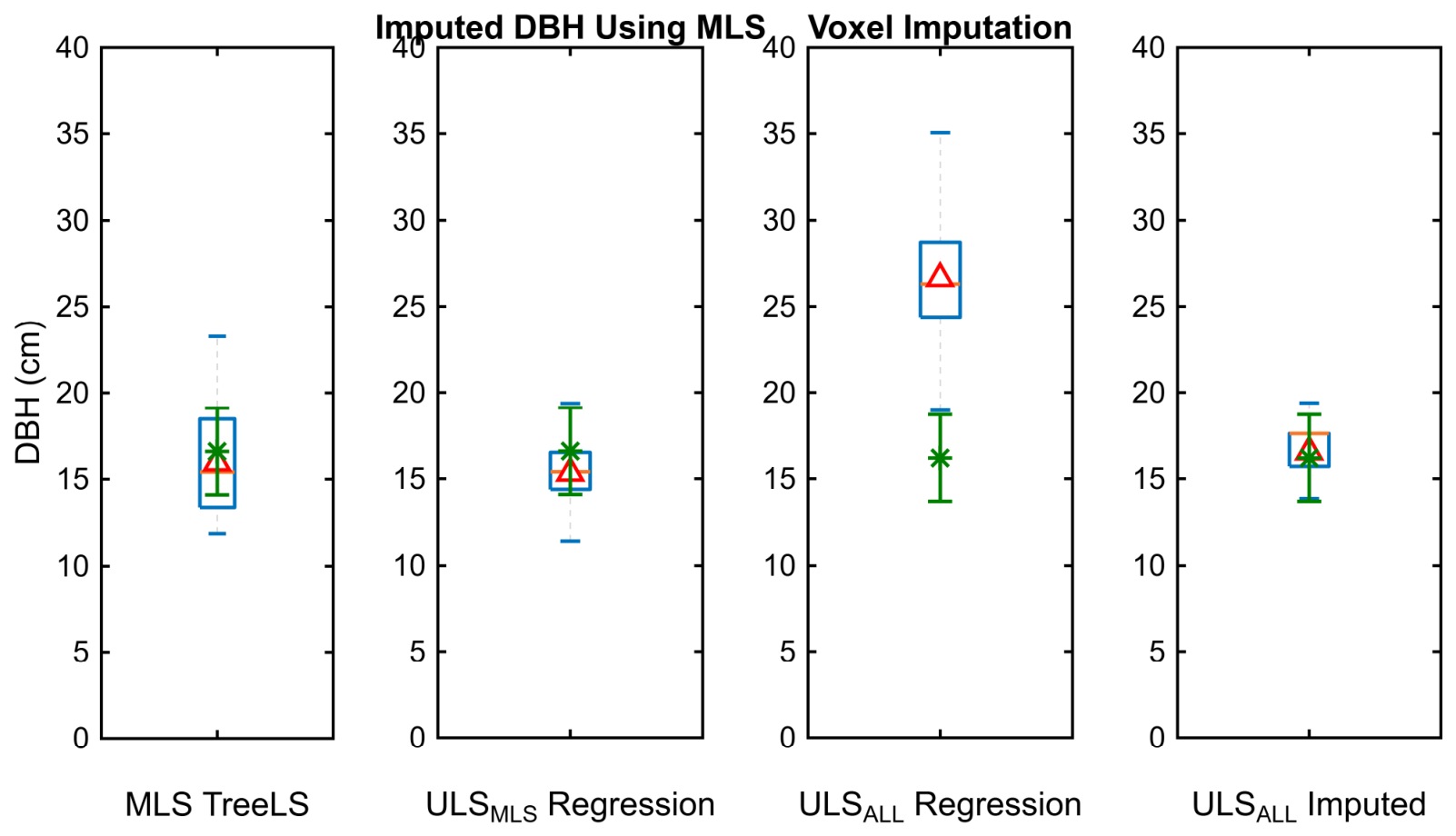
DBH (cm)	26.6 ± 5.2	26.2 ± 5.3	15.3 ± 3.7	26.9 ± 3.9	15.6–17.2	16.2 ± 2.5

. The distributions of the parameters were drawn only from trees identified by LDTIM with >1000 points.

Tree-height estimates from ULS, FLS, and ground-based LiDAR therefore showed the expected level of agreement and were sufficiently accurate to support subsequent DBH modelling. As tree height served primarily as a predictor within the regression and calibration-transfer framework, rather than as a standalone response variable, detailed evaluation focused on its suitability as an input to DBH estimation. Consequently, the principal performance assessment presented in the Results concerns the accuracy of the derived DBH distributions rather than tree-height estimates themselves.

The mean height of all 55 tall trees measured using traditional field techniques was 20.5 ± 1.6 m, indicating good alignment between the field measurements and LDTIM-derived heights obtained from the ULS and FLS datasets. As might be expected—and probably due to canopy occlusion—the mean height obtained from the MLS point clouds is slightly low. The mean heights also show good correspondence for the medium-sized trees, with the MLS estimates again slightly low.

Crown diameters extracted from the LiDAR point clouds were consistently larger than the corresponding field observations.

Despite this, the regression-derived DBH estimates have means of 27.4 ± 3.1 cm, 27.9 ± 0.4 cm, 27.5 ± 3.9 cm, and 27.7 ± 3.0 cm for the tall trees ULS (high resolution), ULS (low resolution), MLS, and FLS datasets, respectively. Most estimates exceeded the field-observed mean DBH for both tall and medium radiata pine stands (noting the MLS-based estimates did not), indicating systematic bias prior to calibration. DBH estimates for the medium trees were 26.6 ± 5.2 cm, 26.2 ± 5.3 cm, 15.3 ± 3.7 cm, and 26.9 ± 3.9 cm for the ULS (high resolution), ULS (low resolution), MLS, and FLS data, respectively (Table 7).

Table 8. Comparison of TreeLS-derived reference DBH and regression-derived DBH estimates for the calibration (MLS/FLS) and operational (ULS-only) datasets.

Tree Set	TreeLS Model			Regression Model			Field Measurements
	ULS	MLS	FLS	ULS	MLS	FLS
Calibration-region (tall trees)	-	24.9	24.4	27.4	27.5	27.2	25.4 ± 5.3
Target-region (tall trees) ULS-only data	-	-	-	27.7	-	-	25.6 ± 2.7
Calibration-region (medium-sized trees)	-	15.9	17.7	26.6	12.5	26.9	16.6 ± 1.3
Target-region trees (medium) ULS-only data	-	-	-	26.6	-	-	16.2 ± 2.3

shows a summary of distribution means for DBH extracted from the FLS and ULS_ALL datasets using TreeLS and LDTIM for HT and CD and the regression model of [65] for DBH, respectively. As expected, the regression model did not estimate DBH as accurately as TreeLS, likely due to insufficient complex internal structure in the ULS_ALL data for TreeLS to function properly, and there is no MLS data to process in these regions.

Eucalyptus Trees: A single set of DBH field measurements was obtained for the eucalyptus site in Tasmania, the mean of which was 36.9 ± 8.8 cm. Distribution means of 34.4 cm (L1 ULS), 37.8 cm (L2 ULS), 37.5 cm (TLS), 41.3 cm (L1 FLS), and 42.0 cm (L2 FLS) were obtained using TreeLS (

Table 9. Mean of field measurements for eucalyptus trees and attributes extracted using TreeLS. Due to time constraints tree height and crown diameter were not measured in the field, so no direct field-based validation of LiDAR-derived estimates was possible.

Attribute	L1 ULS	L2 ULS	TLS	L1 FLS	L2 FLS	Field Measurements
HT (m)	32.1 ± 2.8	32.4 ± 3.0	30.9 ± 5.0	31.9 ± 3.8	32.2 ± 3.8	--
CD (m)	6.5 ± 0.4	9.6 ± 1.5	5.9 ± 0.9	6.0 ± 0.4	10.2 ± 3.8	--
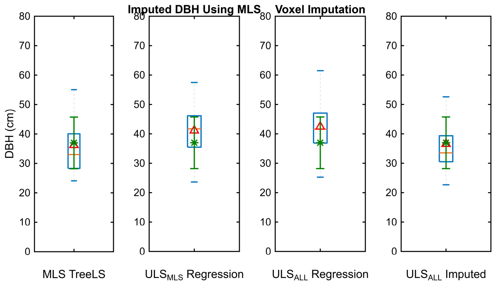
DBH (cm)	34.4 ± 3.1	37.8 ± 0.4	37.5 ± 3.9	41.3 ± 3.0	42.0 ± 3.8	36.9 ± 8.8

). Although the total tree heights were not measured in the field, it is noted that, once again, those derived using the TLS data are lower than the ULS measurements (note: the smaller (6 m), 3-year-old Tasmanian blue gums (Eucalyptus globulus) were not analysed in this study).

DBH estimates derived from the L2 ULS dataset were closer to the field-observed mean than those obtained from the L1 dataset, whereas the FLS datasets tended to overestimate stand mean DBH (Table 9).

Because ground-based LiDAR provided the densest and geometrically cleanest observations of stem surfaces, TreeLS-derived estimates from these datasets were treated as the structural calibration reference rather than as independent validation measurements.

3.2. Imputation Results

DBH distributions for the tall and medium pine and eucalyptus plantations are shown in Figure 4, Figure 5 and Figure 6. The sub-plots in each figure show: (left) TreeLS applied to the ground-based LiDAR calibration data, (centre-left) the regression model applied to the ULS component of the LiDAR calibration dataset, (centre-right) the regression model applied to the entire ULS dataset, and (right) voxel-based imputation applied to ULS dataset for the whole site (ULS_ALL).

All DBH distribution boxplots were derived from approximately equal sample sizes (N ≈ 300 trees per group for the pine and 120 for the eucalyptus). Although sample size labels are not shown directly on the figures (see Supplementary Material), the distributions are therefore broadly comparable in terms of statistical representation.

In each boxplot, the mean of the distribution is shown as a red triangle, the centreline and the lower and upper edges each box indicate the median, 25th, and 75th percentiles, respectively, while the lower and upper whiskers the indicate the extrema. The green asterisks show the means of the relevant field observations, and the green error bars on either side of the asterisks represent ± one standard deviation from the mean of the field observations.

The imputed distributions in Figure 4, Figure 5 and Figure 6, were generated using models calibrated from TreeLS-derived DBH estimates obtained from the ground-based LiDAR datasets rather than the corresponding FLS datasets. The means of the field measurements were 25.5 ± 5.3 cm, 16.2 ± 2.5 cm, and 36.9 ± 8.8 cm, for the tall and medium pine and eucalyptus, respectively. The means of the regression model estimates without imputation were 27.4 cm, 26.6 cm, and 42.4 cm, for the tall and medium pine and eucalyptus, respectively, representing 8%, 64%, and 15% errors, respectively.

The means of the best imputed distributions based on MLS training were 25.5 cm (voxel-based), 16.5 cm (voxel-based), and 36.5 cm (voxel-based). These represent errors of approximately 2% or less. To maintain a concise presentation of the principal findings,

Table 10. Mean imputation estimates of DBH for tall and medium pine and mature eucalyptus plantations based on FLS training data. The values in parentheses are absolute differences from the field measurements, which are for ULS_ALL regions. Values are coloured blue if they are low and red if they are high.

Observation or Imputation Strategy	Tree Set and DBH in cm (and Errors)
	Radiata Pine		Eucalyptus	Comments
	Tall	Medium	Tall
Field Observations	25.5 ± 5.3	16.2 ± 2.5	36.9 ± 8.8	Reference distribution
Direct Adjustment of Model Mean bias correction	26.9 (1.4)	17.1 (0.9)	33.7 (3.2)	Simple bias correction
Weighted Adjustment of Model Weighted mean correction	30.1 (4.6)	23.8 (7.6)	39.7 (2.8)	Inconsistent
Beta Function CDFs Parametric distribution matching	24.4 (1.1)	17.4 (1.2)	37.2 (0.3)	Robust matching
Weibull Function CDFs Parametric distribution matching	24.5 (1.0)	18.0 (1.7)	36.3 (0.6)	Strong performance for eucalyptus
Nakagami Function CDFs Parametric distribution matching	24.4 (1.1)	17.8 (1.6)	36.5 (0.4)	Comparable to Weibull for Eucalyptus
Normal Function CDFs Parametric distribution matching	24.4 (1.1)	17.8 (1.6)	37.7 (0.8)	Stable performance for both species
Log-Normal Function CDFs Parametric distribution matching	24.4 (1.1)	17.8 (1.6)	37.5 (0.6)	Stable performance for both species
Empirical Quantile Mapping Non-parametric distribution matching	24.4 (1.1)	17.8 (1.6)	37.5 (0.6)	Good distribution matching
Bias-Corrected Conditional Rank–Quantile Blending Rank-preserving distribution mapping	24.4 (1.1)	17.8 (1.6)	37.8 (0.9)	Preserves distributional ranking
Conditional Rank–Quantile Blending Effective and stable conditional and distributional calibration	24.4 (1.1)	17.8 (1.6)	37.8 (0.9)	Combines conditional structural ranking with distribution calibration
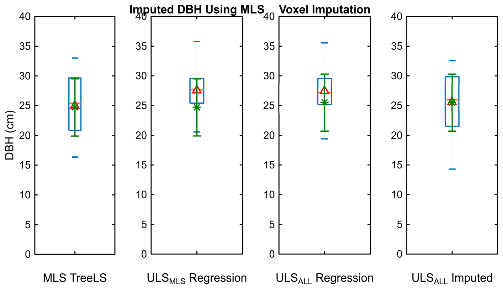
Voxel-Based Imputation Spatially informed calibration	24.6 (0.9)	17.6 (1.4)	39.2 (2.3)	Strongest performance for pine
Regression Model No Imputation	27.4 (1.9)	26.6 (10.4)	42.4 (5.5)	Uncorrected baseline

and

Table 11. Mean imputation estimates of DBH for tall and medium pine and mature eucalyptus plantations based on ground-based LiDAR (MLS/TLS) training data. The values in parentheses are differences from the field measurements, which are for ULS_ALL regions. Values are coloured blue if they are low and red if they are high.

Observation or Imputation Strategy	Tree Set and DBH in cm (and Errors)
	Radiata Pine		Eucalyptus	Comments
	Tall	Medium	Tall
Field Observations	25.5 ± 5.3	16.2 ± 2.5	36.9 ± 8.8	Reference distribution
Direct Adjustment of Model Mean bias correction	25.8 (0.3)	13.7 (2.5)	38.9 (2.0)	Moderate improvement
Weighted Adjustment of Model Weighted mean correction	28.6 (3.1)	22.5 (6.3)	44.1 (7.2)	Inconsistent
Beta Function CDFs Parametric distribution matching	24.8 (0.6)	16.5 (0.3)	36.3 (0.6)	Robust Matching
Weibull Function CDFs Parametric distribution matching	25.1 (0.4)	16.0 (0.2)	34.6 (2.3)	Strong performance for medium pine
Nakagami Function CDFs Parametric distribution matching	24.9 (0.6)	16.0 (0.2)	35.2 (1.7)	Stable performance for both species
Normal Function CDFs Parametric distribution matching	24.9 (0.6)	16.0 (0.2)	35.0 (1.9)	Stable performance for both species
Log-Normal Function CDFs Parametric distribution matching	25.0 (0.5)	16.0 (0.2)	36.0 (0.9)	Stable performance for both species
Empirical Quantile Mapping Non-parametric distribution matching	24.9 (0.6)	15.9 (0.3)	36.0 (0.9)	Robust non-parametric calibration
Bias-Corrected Conditional Rank–Quantile Blending Rank-preserving distribution mapping	24.9 (0.6)	15.9 (0.3)	36.1 (0.8)	Good preservation of distribution shape
Conditional Rank–Quantile Blending Effective and stable conditional and distributional calibration	24.9 (0.6)	15.9 (0.3)	36.1 (0.8)	Effective Stable conditional & distributional calibration
Voxel-Based Imputation Spatially informed calibration	25.5 (0.0)	16.5 (0.3)	36.5 (0.4)	Excellent for pine; competitive for eucalyptus
Regression Model No Imputation	27.4 (1.9)	26.6 (10.4)	42.4 (5.5)	Uncorrected baseline

summarise the key performance metrics for every calibration strategy, forest type, and calibration source. Complete statistical summaries for all calibration strategies, together with graphical comparisons of the resulting DBH distributions for each forest type and calibration source, are provided in the Supplementary Information.

Because individual field observations of accurate tree locations were unavailable, statistical testing was performed against reported field summary statistics rather than paired tree-level measurements. Consequently, the analysis evaluates stand-level mean agreement, supported by field summary statistics; distribution-shape calibration was evaluated principally relative to TreeLS-derived reference distributions.

Overall, the calibration-transfer framework substantially reduced stand-level DBH bias across all forest types. The largest improvement occurred for the medium radiata pine stands, where the mean DBH error decreased from approximately 10.4 cm (approximately 64%) for the uncorrected regression model to approximately 0.2–1.4 cm following calibration, depending on the imputation strategy employed. Comparable improvements were observed for the tall radiata pine and mature eucalyptus stands, demonstrating that the framework consistently reduced systematic stand-level bias.

Regarding

Table 12. Stand-level statistical comparison of FLS-trained calibration methods for tall radiata pine. Absolute Hedges’ g values were interpreted using conventional thresholds: negligible (<0.20), small (0.20–<0.50), moderate (0.50–<0.80), and large (≥0.80).

Strategy	Imputed Mean (cm)	Absolute Bias (cm)	95% CI for Mean Difference (cm)	Hedges’ g	Practical Importance
Direct Adjustment	26.88	1.38	1.25 to 1.51	0.889	Large
Weighted Adjustment	30.09	4.59	4.31 to 4.87	1.362	Large
Beta CDF	24.44	1.06	−1.54 to −0.59	−0.246	Small
Weibull CDF	24.54	0.96	−1.32 to −0.60	−0.225	Small
Nakagami CDF	24.41	1.09	−1.48 to −0.70	−0.233	Small
Normal CDF	24.42	1.08	−1.60 to −0.57	−0.231	Small
Log-Normal Mapping	24.42	1.08	−1.60 to −0.57	−0.231	Small
Empirical Quantile Mapping	24.41	1.09	−1.59 to −0.59	−0.241	Small
Bias-Corrected Conditional Rank–Quantile Blending	24.41	1.09	−1.59 to −0.59	−0.242	Small
Conditional Rank–Quantile Blending	24.41	1.09	−1.58 to −0.60	−0.243	Small
Voxel-Based Imputation	24.59	0.91	−1.22 to −0.60	−0.210	Small

and

Table 13. Stand-level statistical comparison of MLS-trained calibration methods for tall radiata pine. Absolute Hedges’ g values were interpreted using conventional thresholds: negligible (<0.20), small (0.20–<0.50), moderate (0.50–<0.80), and large (≥0.80).

Strategy	Imputed Mean (cm)	Absolute Bias (cm)	95% CI for Mean Difference (cm)	Hedges’ g	Practical Importance
Direct Adjustment	25.81	0.31	0.26 to 0.35	0.529	Moderate
Weighted Adjustment	28.64	3.14	2.91 to 3.37	1.135	Large
Beta CDF	24.81	0.69	−1.19 to −0.18	−0.148	Negligible
Weibull CDF	25.11	0.39	−0.77 to −0.01	−0.085	Negligible
Nakagami CDF	24.94	0.56	−1.00 to −0.13	−0.109	Negligible
Normal CDF	24.94	0.56	−0.99 to −0.13	−0.109	Negligible
Log-Normal Mapping	24.95	0.55	−1.12 to 0.03	−0.105	Negligible
Empirical Quantile Mapping	24.94	0.56	−1.11 to −0.01	−0.112	Negligible
Bias-Corrected Conditional Rank–Quantile Blending	24.94	0.56	−1.10 to −0.02	−0.114	Negligible
Conditional Rank–Quantile Blending	24.94	0.56	−1.10 to −0.02	−0.113	Negligible
Voxel-Based Imputation	25.54	0.04	−0.30 to 0.38	0.009	Negligible

, because the imputed values are model outputs and the field reference was available as a stand summary rather than matched individual-tree observations, inferential statistics are supplementary and do not constitute individual-tree validation.

The eleven methods formed three broad classes. Direct regression adjustment improved mean bias but generally failed to reproduce the observed distribution. Distribution-matching approaches (Strategies 3–10) consistently reduced bias and restored realistic stand-level variability, with relatively small differences among the individual distribution models. Voxel-based imputation generally provided the most accurate and consistent results, particularly for radiata pine, suggesting that explicit representation of three-dimensional tree structure provides additional predictive information beyond distributional correction alone.

From a routine inventory perspective, recovery of realistic stand-level DBH distributions is arguably more important than perfect prediction of individual trees because many management decisions rely on stand summaries, diameter distributions, biomass estimates, and yield forecasts rather than the attributes of specific stems.

4. Discussion

The principal contribution of this study is not a new stem reconstruction algorithm, but a calibration-transfer framework that enables structurally accurate information derived from relatively small terrestrial LiDAR surveys to improve stand-level inventories over much larger aerially surveyed areas.

This study demonstrates that fusion of ULS and ground-based LiDAR point clouds improved structural completeness, georeferencing, and canopy representation, while ground-based LiDAR alone provided cleaner stem geometry for DBH extraction. Together, they can be used to extend the operational scale over which accurate inventory estimates can be produced. The results show that the combination of high-density terrestrial structural information with accurately georeferenced aerial LiDAR provides a practical pathway for overcoming many of the limitations associated with using either platform independently.

Viewed more broadly, the study demonstrates the feasibility of a calibration-transfer framework in which relatively small areas of detailed terrestrial LiDAR act as structural reference plots for much larger aerial surveys. This shifts the role of terrestrial LiDAR from comprehensive inventory acquisition towards targeted calibration, substantially improving the practicality of large-scale forest inventory.

Overall, the best estimates of total tree height were obtained from the fused FLS point clouds, followed closely by the high-resolution ULS data. Ground-based LiDAR-derived heights were generally slightly lower, most likely due to canopy occlusion limiting visibility of upper canopy elements from ground level. This behaviour was consistent across both the radiata pine and eucalyptus trials and reflects the complementary structural perspectives provided by aerial and terrestrial LiDAR systems. The fusion process therefore appears to improve the completeness of canopy representation and, consequently, the reliability of tree height estimation.

Beyond tree height estimation, the fused point clouds provided a more complete representation of forest structure by combining accurate canopy observations from ULS with detailed stem and lower-canopy information from terrestrial LiDAR. This richer structural representation benefits subsequent tree segmentation, crown delineation, spatial registration, and calibration, even where it does not always produce marginal improvements in direct DBH extraction.

Unsurprisingly, the most accurate estimates of DBH were achieved using TreeLS applied to ground-based LiDAR and FLS data, with the terrestrial point clouds generally performing slightly better than FLS. The FLS estimates may be slightly worse than the ground-only ones because, although fusion improves overall structural completeness and spatial accuracy, fusion introduces additional geometric complexity and registration uncertainty into the point cloud. The added ULS points can also introduce noise into stem reconstruction algorithms such as TreeLS.

In other words, ground-based LiDAR point clouds typically contain very dense and clean observations of stem surfaces from near-horizontal viewing angles, which are highly favourable for circle fitting and stem extraction. In contrast, ULS observations are acquired from above the canopy and often contain sparse, oblique, or partially occluded stem returns. When fused with MLS data, these additional points often increase stem surface irregularity, introduce misaligned returns, distort circular stem profiles, and increase outlier density around the stem. Consequently, small residual registration errors between ULS and MLS point clouds slightly degrade the geometric consistency of stem surfaces, particularly for narrow stems or rough bark textures. The resulting stem geometry is then marginally less ideal for high-precision circle fitting compared to the clean MLS stem point cloud.

Another possible factor is that fusion increases point density around branches, understory vegetation, and neighbouring trees, potentially making segmentation and stem isolation more difficult. This is especially relevant in structurally complex forests or species with irregular stem morphology, such as mature eucalyptus.

Although the registration workflow produced visually and structurally coherent fused point clouds, no formal sensitivity analysis was undertaken to quantify how residual registration error propagated into tree detection, stem reconstruction, or imputation. Small horizontal or rotational misalignments may increase apparent stem-surface irregularity and partly explain why TreeLS occasionally performed better on the ground-based point clouds than on the corresponding FLS datasets. Future work should therefore quantify the sensitivity of DBH extraction and calibration-transfer performance to registration uncertainty, particularly where canopy occlusion, limited dataset overlap, or degraded ground-based positioning complicate alignment.

Overall, the results suggest that fusion improves the completeness and practical utility of the point cloud, particularly for canopy-scale structure and georeferencing, but that ground-based LiDAR point clouds may still provide slightly cleaner stem geometry for precise DBH extraction under some conditions.

For the radiata pine stands, and for the ground-based eucalyptus estimate, TreeLS-derived stand means were generally close to the field observations. The eucalyptus FLS estimates showed greater positive bias. However, it is important to note that these comparisons were conducted at the distribution level rather than through one-to-one comparison of individual trees. Consequently, the reported accuracies should be interpreted as stand-level agreement rather than evidence of precise correspondence for individual stems.

This validation design reflects both the intended stand-level inventory application and the absence of reliable one-to-one correspondence between field-measured and LiDAR-derived trees. Nevertheless, stand-level agreement cannot establish the accuracy of individual-tree DBH estimates or reveal spatially structured errors. Future work will therefore link field measurements to matched TreeLS stem reconstructions, enabling direct calculation of individual-tree bias, mean absolute error (MAE) and root mean square error (RMSE), spatially explicit uncertainty analysis, and assessment of the effects of competition, neighbourhood structure, and local site conditions.

The results confirm that traditional regression approaches based solely on canopy-scale metrics such as tree height and crown diameter are insufficient for accurate DBH estimation in structurally complex forests, particularly when canopy occlusion limits direct observation of stem geometry. This was especially evident for the medium radiata pine stands, where the uncorrected regression model overestimated DBH by approximately 64%. The regression model of [65] performed reasonably well when applied to ground-based LiDAR-derived attributes for tall radiata pine, with errors generally less than about 1.5 cm, although this may partly reflect the relatively small field sample size. Again, the comparisons only considered distribution-level agreement rather than individual-tree correspondence.

Previous studies estimating individual-tree DBH directly from airborne or UAV LiDAR commonly report RMSE values of approximately 2–7 cm, with accuracy generally decreasing in dense plantation forests because canopy occlusion limits direct observation of stems [39,48]. Rather than attempting to improve direct stem reconstruction from airborne LiDAR, the present study introduces a calibration-transfer framework in which TreeLS calibration attributes derived from relatively small ground-based LiDAR calibration areas are transferred to substantially larger ULS-only regions. This enables realistic stand-level DBH distributions to be recovered where direct airborne stem reconstruction remains unreliable.

By contrast, the regression model could not accurately estimate DBH for the medium radiata pine stands. There are several possible explanations for this behaviour, including the structural differences between younger and older stands, limitations in canopy-derived explanatory variables, or the possibility that the selected allometric model was not fully appropriate for these forest conditions. These findings highlight the difficulty of transferring generalised allometric models between structurally distinct forest environments without local recalibration.

LiDAR-derived crown diameters exceeded the field measurements by more than 30%, indicating a substantial systematic difference between the two measurement approaches rather than random error. Field measurements of crown diameter are often smaller than the dimensions extracted automatically from LiDAR point clouds because the two approaches effectively measure different components of the tree crown.

In field surveys, observers typically estimate crown diameter by measuring the horizontal distance between opposing points on the living or visually dominant crown. These measurements are usually subjective and often exclude sparse outer branches, dead branches, epicormic growth, and lower canopy elements that are difficult to observe from the ground (epicormic growth refers to secondary shoots that emerge from dormant buds beneath the bark, that often produce irregular structures along stems and branches).

In contrast, automated point cloud extraction methods generally incorporate all LiDAR returns associated with a tree crown, including small peripheral branches, lower canopy elements, irregular crown protrusions, and partially occluded vegetation. Crown delineation algorithms also commonly use convex hulls or canopy segmentation approaches that envelop the full spatial extent of detected returns. This can inflate the estimated crown area and equivalent crown diameter relative to manual field observations.

Additional factors contributing to larger LiDAR-derived crown diameter estimates include the inclusion of overlapping neighbouring canopy elements, segmentation leakage between adjacent crowns, sensitivity to sparse outlier points, and differences in viewing geometry between aerial and terrestrial observations. Consequently, LiDAR-derived crown diameter estimates frequently exhibit a systematic positive bias relative to field measurements, particularly in structurally complex forests or species with irregular crown architecture.

Because crown diameter entered directly into the allometric DBH model, this positive bias necessarily propagated into the uncorrected regression estimates. The subsequent calibration and imputation procedures may therefore have corrected a combination of allometric model error and crown-delineation bias, rather than recovering DBH independently of the crown measurements. This distinction is important when interpreting the improvements and suggests that future work should determine whether correcting crown-diameter estimates prior to allometric prediction provides greater improvement than correcting DBH estimates after allometric prediction.

The DBH results obtained by applying TreeLS directly to ULS point clouds are likely statistically unreliable because very few stems could be reliably detected within the aerial-only point clouds, particularly in dense radiata pine stands. In many cases, fewer than five stems were successfully reconstructed, resulting in very small sample sizes. This reinforces the well-known limitation that ULS point clouds often lack sufficient internal stem structure for reliable stem reconstruction, especially in dense or highly occluded canopies.

TreeLS performance was also highly sensitive to forest structure, stem morphology, and point density. Parameter configurations that worked well for medium radiata pine did not generalise effectively to tall radiata pine or mature eucalyptus stands. This is consistent with the underlying assumptions of circle-fitting stem reconstruction algorithms, which are challenged by buttressing, fluting, leaning stems, bark roughness, and partial occlusion. The mature eucalyptus stands required substantially broader fitting tolerances, larger acceptable stem radii, and more permissive error thresholds than the pine stands. These differences highlight the importance of forest-type-specific parameterisation when applying TreeLS-based workflows operationally.

The imputation framework proposed in this study proved highly effective for extending accurate DBH estimation beyond the relatively small regions directly observed by MLS. The central concept was that FLS or MLS regions could act as calibration zones from which statistical relationships between aerially observable structure and accurate stem measurements could be learned and subsequently transferred to much larger ULS-only regions. Operationally, this is important because it suggests that relatively small terrestrial sampling efforts may substantially improve the value of large-scale ULS acquisitions.

Among the imputation approaches tested, voxel-based imputation (Strategy 11) consistently produced some of the best overall performance, particularly when trained using MLS/TLS-derived TreeLS estimates. Errors were generally reduced to below 2% across the radiata pine and eucalyptus stands. The strong performance of the voxel-based method likely reflects its ability to encode whole-tree three-dimensional structure rather than relying solely on simplified canopy metrics such as height and crown diameter. Metrics describing voxel occupancy, crown volume, vertical structure, and height percentiles appear to capture important information associated with stem size and tree form.

The quantile-based correction approach (Strategy 8) also performed strongly and consistently. A notable feature of the proposed framework is that it aims to recover complete stand-level DBH distributions rather than simply correcting the mean prediction. This distinction is important because many commercial inventory products—including biomass, carbon stock, habitat assessment, and yield prediction—depend on the distribution of tree sizes rather than a single summary statistic. Distribution-aware calibration therefore represents a broader inventory objective than conventional regression correction.

Bias-Corrected Conditional Rank–Quantile Blending (Strategy 9) and Conditional Rank–Quantile Blending (Strategy 10) all substantially improved agreement with field observations relative to the uncorrected regression model. These methods were particularly effective because they corrected not only mean bias but also variance compression and distortion of the upper and lower tails of the DBH distribution. In forest inventory applications, preserving realistic stand-level variability is critical because biomass, carbon stock, and habitat metrics are often highly sensitive to large trees and distributional shape rather than simply the mean DBH.

No single statistical calibration method consistently outperformed all others across every plantation type, suggesting that several distribution-aware approaches provide viable alternatives depending on forest structure and the availability of calibration data. In particular, voxel-based imputation performed especially well for the radiata pine plantations, whereas several distribution-based methods achieved comparable or superior performance in the mature eucalyptus stands. These findings indicate that the choice of calibration strategy should be guided by forest structure and the characteristics of the available calibration dataset rather than by a single universally optimal method.

The principal innovation lies not in improving the fused point cloud itself, but in using fused observations to statistically calibrate inventory estimates over much larger ULS-only acquisitions. This distinction is important because previous studies have primarily focused on improving the completeness, registration, or structural fidelity of fused point clouds, whereas the proposed framework uses these high-quality observations as calibration data that can be transferred to operationally relevant aerial surveys. By treating fused LiDAR as a calibration resource rather than an end-product, the framework extends the value of relatively small ground-based acquisitions to much larger plantation areas without requiring complete terrestrial coverage.

The results also demonstrate the importance of preserving realistic stand-level variability during imputation. Regression-based prediction methods tend to produce overly smooth DBH distributions because they estimate conditional means. Strategies 8–10 addressed this limitation by combining distribution-aware calibration with empirical quantile mapping, thereby improving agreement with the reference DBH distribution while retaining the structural information captured by the regression model. In contrast, Strategy 11 additionally incorporated stochastic residual restoration, helping to preserve realistic stand heterogeneity and distributional spread.

The application of regression models across species and structural classes should also be interpreted with caution. Although species-specific models were used where available, cross-species transferability was not fully quantified. This is an important limitation because DBH–height–crown relationships vary with species, age, stocking density, silvicultural history, and site productivity. Future work should evaluate model transferability explicitly using independent field-matched validation data and report species-specific bias, RMSE, and uncertainty intervals.

Another important operational implication is that accurate inventory estimation may not require large terrestrial survey regions. The results suggest that relatively small, strategically located calibration plots may be sufficient, provided they adequately represent the structural variability present within the surrounding ULS-only region. This has important practical implications because terrestrial LiDAR acquisition remains considerably slower and more labour-intensive than aerial surveys. Consequently, relatively modest investments in terrestrial sampling may substantially increase the value of extensive commercial ULS acquisitions without requiring complete terrestrial coverage.

Although evaluated using radiata pine and mature eucalyptus plantations, the proposed calibration-transfer framework is not inherently species-specific. Its implementation, however, requires appropriate allometric relationships, forest-specific stem-reconstruction settings, and representative local calibration data. The framework relies on representative structural calibration rather than on any particular allometric relationship and should therefore be applicable to other forest types, provided suitable terrestrial calibration data are available. Nevertheless, the extent to which calibration models generalise across species, silvicultural systems, acquisition configurations, and forest structures remains an important topic for future investigation.

Several limitations nevertheless remain. First, the number of field observations was relatively small, particularly for the eucalyptus trials, where only 22 field DBH measurements were available. This limits statistical confidence in some of the comparisons and likely contributed to apparent inconsistencies between certain LiDAR-derived and field-derived distributions. Second, the study assumed that the ground-based LiDAR calibration regions were representative of the larger ULS-only regions. While this assumption appeared reasonable for the current experiments, plantation-scale forest environments may exhibit stronger spatial heterogeneity in age class, species composition, stocking density, or disturbance history.

The representativeness of calibration plots is a critical consideration for any imputation-based forest inventory workflow. In this study, ground-based and fused point cloud calibration plots were deliberately selected to capture the dominant structural characteristics present within the surrounding ULS survey regions, including variation in tree size, stocking density, canopy closure, and species composition. However, it is acknowledged that ensuring representative sampling becomes increasingly difficult in areas with complex terrain, dense understory vegetation, or limited accessibility, where terrestrial LiDAR acquisition quality may be degraded by occlusion, reduced GNSS performance, and restricted survey mobility.

One practical strategy for improving representativeness would be to distribute calibration plots across the major structural and environmental gradients present within the study area rather than concentrating terrestrial LiDAR acquisition within easily accessible locations. Stratified sampling approaches based on terrain, canopy density, stand age, or remotely sensed canopy metrics may improve the likelihood that calibration plots adequately represent the broader forest population. Similarly, ULS-derived structural metrics could be used prior to field acquisition to identify regions exhibiting distinct canopy or structural characteristics requiring targeted terrestrial sampling.

The study also recognises that the proposed imputation framework depends on the availability of sufficient high-density structural observations within the fused point clouds. The ground-based LiDAR calibration regions effectively act as anchors linking detailed stem structure to the more spatially extensive but structurally sparse ULS observations. If the proportion of high-density calibration data is too small, insufficiently representative, or structurally biased, the learned relationships between voxel metrics and DBH may not generalise reliably across the larger ULS-only region. Under these circumstances, model performance may deteriorate due to distributional mismatch, reduced neighbourhood similarity in predictor space, or inadequate representation of rare structural classes such as very large trees or highly irregular stems.

Nevertheless, one advantage of the voxel-based and distribution-aware imputation framework is that it does not require complete terrestrial coverage of the operational area. Instead, the approach relies on learning transferable structural relationships between dense and sparse point cloud domains. The results of this study suggest that relatively small but well-distributed calibration regions may still provide useful inventory correction, provided they adequately capture the structural variability present within the broader landscape.

All imputation strategies were computationally efficient. On the hardware used in this study (a Dell Pro Max with a 2.80 GHz Intel^(R) Core^(TM) Ultra 9 285HX and 64 GB RAM), all statistical correction methods completed in less than one second, while the voxel-based approach required approximately 15 s. Consequently, computational cost is unlikely to limit practical deployment.

Future work should investigate formal methods for evaluating calibration plot representativeness, including spatial coverage metrics, structural similarity analysis, uncertainty quantification, adaptive calibration sampling, and active-learning approaches for selecting optimal TLS acquisition locations. Additional research is also needed to determine the minimum proportion of high-density fused data required to maintain stable imputation performance across different forest types, terrain conditions, and LiDAR acquisition configurations.

Future work should also investigate adaptive calibration strategies, automated TreeLS parameter optimisation (and other stem extraction software), uncertainty quantification, and methods for selecting representative calibration regions from ULS data prior to terrestrial acquisition. The incorporation of additional predictors, including stand density, local competition metrics, multispectral information, parameters such as stem taper and sweep, and temporal observations may also improve imputation performance and practical utility further. Finally, the ability of fused point clouds to identify structurally unusual trees, including multi-apical stems and damaged trees, represents an important future research direction with direct operational relevance.

Overall, the results indicate that fused aerial and ground-based LiDAR, combined with distribution-aware and voxel-based calibration, can improve stand-level DBH distributions across ULS-only areas under the conditions evaluated. The principal value of fusion was not always greater DBH accuracy within the calibration plot itself; rather, it provided georeferenced, structurally detailed reference information that could be transferred to broader aerial acquisitions. The framework therefore shows potential as a compromise between the structural fidelity of ground-based LiDAR and the spatial efficiency of ULS, although its reliability across independent sites, species, acquisition settings, and individual trees remains to be established.

5. Conclusions

This study presents a calibration-transfer framework that enables structural information derived from relatively small terrestrial or fused LiDAR calibration areas to improve stand-level DBH estimation across much larger ULS-only surveys. By combining multi-platform LiDAR with distribution-aware imputation, the framework extends detailed structural information beyond the limited areas where ground-based LiDAR can be acquired economically, providing a practical and operationally scalable approach for improving large-area forest inventory.

TreeLS-derived calibration data substantially improved the accuracy of ULS-only inventory estimates. Across the three forest types examined, the best-performing calibration strategies reduced stand-level mean DBH errors from values as high as approximately 10.4 cm to less than 1 cm. Voxel-based imputation performed particularly well for radiata pine, while several distribution-aware calibration methods achieved comparable or better performance for mature eucalyptus, demonstrating that distribution-aware calibration can substantially improve aerial LiDAR inventory estimates while accommodating differences in forest structure.

Several limitations should nevertheless be acknowledged. The framework was evaluated in representative plantation stands, and the calibration regions were assumed to be structurally representative of the surrounding ULS-only areas. Although field measurements and TreeLS-derived estimates showed strong agreement, direct tree-by-tree validation was limited by sample size and operational constraints. Future research should therefore evaluate the framework across a broader range of forest types, investigate optimal calibration-plot size and placement, examine the relationship between terrestrial calibration area and ULS survey extent, and assess transferability across species, stand structures, sensors, and acquisition conditions.

Overall, the proposed calibration-transfer framework establishes a practical and scalable approach for integrating detailed terrestrial LiDAR information with landscape-scale aerial surveys. Although further validation across independent sites, forest types, sensors, acquisition conditions, and individual trees is required, the methodology provides a foundation for future multi-platform forest inventory workflows supporting timber resource assessment, carbon accounting, long-term forest monitoring, and digital forest twin development.

References

- Zhao, Y.; Im, J.; Zhen, Z.; Zhao, Y. Towards accurate individual tree parameters estimation in dense forest: Optimized coarse-to-fine algorithms for registering UAV and terrestrial LiDAR data. GISci. Remote Sens. 2023, 60, 2197281. [Google Scholar] [CrossRef]
- Sasaki, N.; Asner, G.; Knorr, W.; Durst, P.; Priyadi, H.; Putz, F. Approaches to classifying and restoring degraded tropical forests for the anticipated REDD+ climate change mitigation mechanism. iForest-Biogeosci. For. 2011, 4, 1–6. [Google Scholar] [CrossRef]
- Pan, Y.; Birdsey, R.A.; Fang, J.; Houghton, R.; Kauppi, P.E.; Kurz, W.A.; Phillips, O.L.; Shvidenko, A.; Lewis, S.L.; Canadell, J.G.; et al. A Large and Persistent Carbon Sink in the World’s Forests. Science 2011, 333, 988–993. [Google Scholar] [CrossRef] [PubMed]
- Fu, X.; Zhang, Z.; Cao, L.; Coops, N.C.; Goodbody, T.R.H.; Liu, H.; Shen, X.; Wu, X. Assessment of approaches for monitoring forest structure dynamics using bi-temporal digital aerial photogrammetry point clouds. Remote Sens. Environ. 2021, 255, 112300. [Google Scholar] [CrossRef]
- Fu, Y.; Li, W.; Duan, W.; Bai, J.; Wang, L.; Niu, Z. Comparison of UAV-LiDAR-driven biomass estimation approaches across planted forests under different management practices. Int. J. Digit. Earth 2025, 18, 2576910. [Google Scholar] [CrossRef]
- Badea, O.; Neagu, S.; Bytnerowicz, A.; Silaghi, D.; Barbu, I.; Iacoban, C.; Popescu, F.; Andrei, M.; Preda, E.; Iacob, C.; et al. Long-term monitoring of air pollution effects on selected forest ecosystems in the Bucegi-Piatra Craiului and Retezat Mountains, southern Carpathians (Romania). iForest-Biogeosci. For. 2011, 4, 49–60. [Google Scholar] [CrossRef]
- Lausch, A.; Borg, E.; Bumberger, J.; Dietrich, P.; Heurich, M.; Huth, A.; Jung, A.; Klenke, R.; Knapp, S.; Mollenhauer, H.; et al. Understanding Forest Health with Remote Sensing, Part III: Requirements for a Scalable Multi-Source Forest Health Monitoring Network Based on Data Science Approaches. Remote Sens. 2018, 10, 1120. [Google Scholar] [CrossRef]
- Balestra, M.; Marselis, S.; Sankey, T.T.; Cabo, C.; Liang, X.; Mokroš, M.; Peng, X.; Singh, A.; Stereńczak, K.; Vega, C. LiDAR data fusion to improve forest attribute estimates: A review. Curr. For. Rep. 2024, 10, 281–297. [Google Scholar] [CrossRef]
- Ehbrecht, M.; Schall, P.; Ammer, C.; Seidel, D. Quantifying stand structural complexity and its relationship with forest management, tree species diversity and microclimate. Agric. For. Meteorol. 2017, 242, 1–9. [Google Scholar] [CrossRef]
- Fahey, R.T.; Atkins, J.W.; Gough, C.M.; Hardiman, B.S.; Nave, L.E.; Tallant, J.M.; Nadehoffer, K.J.; Vogel, C.; Scheuermann, C.M.; Stuart-Haëntjens, E.; et al. Defining a spectrum of integrative trait-based vegetation canopy structural types. Ecol. Lett. 2019, 22, 2049–2059. [Google Scholar] [CrossRef] [PubMed]
- Fotis, A.T.; Morin, T.H.; Fahey, R.T.; Hardiman, B.S.; Bohrer, G.; Curtis, P.S. Forest structure in space and time: Biotic and abiotic determinants of canopy complexity and their effects on net primary productivity. Agric. For. Meteorol. 2018, 250–251, 181–191. [Google Scholar] [CrossRef]
- Bülbül, R.; Reder, S.; Berendt, F.; Beiler, K.; Cremer, T.; Mund, J.-P. Digital Forest Inventory Using Fused UAV and PLS Point Cloud Data. Int. Arch. Photogramm. Remote Sens. Spat. Inf. Sci. 2025, 48, 299–304. [Google Scholar] [CrossRef]
- Windrim, L.; Bryson, M. Forest tree detection and segmentation using high resolution airborne LiDAR. In Proceedings of the 2019 IEEE/RSJ International Conference on Intelligent Robots and Systems (IROS); IEEE: New York, NY, USA, 2019. [Google Scholar]
- Windrim, L.; Bryson, M. Detection, Segmentation, and Model Fitting of Individual Tree Stems from Airborne Laser Scanning of Forests Using Deep Learning. Remote Sens. 2020, 12, 1469. [Google Scholar] [CrossRef]
- Chen, J.; Zhao, D.; Zheng, Z.; Xu, C.; Pang, Y.; Zeng, Y. A clustering-based automatic registration of UAV and terrestrial LiDAR forest point clouds. Comp. Electron. Agric. 2024, 217, 108648. [Google Scholar] [CrossRef]
- Hawkes, R.; Finn, A. The Effects of Australian Vegetation on GPS. In Proceedings of the IAIN World Congress and the 56th Annual Meeting of The Institute of Navigation 2000; Insitute of Navigation: Manassas, VA, USA, 2000. [Google Scholar]
- Atkins, J.W.; Bohrer, G.; Fahey, R.T.; Hardiman, B.S.; Morin, T.H.; Stovall, A.E.L.; Zimmerman, N.; Gough, C.M. Quantifying vegetation and canopy structural complexity from terrestrial LiDAR data using the forestr r package. Methods Ecol. Evol. 2018, 9, 2057–2066. [Google Scholar] [CrossRef]
- Fisher, R.A.; Koven, C.D.; Anderegg, W.R.L.; Christoffersen, B.O.; Dietze, M.C.; Farrior, C.E.; Holm, J.A.; Hurtt, G.C.; Knox, R.G.; Lawrence, P.J.; et al. Vegetation demographics in Earth System Models: A review of progress and priorities. Glob. Change Biol. 2018, 24, 35–54. [Google Scholar] [CrossRef] [PubMed]
- Niinemets, Ü. Photosynthesis and resource distribution through plant canopies. Plant Cell Environ. 2007, 30, 1052–1071. [Google Scholar] [CrossRef] [PubMed]
- Hardiman, B.S.; Gough, C.M.; Halperin, A.; Hofmeister, K.L.; Nave, L.E.; Bohrer, G.; Curtis, P.S. Maintaining high rates of carbon storage in old forests: A mechanism linking canopy structure to forest function. For. Ecol. Manag. 2013, 298, 111–119. [Google Scholar] [CrossRef]
- Parker, G.G.; Harding, D.J.; Berger, M.L. A portable LIDAR system for rapid determination of forest canopy structure. J. Appl. Ecol. 2004, 41, 755–767. [Google Scholar] [CrossRef]
- Griese, N.; Ritzert, M.; Nölke, N. A large dataset of labelled single tree point clouds, QSMs and tree graphs. Sci. Data 2025, 12, 1953. [Google Scholar] [CrossRef] [PubMed]
- Nguyen, H.T.; Hutyra, L.R.; Hardiman, B.S.; Raciti, S.M. Characterizing forest structure variations across an intact tropical peat dome using field samplings and airborne LiDAR. Ecol. Appl. 2016, 26, 587–601. [Google Scholar] [CrossRef] [PubMed]
- Disney, M.I.; Boni Vicari, M.; Burt, A.; Calders, K.; Lewis, S.L.; Raumonen, P.; Wilkes, P. Weighing trees with lasers: Advances, challenges and opportunities. Interface Focus 2018, 8, 20170048. [Google Scholar] [CrossRef] [PubMed]
- LaRue, E.A.; Wagner, F.W.; Fei, S.; Atkins, J.W.; Fahey, R.T.; Gough, C.M.; Hardiman, B.S. Compatibility of Aerial and Terrestrial LiDAR for Quantifying Forest Structural Diversity. Remote Sens. 2020, 12, 1407. [Google Scholar] [CrossRef]
- Paynter, I.; Genest, D.; Saenz, E.; Peri, F.; Boucher, P.; Li, Z.; Strahler, A.; Schaaf, C. Classifying ecosystems with metaproperties from terrestrial laser scanner data. Methods Ecol. Evol. 2018, 9, 210–222. [Google Scholar] [CrossRef] [PubMed]
- Newnham, G.J.; Armston, J.D.; Calders, K.; Disney, M.I.; Lovell, J.L.; Schaaf, C.B.; Strahler, A.H.; Danson, F.M. Terrestrial Laser Scanning for Plot-Scale Forest Measurement. Curr. For. Rep. 2015, 1, 239–251. [Google Scholar] [CrossRef]
- Pueschel, P.; Newnham, G.; Rock, G.; Udelhoven, T.; Werner, W.; Hill, J. The influence of scan mode and circle fitting on tree stem detection, stem diameter and volume extraction from terrestrial laser scans. ISPRS J. Photogramm. Remote Sens. 2013, 77, 44–56. [Google Scholar] [CrossRef]
- Chisholm, R.A.; Cui, J.; Lum, S.K.Y.; Chen, B.M. UAV LiDAR for below-canopy forest surveys. J. Unmanned Veh. Syst. 2013, 1, 61–68. [Google Scholar] [CrossRef]
- Dalponte, M.; Bruzzone, L.; Gianelle, D. Tree species classification in the Southern Alps based on the fusion of very high geometrical resolution multispectral/hyperspectral images and LiDAR data. Remote Sens. Environ. 2012, 123, 258–270. [Google Scholar] [CrossRef]
- Dash, J.P.; Pearse, G.D.; Watt, M.S.; Paul, T.S.H. Combining Airborne Laser Scanning and Aerial Imagery Enhances Echo Classification for Invasive Conifer Detection. Remote Sens. 2017, 9, 156. [Google Scholar] [CrossRef]
- Lefsky, M.A.; Cohen, W.B.; Harding, D.J.; Parker, G.G.; Acker, S.A.; Gower, S.T. Lidar remote sensing of above-ground biomass in three biomes. Glob. Ecol. Biogeogr. 2002, 11, 393–399. [Google Scholar] [CrossRef]
- Hilker, T.; Coops, N.C.; Newnham, G.J.; van Leeuwen, M.; Wulder, M.A.; Stewart, J.; Culvenor, D.S. Comparison of Terrestrial and Airborne LiDAR in Describing Stand Structure of a Thinned Lodgepole Pine Forest. J. For. 2012, 110, 97–104. [Google Scholar] [CrossRef]
- White, J.C.; Coops, N.C.; Wulder, M.A.; Vastaranta, M.; Hilker, T.; Tompalski, P. Remote Sensing Technologies for Enhancing Forest Inventories: A Review. Can. J. Remote Sens. 2016, 42, 619–641. [Google Scholar] [CrossRef]
- Younger, J.P.; Turner, D.; Lucier, A.; Finn, A.; Andriolo, S.; Peters, S.; O’Hehir, J. GNSS Receiver Accuracy Assessment: Milestone 5 Report. In FWPA Project VNC589-2223; Forest & Wood Products Australia: Collingwood, Australia, 2024; p. 64. [Google Scholar]
- Finn, A.; Peters, S.; O’Hehir, J.; Lucieer, A.; Turner, D. Geospatial Positioning & Fusion: Is real-time sub-metre, accuracy operationally feasible in forestry environments? System and Requirements Analysis. In Research Agreement: VNC589-2223; Forest & Wood Products Australia: Collingwood, Australia, 2023; p. 48. [Google Scholar]
- Lim, K.; Treitz, P.; Wulder, M.; St-Onge, B.; Flood, M. LiDAR remote sensing of forest structure. Prog. Phys. Geogr. Earth Environ. 2003, 27, 88–106. [Google Scholar] [CrossRef]
- Hartley, R.J.; Jayathunga, S.; Massam, P.D.; De Silva, D.; Estarija, H.J.; Davidson, S.J.; Wuraola, A.; Pearse, G.D. Assessing the potential of backpack-mounted mobile laser scanning systems for tree phenotyping. Remote Sens. 2022, 14, 3344. [Google Scholar] [CrossRef]
- Hartley, R.J.L.; Jayathunga, S.; Elleouet, J.S.; Steer, B.S.C.; Watt, M.S. UAV-enabled evaluation of forestry plantations: A comprehensive assessment of laser scanning and photogrammetric approaches. Sci. Remote Sens. 2025, 12, 100245. [Google Scholar] [CrossRef]
- Watt, M.S.; Jayathunga, S.; Hartley, R.J.L.; Pearse, G.D.; Massam, P.D.; Cajes, D.; Steer, B.S.C.; Estarija, H.J.C. Use of a consumer-grade UAV laser scanner to identify trees and estimate key tree attributes across a point density range. Remote Sens. 2024, 16, 2171. [Google Scholar]
- Jayathunga, S.; Owari, T.; Tsuyuki, S. Evaluating the Performance of Photogrammetric Products Using Fixed-Wing UAV Imagery over a Mixed Conifer–Broadleaf Forest: Comparison with Airborne Laser Scanning. Remote Sens. 2018, 10, 187. [Google Scholar] [CrossRef]
- Pascu, I.-S.; Dobre, A.-C.; Badea, O.; Tanase, M.A. Retrieval of Forest Structural Parameters from Terrestrial Laser Scanning: A Romanian Case Study. Forests 2020, 11, 392. [Google Scholar] [CrossRef]
- Simões, F.; Pascual, A.; Guerra, J.; Ordóñez Alonso, C.; Conto, T.; Bravo, F. Assessing the Performance of a Handheld Laser Scanning System for Individual Tree Mapping-A Mixed Forests Showcase in Spain. Remote Sens. 2023, 2023, 1169. [Google Scholar] [CrossRef]
- Antonarakis, A.S.; Richards, K.S.; Brasington, J. Object-based land cover classification using airborne LiDAR. Remote Sens. Environ. 2008, 112, 2988–2998. [Google Scholar] [CrossRef]
- Yan, W.Y.; Shaker, A.; El-Ashmawy, N. Urban land cover classification using airborne LiDAR data: A review. Remote Sens. Environ. 2015, 158, 295–310. [Google Scholar] [CrossRef]
- García, M.; Riaño, D.; Chuvieco, E.; Danson, F.M. Estimating biomass carbon stocks for a Mediterranean forest in central Spain using LiDAR height and intensity data. Remote Sens. Environ. 2010, 114, 816–830. [Google Scholar] [CrossRef]
- Beltrán, J.; Guindel, C.; Moreno, F.M.; Cruzado, D.; Garcia, F.; De La Escalera, A. Birdnet: A 3d object detection framework from lidar information. In Proceedings of the 2018 21st International Conference on Intelligent Transportation Systems (ITSC); IEEE: New York, NY, USA, 2018. [Google Scholar]
- Popescu, S.C. Estimating biomass of individual pine trees using airborne lidar. Biomass Bioenergy 2007, 31, 646–655. [Google Scholar] [CrossRef]
- Næsset, E. Predicting forest stand characteristics with airborne scanning laser using a practical two-stage procedure and field data. Remote Sens. Environ. 2002, 80, 88–99. [Google Scholar] [CrossRef]
- Chuvieco, E.; Congalton, R.G. Application of remote sensing and geographic information systems to forest fire hazard mapping. Remote Sens. Environ. 1989, 29, 147–159. [Google Scholar] [CrossRef]
- Chuvieco, E.; Kasischke, E.S. Remote sensing information for fire management and fire effects assessment. J. Geophys. Res. Biogeosci. 2007, 112, G01S90. [Google Scholar] [CrossRef]
- Finn, A.; Younger, J.; Peters, S.; O’Hehir, J.; Lucieer, A.; Turner, D. Geospatial Positioning & Fusion: Is Real-Time Sub-Metre, Accuracy Operationally Feasible in Forestry Environments? Recommendations for Field Testing GNSS Receivers in Forests; Forest & Wood Products Association: Collingwood, Australia, 2025; p. 11. [Google Scholar]
- Calders, K.; Adams, J.; Armston, J.; Bartholomeus, H.; Bauwens, S.; Bentley, L.P.; Chave, J.; Danson, F.M.; Demol, M.; Disney, M.; et al. Terrestrial laser scanning in forest ecology: Expanding the horizon. Remote Sens. Environ. 2020, 251, 112102. [Google Scholar] [CrossRef]
- López, A.; Jurado, J.M.; Jiménez-Pérez, J.R.; Feito, F.R. Generation of hyperspectral point clouds: Mapping, compression and rendering. Comput. Graph. 2022, 106, 267–276. [Google Scholar] [CrossRef]
- Megahed, Y.; Shaker, A.; Yan, W.Y. Fusion of Airborne LiDAR Point Clouds and Aerial Images for Heterogeneous Land-Use Urban Mapping. Remote Sens. 2021, 13, 814. [Google Scholar] [CrossRef]
- Kulicki, M.; Cabo, C.; Trzciński, T.; Będkowski, J.; Stereńczak, K. Artificial Intelligence and Terrestrial Point Clouds for Forest Monitoring. Curr. For. Rep. 2024, 11, 5. [Google Scholar] [CrossRef] [PubMed]
- Xiang, B.; Wielgosz, M.; Kontogianni, T.; Peters, T.; Puliti, S.; Astrup, R.; Schindler, K. Automated forest inventory: Analysis of high-density airborne LiDAR point clouds with 3D deep learning. arXiv 2023, arXiv:2312.15084. [Google Scholar]
- Zhang, H.; Wang, C.; Tian, S.; Lu, B.; Zhang, L.; Ning, X.; Bai, X. Deep learning-based 3D point cloud classification: A systematic survey and outlook. Displays 2023, 79, 102456. [Google Scholar] [CrossRef]
- Zhao, T.-M.; Zeng, H.; Zhang, B.-Q.; Liu, H.-M.; Fan, B. Point-Voxel Based Geometry-Adaptive Network for 3D Point Cloud Analysis. J. Comput. Sci. Technol. 2024, 39, 1167–1179. [Google Scholar] [CrossRef]
- Holmgren, J.; Nilsson, M.; Olsson, H. Estimation of tree height and stem volume on plots using airborne laser scanning. For. Sci. 2003, 49, 419–428. [Google Scholar] [CrossRef]
- McRoberts, R.E.; Tomppo, E.O. Remote sensing support for national forest inventories. Remote Sens. Environ. 2007, 110, 412–419. [Google Scholar] [CrossRef]
- Lefsky, M.A.; Cohen, W.B.; Acker, S.A.; Parker, G.G.; Spies, T.A.; Harding, D. Lidar Remote Sensing of the Canopy Structure and Biophysical Properties of Douglas-Fir Western Hemlock Forests. Remote Sens. Environ. 1999, 70, 339–361. [Google Scholar] [CrossRef]
- Gonzalez-Benecke, C.A.; Gezan, S.A.; Samuelson, L.J.; Cropper, W.P.; Leduc, D.J.; Martin, T.A. Estimating Pinus palustris tree diameter and stem volume from tree height, crown area and stand-level parameters. J. For. Res. 2014, 25, 43–52. [Google Scholar] [CrossRef]
- Gonzalez, L.F.; Montes, G.A.; Puig, E.; Johnson, S.; Mengersen, K.; Gaston, K.J. Unmanned Aerial Vehicles (UAVs) and Artificial Intelligence Revolutionizing Wildlife Monitoring and Conservation. Sensors 2016, 16, 97. [Google Scholar] [CrossRef] [PubMed]
- Gonzalez-Benecke, C.A.; Fernández, M.P.; Gayoso, J.; Pincheira, M.; Wightman, M.G. Using Tree Height, Crown Area and Stand-Level Parameters to Estimate Tree Diameter, Volume, and Biomass of Pinus radiata, Eucalyptus globulus and Eucalyptus nitens. Forests 2022, 13, 2043. [Google Scholar] [CrossRef]
- Pascu, I.-S.; Dobre, A.-C.; Badea, O.; Tănase, M.A. Estimating forest stand structure attributes from terrestrial laser scans. Sci. Total Environ. 2019, 691, 205–215. [Google Scholar] [CrossRef] [PubMed]
- Yang, T.; Ye, J.; Zhou, S.; Xu, A.; Yin, J. 3D reconstruction method for tree seedlings based on point cloud self-registration. Comput. Electron. Agric. 2022, 200, 107210. [Google Scholar] [CrossRef]
- Rocha, K.D.; Silva, C.A.; Cosenza, D.N.; Mohan, M.; Klauberg, C.; Schlickmann, M.B.; Xia, J.; Leite, R.V.; Almeida, D.R.A.d.; Atkins, J.W.; et al. Crown-Level Structure and Fuel Load Characterization from Airborne and Terrestrial Laser Scanning in a Longleaf Pine (Pinus palustris Mill.) Forest Ecosystem. Remote Sens. 2023, 15, 1002. [Google Scholar] [CrossRef]
- Finn, A.; Kumar, P.; Peters, S.; O’Hehir, J. Unsupervised Spectral-Spatial Processing of Drone Imagery for Identification of Pine Seedlings. ISPRS J. Photogramm. Remote Sens. 2022, 183, 363–388. [Google Scholar] [CrossRef]
- Zhao, Z.; Hui, G.; Hu, Y.; Wang, H.; Zhang, G.; Gadow, K.v. Testing the significance of different tree spatial distribution patterns based on the uniform angle index. Can. J. For. Res. 2014, 44, 1419–1425. [Google Scholar] [CrossRef]
- Matasci, G.; Hermosilla, T.; Wulder, M.A.; White, J.C.; Coops, N.C.; Hobart, G.W.; Zald, H.S. Large-area mapping of Canadian boreal forest cover, height, biomass and other structural attributes using Landsat composites and lidar plots. Remote Sens. Environ. 2018, 209, 90–106. [Google Scholar] [CrossRef]
- Bolton, D.K.; White, J.C.; Wulder, M.A.; Coops, N.C.; Hermosilla, T.; Yuan, X. Updating stand-level forest inventories using airborne laser scanning and Landsat time series data. Int. J. Appl. Earth Obs. Geoinf. 2018, 66, 174–183. [Google Scholar] [CrossRef]
- Zald, H.S.; Wulder, M.A.; White, J.C.; Hilker, T.; Hermosilla, T.; Hobart, G.W.; Coops, N.C. Integrating Landsat pixel composites and change metrics with lidar plots to predictively map forest structure and aboveground biomass in Saskatchewan, Canada. Remote Sens. Environ. 2016, 176, 188–201. [Google Scholar] [CrossRef]
- Kennedy, R.E.; Ohmann, J.; Gregory, M.; Roberts, H.; Yang, Z.; Bell, D.M.; Kane, V.; Hughes, M.J.; Cohen, W.B.; Powell, S. An empirical, integrated forest biomass monitoring system. Environ. Res. Lett. 2018, 13, 025004. [Google Scholar] [CrossRef]
- Ohmann, J.L.; Gregory, M.J.; Roberts, H.M. Scale considerations for integrating forest inventory plot data and satellite image data for regional forest mapping. Remote Sens. Environ. 2014, 151, 3–15. [Google Scholar] [CrossRef]
- Beaudoin, A.; Bernier, P.; Guindon, L.; Villemaire, P.; Guo, X.; Stinson, G.; Bergeron, T.; Magnussen, S.; Hall, R. Mapping attributes of Canada’s forests at moderate resolution through k NN and MODIS imagery. Can. J. For. Res. 2014, 44, 521–532. [Google Scholar] [CrossRef]
- Aguirre-Salado, C.A.; Treviño-Garza, E.J.; Aguirre-Calderón, O.A.; Jiménez-Pérez, J.; González-Tagle, M.A.; Valdéz-Lazalde, J.R.; Sánchez-Díaz, G.; Haapanen, R.; Aguirre-Salado, A.I.; Miranda-Aragón, L. Mapping aboveground biomass by integrating geospatial and forest inventory data through ak-nearest neighbor strategy in North Central Mexico. J. Arid. Land 2014, 6, 80–96. [Google Scholar] [CrossRef]
- Powell, S.L.; Cohen, W.B.; Healey, S.P.; Kennedy, R.E.; Moisen, G.G.; Pierce, K.B.; Ohmann, J.L. Quantification of live aboveground forest biomass dynamics with Landsat time-series and field inventory data: A comparison of empirical modeling approaches. Remote Sens. Environ. 2010, 114, 1053–1068. [Google Scholar] [CrossRef]
- Hudak, A.T.; Strand, E.K.; Vierling, L.A.; Byrne, J.C.; Eitel, J.U.; Martinuzzi, S.; Falkowski, M.J. Quantifying aboveground forest carbon pools and fluxes from repeat LiDAR surveys. Remote Sens. Environ. 2012, 123, 25–40. [Google Scholar] [CrossRef]
- Deo, R.K.; Russell, M.B.; Domke, G.M.; Woodall, C.W.; Falkowski, M.J.; Cohen, W.B. Using Landsat Time-Series and LiDAR to Inform Aboveground Forest Biomass Baselines in Northern Minnesota, USA. Can. J. Remote Sens. 2017, 43, 28–47. [Google Scholar] [CrossRef]
- Zhu, X.; Liu, J.; Skidmore, A.K.; Premier, J.; Heurich, M. A voxel matching method for effective leaf area index estimation in temperate deciduous forests from leaf-on and leaf-off airborne LiDAR data. Remote Sens. Environ. 2020, 240, 111696. [Google Scholar] [CrossRef]
- Awan, S.E.; Bennamoun, M.; Sohel, F.; Sanfilippo, F.; Dwivedi, G. A reinforcement learning-based approach for imputing missing data. Neural Comput. Appl. 2022, 34, 9701–9716. [Google Scholar] [CrossRef]
- Whelan, A.W.; Cannon, J.B.; Bigelow, S.W.; Rutledge, B.T.; Sánchez Meador, A.J. Improving generalized models of forest structure in complex forest types using area- and voxel-based approaches from lidar. Remote Sens. Environ. 2023, 284, 113362. [Google Scholar] [CrossRef]
- Holvoet, J.; Latte, N.; Perin, J.; Bastin, J.-F.; de Lame, H.; Kükenbrink, D.; Lejeune, P. Mobile laser scanning in support of national and regional forest inventories. Sci. Remote Sens. 2025, 12, 100316. [Google Scholar] [CrossRef]
- Zováthi, Ö.; Nagy, B.; Benedek, C. Point cloud registration and change detection in urban environment using an onboard Lidar sensor and MLS reference data. Int. J. Appl. Earth Obs. Geoinf. 2022, 110, 102767. [Google Scholar] [CrossRef]
- Zhao, H.; Tang, M.; Ding, H. HoPPF: A novel local surface descriptor for 3D object recognition. Pattern Recognit. 2020, 103, 107272. [Google Scholar] [CrossRef]
- Kim, P.; Chen, J.; Cho, Y.K. SLAM-driven robotic mapping and registration of 3D point clouds. Autom. Constr. 2018, 89, 38–48. [Google Scholar] [CrossRef]
- Zaganidis, A.; Sun, L.; Duckett, T.; Cielniak, G. Integrating deep semantic segmentation into 3-d point cloud registration. IEEE Robot. Autom. Lett. 2018, 3, 2942–2949. [Google Scholar] [CrossRef]
- Cheng, L.; Chen, S.; Liu, X.; Xu, H.; Wu, Y.; Li, M.; Chen, Y. Registration of laser scanning point clouds: A review. Sensors 2018, 18, 1641. [Google Scholar] [CrossRef] [PubMed]
- Henning, J.G.; Radtke, P.J. Ground-based laser imaging for assessing three-dimensional forest canopy structure. Photogramm. Eng. Remote Sens. 2006, 72, 1349–1358. [Google Scholar] [CrossRef]
- Liang, X.; Hyyppä, J. Automatic stem mapping by merging several terrestrial laser scans at the feature and decision levels. Sensors 2013, 13, 1614–1634. [Google Scholar] [CrossRef] [PubMed]
- Liu, J.; Liang, X.; Hyyppä, J.; Yu, X.; Lehtomäki, M.; Pyörälä, J.; Zhu, L.; Wang, Y.; Chen, R. Automated matching of multiple terrestrial laser scans for stem mapping without the use of artificial references. Int. J. Appl. Earth Obs. Geoinf. 2017, 56, 13–23. [Google Scholar] [CrossRef]
- Polewski, P.; Erickson, A.; Yao, W.; Coops, N.; Krzystek, P.; Stilla, U. Object-based coregistration of terrestrial photogrammetric and ALS point clouds in forested areas. ISPRS Ann. Photogramm. Remote Sens. Spat. Inf. Sci. 2016, 3, 347–354. [Google Scholar] [CrossRef]
- Kelbe, D.; Van Aardt, J.; Romanczyk, P.; Van Leeuwen, M.; Cawse-Nicholson, K. Marker-free registration of forest terrestrial laser scanner data pairs with embedded confidence metrics. IEEE Trans. Geosci. Remote Sens. 2016, 54, 4314–4330. [Google Scholar] [CrossRef]
- Hyyppä, E.; Muhojoki, J.; Yu, X.; Kukko, A.; Kaartinen, H.; Hyyppä, J. Efficient coarse registration method using translation- and rotation-invariant local descriptors towards fully automated forest inventory. ISPRS Open J. Photogramm. Remote Sens. 2021, 2, 100007. [Google Scholar] [CrossRef]
- Hauglin, M.; Lien, V.; Næsset, E.; Gobakken, T. Geo-referencing forest field plots by co-registration of terrestrial and airborne laser scanning data. Int. J. Remote Sens. 2014, 35, 3135–3149. [Google Scholar] [CrossRef]
- Polewski, P.; Yao, W.; Cao, L.; Gao, S. Marker-free coregistration of UAV and backpack LiDAR point clouds in forested areas. ISPRS J. Photogramm. Remote Sens. 2019, 147, 307–318. [Google Scholar] [CrossRef]
- Guan, H.; Su, Y.; Hu, T.; Wang, R.; Ma, Q.; Yang, Q.; Sun, X.; Li, Y.; Jin, S.; Zhang, J. A novel framework to automatically fuse multiplatform LiDAR data in forest environments based on tree locations. IEEE Trans. Geosci. Remote Sens. 2019, 58, 2165–2177. [Google Scholar] [CrossRef]
- Olofsson, K.; Holmgren, J. Co-registration of single tree maps and data captured by a moving sensor using stem diameter weighted linking. Silva Fenn. 2022, 56, 10712. [Google Scholar] [CrossRef]
- Zhou, R.; Sun, H.; Ma, K.; Tang, J.; Chen, S.; Fu, L.; Liu, Q. Improving estimation of tree parameters by fusing ALS and TLS point cloud data based on canopy gap shape feature points. Drones 2023, 7, 524. [Google Scholar] [CrossRef]
- de Conto, T.; Olofsson, K.; Görgens, E.B.; Rodriguez, L.C.E.; Almeida, G. Performance of stem denoising and stem modelling algorithms on single tree point clouds from terrestrial laser scanning. Comput. Electron. Agric. 2017, 143, 165–176. [Google Scholar] [CrossRef]
- de Conto, T. TreeLS: Terrestrial Point Cloud Processing of Forest Data, R package version 2.0.2; O’Reilly Media: Santa Rosa, CA, USA, 2020.
- Meyer, F. Topographic distance and watershed lines. Signal Process. 1994, 38, 113–125. [Google Scholar] [CrossRef]
- Duncanson, L.I.; Niemann, K.O.; Wulder, M.A. Estimating forest canopy height and terrain relief from GLAS waveform metrics. Remote Sens. Environ. 2010, 114, 138–154. [Google Scholar] [CrossRef]
- Valbuena-Rabadán, M.-Á.; Santamaría-Peña, J.; Sanz-Adán, F. Estimation of diameter and height of individual trees for Pinus sylvestris L. based on the individualising of crowns using airborne LiDAR and the National Forestry Inventory data. For. Syst. 2016, 25, e046. [Google Scholar] [CrossRef]
- Jucker, T.; Caspersen, J.; Chave, J.; Antin, C.; Barbier, N.; Bongers, F.; Dalponte, M.; van Ewijk, K.Y.; Forrester, D.I.; Haeni, M.; et al. Allometric equations for integrating remote sensing imagery into forest monitoring programmes. Glob. Change Biol. 2017, 23, 177–190. [Google Scholar] [CrossRef] [PubMed]
- Verma, N.K.; Lamb, D.W.; Reid, N.; Wilson, B. An allometric model for estimating DBH of isolated and clustered Eucalyptus trees from measurements of crown projection area. For. Ecol. Manag. 2014, 326, 125–132. [Google Scholar] [CrossRef]
- Hamill, T.M.; Scheuerer, M. Probabilistic Precipitation Forecast Postprocessing Using Quantile Mapping and Rank-Weighted Best-Member Dressing. Mon. Weather Rev. 2018, 146, 4079–4098. [Google Scholar] [CrossRef]