Trait-Specific Contributions of UAV Multispectral, RGB and Structural Features to Soybean SPAD and Plant Height Phenotyping

Highlights

What are the main findings?

• Vegetation indices improved the prediction of both SPAD and plant height relative to multispectral bands alone, while RGB descriptors provided only a small and model-dependent gain for SPAD and DSM metrics produced a clearer improvement for plant height.
• Nested spatial cross-validation selected G4 in four of the five outer folds for SPAD and G5 in all five outer folds for plant height.

What are the implications of the main findings?

• Within this experiment, the complete multisource feature stack did not outperform the retained trait-specific feature combinations.
• UAV feature design should therefore be matched to the target trait rather than based on automatically stacking all available spectral, RGB and structural predictors.

Abstract

Unmanned aerial vehicle (UAV) imagery can support plot-scale crop phenotyping, but spectral, RGB and structural predictors may contribute differently to different traits. We compared six predefined feature groups for predicting soybean SPAD and plant height (PH) in a 1.3 ha field experiment in Sanya, China. The field contained 6197 soybean planting plots, of which 234 had paired SPAD and PH measurements. Multispectral bands, vegetation indices (VIs), RGB descriptors and digital surface model (DSM) metrics were extracted from DJI Mavic 3 Multispectral imagery. Six regression algorithms were evaluated using random fivefold cross-validation, spatial block cross-validation and nested spatial cross-validation. Under random cross-validation, ExtraTrees with multispectral bands, VIs and RGB descriptors produced the numerically highest SPAD performance (R² = 0.589; RMSE = 6.66), while BayesianRidge with multispectral bands, VIs and DSM metrics produced the highest PH performance (R² = 0.760; RMSE = 7.14 cm). Nested spatial cross-validation yielded R² = 0.473 and RMSE = 7.56 for SPAD and R² = 0.690 and RMSE = 8.13 cm for PH. G4 was selected in four of the five outer folds for SPAD, although the selected algorithm varied, and G5 was selected in all five outer folds for PH. VIs improved prediction of both traits relative to the original bands. Adding RGB descriptors produced only a small and model-dependent improvement for SPAD, whereas adding DSM metrics produced a larger and more consistent improvement for PH. The complete feature set did not outperform G4 for SPAD or G5 for PH. The retained models were applied to all 6197 plots to map SPAD, PH and their field relative combinations. Because all of the validations used one field and one UAV acquisition date, the results describe performance within this experiment and do not establish transferability to other sites, years or growth stages.

1. Introduction

High-throughput field phenotyping is increasingly important for crop improvement as modern breeding, germplasm evaluation and field management require reliable trait information from large numbers of plots within short phenological windows [1,2]. In soybean field experiments, manual measurements of SPAD, a proxy for leaf chlorophyll status, plant height (PH) and other agronomic traits provide essential ground observations, but they are usually labour intensive and limited to a subset of plots [3,4]. This leads to a gap between accurate but sparse field measurements and the spatially continuous information needed for plot-level characterization and selection. Unmanned aerial vehicle (UAV) remote sensing provides a practical way to narrow this gap because it can acquire high resolution imagery over experimental fields with flexible timing and relatively low operational cost [5,6]. For dense soybean plot systems, such information is particularly useful because canopy greenness, physiological status and structural development can vary strongly among varieties, accessions and local field conditions [7,8,9].

Substantial progress has been made in UAV-based crop phenotyping. Multispectral and red-edge imagery have been widely used to estimate chlorophyll-related traits and canopy biochemical properties through vegetation indices (VIs) such as NDVI, NDRE, MTCI, MCARI and TCARI [10,11,12,13]. These VIs are useful because they summarize spectral responses related to pigment absorption and canopy structure condition [14,15,16]. In addition to multispectral indices, RGB-based colour descriptors can capture visible greenness, colour balance and canopy background contrast from fine resolution imagery, which are useful for describing canopy cover and visible vegetation expression [17,18]. UAV photogrammetry, digital surface model (DSM) products and point cloud derived metrics have also supported the estimation of crop height, canopy surface structure and growth variability in field trials [19,20]. Together, these studies show that UAV platforms can provide complementary spectral, colour and structural information for field-scale crop trait mapping.

Soybean UAV phenotyping has also developed rapidly in recent years [3,21]. Multimodal UAV data have been used for soybean yield prediction, showing the value of combining spectral, structural and texture related information in machine learning frameworks [22]. Other studies have explored UAV multispectral or hyperspectral information for soybean growth monitoring and yield estimation [23,24]. Recent work has further shown that UAV RGB imagery, oblique imagery, point clouds and LiDAR can contribute to soybean PH measurement, lodging discrimination and canopy structure characterization [25,26]. These studies have greatly advanced UAV-based soybean monitoring and demonstrate that multisource UAV information can improve prediction when different canopy properties are represented.

However, the success of multisource UAV phenotyping also leaves an important methodological question unresolved. Many studies combine all available features and evaluate performance mainly by final prediction accuracy, but this approach does not clearly show which information source contributes to which trait. This distinction is important because SPAD and PH represent two different but complementary dimensions of soybean canopy status. SPAD is an indicator of leaf chlorophyll-related status and is expected to be more closely associated with chlorophyll-sensitive spectral indices and visible greenness [10,11]. PH, in contrast, is a structural trait and should be more directly related to canopy surface geometry and DSM-derived metrics [19,20]. Therefore, although stacking all available features may appear comprehensive, it can introduce redundant or weakly relevant predictors, unstable feature importance and reduced interpretability when measured samples are limited relative to the number of extracted features [27]. A trait-specific feature contribution analysis is therefore needed to determine whether chlorophyll-related and structural soybean traits require different UAV feature designs.

To address this gap, this study compared the trait-specific predictive value of predefined UAV feature families for soybean SPAD and PH. We extracted plot-level multispectral bands, VIs, RGB descriptors and DSM-derived structural metrics and evaluated six commonly used regression algorithms across six feature-group settings. Random and spatial-block cross-validation were used to compare the complete algorithm–feature-group matrices; nested spatial cross-validation was used to separate combination selection from final outer-fold evaluation. The block-level predictive value of the feature groups was compared using ablation analysis. Predictors within the retained mapping models were descriptively examined using permutation importance [28]. The retained mapping models were then applied to 6197 soybean planting plots to generate field-scale SPAD, PH and joint SPAD–PH maps. Rather than focusing only on the numerically highest accuracy, the central question was which UAV information source provided incremental predictive value for each trait and whether the complete multisource feature stack was justified for plot-scale soybean phenotyping. Accordingly, we tested three working hypotheses: (H1) vegetation indices would improve the prediction of both SPAD and PH relative to the original multispectral bands; (H2) RGB descriptors would provide a modest incremental predictive gain for SPAD, whereas DSM-derived canopy surface metrics would provide a larger gain for PH; and (H3) the complete multisource feature stack would not necessarily outperform trait-specific feature combinations because of predictor redundancy. These hypotheses defined the principal G1–G6 comparisons, whereas the comparisons among regression algorithms and the permutation-importance rankings were treated as exploratory.

2. Materials and Methods

2.1. Study Site and Field Experiment

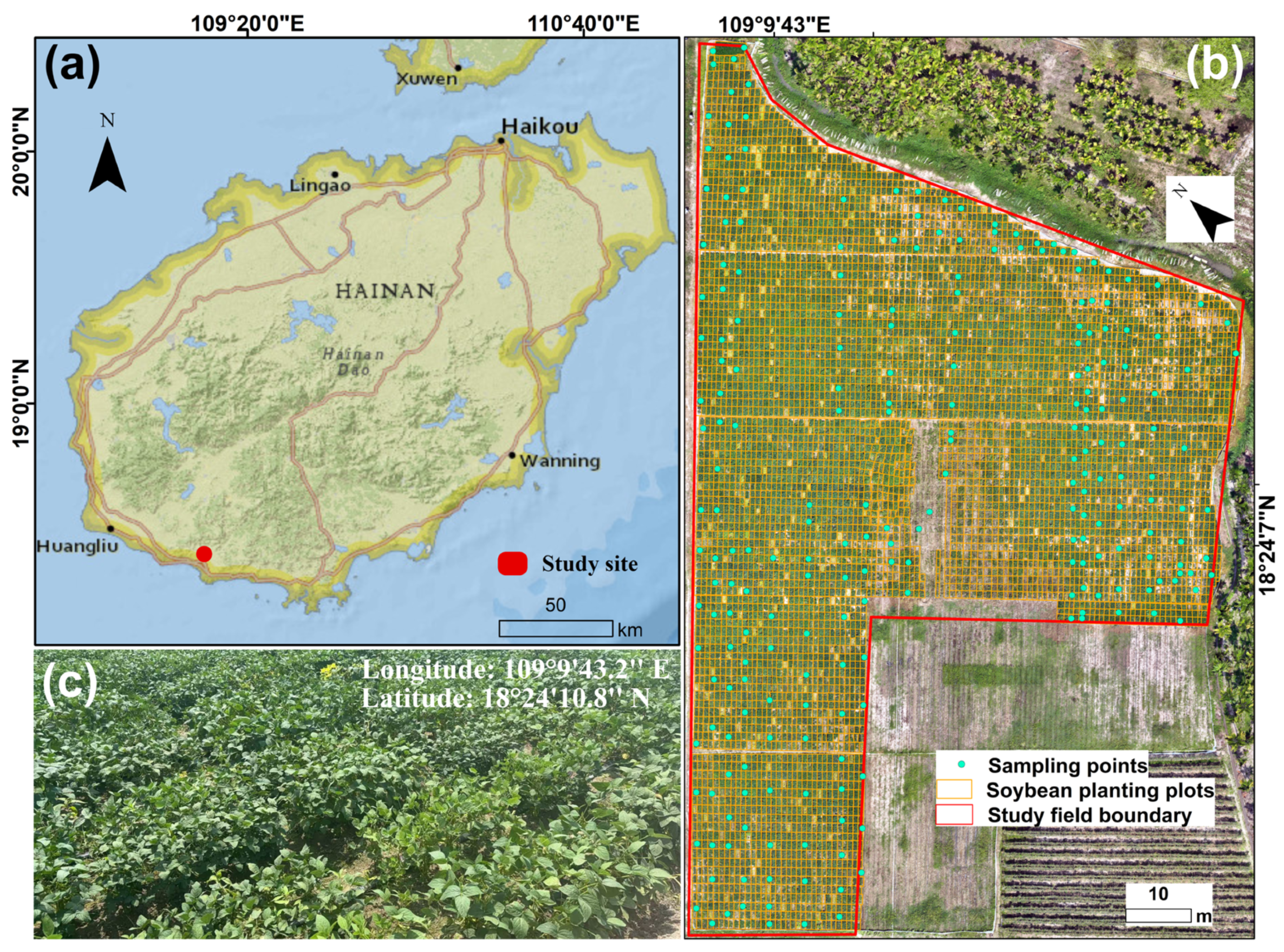
The field experiment was conducted in Chicao Village, Yazhou District, Sanya City, Hainan Province, China (Figure 1a). The experimental field is located at approximately 109°9′39.066″E to 109°9′45.587″E and 18°24′5″N to 18°24′10″N. The area has a tropical monsoon climate, with an average annual temperature of approximately 25.4 °C. The mean elevation is approximately 101 m, and the terrain is generally flat.

The soybean planting area covered approximately 1.3 ha and contained 6197 densely arranged rectangular planting plots. Soybeans were planted in mid-January 2024. Each plot represented a distinct soybean accession, and no accession was repeated among plots. Each plot covered approximately 1.5 m² (1.0 m × 1.5 m), contained four planting rows, and had a row spacing of 0.20 m and an approximate within-row plant spacing of 0.15 m. The nominal planting density was approximately 27 plants m⁻², and adjacent plots were separated by approximately 0.30 m.

The field was established as a large soybean germplasm screening panel rather than as a replicated randomized-block experiment because each accession was represented by a single planting plot. All plots received uniform and adequate irrigation and fertilization throughout the growing period. The exact irrigation volumes, fertilizer application rates and application dates were not retained in the field records.

A UAV RGB orthomosaic was used together with manually delineated plot polygons to define the field layout (Figure 1b). The final plot layer contained 6197 soybean planting plots. A total of 234 plots were selected by simple random sampling from the complete set of 6197 planting plots for paired SPAD and plant height measurements. Each measured plot represented a distinct soybean accession. These 234 plots were used for model development and validation, whereas the complete set of 6197 plot polygons was used only for subsequent field-scale prediction and mapping. A field photograph is provided to illustrate the canopy condition at the experimental site (Figure 1c).

2.2. Field Measurements of SPAD and PH

SPAD and PH were measured at the plot level on 15 March 2024 during the UAV survey period and served as the two reference traits for model development and validation. Paired measurements were obtained from 234 randomly selected plots, each representing a distinct soybean accession. SPAD was measured using a SPAD-502 chlorophyll meter (Konica Minolta Sensing, Inc., Osaka, Japan), following the standard instrument calibration and zeroing procedure. Within each plot, five plants were randomly selected and three fully expanded leaves were measured on each plant. Three readings were taken from the middle portion of each leaf blade while avoiding the main vein and leaf margins. The three readings were first averaged to obtain one leaf-level value, and the resulting 15 leaf-level values were then averaged to derive the plot-level SPAD value. PH was measured on five healthy, upright plants per plot using a measuring ruler. PH was defined as the vertical distance from the soil surface at the stem base to the apical growing point of the main stem. No lodging was observed in the measured plots, and the five plant-level measurements were averaged to obtain the plot-level PH value.

Field records were checked for missing entries, transcription inconsistencies and physically implausible measurements before model analysis. Measurements were not excluded solely because they were statistically extreme when no instrument or field-record error was identified, and all 234 plots retained complete paired SPAD and PH measurements. Observed SPAD values ranged from 8.30 to 85.90, with a mean of 43.01 and a standard deviation of 10.41, whereas PH ranged from 15.00 to 90.00 cm, with a mean of 43.89 cm and a standard deviation of 14.61 cm. The distributions of the measured SPAD and PH values are shown in Supplementary Figure S4. The broad observed ranges primarily reflected the biological diversity of the germplasm panel because the 234 measured plots represented 234 distinct accessions grown under common field management. This broad variation provided a useful calibration range, although observations were less densely represented at the distributional extremes, particularly at high SPAD values. The measured plots were linked to the manually delineated plot layer and subsequently combined with UAV-derived predictors for feature construction, model comparison and trait-specific evaluation.

2.3. UAV Data Acquisition and Preprocessing

UAV data were acquired using a DJI Mavic 3 Multispectral platform (SZ DJI Technology Co., Ltd., Shenzhen, China) equipped with one 20 megapixel RGB camera and four 5 megapixel multispectral cameras. The multispectral cameras captured Green (560 ± 16 nm), Red (650 ± 16 nm), RedEdge (730 ± 16 nm) and NIR (860 ± 26 nm) bands. The platform was equipped with an RTK module with nominal positioning precision of approximately 1 cm horizontally and 1.5 cm vertically. Because independent ground control points or checkpoints were not collected, these values should not be interpreted as independently verified horizontal or vertical accuracies of the final orthomosaic and DSM products. The interval from 11:00 to 14:00 on 15 March 2024 represented the overall field survey acquisition window rather than a single continuous three-hour flight. Imagery was acquired under cloud free conditions and wind speeds below 5 m·s⁻¹. Nadir imagery was collected at a flight altitude of 30 m, with forward and side overlaps both set to approximately 85%. The native ground sampling distances were approximately 0.8 cm·pixel⁻¹. for the RGB orthomosaic and 1.4 cm·pixel⁻¹ for the multispectral orthomosaics. Plot-level features were extracted from the respective products at their native resolutions without resampling to a common pixel size. Exact mission level records for flight duration, number of missions, image count, battery use, flight speed, flight line orientation, solar elevation, exposure and white balance were not retained and could not be reliably reconstructed.

UAV image processing was performed using Agisoft Metashape Professional version 1.8.5 (Agisoft LLC, St. Petersburg, Russia). RGB imagery was aligned and used for dense point cloud generation at an ultra-high-quality setting. The resulting DSM had a spatial resolution of approximately 1 cm. The DSM represented the visible canopy surface reconstructed from photogrammetry. Because reliable ground-point separation within the dense soybean canopy was limited, the DSM was used directly as a canopy surface product rather than interpreted as a fully ground-normalized canopy height model. Multispectral imagery acquired at the same flight altitude was processed to generate calibrated orthomosaics for the Green, Red, RedEdge and NIR bands. Raw digital numbers were converted to surface reflectance using images of diffuse reflectance panels with known reflectance acquired immediately before the flight. Optical and illumination variation was corrected using downwelling irradiance data recorded by the integrated sunshine sensor. Because acquisition occurred over the broader 11:00–14:00 survey window, some residual illumination variation may nevertheless remain, particularly in the RGB products. Plot boundaries were manually delineated in ArcGIS 10.7 and used as regions of interest for all plot-level feature extraction. These polygons excluded non-experimental buffer zones and defined the spatial unit for feature construction, model training, validation and field-scale prediction. The plot polygons were visually checked against the planting row boundaries before feature extraction. No internal polygon buffer or independently validated canopy mask was applied; all valid pixels within each manually delineated plot polygon were used for feature extraction.

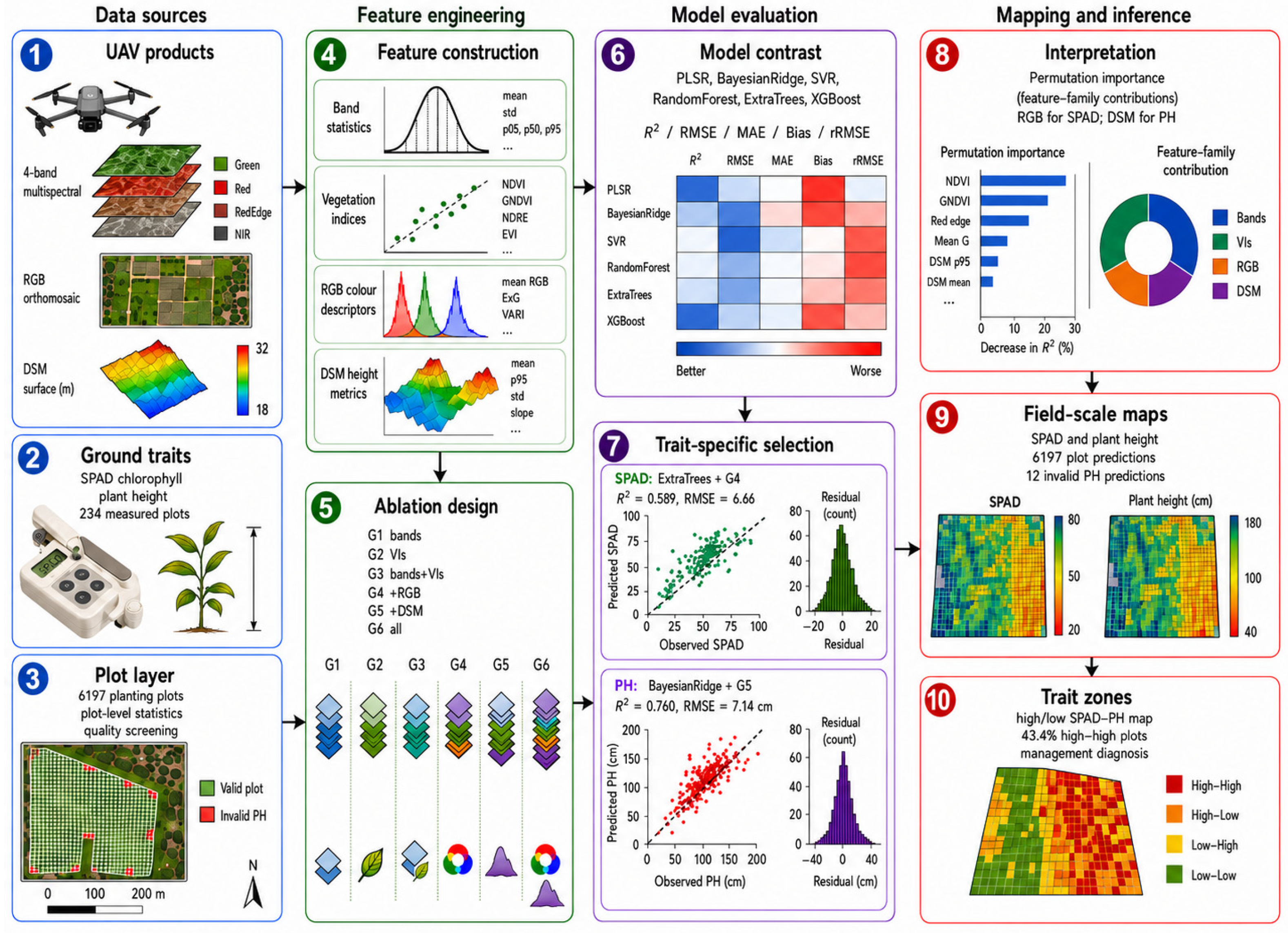
The workflow is shown in Figure 2. Field measurements, plot polygons and UAV products were combined to extract plot-level multispectral, RGB and DSM predictors. These predictors were organized into six feature groups and evaluated with six regression algorithms using random, spatial block and nested spatial cross-validation. One combination was retained for each trait and refitted using all 234 measured plots. The refitted models were then applied to the 6197 planting plots, followed by permutation importance analysis and field relative SPAD–PH classification.

2.4. Plot-Level UAV Feature Extraction and Feature Group Design

All UAV predictors were extracted within the manually delineated planting polygons. “Multispectral bands” refers to the calibrated Green, Red, RedEdge and NIR reflectance data. Nine plot-level statistics were calculated for each band. Vegetation indices were derived from these bands to represent transformed information related to canopy greenness, red-edge response and vegetation condition. RGB channel statistics and colour indices were extracted from the RGB orthomosaic to describe visible greenness, colour balance and canopy background contrast. Before calculating the RGB descriptors, the native channel values were rescaled to 0–1. This was a numerical rescaling and not a normalization by R + G + B. No additional radiometric or illumination correction was applied to the RGB data.

DSM features described the photogrammetrically reconstructed surface within each plot. They included mean, median, standard deviation, minimum, maximum, selected percentiles, range, coefficient of variation and percentile differences. The absolute statistics represent the reconstructed surface elevation and the dispersion and percentile-difference metrics describe within-plot surface variation. Because no ground-normalized terrain model was available, these variables were used as canopy surface descriptors and not as direct measurements of PH.

Nine statistics were calculated for each of the four multispectral bands, 16 vegetation indices and 10 RGB descriptors, producing 36 band predictors, 144 VI predictors and 90 RGB predictors. The DSM family contained 19 predictors. G1–G6 therefore contained 36, 144, 180, 270, 199 and 289 candidate predictors, respectively. Based on the 234 measured plots, the corresponding sample-to-predictor ratios were 6.50, 1.63, 1.30, 0.87, 1.18 and 0.81. Supplementary Table S1 provides the names, formulas, units and definitions of all indices and DSM metrics.

To evaluate the contribution of different UAV information sources, six feature groups were designed for ablation analysis (

Table 1. UAV feature groups used for ablation analysis. Predictor counts represent the candidate variables in each predefined feature group. The sample-to-predictor ratio was calculated using n = 234. During spatial-block and nested spatial cross-validation, the stated missingness and variation filters were reapplied within each training subset, so the number of predictors entering an individual fold could be slightly smaller.

Group	Feature Group	No. of Predictors	Sample-to-Predictor Ratio (n/p)	Main Information Represented
G1	Multispectral bands	36	6.50	Original Green, Red, RedEdge and NIR reflectance
G2	VIs	144	1.63	Transformed spectral information related to canopy greenness, chlorophyll sensitivity and vegetation condition
G3	Bands + VIs	180	1.30	Combination of original and transformed spectral predictors
G4	Bands + VIs + RGB descriptors	270	0.87	Spectral information plus visible greenness, colour balance and canopy background contrast
G5	Bands + VIs + DSM metrics	199	1.18	Spectral information plus reconstructed canopy surface elevation and within-plot surface variability
G6	Bands + VIs + RGB descriptors + DSM metrics	289	0.81	Full multisource UAV feature stack

VIs, vegetation indices; RGB, red–green–blue; DSM, digital surface model; UAV, unmanned aerial vehicle; NIR, near-infrared; RedEdge, red-edge spectral band; n, number of measured plots; p, number of candidate predictors.

). G1 served as the baseline spectral group, using only the original multispectral bands. G2 tested the contribution of vegetation index transformations. G3 evaluated the complementarity between original bands and vegetation indices. G4 added RGB descriptors to examine whether visible greenness and colour heterogeneity improved SPAD prediction. G5 added DSM-derived metrics to examine whether canopy surface structure improved PH prediction. G6 combined all feature groups and tested whether full multisource stacking outperformed the trait-specific feature combinations.

2.5. Model Training and Comparison

SPAD and PH were modelled separately because they represent distinct chlorophyll-related and structural dimensions of soybean canopy status. Six regression algorithms were compared, including partial least squares regression (PLSR) [29], BayesianRidge [30], support vector regression (SVR) [31], RandomForest [32], ExtraTrees [33] and XGBoost [34]. For each trait, all algorithms were evaluated under the six feature group settings described in Table 1, resulting in 36 algorithm–feature-group combinations. Table 1 reports the predictor counts after the initial quality screening and before the additional fold-specific screening used in the spatial validation analyses. All modelling and statistical analyses were implemented in Python 3.10.13 using NumPy 1.26.4, pandas 2.2.2, scikit-learn 1.4.2, XGBoost 2.0.3, SciPy 1.13.1, Matplotlib 3.8.4, and joblib 1.4.2. The complete software environment, preprocessing procedures, fixed model settings, and validation configuration are reported in Supplementary Table S2. PLSR used up to 10 latent components, with the actual number defined as a minimum of 10, the number of available predictors and the number of training observations minus one. BayesianRidge used the fixed parameter settings reported in Supplementary Table S2, corresponding to the defaults of scikit-learn version 1.4.2 unless otherwise specified. SVR used a radial-basis-function kernel with C = 10.0, gamma = “scale” and epsilon = 0.1. RandomForest and ExtraTrees each used 500 trees, square-root predictor subsampling, a minimum leaf size of two observations and random_state = 42. XGBoost used 500 trees, a maximum tree depth of three, a learning rate of 0.03, subsample and column-subsample fractions of 0.85, an L2 regularization parameter of 1.0, the squared-error regression objective and random_state = 42. All other parameters retained the defaults of the reported software versions. Hyperparameters were fixed before validation, and no grid search, random search, Bayesian optimization or other data-driven hyperparameter-tuning procedure was conducted.

Candidate predictors were screened according to data quality. Non-finite or non-convertible values were treated as missing and predictors with more than 35% missing values or no effective variation, defined as no more than one unique non-missing value, were excluded. No pairwise-correlation threshold or response-based variable-selection procedure was applied because G1–G6 were predefined as complete UAV information-source blocks. For random, spatial block and nested spatial cross-validation, the predictor quality screening criteria were applied within each corresponding training subset. Remaining missing values were imputed using medians estimated from the training observations and then applied unchanged to the held-out observations. StandardScaler was fitted using the training data for PLSR, BayesianRidge and SVR, whereas RandomForest, ExtraTrees and XGBoost used median imputation without standardization. Random cross-validation used shuffled fivefold KFold partitions with random_state = 42. For spatial block cross-validation, the plot centroid coordinates were centred and projected onto their principal spatial axis using singular value decomposition. Plots were ordered along this axis and divided into five adjacent blocks containing approximately equal numbers of measured plots. No spatial buffer was applied. In each iteration, one complete block was withheld for evaluation and the remaining four blocks were used for model fitting. The same fold assignments were used across all algorithms and feature groups.

To separate algorithm and feature-group selection from final performance evaluation, nested spatial cross-validation was additionally conducted. The five spatial blocks were used as outer validation folds. In each outer iteration, one block was withheld exclusively for evaluation while the remaining four blocks formed the outer-training dataset. Within the outer-training dataset, leave-one-spatial-block-out inner cross-validation was used to compare all 36 algorithm–feature-group combinations. The combination with the lowest pooled inner-cross-validated RMSE was selected, refitted using the complete outer-training dataset and evaluated on the untouched outer block. Ties were resolved using the higher inner-cross-validated R² followed by a fixed candidate order. Predictor screening, median imputation, feature scaling and model fitting were repeated using only the corresponding inner- or outer-training data. Model hyperparameters were specified before validation and were not optimized using either the inner or outer validation observations. All out-of-fold predictions were retained when calculating the cross-validation metrics. The physical quality control rule described in Section 2.7 was applied only to the final field-scale mapping outputs. Only the 234 plots with paired field measurements were used for model development and validation; the complete set of 6197 plots was used only for subsequent field-scale prediction. Because every planting plot represented a distinct soybean accession, genotype-grouped validation was not applicable.

Model performance was assessed using the coefficient of determination (R²), root mean square error (RMSE), mean absolute error (MAE), bias and relative RMSE (rRMSE). RMSE and MAE were reported in the original trait units, namely SPAD units for SPAD and centimetres for PH. Bias was calculated as the mean difference between predicted and observed values. Relative RMSE was calculated as RMSE divided by the observed trait mean and expressed as a percentage. Random and non-nested spatial cross-validation were used to describe comparative performance patterns among the 36 candidate combinations, whereas pooled outer-fold predictions from nested spatial cross-validation were used as the more conservative evaluation of the complete model-selection procedure. Selection stability was summarized separately for feature groups and complete algorithm–feature-group combinations. For field-scale mapping, the complete combination with the highest outer-fold selection frequency was retained. When two or more combinations shared the highest selection frequency, the tie was resolved by selecting the combination with the lowest mean inner-cross-validated RMSE across the five outer-training datasets. Models fitted using all measured plots were used only to generate field-scale predictions and were not treated as independent validation results.

2.6. Evaluating the Predictive Value of Feature Families

The block-level predictive value of the predefined feature families was evaluated using the G1–G6 ablation design. For each trait, the retained regression algorithm was held fixed across the six feature groups: ExtraTrees was used for SPAD and BayesianRidge for PH. Comparisons among G1, G2 and G3 examined the predictive value of transformed spectral information relative to the original multispectral bands. The comparison from G3 to G4 evaluated the incremental predictive value of RGB descriptors, whereas the comparison from G3 to G5 evaluated the incremental predictive value of DSM-derived structural metrics. G6 was used to determine whether the complete multisource feature stack improved prediction beyond the trait-specific combinations. Because G1–G6 contained different numbers of predictors, the ablation analysis was interpreted as a comparison of predefined information-source blocks under the same samples, validation partitions and modelling workflow, rather than as a dimension-matched or causal decomposition of biological effects. Differences among groups may therefore reflect the information represented by an added feature family together with predictor dimensionality, redundancy and interactions with model structure.

For the retained SPAD and PH mapping models, permutation importance was calculated after refitting each model using all 234 measured plots and the same preprocessing procedures and fixed hyperparameters described in Section 2.5. Each predictor was independently shuffled 30 times while all remaining predictors were left unchanged, using R² as the scoring metric and random_state = 42. Predictor importance was expressed as the mean decrease in R² across the 30 permutations, and the corresponding standard deviation was used to describe variability. Because predictors derived from the same UAV products can be strongly correlated, permutation importance may be shared or redistributed among related variables. These values were therefore used only for descriptive interpretation and were not treated as independent validation estimates. Individual predictor rankings were interpreted jointly with the feature-group ablation results and nested outer-fold selection frequencies, with emphasis placed on the broader predictive roles of spectral, RGB and structural information blocks rather than on the unique or causal effect of an individual predictor.

2.7. Field-Scale Prediction and Relative SPAD–PH Classification

After nested spatial evaluation, one mapping combination was retained for each trait and refitted using all 234 measured plots before application to the complete set of 6197 soybean planting plots. For SPAD, G4 was selected in four of the five outer folds, although the selected algorithm varied among PLSR, ExtraTrees, SVR and BayesianRidge. All five selected SPAD combinations were tied at one outer-fold selection; ExtraTrees with G4 was retained for field-scale mapping because it produced the lowest mean inner-cross-validated RMSE among these tied candidate combinations across the five outer-training datasets. For PH, G5 was selected in all five outer folds, with BayesianRidge selected in three folds and PLSR in two folds. BayesianRidge with G5 was therefore retained for PH mapping. These combinations are referred to as retained mapping models rather than as uniquely superior algorithms. Raw predictions were retained for traceability. Quality-controlled predictions were used for field-scale mapping and relative SPAD–PH classification.

Prediction quality control was conducted before generating the relative SPAD–PH classification map. SPAD predictions were retained because no physically invalid final SPAD values were produced. Predicted PH values of 0 cm or lower were considered physically invalid, retained as a separate quality control category and excluded from the four relative SPAD–PH classes.

Predicted SPAD and valid predicted PH were standardized into z-scores using the field-wide mean and standard deviation of each predicted trait. Plots were then assigned to four relative SPAD–PH classes according to the signs of the two z-scores: High SPAD–High PH, High SPAD–Low PH, Low SPAD–High PH and Low SPAD–Low PH. In this classification, “High” and “Low” indicate predicted values above and below the corresponding field-wide mean, respectively. The classes therefore describe relative combinations of predicted SPAD and PH within this experimental field and do not represent independent physiological, stress or agronomic thresholds. To characterize the joint distribution underlying the relative classification, Pearson’s correlation coefficient was calculated separately for the 234 paired field observations and for the quality-controlled field-scale SPAD and PH predictions. The predicted-data analysis excluded plots with physically invalid PH predictions. The corresponding observed and predicted joint distributions were examined using scatterplots, with the mean SPAD and PH values of each dataset shown as reference lines. These correlations were treated as descriptive summaries of the two datasets rather than as independent evidence of biological coupling between the traits. The final products included predicted SPAD, predicted PH and the four relative SPAD–PH classes for all valid plots, with invalid PH predictions retained as a separate quality control category.

3. Results

3.1. Model Performance and Algorithm Comparison

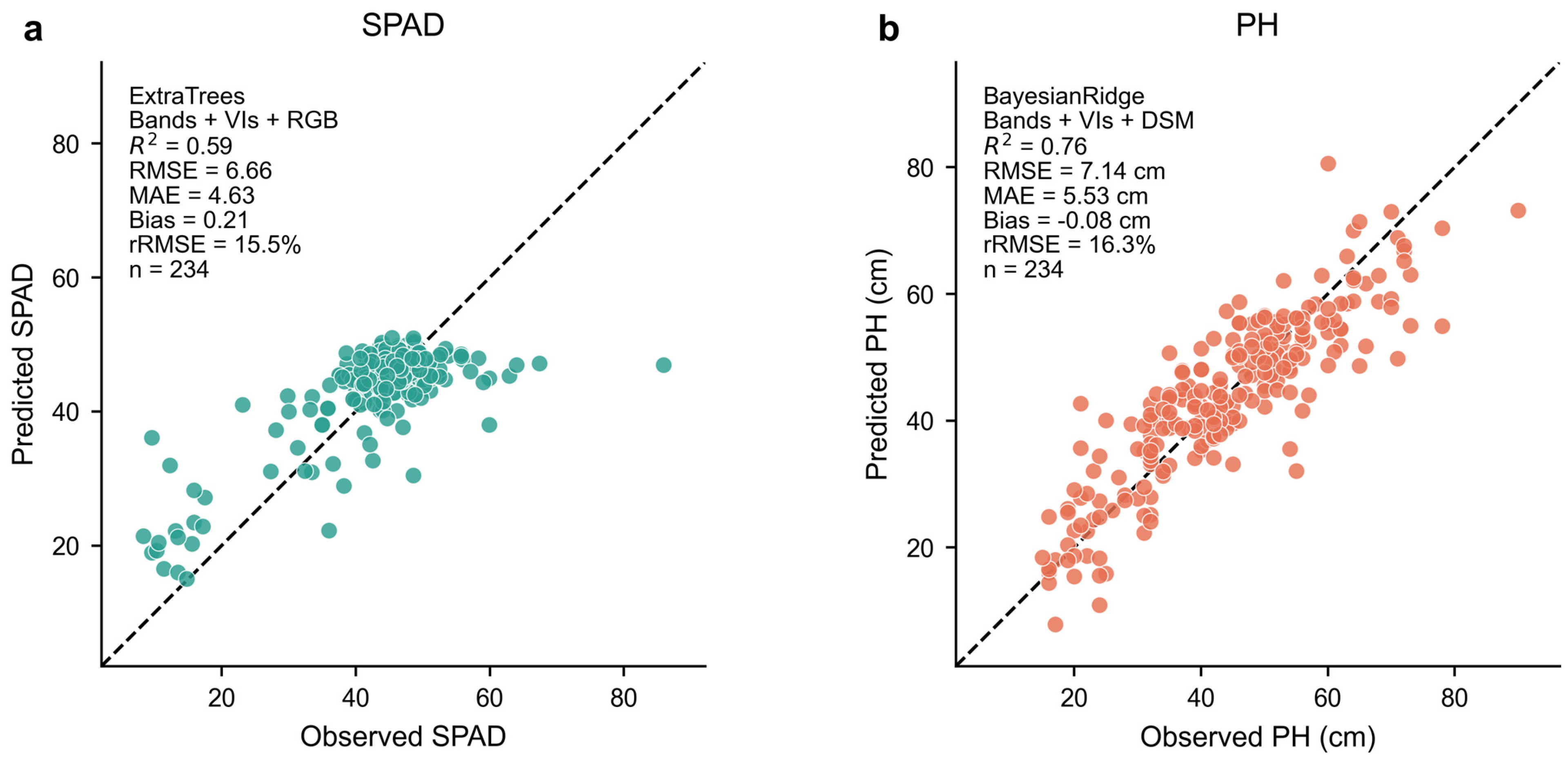
The random fivefold cross-validation comparison showed different performance patterns for SPAD and PH and identified the combinations subsequently retained for field-scale mapping (Figure 3). For SPAD, ExtraTrees with the G4 feature group, which combined multispectral bands, VIs, and RGB descriptors, produced the numerically highest R² and lowest RMSE under random cross-validation. This model achieved a cross-validated R² of 0.59, an RMSE of 6.66, an MAE of 4.63, a bias of 0.21 and an rRMSE of 15.5% (Figure 3a). The observed versus predicted relationship showed that predictions were concentrated around the central SPAD range and compressed at the upper end of the observed range. This pattern indicates that the model is more suitable for characterizing relative SPAD variation among plots than for accurately reproducing extreme high SPAD values.

For PH, BayesianRidge with the G5 feature group, which combined multispectral bands, VIs, and DSM-derived metrics, produced the numerically highest R² and lowest RMSE under random cross-validation. This model produced a cross-validated R² of 0.760, an RMSE of 7.14 cm, an MAE of 5.53 cm, a bias of −0.08 cm, and an rRMSE of 16.3% (Figure 3b). Compared with SPAD, PH showed a tighter observed versus predicted relationship.

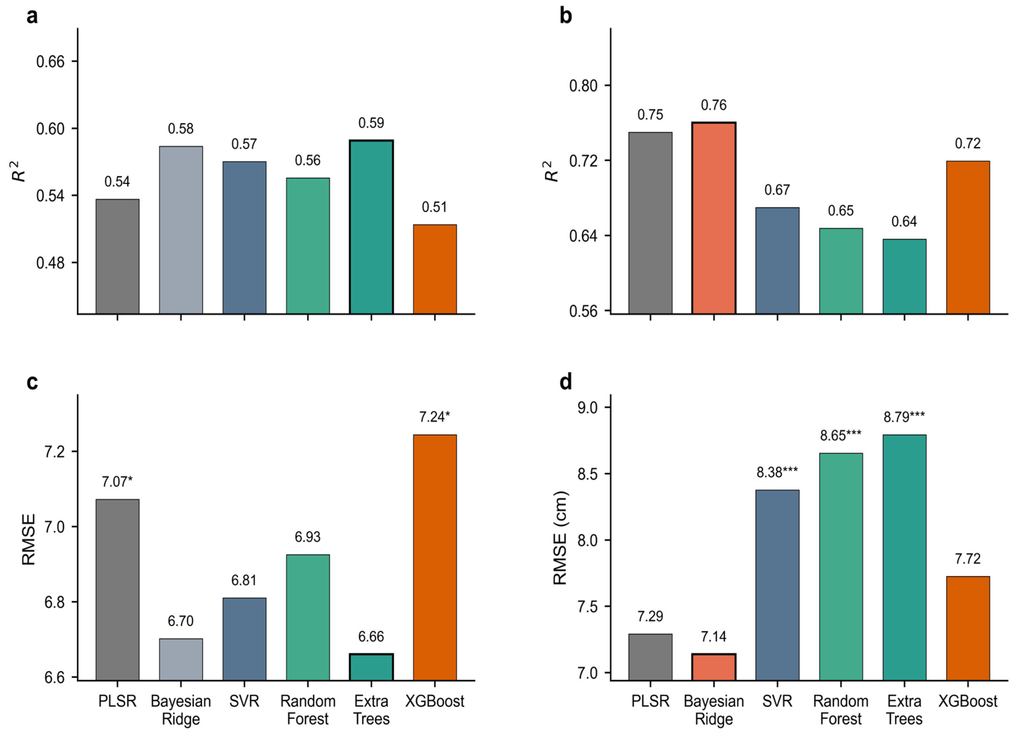
The algorithm comparison under the selected feature settings showed that model ranking differed between the two traits (Figure 4). For SPAD under the G4 setting, ExtraTrees achieved the lowest RMSE, followed by BayesianRidge, SVR, RandomForest, PLSR and XGBoost. Paired tests based on cross-validated absolute errors showed that PLSR and XGBoost had significantly higher errors than ExtraTrees after Holm correction. The differences between ExtraTrees and BayesianRidge, SVR and RandomForest were not significant (Figure 4c).

For PH under the G5 setting, BayesianRidge achieved the lowest RMSE, followed by PLSR, XGBoost, SVR, RandomForest and ExtraTrees. SVR, RandomForest and ExtraTrees had significantly higher errors than BayesianRidge after Holm correction (Figure 4d). PLSR and XGBoost showed lower errors than the other non-selected models, but their differences from BayesianRidge were not significant after correction.

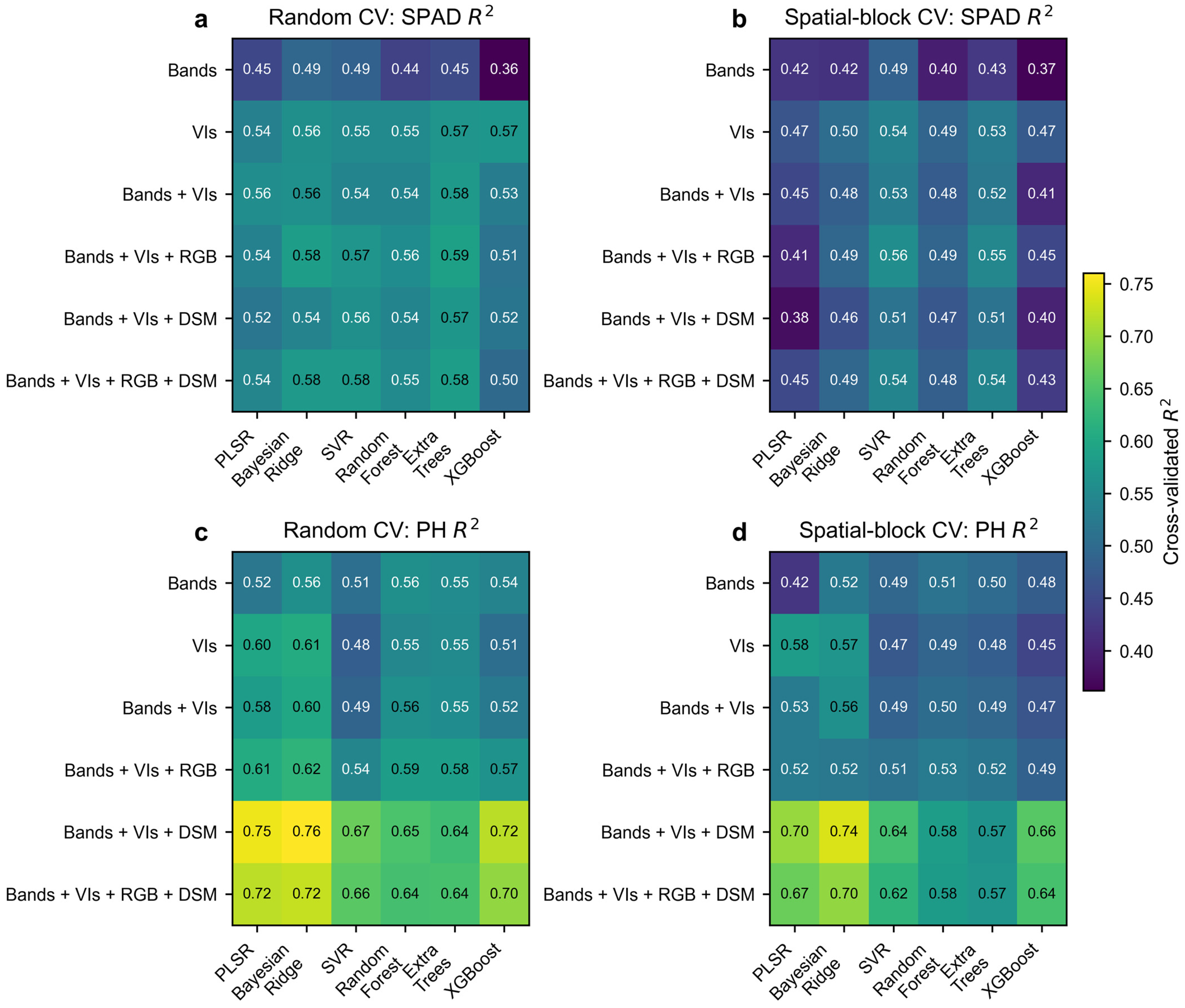
The complete performance matrices further showed how the feature-group patterns changed between random and spatially blocked cross-validation (Figure 5). Under random cross-validation, ExtraTrees with G4 produced the numerically highest SPAD performance (R² = 0.59), whereas BayesianRidge with G5 produced the highest PH performance (R² = 0.76). Under spatial block cross-validation, the corresponding selected combinations retained similar performance, with R² = 0.546 and RMSE = 7.00 for SPAD and R² = 0.737 and RMSE = 7.49 cm for PH.

For SPAD, the precise algorithm ranking changed slightly under spatial blocking. SVR with G4 produced the numerically highest spatially blocked R² of 0.56, while ExtraTrees with G4 remained nearly equivalent at R² = 0.55. Across the six algorithms, G4 generally remained competitive, but the addition of RGB descriptors did not improve every model. These results indicate that RGB descriptors provided a small and model-dependent incremental contribution rather than a uniformly strong improvement in SPAD prediction.

The PH pattern was more consistent across the two validation strategies. Feature groups containing DSM metrics, particularly G5, clearly outperformed groups based only on bands, VIs or RGB descriptors. Under spatial block cross-validation, BayesianRidge with G5 retained the highest R² of approximately 0.74, followed by PLSR with G5 at 0.70. Adding RGB descriptors to form the complete G6 stack did not further improve PH performance. Thus, spatial separation produced only modest reductions in accuracy and did not alter the principal conclusion that DSM-derived information contributed more clearly to PH than RGB descriptors contributed to SPAD.

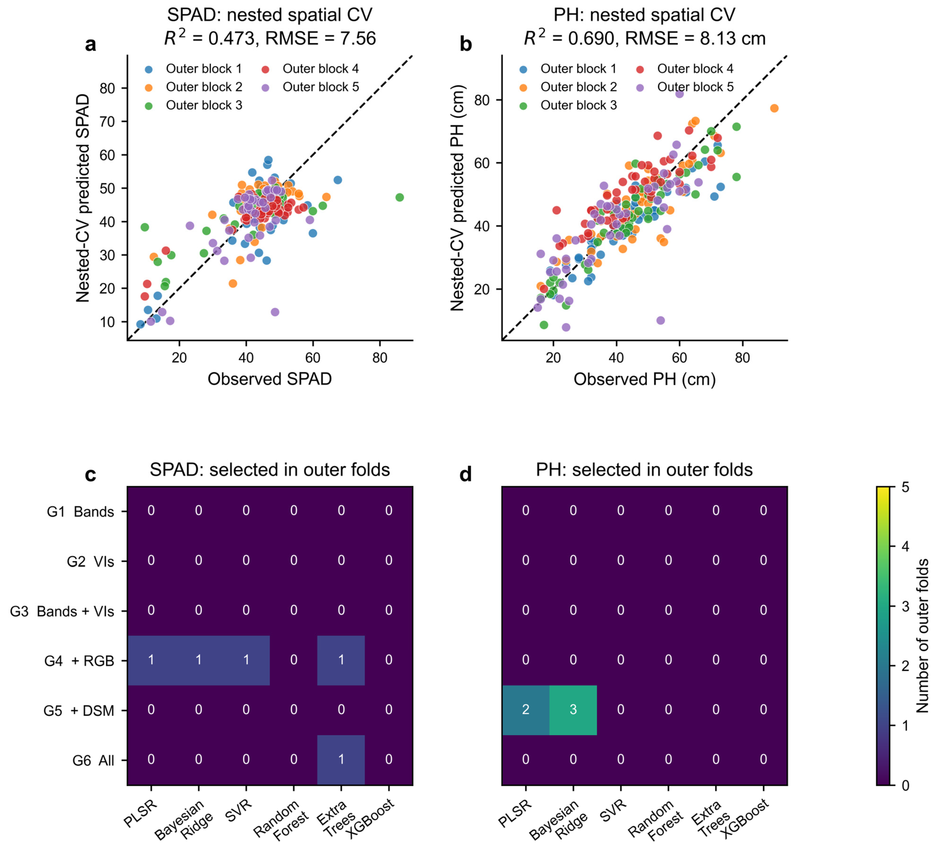
Nested spatial cross-validation provided a more conservative evaluation in which algorithm and feature-group selection was conducted entirely within the outer-training data (Figure 6). The pooled outer-fold predictions yielded R² = 0.473, RMSE = 7.56, and MAE = 5.24 for SPAD. For PH, the corresponding nested estimates were R² = 0.690, RMSE = 8.13 cm, and MAE = 6.11 cm.

For SPAD, G4 was selected in four of the five outer folds, but no single algorithm was consistently dominant. PLSR, ExtraTrees, SVR and BayesianRidge with G4 were each selected once, while the remaining fold selected ExtraTrees with G6. Thus, the G4 feature-family pattern was more stable than the identity of a specific SPAD algorithm. Because all five complete combinations were tied at one outer-fold selection, their mean inner-cross-validated performance across the five outer-training datasets was compared. ExtraTrees with G4 had the lowest mean inner-cross-validated RMSE of 7.18, followed closely by SVR with G4 at 7.20, and was therefore retained for field-scale mapping.

For PH, G5 was selected in all five outer folds. BayesianRidge with G5 was selected in three folds and PLSR with G5 in two folds. BayesianRidge with G5 also had a lower mean inner-cross-validated RMSE across the outer-training datasets than PLSR with G5 (8.37 versus 8.54 cm) and was therefore retained as the PH mapping combination. Overall, the nested results provided stronger evidence for the stability of the trait-specific feature groups—particularly G5 for PH—than for the universal superiority of an individual regression algorithm.

3.2. Feature-Group Contribution and Important Predictors

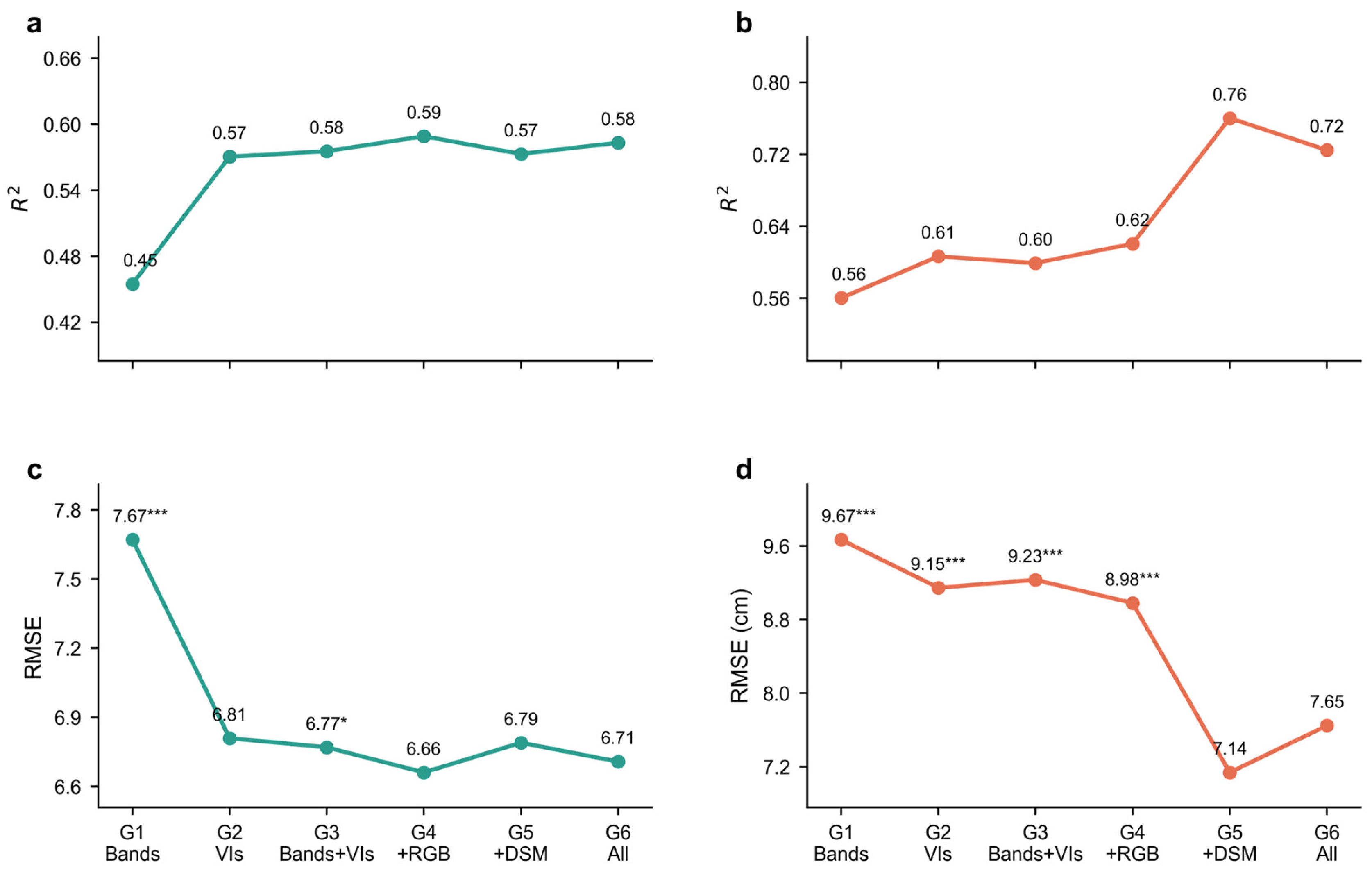
The feature-group ablation analysis showed a trait-dependent pattern in the contribution of UAV information sources (Figure 7). For SPAD, the bands-only baseline produced an R² of 0.46 and an RMSE of 7.67. VIs improved performance to R² = 0.57 and RMSE = 6.81. Combining multispectral bands with vegetation indices produced a similar result (R² = 0.58, RMSE = 6.77). Under random cross-validation, the numerically highest SPAD performance was obtained after adding RGB descriptors in G4, with R² increasing to 0.59 and RMSE decreasing to 6.66. Adding DSM metrics in G5 did not improve performance beyond G4, and the full feature stack in G6 was slightly weaker than G4. Paired tests showed that G1 and G3 had significantly higher absolute errors than G4 after Holm correction (Figure 7c).

For PH, the bands-only baseline produced an R² of 0.56 and an RMSE of 9.67 cm. VIs improved performance to R² = 0.61 and RMSE = 9.15 cm; G3 showed similar performance (R² = 0.60, RMSE = 9.23 cm). Adding RGB descriptors in G4 resulted in a limited gain (R² = 0.62, RMSE = 8.98 cm). Under random cross-validation, the largest improvement occurred when DSM metrics were added in G5, which increased R² to 0.76 and reduced RMSE to 7.14 cm. Performance declined again when all feature groups were combined in G6. Paired tests showed that G1, G2, G3 and G4 had significantly higher absolute errors than G5 after Holm correction (Figure 7d). Model performance did not increase monotonically with predictor number. G6 contained the largest candidate feature set, with 298 predictors, but did not outperform G4 for SPAD or G5 for PH. Thus, the observed rankings cannot be explained simply by the inclusion of more variables. Nevertheless, because the feature groups were not matched in dimensionality, their performance differences are interpreted as block-level predictive comparisons rather than as a dimension-controlled decomposition of biological effects. The nested spatial analysis provided an additional assessment of feature-group stability: G4 was selected in four of the five outer folds for SPAD, whereas G5 was selected in all five outer folds for PH.

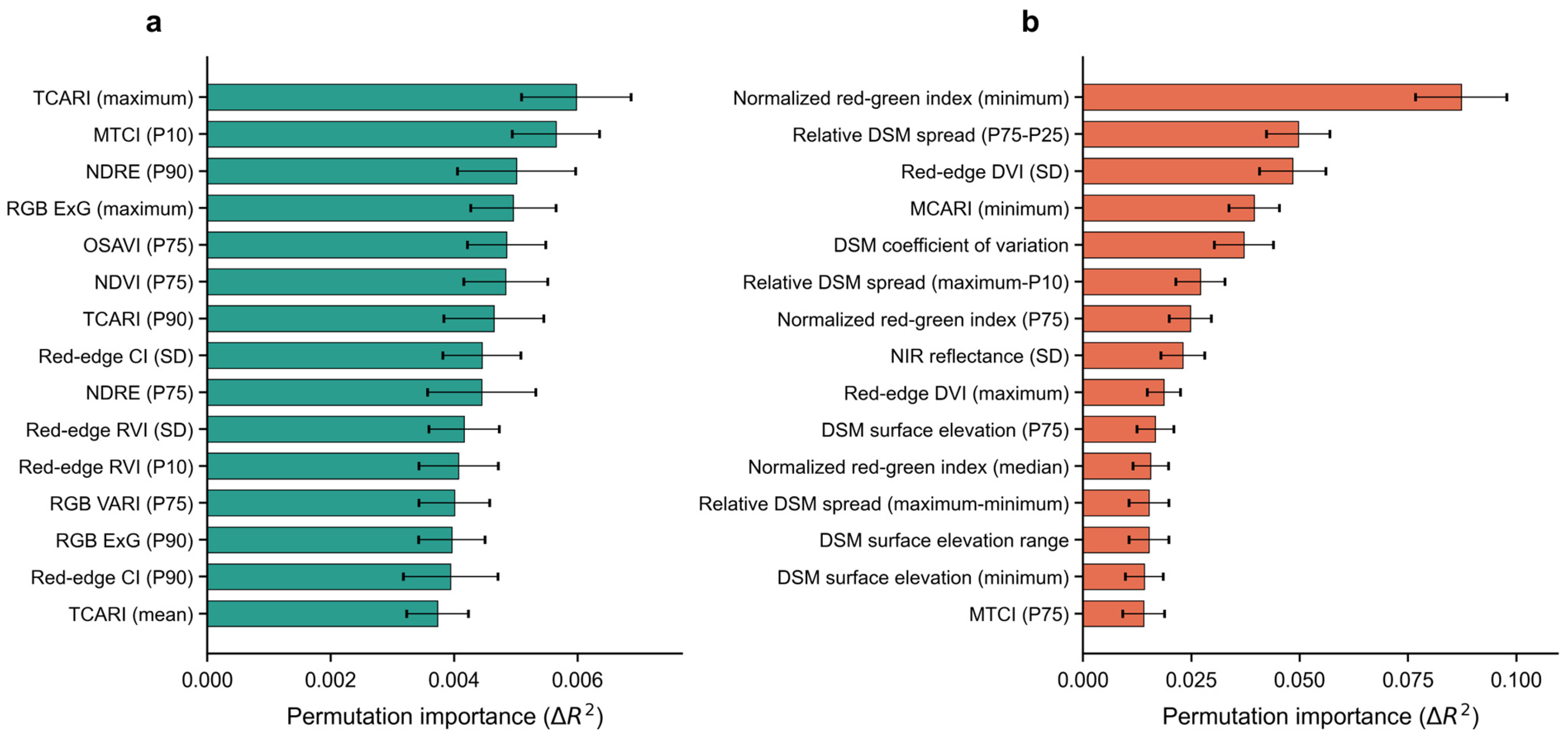
Permutation importance further identified the dominant predictors within the selected models (Figure 8). For SPAD, the highest ranked predictors included TCARI max, MTCI p10, NDRE p90, RGB ExG max, OSAVI p75, NDVI p75 and TCARI p90 (Figure 8a). For PH, the top-ranked predictors included the minimum normalized red–green index, the relative DSM percentile spread (P75–P25), the standard deviation of the red-edge DVI, the minimum MCARI, the DSM coefficient of variation, the relative DSM upper spread (maximum–P10), and the P75 of the normalized red–green index (Figure 8b). These rankings were interpreted descriptively because correlated predictors may share or redistribute permutation importance. Among the leading variables, the retained SPAD model contained several vegetation-index and RGB predictors. The retained PH model included several DSM-derived and within-plot structural variability predictors.

3.3. Field-Scale Prediction Results and Relative SPAD–PH Patterns

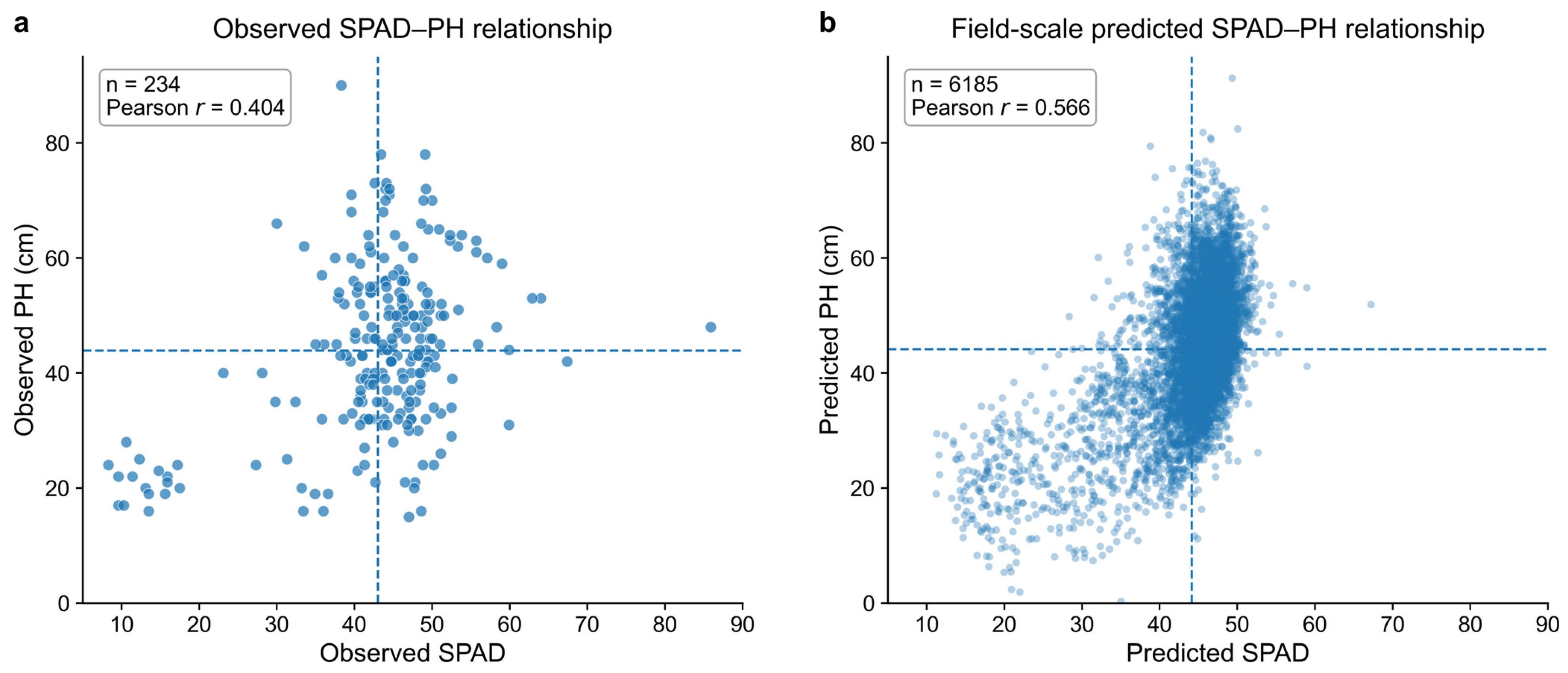
The paired field observations showed a moderate positive association between SPAD and PH (Pearson’s r = 0.404, n = 234; Figure 9a). After excluding the 12 plots with physically invalid PH predictions, the quality-controlled field-scale predictions showed a stronger positive association (r = 0.566, n = 6185; Figure 9b). The joint predicted distribution was therefore more strongly concentrated along a positive SPAD–PH gradient than the observed distribution. Consequently, the relative abundance of the four SPAD–PH classes should be interpreted in relation to both the marginal distributions and the positive association between the two predicted traits rather than as evidence of discrete biological types.

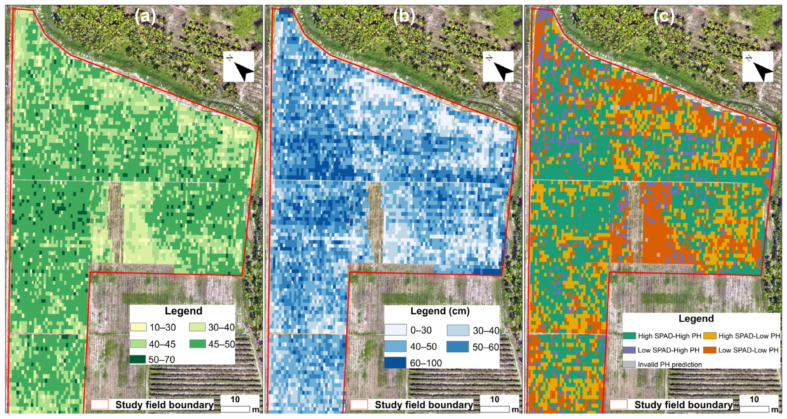
The final trait-specific models were applied to all 6197 soybean planting plots to generate field-scale prediction products (Figure 10). Predicted SPAD values ranged from 11.20 to 67.19 (Figure 10a), while quality-controlled PH predictions ranged from 0.32 to 91.26 cm (Figure 10b). Only 12 plots were flagged as invalid PH predictions, accounting for 0.19% of all plots. The SPAD and PH maps showed clear spatial heterogeneity across the field.

To compare relative within-field variation, predicted SPAD and valid predicted PH were standardized as z-scores. The corresponding z score maps are provided in Figure S3. These maps show the relative position of each plot within the field-wide prediction distribution, where negative values indicate below average predictions and positive values indicate above average predictions. The z score maps also provided the basis for the subsequent relative SPAD–PH classification.

After excluding the 12 plots with invalid PH predictions, 6185 plots remained for the relative SPAD–PH classification (Figure 10c). Among the valid plots, the High SPAD–High PH class contained 2689 plots (43.48%), the High SPAD–Low PH class contained 1529 plots (24.72%), the Low SPAD–High PH class contained 572 plots (9.25%), and the Low SPAD–Low PH class contained 1395 plots (22.55%). Invalid PH predictions were retained as a separate quality control category and were not included in the class percentages.

4. Discussion

4.1. Trait-Specific Feature Contribution and Model Interpretation

Previous UAV phenotyping studies have demonstrated the value of combining spectral, colour, texture and structural information for crop trait estimation, including soybean yield prediction, growth monitoring and canopy structure assessment [22,24,26,35]. However, multisource predictors are often evaluated as a single fused feature pool or for one target trait at a time, making it difficult to determine whether the same information source provides equal predictive value for chlorophyll-related and structural traits. The methodological contribution of the present study is therefore not a new regression algorithm but a controlled comparison of six predefined UAV information-source blocks using the same measured plots, validation partitions and model set. The groups nevertheless differed substantially in dimensionality, ranging from 36 predictors in G1 to 289 predictors in G6. Their performance differences should therefore not be interpreted as a dimension-controlled or causal decomposition of biological effects but as comparisons of complete information-source blocks that may reflect information content together with redundancy, dimensionality and model-specific regularization.

Performance did not increase monotonically with feature-group size. Vegetation indices provided a common predictive basis, RGB descriptors produced a small and model-dependent incremental gain for SPAD, and DSM-derived metrics produced the principal improvement in PH. The complete G6 stack contained the largest number of predictors but did not outperform G4 for SPAD or G5 for PH, indicating that predictor number alone did not determine the rankings. At the same time, because the groups were not matched in dimensionality, the differences cannot be attributed exclusively to the biological relevance of a feature source. These findings are therefore interpreted as block-level predictive patterns within the evaluated modelling framework.

Spatial-block and nested spatial cross-validation provided additional assessments of the stability of these patterns. For the retained combinations, spatial-block R² values were 0.546 for SPAD and 0.737 for PH, compared with random-cross-validation values of 0.589 and 0.760, respectively. Nested spatial cross-validation yielded more conservative estimates of R² = 0.473 for SPAD and R² = 0.690 for PH. G4 was selected in four of the five SPAD outer folds, although the selected algorithm varied among PLSR, ExtraTrees, SVR and BayesianRidge. In contrast, G5 was selected in all five PH outer folds, with BayesianRidge selected in three folds and PLSR in two. These results provide stronger evidence of the stability of the broad feature-family pattern—particularly the predictive value of DSM-containing features for PH—than for the universal superiority of an individual predictor or algorithm.

The moderate predictive performance, particularly for SPAD, likely resulted from limitations in the reference data and feature representation rather than from the choice of a single algorithm. The 234 measured plots represented a broad soybean panel, but observations were less densely represented at the extremes and all UAV predictors were derived from one acquisition date. SPAD was based on leaf measurements summarized to the plot level, whereas the UAV predictors represented the visible canopy surface, creating an observational-scale mismatch. PH corresponded more directly to the DSM-derived canopy surface metrics and therefore achieved higher accuracy, although these metrics should not be interpreted as direct ground-normalized PH. In addition, the large number of correlated predictors relative to the measured sample size may have limited model generalization and redistributed permutation importance among related variables. The similar performance of several algorithms suggests that the main constraints arose from the reference data and predictor representation rather than from model choice alone.

4.2. Interpretation of UAV Feature Responses for SPAD and PH

SPAD is widely used as an indicator of leaf chlorophyll-related status, but it is not equivalent to directly measured chlorophyll content. UAV imagery observes the visible canopy surface, whereas SPAD measurements are leaf-based observations aggregated to the plot level. Chlorophyll-sensitive indices such as NDRE, MTCI, MCARI and TCARI are useful because they respond to pigment absorption and red-edge reflectance patterns [10,11]. However, canopy level spectral responses are also affected by canopy structure, soil background, illumination and saturation [14,36]. Together, these factors help explain the moderate SPAD accuracy and the compression of predictions at the high end of the observed range. The model should therefore be interpreted primarily as a tool for characterizing relative plot-level SPAD variation; predictions at the extreme upper end should be treated with caution. The broad observed range was useful for model calibration because it included contrasting soybean phenotypes. However, the smaller number of observations at the extremes, particularly at high SPAD values, likely caused the predictions to regress toward the central range. The SPAD model should therefore be interpreted mainly as a tool for characterizing relative variation among plots rather than for precise prediction of extreme values. Because all algorithms and feature groups were evaluated using the same measured plots and validation partitions, the uneven trait distribution does not change the main comparative conclusions regarding trait-specific feature contributions, although it affects absolute prediction accuracy.

RGB descriptors should be interpreted as visible colour features rather than as a completely separate non-spectral data source. Although RGB information is also optical information, it differs from calibrated multispectral bands because it captures fine resolution visible greenness, colour balance and canopy background contrast. ExG and related colour descriptors have been widely used to describe green vegetation cover and separate vegetation from soil background [17,18]. In dense soybean plots, such visible colour descriptors can complement vegetation indices by representing canopy cover, row gaps and within-plot heterogeneity. Their contribution to SPAD prediction should therefore be understood as an indirect canopy colour signal rather than a direct chlorophyll measurement.

For PH, the contribution of DSM features is consistent with the structural nature of the trait. The DSM represented the visible canopy surface reconstructed from photogrammetry; its percentiles, dispersion measures and percentile differences described plot-level surface elevation and structural variability. Previous UAV studies have shown that photogrammetric crop-surface products can support high-throughput crop height estimation [19,20,31]. In the present relatively flat field, DSM dispersion and percentile-difference metrics were useful because they emphasized within-plot surface variation and were less affected by a common local elevation offset than absolute DSM values. However, the DSM metrics were not equivalent to direct PH measurements or to a fully ground-normalized canopy height model. Their strong contribution should therefore be interpreted as evidence that the reconstructed canopy surface structure improved PH prediction in this field. In fields with stronger microrelief, terrain normalization or point-cloud-based ground modelling would be required before transferring the same structural interpretation.

4.3. Field-Scale Interpretation of Relative SPAD–PH Classes

The joint SPAD–PH classification provides a simple way to summarize the relative positions of plots within the field-wide prediction distributions. The four classes were defined only by whether predicted SPAD and PH were above or below their corresponding field means. High SPAD–High PH and Low SPAD–Low PH therefore indicate plots in which the two predicted traits vary in the same relative direction, whereas High SPAD–Low PH and Low SPAD–High PH indicate contrasting relative patterns. These classes describe within-field combinations of predicted SPAD and PH rather than independently defined physiological states. The observed SPAD–PH relationship was moderately positive (r = 0.404), whereas the association between the two field-scale predictions was stronger (r = 0.566). This positive covariance contributed to the relatively large proportion of plots assigned to the High SPAD–High PH class. However, the predicted correlation may also reflect shared predictor information, model smoothing and the marginal distributions of the two model outputs. Consequently, neither the predicted correlation nor the class proportions demonstrate the existence of discrete biological classes. They provide only a relative summary of joint predicted SPAD and PH variation within this field and acquisition date.

The classification should not be interpreted as a direct mapping of crop stress, nutritional condition, yield potential or genotype superiority. Its thresholds depend on the predicted distributions in this particular field and may change in another field, growth stage or season. The main value of the classification is to support relative comparison and targeted follow-up sampling by identifying plots with similar or contrasting predicted SPAD and PH patterns. Independent measurements of yield, nutrient status or stress would be required before specific agronomic interpretations could be assigned to these classes.

4.4. Limitations and Future Perspectives

Several limitations should be noted. First, the models were developed using 234 measured plots from a single field experiment and UAV imagery acquired on one observation date, 15 March 2024. Spatial-block and nested spatial cross-validation were added to reduce the influence of local spatial similarity and to separate algorithm–feature-group selection from outer-fold evaluation. Nevertheless, all validation strategies remained internal to the same field, acquisition date, growth stage and management environment. The present results therefore demonstrate within-field robustness rather than transferability across environments or seasons. Because the soybean accessions were evaluated on the same calendar date but could differ in developmental stage, part of the observed variation in SPAD, PH, canopy cover and UAV-derived predictors may reflect phenological differences among accessions. The present single-date analysis could not separate these phenological effects from other accession-related differences. In addition, each soybean accession was represented by a single planting plot, so genotype-level biological replication was unavailable and accession-related variation could not be completely separated from localized environmental heterogeneity. Although all plots received uniform and adequate irrigation and fertilization, the exact irrigation volumes, fertilizer application rates and application dates were not retained in the field records. Independent validation using replicated experiments across additional years, sites and growth stages remains necessary before the retained feature-group patterns can be considered broadly transferable.

Second, the SPAD measurements and UAV predictors represented different observational scales. Although plot-level SPAD was averaged from measurements of 15 leaves across five plants, the original observations remained leaf-based whereas the UAV predictors summarized spectral and colour information across the complete plot polygons. The SPAD model should therefore be interpreted as predicting a plot-level average indirectly associated with canopy spectral response and visible colour, which may also reflect canopy cover, row gaps, shadows and background exposure. It does not provide a direct retrieval of leaf chlorophyll content. Because no internal polygon buffer or independently validated canopy mask was used, residual edge mixing, shadows, exposed soil and uncertainty in the manually delineated plot boundaries may also have affected some plot-level predictors. This scale mismatch, together with the absence of an independently validated canopy mask, may partly explain the reduced sensitivity at the extremes of the SPAD distribution. Future studies should compare whole-plot and canopy-mask-based feature extraction using independently validated vegetation masks and more spatially intensive leaf sampling.

Third, the PH analysis used DSM-derived canopy surface metrics rather than a fully ground-normalized canopy height model. Dense soybean cover limited reliable ground-point separation within the planting plots. Estimating the ground surface from surrounding bare areas would require the assumption of a nearly level field. The experimental field was relatively flat, so within-plot DSM dispersion and percentile-difference metrics remained useful for characterizing relative structural differences. Nevertheless, absolute DSM statistics may include residual effects of ground elevation, and the resulting predictions should not be interpreted as direct canopy-height retrievals. Constructing a valid ground-normalized canopy-height model would require an independent pre-emergence terrain survey or reliable ground observations within the planting plots; neither was available in the present experiment and neither can be reconstructed retrospectively from the densely closed canopy. Fourth, the field-scale maps were generated without a formal applicability domain or feature novelty assessment. Consequently, the study could not determine which predictions for the 5963 unmeasured plots represented interpolation within the calibration feature space and which represented multivariate extrapolation. Plot-specific calibrated prediction intervals were also unavailable. The maps should therefore be interpreted as exploratory within-field point predictions rather than applicability-screened or uncertainty-calibrated products.

5. Conclusions

This study showed that soybean SPAD and PH did not benefit from the same predefined UAV feature combination. Although vegetation indices formed a common predictive basis for both traits, the additional information required for improving model performance was clearly trait-specific. Under random fivefold cross-validation, ExtraTrees with G4 produced the numerically highest SPAD performance (R² = 0.589; RMSE = 6.66) but BayesianRidge with G5 produced the numerically highest PH performance (R² = 0.760; RMSE = 7.14 cm). When algorithm and feature-group selection were separated from final evaluation using nested spatial cross-validation, the corresponding outer-fold estimates decreased to R² = 0.473 and RMSE = 7.56 for SPAD and R² = 0.690 and RMSE = 8.13 cm for PH. G4 was selected in four of the five outer folds for SPAD, although no single SPAD algorithm was consistently dominant. In contrast, G5 was selected in all five outer folds for PH, providing stronger evidence for the stability of the DSM-containing feature group. ExtraTrees with G4 and BayesianRidge with G5 were retained as representative field-scale mapping combinations rather than as uniquely superior algorithms. RGB descriptors therefore provided only a small and model-dependent incremental contribution to SPAD, whereas DSM-derived canopy surface metrics provided a larger and more stable contribution to PH. These DSM-based predictors should be interpreted as canopy surface indicators rather than as direct ground-normalized canopy-height measurements. Importantly, the full feature stack was not optimal for either trait, demonstrating that UAV multisource fusion should not be treated as simple feature accumulation. Instead, feature selection should be guided by the biological interpretation of the target trait and supported by validation evidence. Applying the retained models to all 6197 soybean plots provided a within-field, single-date characterization of relative SPAD and PH variation and a basis for targeted follow-up sampling, rather than evidence of model transferability across years, sites or growth stages.

References

1. Alves, A.K.; Araújo, M.S.; Chaves, S.F.; Dias, L.A.S.; Corrêdo, L.P.; Pessoa, G.G.; Bezerra, A.R. High throughput phenotyping in soybean breeding using RGB image vegetation indices based on drone. Sci. Rep. 2024, 14, 32055. [Google Scholar] [CrossRef] [PubMed]
2. Araus, J.L.; Cairns, J.E. Field high-throughput phenotyping: The new crop breeding frontier. Trends Plant Sci. 2014, 19, 52–61. [Google Scholar] [PubMed]
3. Bendig, J.; Yu, K.; Aasen, H.; Bolten, A.; Bennertz, S.; Broscheit, J.; Gnyp, M.L.; Bareth, G. Combining UAV-based plant height from crop surface models, visible, and near infrared vegetation indices for biomass monitoring in barley. Int. J. Appl. Earth Obs. Geoinf. 2015, 39, 79–87. [Google Scholar] [CrossRef]
4. Berveglieri, A.; Imai, N.N.; Watanabe, F.S.Y.; Tommaselli, A.M.G.; Ederli, G.M.P.; de Araújo, F.F.; Lupatini, G.C.; Honkavaara, E. Remote prediction of soybean yield using UAV-Based Hyperspectral Imaging and Machine Learning models. AgriEngineering 2024, 6, 3242–3260. [Google Scholar] [CrossRef]
5. Broge, N.H.; Leblanc, E. Comparing prediction power and stability of broadband and hyperspectral vegetation indices for estimation of green leaf area index and canopy chlorophyll density. Remote Sens. Environ. 2001, 76, 156–172. [Google Scholar] [CrossRef]
6. Chen, T.; Guestrin, C. XGBoost: A Scalable Tree Boosting System. In Proceedings of the 22nd ACM SIGKDD International Conference on Knowledge Discovery and Data Mining. Presented at the KDD ’16: The 22nd ACM SIGKDD International Conference on Knowledge Discovery and Data Mining; ACM: San Francisco, CA, USA, 2016; pp. 785–794. [Google Scholar] [CrossRef]
7. Cortes, C.; Vapnik, V. Support-vector networks. Mach. Learn. 1995, 20, 273–297. [Google Scholar] [CrossRef]
8. Dash, J.; Curran, P.J. The MERIS Terrestrial Chlorophyll Index. Int. J. Remote Sens. 2004, 25, 5403–5413. [Google Scholar] [CrossRef]
9. Daughtry, C.S.; Walthall, C.L.; Kim, M.S.; De Colstoun, E.B.; McMurtrey, J.E., III. Estimating corn leaf chlorophyll concentration from leaf and canopy reflectance. Remote Sens. Environ. 2000, 74, 229–239. [Google Scholar] [CrossRef]
10. Fisher, A.; Rudin, C.; Dominici, F. All models are wrong, but many are useful: Learning a variable’s importance by studying an entire class of prediction models simultaneously. J. Mach. Learn. Res. 2019, 20, 177. [Google Scholar] [CrossRef] [PubMed]
11. Furbank, R.T.; Tester, M. Phenomics–technologies to relieve the phenotyping bottleneck. Trends Plant Sci. 2011, 16, 635–644. [Google Scholar] [CrossRef] [PubMed]
12. Geurts, P.; Ernst, D.; Wehenkel, L. Extremely randomized trees. Mach. Learn. 2006, 63, 3–42. [Google Scholar] [CrossRef]
13. Gitelson, A.A.; Viña, A.; Ciganda, V.; Rundquist, D.C.; Arkebauer, T.J. Remote estimation of canopy chlorophyll content in crops. Geophys. Res. Lett. 2005, 32, 2005GL022688. [Google Scholar] [CrossRef]
14. Guyon, I.; Elisseeff, A. An introduction to variable and feature selection. J. Mach. Learn. Res. 2003, 3, 1157–1182. [Google Scholar]
15. Haboudane, D.; Miller, J.R.; Tremblay, N.; Zarco-Tejada, P.J.; Dextraze, L. Integrated narrow-band vegetation indices for prediction of crop chlorophyll content for application to precision agriculture. Remote Sens. Environ. 2002, 81, 416–426. [Google Scholar] [CrossRef]
16. Holman, F.H.; Riche, A.B.; Michalski, A.; Castle, M.; Wooster, M.J.; Hawkesford, M.J. High throughput field phenotyping of wheat plant height and growth rate in field plot trials using UAV based remote sensing. Remote Sens. 2016, 8, 1031. [Google Scholar] [CrossRef]
17. Jay, S.; Baret, F.; Dutartre, D.; Malatesta, G.; Héno, S.; Comar, A.; Weiss, M.; Maupas, F. Exploiting the centimeter resolution of UAV multispectral imagery to improve remote-sensing estimates of canopy structure and biochemistry in sugar beet crops. Remote Sens. Environ. 2019, 231, 110898. [Google Scholar] [CrossRef]
18. Kaler, A.S.; Abdel-Haleem, H.; Fritschi, F.B.; Gillman, J.D.; Ray, J.D.; Smith, J.R.; Purcell, L.C. Genome-wide association mapping of dark green color index using a diverse panel of soybean accessions. Sci. Rep. 2020, 10, 5166. [Google Scholar] [CrossRef] [PubMed]
19. Li, D.; Bai, D.; Tian, Y.; Li, Y.; Zhao, C.; Wang, Q.; Guo, S.; Gu, Y.; Luan, X.; Wang, R.; et al. Time series canopy phenotyping enables the identification of genetic variants controlling dynamic phenotypes in soybean. J. Integr. Plant Biol. 2023, 65, 117–132. [Google Scholar] [CrossRef] [PubMed]
20. Li, Q.; Zhang, X.; Hao, D.; Yan, W.; Zhao, Q.; Tian, Y.; Zeng, Y. Mapping tree height in complex terrain of northern China using ultra-high-resolution images. Smart Agric. Technol. 2025, 12, 101338. [Google Scholar] [CrossRef]
21. MacKay, D.J. Bayesian interpolation. Neural Comput. 1992, 4, 415–447. [Google Scholar] [CrossRef]
22. Maes, W.H.; Steppe, K. Perspectives for remote sensing with unmanned aerial vehicles in precision agriculture. Trends Plant Sci. 2019, 24, 152–164. [Google Scholar] [CrossRef] [PubMed]
23. Pun Magar, L.; Sandifer, J.; Khatri, D.; Poudel, S.; Chiluwal, A. UAV-based aerial phenotyping to assess key morphophysiological traits and yield in soybean. Smart Agric. Technol. 2025, 12, 101276. [Google Scholar] [CrossRef]
24. Maimaitijiang, M.; Sagan, V.; Sidike, P.; Hartling, S.; Esposito, F.; Fritschi, F.B. Soybean yield prediction from UAV using multimodal data fusion and deep learning. Remote Sens. Environ. 2020, 237, 111599. [Google Scholar] [CrossRef]
25. Meyer, G.E.; Neto, J.C. Verification of color vegetation indices for automated crop imaging applications. Comput. Electron. Agric. 2008, 63, 282–293. [Google Scholar] [CrossRef]
26. Miranda, M.C.D.C.; Aono, A.H.; Fagundes, T.G.; Arduini, G.M.; Pinheiro, J.B. High-throughput phenotyping and machine learning techniques in soybean breeding: Exploring the potential of aerial imaging and vegetation indices. Agron. J. 2025, 117, e70012. [Google Scholar] [CrossRef]
27. Pun Magar, L.; Sandifer, J.; Khatri, D.; Poudel, S.; Kc, S.; Gyawali, B.; Gebremedhin, M.; Chiluwal, A. Plant height measurement using UAV-based aerial RGB and LiDAR images in soybean. Front. Plant Sci. 2025, 16, 1488760. [Google Scholar] [CrossRef] [PubMed]
28. Shammi, S.A.; Huang, Y.; Feng, G.; Tewolde, H.; Zhang, X.; Jenkins, J.; Shankle, M. Application of UAV multispectral imaging to monitor soybean growth with yield prediction through machine learning. Agronomy 2024, 14, 672. [Google Scholar] [CrossRef]
29. Singh-Bakala, H.; Ravelombola, F.; Washburn, J.D.; Shannon, G.; Zhang, R.; Lin, F. Photosynthetic and Canopy Trait Characterization in Soybean (Glycine max L.) Using Chlorophyll Fluorescence and UAV Imaging. Agriculture 2025, 15, 2576. [Google Scholar] [CrossRef]
30. Sun, G.; Zhang, Y.; Chen, H.; Wang, L.; Li, M.; Sun, X.; Fei, S.; Xiao, S.; Yan, L.; Li, Y. Improving soybean yield prediction by integrating UAV nadir and cross-circling oblique imaging. Eur. J. Agron. 2024, 155, 127134. [Google Scholar] [CrossRef]
31. Volpato, L.; Pinto, F.; González-Pérez, L.; Thompson, I.G.; Borém, A.; Reynolds, M.; Gérard, B.; Molero, G.; Rodrigues, F.A., Jr. High throughput field phenotyping for plant height using UAV-based RGB imagery in wheat breeding lines: Feasibility and validation. Front. Plant Sci. 2021, 12, 591587. [Google Scholar] [CrossRef] [PubMed]
32. Woebbecke, D.M.; Meyer, G.E.; Von Bargen, K.; Mortensen, D.A. Color indices for weed identification under various soil, residue, and lighting conditions. Trans. ASAE 1995, 38, 259–269. [Google Scholar] [CrossRef]
33. Wold, S.; Sjöström, M.; Eriksson, L. PLS-regression: A basic tool of chemometrics. Chemom. Intell. Lab. Syst. 2001, 58, 109–130. [Google Scholar] [CrossRef]
34. Zeng, Y.; Hao, D.; Huete, A.; Dechant, B.; Berry, J.; Chen, J.M.; Joiner, J.; Frankenberg, C.; Bond-Lamberty, B.; Ryu, Y. Optical vegetation indices for monitoring terrestrial ecosystems globally. Nat. Rev. Earth Environ. 2022, 3, 477–493. [Google Scholar] [CrossRef]
35. Zhang, C.; Kovacs, J.M. The application of small unmanned aerial systems for precision agriculture: A review. Precis. Agric. 2012, 13, 693–712. [Google Scholar] [CrossRef]
36. Zhou, Z.-H. Machine Learning; Springer Nature: Singapore, 2021. [Google Scholar] [CrossRef]
37. Tucker, C.J. Red and Photographic Infrared Linear Combinations for Monitoring Vegetation. Remote Sens. Environ. 1979, 8, 127–150. [Google Scholar] [CrossRef]
38. Gitelson, A.; Merzlyak, M.N. Spectral Reflectance Changes Associated with Autumn Senescence of Aesculus hippocastanum L. and Acer platanoides L. Leaves: Spectral Features and Relation to Chlorophyll Estimation. J. Plant Physiol. 1994, 143, 286–292. [Google Scholar] [CrossRef]
39. Gitelson, A.A.; Kaufman, Y.J.; Merzlyak, M.N. Use of a Green Channel in Remote Sensing of Global Vegetation from EOS-MODIS. Remote Sens. Environ. 1996, 58, 289–298. [Google Scholar] [CrossRef]
40. Jordan, C.F. Derivation of Leaf-Area Index from Quality of Light on the Forest Floor. Ecology 1969, 50, 663–666. [Google Scholar] [CrossRef]
41. Gitelson, A.A.; Gritz, Y.; Merzlyak, M.N. Relationships between Leaf Chlorophyll Content and Spectral Reflectance and Algorithms for Non-Destructive Chlorophyll Assessment in Higher Plant Leaves. J. Plant Physiol. 2003, 160, 271–282. [Google Scholar] [CrossRef] [PubMed]
42. Huete, A.R. A Soil-Adjusted Vegetation Index (SAVI). Remote Sens. Environ. 1988, 25, 295–309. [Google Scholar] [CrossRef]
43. Rondeaux, G.; Steven, M.; Baret, F. Optimization of Soil-Adjusted Vegetation Indices. Remote Sens. Environ. 1996, 55, 95–107. [Google Scholar] [CrossRef]
44. Qi, J.; Chehbouni, A.; Huete, A.R.; Kerr, Y.H.; Sorooshian, S. A Modified Soil Adjusted Vegetation Index. Remote Sens. Environ. 1994, 48, 119–126. [Google Scholar] [CrossRef]
45. Louhaichi, M.; Borman, M.M.; Johnson, D.E. Spatially Located Platform and Aerial Photography for Documentation of Grazing Impacts on Wheat. Geocarto Int. 2001, 16, 65–70. [Google Scholar] [CrossRef]
46. Gitelson, A.A.; Stark, R.; Grits, U.; Rundquist, D.; Kaufman, Y.; Derry, D. Vegetation and Soil Lines in Visible Spectral Space: A Concept and Technique for Remote Estimation of Vegetation Fraction. Int. J. Remote Sens. 2002, 23, 2537–2562. [Google Scholar] [CrossRef]
47. Hunt, E.R.; Cavigelli, M.; Daughtry, C.S.T.; McMurtrey, J.E.; Walthall, C.L. Evaluation of Digital Photography from Model Aircraft for Remote Sensing of Crop Biomass and Nitrogen Status. Precis. Agric. 2005, 6, 359–378. [Google Scholar] [CrossRef]
Figure 1. Study site and soybean field layout. (a) Location of the experimental site in Sanya, Hainan Province, China; the red marker denotes the study site. (b) UAV RGB orthomosaic showing the manually delineated soybean planting plots, the 234 plots with paired SPAD and PH measurements, and the study field boundary. Orange outlines denote soybean planting plots, cyan points denote the measured plots, and the red outline denotes the study field boundary. (c) Field photograph showing the soybean canopy condition at the experimental site.
Remotesensing 18 02642 g001
Figure 2. Workflow for UAV-based trait-specific soybean phenotyping. Arrows indicate the sequential flow of data and analysis from data sources to feature engineering, model evaluation, and mapping and inference. Blue, green, purple, and red modules denote data sources, feature engineering, model evaluation, and mapping and inference, respectively. Within the feature-family contribution chart, blue, green, orange, and purple denote multispectral bands, vegetation indices, RGB descriptors, and DSM metrics, respectively. UAV products, field-measured SPAD and PH, and the plot layer were used as the primary data sources. Plot-level feature construction generated spectral band statistics, vegetation indices, RGB colour descriptors, and DSM-derived canopy-surface metrics. Random and spatial-block fivefold cross-validation were used to compare the six algorithms and six feature groups, whereas nested spatial cross-validation was used to separate combination selection from outer-fold evaluation. ExtraTrees with G4 for SPAD and BayesianRidge with G5 for PH were retained as the field-scale mapping combinations. The selected models were applied to 6197 soybean plots to produce field-scale SPAD and PH maps, followed by permutation importance analysis, feature-family interpretation, and field-relative SPAD–PH classification. VIs, vegetation indices; DSM, digital surface model; PH, plant height.
Remotesensing 18 02642 g002
Figure 3. Random cross-validated prediction performance of the combinations retained for field-scale mapping. (a) Observed versus predicted SPAD values for ExtraTrees using the G4 feature group. (b) Observed versus predicted PH for BayesianRidge using the G5 feature group. Dashed black lines indicate the 1:1 relationship. The metrics shown in this figure were calculated using random fivefold cross-validation and are presented for comparative model description rather than as selection-independent accuracy estimates.
Remotesensing 18 02642 g003
Figure 4. Random cross-validated performance comparison of six regression algorithms under the retained trait-specific feature settings. (a,b) R2 values for SPAD and PH, respectively. (c,d) RMSE values for SPAD and PH, respectively. SPAD was evaluated using the G4 feature group, whereas PH was evaluated using the G5 feature group. Asterisks above the bars in the RMSE panels indicate significant differences in cross-validated absolute errors relative to the retained mapping model for each trait after Holm correction. *, p < 0.05; **, p < 0.01; ***, p < 0.001.
Remotesensing 18 02642 g004
Figure 5. Performance of the six regression algorithms and six UAV feature groups under random and spatial-block fivefold cross-validation. (a) Random cross-validated R2 for SPAD. (b) Spatial block cross-validated R2 for SPAD. (c) Random cross-validated R2 for PH. (d) Spatial block cross-validated R2 for PH. Rows indicate the six feature groups, and columns indicate the regression algorithms. Numbers within the cells are the corresponding cross-validated R2 values. Black or white text is used solely to maximize contrast with the cell background and has no additional analytical meaning. The color scale indicates the magnitude of the cross-validated R2 values. VIs, vegetation indices; DSM, digital surface model; PH, plant height.
Remotesensing 18 02642 g005
Figure 6. Nested spatial cross-validation of algorithm and feature-group selection for SPAD and PH. (a,b) Observed values and pooled outer-fold predictions for SPAD and PH, respectively. In each outer iteration, one spatial block was withheld exclusively for evaluation, while all 36 algorithm–feature-group combinations were compared using inner spatial cross-validation within the remaining four blocks. Point colors indicate the outer validation blocks, and dashed black lines indicate the 1:1 relationship. (c,d) Outer-fold selection frequencies of the algorithm–feature-group combinations for SPAD and PH, respectively. Rows represent the six feature groups, and columns represent the six regression algorithms. Panels (c,d) use the same feature-group order, with the row labels shown in panel (c). Numbers within the cells indicate the number of outer folds, from 0 to 5, in which each combination was selected. All cell annotations are shown in white solely to maximize contrast with the heatmap background. The color scale also indicates the number of outer folds. VIs, vegetation indices; DSM, digital surface model; PH, plant height.
Remotesensing 18 02642 g006
Figure 7. Feature-group ablation analysis for SPAD and PH prediction. (a,b) Cross-validated R2 across the six feature groups. (c,d) RMSE across the six feature groups. The SPAD panels used ExtraTrees as the fixed model, and the PH panels used BayesianRidge as the fixed model. Asterisks in the RMSE panels indicate significant differences in cross-validated absolute errors relative to G4 for SPAD and G5 for PH after Holm correction. *, p < 0.05; **, p < 0.01; ***, p < 0.001. G1, bands; G2, vegetation indices; G3, bands plus VIs; G4, bands plus VIs plus RGB descriptors; G5, bands plus VIs plus DSM metrics; G6, all feature groups.
Remotesensing 18 02642 g007
Figure 8. Permutation-based predictor importance for the retained mapping models. (a) ExtraTrees with the G4 feature group for SPAD. (b) BayesianRidge with the G5 feature group for PH. Bars show the mean decrease in R2 across 30 permutations, and error bars show the corresponding standard deviation. P10, P75 and P90 denote the 10th, 75th and 90th percentiles, respectively; SD denotes standard deviation; and CV denotes coefficient of variation. Relative DSM spreads represent within-plot differences between the specified DSM percentiles or extrema and should not be interpreted as ground-normalized canopy height. Permutation importance was calculated after refitting the retained models using all 234 measured plots and is presented only as a descriptive interpretation of the fitted models. Because many predictors were correlated, individual rankings should not be interpreted as unique or causal contributions.
Remotesensing 18 02642 g008
Figure 9. Joint distributions of SPAD and PH in the measured and field-scale predicted datasets. (a) Relationship between observed SPAD and PH across the 234 measured soybean plots. (b) Relationship between quality-controlled field-scale SPAD and PH predictions across 6185 plots; 12 plots with physically invalid PH predictions were excluded. Vertical and horizontal dashed lines indicate the corresponding mean SPAD and PH values in each dataset. In panel (b), the field-wide predicted means were used as the thresholds for defining the four relative SPAD–PH classes. Pearson’s correlation coefficient and sample size are shown in each panel. The field-scale predicted relationship describes the joint distribution of the mapping outputs and should not be interpreted as independent validation or as evidence of discrete biological types.
Remotesensing 18 02642 g009
Figure 10. Field-scale predictions and relative SPAD–PH classification across the 6197 soybean planting plots. (a) Predicted SPAD. (b) Predicted PH after quality control. (c) Four field relative SPAD–PH classes derived from whether standardized SPAD and PH predictions were above or below their corresponding field-wide means. Cyan markers identify the 234 plots with field measurements used to refit the mapping models; mapped values for these plots are fitted predictions and do not constitute independent validation results. Grey polygons indicate plots with invalid PH predictions. The remaining plots had no direct field measurements and represent within-field model predictions. The unequal intervals in panels (a,b) were selected to provide greater visual discrimination around the central portions of the predicted distributions while retaining broader terminal classes for relatively sparse extreme values; they should not be interpreted as equal width categories. No formal applicability domain or plot-specific calibrated uncertainty assessment was available, and the maps should therefore be interpreted as exploratory within-field point predictions.
Remotesensing 18 02642 g010