Scaling Foliar Phenolics from Airborne Imaging Spectroscopy to Sentinel-2 Across Diverse Vegetation Types

Highlights

What are the main findings?

• Airborne imaging spectroscopy enabled accurate estimation of foliar phenolics across diverse NEON vegetation types and provided an effective bridge for transferring phenolic information from field observations to satellite observations.
• Sentinel-2 multispectral imagery successfully predicted foliar phenolics at larger spatial scales, with prediction performance strongly improved by larger ROI aggregation windows and best achieved using random forest models, highlighting the importance of reducing cross-scale spatial mismatch.

What are the implications of the main findings?

• This study demonstrates that airborne imaging spectroscopy can serve as an effective intermediate scale linking field measurements and multispectral satellite observations, providing a practical framework for extending retrieval of foliar secondary metabolites from local observations to regional and potentially global monitoring.
• The results show that globally available Sentinel-2 imagery, when combined with appropriate spatial aggregation and machine learning-based modeling approaches, has the potential to enable scalable monitoring of foliar phenolics across heterogeneous ecosystems, opening opportunities to study plant defense strategies, ecosystem functioning, and vegetation responses to environmental change over large spatial extents.

Abstract

Plant secondary metabolites play important roles in plant defense, environmental adaptation, and ecosystem functioning, yet large-scale monitoring of foliar phenolics remains limited because of the high cost and restricted spatial coverage of airborne imaging spectroscopy and the limited spectral resolution of multispectral satellites. This study explored a cross-scale remote sensing framework to map foliar phenolics through the synergy of airborne imaging spectroscopy and Sentinel-2 multispectral imagery. Foliar samples were collected from 634 plots across seven National Ecological Observatory Network (NEON) ecological domains in the United States, representing six plant functional types. Community-weighted mean foliar phenolic concentrations were linked with NEON Airborne Observation Platform (AOP) imaging spectroscopy to develop phenolic retrieval models using partial least squares regression (PLSR) and Gaussian process regression (GPR). The optimized airborne-derived phenolics were subsequently aggregated across multiple spatial windows and used as reference data to train Sentinel-2 models using PLSR, random forest regression (RFR), and GPR. Both airborne hyperspectral models achieved strong predictive performance, with comparable accuracy between PLSR (R² = 0.770, RMSE = 16.11 mg·g⁻¹) and GPR (R² = 0.771, RMSE = 16.16 mg·g⁻¹). However, PLSR showed substantially lower predictive uncertainty (4.62 mg·g⁻¹) than GPR (12.58 mg·g⁻¹), indicating more stable predictions across NEON samples. Spectral importance analysis identified consistent phenolic-sensitive wavelength regions in the visible and shortwave infrared domains, particularly near previously reported absorption features. For Sentinel-2 upscaling, prediction accuracy increased consistently with larger spatial aggregation windows, indicating improved agreement between Sentinel-2 observations and airborne-derived phenolics through reduced spatial scale mismatch and geolocation misalignment. Among the evaluated approaches, RFR achieved the best performance, improving from R² = 0.479 at the 10-pixel window to R² = 0.776 (NRMSE = 7.0%) at the 100-pixel window. Feature importance analysis showed increasing contributions of red-edge and shortwave infrared information at larger aggregation scales. Spatial comparisons demonstrated that Sentinel-2 successfully reproduced major phenolic distribution patterns observed by airborne imaging spectroscopy. These results demonstrate that airborne imaging spectroscopy can effectively bridge field observations and satellite multispectral imagery for foliar phenolics estimation and highlight the potential of Sentinel-2 as a scalable approach for monitoring vegetation chemical traits across heterogeneous ecosystems.

1. Introduction

Plant secondary metabolites are not directly involved in primary growth or production but are essential to long-term fitness [1,2,3]. Phenolic compounds are one important subcategory of secondary metabolites, including flavonoids, tannins, and lignin precursors [4,5]. They are fundamental to plant survival and ecological interactions, serving as chemical defense against herbivores and pathogens, mediating responses to environmental stress, affecting litter decomposition and nutrient cycling, and shaping soil microbial communities and plant–soil feedback [6,7,8,9,10]. The concentration of foliar phenolics is affected by genetic factors, plant growth stages, and environmental conditions [11,12,13]; therefore, accurately monitoring spatial and temporal variation in foliar phenolic concentrations is crucial for understanding their roles in plant physiology and ecosystem processes.

Spectroscopy provides continuous and narrowband spectral information and offers an efficient non-destructive approach for estimating foliar chemicals by detecting their absorption features [14,15,16]. This approach overcomes the spatial and temporal limitations of conventional field surveys and chemical analysis [16,17,18]. The ability of spectroscopy to predict leaf phenolics arises from characteristic absorption features associated with phenolic chemical bonds, particularly in the shortwave infrared region [14,19,20,21,22]. Previous studies have identified informative wavelength regions near 1120, 1450, 1650–1670, 1720, 1870, 1930, 2140, 2170, and 2260 nm, including a prominent absorption feature around 1660 nm attributed to the first overtone of C–H stretching in aromatic rings [23,24]. Compared to primary chemicals such as leaf chlorophyll, protein, and cellulose, relatively few studies have focused on predicting foliar phenolics at leaf [23,24,25,26,27] and canopy levels [16,17,18,28,29,30].

Airborne imaging spectroscopy, characterized by high spectral resolution and strong signal-to-noise ratios, can resolve subtle absorption features of phenolic compounds and generate accurate, high-resolution maps of foliar phenolics at local to landscape scales [16,17,28]. However, airborne acquisitions are associated with high operational costs and limited spatial coverage compared with satellite missions such as the Italian Precursore Iperspettrale della Missione Applicativa (PRISMA) and Environmental Mapping and Analysis Program (EnMAP) [31,32]. Moreover, conducting field sampling that matches the coarse spatial resolution of satellite pixels (often ~30 m) remains challenging in forests with diverse species composition [17,33,34]. Therefore, approaches that preserve biochemical information from airborne imaging spectroscopy while extending predictions to broader spatial scales are increasingly important. High-resolution phenolic maps (often at ~1 m) derived from airborne imaging spectroscopy can provide an effective bridge between field observations and satellite imagery and serve as training data for large-scale applications. Previous studies have demonstrated the feasibility of combining airborne and spaceborne spectroscopy to estimate canopy phenolics [29].

Current hyperspectral satellite missions remain constrained by relatively narrow swath widths and long revisit times, limiting their ability to achieve global monitoring. Sentinel-2 multispectral imagery provides systematic, frequent, and freely available observations across terrestrial ecosystems and has demonstrated strong capability for vegetation monitoring, including plant diversity and trait estimation over large scales [33,34,35]. A promising strategy for large-scale foliar phenolic mapping is therefore to combine the spectral fidelity of airborne imaging spectroscopy with the extensive spatial and temporal coverage of Sentinel-2 observations. Airborne imaging spectroscopy can provide high-quality training information for phenolic retrieval, while Sentinel-2 enables broader spatial extrapolation. In parallel, empirical machine learning-based modeling approaches have become the dominant framework for estimating foliar chemicals because weak phenolic absorption features are not explicitly represented in radiative transfer models such as PROSPECT [36,37]. Partial least squares regression (PLSR) [24,38,39], random forest regression (RFR) [40,41], and Gaussian process regression (GPR) [24,40,42,43] have each shown strong performance for vegetation trait retrieval and provide complementary advantages in handling spectral information and prediction uncertainty.

Despite these advances, several challenges remain for transferring foliar phenolic estimation from airborne imaging spectroscopy to operational satellite monitoring. Existing studies have primarily relied on hyperspectral observations with limited spatial coverage or have focused on relatively homogeneous forest systems, leaving the generalizability of phenolic retrieval approaches across diverse vegetation types insufficiently evaluated. In addition, differences in spectral resolution and spatial support between airborne imaging spectroscopy and Sentinel-2 observations may introduce uncertainty during model transfer and spatial aggregation. The relative effectiveness of different machine learning-based modeling approaches for addressing these challenges also remains unclear. Consequently, it is uncertain whether airborne imaging spectroscopy can serve as a robust intermediate scale for transferring foliar phenolic information to Sentinel-2 and enabling broad-scale monitoring.

Therefore, this study aims to evaluate the feasibility of scaling foliar phenolic estimation from airborne imaging spectroscopy to Sentinel-2 observations across diverse vegetation types. Specifically, the objectives are: (1) to evaluate whether Sentinel-2 multispectral imagery can accurately predict foliar phenolics; (2) to determine the optimal spatial aggregation window for matching airborne imaging spectroscopy and Sentinel-2 observations; and (3) to compare partial least squares regression, random forest regression, and Gaussian process regression for foliar phenolic prediction using Sentinel-2 data.

2. Materials and Methods

2.1. Study Area and Field Sampling

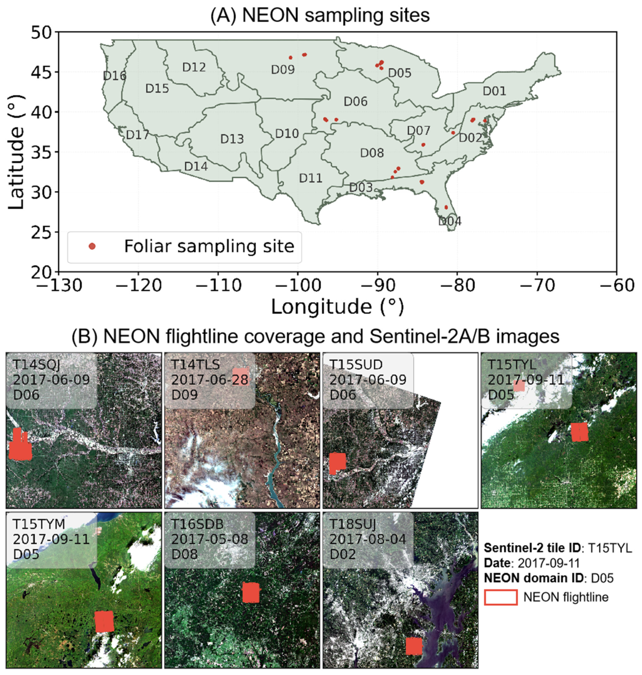
Field sampling was conducted during the 2016–2017 growing seasons following National Ecological Observatory Network (NEON) vegetation sampling protocols. The field campaigns at each site were conducted within two weeks of the corresponding NEON-AOP overflights, ensuring temporal consistency between field measurements and airborne observations (Figure 1A) [16]. These sites span a broad climatic gradient across the eastern United States, encompassing humid continental, humid subtropical, and temperate grassland environments. Mean annual temperature across the sampled sites ranges from 4.3 to 17.2 °C, while mean annual precipitation ranges from 457 to 1383 mm, reflecting substantial variability in climatic conditions among the study locations.

In total, 634 sampling plots (~5 × 5 m²) were established to collect foliar samples from seven NEON ecological domains (D02, D03, D05, D06, D07, D08, and D09). The geographic coordinates of each sampling plot were precisely recorded using a differential global positioning system (GPS) (Trimble Geo 7X; Trimble Inc., Sunnyvale, CA, USA) to ensure accurate spatial alignment between field measurements and NEON imaging spectroscopy observations. The sampling plots represented six plant functional types (PFTs), including broadleaf trees (n = 432), conifers (n = 74), shrubs (n = 33), grasses (n = 61), forbs (n = 25), and crops (n = 9). The sampling sites encompassed a wide range of ecosystems, including eastern deciduous forests (SERC), northern mixed hardwood–conifer forests (CHEQ, STEI, and UNDE), tallgrass prairie and old-field grasslands (KONZ and UKFS), southeastern mixed pine–hardwood forests (TALL), and northern mixed-grass prairie with wetlands and agricultural vegetation (NOGP). This diversity of vegetation communities provided a broad range of canopy structures and foliar phenolic characteristics for model development. A complete list of the plant species sampled at each NEON site is provided in Supplementary Table S1.

Leaf sampling was conducted following NEON vegetation sampling protocols to obtain representative foliar trait measurements [16]. For each plot, sunlit and healthy leaves were collected from representative vegetation individuals, with multiple samples collected when necessary to account for within-plot variability. Sampling strategies were adjusted according to vegetation structure and growth form, including species-level sampling for woody vegetation and representative community sampling for herbaceous and mixed-species plots. Then, leaves were oven-dried at 65 °C for at least 48 h and subsequently analyzed for total phenolics concentration following the established protocol [44]. Finally, community-weighted mean (CWM) phenolic concentrations were calculated by aggregating species-level phenolic values according to species composition and relative abundance within each plot [16]. Since broadleaf tree plots were mainly occupied by one species, the CWM was typically represented by the dominant canopy species. In conifer plots, species-level phenolic concentrations were weighted according to the relative proportions of different needle age classes visually identified for each sampling branch. For shrub, grass, and forb communities, species-level phenolic concentrations were combined using species fractional cover within each plot. The resulting plot-level CWM phenolic concentrations were then paired with canopy reflectance extracted from the corresponding NEON-AOP imagery for model development.

2.2. NEON Airborne Observation Platform Imaging Spectroscopy Data

Airborne imaging spectroscopy data were obtained from the NEON Airborne Observation Platform (AOP) for the corresponding sampling plots. The AOP imaging spectrometer collects hyperspectral radiance data across 426 spectral bands spanning 380–2520 nm, with approximately 5 nm spectral resolution and 1 m spatial resolution. The data were radiometrically calibrated, atmospherically corrected, and ortho-rectified to generate surface reflectance products [45]. Wavelength regions strongly affected by atmospheric absorption and low signal-to-noise ratios (381–412, 1338–1454, 1784–1980, and 2400–2511 nm) were excluded. A Savitzky–Golay filter with a window size of 7 bands was applied to smooth spectral data within the VNIR (415–1335 nm) and SWIR (1460–1780 nm and 1990–2350 nm) wavelength regions separately. To minimize the differences in brightness, NEON spectra were vector-normalized to unit vectors [46]. The surface reflectance imagery covering the field sampling plots was extracted for foliar phenolics estimation using GPS data. Vegetation pixels within each plot were averaged to obtain representative spectral signatures, which were subsequently used for foliar phenolics modeling (Section 2.4). All spatial datasets, including NEON AOP imagery, Sentinel-2 imagery, and field plot locations, were processed in the Universal Transverse Mercator (UTM) coordinate reference system using the corresponding UTM zone for each study site to ensure consistent spatial alignment during data processing and analysis.

To facilitate upscaling of fine-resolution foliar phenolics estimates to Sentinel-2 observations, additional NEON AOP flightlines during 2017 were selected based on their spatial overlap with Sentinel-2 tiles and the availability of temporally matched Sentinel-2 acquisitions (Figure 1B; Table S2). In total, seven Sentinel-2 tiles covering corresponding NEON sites across five ecological domains (D02, D05, D06, D08, and D09) were included. These tiles corresponded to NEON sites including KONZ (Site full name: Konza Prairie Biological Station; NEON domain ID: D06; Sentinel tile ID: T14SQJ), NOGP (Northern Great Plains Research Station; D09; T14TLS), UKFS (University of Kansas Field Station; D06; T15SUD), CHEQ (Chequamegon Ecosystem-Atmosphere Study Site) and STEI (Steigerwaldt-Chequamegon Experimental Forest; D05; T15TYL), UNDE (University of Notre Dame Environmental Research Center; D05; T15TYM), TALL (Talladega National Forest; D08; T16SDB), and SERC (Smithsonian Environmental Research Center; D02; T18SUJ). The selected Sentinel-2 tiles contained 17–37 available AOP flightlines, which provided multiple airborne observations for generating fine-resolution foliar phenolics estimates. These 1 m resolution phenolics maps were subsequently used to extract ROI (Regions-Of-Interest)-level mean phenolic concentrations across multiple window sizes for evaluating cross-scale transferability (Section 2.5). Instead of mosaicking overlapping flightlines, each flightline was processed independently to extract ROI-level mean phenolics.

2.3. Sentinel-2 Multispectral Data

Sentinel-2 multispectral imagery was acquired from the Copernicus Sentinel-2 mission to support the upscaling of fine-resolution foliar phenolics estimates from NEON AOP observations to satellite spatial resolution (Figure 1B). Level-2A surface reflectance products were obtained for seven Sentinel-2 tiles (T14SQJ, T14TLS, T15SUD, T15TYL, T15TYM, T16SDB, and T18SUJ) corresponding to the NEON sites used in this study. The selected Sentinel-2 observations were acquired between May and September 2017 and were selected to closely match the available NEON-AOP acquisitions. The temporal differences between paired NEON-AOP and Sentinel-2 observations ranged from −6 to +10 days (Table S2), reducing potential discrepancies associated with short-term phenological changes.

The Level-2A products provide atmospherically corrected surface reflectance measurements across the visible, red-edge, near-infrared (NIR), and shortwave infrared (SWIR) regions. Nine Sentinel-2 spectral bands were used in this study, including the visible bands (B02, B03, and B04), red-edge bands (B05, B06, and B07), NIR band (B8A), and SWIR bands (B11 and B12), covering wavelengths from 490 to 2190 nm. The original 20 m resolution bands (B05, B06, B07, B8A, B11, and B12) were resampled to 10 m to match the spatial resolution of the native 10 m bands (B02–B04). Cloud-contaminated pixels were removed using the Sentinel-2 cloud probability (CLD) product to ensure that only clear-sky observations were retained for subsequent analysis.

2.4. Foliar Phenolics Modeling Using NEON Imaging Spectroscopy

Foliar phenolics were modeled by linking NEON imaging spectroscopy data (Section 2.2) with laboratory-measured foliar phenolic concentrations (Section 2.1). The dataset was divided into calibration (75%) and validation (25%) subsets using stratified sampling based on PFTs to ensure that all vegetation functional groups were represented in both datasets. Two complementary regression approaches were evaluated to characterize potential linear and nonlinear relationships between canopy reflectance and foliar phenolics, including partial least squares regression (PLSR) and Gaussian process regression (GPR).

PLSR was implemented as a linear modeling approach that reduces spectral dimensionality by transforming correlated reflectance variables into a set of latent components. The optimal number of latent components was determined using repeated cross-validation (4 folds; 25 repeats) on the calibration dataset. GPR was implemented as a nonlinear regression approach, with model calibration performed using the same repeated cross-validation strategy and a radial basis function kernel to capture nonlinear relationships between spectral reflectance and foliar phenolic concentrations. To account for variability associated with model calibration, 100 models were generated from the repeated cross-validation procedure. Predictions were obtained as the ensemble mean of the 100 models, and the standard deviation among model predictions was used to quantify prediction uncertainty. Both PLSR and GPR models were independently evaluated using the same validation dataset, and model performance was assessed using the coefficient of determination (R²), root mean square error (RMSE, in mg·g⁻¹), and normalized root mean square error (NRMSE = RMSE/(Max − Min) × 100%, in %).

To identify spectral regions associated with foliar phenolics, wavelength importance was evaluated for both PLSR and GPR models. For PLSR, standardized regression coefficients from the repeated cross-validation models were extracted, and the mean coefficient value across all models was calculated for each wavelength. The magnitude and sign of the coefficients were used to characterize the contribution and direction of spectral bands to phenolics prediction. For GPR, wavelength importance was quantified based on the automatic relevance determination (ARD) length scales derived from the radial basis function kernel. The inverse length scale was calculated, with larger values indicating greater sensitivity of the model to specific wavelengths. Known vegetation biochemical absorption regions were additionally indicated to facilitate interpretation of model-identified spectral features in relation to reported foliar chemical absorption characteristics [24].

2.5. Foliar Phenolics Modeling Using Sentinel-2 Multispectral Data

2.5.1. Generation of AOP-Derived Phenolics Reference Data

The optimized NEON hyperspectral phenolics models (Section 2.4) were first applied to available NEON Airborne Observation Platform (AOP) flightlines (Section 2.2 and Figure 1B) to generate spatially continuous foliar phenolics estimates at 1 m spatial resolution. These AOP-derived phenolics maps provided fine-resolution trait information within Sentinel-2 coverage areas and served as reference data for satellite-scale upscaling.

To address potential spatial misalignment between NEON AOP-derived phenolics estimates and Sentinel-2 observations, multiple spatial aggregation windows were evaluated. Although AOP imagery provides fine-resolution (1 m) phenolics estimates, direct pixel-to-pixel matching with Sentinel-2 imagery is challenging because of differences in spatial resolution, geolocation accuracy, and sensor acquisition geometry. Therefore, square regions of interest (ROIs) with four window sizes (10, 20, 60, and 100 NEON AOP pixels) were generated around the same center locations for each NEON AOP flightline. These window sizes were selected to evaluate the effects of increasing aggregation scale on cross-sensor phenolics estimation. The 10 m and 20 m windows represented aggregation levels close to the native spatial resolutions of Sentinel-2 observations, while the 60 m and 100 m windows evaluated broader aggregation scales where canopy heterogeneity, geolocation mismatch, and differences between airborne and satellite observations were expected to be reduced. The 100 m window further represented a landscape-level aggregation scale commonly used in ecosystem remote sensing and trait mapping studies.

To ensure reliable aggregation of AOP-derived phenolics estimates, each ROI was required to contain more than 80% valid vegetation pixels, where valid pixels were defined as pixels with NDVI > 0.6 and valid phenolics predictions. In addition, ROIs were spatially separated to minimize the influence of spatial autocorrelation among samples. Specifically, the centers of the 100 × 100-pixel windows were required to be separated by more than 1.5 km. These criteria ensured that extracted ROI samples represented independent spatial observations while maintaining sufficient vegetation coverage. For each ROI, the mean AOP-derived phenolics concentration was calculated and used as the reference value for corresponding Sentinel-2 observations.

2.5.2. Sentinel-2 Spectral Feature Construction

Sentinel-2 spectral features were constructed from atmospherically corrected surface reflectance data to capture spectral information related to foliar phenolics. Three categories of predictors were generated, including: (1) raw spectral reflectance; (2) published vegetation indices; and (3) normalized difference spectral indices (NDSIs) (

Table 1. Sentinel-2 spectral features used for foliar phenolics modeling.

Feature Group	Feature	Formula	Information
Raw spectral reflectance	B02	ρ2	Blue (490 nm)
	B03	ρ3	Green (560 nm)
	B04	ρ4	Red (665 nm)
	B05	ρ5	Red-edge 1 (705 nm)
	B06	ρ6	Red-edge 2 (740 nm)
	B07	ρ7	Red-edge 3 (783 nm)
	B8A	ρ8A	NIR (865 nm)
	B11	ρ11	SWIR1 (1610 nm)
	B12	ρ12	SWIR2 (2190 nm)
Published vegetation indices	NDVI	(ρ8A − ρ4)/(ρ8A + ρ4)	Normalized Difference Vegetation Index
	EVI	2.5(ρ8A − ρ4)/(ρ8A + 6ρ4 − 7.5ρ2 + 1)	Enhanced Vegetation Index
	NDRE	(ρ8A − ρ5)/(ρ8A + ρ5)	Normalized Difference Red Edge Index
	NDRE1	(ρ6 − ρ4)/(ρ6 + ρ4)	Normalized Difference Red Edge Index 1
	NDRE2	(ρ7 − ρ4)/(ρ7 + ρ4)	Normalized Difference Red Edge Index 2
	MTCI	(ρ6 − ρ5)/(ρ6 + ρ5)	MERIS Terrestrial Chlorophyll Index
	CIred-edge	ρ7/ρ5 − 1	Chlorophyll Index Green
	CIgreen	ρ7/ρ3 − 1	Chlorophyll Index Red Edge
	NDMI	(ρ8A − ρ11)/(ρ8A + ρ11)	Normalized Difference Moisture Index
	SIPI	(ρ8A − ρ4)/(ρ8A − ρ5)	Structure Insensitive Pigment Index
	ARI	(1/ρ3 − 1/ρ5) × ρ7	Anthocyanin Reflectance Index
	PSRI	(ρ4 − ρ2)/ρ6	Plant Senescence Reflectance Index
	REP	ρ8A + 35[((ρ4 + ρ7)/2 − ρ5)/(ρ6 − ρ5)]	Red Edge Position
Normalized difference spectral indices (NDSIs)	NDSIij	(ρi − ρj)/(ρi + ρj)	All Sentinel-2 band pairs

).

Raw spectral reflectance features consisted of nine Sentinel-2 bands, including visible bands (B02, B03, and B04), red-edge bands (B05, B06, and B07), near-infrared band (B8A), and shortwave infrared bands (B11 and B12). These bands were retained because visible, red-edge, and near-infrared regions are sensitive to vegetation pigment and canopy structural properties, whereas shortwave infrared regions provide information related to vegetation water content and dry matter constituents [14].

Published vegetation indices were calculated to enhance vegetation-related signals and summarize specific canopy properties. A total of 13 vegetation indices were generated, including indices related to vegetation greenness (e.g., NDVI and EVI), chlorophyll status (e.g., CI_green, CIred-edge, and MTCI), pigment variation (e.g., ARI and SIPI), and water status (e.g., NDMI). The formulas and corresponding Sentinel-2 bands used for each index are provided in Table 1.

In addition, normalized difference spectral indices (NDSIs) were generated to capture pairwise spectral relationships among Sentinel-2 bands. For each possible band pair, NDSI values were calculated as:

$$NDS{I}_{ij}={\displaystyle \frac{{\rho }_i-{\rho }_j}{{\rho }_i+{\rho }_j}}$$

where ${\rho }_i$ and ${\rho }_j$ represent Sentinel-2 surface reflectance values at spectral bands i and j, respectively. These band combinations provide additional information on spectral contrasts that may be associated with foliar biochemical variation. Six NDSI combinations corresponding to commonly used normalized difference vegetation indices (NDVI, NDRE, NDRE1, NDRE2, MTCI, and NDMI in Table 1) were excluded to avoid exact duplication with published vegetation indices. Therefore, 30 independent NDSI features were retained. The final Sentinel-2 predictor dataset consisted of nine reflectance bands, 13 vegetation indices, and 30 NDSI features.

2.5.3. Sentinel-2 Phenolics Modeling and Validation

The ROI datasets were randomly divided into calibration (75%) and validation (25%) subsets. Model development was conducted independently for each ROI size (10, 20, 60, and 100 pixels) to evaluate the influence of spatial aggregation on Sentinel-2-based phenolics estimation.

Three modeling approaches were evaluated, including partial least squares regression (PLSR), Gaussian process regression (GPR), and random forest (RF) regression. PLSR was used to characterize linear relationships between Sentinel-2 spectral features and foliar phenolics concentrations, whereas GPR and RF were used to capture potential nonlinear relationships. For PLSR and GPR, model calibration was performed using repeated cross-validation (4 folds; 25 repeats). In PLSR, the optimal number of latent components was selected based on cross-validation performance, while GPR employed a radial basis function kernel to model nonlinear spectral–trait relationships. RF models were implemented as ensemble regression trees using bootstrap aggregation.

Model performance was evaluated on the independent validation dataset using R², RMSE (mg·g⁻¹), and NRMSE (%). Model performance was compared across ROI sizes and modeling approaches to identify the optimal configuration for Sentinel-2-based phenolics estimation.

Following model evaluation, the best-performing model developed from the 100-pixel ROI dataset was selected for regional phenolics mapping. The selected model was applied to Sentinel-2 Level-2A imagery using the same set of spectral features used during model training, generating spatially continuous estimates of foliar phenolics across the study regions.

All data processing, statistical analyses, and model development were implemented in Python 3.12.2. Numerical computations and data management were performed using NumPy (v1.26.4), pandas (v2.2.2), and SciPy (v1.17.1). Geospatial processing was conducted using rasterio (v1.4.3), GDAL (v3.6.2), GeoPandas (v1.0.1), Shapely (v2.1.2), and pyproj (v3.6.1). Partial least squares regression (PLSR) and random forest regression (RFR) were implemented using scikit-learn (v1.5.1), while Gaussian process regression (GPR) was implemented using GPy (v1.13.2). Figures were generated using Matplotlib (v3.8.4).

3. Results

3.1. Variability of Foliar Phenolics and Canopy Reflectance Across Plant Functional Types

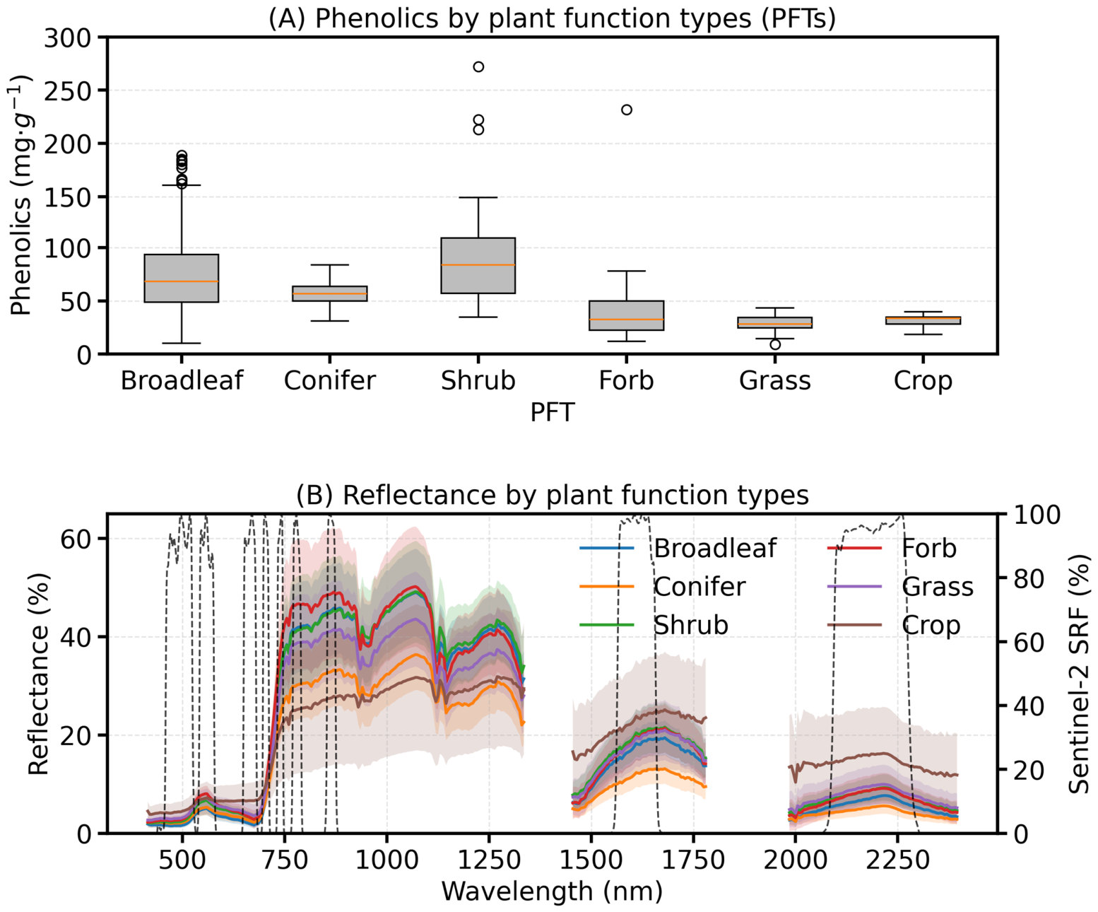
Foliar phenolics exhibited substantial variability across plant functional types (PFTs), reflecting strong functional differences in secondary metabolite allocation (Figure 2A). Shrubs showed the highest mean phenolic concentration (91.07 ± 55.78 mg·g⁻¹), followed by broadleaf trees (75.30 ± 35.38 mg·g⁻¹) and conifers (57.15 ± 11.16 mg·g⁻¹). Herbaceous vegetation exhibited comparatively lower concentrations, with forbs (43.54 ± 42.98 mg·g⁻¹) and crops (31.65 ± 6.56 mg·g⁻¹) showing intermediate levels, while grasses displayed the lowest mean values (29.33 ± 7.39 mg·g⁻¹). Across PFTs, phenolic distributions spanned wide ranges, particularly in shrubs (34.63–271.97 mg·g⁻¹) and forbs (12.18–231.67 mg·g⁻¹), indicating strong intra-functional variability. In contrast, conifers and grasses exhibited comparatively narrower ranges, suggesting more constrained biochemical variation within these functional groups.

Spectral reflectance showed clear separability among plant functional types (PFTs) across the visible (VIS), near-infrared (NIR), and shortwave infrared (SWIR) domains (Figure 2B). In the visible region (400–700 nm), all PFTs exhibited low reflectance due to strong chlorophyll absorption, with values typically ranging from 0.02 to 0.07. In the NIR region (700–1300 nm), stronger divergence emerged among PFTs. Broadleaf and shrub vegetation exhibited the highest reflectance, reaching 0.40–0.50 at peak wavelengths (around 800–900 nm), followed by conifers (0.30–0.36), while grasses and crops remained lower (0.35–0.43 for grasses; 0.25–0.32 for crops). In the SWIR region (1300–2500 nm), reflectance declined progressively due to increasing water absorption, particularly near 1400 nm and 1900 nm. Broadleaf and shrub PFTs generally maintained higher SWIR reflectance (0.20–0.30 and 0.18–0.22, respectively), compared with conifers (0.10–0.13), grasses (0.15–0.20), and crops (0.12–0.16). Overall, woody vegetation consistently showed higher reflectance in both NIR and SWIR regions compared with herbaceous PFTs, reflecting canopy structural differences and variation in leaf biochemicals.

3.2. Validation Performance and Spectral Feature Importance of NEON-Based Phenolic Prediction Models

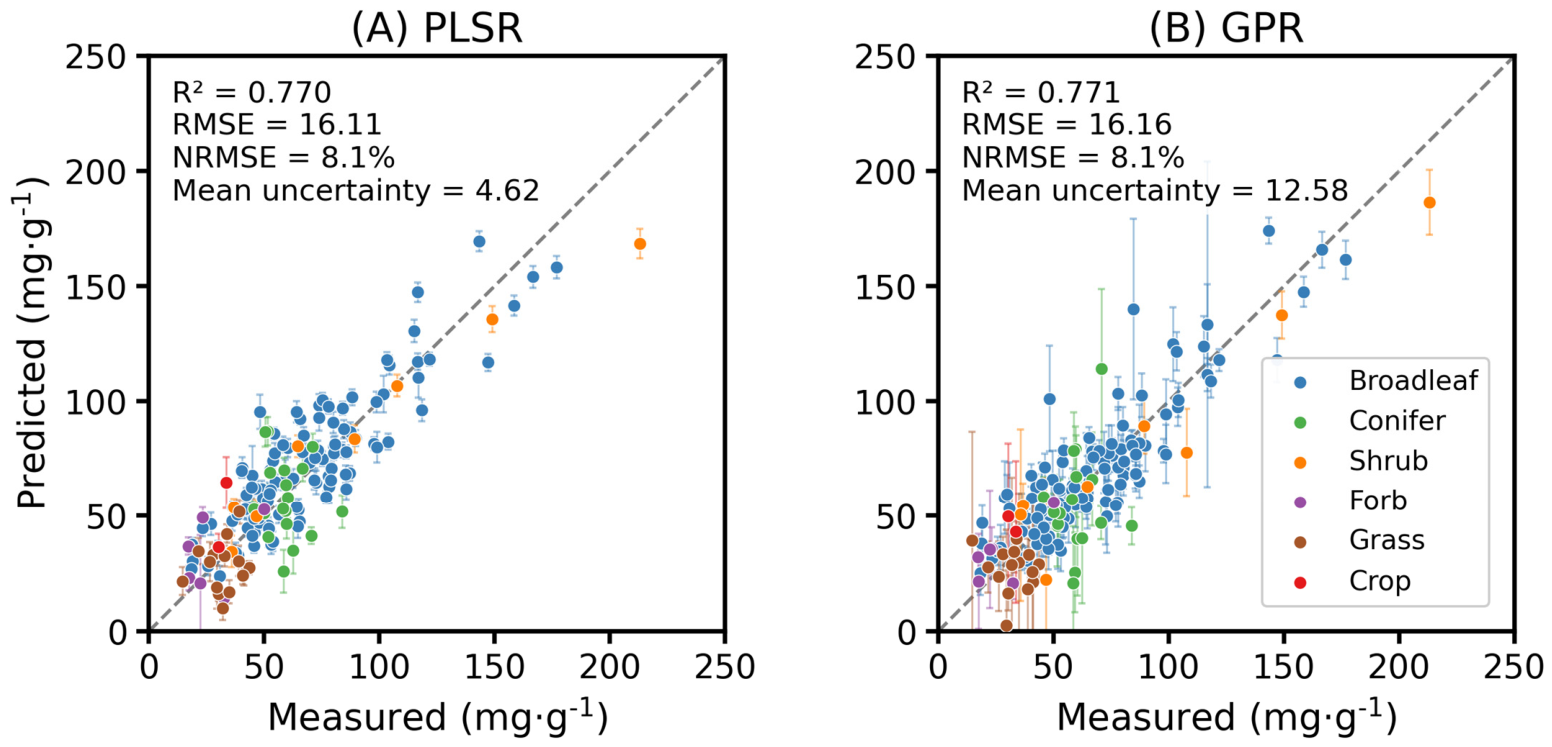
The validation performance of the NEON-based phenolic prediction models showed that both PLSR and GPR approaches achieved comparable predictive capability (Figure 3). The PLSR model resulted in an RMSE of 16.11 mg·g⁻¹ and an R² of 0.770, while the GPR model produced a similar RMSE of 16.16 mg·g⁻¹ and an R² of 0.771, indicating that both linear and nonlinear machine learning-based modeling approaches captured the major spectral–phenolic relationships across diverse plant functional types. The NRMSE values were identical for both models (8.1%), further demonstrating consistent prediction performance. Although the overall accuracy was comparable, differences were observed in prediction uncertainty. The PLSR model showed lower mean ensemble uncertainty (4.62 mg·g⁻¹) compared with the GPR model (12.58 mg·g⁻¹), suggesting more stable predictions across NEON samples.

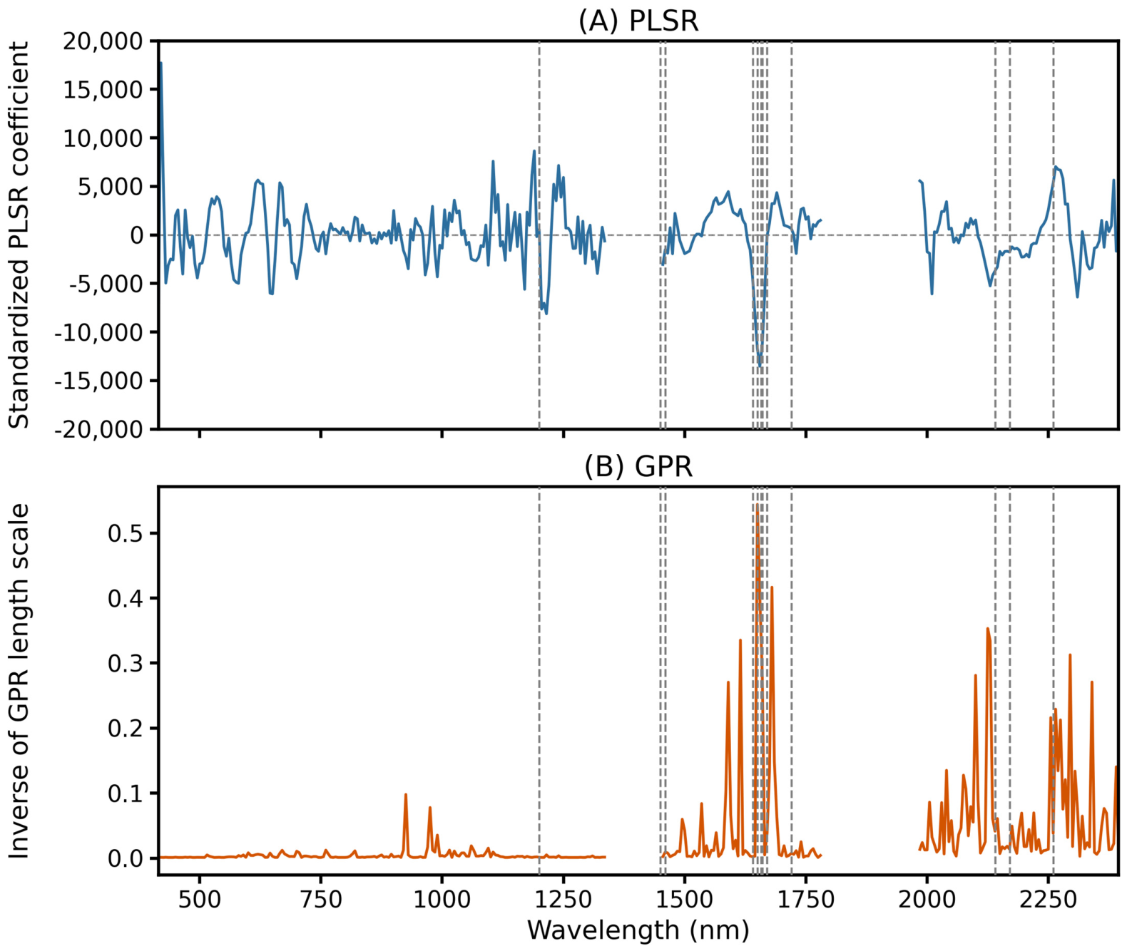
Spectral feature importance analysis revealed that both PLSR and GPR models identified several informative wavelength regions for foliar phenolic prediction (Figure 4). The PLSR coefficients showed distinct positive and negative contributions across the spectrum, indicating differential spectral responses associated with phenolic variability. Strong coefficient magnitudes were observed in the visible region, particularly around 420–550 nm, where both positive and negative responses occurred, as well as in the shortwave infrared region around 1200–1300 nm, 1450–1750 nm, and 2100–2300 nm. Notably, pronounced coefficient responses were observed near previously reported phenolic-related absorption features, including 1200, 1450–1460, 1641–1670, 1720, 2140, 2170, and 2260 nm. The GPR model showed a comparable spectral pattern, with higher inverse radial basis function length-scale importance mainly concentrated in the shortwave infrared region, particularly around 1450–1750 nm and 2100–2300 nm. Despite differences in the representation of spectral contributions between the two modeling approaches, both models highlighted similar wavelength regions, suggesting that these spectral domains provided consistent information for predicting foliar phenolic variability across NEON vegetation types.

3.3. Effects of Spatial Aggregation Scale on Sentinel-2 Phenolic Prediction Performance and Spectral Feature Importance

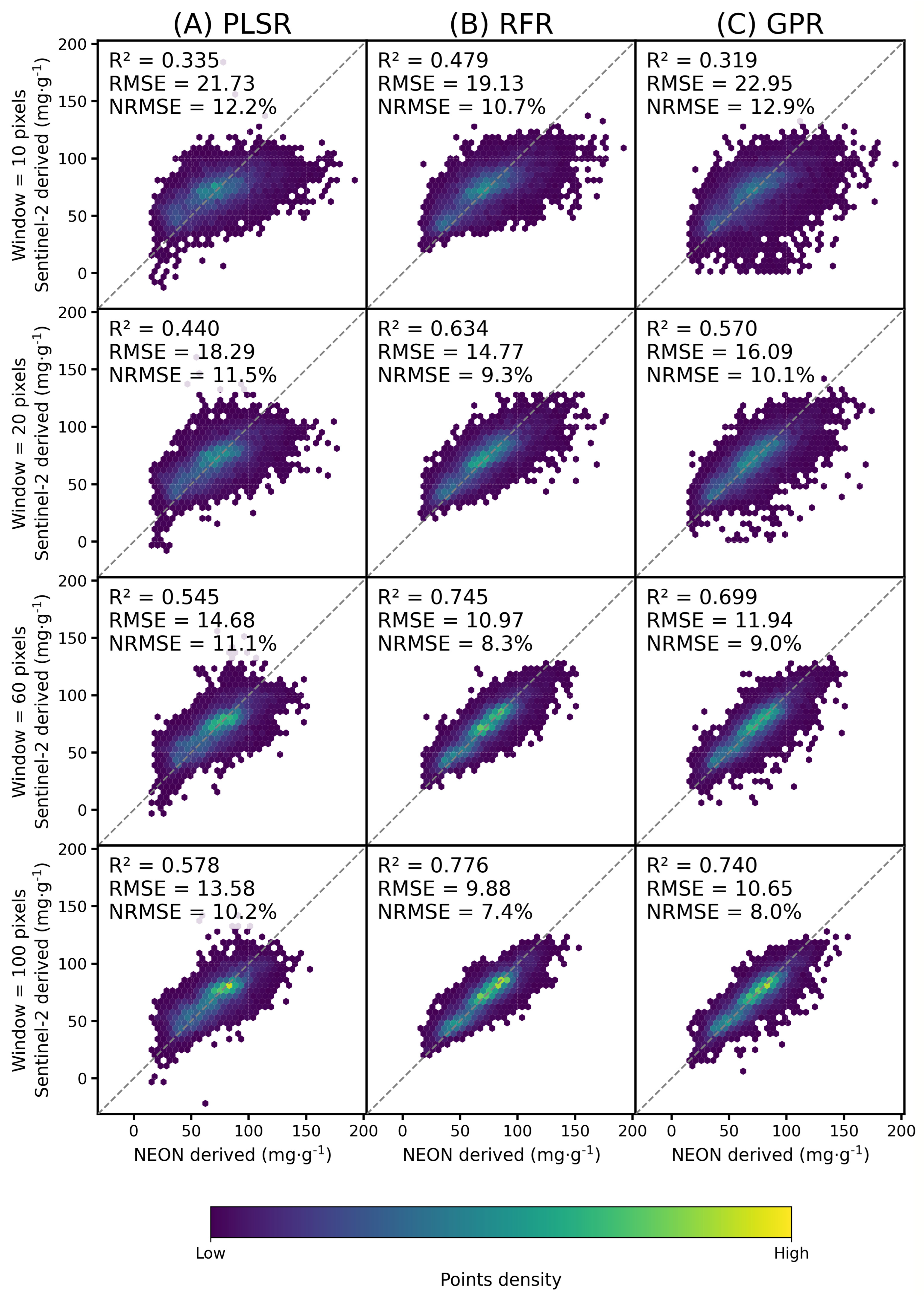
The validation performance of Sentinel-2-based foliar phenolics prediction varied substantially with ROI window size and modeling approach (Figure 5). Across all models, increasing the spatial aggregation window from 10 to 100 NEON pixels consistently improved prediction accuracy, indicating that larger spatial support enhanced the agreement between Sentinel-2 observations and NEON-derived phenolic measurements by reducing spatial scale mismatch and geolocation misalignment. The RFR model achieved the highest predictive performance, with R² increasing from 0.479 (NRMSE = 10.7%) at the 10-pixel window to 0.776 (NRMSE = 7.0%) at the 100-pixel window. The GPR model showed a similar improvement, increasing from R² = 0.319 (NRMSE = 12.9%) to R² = 0.740 (NRMSE = 8.0%) across the same range of ROI sizes. The PLSR model also improved with increasing spatial support, with R² increasing from 0.335 (NRMSE = 12.2%) to 0.578 (NRMSE = 10.2%). Across all aggregation scales, RFR consistently achieved the highest predictive accuracy, followed by GPR and PLSR, suggesting that nonlinear machine learning-based modeling approaches were better able to capture complex spectral–phenolic relationships in Sentinel-2 observations.

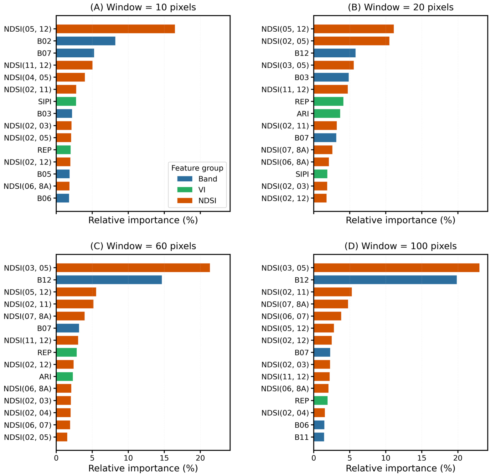
Feature importance analysis of the RFR models revealed that the contribution of spectral predictors varied with ROI window size (Figure 6). Across all spatial scales, normalized difference spectral indices (NDSIs) represented the dominant predictors of foliar phenolic variability, accounting for most of the top-ranked features. At the smallest window size (10 pixels), NDSIB05 and B12 showed the highest importance (16.5%), followed by several visible- and shortwave infrared-based NDSIs. With increasing spatial aggregation, the dominant features shifted toward stronger contributions from SWIR-related spectral information. At the 60- and 100-pixel windows, NDSIB03 and B05 became the most important predictors, accounting for 21.3% and 23.0% of total importance, respectively, while B12 reflectance (at 2190 nm) increased substantially in importance, reaching 14.7% and 19.9% at these two spatial scales. In contrast, vegetation indices such as REP, SIPI, and ARI remained consistently selected across different window sizes but generally contributed less than NDSI-based features. These results suggest that spatial aggregation influenced the spectral features used by RFR models, with larger ROI windows emphasizing stable red-edge and SWIR spectral signals associated with foliar phenolic variability.

3.4. Spatial Consistency Between Sentinel-2 and NEON Imaging Spectroscopy Phenolic Estimates

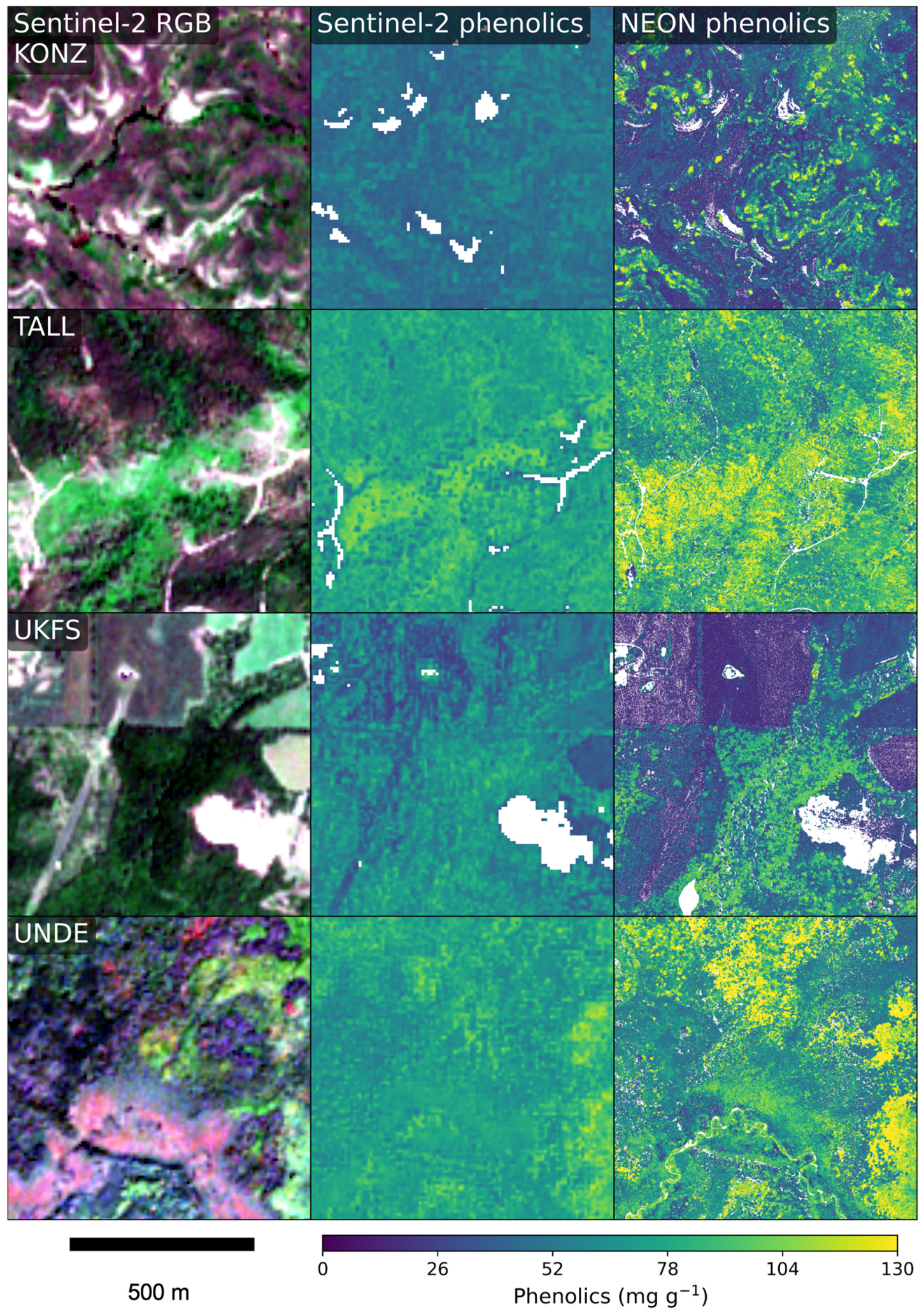
Visual comparison of phenolic maps derived from Sentinel-2 and NEON imaging spectroscopy showed that Sentinel-2 predictions captured broad spatial patterns of foliar phenolic variability across all four study sites (Figure 7). Regions with relatively high and low phenolic concentrations generally exhibited consistent spatial organization between datasets, indicating that the Sentinel-2-based model was able to reproduce large-scale phenolic gradients. This agreement was particularly evident at TALL and UNDE, where major areas of elevated phenolic content appeared in comparable locations in both products.

However, Sentinel-2-derived phenolic maps appeared substantially smoother and showed reduced fine-scale spatial variability relative to NEON estimates. Fine spatial structures and localized phenolic hotspots visible in NEON imagery were often generalized in Sentinel-2 predictions, especially at KONZ and UKFS. This smoother spatial pattern likely reflects the limited spatial and spectral resolution of Sentinel-2 compared with airborne imaging spectroscopy. In particular, the prediction model relied heavily on Sentinel-2 bands with native 20 m spatial resolution that were resampled to 10 m, as well as vegetation indices derived from these bands (Figure 6), resulting in an effective spatial support larger than the output pixel size. Consequently, the Sentinel-2 product preserved regional-scale phenolic patterns but was less capable of resolving local heterogeneity captured by NEON imaging spectroscopy.

4. Discussion

This study evaluated the feasibility of scaling foliar phenolics from airborne imaging spectroscopy to Sentinel-2 multispectral imagery across diverse vegetation types. Using the full spectral information from the airborne platform, both Partial Least Squares Regression (PLSR) and Gaussian Processes Regression (GPR) accurately predicted foliar phenolics and successfully distinguished the characteristic absorption features of these compounds. The resulting fine-resolution airborne phenolic maps served as a high-quality training dataset for upscaling to broader spatial extents with Sentinel-2. An optimal window size of 100 m was identified for matching the airborne-derived phenolic maps to Sentinel-2 pixels, effectively reducing geolocation mismatches between the two sensors. The foliar phenolic maps generated from the hyperspectral airborne data and the upscaled Sentinel-2 multispectral imagery showed strong spatial consistency across heterogeneous landscapes.

4.1. Accurate Prediction of Foliar Phenolics Across Vegetation Types Using Airborne Imaging Spectroscopy

Imaging spectroscopy demonstrated the ability to capture the variation in foliar phenolics from leaf to canopy levels [17,23,24,28,47]. Our findings further confirmed the feasibility of airborne imaging spectroscopy for accurately predicting foliar phenolics across a wide range of vegetation types including trees, shrubs and graminoids. The estimation accuracies achieved in this study were comparable to or higher than those reported in previous studies [16,17,18,29]. We found that the widely used PLSR, which captured linear relationships between foliar phenolics and canopy spectra, achieved similarly good performance with GPR, which could model the non-linear relationships. This finding is consistent with a previous study on predicting multiple foliar traits in grasslands [42], as well as a study on predicting foliar phenolics using leaf spectroscopy [24]. However, it contrasted with another study on canopy-level phenolic prediction using airborne and spaceborne imaging spectroscopy, in which GPR outperformed PLSR [29]. Careful hyperparameter optimization is critical for machine learning algorithms like GPR to achieve satisfactory estimation accuracy [43]. In our study, the prediction uncertainties associated with GPR were generally higher than those of PLSR. However, GPR offers the intrinsic advantage of providing per-pixel uncertainty estimates directly alongside predicted values, whereas PLSR must rely on a permutational approach to approximate prediction uncertainties [18,42]. Both uncertainty quantification methods are important for trait mapping, as they supply the confidence information necessary to inform and constrain subsequent trait-based analyses [16].

The underlying mechanism of predicting foliar phenolics from spectra lies in their distinct absorption features, located at approximately 1200, 1450, 1460, 1641, 1650, 1658, 1660, 1670, 1720, 2140, 2170, and 2260 nm [14,19,20,21,22]. Among these, the absorption feature centered near 1660 nm is particularly diagnostic, as it corresponds to the first overtone of aromatic C–H bond stretching—a fundamental structural signature of phenolic compounds [23]. Our results revealed that this prominent absorption feature was adequately captured by both models, as evidenced by the band importance metrics derived from each. In addition to the 1660 nm feature, PLSR also captured absorption features at 1200, 1450, 1460, 1720, and 2260 nm, whereas GPR captured a more limited set of additional features, notably those at 2140 and 2260 nm. Xie et al. [24] reported that the center wavelength of the key phenolic absorption feature may shift between 1653 and 1667 nm depending on factors such as plant species and environmental conditions. Consistent with this finding, our models identified the entire spectral region between 1650 and 1670 nm as important for predicting foliar phenolics, encompassing the range of variation expected across the diverse vegetation types, plant species, and broad geographic conditions represented in our study.

4.2. Airborne Imaging Spectroscopy as a Bridge for Scaling Foliar Phenolics to Sentinel-2

The highly accurate estimation of foliar phenolics from airborne imaging spectroscopy provided a robust foundation for scaling predictions to Sentinel-2 imagery. However, bridging the gap between field measurements and satellite observations remains challenging due to the coarse spatial resolution of satellite pixels and the inherent spatial mismatch with ground-based surveys. Previous studies have highlighted the difficulties in directly linking field measurements to airborne or satellite data [17,33]. Moreover, the requirement for both leaf traits and species abundance to compute community-weighted means adds another layer of complexity to the spectral matching process, especially in species-rich plots where taxonomic and functional diversity are high. In this study, we employed a 5 × 5 m field plot design specifically aligned with the 1 m spatial resolution of the airborne imagery, resulting in a fine-resolution phenolic map that served as a high-quality training dataset for upscaling to Sentinel-2. Among the three empirical approaches evaluated, RFR achieved the highest prediction accuracy for foliar phenolics, followed by GPR, while PLSR yielded comparatively lower accuracies. This outcome likely reflects the ability of RFR and GPR to capture the non-linear relationships between foliar phenolics and canopy spectra, which PLSR, as a linear method, may not fully represent [29,43].

Furthermore, the spatial mismatch inherent between the two data types significantly influenced model performance, as evidenced by the effect of varying the aggregation window size. A window size of 10 m—corresponding to the finest spatial resolution of Sentinel-2 imagery—yielded only moderately accurate predictions, underscoring the geolocation discrepancies between the airborne-derived phenolic maps and Sentinel-2 pixels. As the window size increased, these spatial mismatches were progressively alleviated, leading to corresponding improvements in estimation accuracy. The optimal aggregation window was found to be 100 m, a scale that effectively minimized spatial misalignment between the two datasets while preserving the spectral absorption features of foliar phenolics necessary for accurate retrieval.

The estimation accuracies of foliar phenolics derived from Sentinel-2 were comparable to those reported in previous studies and notably higher than those from a prior effort that utilized time series Sentinel-2 data for upscaling [48]. This improvement is largely attributable to the near-simultaneous acquisition of airborne and satellite imagery, which minimized temporal mismatch. By reducing the reliance on multi-temporal data, our approach is more readily transferable to other regions. We note, however, that inter- and intra-annual variation in foliar phenolics and canopy spectra can affect model performance, and the use of single-date imagery may not fully capture such dynamics [18]. The most informative spectral features were the Normalized Difference Spectral Indices (NDSI) based on the green and red-edge bands, together with the SWIR2 band. The SWIR2 band likely captures part of the phenolic absorption near 2260 nm, while the contributions from green and red-edge bands point to indirect correlations between foliar phenolics and co-varying traits such as chlorophyll and nitrogen.

Landscape-scale application of the models revealed broadly consistent spatial patterns in foliar phenolics between the airborne and Sentinel-2 maps across diverse sites. However, the fine spatial detail visible in the high-resolution airborne maps was inevitably obscured in the coarser Sentinel-2 maps, especially in areas with extreme high or low values. This is an inherent trade-off in spaceborne remote sensing between spatial and spectral resolution. The new generation of satellite imaging spectrometers—such as EnMAP, PRISMA, Gaofen-5, DESIS, and the forthcoming SBG mission—typically operate at 30 m or 60 m spatial resolutions. We expect that their enhanced spectral resolution will help offset the coarser spatial detail by better resolving the characteristic phenolic absorption features. Nevertheless, none of the current operational hyperspectral missions are designed for full global coverage. In this context, Sentinel-2 retains a distinct advantage for mapping foliar phenolics across large areas, offering both systematic global coverage and short revisit times.

Beyond demonstrating the feasibility of cross-scale phenolic mapping, the proposed framework has several potential practical applications. Spatially explicit estimates of foliar phenolic concentrations can facilitate monitoring of plant defense strategies, vegetation responses to environmental stress, and ecosystem functioning across large spatial extents [1,2,3,4]. Because foliar phenolics are closely associated with herbivory resistance, nutrient cycling, and carbon dynamics, regional phenolic maps may also support biodiversity assessments, ecological monitoring, and conservation planning. Furthermore, the integration of airborne imaging spectroscopy with freely available Sentinel-2 observations provides a scalable framework that can be readily updated as new airborne and satellite observations become available.

4.3. Limitations and Future Perspectives

Overall, our results demonstrate that the spatial variation in foliar phenolics can be accurately predicted by integrating airborne imaging spectroscopy with Sentinel-2 multispectral imagery, offering a viable pathway for scaling phenolic mapping to continental and even global extents. Nevertheless, several limitations should be acknowledged. First, although our study encompassed a relatively large number of plant species from diverse vegetation types compared to prior work, the spatial coverage remains largely confined to temperate and subtropical regions. Whether this approach can be successfully extended to tundra and tropical ecosystems, which harbor greater species diversity and more heterogeneous environmental conditions, warrants further investigation. Furthermore, although the sampled NEON sites represent a broad range of vegetation communities and climatic conditions across the eastern United States, the influence of environmental variability on phenolic retrieval performance was not explicitly quantified. Differences in climate, species composition, canopy structure, and stand characteristics may affect canopy reflectance–trait relationships and introduce additional uncertainty when transferring models across ecosystems. Although community-weighted mean phenolic concentrations were used to incorporate within-plot species composition, future studies should integrate broader environmental gradients, structural measurements, and long-term ecological observations to better evaluate model transferability.

Second, our study focused exclusively on the peak growing season; foliar phenolics, however, is known to vary across phenological stages [18]. Future research should therefore target multiple growth stages, contingent on the availability of concurrent airborne and Sentinel-2 acquisitions.

Third, the airborne imaging spectroscopy data and field measurements used in this study were collected in 2017, predating the launch of recent spaceborne imaging spectrometers and thereby precluding direct upscaling to these newer satellite platforms. However, the National Ecological Observatory Network (NEON) is designed as a long-term observation program spanning 30 years, which will enable concurrent measurements with current hyperspectral missions such as PRISMA and EnMAP, ultimately supporting repeated, synoptic monitoring of foliar traits at broader scales [29,49].

Another consideration is that the optimal aggregation window identified in this study should be interpreted within the context of the evaluated ecosystems, sensors, and spatial configurations. The improved performance observed at the 100 × 100 m window likely reflects a balance between reducing spatial mismatch between NEON AOP and Sentinel-2 observations and preserving meaningful variation in canopy phenolic signals. Increasing the aggregation window can reduce the effects of geolocation uncertainty, differences in spatial support between airborne and satellite observations, and fine-scale canopy heterogeneity, thereby improving agreement between the two datasets. However, excessive aggregation may also smooth local variations in vegetation composition and canopy chemistry, potentially reducing sensitivity to fine-scale ecological patterns. Therefore, the 100 m aggregation window identified here should not be considered a universal optimal scale, but rather an empirically determined scale for the NEON sites and Sentinel-2 observations evaluated in this study. Future applications across different ecosystems, spatial resolutions, and sensor configurations should evaluate multiple aggregation scales to identify the most appropriate spatial scale for trait retrieval.

Finally, Sentinel-2 phenolic predictions were evaluated against airborne-derived phenolic estimates, which themselves contain uncertainties associated with airborne retrieval models and spatial aggregation. Although increasing aggregation windows improved agreement between airborne and satellite observations, future studies should incorporate uncertainty-aware validation strategies and independent field observations to further quantify the reliability of satellite-based phenolic products. While the present study focused specifically on foliar phenolics, the methodological framework we developed is readily extendable to other foliar chemical traits, paving the way for comprehensive analyses of the links between foliar chemistry, ecosystem function, and functional diversity.

5. Conclusions

This study demonstrated that the integration of airborne imaging spectroscopy with Sentinel-2 multispectral imagery provided an effective framework for accurately predicting and mapping foliar phenolics across diverse vegetation types and spatial scales. By leveraging the high spectral resolution of airborne data to resolve characteristic phenolic absorption features—most notably the diagnostic feature near 1660 nm—and the global coverage and frequent revisit time of Sentinel-2, we successfully generated spatially consistent phenolic maps at landscape to regional extents. Both Partial Least Squares Regression and Gaussian Processes Regression achieved comparable predictive performance using airborne spectra, with the former capturing a broader suite of absorption features. When scaled to Sentinel-2, Random Forest Regression yielded the highest accuracies, reflecting the importance of capturing non-linear relationships between foliar phenolics and canopy reflectance. An optimal aggregation window of 100 m was identified to reduce spatial misalignment between the two sensors while preserving the spectral signals essential for phenolic retrieval. The broad consistency across landscapes confirms the viability of this upscaling approach for large-area applications. These findings advance trait mapping by bridging high-resolution airborne observations with globally available satellite data. Extending this framework to underrepresented biomes, multiple phenological stages, and concurrent hyperspectral satellite observations will be essential next steps. More broadly, this approach can be adapted to other foliar chemical traits, offering a pathway toward the large-scale monitoring of functional diversity and ecosystem function across U.S. temperate and subtropical ecosystems.

References

1. Bartwal, A.; Mall, R.; Lohani, P.; Guru, S.K.; Arora, S. Role of Secondary Metabolites and Brassinosteroids in Plant Defense Against Environmental Stresses. J. Plant Growth Regul. 2013, 32, 216–232. [Google Scholar] [CrossRef]
2. Reshi, Z.A.; Ahmad, W.; Lukatkin, A.S.; Javed, S.B. From Nature to Lab: A Review of Secondary Metabolite Biosynthetic Pathways, Environmental Influences, and In Vitro Approaches. Metabolites 2023, 13, 895. [Google Scholar] [CrossRef]
3. Verma, N.; Shukla, S. Impact of Various Factors Responsible for Fluctuation in Plant Secondary Metabolites. J. Appl. Res. Med. Aromat. Plants 2015, 2, 105–113. [Google Scholar] [CrossRef]
4. Anulika, N.P.; Ignatius, E.O.; Raymond, E.S.; Osasere, O.-I.; Abiola, A.H. The Chemistry Of Natural Product: Plant Secondary Metabolites. Int. J. Technol. Enhanc. Emerg. Eng. Res. 2016, 4, 1–8. [Google Scholar]
5. Harborne, J.B.; Williams, C.A. Advances in Flavonoid Research since 1992. Phytochemistry 2000, 55, 481–504. [Google Scholar] [CrossRef] [PubMed]
6. Scalbert, A.; Manach, C.; Morand, C.; Rémésy, C.; Jiménez, L. Dietary Polyphenols and the Prevention of Diseases. Crit. Rev. Food Sci. Nutr. 2005, 45, 287–306. [Google Scholar] [CrossRef] [PubMed]
7. Zargoosh, Z.; Ghavam, M.; Bacchetta, G.; Tavili, A. Effects of Ecological Factors on the Antioxidant Potential and Total Phenol Content of Scrophularia Striata Boiss. Sci. Rep. 2019, 9, 16021. [Google Scholar] [CrossRef] [PubMed]
8. Eugenia Aguero, M.; Gevens, A.; Nicholson, R.L. Interaction of Cochliobolus heterostrophus with Phytoalexin Inclusions in Sorghum bicolor. Physiol. Mol. Plant Pathol. 2002, 61, 267–271. [Google Scholar] [CrossRef]
9. Madritch, M.D.; Jordan, L.M.; Lindroth, R.L. Interactive Effects of Condensed Tannin and Cellulose Additions on Soil Respiration. Can. J. For. Res. 2007, 37, 2063–2067. [Google Scholar] [CrossRef]
10. Madritch, M.D.; Lindroth, R.L. Condensed Tannins Increase Nitrogen Recovery by Trees Following Insect Defoliation. New Phytol. 2015, 208, 410–420. [Google Scholar] [CrossRef] [PubMed]
11. Jan, R.; Asaf, S.; Numan, M.; Lubna; Kim, K.-M. Plant Secondary Metabolite Biosynthesis and Transcriptional Regulation in Response to Biotic and Abiotic Stress Conditions. Agronomy 2021, 11, 968. [Google Scholar] [CrossRef]
12. Zhan, X.; Chen, Z.; Chen, R.; Shen, C. Environmental and Genetic Factors Involved in Plant Protection-Associated Secondary Metabolite Biosynthesis Pathways. Front. Plant Sci. 2022, 13, 877304. [Google Scholar] [CrossRef] [PubMed]
13. Öztürk, A.; Demirsoy, L.; Demirsoy, H.; Asan, A.; Gül, O. Phenolic Compounds and Chemical Characteristics of Pears (Pyrus communis L.). Int. J. Food Prop. 2015, 18, 536–546. [Google Scholar] [CrossRef]
14. Curran, P.J. Remote Sensing of Foliar Chemistry. Remote Sens. Environ. 1989, 30, 271–278. [Google Scholar] [CrossRef]
15. Ustin, S.L.; Gitelson, A.A.; Jacquemoud, S.; Schaepman, M.; Asner, G.P.; Gamon, J.A.; Zarco-Tejada, P. Retrieval of Foliar Information About Plant Pigment Systems from High Resolution Spectroscopy. Remote Sens. Environ. 2009, 113, S67–S77. [Google Scholar] [CrossRef]
16. Wang, Z.; Chlus, A.; Geygan, R.; Ye, Z.; Zheng, T.; Singh, A.; Couture, J.J.; Cavender-Bares, J.; Kruger, E.L.; Townsend, P.A. Foliar Functional Traits from Imaging Spectroscopy across Biomes in Eastern North America. New Phytol. 2020, 228, 494–511. [Google Scholar] [CrossRef] [PubMed]
17. Asner, G.P.; Martin, R.E.; Anderson, C.B.; Knapp, D.E. Quantifying Forest Canopy Traits: Imaging Spectroscopy versus Field Survey. Remote Sens. Environ. 2015, 158, 15–27. [Google Scholar] [CrossRef]
18. Chlus, A.; Townsend, P.A. Characterizing Seasonal Variation in Foliar Biochemistry with Airborne Imaging Spectroscopy. Remote Sens. Environ. 2022, 275, 113023. [Google Scholar] [CrossRef]
19. Elvidge, C.D. Visible and near Infrared Reflectance Characteristics of Dry Plant Materials. Int. J. Remote Sens. 1990, 11, 1775–1795. [Google Scholar] [CrossRef]
20. Soukupova, J.; Rock, B.N.; Albrechtova, J. Spectral Characteristics of Lignin and Soluble Phenolics in the Near Infrared—A Comparative Study. Int. J. Remote Sens. 2002, 23, 3039–3055. [Google Scholar] [CrossRef]
21. Ben-Dor, E.; Inbar, Y.; Chen, Y. The Reflectance Spectra of Organic Matter in the Visible Near-Infrared and Short Wave Infrared Region (400–2500 Nm) during a Controlled Decomposition Process. Remote Sens. Environ. 1997, 61, 1–15. [Google Scholar] [CrossRef]
22. Ferwerda, J.G.; Skidmore, A.K.; Stein, A. A Bootstrap Procedure to Select Hyperspectral Wavebands Related to Tannin Content. Int. J. Remote Sens. 2006, 27, 1413–1424. [Google Scholar] [CrossRef]
23. Kokaly, R.F.; Skidmore, A.K. Plant Phenolics and Absorption Features in Vegetation Reflectance Spectra near 1.66 μm. Int. J. Appl. Earth Obs. Geoinf. 2015, 43, 55–83. [Google Scholar] [CrossRef]
24. Xie, R.; Darvishzadeh, R.; Skidmore, A.; Van Der Meer, F. Characterizing Foliar Phenolic Compounds and Their Absorption Features in Temperate Forests Using Leaf Spectroscopy. ISPRS J. Photogramm. Remote Sens. 2024, 212, 338–356. [Google Scholar] [CrossRef]
25. Nakaji, T.; Oguma, H.; Nakamura, M.; Kachina, P.; Asanok, L.; Marod, D.; Aiba, M.; Kurokawa, H.; Kosugi, Y.; Kassim, A.R.; et al. Estimation of Six Leaf Traits of East Asian Forest Tree Species by Leaf Spectroscopy and Partial Least Square Regression. Remote Sens. Environ. 2019, 233, 111381. [Google Scholar] [CrossRef]
26. Chen, L.; Zhang, Y.; Nunes, M.H.; Stoddart, J.; Khoury, S.; Chan, A.H.Y.; Coomes, D.A. Predicting Leaf Traits of Temperate Broadleaf Deciduous Trees from Hyperspectral Reflectance: Can a General Model Be Applied across a Growing Season? Remote Sens. Environ. 2022, 269, 112767. [Google Scholar] [CrossRef]
27. Couture, J.J.; Singh, A.; Rubert-Nason, K.F.; Serbin, S.P.; Lindroth, R.L.; Townsend, P.A. Spectroscopic Determination of Ecologically Relevant Plant Secondary Metabolites. Methods Ecol. Evol. 2016, 7, 1402–1412. [Google Scholar] [CrossRef]
28. Skidmore, A.K.; Ferwerda, J.G.; Mutanga, O.; Van Wieren, S.E.; Peel, M.; Grant, R.C.; Prins, H.H.T.; Balcik, F.B.; Venus, V. Forage Quality of Savannas—Simultaneously Mapping Foliar Protein and Polyphenols for Trees and Grass Using Hyperspectral Imagery. Remote Sens. Environ. 2010, 114, 64–72. [Google Scholar] [CrossRef]
29. Xie, R.; Darvishzadeh, R.; Skidmore, A.K.; Van Der Meer, F.; Torres-Rodriguez, A.; Heurich, M. Mapping Canopy Phenolics in European Mixed Temperate Forests Using Air- and Space-Borne Imaging Spectroscopy. Remote Sens. Environ. 2025, 331, 115020. [Google Scholar] [CrossRef]
30. Song, Z.; Xu, C.; Luan, Q.; Li, Y. Multitemporal UAV Study of Phenolic Compounds in Slash Pine Canopies. Remote Sens. Environ. 2024, 315, 114454. [Google Scholar] [CrossRef]
31. Guanter, L.; Kaufmann, H.; Segl, K.; Foerster, S.; Rogass, C.; Chabrillat, S.; Kuester, T.; Hollstein, A.; Rossner, G.; Chlebek, C.; et al. The EnMAP Spaceborne Imaging Spectroscopy Mission for Earth Observation. Remote Sens. 2015, 7, 8830–8857. [Google Scholar] [CrossRef]
32. Pignatti, S.; Palombo, A.; Pascucci, S.; Romano, F.; Santini, F.; Simoniello, T.; Umberto, A.; Vincenzo, C.; Acito, N.; Diani, M.; et al. The PRISMA Hyperspectral Mission: Science Activities and Opportunities for Agriculture and Land Monitoring. In Proceedings of the 2013 IEEE International Geoscience and Remote Sensing Symposium—IGARSS, Melbourne, VIC, Australia, 21–26 July 2013; pp. 4558–4561. [Google Scholar]
33. Aguirre-Gutiérrez, J.; Rifai, S.; Shenkin, A.; Oliveras, I.; Bentley, L.P.; Svátek, M.; Girardin, C.A.J.; Both, S.; Riutta, T.; Berenguer, E.; et al. Pantropical Modelling of Canopy Functional Traits Using Sentinel-2 Remote Sensing Data. Remote Sens. Environ. 2021, 252, 112122. [Google Scholar] [CrossRef]
34. Aguirre-Gutiérrez, J.; Rifai, S.W.; Deng, X.; Ter Steege, H.; Thomson, E.; Corral-Rivas, J.J.; Guimaraes, A.F.; Muller, S.; Klipel, J.; Fauset, S.; et al. Canopy Functional Trait Variation across Earth’s Tropical Forests. Nature 2025, 641, 129–136. [Google Scholar] [CrossRef] [PubMed]
35. Ma, X.; Mahecha, M.D.; Migliavacca, M.; Van Der Plas, F.; Benavides, R.; Ratcliffe, S.; Kattge, J.; Richter, R.; Musavi, T.; Baeten, L.; et al. Inferring Plant Functional Diversity from Space: The Potential of Sentinel-2. Remote Sens. Environ. 2019, 233, 111368. [Google Scholar] [CrossRef]
36. Féret, J.-B.; Berger, K.; De Boissieu, F.; Malenovský, Z. PROSPECT-PRO for Estimating Content of Nitrogen-Containing Leaf Proteins and Other Carbon-Based Constituents. Remote Sens. Environ. 2021, 252, 112173. [Google Scholar] [CrossRef]
37. Féret, J.-B.; Gitelson, A.A.; Noble, S.D.; Jacquemoud, S. PROSPECT-D: Towards Modeling Leaf Optical Properties Through a Complete Lifecycle. Remote Sens. Environ. 2017, 193, 204–215. [Google Scholar] [CrossRef]
38. Asner, G.P.; Martin, R.E.; Knapp, D.E.; Tupayachi, R.; Anderson, C.B.; Sinca, F.; Vaughn, N.R.; Llactayo, W. Airborne Laser-Guided Imaging Spectroscopy to Map Forest Trait Diversity and Guide Conservation. Science 2017, 355, 385–389. [Google Scholar] [CrossRef] [PubMed]
39. Wang, Z.; Chen, J.; Zhang, J.; Tan, X.; Ali Raza, M.; Ma, J.; Zhu, Y.; Yang, F.; Yang, W. Assessing Canopy Nitrogen and Carbon Content in Maize by Canopy Spectral Reflectance and Uninformative Variable Elimination. Crop J. 2022, 10, 1224–1238. [Google Scholar] [CrossRef]
40. Liu, N.; Wagner Hokanson, E.; Hansen, N.; Townsend, P.A. Multi-Year Hyperspectral Remote Sensing of a Comprehensive Set of Crop Foliar Nutrients in Cranberries. ISPRS J. Photogramm. Remote Sens. 2023, 205, 135–146. [Google Scholar] [CrossRef]
41. Wang, Z.; Li, H.; Yang, C.; Wang, J.; Chen, F.; Liu, M. Whole-Plant Trait Networks Reveal Elevational Optimization of Resource Strategies: Integration Drives Distribution in Woody Saplings. Front. Plant Sci. 2025, 16, 1463237. [Google Scholar] [CrossRef] [PubMed]
42. Wang, Z.; Townsend, P.A.; Schweiger, A.K.; Couture, J.J.; Singh, A.; Hobbie, S.E.; Cavender-Bares, J. Mapping Foliar Functional Traits and Their Uncertainties across Three Years in a Grassland Experiment. Remote Sens. Environ. 2019, 221, 405–416. [Google Scholar] [CrossRef]
43. Verrelst, J.; Camps-Valls, G.; Muñoz-Marí, J.; Rivera, J.P.; Veroustraete, F.; Clevers, J.G.P.W.; Moreno, J. Optical Remote Sensing and the Retrieval of Terrestrial Vegetation Bio-Geophysical Properties—A Review. ISPRS J. Photogramm. Remote Sens. 2015, 108, 273–290. [Google Scholar] [CrossRef]
44. Ainsworth, E.A.; Gillespie, K.M. Estimation of Total Phenolic Content and Other Oxidation Substrates in Plant Tissues Using Folin–Ciocalteu Reagent. Nat. Protoc. 2007, 2, 875–877. [Google Scholar] [CrossRef] [PubMed]
45. National Ecological Observatory Network (NEON) Spectrometer Orthorectified Surface Bidirectional Reflectance—Mosaic (DP3.30006.002). 2024. Available online: https://data.neonscience.org/data-products/DP3.30006.002 (accessed on 24 July 2026).
46. Feilhauer, H.; Asner, G.P.; Martin, R.E.; Schmidtlein, S. Brightness-Normalized Partial Least Squares Regression for Hyperspectral Data. J. Quant. Spectrosc. Radiat. Transf. 2010, 111, 1947–1957. [Google Scholar] [CrossRef]
47. Bian, M.; Skidmore, A.K.; Schlerf, M.; Wang, T.; Liu, Y.; Zeng, R.; Fei, T. Predicting Foliar Biochemistry of Tea (Camellia sinensis) Using Reflectance Spectra Measured at Powder, Leaf and Canopy Levels. ISPRS J. Photogramm. Remote Sens. 2013, 78, 148–156. [Google Scholar] [CrossRef]
48. Liu, S.; Wang, Z.; Lin, Z.; Zhao, Y.; Yan, Z.; Zhang, K.; Visser, M.; Townsend, P.A.; Wu, J. Spectra-Phenology Integration for High-Resolution, Accurate, and Scalable Mapping of Foliar Functional Traits Using Time-Series Sentinel-2 Data. Remote Sens. Environ. 2024, 305, 114082. [Google Scholar] [CrossRef]
49. Miraglio, T.; Coops, N.C.; Wallis, C.I.B.; Crofts, A.L.; Kalacska, M.; Vellend, M.; Serbin, S.P.; Arroyo-Mora, J.P.; Laliberté, E. Mapping Canopy Traits over Québec Using Airborne and Spaceborne Imaging Spectroscopy. Sci. Rep. 2023, 13, 17179. [Google Scholar] [CrossRef] [PubMed]
Figure 1. (A) NEON ecological domains and foliar sampling plot locations in the conterminous United States. (B) NEON flightline coverage and Sentinel-2A/B multispectral images.
Remotesensing 18 02599 g001
Figure 2. Distribution of foliar phenolics (A) and mean canopy reflectance spectra (±1 standard deviation) for the six plant functional types (PFTs) (B). In panel (B), each curve represents the mean reflectance across all samples belonging to the corresponding PFT, with the Sentinel-2 spectral response (dashed lines) overlaid for comparison.
Remotesensing 18 02599 g002
Figure 3. Validation of foliar phenolics predictions derived from NEON imaging spectroscopy using partial least squares regression (PLSR; (A)) and Gaussian process regression (GPR; (B)). The validation dataset consisted of 157 samples. Predictions represent the ensemble mean from 100 models, while vertical error bars indicate the standard deviation of predictions across ensemble members. Model performance is summarized by the coefficient of determination (R2), root mean square error (RMSE, in mg·g−1), normalized RMSE (NRMSE, in %), and mean predictive uncertainty (in mg·g−1).
Remotesensing 18 02599 g003
Figure 4. Relative band importance for foliar phenolics from NEON imaging spectroscopy, represented by: (A) mean standardized PLSR (partial least squares regression) coefficients across 100 ensemble models; and (B) mean inverse GPR (Gaussian process regression) radial basis function length scale across 100 models. Gray dashed vertical lines represent absorption features at 1200, 1450, 1460, 1641, 1650, 1658, 1660, 1670, 1720, 2140, 2170, and 2260 nm, which have been found important for phenolics prediction in previous studies [24].
Remotesensing 18 02599 g004
Figure 5. Sentinel-2 validation performance of foliar phenolics by ROI (regions of interest) window size and modeling approach. Rows correspond to square ROI window sizes (Window = 10 NEON pixels, 20 pixels, 60 pixels, and 100 pixels). Columns show (A) PLSR (partial least squares regression), (B) RFR (random forest regression), and (C) GPR (Gaussian process regression). Each panel compares NEON-derived phenolics against Sentinel-2-derived predictions.
Remotesensing 18 02599 g005
Figure 6. Random forest regression (RFR) feature importance for Sentinel-2 phenolics prediction by ROI window size. (AD) Window = 10, 20, 60 and 100 pixels. Each panel shows the top 15 predictors ranked by relative importance (% of total mean decrease in impurity across all 52 features). Predictors comprise nine Sentinel-2 surface reflectance bands, 13 vegetation indices (VIs), and 30 band-pair normalized difference spectral indices (NDSIs). Band features are labeled by Sentinel-2 band designation (e.g., B12); NDSIs are labeled by band pair (e.g., NDSI (03, 05)).
Remotesensing 18 02599 g006
Figure 7. Side-by-side comparison of Sentinel-2 and NEON foliar phenolics in 1.5 km × 1.5 km regions of interest (ROIs) at four NEON sites. Each row shows one site (KONZ, TALL, UKFS, UNDE; top to bottom). Columns left to right are Sentinel-2 true-color RGB, Sentinel-2 phenolics, and NEON imaging-spectroscopy phenolics. Non-vegetated areas are masked with NDVI > 0.6.
Remotesensing 18 02599 g007