Integrating Deep Generative AI and Hyperspectral–Multispectral Data Fusion for Enhancing Digital Soil Mapping

Highlights

What are the main findings?

• A 1D U-Net CNN successfully fused EnMAP hyperspectral and SuperDove multispectral imagery to produce a high-resolution (3 m) hyperspectral dataset for digital soil mapping.
• Integrating cWGAN-GP-generated synthetic spectra with CNN modelling significantly improved the prediction of soil EC, OM, and available P, outperforming RF models and increasing R² by up to 31.3% while reducing RMSE by up to 33.2%.

What are the implications of the main finding?

• Combining hyperspectral–multispectral data fusion with deep generative AI can help mitigate limitations associated with limited soil sampling and improve the accuracy of digital soil mapping.
• The proposed framework provides 3 m soil property maps, supporting site-specific management and precision agriculture applications.

Abstract

Integrating high-resolution hyperspectral remote sensing with deep generative artificial intelligence (AI) offers a promising method for accurate soil mapping under limited sampling conditions. While the EnMAP satellite provides hyperspectral data for mapping soil properties, its coarse spatial resolution (30 m) restricts its applications in digital soil mapping (DSM). This study investigates the potential of an integrated framework that combines hyperspectral–multispectral satellite data fusion and deep generative AI for high-resolution DSM. A total of 110 surface soil samples (0–30 cm) were collected from an agricultural farm in Ismailia (Egypt) and were analysed for soil organic matter (OM), electrical conductivity (EC), and available phosphorus (P). EnMAP hyperspectral and SuperDove multispectral images were pre-processed and fused using a 1D U-Net-based convolutional neural network (CNN) to generate a hyperspectral high-resolution (3 m) image. A conditional Wasserstein generative adversarial network (GAN) with gradient penalty (cWGAN-GP) was used to generate soil spectra at different levels of augmentation. The generated spectra were combined with 70% of real spectra to create different calibration datasets that were filtered to preserve spectral diversity and avoid spectral duplication. Two predictive models, random forest (RF) and CNN, were developed based on the optimal combined calibration datasets. The prediction results based on the independent prediction dataset (30%) showed that GAN–CNN outperformed GAN–RF at the highest augmentation level (5×), with increases in coefficient of determination (R²) by 31.3, 25.8, and 9.0%, and reductions in root mean square error (RMSE) by 33.2, 22.1 and 8.2% for EC, OM, and P, respectively. The optimal GAN–CNN model was used to produce soil maps at 3 m resolution based on the fused high-resolution hyperspectral image. The results indicate the potential of fusing hyperspectral and multispectral data combined with deep generative AI to overcome limited soil sampling and advance DSM for precision agriculture applications.

1. Introduction

High-resolution digital soil mapping (DSM) is essential for site-specific management in precision agriculture and land use planning. Insufficient reliable soil information used as input for DSM leads to a mismatch between the requirements of soil nutrients and applied inputs, lowering productivity and resource use efficiency [1,2]. However, achieving this level of detail is difficult because collecting dense soil samples is costly, labour-intensive, and often limited by field accessibility [3,4]. Recent advances in DSM have increasingly integrated remote sensing (RS) to estimate spatial variability from limited soil samples accurately [5,6]. Combining RS data with machine learning has achieved strong predictive performance, with accuracies exceeding 90% for key soil properties [7,8]. Accordingly, RS has become a powerful tool in DSM, reducing dependence on expensive dense sampling and improving spatial prediction capabilities across different environments and scales [4,9,10,11,12,13]. While multispectral imagery has been widely applied, hyperspectral remote sensing provides useful soil spectral information that improves the accuracy of soil modelling and mapping [7,9,14]. However, the low spatial resolution of hyperspectral imagery and the scarcity of calibration data constrain high-resolution DSM. This highlights the need for approaches that enhance hyperspectral spatial detail through advanced AI image fusion.

Hyperspectral imaging (HSI) is an advanced remote sensing technology that captures continuous reflectance information across hundreds of contiguous narrow spectral bands, enabling detailed characterisation of soil physical and chemical properties [15,16,17,18]. Compared with multispectral data, HSI provides rich spectral signatures that facilitate the detection of subtle absorption features associated with soil organic matter (OM), mineral composition, moisture content, and nutrient status, making it highly suitable for quantitative soil analysis and DSM. Recent advances in spaceborne hyperspectral satellites, including PRISMA, Gaofen-5, ZY1-02D, and EnMAP, have supported significant advancements in soil property mapping at regional scales [7,14,19,20]. For example, PRISMA hyperspectral imagery combined with the random forest (RF) algorithm has been used to map soil organic matter, phosphorus (P₂O₅), and potassium (K₂O) with a coefficient of determination (R²) values of 0.69, 0.44, and 0.51, respectively [20]. Recently, EnMAP has demonstrated potential in mapping OM with a satisfactory accuracy (R² = 0.68 and root mean square error [RMSE] = 0.34%) [19]. Despite these advances, the relatively coarse spatial resolution of current hyperspectral satellites, such as EnMAP (30 m), limits their ability to capture fine-scale soil variability required for field-scale applications. In contrast, high-resolution multispectral sensors such as Planet SuperDove (3 m) provide detailed spatial information that is essential for resolving within-field variability [21,22]. By combining the spectral richness of hyperspectral imagery with the superior spatial detail of high-resolution multispectral data, image fusion has emerged as an effective strategy for enhancing DSM performance [23,24,25,26]. Furthermore, recent advances in artificial intelligence have accelerated the exploitation of hyperspectral data, with convolutional neural network (CNN) models demonstrating strong capabilities for extracting complex patterns from high-dimensional spectral datasets and improving predictive accuracy [16,18,27]. Nevertheless, hyperspectral data analysis remains challenged due to spectral redundancy, high dimensionality, and the limited availability of soil samples, which can restrict model robustness and generalisation [16,28,29]. To mitigate these limitations, recent studies have increasingly explored generative artificial intelligence approaches, particularly generative adversarial networks (GANs), to augment training datasets and enhance model performance under sparse sampling conditions [30,31,32].

Among modern deep-learning approaches, CNNs have emerged as powerful modelling and mapping tools for learning complex spectral–spatial relationships directly from remotely sensed imagery. CNNs can automatically extract hierarchical features from fused hyperspectral–multispectral datasets, improving the prediction of soil properties [33,34]. For example, CNN models have frequently outperformed conventional machine learning approaches by effectively capturing nonlinear relationships between spectral responses and soil properties [33,35,36]. However, CNN performance remains highly dependent on the availability of sufficient training samples, which is often a limiting factor in developing accurate DSM models from fused hyperspectral–multispectral datasets [37,38]. Limited calibration datasets often lead to reduced predictive performance and increased model uncertainty, particularly when modelling the complex and nonlinear relationships inherent in high-dimensional hyperspectral data [9,39,40,41]. Producing a large number of samples necessary for AI modelling by the traditional laboratory methods is not the right choice due to the associated penalties of being time-consuming and expensive [42]. To address these limitations, synthetic data augmentation has emerged as a promising strategy for expanding calibration datasets while preserving spectral characteristics across the visible and near-infrared (Vis–NIR) range (400–2500 nm) [9,10]. Recent studies have reported improvements of 3–19% in modelling accuracy, even when only limited samples are available, through the use of data augmentation techniques [43]. However, effective augmentation relies on deep generative models capable of generating high-quality synthetic spectra from small calibration samples, thereby expanding the calibration dataset and enhancing model performance [44,45,46]. Therefore, integrating GAN-based data augmentation, CNN-based feature learning, and hyperspectral–multispectral data fusion may enhance prediction accuracy and spatial generalisation in DSM, particularly under data-scarce conditions [30,31,35].

Despite advances in hyperspectral imaging, deep learning, and generative artificial intelligence for soil analysis, the application of these technologies to DSM remains constrained by two major challenges: the limited availability of representative soil samples for model calibration and the relatively coarse spatial resolution of current spaceborne hyperspectral sensors. These limitations restrict the reliability of DSM, particularly in heterogeneous agricultural landscapes at the field scale. To address this gap, this study explores the potential of an AI–deep learning modelling framework integrating high-resolution RS multi-spectral and low-resolution hyperspectral data for DSM of OM, electrical conductivity (EC), and available phosphorus (P). The modelling approach consists of three components: (1) generative adversarial network (GAN)-based generation of synthetic hyperspectral soil spectra to expand limited calibration datasets, (2) CNN soil property prediction models that learn robust spatial–spectral representations from the augmented spectral data, and (3) deep generative image fusion combining hyperspectral data from EnMAP (30 m) with high-resolution multispectral imagery from SuperDove (3 m) to reconstruct high-resolution hyperspectral imagery at the field scale. It is hypothesised that this integrated framework enables reliable soil mapping by improving model performance for capturing within-field soil variability and reducing uncertainties under sparse sampling conditions.

2. Materials and Methods

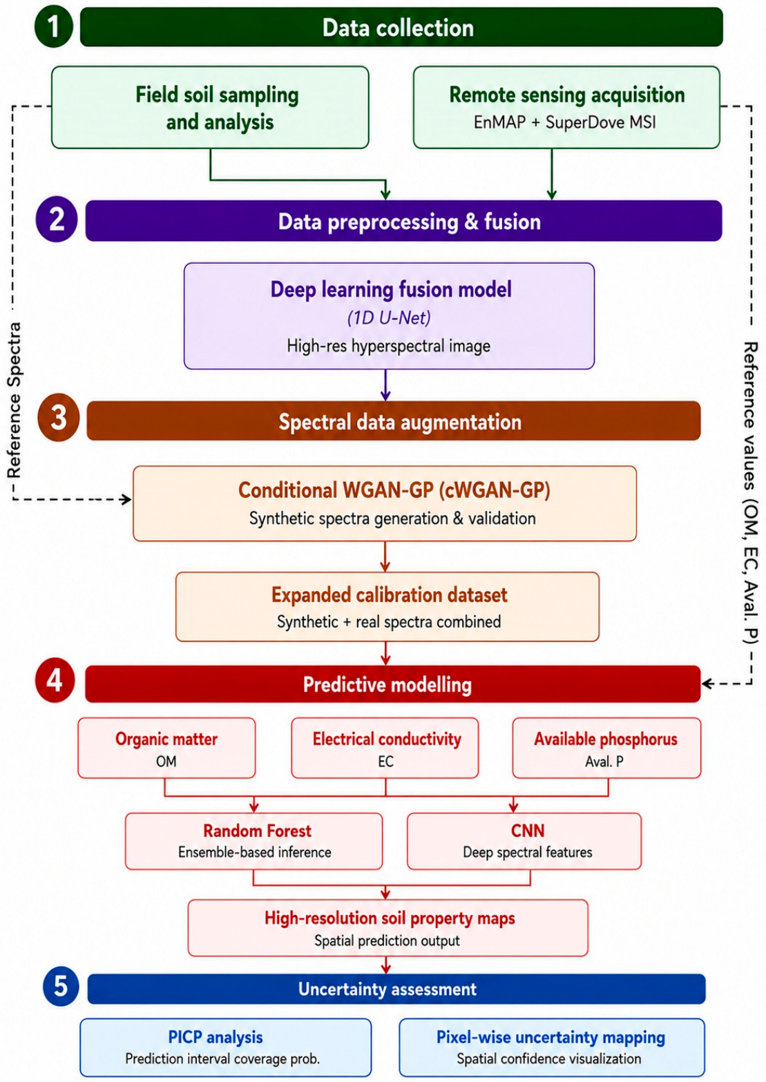
This study employs a comprehensive, multi-stage framework that combines field soil analysis, remote sensing data fusion, spectral augmentation, machine learning and deep learning modelling, and uncertainty assessment to produce high-resolution soil property maps (Figure 1). As part of this framework, the GAN is employed for data augmentation to enhance the diversity of the calibration dataset. The proposed approach integrates generative modelling within a conventional predictive workflow rather than introducing a new predictive model class. In this context, Generative AI refers to the use of generative models to support and enhance conventional predictive modelling approaches rather than replace them [47,48,49,50]. Soil samples were collected and analysed for OM, EC, and P, while remote sensing data were obtained from EnMAP hyperspectral imagery and SuperDove multispectral imagery. These datasets were pre-processed and fused using a deep learning-based fusion model (1D U-Net–CNN) to generate high-resolution hyperspectral data representations. To address limited soil samples, spectral data augmentation was performed using a conditional Wasserstein GAN with gradient penalty (cWGAN-GP), whose output synthetic spectra were validated and matched with real spectra to construct an expanded calibration dataset. Predictive modelling of OM, EC, and P using both the real and synthetic spectra was conducted using random forest (RF) and convolutional neural network (CNN) models. Model performance was evaluated through an independent validation set and uncertainty assessment using prediction interval coverage probability (PICP). Finally, very high spatial resolution (3 m) maps of named soil properties were generated, and their reliability was assessed through uncertainty analysis, including pixel-wise uncertainty mapping.

2.1. Study Area

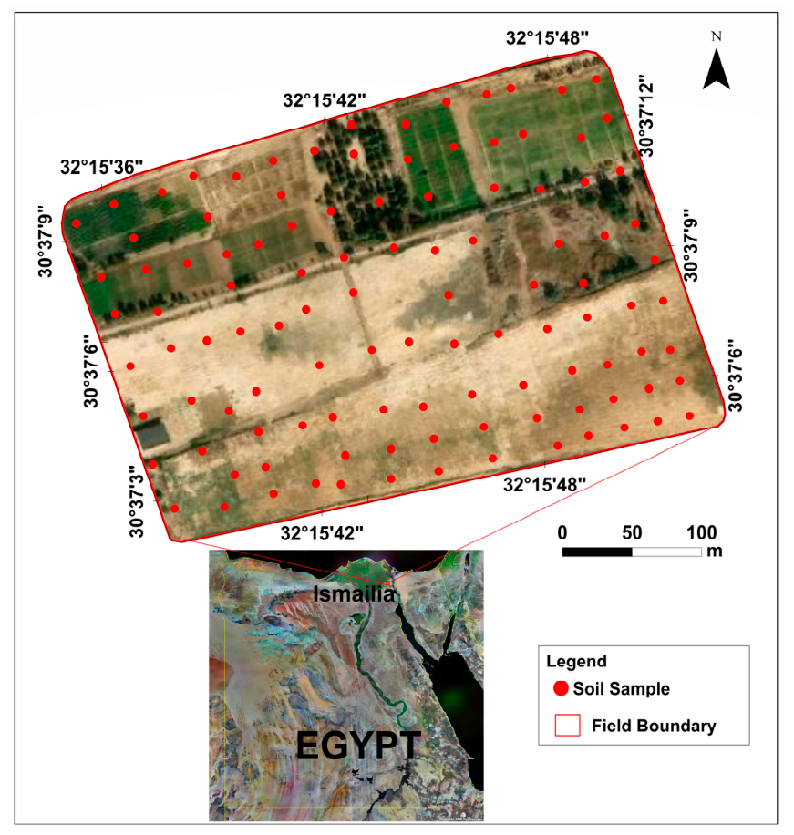
The study area is a five-hectare field located in Ismailia, Egypt (Figure 2). The soil is almost flat, with elevations of 38 to 41 m above sea level. The field is characterised by arid climatic conditions, with hot summers, mild winters, high evaporation rates, and low rainfall intensity (annual precipitation of 22 mm/y). The minimum temperature is recorded in January, while the maximum temperature is recorded in August. The average annual temperature is around 20 °C during the winter months and can reach up to 41 °C in the summer. The soils are derived from alluvial deposits, with dominant textures ranging from sandy loam to loamy sand. According to Soil Taxonomy [51], the soils are classified at the sub-great group level as Typic Torriorthents and Typic Haplocalcids.

2.2. Soil Samples and Analyses

A total of 110 surface soil samples (depth 0–30 cm) were collected on the 16th of September 2024. The study area was characterised by bare soil conditions with negligible vegetation cover at the time of sampling and image acquisition. Around one kg of soil was taken at each location, and the sampling positions were carefully recorded with a global positioning system (GPS) device (Garmin eTrex 10, Garmin Ltd., Olathe, KS, USA). The locations of the samples were selected based on grid sampling to cover the spatial variability of the studied area, accounting for variations in texture and topography as much as possible. The samples were processed carefully by manual removal of the non-soil substances such as grass, roots, stone/gravel, and other non-soil materials. Each fresh soil sample was well mixed, and the sample size was reduced to around 300 g using coning and quartering. The sample was air-dried and sieved to fine earth (<0.002 mm). Soil salinity was determined using electrical conductivity in a soil–water extract 1:2.5 [52]. The soil organic carbon (SOC) was determined by the modified Walkley and Black method [53]. The soil organic matter (OM) was estimated from SOC by applying the Van Bemmelen conversion factor (1.724) [54,55]. Available phosphorus (P) was extracted using 0.5 M NaHCO₃ (at pH 8.5) and determined calorimetrically [56].

2.3. Remote Sensing Data Preprocessing and Fusion

2.3.1. EnMAP Hyperspectral Image

The Environmental Mapping and Analysis Program (EnMAP) provides 224 contiguous spectral bands across the vis-NIR (420–1000 nm) and shortwave infrared (SWIR; 900–2450 nm) regions, with a high spatial resolution of 30 m [57,58]. EnMAP imagery under cloud-free conditions on 18 September 2024 was utilised in this study. The data, processed to Level 2A, offer bottom-of-atmosphere reflectance following atmospheric correction and are ready for quantitative analysis. Spectral regions significantly affected by atmospheric absorption or sensor instability were excluded from the EnMAP spectra before analysis. The removed spectral ranges included 950–1000 nm (VNIR–SWIR overlap region), 1150–1250 nm (weak water vapour absorption), 1400–1450 nm and 1900–2000 nm (strong atmospheric water vapour absorption bands) [19,59]. Additionally, the 1600 and 1680 nm range was excluded due to quality concerns. Consequently, following spectral masking, 178 high-quality spectral bands were retained for further analysis. These pre-processing steps minimized noise propagation into subsequent modelling while preserving important spectral information for analysis.

Soil spectra were extracted from the EnMAP image at the sampling sites with spatial coincidence, resulting in a dataset of 110 soil spectra for model calibration and validation. Precise spectral preprocessing is essential in hyperspectral soil analysis since unprocessed reflectance spectra are often affected by sensor noise, variations in illumination, and scattering effects associated with surface roughness and particle size distribution [60]. Three established preprocessing techniques were used to improve the signal-to-noise ratio and enhance chemically relevant absorption features. First, Savitzky–Golay (SG) smoothing was utilised with a window length of 13 bands and a second-order polynomial to reduce high-frequency noise while maintaining the shape and amplitude of absorption features [61]. Second, standard normal variate (SNV) was applied to each spectrum individually to minimise multiplicative scattering impacts and standardise spectral variability [62]. Finally, a first-derivative SG transformation, employing the same window settings, was used to reduce baseline influences and enhance the absorption features associated with OM and mineral components [63,64]. These preprocessing steps were applied to both the original EnMAP image and the fused image before applying predictive models.

2.3.2. SuperDove (PlanetScope) Multispectral Imagery

SuperDove multispectral imagery with 3 m spectral resolution was used in this study. The SuperDove sensors gather information across eight spectral bands, which include coastal blue, blue, green, yellow, red, red-edge, and two near-infrared bands. The spectral characteristics enhance sensitivity to vegetation state, chlorophyll levels, and soil–vegetation contrast, with the dual near-infrared bands facilitating better differentiation between vegetation structure and soil background influences [65]. The PlanetScope surface reflectance (SR) product was acquired on 19 September 2024 and has been radiometrically calibrated, orthorectified, and atmospherically corrected as surface reflectance with 3 m spatial resolution before being used in data fusion.

For data fusion, the SuperDove image was co-registered to the EnMAP imagery using a common coordinate reference system to ensure spatial consistency. It was then resampled to match the EnMAP spatial resolution and to serve as a high-resolution reference for subsequent downscaling and image-sharpening procedures within the data fusion workflow.

2.3.3. EnMAP–SuperDove Fusion

The EnMAP–SuperDove fusion was designed to exploit the corresponding strengths of hyperspectral and high-resolution multispectral data. The images were projected into a common spatial reference system and accurately co-registered to minimise geometric discrepancies and ensure spatial consistency. Radiometric consistency between the sensors was evaluated, and normalisation procedures were applied where necessary to reduce inter-sensor biases following established multi-sensor harmonisation approaches [66,67]. The resulting integrated dataset facilitated joint spectral–spatial analysis and provided the foundation for subsequent deep learning-based spectral data fusion.

Developing Spectral Data and Preprocessing

The training dataset was constructed by extracting paired spectra from spatially coincident EnMAP and SuperDove imagery at the sampling locations. For each location, the corresponding SuperDove multispectral spectrum and EnMAP hyperspectral spectrum were retrieved through precise spatial matching. The resulting paired dataset comprised SuperDove spectra as model inputs and EnMAP hyperspectral spectra as target outputs. To evaluate model performance, the spectral dataset was randomly divided into a training set (70%, n = 77) and an independent validation set (30%, n = 33). The trained model was then used to reconstruct hyperspectral spectra from SuperDove imagery at 3 m spatial resolution. The resulting product represents a statistically reconstructed hyperspectral image inferred from the learned relationship between SuperDove and EnMAP data.

To ensure methodological consistency across calibration, modelling, and image-scale prediction, all hyperspectral data were harmonised to a common wavelength representation spanning 420–2450 nm. Spectral regions strongly affected by atmospheric water vapour absorption and instrumental noise (950–1000 nm, 1150–1250 nm, 1400–1450 nm, 1600–1680 nm, and 1900–2000 nm) were excluded using a binary wavelength mask. Consequently, the EnMAP spectra were reduced to 178 high-quality spectral bands retained for subsequent analyses. Spectral smoothing was performed using a Savitzky–Golay (SG) filter (window length = 13 bands, polynomial order = 3). In contrast, SuperDove spectra were preprocessed independently using a lighter SG filter (window length = 3 bands, polynomial order = 2) to preserve spectral information while reducing noise. The EnMAP target spectra were standardised using z-score transformation to improve the stability and convergence of the U-Net–CNN model.

Deep Fusion Model for Producing a Hyperspectral High-Resolution Image

A one-dimensional U-Net model was developed to learn the nonlinear relationship between PlanetScope Dove multispectral data and EnMAP hyperspectral data. The 1D U-Net was selected because it effectively learns multi-scale hierarchical representations while preserving fine spectral details. Its encoder–decoder architecture with skip connections captures both local spectral patterns and long-range dependencies while enhancing gradient flow, feature reuse, and spectral consistency, thereby improving the reconstruction of subtle hyperspectral features [68,69]. Previous studies have shown that U-Net-based models consistently outperform conventional CNNs and classical methods in hyperspectral fusion tasks, including pansharpening and super-resolution, due to superior spectral–spatial feature preservation and multi-scale learning [70,71,72]. These characteristics make U-Net architectures well suited for spectral data fusion in remote sensing applications [73]. The model was adapted from the original U-Net framework for biomedical image segmentation [69] and reconfigured for one-dimensional spectral reconstruction. The model operates on spectral vectors of shape (input_dim, 1). The encoder consists of three sequential Conv1D layers with 16, 32, and 64 filters, respectively (kernel size = 3, ReLU activation), each followed by MaxPooling1D for dimensionality reduction while preserving dominant spectral information. The bottleneck layer consists of a Conv1D layer with 128 filters and a kernel size of 5, which learns a compact latent representation that captures the nonlinear relationship between multispectral and hyperspectral domains. This hierarchical design enables the extraction of both fine-scale spectral features and broader spectral patterns. The decoder reconstructs hyperspectral spectra through successive UpSampling1D and Conv1D layers with 64, 32, and 16 filters, respectively. Skip connections concatenate encoder and decoder feature maps, preserving high-resolution spectral information and reducing information loss during downsampling. The final output is generated using a Flatten layer followed by a Dense regression layer, which maps features to the target hyperspectral dimensionality (output_dim) and ensures complete spectral reconstruction.

To justify the selection of the proposed 1D U-Net architecture, a comparative evaluation was conducted using four neural network configurations trained under identical conditions. The reference model was the proposed 1D U-Net, while three alternative architectures were also evaluated: (i) a U-Net without skip connections, (ii) a shallower U-Net with two encoder–decoder levels, and (iii) a conventional CNN consisting of three convolutional layers without an encoder–decoder structure. All models were trained using the same training and validation datasets, optimisation settings, and combined MSE–SAM loss function. Performance was evaluated using R², RMSE, MAE, and spectral angle mapper (SAM), whereas model complexity was assessed based on the number of trainable parameters. This comparison was designed to evaluate the contributions of skip connections, network depth, and the encoder–decoder architecture to spectral fusion performance, thereby providing quantitative justification for the adopted network architecture.

The models were implemented using TensorFlow and Keras in Python. Training was performed using the Adam optimiser with a learning rate of 0.002, 500 epochs, and a batch size of 64. Model optimisation was guided by a composite loss function combining mean squared error (MSE) and SAM. MSE minimises numerical reconstruction error, while SAM preserves spectral shape by constraining angular differences between predicted and reference spectra, which is essential in hyperspectral analysis [74]. To improve robustness and generalisation under limited training data, data augmentation was applied using low-amplitude Gaussian noise and minor spectral shifting, simulating natural variability and reducing overfitting. After training, the model was applied to full PlanetScope Dove imagery to reconstruct an EnMAP-like hyperspectral cube at 3 m spatial resolution. The predicted spectra were inverse-transformed to reflectance space, reshaped into a 3D hyperspectral cube, and exported as georeferenced GeoTIFFs after clipping to the study area for subsequent soil property mapping.

2.4. Spectral Data Augmentation

2.4.1. Spectral Data Generation Using cWGAN-GP and Data Augmentation

A conditional Wasserstein Generative Adversarial Network with gradient penalty (cWGAN-GP) method was used to generate synthetic soil spectra from the calibration spectral dataset extracted from the EnMAP image. The WGAN-GP framework was selected due to its improved training stability and realistic generated hyperspectral data while reducing computational complexity [75,76,77]. The generator of the framework was driven by a 100-dimensional latent noise vector, while the critic was trained with a gradient penalty coefficient of 10 and updated ten times per generator iteration. Model training was conducted for 350 epochs using an adaptive batch size constrained by the calibration sample size. This configuration enforces the Lipschitz continuity condition and reduces mode collapse, which is particularly important for hyperspectral data. The synthetic spectra were generated at multiple augmentation levels (1× to 5× training set), resulting in 77, 154, 231, 308, and 385 spectra, respectively. The generated spectra were validated for dimensional consistency with the real dataset spectra before further analysis.

2.4.2. Matching Synthetic Spectra with Real Spectra and Creating Calibration Datasets

To ensure quality consistency and avoid the inclusion of low-quality synthetic spectra, a principal component analysis (PCA)-based similarity and confidence filtering framework was implemented. The pre-processed real and synthetic spectra were jointly scaled using min–max normalisation and projected into a reduced principal component space comprising five components. For each synthetic spectrum, similarity to the calibration set was quantified using a composite metric that integrates the SAM and Euclidean distance, with weights of 60% and 40%, respectively. Each synthetic spectrum was then assigned to its most similar calibration reference. A two-dimensional PCA representation (PC1–PC2) was subsequently used to define a 90% confidence region based on the chi-square distribution. Synthetic spectra falling outside the confidence region were excluded from further analysis. To evaluate the sensitivity of the filtering procedure, confidence levels of 85%, 90%, and 95% were investigated. As only minor differences in predictive performance were observed among the tested thresholds, a 90% confidence ellipse was selected for subsequent analyses because it provided a balanced compromise between retaining representative synthetic spectra and excluding spectra that deviated from the distribution of the original calibration data. To further control redundancy and mitigate the oversampling effects of synthetic data, a density-based filtering step was subsequently applied. The synthetic spectra were projected into a five-component PCA space, and density-based spatial clustering of applications with noise (DBSCAN) was performed using a small neighbourhood radius (ε = 0.02). Within each cluster, a single representative spectrum was selected based on the minimum Euclidean distance to the cluster centroid in the original spectral space. The resulting filtered synthetic samples from each of the five augmentation levels were combined with the original calibration dataset (n = 77 spectra), which was fully retained without modification, yielding five integrated datasets prepared for the subsequent modelling step.

2.5. Predictive Models for Soil OM, EC and P

The RF model was evaluated alongside the CNN model for predicting OM, EC, and P. The CNN was selected because of its ability to learn hierarchical spectral features and complex nonlinear relationships directly from hyperspectral data. In addition, CNNs can effectively utilise GAN-based data augmentation, which increases the diversity of the calibration dataset and may enhance model robustness and generalisation. Previous studies have also reported that CNN models can achieve performance comparable to, or exceeding, that of conventional machine learning approaches for soil property prediction from spectral data under appropriate conditions [35,36]. Both RF and CNN prediction models were developed using the final combined datasets and evaluated with the independent prediction set for each soil property. The models’ descriptions and development process are provided below.

2.5.1. Random Forest (RF)

RF is an ensemble, non-parametric machine learning algorithm widely used in hyperspectral imaging and DSM. RF can handle high-dimensional, noisy, and correlated predictor variables in hyperspectral imaging [78,79]. The process of RF work is to construct multiple decision trees during calibration. Each tree is trained on a bootstrap sample drawn randomly (with replacement) from the dataset [80]. Randomness is introduced through the bootstrap sampling method and by selecting a random subset of predictor variables at each node split. This decorrelates trees, enhances robustness, and controls multicollinearity, which is a common issue in hyperspectral data [81]. For regression, predictions are obtained by averaging the outputs of all trees, improving generalisation and reducing variance compared to a single decision tree. In this research, RF was used as a benchmark to predict soil properties (OC, EC, P) from pre-processed spectral data. Models were trained with a range of 100–400 trees fitted on augmented calibration datasets (1× to 5×) with fixed random seeds for stability.

2.5.2. Convolutional Neural Network (CNN)

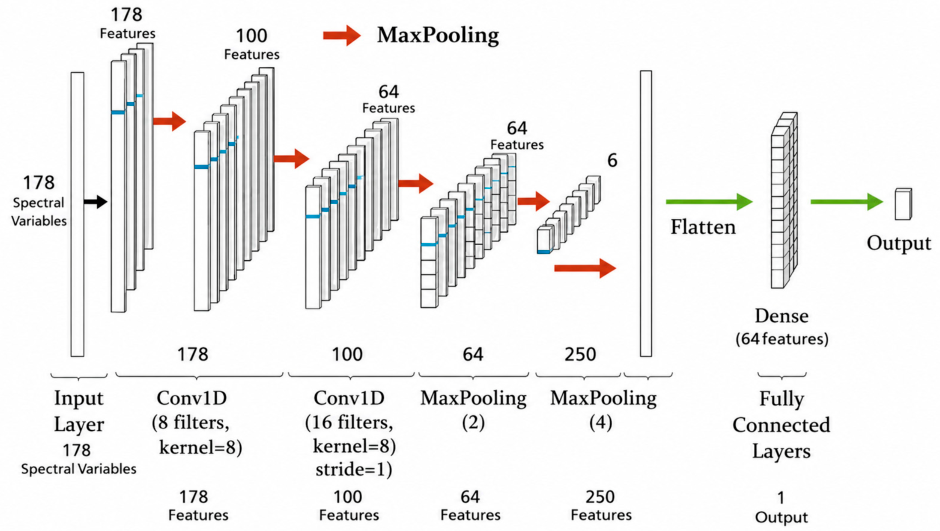
CNNs are deep learning architectures that autonomously extract hierarchical feature representations from structured data [82]. A standard CNN consists of an input layer, convolutional and pooling layers for extracting features and reducing dimensionality, flattening layers to convert features into vectors, fully connected layers, and an output layer. In this research, 1D spectral reflectance data were used as input, maintaining the sequential structure of the spectral information. The original architecture consisted of five convolutional layers, two fully connected layers, and MaxPooling1D layers following each convolution layer to reduce feature dimensionality. Convolutional layers employed ReLU activations, whereas the output layer utilised linear activation for regression purposes. During training, batch sizes ranging from 45 to 64 and 250–500 training epochs were evaluated. To reduce overfitting and improve model performance, batch normalisation, dropout regularisation, and early stopping (patience = 50 epochs) were implemented. The Adam optimiser was used with an initial learning rate of 0.002, which was reduced by 50% when the validation loss failed to improve for 10 consecutive epochs [83]. Batch normalisation and dropout layers were employed to enhance training stability and model generalisation [84].

Following hyperparameter optimisation, a compact seven-layer CNN architecture was developed (Figure 3). The model consists of an input layer containing 178 spectral variables, followed by three convolutional layers with 8, 16, and 32 filters, respectively, using a kernel size of 8 and a stride of 1. Two max-pooling layers with pooling factors of 2 and 4 progressively reduce the feature dimensions, followed by a flatten layer and a fully connected layer before the final regression output. The batch size (49–53) and learning rate (0.001–0.003) were optimised experimentally, while the number of training epochs was determined based on the minimum validation loss. The final architecture contained approximately 20,770 trainable parameters, indicating a computationally efficient and lightweight deep learning model capable of learning complex spectral–soil relationships while minimising the risk of overfitting [85].

2.5.3. Models’ Accuracy Assessment

The RF, GAN–RF, and GAN–CNN models were evaluated using a calibration–validation approach. First, the dataset was randomly divided into calibration (70%) and independent validation (30%) subsets while preserving the correspondence between the soil property measurements and their associated hyperspectral data. The validation subset was kept fixed throughout the study to ensure a fair comparison of the proposed data augmentation framework across all augmentation scenarios. Model development and hyperparameter optimisation were performed using the calibration subset with 10 repeated 5-fold cross-validation (50 models). The optimal hyperparameters were selected based on the lowest cross-validation root mean square error (RMSE_CV). Using these fixed hyperparameters, model performance was then assessed from the mean ± standard deviation of the coefficient of determination (R²), root mean square error (RMSE), and ratio of performance to deviation (RPD) obtained across the 50 cross-validation models. Finally, the optimised models were evaluated using the independent validation dataset. Model performance was quantified using the following metrics:

$$R^2=1- {\displaystyle \frac{{\displaystyle {\sum }_i^n}{\left(x_i-y_i\right)}^2}{{\displaystyle {\sum }_i^n}{\left(x_i-\overline{x}\right)}^2}}$$

(1)

$$RMSE=\sqrt{{\displaystyle \frac{1}{n}}{\sum }_i^n{(x_i-y_i)}^2}$$

(2)

$$RPD={\displaystyle \frac{std}{RMSE}}$$

(3)

where n is the number of samples, xi and yi are measured and predicted values for sample i. $\overline{x}$ is the mean of the measured values, and std is the standard deviation of the measured values. Model performance was evaluated using R², RMSE, and RPD, where higher R² and RPD values and lower RMSE values indicate better predictive performance. Model performance is categorised based on RPD values into six levels [64]: excellent (RPD > 2.5), very good (2.0–2.5), good (1.8–2.0), fair (1.4–1.8), poor (1.0–1.4), and very poor (RPD < 1.0). RF, GAN–RF, and GAN–CNN were implemented in Python 3.8.1 using Keras with TensorFlow backend [86,87].

2.6. Soil Mapping

The fused hyperspectral–high-resolution image was first subjected to the same spectral preprocessing steps applied during model calibration. These steps include first Savitzky–Golay smoothing to reduce noise and enhance spectral features, followed by standard normal variate (SNV) to correct for scatter effects, and finally first derivative transformation to emphasise subtle spectral absorption features relevant to soil constituents. These standardised pixel-wise spectral profiles were then used as inputs to an optimised GAN-CNN model for the prediction of EC, OM, and P. Then, the predictions generated by the CNN models were reconstructed into continuous spatial surface maps by assigning a predicted soil property value to each pixel in the fused image, thereby producing high-resolution maps of EC, OM, and P properties. To facilitate interpretation, the continuous maps were classified into five geometrically spaced classes. Spatial coherence of the maps was improved by applying gap-filling procedures to interpolate missing or noisy pixel values, enhancing the continuity of the spatial surfaces based on reconstructed high-resolution data [88,89]. Post-classification spatial filtering (majority filter) was then applied to suppress isolated anomalies and reduce noise, resulting in smoother and more geographically consistent soil property patterns [90,91]. The robustness of these maps was assessed by comparing predicted values at independent validation locations with values extracted from the continuous maps, ensuring consistency between point observations and spatial predictions as a standard practice in hyperspectral soil mapping validation.

2.7. Uncertainty Assessment

Uncertainty of the models’ predictions and mapping of soil properties (OM, EC, and P) were assessed using a combined framework integrating prediction interval coverage probability (PICP) and pixel-wise uncertainty mapping. The method allows a comprehensive assessment of prediction reliability alongside a spatially detailed illustration of uncertainty, which is crucial to explore the inherited varied performance across different locations. This uncertainty assessment framework has become common in DSM studies that use limited field observations coupled with deep learning models and hyperspectral data, as it enables the modelling of complex relationships between spectral variability and spatial heterogeneity [92].

2.7.1. Prediction Interval Coverage Probability (PICP)

The predicted values of OM, EC, and P were derived using the validation dataset in combination with a bootstrapping approach (100 iterations) to estimate the mean and standard deviation (SD) of the predictions. Based on these statistics, a 90% prediction interval was constructed as mean ± 1.64 × SD [87,93]. The reliability of the uncertainty estimates was subsequently evaluated by computing the prediction interval coverage probability (PICP), defined as the proportion of observed soil measurements falling within the corresponding prediction intervals.

2.7.2. Pixel-Wise Uncertainty Mapping

In addition to the model assessment provided by PICP, spatial variability in prediction reliability was quantified using a pixel-wise uncertainty mapping approach. Prediction residuals were first calculated at validation sample locations as the difference between predicted and observed values. These residuals were then squared and transferred to the raster grid, followed by spatial generalisation using a Gaussian smoothing function. The square root of the smoothed residuals was subsequently computed to derive a continuous uncertainty surface representing the local standard deviation [94,95,96]. This pixel-wise uncertainty map enables the identification of areas with varying prediction reliability, where higher values indicate greater uncertainty. Such spatially explicit uncertainty assessment is particularly important in hyperspectral soil mapping due to the inherent variability in spectral responses and the heterogeneity of soil samples [95].

3. Results

3.1. Soil Analysis and Spectral Data

Table 1. Descriptive statistics of the calibration (Cal) and validation (Val) datasets of soil organic matter (OM), electrical conductivity (EC), and available phosphorus (P).

Property	Dataset	No	Min.	Max.	Mean	Q1	Med	Q3	SD
OM (g kg−1)	Cal	77	6.60	14.30	10.16	8.90	10.10	11.40	1.71
	Val	33	6.80	14.00	9.83	8.60	9.50	11.00	1.61
EC (dS m−1)	Cal	77	0.75	2.50	1.50	1.20	1.48	1.77	0.37
	Val	33	0.70	2.40	1.43	1.18	1.39	1.72	0.36
P (mg kg−1)	Cal	77	8.16	36.16	19.35	16.01	19.46	22.66	5.85
	Val	33	7.76	36.36	20.15	16.46	20.26	24.56	7.14

Note: SD = standard deviation, Q1= first quartile, Q3 = third quartile.

summarises the descriptive statistics of both the calibration (Cal) dataset (n = 77) and the validation (Val) dataset (n = 33) of the tested soil properties (OM, EC, and P). The values of OM in the calibration dataset ranged between 6.60 g kg⁻¹ and 14.30 g kg⁻¹, with a median of 10.10 g kg⁻¹. The first quartile (Q1) and third quartile (Q3) were 8.90 g kg⁻¹ and 11.40 g kg⁻¹, respectively, suggesting a relatively tight distribution and minimal dispersion (SD = 1.71). The validation dataset showed a consistent OM range (6.80–14.00 g kg⁻¹), with slightly lower mean (9.83 g kg⁻¹) and median (9.50 g kg⁻¹) values. The close alignment of calibration and validation statistics indicates an even distribution of OM variability.

EC values in the calibration dataset ranged between 0.75 and 2.50 dS m⁻¹, with an average of 1.50 dS m⁻¹ and a median of 1.48 dS m⁻¹. The interquartile range (IQR) extended from 1.20 dS m⁻¹ for Q1 to 1.77 dS m⁻¹ for Q3, reflecting moderate variability that was confirmed by an SD of 0.37 dS m⁻¹. The validation dataset showed a similar distribution to the calibration set, with values ranging between 0.70 and 2.40 dS m⁻¹ and a slightly lower mean (1.43 dS m⁻¹) and median (1.39 dS m⁻¹). The comparable quartiles and SD (0.36 dS m⁻¹) indicate that the validation set effectively represents the EC variability in the calibration data.

P exhibited the widest variability among the examined properties. The P concentrations of the calibration dataset ranged between 7.20 and 39.20 mg kg⁻¹, with a mean value of 19.97 mg kg⁻¹ and a median of 19.3 mg kg⁻¹. The values of Q1 (15.9 mg kg⁻¹) and Q3 (23.9 mg kg⁻¹), along with a high SD of 6.79 mg kg⁻¹, suggest significant spatial variability. The validation dataset showed a narrow P range (6.80–30.30 mg kg⁻¹) and less variability (SD = 5.22 mg kg⁻¹), while also retaining similar central tendency values, as the mean (16.80 mg kg⁻¹) and median (17.5 mg kg⁻¹) are comparable.

3.2. Quality of Real (Measured) and Synthetic Spectral Data

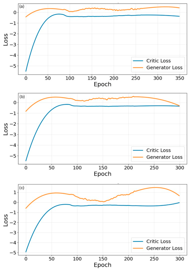
Figure 4 illustrates the changes in generator and critic losses during cWGAN-GP training for producing synthetic spectra for the three soil properties OM, EC, and P. In the initial phases of training, the critic loss shows significant negative values, reflecting a strong ability to differentiate between real and generated spectra. As training advances, the critic loss gradually approaches zero, reflecting a reduction in the Wasserstein distance between real and synthetic spectral distributions. For OM (Figure 4a), the critic loss increases rapidly from highly negative values in the early training stages and levels off close to zero after around 80–100 epochs. After the initial stabilisation phase, the critic loss stays nearly constant with only minor fluctuations. In the meantime, the generator loss gradually increases and follows a smooth trend with minor fluctuations. This behaviour suggests a stable adversarial training process, quick convergence, and a balance interaction between the generator and the critic. The training of EC spectra shows a more gradual and prolonged convergence pattern (Figure 4b). The critic loss gradually rises toward zero and remains stable throughout the training. The generator loss varies slightly around zero, indicating instability. Compared with OM, EC displays a slower convergence process and more persistent training dynamics. For P spectra (Figure 4c), the critic loss shows a similar early convergence pattern but exhibits greater variability during later epochs. The generator loss increases to positive values and shows greater variability compared with OM and EC. Despite this sharp variability, the losses remain limited, showing effective convergence in more dynamic adversarial conditions.

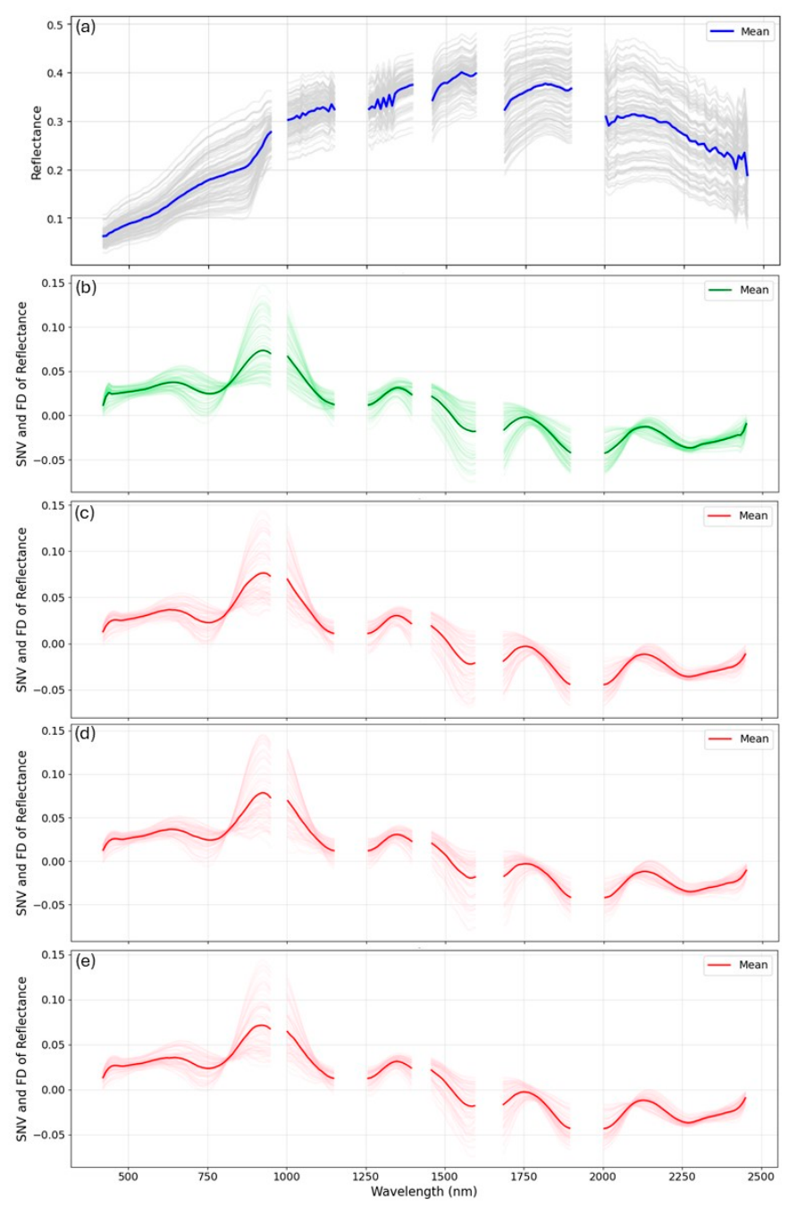
Figure 5 shows the EnMAP soil spectra demonstrating the effect of spectral preprocessing and the agreement between the original and the synthetic spectra. Figure 5a shows the unprocessed EnMAP spectra of the calibration samples, with each spectrum shown as a light blue line and the average spectrum emphasised in bold blue. In the visible range (420–700 nm), reflectance values are generally low and gradually increase with wavelength, a pattern mainly influenced by soil colour, iron oxides, and OM. In the near-infrared region (NIR; 700–1300 nm), reflectance gradually increases, reflecting variations in soil composition and particle size distribution. The absorption features around 1400 nm and 1900 nm, linked to O–H stretching and bending vibrations of water molecules, were eliminated because they are highly noisy, dominated by atmospheric and moisture effects, and provide limited useful information for the analysis. Absorptions in the 1700–1800 nm and 2100–2300 nm regions are associated with organic functional groups (e.g., C–H and C=O bonds) and indicate an indirect relationship to OM content. Furthermore, absorption features around 2200 nm are associated with Al–OH bonds in clay minerals such as kaolinite and illite, whereas features around 2330–2350 nm are typically linked to carbonates and Mg–OH bonds.

Figure 5b illustrates the effect of applying combined standard normal variate and first-derivative (SNV + FD) preprocessing on the EnMAP spectra. This transformation effectively suppresses broad background variation while enhancing localised absorption features. The derivative spectra, with the mean spectrum shown in red, clearly emphasise OM absorption features in the 1700–1800 nm and 2100–2300 nm regions and clay mineralogy absorptions near 2200 nm. Figure 5c–e demonstrates that the cWGAN-GP successfully generates synthetic spectra that closely match the real EnMAP spectra in terms of spectral range, mean spectral shape, and spectral variance across the vis-NIR and SWIR regions. The synthetic spectra occupy the same spectral domain as the processed real spectra and accurately reproduce the main absorption features associated with OM, water hydroxyl groups, and clay minerals. At the same time, the generated spectra exhibit subtle and systematic differences when conditioned on OM, EC, and P values, particularly within OM-sensitive regions (1700–1800 nm and 2100–2300 nm). These properties guide the generative process toward the underlying soil chemical composition, ensuring that synthetic spectra are statistically consistent with observed distributions of OM, EC, and P. Through this conditioning, the model learns to reproduce fine spectral variations linked to these properties, resulting in synthetic spectra that effectively preserve the key characteristics of their corresponding spectral signatures across the spectral domain. Importantly, these controlled variations indicate that the model captures conditions that are dependent on spectral responses rather than introducing random patterns to the generated spectra.

Table 2. Spectral reconstruction performance of four neural network architectures (1D U-Net, U-Net without skip connections, a shallow U-Net with two encoder–decoder levels, and a simple CNN) for EnMAP–SuperDove spectral data fusion.

Model	Trainable Parameters	R2	RMSE	MAE	* SAM
1D U-Net	114,722	0.94	0.0090	0.0060	8.20
U-Net without skip connections	89,282	0.90	0.0097	0.0069	10.87
Shallow U-Net	29,402	0.89	0.0103	0.0078	12.64
Simple CNN	31,250	0.87	0.0111	0.0083	13.53

* SAM = spectral angle mapper.

compares the performance of the four neural network architectures evaluated for hyperspectral spectral reconstruction, including the proposed 1D U-Net, a U-Net without skip connections, a shallower two-level U-Net, and a conventional CNN. The proposed 1D U-Net model achieved the highest reconstruction accuracy, with the highest R² of 0.94, the lowest reconstruction errors (RMSE = 0.009 and MAE = 0.0060), and the smallest spectral angle (SAM = 8.20). Removing the skip connections reduced reconstruction accuracy (R² = 0.90, RMSE = 0.0097, MAE = 0.0069, and SAM = 10.87), indicating that skip connections play an important role in preserving fine spectral information during the decoding process. Likewise, reducing the network depth to a two-level U-Net further degraded performance (R² = 0.89, RMSE = 0.0103, MAE = 0.0078, and SAM = 12.64). The conventional CNN produced the lowest reconstruction accuracy despite having a comparable order of model complexity (R² = 0.87, RMSE = 0.0111, MAE = 0.0083, and SAM = 13.53).

3.3. Spectral Data Augmentation and Developing Calibration Datasets

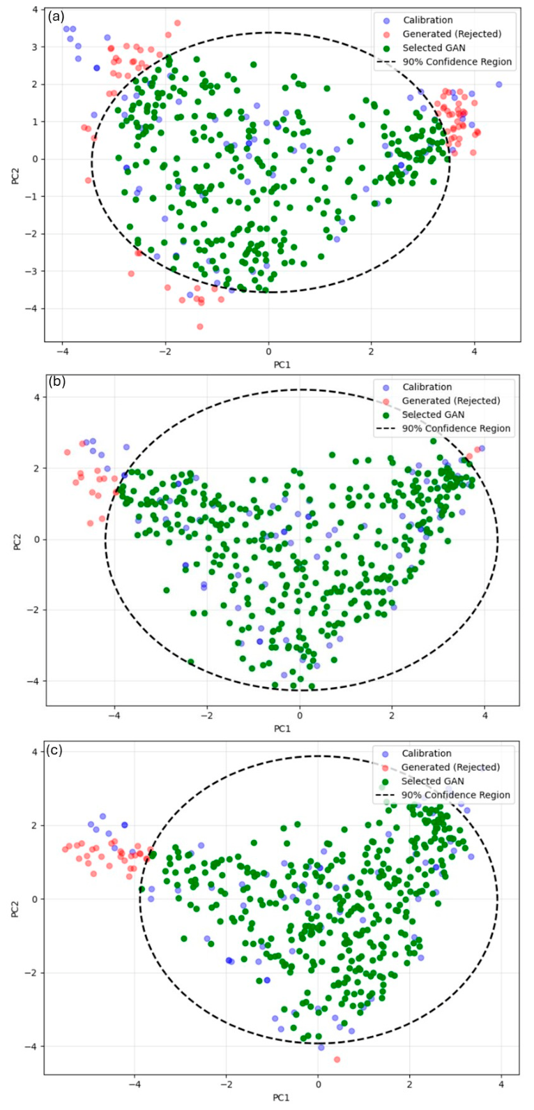
Figure 6 presents the distribution of calibration samples, GAN-generated samples at the different augmentation levels (1×–5×), and the selected subset of GAN samples in the PCA score space (PC1 vs. PC2) for the three soil properties OM, EC, and P. The dashed ellipse denotes the 90% confidence region derived from the calibration dataset for each soil property. Across all properties, the calibration samples (blue points) form a compact and well-defined reference spectral space that captures the inherent field-scale variability of the EnMAP spectral data. In contrast, GAN-generated samples located outside this confidence region (red points) deviate from the statistical structure of the calibration data and were therefore excluded from further analysis. In contrast, the selected GAN samples (green points) show a very close match with the calibration samples, both in terms of spatial distribution and internal structure within the PCA space. These accepted synthetic spectra are located within the 90% confidence region and strongly overlap with the calibration data, indicating a high level of match with the original and synthetic samples. For all soil properties Figure 6a–c), slight variations in point density and distribution are observed. Nevertheless, the relative positioning and overall structure of the calibration and selected synthetic spectra remain consistent. The PCA score (cumulative variance > 90%) represented a significant share of the overall spectral variance across all soil properties, reflecting key spectral information relevant to calibration. The distribution of Mahalanobis distances for the selected GAN-generated samples closely matched that of the original calibration data. More than 90% of the accepted synthetic spectra fell within the 90% confidence limit defined by the calibration covariance matrix. Samples identified as statistically inconsistent were therefore removed before constructing the final calibration dataset. The inclusion of the selected synthetic samples effectively increased the density of the calibration dataset at the 5 levels of augmentation without causing a noticeable shift in the PCA centroid or an increase in spectral variance.

3.4. The Prediction Performance of GAN–RF and GAN–CNN Models

Table 3. Prediction performance of the generative adversarial network–convolutional neural network (GAN–CNN) model trained with combined real and generated spectra at increasing augmentation levels (1×–5×), compared with the GAN–random forest (RF) model. Performance metrics include the coefficient of determination (R²), root mean square error (RMSE), and residual prediction deviation (RPD).

Soil Property				GAN–RF			GAN–CNN
	Generated	Selected	* Cal	R2	RMSE	RPD	R2	RMSE	RPD
OM (g kg−1)	77	62	139	0.69	0.88	1.83	0.76	0.78	2.06
	154	125	202	0.71	0.84	1.90	0.77	0.77	2.10
	231	182	259	0.72	0.84	1.91	0.77	0.76	2.11
	308	241	318	0.71	0.85	1.89	0.73	0.83	1.94
	385	311	388	0.70	0.86	1.85	0.82	0.67	2.38
EC (dSm−1)	77	73	150	0.67	0.20	1.78	0.64	0.21	1.70
	154	146	223	0.67	0.20	1.77	0.76	0.17	2.09
	231	220	297	0.64	0.21	1.69	0.72	0.18	1.95
	308	289	366	0.64	0.21	1.71	0.78	0.16	2.20
	385	368	445	0.64	0.21	1.67	0.85	0.14	2.56
P (mg kg−1)	77	71	148	0.63	3.49	1.69	0.66	3.35	1.76
	154	143	220	0.69	3.18	1.85	0.64	3.49	1.69
	231	215	292	0.68	3.25	1.81	0.67	3.34	1.76
	308	280	357	0.64	3.45	1.70	0.61	3.62	1.63
	385	353	430	0.67	3.31	1.78	0.71	3.15	1.85

* Cal = original calibration samples (n = 77) + the selected generated spectra.

summarises the prediction performance of the GAN–RF and GAN–CNN models for predicting the three soil properties. The models were trained with generated and combined spectra at different augmentation levels (1× to 5×). Model performance was evaluated using R², RMSE, and RPD, while the robustness of these results was further verified using repeated 10 × 5-fold cross-validation. The detailed cross-validation statistics are provided in Appendix A (

Table A1. Mean ± standard deviation of the performance metrics based on repeated 10 × 5-fold cross-validation for the GAN–CNN and GAN–RF models using combined real and generated spectra at increasing augmentation levels (1×–5×). Performance was evaluated using the coefficient of determination (R²), root mean square error (RMSE), and residual prediction deviation (RPD).

				GAN–RF			GAN–CNN
Property	* Gen	* Sel	* Cal	R2	RMSE	RPD	R2	RMSE	RPD
OM (g kg−1)	77	62	139	0.78 ± 0.041	0.72 ± 0.052	2.36 ± 0.17	0.83 ± 0.036	0.60 ± 0.046	2.65 ± 0.19
	154	125	202	0.81 ± 0.038	0.69 ± 0.047	2.46 ± 0.17	0.84 ± 0.033	0.58 ± 0.042	2.76 ± 0.19
	231	182	259	0.83 ± 0.035	0.67 ± 0.045	2.54 ± 0.17	0.87 ± 0.031	0.55 ± 0.040	2.96 ± 0.20
	308	241	318	0.82 ± 0.036	0.68 ± 0.046	2.49 ± 0.17	0.85 ± 0.032	0.57 ± 0.041	2.86 ± 0.19
	385	311	388	0.81 ± 0.034	0.69 ± 0.044	2.45 ± 0.16	0.88 ± 0.029	0.54 ± 0.038	3.05 ± 0.20
EC (dS m−1)	77	73	150	0.74 ± 0.044	0.17 ± 0.017	2.21 ± 0.22	0.81 ± 0.038	0.14 ± 0.015	2.48 ± 0.25
	154	146	223	0.76 ± 0.041	0.16 ± 0.016	2.28 ± 0.22	0.84 ± 0.034	0.13 ± 0.014	2.75 ± 0.28
	231	220	297	0.78 ± 0.039	0.15± 0.015	2.36 ± 0.23	0.86 ± 0.032	0.12 ± 0.013	2.95 ± 0.30
	308	289	366	0.77 ± 0.040	0.160 ± 0.016	2.32 ± 0.23	0.85 ± 0.033	0.13 ± 0.013	2.85 ± 0.29
	385	368	445	0.76 ± 0.038	0.16 ± 0.015	2.26 ± 0.21	0.89 ± 0.029	0.11 ± 0.012	3.29 ± 0.35
P (mg kg−1)	77	71	148	0.72 ± 0.046	2.85 ± 0.214	2.05 ± 0.15	0.78 ± 0.040	2.56 ± 0.187	2.28 ± 0.17
	154	143	220	0.76 ± 0.043	2.67 ± 0.198	2.18 ± 0.16	0.81 ± 0.037	2.42 ± 0.173	2.41 ± 0.17
	231	215	292	0.79 ± 0.040	2.53 ± 0.186	2.31 ± 0.17	0.82 ± 0.035	2.31 ± 0.161	2.45 ± 0.18
	308	280	357	0.78 ± 0.041	2.59 ± 0.191	2.25 ± 0.17	0.83 ± 0.036	2.30 ± 0.166	2.48 ± 0.18
	385	353	430	0.77 ± 0.039	2.64 ± 0.185	2.21 ± 0.15	0.85 ± 0.033	2.18 ± 0.152	2.67 ± 0.19

* Gen = generated, * Sel = selected, * Cal = original calibration samples (n = 77) + the selected generated spectra.

). In general, the CNN model showed a distinct and steady enhancement in predictive performance as the augmentation size grew for the three evaluated soil properties. This trend suggests that adding generated spectra significantly improved the CNN’s capacity to understand the effective connections between spectra and soil properties. For OM, the CNN models consistently surpassed the benchmark RF (without augmentation) at every level of augmentation. The GAN–RF model exhibited consistent performance, with R² values ranging between 0.69 and 0.72 and RPD values ranging from 1.83 to 1.91, reflecting good predictive capability [64]. In comparison, the GAN–CNN model showed a significant enhancement in accuracy, as R² increased from 0.73 to 0.82 at 5× augmentation. As a result, RMSE declined from 0.83 to 0.67 g kg⁻¹, while the RPD value reached a maximum of 2.38 (very good performance). This trend indicates that expanding the calibration set with the selected generated spectra improved the predictive performance of the GAN–CNN model for OM prediction.

A noticeable positive effect of augmentation was also observed for the EC models. The benchmark RF model again showed limited sensitivity to the increased number of selected and combined samples, with R² values of 0.64–0.67 and RPD values below 1.80, suggesting fair but not robust predictions (Table 3). The GAN–CNN model gained advantages from data augmentation. Although its performance with 1× augmentation was comparable to GAN–RF (R² = 0.64, RPD = 1.70), significant improvement was obtained with the largest augmentation sizes. With 5× augmentation, GAN–CNN achieved the best results with R² of 0.85, RMSE of 0.14 dSm⁻¹, and RPD of 2.56. These results confirmed that the CNN model successfully utilised the generated spectra to manage non-linear relationships that GAN–RF did not thoroughly investigate.

The P model’s prediction performance was lower than that of the OM and EC models (Table 3). The GAN–RF model showed fair to good prediction with R² (0.63–0.69) and RPD (1.69–1.85) that was better than the benchmark RF model. The GAN–CNN model showed the same trend as the OM and EC models, with notable improvement results observed compared with the benchmark RF model at 5× augmentation. The model achieved fair to good predictive performance, with R² increased from 0.64 to 0.71, RMSE decreased from 3.48 to 3.15 mg kg⁻¹, and RPD improved from 1.67 to 1.85. These findings suggest that increasing the augmentation size positively enhanced the predictive performance of the P models, although the prediction accuracy remained lower than that achieved for OM and EC.

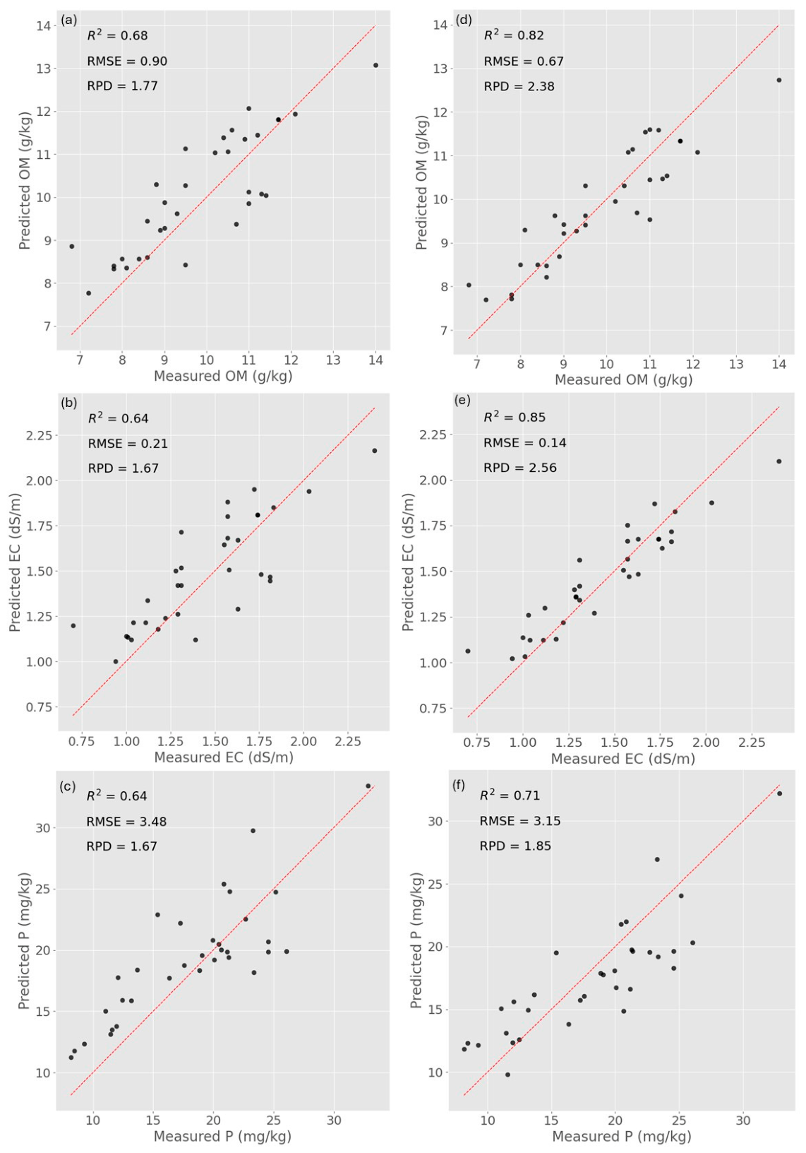
Figure 7 illustrates the best results of GAN–CNN models based on the optimal datasets for predicting OM, EC and P compared with the results of the RF benchmark models. The results demonstrated that the GAN–CNN models always outperformed the RF models across all soil properties, indicating the positive effect of data augmentation on prediction performance, as higher values of R² and RPD, and lower RMSE were calculated. For OM, the GAN–CNN model trained on 384 combined samples achieved the best result with R² of 0.82, RMSE of 0.67 g kg⁻¹, and RPD of 2.38, substantially outperforming the RF model (R²= 0.68, RMSE = 0.9 g kg⁻¹, RPD = 1.77). Similarly, for EC, the GAN–CNN model developed based on 445 combined samples resulted in high predictive performance (R² = 0.85, RMSE = 0.14 dSm⁻¹, RPD = 2.56), compared with the RF model (R² = 0.64, RMSE = 0.21 dSm⁻¹, RPD = 1.67). The predictive performance of P models was generally lower than that of OM and EC. However, the GAN–CNN model still showed clear improvement (R² = 0.71, RMSE = 3.15 mg kg⁻¹, and RPD = 1.85) relative to RF (R² = 0.64, RMSE = 3.48 mg kg⁻¹, RPD = 1.67).

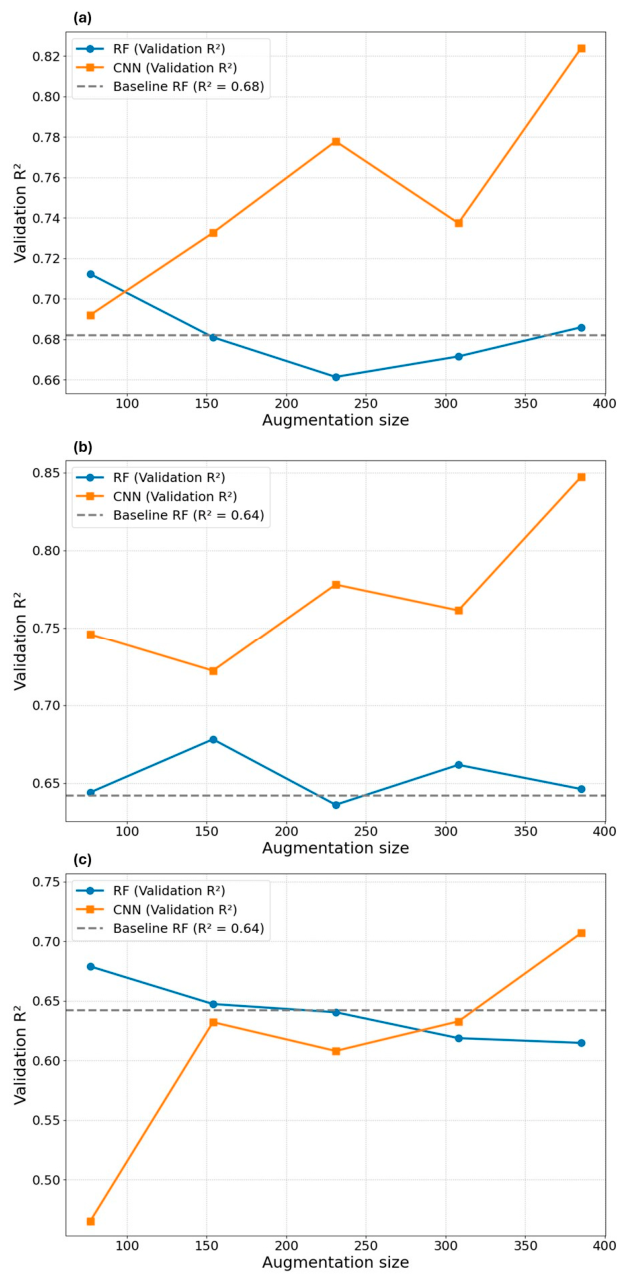
Figure 8 shows the effect of augmentation size on the validation prediction performance, indicated as R² of the GAN–RF and GAN–CNN models for predicting OM, EC, and P. For OM, the CNN model always outperformed the RF model at all augmentation levels. The CNN validation R² gradually increased as more augmented data were added. The best results were achieved with the largest augmentation size (5×). The GAN–CNN model based on the 5× augmentation achieved the best validation results with an R² of 0.82. These results indicate a clear improvement of the CNN model compared with the RF baseline developed without augmentation (dashed line, R² = 0.68). The GAN–RF model showed a notable reduction compared with the baseline performance, suggesting no impact of additional synthetic data. Similarly, the results of EC models indicate that increasing augmentation size improves the performance of GAN–CNN, and the highest results are achieved with R² (0.85) at the 5× augmentation level. The GAN–RF performance remained relatively stable and close to the RF baseline model, with an R² of 0.64, with only small changes across the different augmentation levels. This indicates that the GAN–CNN model was better able to exploit the additional variability introduced by the generated spectra. For P, the response to augmentation was more variable. The GAN–CNN model showed a steady improvement with increasing augmentation size, achieving its best performance at 5× augmentation (R² = 0.71). In contrast, the GAN–RF model demonstrated a consistent decline in performance, indicating an inverse relationship with augmentation level, where performance decreased as augmentation increased.

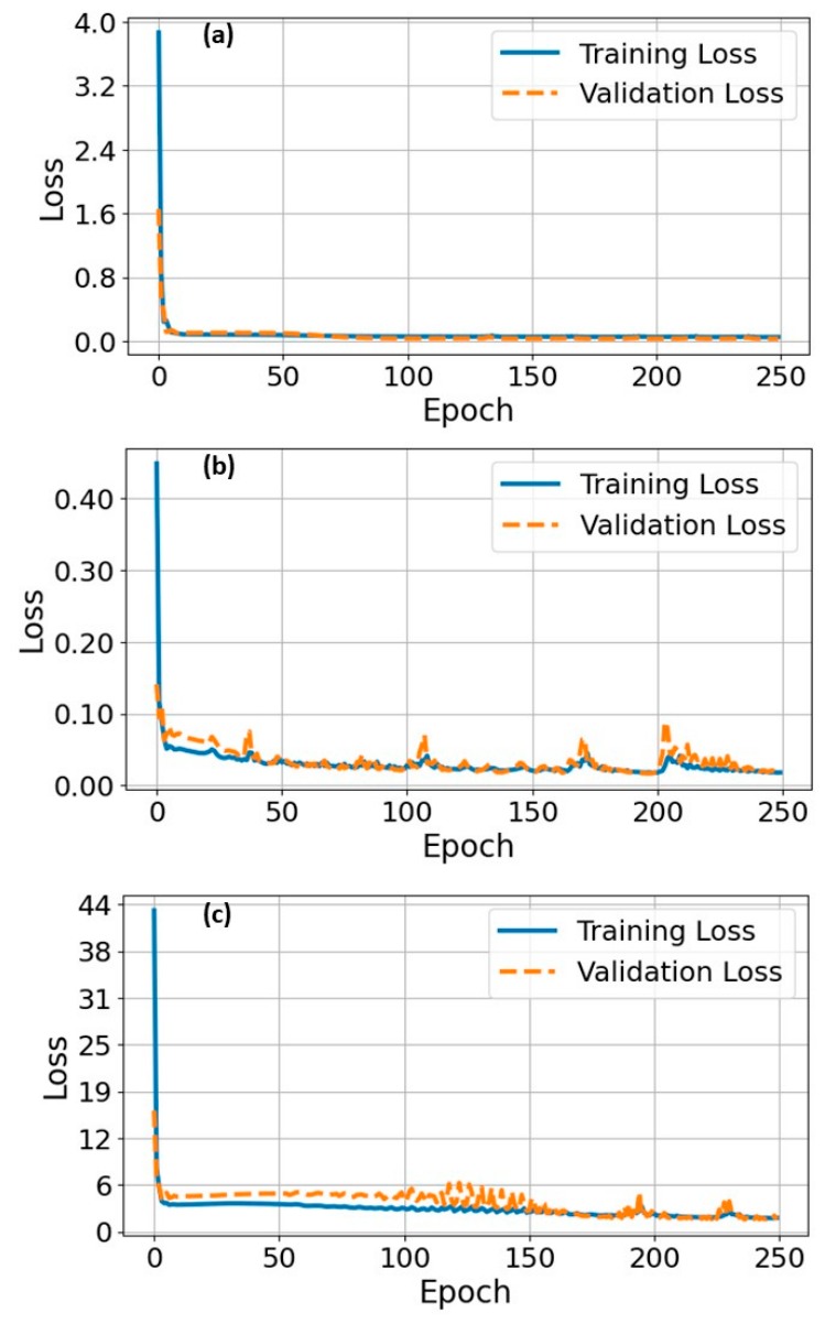
Figure 9 shows the training and validation loss curves for the optimal CNN–GAN models developed for OM, EC, and P. For all three soil properties, both losses decreased rapidly during the early epochs, indicating effective learning of the underlying spectral–soil relationships, followed by a gradual decline and stabilisation, demonstrating model convergence. The OM model (Figure 9a) exhibited a smooth, consistent reduction in both losses, while the EC model (Figure 9b) converged more gradually with minor fluctuations in validation loss. Similarly, the P model (Figure 9c) showed a substantial initial reduction, with training and validation losses remaining closely aligned throughout training. This pattern was consistently observed across all models.

3.5. The Uncertainty of Predictive Models

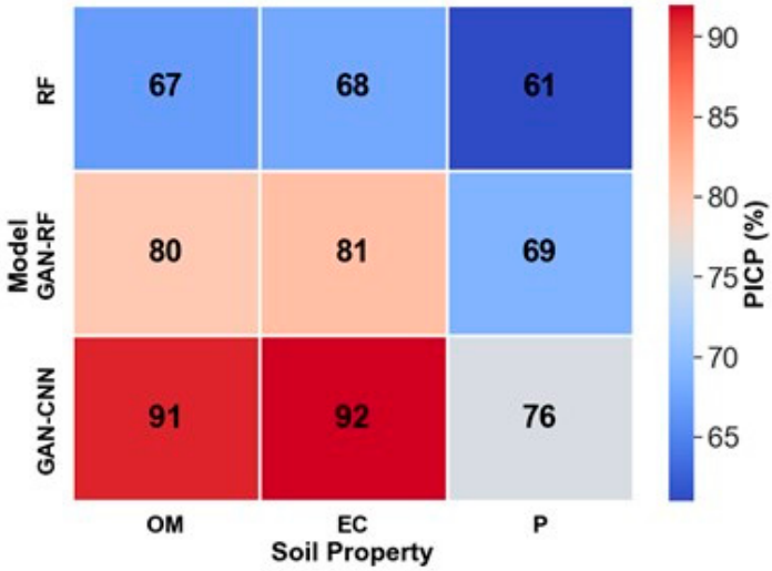
The performance of baseline RF, GAN-RF, and GAN-CNN models for predicting OM, EC and P properties was evaluated using PICP at a 90% confidence level (Figure 10). The PICP values indicated reliable coverage of the predicted intervals. For OM, the baseline RF model captured approximately 67% of true values within its prediction intervals. GAN-based augmentation improved coverage, with GAN-RF achieving 80% and GAN-CNN reaching 91%. Similarly, for EC, the baseline RF model achieved 68% coverage, whereas GAN-RF and GAN-CNN increased PICP to 81% and 92%, respectively. The P predictions were the most challenging for the baseline RF, with a PICP of 61%. GAN-RF and GAN-CNN substantially improved coverage to 69% and 76%, respectively. These results demonstrate that GAN-CNN consistently increased the PICP values for all soil properties, indicating both improved reliability and uncertainty quantification in the predicted soil properties.

3.6. Soil Property Maps and Associated Uncertainty

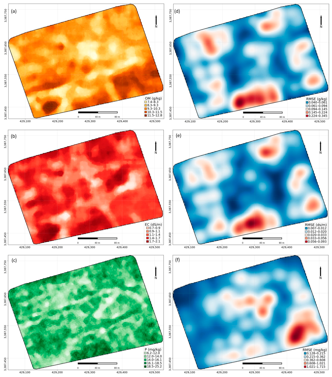
The spatial distribution maps highlight the capability of a hyperspectral–multispectral high-resolution fused image to represent fine spatial variability of the soil properties (Figure 11). The fusion approach effectively transferred hyperspectral information to a finer spatial grid (3 m), enhancing the representation of very detailed soil variability at the field scale. The predicted OM map (Figure 11a) revealed substantial within-field variability, with distinct spatial structures rather than random patterns. The OM content (10.3–11.5 g kg⁻¹) dominated the field with an area of 65.2%, while the highest OM content ranged between 11.5 and 12.8 g kg⁻¹ covered 9% of the field, and it appeared as hotspots. The medium OM value (9.3–10.3 g kg⁻¹) covered 25.4% of the field. While the lowest OM content (7.4–9.3 g kg⁻¹) represents only 0.4% of the field, it appears as scattered areas in uncultivated soils with limited fertility. The pixel-wise uncertainty map was classified into five RMSE classes to quantify the spatial extent of uncertainty. The RMSE map for OM (Figure 11d) showed that low-error areas (0.04–0.09 g kg⁻¹) covered 5.26%. In contrast, high-error areas (0.22–0.34 g kg⁻¹) occupied 14.6%, reflecting a substantial portion of the study area with elevated uncertainty. Moderate uncertainty (0.094–0.022 g kg⁻¹) accounted for approximately 80% of the total area, suggesting generally stable predictions across most of the field.

EC map (Figure 11b) showed relatively smoother and more continuous spatial gradients compared to OM. Although the range of salinity range remined low (0.7–2.1 dS m⁻¹) in the semiarid region, the salinity map revealed pronounced spatial heterogeneity across the field. The majority of the field area (67.1%) was dominated by intermediate EC values, with a range (1.1–1.7 dS m⁻¹). The low salinity (0.7–1.1 dS m⁻¹) accounted for 0.9% of the field. The highest salinity range (1.7–2.1 dS m⁻¹) covered 32% of the field. The RMSE-based uncertainty map (Figure 11e) indicated that areas with the lowest prediction errors (0.007–0.02) covered 17.2% of the field’s total area, reflecting zones of high model reliability. In contrast, the highest-error areas (0.05–0.09) covered 18.1%, highlighting localised regions where predictions are less certain. The majority of the field (64.7%) was dominated by moderate uncertainty (0.02–0.05), suggesting that predictions are generally stable across most locations.

The predicted P map (Figure 11c) displayed notable spatial variability across the field, with five classes ranging from 10.8 to 22 mg kg⁻¹. Generally, spatial distribution reveals low content of P across the field. Most of the field area was dominated by moderate P levels ranging from 14.0 to 18.54 mg kg⁻¹, covering 44.6% of the area, forming broad and continuous zones indicative of relatively uniform fertility. Lower P values (6.2–11.9 mg kg⁻¹) were less extensive, covering 13.8% of the field. In contrast, the highest P values (18.5–25.1 mg kg⁻¹) covered the smallest area of 13.7%. The RMSE-based uncertainty map for P (Figure 11f) indicated that areas with the lowest prediction errors (0.12–0.21) covered 4.7%, representing regions of high model reliability. High-error areas (1.02–1.71 mg kg⁻¹) covered 18.2% of the field area, highlighting localised zones where predictions are less certain. Most of the field area was dominated by moderate uncertainty (0.21–1.02 mg kg⁻¹), which covered 77.1% of the area. This distribution demonstrates a controlled uncertainty pattern, with moderate errors prevailing and extreme errors limited.

4. Discussion

4.1. EnMAP and Synthetic Spectral Data Quality

The spectral reflectance patterns in the EnMAP spectrum align with the principles of vis-NIR spectroscopy. The vis–NIR spectrum is affected by the moderate to high levels of OM content [60]. The detected absorption features in the ranges of 1977–2059 nm, 2182–2232 nm, and >2300 nm relate to overtones and combination bands of O–H, C–H, and N–H bonds, linked directly to interactions between OM and clay minerals [60,97]. In the visible range, features between 460 and 582 nm were important, indicating the effect of soil iron oxides and organic coatings on reflectance, aligning with findings in the literature [60,98,99]. Wavelengths ranging from 1570 to 1630 nm were also essential, corresponding with earlier research indicating that these regions identify the OM absorption feature with limited soil moisture interference [100]. EC and P showed less distant spectral features because of their indirect spectral responses. EC indicates soluble salts and moisture levels, resulting in wide, nuanced spectral changes instead of distinct absorption peaks [101]. For P, there is no direct spectral response, and its predictive potential is mainly related to the relationship with OM, clay composition, and carbonate minerals [60,100]. This clarifies the comparatively lower R² for P compared with OM and EC, a finding which aligns with results reported in earlier hyperspectral soil research [102,103].

In this study, the cWGAN-GP successfully produced synthetic soil spectra that matched the real spectra in both shape and characteristics. This indicates the ability of the cWGAN-GP to capture the inherent soil spectral patterns, providing an improvement in hyperspectral data augmentation with a limited real sample. The conventional GANs based on Jensen–Shannon divergence often suffer from unstable training and mode collapse, which limit their ability to represent the continuous variability of spectral reflectance [104,105]. The Wasserstein GAN (WGAN) framework improves training stability by optimising the Wasserstein distance between real and generated data distributions [106]. But WGAN may result in unstable optimisation and reduced sample quality as it enforces the Lipschitz constraint through weight clipping. The WGAN-GP approach replaces weight clipping with a gradient penalty applied to the critic’s gradients with respect to its inputs, providing more stable training and improved convergence [75]. The cWGAN-GP use the Wasserstein-1 distance to create a smooth and informative learning spectral space even between small, diverse real spectra and synthetic spectra [107,108]. This method generates spectrally consistent samples that better reflect the statistical distribution of real hyperspectral data, supporting more robust predictive modelling in remote sensing applications [109,110]. The proposed framework can generate plausible spectral representations for indirectly inferred soil properties, such as phosphorus (P), which lacks distinct absorption features in the Vis–NIR region and is instead estimated through multivariate relationships with spectrally active soil components [60,64]. Although the generated spectra closely matched the distribution of the measured data, preserving the overall spectral distribution does not necessarily ensure that the covariance structure underlying these indirect relationships is fully maintained. As a result, subtle spectral artifacts affecting indirectly inferred properties cannot be completely ruled out, and representation quality may be lower for P than for spectrally responsive properties such as EC and OM [60]. Future studies should further evaluate whether GAN-generated spectra preserve the physicochemical relationships between spectral responses and soil properties, particularly for indirectly inferred attributes such as phosphorus, through dedicated spectral artifact analyses. Despite this limitation, the proposed framework has considerable potential for hyperspectral imaging applications, where reflectance signatures are highly sensitive to variations in moisture, mineral composition, and OM [110,111].

This study established a quality control framework for synthetic spectra. The framework leveraging PCA–Mahalanobis distance filtering ensures reliability through the projection of both real and generated spectra into PC space and evaluating their Mahalanobis distances. This method is conceptually similar to the recently suggested “Teacher–Student” reliability validation technique utilised in spectral mapping studies of soil salinity [41]. This filtering approach ensures accurate selection of only high-quality synthetic spectra with robust correlations with original spectra, while maintaining critical diagnostic absorption features linked to soil chemical composition [36,112]. In the current research, results showed a promising capability of cWGAN-GP to efficiently expand the spectral dataset and address the challenge of a limited dataset in hyperspectral imaging. Recently, salinity modelling and mapping have been improved by expanding 110 soil samples with 1100 reliable synthetic spectra using generative techniques [41]. This is because using a generative method enhances spectral datasets and bridges the gaps to develop a more robust basis for hyperspectral analysis and mapping with limited samples [35]. It was reported that generative spectral augmentation has significantly improved OC prediction in hyperspectral datasets. For example, Jiang et al. [110] reported that adding generated spectra from GAN to the calibration set of the CNN model increased the R² by approximately 4.6% and reduced RMSE by 18.96% compared with the CNN models trained only on real spectra. Similarly, Xia et al. [113] demonstrated that a doubly regularised WGAN-GP combined with a CNN model improved SOC prediction in tobacco fields with increased R² from 0.76 to 0.86 and decreased RMSE from 3.48 to 2.64 mg kg⁻¹. These findings suggested that high-quality synthetic soil spectra not only augment constrained datasets but also improve the accuracy and generalisation of models in hyperspectral analysis.

4.2. Effect of Data Augmentation on Model Accuracy and Uncertainty

The performance of deep learning models depends on the availability of sufficiently large and representative training datasets, which remains a major challenge in hyperspectral soil analysis. Limited sample sizes increase the risk of overfitting and reduce model generalizability, particularly for high-capacity architectures such as CNNs and GANs [110,114]. This challenge is further compounded by the high dimensionality and collinearity of hyperspectral data, which increase sensitivity to sampling variability and may lead to site-specific rather than transferable spectral–soil relationships [35]. To mitigate these limitations, a cWGAN-GP-based augmentation strategy was employed to expand the calibration dataset approximately five-fold (from 77 to 385 samples), thereby increasing the diversity of spectral patterns available during training. The augmented dataset was combined with dropout regularisation and early stopping to reduce overfitting and improve model generalisation. Previous studies have demonstrated that GAN-based augmentation can substantially enhance CNN performance under limited-data conditions, including soil spectroscopy applications with as few as 42 samples [110], while the combined use of data augmentation and regularisation has been shown to improve model stability and predictive performance in data-constrained scenarios [110,115,116]. Nevertheless, synthetic spectra should be regarded as complementary to, rather than replacements for, real observations. The effectiveness of generative augmentation ultimately depends on the quality and representativeness of the original dataset. Therefore, larger and more diverse field datasets remain essential for improving model robustness, generalizability, and transferability across diverse soil types and environmental conditions.

Despite these limitations, the results suggest that integrating deep generative AI with hyperspectral data can enhance CNN performance under data-constrained conditions. The cWGAN-GP augmentation strategy increased spectral diversity and contributed to improved prediction of OM, EC, and P. These findings are consistent with previous studies reporting that generative augmentation can better preserve the underlying structure of spectral data than conventional augmentation approaches [35]. Furthermore, CNNs appeared to benefit more from spectral data augmentation than RF models, which depend on ensemble decision boundaries instead of continuous spectral feature learning [80]. Expanded spectral datasets may therefore enable CNNs to better capture meaningful relationships between soil reflectance and soil properties [117,118]. In contrast, CNN models without data augmentation tend to focus on spectral noise rather than learning meaningful chemical relationships between soil reflectance and measured properties [44,119]. Consequently, CNN models without data augmentation may suffer from compromised accuracy and constrained robustness in hyperspectral analysis [117,120]. The CNN–GAN framework demonstrated stable optimisation and effective learning of nonlinear spectral–soil relationships. The close agreement between the training and validation loss curves throughout the training process indicates limited overfitting and good generalisation ability. The minor fluctuations in the validation loss for EC and P models may be attributed to their relatively weak and indirect spectral response. These results are consistent with previous studies showing that GAN-based spectral augmentation enhances data diversity, improves model performance, and promotes stable model training in soil property prediction [41,121], further supporting the effectiveness of integrating CNN feature learning with GAN-based augmentation.

The OM results obtained using the GAN–CNN model demonstrated consistent improvements compared to the RF modelling. The results confirm that generative augmentation can effectively capture complex spectral variability related to OM and enhance predictive performance. At the highest level of augmentation, R² increased by 25.6% while RMSE decreased by 22.2%, indicating a substantial gain in model accuracy. This improvement suggests that augmenting the spectral dataset enhances the representation of nonlinear OM spectral relationships, which are often underrepresented in limited spectral datasets. These results are in agreement with a recent study that reported CNN models trained on augmented datasets outperformed RF in predicting SOC [120]. The authors used a hybrid framework combining a conditional variational autoencoder with a convolutional neural network (CVAE–CNN) to generate SOC-conditioned spectra and overcome data scarcity in estimating SOC based on NIR spectra [120]. The improved performance can be attributed to the ability of augmented datasets to increase spectral diversity and enable deep learning models to better learn nonlinear relationships [120,122]. Importantly, the generated spectra can be interpreted as probabilistic interpolations within the OM chemical continuum rather than simple replications of observed samples [44,46]. This enables the synthetic data to introduce continuous OM values while preserving the underlying feature space, thereby capturing natural soil gradients and enhancing model generalisation [46]. This is consistent with previous studies demonstrating that increasing the size and diversity of spectral datasets enhances the accuracy of OM prediction [119,120]. Moreover, GAN-generated spectra have been shown to improve regression stability by effectively preserving the inherent reflectance distributions [44,122]. Nevertheless, careful validation using independent datasets at different regions remains essential to ensure the reliability and transferability of the GAN–CNN models, as the quality of synthetic spectra depends strongly on the representativeness and size of the original training dataset.

A similar improvement was observed in EC prediction using the GAN–CNN model, where spectral data augmentation significantly enhanced predictive performance. Specifically, R² increased by 31.3%, and RMSEP decreased by 33.2% after 385 synthetic samples were incorporated into the calibration dataset. These results suggest that data augmentation effectively enhances the representation of spectral variability associated with soil salinity levels, particularly under conditions of limited sample availability. CNNs are well-suited for hyperspectral analysis, as they can capture local spectral patterns and dependencies across adjacent wavelengths, allowing them to detect subtle spectral variations linked to complex scattering behaviours [120,122]. Moreover, the cWGAN-GP approach can generate realistic synthetic spectra that enhance model robustness and generalisation through improved feature learning [117]. These results are consistent with recent hyperspectral generative modelling research demonstrating that Wasserstein-based GAN architectures improve salinity modelling reliability under environmental variability conditions [41]. This is particularly important, as soil salinity signatures are governed primarily by indirect scattering effects, surface salt crystallisation, and moisture–salt interactions rather than distinct absorption features [41,101]. Consequently, salinity prediction is highly sensitive to dataset sparsity and spectral heterogeneity, further emphasising the importance of spectral data augmentation.

As expected, the prediction performance of all P models was lower than that of the OM and EC models. Indeed, accurate prediction of P using NIR spectral data remains difficult because of its weak and indirect spectral signature. P lacks distinct diagnostic absorption features in the vis–NIR region and is therefore estimated indirectly through its associations with spectrally active soil components, including iron oxides, clay minerals, and organic matter [60,87]. Therefore, the response of P is often masked by stronger spectral responses from the dominant mineral, making robust prediction difficult. However, in this study, the predictive performance improved substantially after applying spectral data augmentation. The R² increased by 9%, while RMSEP decreased by 8.2%, reaching an optimal prediction of R² = 0.71 and RMSEP = 3.15 mg kg⁻¹ following the addition of 385 generated spectra. These results are in line with those reported by recent research on estimating soil properties based on indirect spectral responses [110,123,124]. Specifically, Vullaganti et al. [124] observed an increase in prediction accuracy with R² values increasing from 0.44 to 0.68 when using spectral data augmentation. Furthermore, Jiang et al. [110] demonstrated that GAN-generated spectral augmentation (15–240 samples) improved CNN-based P prediction with an 8.3% increase in R² and a 35.7% reduction in RMSEP. These findings highlight the role of augmentation in capturing nonlinear hyperspectral–soil relationships [125,126]. Consequently, CNN with data augmentation resulted in performance enhancements of 33–42% in predicting soil properties, including P [126]. This improvement can be attributed to the ability of generative augmentation to expand the spectral feature space while maintaining consistency with target nutrient values. As a result, the synthetic samples preserve the statistical characteristics of real spectra and follow the underlying soil spectral distribution [120,122]. This expansion of the dataset enables models to better capture indirect spectral variations associated with P and soil properties interactions [110,124]. The PICP analysis reveals significant improvements in model predictions through spectral data augmentation. The baseline RF model demonstrated substantial under-coverage with PICP values (61–68%), indicating that traditional ML models trained on limited datasets produce overly narrow prediction intervals. Such under-coverage reflects a common limitation where conventional uncertainty estimation methods fail to adequately capture the true variability in soil spectral data [127]. The incorporation of GAN-based data augmentation substantially improved PICP performance, with the GAN-RF models (69–81% coverage). This improvement demonstrates that enhanced dataset diversity through synthetic data generation enables models to better approximate the true data distribution and provide more realistic uncertainty estimates. The benefits of data augmentation are supported by findings of Liu et al. [128], who showed that spectral data fusion techniques significantly enhanced prediction accuracy of key soil properties including SOM, total nitrogen (TN), and available potassium (AK) with R² improvements ranging from 0.06 to 0.41, indicating that increased data diversity directly translates to improved model performance and uncertainty quantification. The GAN-CNN model achieved the most well-calibrated results with PICP values near-optimal coverage values (76–92%), indicating excellent model calibration. The superior performance of the CNN approach is further validated by Omondiagbe et al. [129], who showed that Bayesian CNNs outperformed traditional methods across multiple soil properties due to their enhanced capacity to model non-linear relationships in spectral data. The progressive improvement in PICP values from baseline RF to GAN-CNN clearly demonstrates the synergistic effects of data augmentation and advanced modelling approaches on uncertainty quantification. Consequently, PICP values close to the nominal confidence level are crucial for reliable uncertainty estimation in soil spectral modelling [130]. Uncertainty in this study was evaluated at the prediction stage using Prediction Interval Coverage Probability (PICP) and pixel-wise uncertainty mapping, which together provide quantitative and spatially explicit measures of predictive reliability. The image fusion model was independently validated through spectral reconstruction accuracy (Table 2), whereas uncertainties associated with the fusion process were not explicitly propagated to the subsequent prediction model. Consequently, the reported uncertainty reflects the reliability of the final predictions rather than cumulative uncertainty across the complete fusion–prediction workflow. Future research will investigate end-to-end uncertainty propagation using probabilistic frameworks, such as Bayesian deep learning and Monte Carlo-based stochastic sampling, to quantify the cumulative effects of uncertainty throughout the processing chain.

4.3. Data Fusion and High-Resolution Soil Mapping

Traditional image fusion methods are often limited in effectively integrating high-resolution multispectral imagery with hyperspectral data [131]. These approaches frequently fail to preserve both detailed spectral absorption features and fine spatial structures that are essential for accurate DSM [132,133]. In contrast, deep learning fusion methods, such as CNN and U-Net, can learn complex nonlinear relationships between sensors and extract hierarchical spectral–spatial features [134,135,136], enabling more effective integration of multispectral and hyperspectral information [137,138]. To overcome this challenge, this study developed a one-dimensional U-Net architecture to transform SuperDove multispectral information into hyperspectral outputs comparable to EnMAP data. The skip connections embedded within the U-Net allow efficient information flow between the encoder and decoder layers, providing important spatial and spectral features during reconstruction. This vital transformation process helps the model to maintain both low-level spatial features and high-level spectral representations during the reconstruction process. Consequently, the fused dataset maintains the high spatial resolution of SuperDove (~3 m) while incorporating hyperspectral absorption features associated with soil components. This enhanced spectral–spatial fusion is vital for detecting soil variability that is often undetectable with a single sensor. The deep learning methods can improve the fusion between hyperspectral and multispectral data by acquiring nonlinear hierarchical features and maintaining spatial–spectral integrity [110,132,136]. These advancements highlight the importance of deep generative models in enhancing remote sensing data fusion for accurate DSM [131,138]. However, the deep learning fusion models’ prediction performance is highly dependent on the availability and quality of paired training datasets, which might not be accessible in various regions or timeframes [136,138]. Moreover, spectral translation models may introduce uncertainties when going beyond the spectral characteristics existing in the training dataset [138]. Therefore, the integrated U-Net fusion and GAN–CNN prediction in the framework represent an effective approach for producing very high-resolution DSMs. The proposed method integrates deep spectral fusion with deep generative data augmentation to produce soil maps at 3 m resolution, thus enabling the detection of within-field micro-variability in soil properties [139]. These maps can explore spatial variability of OM accumulation, EC hotspots, and P with great detail, better than those maps of 20–30 m resolution based on medium-resolution sensors [140]. Therefore, this deep learning strategy is better for preserving landscape features at different spatial scales [141]. The deep learning fusion strategy not only reconstructs high spatial–spectral content but also enables models to generalise to heterogeneous landscapes [35]. These achievements are significant for providing high-resolution soil property maps that directly support precision agriculture applications, including variable-rate fertilisation and site-specific nutrient management [36,139]. More importantly, detailed soil variability information is essential for site-specific management, as DSM enables more efficient and accurate characterisation of spatial soil heterogeneity [139]. This AI framework offers an effective tool by integrating expanded spectral datasets with field-scale spatial information to produce very high-resolution soil maps [35,36,142]. The architectural comparison demonstrated the advantage of the proposed 1D U-Net over the three alternative architectures, consistently yielding the highest reconstruction accuracy for EnMAP–SuperDove spectral data fusion. The full model consistently outperformed the three alternative architectures, achieving the highest R² (0.94) and the lowest RMSE, MAE, and SAM values. The performance degradation observed after removing the skip connections or reducing the encoder–decoder depth confirms that both components contribute to accurate spectral reconstruction. Skip connections facilitate the transfer of low-level spectral features from the encoder to the decoder, reducing the loss of fine spectral information during downsampling. Combined with the deeper encoder–decoder architecture, they enable effective multi-scale feature learning, resulting in more accurate hyperspectral reconstruction. These observations are consistent with the original U-Net design and subsequent studies highlighting the importance of skip connections and hierarchical feature fusion for hyperspectral image reconstruction and fusion [69,143,144,145]. Nevertheless, this study focused on evaluating the proposed deep learning-based fusion framework against alternative deep learning architectures within a single study area. It did not include comparisons with conventional hyperspectral–multispectral fusion methods, such as component substitution (CS) and multi-resolution analysis (MRA), which were beyond the scope of the present work. Although the proposed 1D U-Net demonstrated promising performance, comprehensive benchmarking against established fusion techniques and evaluation across diverse sensors, geographic regions, and environmental conditions are needed to confirm its broader applicability for DSM.

4.4. Limitations and Future Work

Despite the promise of deep generative AI, limited validation data and spatial coverage restrict the model’s performance and generalisation. A major limitation is the size and quality of reference data for CNN models’ validation to produce accurate predictions. Soil sampling and laboratory analyses using traditional wet chemistry are costly, tedious, time consuming, hence, they can prevent the availability of sufficient datasets, forcing validation to be done with a small dataset [35]. A small validation set may result in unstable and overly optimistic evaluation metrics that lead to biased estimates of model accuracy, as it may not capture the full variability of soil conditions [35,36]. This limitation is particularly critical for OM, EC, and P, where spatial heterogeneity and complex spectral responses require diverse samples for reliable evaluation. As a result, the model may perform well within the study area but show reduced robustness when applied to new conditions, reflecting limited transferability. Moreover, model evaluation was based on the mean ± standard deviation of R², RMSE, and RPD obtained from 10 repeated 5-fold cross-validation, together with an independent validation dataset derived from the same study area. Although repeated cross-validation provides a more robust and statistically reliable estimate of model performance than a single random split, random partitioning of spatially correlated soil and hyperspectral data may still introduce dependence between calibration and validation samples, potentially resulting in optimistic performance estimates. Consequently, the reported accuracies may partially overestimate the model’s ability to generalise to independent locations. Therefore, future studies should adopt spatially explicit validation strategies, such as spatial block cross-validation or leave-one-cluster-out validation, to provide a more realistic assessment of model transferability and predictive performance in spatially structured datasets [146,147]. Such constraints are widely recognised in DSM, where models developed on small, homogeneous datasets tend to capture site-specific patterns rather than generalizable relationships [148,149]. Furthermore, soil spectral responses are further influenced by variations in mineral composition, organic matter, moisture, and surface conditions, which reduce models’ transferability across regions [150,151].

The generated 3 m hyperspectral image represents a statistically reconstructed dataset rather than a direct hyperspectral observation. Consequently, the resulting pixels should be regarded as pseudo-hyperspectral representations, whose spectral signatures are inferred from the learned relationship between SuperDove multispectral imagery and EnMAP hyperspectral observations. This interpretation is consistent with the broader field of hyperspectral image super-resolution, which aims to reconstruct high-spatial-resolution hyperspectral data by integrating low-resolution hyperspectral observations with complementary high-resolution imagery [152,153]. Therefore, the reconstructed pixels should be viewed as statistically estimated representations of spectral information rather than measurements acquired by an actual 3 m hyperspectral sensor. Despite this limitation, reconstructed hyperspectral products can enhance the spatial representation of spectral variability and support downstream applications, particularly DSM and precision agriculture [152,154]. However, their physical consistency, uncertainty, and transferability remain important research challenges. Accordingly, further validation using airborne or field-scale hyperspectral observations is needed to assess their practical significance, quantify associated uncertainties, and evaluate their robustness across diverse soil landscapes and environmental conditions [154,155].

A further limitation of this study is that scale effects were not explicitly evaluated. The proposed framework integrates point-based soil observations, 30 m EnMAP hyperspectral imagery, and 3 m SuperDove multispectral imagery, each representing different spatial supports. Consequently, the transferability of spectral–soil relationships across scales may be influenced by spatial heterogeneity, mixed-pixel effects, and scale mismatches. Accordingly, the generated 3 m DSM products should be interpreted as spatially enhanced representations derived from the original 30 m hyperspectral information rather than independent high-resolution observations. Moreover, deep learning models can complicate the interpretation of predictions and the connections between spectral features and soil properties. Although these models often achieve superior predictive performance, their inherent opacity makes it difficult to discern how specific inputs influence the output. Consequently, this lack of interpretability can undermine user confidence, particularly among agronomists who rely on decision-support tools for practical applications such as soil management—where transparency in the underlying reasoning is essential for informed and reliable decision-making [35,156].

Future research should evaluate the proposed framework across a wider range of environments, soil types, and climatic conditions to further assess its robustness and generalizability. In addition, multi-scale validation and scale transfer analyses are needed to quantify uncertainties associated with spatial scaling and model transferability, and to determine the extent to which reconstructed high-resolution products accurately capture fine-scale soil variability and spatial heterogeneity. Building on these limitations, future studies should focus on enhancing the stability, scalability, and clarity of deep generative AI frameworks in DSM. Particular attention should be given to uncertainty quantification and explainable AI approaches to enhance confidence in model predictions and facilitate their practical adoption. A promising solution can be a model-based multi-sensor data fusion that integrates satellite images, hyperspectral data, terrain characteristics, and proximal soil sensing data. Merging auxiliary datasets enables models to better detect spatial, spectral, and environmental variability compared to single-sensor methods [124,131]. In addition, Advances in sensor technology, cloud computing, and automated machine learning are expected to enhance large-scale analysis of multi-source datasets, enabling more efficient and scalable soil mapping systems. Future DSM systems are expected to shift from static soil maps to adaptable monitoring frameworks that capture seasonal changes, effects of crop growth, and enduring soil transformations. These systems can combine sensor networks, remote sensing data, and AI algorithms to enable soil monitoring and precise management in precision agriculture [157,158]. This integrated system requires enhanced data sharing, uniform soil data standards, and increased cooperation among soil scientists, remote sensing experts, and AI researchers.

5. Conclusions

This study demonstrates the potential of a framework that integrates GAN-based hyperspectral augmentation (cWGAN-GP), CNN modelling, and high-resolution multi-source data fusion to improve the prediction of key soil properties (OM, EC, and P) in a heterogeneous agricultural field. The cWGAN-GP successfully generated synthetic spectra that closely reproduced both the statistical distributions and chemically meaningful absorption features of real calibration data. Furthermore, PCA–Mahalanobis filtering ensured that only physically realistic spectra were included. These augmented datasets substantially increased the size and diversity of calibration samples, allowing CNN models to exploit complex, non-linear spectral–spatial relationships and consistently outperform benchmark RF models. These improvements in predictive performance were visible for OM and EC, with optimal R² and RPD values achieved at the highest augmentation levels. The P predictions improved, but less than other properties and benefited from careful balancing of synthetic and real samples. The combination of generated spectra and CNN modelling represents an advanced method in digital soil mapping, addressing long-standing limitations of limited field sampling and conventional ML methods.

By fusing EnMAP hyperspectral and SuperDove high-resolution imagery, the framework produces 3 m continuous soil property maps that detect fine soil variability. These maps revealed variability in OM content, EC gradients, and localised P zones that reflect management practices and pedogenic processes. These very high-resolution and spatially continuous maps provide actionable information for salinity monitoring and site-specific nutrient management in precision agriculture. This integrated AI framework can offer future spatiotemporal soil mapping and monitoring for sustainable land management.

References

1. Iticha, B.; Kamran, M.; Yan, R.; Siuta, D.; Al-Hashimi, A.; Takele, C.; Olana, F.; Kukfisz, B.; Iqbal, S.; Elshikh, M.S. The Role of Digital Soil Information in Assisting Precision Soil Management. Sustainability 2022, 14, 11710. [Google Scholar] [CrossRef]
2. Zhang, F.; Cui, Z.; Fan, M.; Zhang, W.; Chen, X.; Jiang, R. Integrated Soil-Crop System Management: Reducing Environmental Risk While Increasing Crop Productivity and Improving Nutrient Use Efficiency in China. J. Environ. Qual. 2011, 40, 1051–1057. [Google Scholar] [CrossRef] [PubMed]
3. McBratney, A.B.; Mendonça Santos, M.L.; Minasny, B. On Digital Soil Mapping. Geoderma 2003, 117, 3–52. [Google Scholar] [CrossRef]
4. Minasny, B.; McBratney, A.B. Digital Soil Mapping: A Brief History and Some Lessons. Geoderma 2016, 264, 301–311. [Google Scholar] [CrossRef]
5. Maleki, S.; Khormali, F.; Mohammadi, J.; Bogaert, P.; Bagheri Bodaghabadi, M. Effect of the Accuracy of Topographic Data on Improving Digital Soil Mapping Predictions with Limited Soil Data: An Application to the Iranian Loess Plateau. Catena 2020, 195, 104810. [Google Scholar] [CrossRef]
6. Saurette, D.D.; Berg, A.A.; Laamrani, A.; Heck, R.J.; Gillespie, A.W.; Voroney, P.; Biswas, A. Effects of Sample Size and Covariate Resolution on Field-Scale Predictive Digital Mapping of Soil Carbon. Geoderma 2022, 425, 116054. [Google Scholar] [CrossRef]
7. Guo, H.; Zhang, R.; Dai, W.; Zhou, X.; Zhang, D.; Yang, Y.; Cui, J.; Kefauver, C.; Guo, H.; Zhang, R.; et al. Mapping Soil Organic Matter Content Based on Feature Band Selection with ZY1-02D Hyperspectral Satellite Data in the Agricultural Region. Agronomy 2022, 12, 2111. [Google Scholar] [CrossRef]
8. Yuzugullu, O.; Lorenz, F.; Fröhlich, P.; Liebisch, F. Understanding Fields by Remote Sensing: Soil Zoning and Property Mapping. Remote Sens. 2020, 12, 1116. [Google Scholar] [CrossRef]
9. Castaldi, F.; Chabrillat, S.; van Wesemael, B. Sampling Strategies for Soil Property Mapping Using Multispectral Sentinel-2 and Hyperspectral EnMAP Satellite Data. Remote Sens. 2019, 11, 309. [Google Scholar] [CrossRef]
10. Elbouanani, N.; Laamrani, A.; El-battay, A.; Hajji, H.; Bourriz, M. Enhancing Soil Fertility Mapping with Hyperspectral Remote Sensing and Advanced AI: A Comparative Study of Dimensionality Reduction Techniques in Morocco. In Proceedings of the EGU General Assembly 2025, Vienna, Austria, 27 April–2 May 2025; Volume 30, pp. 1–2. [Google Scholar] [CrossRef]
11. Forkuor, G.; Hounkpatin, O.K.L.; Welp, G.; Thiel, M. High Resolution Mapping of Soil Properties Using Remote Sensing Variables in South-Western Burkina Faso: A Comparison of Machine Learning and Multiple Linear Regression Models. PLoS ONE 2017, 12, e0170478. [Google Scholar] [CrossRef] [PubMed]
12. Guo, L.; Sun, X.; Fu, P.; Shi, T.; Dang, L.; Chen, Y.; Linderman, M.; Zhang, G.; Zhang, Y.; Jiang, Q.; et al. Mapping Soil Organic Carbon Stock by Hyperspectral and Time-Series Multispectral Remote Sensing Images in Low-Relief Agricultural Areas. Geoderma 2021, 398, 115118. [Google Scholar] [CrossRef]
13. Mulder, V.L.; de Bruin, S.; Schaepman, M.E.; Mayr, T.R. The Use of Remote Sensing in Soil and Terrain Mapping—A Review. Geoderma 2011, 162, 1–19. [Google Scholar] [CrossRef]
14. Meng, X.; Bao, Y.; Ye, Q.; Liu, H.; Zhang, X.; Tang, H.; Zhang, X. Soil Organic Matter Prediction Model with Satellite Hyperspectral Image Based on Optimized Denoising Method. Remote Sens. 2021, 13, 2273. [Google Scholar] [CrossRef]
15. Faisal, S.; Po-Leen Ooi, M.; Chow Kuang, Y.; Abeysekera, S.K.; Fletcher, D. An Overview of Integrating Deep Learning Methods With Close-Range Hyperspectral Imaging for Agriculture. IEEE Access 2025, 13, 120257–120276. [Google Scholar] [CrossRef]
16. Kim, K.S.; Lee, J.; Park, J.; Hong, G.; Lee, K. Hyperspectral Remote Sensing and Artificial Intelligence for High-Resolution Soil Moisture Prediction. Water 2025, 17, 3069. [Google Scholar] [CrossRef]
17. Zhang, Y.; Hartemink, A.E.; Huang, J.; Townsend, P.A. Synergistic Use of Hyperspectral Imagery, Sentinel-1 and LiDAR Improves Mapping of Soil Physical and Geochemical Properties at the Farm-Scale. Eur. J. Soil Sci. 2021, 72, 1690–1717. [Google Scholar] [CrossRef]
18. Bhargava, A.; Sachdeva, A.; Sharma, K.; Alsharif, M.H.; Uthansakul, P.; Uthansakul, M. Hyperspectral Imaging and Its Applications: A Review. Heliyon 2024, 10, e33208. [Google Scholar] [CrossRef] [PubMed]
19. Bouslihim, Y.; Bouasria, A. Potential of EnMAP Hyperspectral Imagery for Regional-Scale Soil Organic Matter Mapping. Remote Sens. 2025, 17, 1600. [Google Scholar] [CrossRef]
20. Gasmi, A.; Gomez, C.; Chehbouni, A.; Dhiba, D.; El Gharous, M. Using PRISMA Hyperspectral Satellite Imagery and GIS Approaches for Soil Fertility Mapping (FertiMap) in Northern Morocco. Remote Sens. 2022, 14, 4080. [Google Scholar] [CrossRef]
21. Khan, M.S.I.; Vega-Corredor, M.C.; Wilson, M.D. Mapping Wetlands with High-Resolution Planet SuperDove Satellite Imagery: An Assessment of Machine Learning Models Across the Diverse Waterscapes of New Zealand. Remote Sens. 2025, 17, 2626. [Google Scholar] [CrossRef]
22. Du, J.; Kimball, J.S.; Bindlish, R.; Walker, J.P.; Watts, J.D. Local Scale (3-m) Soil Moisture Mapping Using SMAP and Planet SuperDove. Remote Sens. 2022, 14, 3812. [Google Scholar] [CrossRef]
23. Qin, R.; Ling, X.; Farella, E.M.; Remondino, F. Uncertainty-Guided Depth Fusion from Multi-View Satellite Images to Improve the Accuracy in Large-Scale DSM Generation. Remote Sens. 2022, 14, 1309. [Google Scholar] [CrossRef]
24. Tian, X.; Zhang, W.; Chen, Y.; Wang, Z.; Ma, J. HyperFusion: A Computational Approach for Hyperspectral, Multispectral, and Panchromatic Image Fusion. IEEE Trans. Geosci. Remote Sens. 2022, 60, 1–16. [Google Scholar] [CrossRef]
25. Lu, H.; Qiao, D.; Li, Y.; Wu, S.; Deng, L. Fusion of China ZY-1 02D Hyperspectral Data and Multispectral Data: Which Methods Should Be Used? Remote Sens. 2021, 13, 2354. [Google Scholar] [CrossRef]
26. Camacho, A.; Vargas, E.; Arguello, H. Hyperspectral and Multispectral Image Fusion Addressing Spectral Variability by an Augmented Linear Mixing Model. Int. J. Remote Sens. 2022, 43, 1577–1608. [Google Scholar] [CrossRef]
27. Ram, B.G.; Oduor, P.; Igathinathane, C.; Howatt, K.; Sun, X. A Systematic Review of Hyperspectral Imaging in Precision Agriculture: Analysis of Its Current State and Future Prospects. Comput. Electron. Agric. 2024, 222, 109037. [Google Scholar] [CrossRef]
28. Naik, P.; Chakraborty, R.; Thiele, S.; Gloaguen, R. Scalable Hyperspectral Enhancement via Patch-Wise Sparse Residual Learning: Insights from Super-Resolved EnMAP Data. Remote Sens. 2025, 17, 1878. [Google Scholar] [CrossRef]
29. Lu, B.; Dao, P.D.; Liu, J.; He, Y.; Shang, J. Recent Advances of Hyperspectral Imaging Technology and Applications in Agriculture. Remote Sens. 2020, 12, 2659. [Google Scholar] [CrossRef]
30. Qin, J.; Fang, L.; Lu, R.; Lin, L.; Shi, Y. ADASR: An Adversarial Auto-Augmentation Framework for Hyperspectral and Multispectral Data Fusion. IEEE Geosci. Remote Sens. Lett. 2023, 20, 1–5. [Google Scholar] [CrossRef]
31. Wang, J.; Zhu, X.; Jing, L.; Tang, Y.; Li, H.; Xiao, Z.; Ding, H. HyperGAN: A Hyperspectral Image Fusion Approach Based on Generative Adversarial Networks. Remote Sens. 2024, 16, 4389. [Google Scholar] [CrossRef]
32. Zhu, C.; Dai, R.; Gong, L.; Gao, L.; Ta, N.; Wu, Q. An Adaptive Multi-Perceptual Implicit Sampling for Hyperspectral and Multispectral Remote Sensing Image Fusion. Int. J. Appl. Earth Obs. Geoinf. 2023, 125, 103560. [Google Scholar] [CrossRef]
33. Lu, Y.; Perez, D.; Dao, M.; Kwan, C.; Li, J. Deep Learning with Synthetic Hyperspectral Images for Improved Soil Detection in Multispectral Imagery. In Proceedings of the 2018 9th IEEE Annual Ubiquitous Computing, Electronics and Mobile Communication Conference, UEMCON 2018; Institute of Electrical and Electronics Engineers Inc.: New York, NY, USA, 2018; pp. 666–672. [Google Scholar]
34. Mahesh, A.; Sahoo, S.K.; Kanya Devi, J.; Hemavathi, E.; Shanthi, S.; Murugan, S. Accurate Soil Organic Carbon Prediction with Convolutional Neural Networks and Remote Sensing Data. In Proceedings of the 2025 International Conference on Computing and Communications, COMPUTINGCON 2025; Institute of Electrical and Electronics Engineers Inc.: New York, NY, USA, 2025. [Google Scholar]
35. Padarian, J.; Minasny, B.; McBratney, A.B. Using Deep Learning for Digital Soil Mapping. Soil 2019, 5, 79–89. [Google Scholar] [CrossRef]
36. Wadoux, A.M.J.C.; Minasny, B.; McBratney, A.B. Machine Learning for Digital Soil Mapping: Applications, Challenges and Suggested Solutions. Earth-Sci. Rev. 2020, 210, 103359. [Google Scholar] [CrossRef]
37. Carré, F.; McBratney, A.B.; Minasny, B. Estimation and Potential Improvement of the Quality of Legacy Soil Samples for Digital Soil Mapping. Geoderma 2007, 141, 1–14. [Google Scholar] [CrossRef]
38. Maleki, S.; Kornejady, A. Predictive Pedometric Mapping of Soil Texture in Small Catchments: Application of the Integrated Computer-Assisted Digital Maps, Machine Learning, and Limited Soil Data. In Remote Sensing of Soil and Land Surface Processes; Elsevier: Amsterdam, The Netherlands, 2024; pp. 315–330. [Google Scholar] [CrossRef]
39. Paul, S.S.; Coops, N.C.; Johnson, M.S.; Krzic, M.; Smukler, S.M. Evaluating Sampling Efforts of Standard Laboratory Analysis and Mid-Infrared Spectroscopy for Cost Effective Digital Soil Mapping at Field Scale. Geoderma 2019, 356, 113925. [Google Scholar] [CrossRef]
40. Chen, B.; Liu, L.; Liu, C.; Zou, Z.; Shi, Z. Spectral-Cascaded Diffusion Model for Remote Sensing Image Spectral Super-Resolution. IEEE Trans. Geosci. Remote Sens. 2024, 62, 1–14. [Google Scholar] [CrossRef]
41. Yu, S.; Su, L.; Du, W.; Wuyun, D.; Gao, H.; Yu, L.; Zhao, Y.; Ruhan, A.; Li, R. Robust Soil Salinity Retrieval Under Small-Sample and High-Dimensional Hyperspectral Conditions via Physically Constrained Generative Augmentation. Remote Sens. 2026, 18, 759. [Google Scholar] [CrossRef]
42. Priori, S.; Zanini, M.; Meini, L.; Cecchi, S.; Morelli, A. Coupling EMI and NIR Spectroscopy for Soil Mapping with Limited Number of Samples. In Proceedings of the 2023 IEEE International Workshop on Metrology for Agriculture and Forestry (MetroAgriFor), Pisa, Italy, 6–8 November 2023; pp. 165–169. [Google Scholar] [CrossRef]
43. Chen, S.; Arrouays, D.; Leatitia Mulder, V.; Poggio, L.; Minasny, B.; Roudier, P.; Libohova, Z.; Lagacherie, P.; Shi, Z.; Hannam, J.; et al. Digital Mapping of GlobalSoilMap Soil Properties at a Broad Scale: A Review. Geoderma 2022, 409, 115567. [Google Scholar] [CrossRef]
44. Audebert, N.; Le Saux, B.; Lefèvre, S. Generative Adversarial Networks for Realistic Synthesis of Hyperspectral Samples. In Proceedings of the International Geoscience and Remote Sensing Symposium (IGARSS); Institute of Electrical and Electronics Engineers Inc.: New York, NY, USA, 2018; Volume 2018, pp. 4359–4362. [Google Scholar]
45. Huang, Y.C.; Padarian, J.; Minasny, B.; McBratney, A.B. Using Monte Carlo Conformal Prediction to Evaluate the Uncertainty of Deep-Learning Soil Spectral Models. Soil 2025, 11, 553–563. [Google Scholar] [CrossRef]
46. Zhu, Y.; Su, H.; Xu, P.; Xu, Y.; Wang, Y.; Dong, C.-H.; Lu, J.; Le, Z.; Yang, X.; Yang, X.; et al. Data Augmentation Using Continuous Conditional Generative Adversarial Networks for Regression and Its Application to Improved Spectral Sensing. Opt. Express 2023, 31, 37722–37739. [Google Scholar] [CrossRef] [PubMed]
47. Abuhani, D.A.; Zualkernan, I.; Aldamani, R.; Alshafai, M. Generative Artificial Intelligence for Hyperspectral Sensor Data: A Review. IEEE J. Sel. Top. Appl. Earth Obs. Remote Sens. 2025, 18, 6422–6439. [Google Scholar] [CrossRef]
48. Ranjan, P.; Nandal, A.; Agarwal, S.; Kumar, R. A Dive into Generative Adversarial Networks in the World of Hyperspectral Imaging: A Survey of the State of the Art. Remote Sens. 2026, 18, 196. [Google Scholar] [CrossRef]
49. Paul, A.; Machavaram, R. Generative AI in Agriculture 4.0: Applications, Challenges, and Integration in the Indian Context. Food Humanit. 2025, 5, 100889. [Google Scholar] [CrossRef]
50. Flanagan, A.R.; Dalal, D.; Glavin, F.G. Exploring Generative Artificial Intelligence and Data Augmentation Techniques for Spectroscopy Analysis. Chem. Rev. 2025, 125, 6130–6155. [Google Scholar] [CrossRef] [PubMed]
51. Soil Survey Staff. Keys to Soil Taxonomy, 13th ed.; USDA Natural Resources Conservation Service: Washington, DC, USA, 2022. [Google Scholar]
52. Jackson, M.L. Soil Chemical Analysis-Advanced Course: A Manual of Methods Useful for Instruction and Research in Soil Chemistry, Physical Chemistry of Soils, Soil Fertility, and Soil Genesis; UW-Madison Libraries Parallel Press: Madison, WI, USA, 1973. [Google Scholar]
53. Page, A.L.; Miller, R.H.; Keeney, D.R. Methods of Soil Analysis. Part 2. Chemical and Microbiological Properties. In Soil Science Society of America; American Society of Agronomy: Madison, WI, USA, 1982; Volume 1159. [Google Scholar]
54. Pribyl, D.W. A Critical Review of the Conventional SOC to SOM Conversion Factor. Geoderma 2010, 156, 75–83. [Google Scholar] [CrossRef]
55. Nelson, D.W.; Sommers, L.E. Total Carbon, Organic Carbon, and Organic Matter. In Methods of Soil Analysis: Part 3 Chemical Methods; 1996; pp. 961–1010. [Google Scholar] [CrossRef]
56. Olsen, S.R.; Cole, C.V.; Watanabe, F.S. Estimation of Available Phosphorus in Soils by Extraction with Sodium Bicarbonate; USDA Circular No. 939; US Government Printing Office: Washington, DC, USA, 1954; Available online: https://www.scirp.org/reference/referencespapers?referenceid=1117235 (accessed on 12 May 2026).
57. Chabrillat, S.; Foerster, S.; Segl, K.; Beamish, A.; Brell, M.; Asadzadeh, S.; Milewski, R.; Ward, K.J.; Brosinsky, A.; Koch, K.; et al. The EnMAP Spaceborne Imaging Spectroscopy Mission: Initial Scientific Results Two Years after Launch. Remote Sens. Environ. 2024, 315, 114379. [Google Scholar] [CrossRef]
58. Storch, T.; Honold, H.P.; Chabrillat, S.; Habermeyer, M.; Tucker, P.; Brell, M.; Ohndorf, A.; Wirth, K.; Betz, M.; Kuchler, M.; et al. The EnMAP Imaging Spectroscopy Mission towards Operations. Remote Sens. Environ. 2023, 294, 113632. [Google Scholar] [CrossRef]
59. Musacchio, M.; Silvestri, M.; Romaniello, V.; Casu, M.; Buongiorno, M.F.; Melis, M.T. Comparison of ASI-PRISMA Data, DLR-EnMAP Data, and Field Spectrometer Measurements on “Sale ‘e Porcus”, a Salty Pond (Sardinia, Italy). Remote Sens. 2024, 16, 1092. [Google Scholar] [CrossRef]
60. Stenberg, B.; Viscarra Rossel, R.A.; Mouazen, A.M.; Wetterlind, J. Visible and Near Infrared Spectroscopy in Soil Science. Adv. Agron. 2010, 107, 163–215. [Google Scholar] [CrossRef]
61. Savitzky, A.; Golay, M.J.E. Smoothing and Differentiation of Data by Simplified Least Squares Procedures. Anal. Chem. 2002, 36, 1627–1639. [Google Scholar] [CrossRef]
62. Barnes, R.J.; Dhanoa, M.S.; Lister, S.J. Standard Normal Variate Transformation and De-Trending of near-Infrared Diffuse Reflectance Spectra. Appl. Spectrosc. 1989, 43, 772–777. [Google Scholar] [CrossRef]
63. Martens, H.; Geladi, P. Multivariate Calibration. In Encyclopedia of Statistical Sciences; Wiley: Hoboken, NJ, USA, 2005. [Google Scholar] [CrossRef]
64. Viscarra Rossel, R.A.; Walvoort, D.J.J.; McBratney, A.B.; Janik, L.J.; Skjemstad, J.O. Visible, near Infrared, Mid Infrared or Combined Diffuse Reflectance Spectroscopy for Simultaneous Assessment of Various Soil Properties. Geoderma 2006, 131, 59–75. [Google Scholar] [CrossRef]
65. Marta, S. Planet Labs Planet Imagery Product Specifications; Planet Labs: San Francisco, CA, USA, 2018. [Google Scholar]
66. Claverie, M.; Ju, J.; Masek, J.G.; Dungan, J.L.; Vermote, E.F.; Roger, J.C.; Skakun, S.V.; Justice, C. The Harmonized Landsat and Sentinel-2 Surface Reflectance Data Set. Remote Sens. Environ. 2018, 219, 145–161. [Google Scholar] [CrossRef]
67. Roy, D.P.; Kovalskyy, V.; Zhang, H.K.; Vermote, E.F.; Yan, L.; Kumar, S.S.; Egorov, A. Characterization of Landsat-7 to Landsat-8 Reflective Wavelength and Normalized Difference Vegetation Index Continuity. Remote Sens. Environ. 2016, 185, 57–70. [Google Scholar] [CrossRef] [PubMed]
68. Hu, J.-F.; Huang, T.-Z.; Deng, L.-J.; Jiang, T.-X.; Vivone, G.; Chanussot, J. Hyperspectral Image Super-Resolution via Deep Spatio-Spectral Convolutional Neural Networks. arXiv 2020, arXiv:2005.14400. [Google Scholar]
69. Ronneberger, O.; Fischer, P.; Brox, T. U-Net: Convolutional Networks for Biomedical Image Segmentation. In Proceedings of the Medical Image Computing and Computer-Assisted Intervention—MICCAI 2015, Munich, Germany, 5–9 October 2015; Volume 2015, pp. 234–241. [Google Scholar]
70. Zhang, J.; Liu, J.; Yang, J.; Wu, Z. Crossed Dual-Branch U-Net for Hyperspectral Image Super-Resolution. IEEE J. Sel. Top. Appl. Earth Obs. Remote Sens. 2024, 17, 2296–2307. [Google Scholar] [CrossRef]
71. Wei, Y.; Liu, X.; Lei, J.; Yue, R.; Feng, J. Multiscale Feature U-Net for Remote Sensing Image Segmentation. J. Appl. Remote Sens. 2022, 16, 016507. [Google Scholar] [CrossRef]
72. Peng, S.; Guo, C.; Wu, X.; Deng, L.J. U2Net: A General Framework with Spatial-Spectral-Integrated Double U-Net for Image Fusion. In Proceedings of the 31st ACM International Conference on Multimedia, Ottawa, ON, Canada, 29 October–3 November 2023; pp. 3219–3227. [Google Scholar] [CrossRef]
73. Luo, S.; Qian, Y.; Bai, L.; Fan, Y.; Wang, Y.; Kong, W.Q. Deep Learning-Based Hyperspectral and Multispectral Fusion Techniques: Review, Optimization, and Perspectives. Inf. Fusion 2025, 124, 103291. [Google Scholar] [CrossRef]
74. Camps-Valls, G.; Tuia, D.; Bruzzone, L.; Benediktsson, J.A. Advances in Hyperspectral Image Classification: Earth Monitoring with Statistical Learning Methods. IEEE Signal Process. Mag. 2014, 31, 45–54. [Google Scholar] [CrossRef]
75. Gulrajani, I.; Ahmed, F.; Arjovsky, M.; Dumoulin, V.; Courville, A. Improved Training of Wasserstein GANs. In Proceedings of the Advances in Neural Information Processing Systems, Long Beach, CA, USA, 4–9 December 2017; Volume 2017, pp. 5768–5778. [Google Scholar]
76. Koumoutsou, D.; Siolas, G.; Charou, E.; Stamou, G. Generative Adversarial Networks for Data Augmentation in Hyperspectral Image Classification. Intell. Syst. Ref. Libr. 2022, 217, 115–144. [Google Scholar] [CrossRef]
77. Urfan, M.; Sharma, S.; Hakla, H.R.; Rajput, P.; Andotra, S.; Lehana, P.K.; Bhardwaj, R.; Khan, M.S.; Das, R.; Kumar, S.; et al. Recent Trends in Root Phenomics of Plant Systems with Available Methods- Discrepancies and Consonances. Physiol. Mol. Biol. Plants 2022, 28, 1311–1321. [Google Scholar] [CrossRef] [PubMed]
78. Xia, J.; Falco, N.; Benediktsson, J.A.; Du, P.; Chanussot, J. Hyperspectral Image Classification with Rotation Random Forest Via KPCA. IEEE J. Sel. Top. Appl. Earth Obs. Remote Sens. 2017, 10, 1601–1609. [Google Scholar] [CrossRef]
79. Zafari, A.; Zurita-Milla, R.; Izquierdo-Verdiguier, E. Evaluating the Performance of a Random Forest Kernel for Land Cover Classification. Remote Sens. 2019, 11, 575. [Google Scholar] [CrossRef]
80. Breiman, L. Random Forests. Random Forests, 1–122. Mach. Learn. 2001, 45, 5–32. [Google Scholar] [CrossRef]
81. Liaw, A.; Wiener, M. Classification and Regression by RandomForest. R News, 2002. Available online: https://journal.r-project.org/articles/RN-2002-022/ (accessed on 10 March 2026).
82. Lecun, Y.; Bengio, Y.; Hinton, G. Deep Learning. Nature 2015, 521, 436–444. [Google Scholar] [CrossRef] [PubMed]
83. Kingma, D.P.; Ba, J. Adam: A Method for Stochastic Optimization. arXiv 2014, arXiv:1412.6980. [Google Scholar]
84. Ioffe, S.; Szegedy, C. Batch Normalization: Accelerating Deep Network Training by Reducing Internal Covariate Shift. In Proceedings of the International Conference on Machine Learning, Lille, France, 6–11 July 2015. [Google Scholar]
85. Zhao, L.; Wang, L.; Jia, Y.; Cui, Y. A Lightweight Deep Neural Network with Higher Accuracy. PLoS ONE 2022, 17, e0271225. [Google Scholar] [CrossRef] [PubMed]
86. Abadi, M.; Agarwal, A.; Barham, P.; Brevdo, E.; Chen, Z.; Citro, C.; Corrado, G.S.; Davis, A.; Dean, J.; Devin, M.; et al. TensorFlow: Large-Scale Machine Learning on Heterogeneous Distributed Systems. arXiv 2016, arXiv:1603.04467. [Google Scholar]
87. Nawar, S.; Mouazen, A.M. Combining Mid Infrared Spectroscopy with Stacked Generalisation Machine Learning for Prediction of Key Soil Properties. Eur. J. Soil Sci. 2022, 73, e13323. [Google Scholar] [CrossRef]
88. Vuolo, F.; Ng, W.T.; Atzberger, C. Smoothing and Gap-Filling of High Resolution Multi-Spectral Time Series: Example of Landsat Data. Int. J. Appl. Earth Obs. Geoinf. 2017, 57, 202–213. [Google Scholar] [CrossRef]
89. Wu, J.; Li, T.; Lin, L.; Zeng, C. Progressive Gap-Filling in Optical Remote Sensing Imagery through a Cascade of Temporal and Spatial Reconstruction Models. Remote Sens. Environ. 2024, 311, 114245. [Google Scholar] [CrossRef]
90. Huang, X.; Lu, Q.; Zhang, L.; Plaza, A. New Postprocessing Methods for Remote Sensing Image Classification: A Systematic Study. IEEE Trans. Geosci. Remote Sens. 2014, 52, 7140–7159. [Google Scholar] [CrossRef]
91. Li, J.; Chen, Y.; Gu, Y.; Wang, M.; Zhao, Y. Remote Sensing Mapping and Analysis of Spatiotemporal Patterns of Land Use and Cover Change in the Helong Region of the Loess Plateau Region (1986–2020). Remote Sens. 2024, 16, 3738. [Google Scholar] [CrossRef]
92. Lagacherie, P.; Arrouays, D.; Bourennane, H.; Gomez, C.; Martin, M.; Saby, N.P.A. How Far Can the Uncertainty on a Digital Soil Map Be Known?: A Numerical Experiment Using Pseudo Values of Clay Content Obtained from Vis-SWIR Hyperspectral Imagery. Geoderma 2019, 337, 1320–1328. [Google Scholar] [CrossRef]
93. Taghizadeh-Mehrjardi, R.; Hamzehpour, N.; Hassanzadeh, M.; Heung, B.; Ghebleh Goydaragh, M.; Schmidt, K.; Scholten, T. Enhancing the Accuracy of Machine Learning Models Using the Super Learner Technique in Digital Soil Mapping. Geoderma 2021, 399, 115108. [Google Scholar] [CrossRef]
94. Arisoy, S.; Nasrabadi, N.M.; Kayabol, K. Unsupervised Pixel-Wise Hyperspectral Anomaly Detection via Autoencoding Adversarial Networks. IEEE Geosci. Remote Sens. Lett. 2022, 19, 1–5. [Google Scholar] [CrossRef]
95. Ji, C.; Tang, H. Towards Reliable Land Cover Mapping under Domain Shift: An Overview and Comprehensive Comparative Study on Uncertainty Estimation. Earth-Sci. Rev. 2025, 263, 105070. [Google Scholar] [CrossRef]
96. Yi, L.; Zhao, Q.; Xu, Z. Hyperspectral Image Denoising by Pixel-Wise Noise Modeling and TV-Oriented Deep Image Prior. Remote Sens. 2024, 16, 2694. [Google Scholar] [CrossRef]
97. Clark, R. Spectroscopy of Rocks and Minerals, and Principles of Spectroscopy. In Manual of Remote Sensing, Volume 3, Remote Sensing for the Earth Sciences; Rencz, A.N., Ed.; Wiley and Sons: New York, NY, USA, 1999; pp. 3–58. [Google Scholar]
98. Ben-Dor, E.; Chabrillat, S.; Demattê, J.A.M.; Taylor, G.R.; Hill, J.; Whiting, M.L.; Sommer, S. Using Imaging Spectroscopy to Study Soil Properties. Remote Sens. Environ. 2009, 113, S38–S55. [Google Scholar] [CrossRef]
99. Nawar, S.; Mouazen, A.M. Optimal Sample Selection for Measurement of Soil Organic Carbon Using On-Line Vis-NIR Spectroscopy. Comput. Electron. Agric. 2018, 151, 469–477. [Google Scholar] [CrossRef]
100. Viscarra Rossel, R.A.; Chen, C. Digitally Mapping the Information Content of Visible–near Infrared Spectra of Surficial Australian Soils. Remote Sens. Environ. 2011, 115, 1443–1455. [Google Scholar] [CrossRef]
101. Farifteh, J.; Van der Meer, F.; Atzberger, C.; Carranza, E.J.M. Quantitative Analysis of Salt-Affected Soil Reflectance Spectra: A Comparison of Two Adaptive Methods (PLSR and ANN). Remote Sens. Environ. 2007, 110, 59–78. [Google Scholar] [CrossRef]
102. Hu, G.; Sudduth, K.A.; He, D.; Myers, D.B.; Nathan, M.V. Soil Phosphorus and Potassium Estimation by Reflectance Spectroscopy. Trans. ASABE 2016, 59, 97–105. [Google Scholar] [CrossRef]
103. Peng, G.; Li, T.; Gao, H.; Chen, X.; Cui, Y.; Huang, Y. Evaluating Calibration and Spectral Variable Selection Methods for Predicting Three Soil Nutrients Using Vis-NIR Spectroscopy. Remote Sens. 2021, 13, 4000. [Google Scholar] [CrossRef]
104. Goodfellow, I.J.; Pouget-Abadie, J.; Mirza, M.; Xu, B.; Warde-Farley, D.; Ozair, S.; Courville, A.; Bengio, Y. Generative Adversarial Nets. Adv. Neural Inf. Process. Syst. 2014, 3, 2672–2680. [Google Scholar] [CrossRef]
105. Mirza, M.; Osindero, S. Conditional Generative Adversarial Nets. arXiv 2014, arXiv:1411.1784. [Google Scholar]
106. Arjovsky, M.; Chintala, S.; Bottou, L. Wasserstein GAN. arXiv 2017, arXiv:1701.07875v3. [Google Scholar]
107. Kim, C.; Park, S.; Hwang, H.J. Local Stability of Wasserstein GANs With Abstract Gradient Penalty. IEEE Trans. Neural Netw. Learn. Syst. 2022, 33, 4527–4537. [Google Scholar] [CrossRef] [PubMed]
108. Zheng, M.; Li, T.; Zhu, R.; Tang, Y.; Tang, M.; Lin, L.; Ma, Z. Conditional Wasserstein Generative Adversarial Network-Gradient Penalty-Based Approach to Alleviating Imbalanced Data Classification. Inf. Sci. 2020, 512, 1009–1023. [Google Scholar] [CrossRef]
109. Huang, Y.; Chen, Z.; Liu, J. Limited Agricultural Spectral Dataset Expansion Based on Generative Adversarial Networks. Comput. Electron. Agric. 2023, 215, 108385. [Google Scholar] [CrossRef]
110. Jiang, C.; Zhao, J.; Ding, Y.; Li, G. Vis–NIR Spectroscopy Combined with GAN Data Augmentation for Predicting Soil Nutrients in Degraded Alpine Meadows on the Qinghai–Tibet Plateau. Sensors 2023, 23, 3686. [Google Scholar] [CrossRef] [PubMed]
111. Araújo, M.C.U.; Saldanha, T.C.B.; Galvão, R.K.H.; Yoneyama, T.; Chame, H.C.; Visani, V. Non-Destructive Prediction of the Moisture Content of Individual Wheat Kernels Combining Hyperspectral Imaging and WGAN Data Augmentation Algorithm. Food Res. Int. 2025, 212, 116498. [Google Scholar] [CrossRef] [PubMed]
112. Wan, L.; Mao, Z.; Xiao, D.; Li, Z. Soil Data Augmentation and Model Construction Based on Spectral Difference and Content Difference. Spectrochim. Acta Part A Mol. Biomol. Spectrosc. 2024, 317, 124360. [Google Scholar] [CrossRef] [PubMed]
113. Xia, Y.; Cheng, X.; Hu, X. Soil Organic Matter Content Prediction in Tobacco Fields Based on Hyperspectral Remote Sensing and Generative Adversarial Network Data Augmentation. Comput. Electron. Agric. 2025, 233, 110164. [Google Scholar] [CrossRef]
114. Shorten, C.; Khoshgoftaar, T.M. A Survey on Image Data Augmentation for Deep Learning. J. Big Data 2019, 6, 60. [Google Scholar] [CrossRef]
115. Tseng, H.Y.; Jiang, L.; Liu, C.; Yang, M.H.; Yang, W. Regularizing Generative Adversarial Networks under Limited Data. In Proceedings of the IEEE Computer Society Conference on Computer Vision and Pattern Recognition; IEEE Computer Society: Los Alamitos, CA, USA, 2021; pp. 7917–7927. [Google Scholar]
116. Fayaz, S.; Ahmad Shah, S.Z.; ud din, N.M.; Gul, N.; Assad, A. Advancements in Data Augmentation and Transfer Learning: A Comprehensive Survey to Address Data Scarcity Challenges. Recent Adv. Comput. Sci. Commun. 2024, 17, 14–35. [Google Scholar] [CrossRef]
117. Kim, R.; White, E. Convolutional Neural Network for Data Augmentation. World J. Adv. Eng. Technol. Sci. 2024, 13, 870. [Google Scholar] [CrossRef]
118. Li, Y.; Huang, D. Generating Hyperspectral Data Based on 3D CNN and Improved Wasserstein Generative Adversarial Network Using Homemade High-Resolution Datasets. In Proceedings of the 2020 International Conference on Wireless Communication and Sensor Networks, Warsaw, Poland, 13–15 May 2020; pp. 49–55. [Google Scholar] [CrossRef]
119. Hu, C.; Wang, H.; Hou, P.; Nan, J.; Che, X.; Wang, Y.; Bai, Y.; Chen, B.; Miao, Y.; Zhang, W.; et al. Diffusion Probabilistic Models for NIR Spectral Data Augmentation in Precision Agriculture. Agronomy 2025, 15, 2648. [Google Scholar] [CrossRef]
120. Bai, Y.; Liu, N.; Li, J.; Zhou, H.; Song, Y.; Li, M.; Yang, W. Near-Infrared Spectral Generation and Regression Modeling with a Hybrid CVAE-1D-CNN Framework: Application to Soil Organic Matter Estimation. Spectrochim. Acta Part A Mol. Biomol. Spectrosc. 2026, 354, 127624. [Google Scholar] [CrossRef] [PubMed]
121. Singh, R.; De, M.; Banerjee, R.; Nayak, A.; Dasgupta, S.; Das, A.; Dey, S.; Biswas, A.; Weindorf, D.C.; Chakraborty, S. Enhancing Soil Organic Carbon Estimation with Generative AI and Nix Color Sensor. Sci. Rep. 2025, 15, 40628. [Google Scholar] [CrossRef] [PubMed]
122. Hennessy, A.; Clarke, K.; Lewis, M. Generative Adversarial Network Synthesis of Hyperspectral Vegetation Data. Remote Sens. 2021, 13, 2243. [Google Scholar] [CrossRef]
123. Maleki, M.R.; Mouazen, A.M.; De Ketelaere, B.; Ramon, H.; De Baerdemaeker, J. On-the-Go Variable-Rate Phosphorus Fertilisation Based on a Visible and near-Infrared Soil Sensor. Biosyst. Eng. 2008, 99, 35–46. [Google Scholar] [CrossRef]
124. Vullaganti, N.; Ram, B.G.; Zhang, X.; Pires, C.B.; Aderholdt, W.; Overby, P.; Sun, X. AI-Augmented Hyperspectral Soil Sensing: Predictive Modeling of Nitrogen and Phosphorus Using Neural Architecture Search. Precis. Agric. 2026, 27, 21. [Google Scholar] [CrossRef]
125. Dash, S.; Sharaff, A. Deep Spectral Analytics Based Soil Nutrient Prediction Using Spatial-Semantic Feature Embedding with Prototype-Guided Perturbation. In Proceedings of the 2025 40th International Conference on Image and Vision Computing New Zealand (IVCNZ); IEEE: New York, NY, USA, 2025; pp. 1–6. [Google Scholar]
126. Ng, W.; Minasny, B.; Montazerolghaem, M.; Padarian, J.; Ferguson, R.; Bailey, S.; McBratney, A.B. Convolutional Neural Network for Simultaneous Prediction of Several Soil Properties Using Visible/near-Infrared, Mid-Infrared, and Their Combined Spectra. Geoderma 2019, 352, 251–267. [Google Scholar] [CrossRef]
127. Padarian, J.; Minasny, B.; McBratney, A.B. Assessing the Uncertainty of Deep Learning Soil Spectral Models Using Monte Carlo Dropout. Geoderma 2022, 425, 116063. [Google Scholar] [CrossRef]
128. Liu, S.; Huang, D.; Fu, L.; Wu, S.; Xu, Y.; Chen, Y.; Zhao, Q. Point-to-Interval Prediction Method for Key Soil Property Contents Utilizing Multi-Source Spectral Data. Agronomy 2024, 14, 2678. [Google Scholar] [CrossRef]
129. Omondiagbe, O.P.; Roudier, P.; Lilburne, L.; Ma, Y.; McNeill, S. Quantifying Uncertainty in the Prediction of Soil Properties Using Mid-Infrared Spectra. Geoderma 2024, 448, 116954. [Google Scholar] [CrossRef]
130. Schmidinger, J.; Heuvelink, G.B.M. Validation of Uncertainty Predictions in Digital Soil Mapping. Geoderma 2023, 437, 116585. [Google Scholar] [CrossRef]
131. Wang, Z.; Chen, B.; Lu, R.; Zhang, H.; Liu, H.; Varshney, P.K. FusionNet: An Unsupervised Convolutional Variational Network for Hyperspectral and Multispectral Image Fusion. IEEE Trans. Image Process. 2020, 29, 7565–7577. [Google Scholar] [CrossRef]
132. Li, K.; Zhang, W.; Yu, D.; Tian, X. HyperNet: A Deep Network for Hyperspectral, Multispectral, and Panchromatic Image Fusion. ISPRS J. Photogramm. Remote Sens. 2022, 188, 30–44. [Google Scholar] [CrossRef]
133. Xing, Y.; Yang, S.; Zhang, Y.; Zhang, Y. Learning Spectral Cues for Multispectral and Panchromatic Image Fusion. IEEE Trans. Image Process. 2022, 31, 6964–6975. [Google Scholar] [CrossRef] [PubMed]
134. Shao, Z.; Cai, J. Remote Sensing Image Fusion with Deep Convolutional Neural Network. IEEE J. Sel. Top. Appl. Earth Obs. Remote Sens. 2018, 11, 1656–1669. [Google Scholar] [CrossRef]
135. Xie, Q.; Zhou, M.; Zhao, Q.; Meng, D.; Zuo, W.; Xu, Z. Multispectral and Hyperspectral Image Fusion by MS/HS Fusion Net. In Proceedings of the IEEE/CVF Conference on Computer Vision and Pattern Recognition, Long Beach, CA, USA, 15–20 June 2019; Volume 2019, pp. 1585–1594. [Google Scholar] [CrossRef]
136. Yang, J.; Zhao, Y.Q.; Chan, J.C.W. Hyperspectral and Multispectral Image Fusion via Deep Two-Branches Convolutional Neural Network. Remote Sens. 2018, 10, 800. [Google Scholar] [CrossRef]
137. Jin, W.; Wang, M.; Wang, W.; Yang, G. FS-Net: Four-Stream Network With Spatial–Spectral Representation Learning for Hyperspectral and Multispecral Image Fusion. IEEE J. Sel. Top. Appl. Earth Obs. Remote Sens. 2023, 16, 8845–8857. [Google Scholar] [CrossRef]
138. Xie, Q.; Zhou, M.; Zhao, Q.; Xu, Z.; Meng, D. MHF-Net: An Interpretable Deep Network for Multispectral and Hyperspectral Image Fusion. IEEE Trans. Pattern Anal. Mach. Intell. 2022, 44, 1457–1473. [Google Scholar] [CrossRef] [PubMed]
139. Bohn, M.P.; Miller, B.A. Digital Soil Mapping via Machine Learning of Agronomic Properties for the Full Soil Profile at Within-Field Resolution. Agron. J. 2025, 117, e70144. [Google Scholar] [CrossRef]
140. Helfenstein, A.; Mulder, V.L.; Hack-Ten Broeke, M.J.D.; van Doorn, M.; Teuling, K.; Walvoort, D.J.J.; Heuvelink, G.B.M. BIS-4D: Mapping Soil Properties and Their Uncertainties at 25 m Resolution in the Netherlands. Earth Syst. Sci. Data 2024, 16, 2941–2970. [Google Scholar] [CrossRef]
141. Behrens, T.; Schmidt, K.; MacMillan, R.A.; Viscarra Rossel, R.A. Multi-Scale Digital Soil Mapping with Deep Learning. Sci. Rep. 2018, 8, 15244. [Google Scholar] [CrossRef] [PubMed]
142. Lu, Y.; Chen, D.; Olaniyi, E.; Huang, Y. Generative Adversarial Networks (GANs) for Image Augmentation in Agriculture: A Systematic Review. Comput. Electron. Agric. 2022, 200, 107208. [Google Scholar] [CrossRef]
143. Zhang, H.; Xu, H.; Tian, X.; Jiang, J.; Ma, J. Image Fusion Meets Deep Learning: A Survey and Perspective. Inf. Fusion 2021, 76, 323–336. [Google Scholar] [CrossRef]
144. Aravinth, J.; Anand, R.; Samiappan, S. Multilinear Compressive Learning and Reconstruction of Hyperspectral Data with U-Net Architecture for Enhanced Spectral Imaging. Digit. Signal Process. 2024, 155, 104740. [Google Scholar] [CrossRef]
145. Ignacio, M.J.; Shin, S.; Jin, H.; Yoo, S.J.; Han, D.; Kim, Y.G. Revisiting U-Net: A Foundational Backbone for Modern Generative AI. Artif. Intell. Rev. 2025, 59, 45. [Google Scholar] [CrossRef]
146. Roberts, D.R.; Bahn, V.; Ciuti, S.; Boyce, M.S.; Elith, J.; Guillera-Arroita, G.; Hauenstein, S.; Lahoz-Monfort, J.J.; Schröder, B.; Thuiller, W.; et al. Cross-Validation Strategies for Data with Temporal, Spatial, Hierarchical, or Phylogenetic Structure. Ecography 2017, 40, 913–929. [Google Scholar] [CrossRef]
147. Valavi, R.; Elith, J.; Lahoz-Monfort, J.J.; Guillera-Arroita, G. BlockCV: An r Package for Generating Spatially or Environmentally Separated Folds for k-Fold Cross-Validation of Species Distribution Models. Methods Ecol. Evol. 2019, 10, 225–232. [Google Scholar] [CrossRef]
148. Biggs, A.J.W.; Crawford, M.; Burgess, J.; Smith, D.; Andrews, K.; Sugars, M. Digital Soil Mapping in Australia. Can It Achieve Its Goals? Soil Res. 2023, 61, 1–8. [Google Scholar] [CrossRef]
149. Zhang, Z.; Chang, W.; Mo, F.; Mao, G.; Chen, G.; Niu, X.; Song, J. A Review of Research on Dense Matching Algorithms in Digital Surface Model. Int. Arch. Photogramm. Remote Sens. Spat. Inf. Sci. 2025, 48, 429–435. [Google Scholar] [CrossRef]
150. Han, J.; Wu, M.; Qi, Y.; Li, X.; Chen, X.; Wang, J.; Zhu, J.; Li, Q. A Soil Organic Carbon Mapping Method Based on Transfer Learning without the Use of Exogenous Data. Front. Environ. Sci. 2025, 13, 1580085. [Google Scholar] [CrossRef]
151. Liu, Y.; Li, H.; Pan, Y.; Gao, Y.; Zhou, Y. A Study on Digital Soil Mapping Based on Multi-Attention Convolutional Neural Networks: A Case Study in Heilongjiang Province. Agriculture 2025, 15, 2273. [Google Scholar] [CrossRef]
152. Wang, X.; Hu, Q.; Cheng, Y.; Ma, J. Hyperspectral Image Super-Resolution Meets Deep Learning: A Survey and Perspective. IEEE/CAA J. Autom. Sin. 2023, 10, 1668–1691. [Google Scholar] [CrossRef]
153. Chen, C.; Wang, Y.; Zhang, N.; Zhang, Y.; Zhao, Z. A Review of Hyperspectral Image Super-Resolution Based on Deep Learning. Remote Sens. 2023, 15, 2853. [Google Scholar] [CrossRef]
154. Zhang, J.; Su, R.; Fu, Q.; Ren, W.; Heide, F.; Nie, Y. A Survey on Computational Spectral Reconstruction Methods from RGB to Hyperspectral Imaging. Sci. Rep. 2022, 12, 11905. [Google Scholar] [CrossRef] [PubMed]
155. He, J.; Yuan, Q.; Li, J.; Xiao, Y.; Liu, D.; Shen, H.; Zhang, L. Spectral Super-Resolution Meets Deep Learning: Achievements and Challenges. Inf. Fusion 2023, 97, 101812. [Google Scholar] [CrossRef]
156. Cao, L.; Sun, M.; Yang, Z.; Jiang, D.; Yin, D.; Duan, Y. A Novel Transformer-CNN Approach for Predicting Soil Properties from LUCAS Vis-NIR Spectral Data. Agronomy 2024, 14, 1998. [Google Scholar] [CrossRef]
157. Dong, C.; Ren, S. Research on Precision Agriculture Monitoring System Based on Internet of Things and Artificial Intelligence. Appl. Comput. Eng. 2025, 178, 66–71. [Google Scholar] [CrossRef]
158. Song, W.; Li, X.; Zhang, J.; Huang, J.; Wang, J.; Feng, W.; Guo, Y.; Ren, L. Soil Sensors in Smart Agriculture: Multi-Type Monitoring Technologies and Ecological Development Pathways. Agriculture 2026, 16, 359. [Google Scholar] [CrossRef]
Figure 1. Methodological framework of high-resolution digital soil mapping.
Remotesensing 18 02320 g001
Figure 2. Study area and soil samples’ location, Ismailia, Egypt.
Remotesensing 18 02320 g002
Figure 3. The convolutional neural network (CNN) model architecture was used for predicting soil organic matter (OM), electrical conductivity (EC), and phosphorus (P). The model consists of an input layer containing 2006 spectral variables, three convolutional layers with increasing filter numbers by a step of stride 1 (8, 16, and 32), followed by two max-pooling layers for a factor of 2 and then 4 for feature dimensionality reduction. The extracted features are flattened and passed to a fully connected layer before generating the final prediction in the output layer.
Remotesensing 18 02320 g003
Figure 4. The evolution of the generator and critic losses during Wasserstein generative adversarial network (GAN) with gradient penalty (cWGAN-GP) training for generating spectral data of (a) organic matter (OM), (b) electrical conductivity (EC), and (c) available phosphorous (P).
Remotesensing 18 02320 g004
Figure 5. The spectral data in reflectance format as (a) EnMAP raw, (b) processed using standard normal variate (SNV) followed by first derivative (FD). The generated spectral datasets using the Wasserstein generative adversarial network (GAN) with gradient penalty (cWGAN-GP) method for soil (c) organic matter (OM), (d) electrical conductivity (EC), and (e) available phosphorous (P).
Remotesensing 18 02320 g005
Figure 6. The distribution of real and generated samples in the principal component analysis (PCA) score (PC1 vs. PC2) for three soil properties: (a) organic matter (OM), (b) electrical conductivity (EC), and (c) available phosphorous (P). The dashed ellipse (in black) represents the 90% confidence region derived from the calibration dataset for each soil property. The calibration samples (blue points) were fully retained without any filtering or removal. The GAN-generated samples are located outside this confidence region (red points), and the selected subset of GAN samples (green points) is within the 90% confidence region. The overlap between green and blue points shows a very close match between the calibration and generated samples.
Remotesensing 18 02320 g006
Figure 7. Scatter plots of the measured versus predicted results of the optimal generative adversarial network–convolutional neural network (GAN–CNN) model compared with the results of random forest (RF) benchmark models for predicting organic matter (OM, (a,d)), electrical conductivity (EC, (b,e)), and available phosphorous (P, (c,f)), based on the validation sets.
Remotesensing 18 02320 g007
Figure 8. The effect of data augmentation size on the validation performance is shown as values of the coefficient of determination (R2) of generative adversarial network–random forest model (GAN–RF) and GAN–convolutional neural network (CNN) models for predicting (a) soil organic matter (OM), (b) electrical conductivity (EC), and (c) available phosphorus (P). The horizontal dashed line defines the results of the baseline RF model (without augmentation) for each property.
Remotesensing 18 02320 g008
Figure 9. Training and validation loss curves of the CNN–GAN models for predicting soil properties (a) organic matter (OM), (b) electrical conductivity (EC), and (c) available phosphorous (P).
Remotesensing 18 02320 g009
Figure 10. Uncertainty of the baseline random forest (RF), generative adversarial network (GAN)-RF, and GAN–convolutional neural network (CNN) models for predicting organic matter (OM), electrical conductivity (EC), and available phosphorous (P). The proportion of measured soil values that fell within the 90% prediction interval is indicated as the number of PICP (prediction interval coverage probability).
Remotesensing 18 02320 g010
Figure 11. The surface continues map for (a) organic matter (OM), (b) electrical conductivity (EC), and (c) available phosphorus (P) obtained using the optimal generative adversarial network–convolutional neural network (GAN-CNN) models and fused hyperspectral–multispectral high-resolution image, and the uncertainty maps OM (d), EC (e), and P (f).
Remotesensing 18 02320 g011