Article

Geometry-Aware InSAR Feedback Purification Sampling for Negative Sample Selection in Landslide Susceptibility Assessment: A Case Study in the Shigatse Region

1
School of Geography and Information Engineering, China University of Geosciences, Wuhan 430078, China
2
Innovation Base for Monitoring, Evaluation, and Early Warning Technology of Territorial Space Ecological Restoration in the Southern Hilly and Mountainous Region of China, Chinese Geological Society, Changsha 410600, China
3
Badong National Observation and Research Station of Geohazards, China University of Geosciences, Wuhan 430074, China
*
Author to whom correspondence should be addressed.
Remote Sens. 2026, 18(15), 2591; https://doi.org/10.3390/rs18152591
Submission received: 19 June 2026 / Revised: 24 July 2026 / Accepted: 3 August 2026 / Published: 5 August 2026

Highlights

What are the main findings?
  • We propose a geometry-aware InSAR feedback purification sampling strategy (GIFPS) for negative sample selection in landslide susceptibility assessment.
  • GIFPS improves model performance compared with buffer-controlled sampling and dual-orbit low-deformation intersection sampling.
What are the implications of the main findings?
  • The results indicate that considering line-of-sight geometric sensitivity is important when using low SBAS-InSAR deformation to select candidate negative samples.
  • The improvement of GIFPS is mainly related to reliability-oriented sample selection rather than excessive narrowing of the candidate sample distribution.

Abstract

Negative sample selection is a major source of uncertainty in landslide susceptibility assessment (LSA), because areas without recorded landslides cannot be directly regarded as stable. Small baseline subset interferometric synthetic aperture radar (SBAS-InSAR) deformation can provide useful constraints for identifying low-deformation candidate areas. However, in steep alpine canyon terrain, low line-of-sight (LOS) deformation may result from unfavorable SAR viewing geometry rather than true slope stability. To address this problem, this study proposes a geometry-aware InSAR feedback purification sampling strategy (GIFPS) for negative sample selection. GIFPS integrates ascending and descending SBAS-InSAR deformation, C-index-based LOS geometric sensitivity, and model feedback to select more reliable negative samples. The method has been evaluated in the Shigatse region of the Qinghai–Tibet Plateau and compared with buffer-controlled sampling (BCS) and dual-orbit low-deformation intersection sampling (DOLIS). Repeated experiments using support vector machine (SVM), random forest (RF), and extreme gradient boosting (XGBoost) show that GIFPS consistently improves model performance. Compared with BCS and DOLIS, GIFPS increases the mean ROC-AUC by 4.77 percentage points and 3.58 percentage points, respectively, and increases the mean F1-score by 3.75 percentage points and 2.59 percentage points, respectively. The ROC-AUC improvements are statistically significant according to paired Wilcoxon signed-rank tests. Susceptibility zoning, SHAP interpretation, and sample-distribution diagnostics further show that GIFPS improves spatial discrimination mainly through reliability-oriented negative sample selection, rather than by excessively narrowing the conditioning-factor distribution of candidate samples. These results suggest that GIFPS provides an interpretable InSAR-assisted strategy for negative sample selection in LSA in complex alpine canyon areas.

1. Introduction

Landslides are recurrent geological hazards worldwide, causing substantial loss of life and damage to infrastructure. Recent conservative estimates indicate that landslides cause more than 4000 fatalities and approximately USD 20 billion in economic losses annually [1]. Their potential spatial extent is also substantial, with approximately 13% of the world’s land area currently classified as having very high landslide susceptibility [2]. These impacts are particularly pronounced in tectonically active mountain regions with steep and deeply incised terrain, such as the Qinghai–Tibet Plateau, where landslides threaten road construction, infrastructure operation, and regional development [3,4]. Landslide susceptibility assessment (LSA) can estimate the possible distribution of landslide events, thus providing decision-making support for landslide risk management.
Most existing landslide susceptibility (LSA) studies adopt statistical or machine learning methods to characterize the association between landslide occurrence and conditioning factors, such as topography, geomorphology, hydrogeology, land cover, and human activity. Once fitted, these models estimate the spatial variation in landslide susceptibility across the target region [5,6,7,8]. During model training, inventoried landslide locations represent the positive class, whereas candidate negatives are selected from locations with no documented landslide occurrence [9,10,11]. However, these locations are not necessarily stable. They may contain unidentified landslides, dormant slopes, or unstable slopes undergoing slow deformation. Negative sample selection is therefore a key source of uncertainty in LSA [12,13,14,15].
In this context, LSA is characterized by a positive-unlabeled (PU) learning structure. Recorded landslide locations are available as positive samples, whereas the rest of the area is largely unlabeled rather than being truly negative. To address this uncertainty, previous research has explored several strategies for selecting non-landslide samples through static sample optimization. One group of studies treats LSA explicitly as a PU learning problem. Gu et al. [16] introduced a PU-bagging method for non-landslide sample selection and demonstrated that it outperformed buffer-controlled sampling and K-means clustering. Wei et al. [17] further applied PU learning to assign reliability scores to unlabeled instances and alternated sample updating with classifier training to derive a dependable set of non-landslide samples. Another group of studies optimized negative sample selection using conditioning-factor information and the degree of feature-space separation between landslide and non-landslide cases [18]. These methods make better use of unlabeled samples and reveal how model feedback can support negative sample screening. Their main limitation is that negative sample selection still relies largely on static conditioning factors, which cannot identify candidate areas that are still deforming during the monitoring period.
Interferometric synthetic aperture radar (InSAR) data provide additional observational information for this problem. As an all-time and all-weather technique for detecting subtle surface motion, InSAR has become widely used for geohazard assessment and slope monitoring [19,20,21]. Recent reviews have highlighted the ability of spaceborne InSAR to characterize time-series deformation within landslide bodies, which cannot be adequately captured by conventional static LSA [22]. Zhang et al. [23] delineated low-deformation safe zones using annual mean deformation rates obtained from small baseline subset interferometric synthetic aperture radar (SBAS-InSAR) to reduce uncertainty in conventional negative sampling. Liu et al. [24] extended low-InSAR-deformation sampling to a karst erosion landscape and reported better model performance than traditional buffer-based and low-slope sampling strategies. Xu et al. [25] further proposed an optimized non-landslide sampling method that combines InSAR surface deformation rates with static susceptibility zoning and selected non-landslide samples where both deformation and susceptibility were low. These studies introduce monitoring-period deformation information into negative sample selection. Even so, they mainly identify stable candidate areas using line-of-sight (LOS) deformation magnitude, deformation classes, or empirical thresholds, and they implicitly treat low LOS deformation as evidence of stability. In steep high-altitude mountains, this assumption is not always true. Low LOS deformation may reflect poor SAR viewing geometry rather than true slope stability.
This problem is rooted in the imaging geometry of InSAR, which only records the projection of three-dimensional ground displacement along the LOS direction [26,27,28]. When the potential slope movement direction is nearly perpendicular to the LOS direction, the LOS deformation response may be weak even if the slope is actually deforming [29,30]. The C-index quantifies the geometric sensitivity between the radar viewing direction and the potential slope movement direction [31]. When the C-index is high, low LOS deformation is more likely to indicate slope stability. However, weak LOS deformation may simply result from poor geometric sensitivity when the C-index is low. Previous studies have primarily employed the C-index to evaluate the effectiveness of InSAR-based landslide detection or to identify active landslides [32,33]. The use of the C-index in LSA negative sample selection remains scarce.
Current LSA research still lacks a negative sample selection framework that jointly considers deformation during the monitoring period, InSAR geometric sensitivity, and feedback from model training. To address this issue, this study proposes a geometry-aware InSAR feedback purification sampling strategy (GIFPS) for complex alpine canyon terrain and evaluates it in the Shigatse region of the Qinghai–Tibet Plateau. GIFPS does not introduce InSAR deformation simply as an additional conditioning factor. Instead, it embeds InSAR information into the negative sample selection process.
The main contributions of this study are as follows: (1) a novel geometry-aware, InSAR-guided negative sample purification framework is proposed to reduce negative sample uncertainty in data-driven LSA; (2) the robustness of GIFPS is evaluated in a representative alpine canyon region through comparisons with other methods, together with repeated sampling experiments using multiple classifiers; (3) SHAP analysis, sample-distribution diagnostics, and comparisons in representative landslide areas are used to explain how GIFPS affects model behavior and the spatial representation of landslide susceptibility.

2. Study Area and Data

2.1. Study Area

Shigatse is located in southern Xizang, where the Himalayas and the Gangdese–Nyainqentanglha mountain ranges converge. The Yarlung Zangbo River crosses the region from west to east. Sa’gya County and Lhatse County, in eastern Shigatse, form an important part of the China–Nepal transport corridor. The study area is situated between 87°11′ and 89°01′E and 28°23′ and 29°36′N (Figure 1). The terrain is highly rugged, with deeply incised valleys and intersecting mountain ranges. The area is also affected by multiple tectonic systems. Strong Quaternary tectonic activity, complex geological conditions, and frequent earthquakes have created favorable conditions for landslide development [34]. The region has a plateau temperate semi-arid monsoon climate, with a mean annual temperature of approximately 6.0 °C over the year and annual precipitation of about 450 mm. Rainfall is strongly seasonal and mainly occurs from July to September. These geomorphic, tectonic, and climatic conditions make the area prone to landslides.
The study area is selected by considering both data availability and methodological representativeness. The proposed GIFPS framework requires reliable ascending and descending SBAS-InSAR data, a historical landslide inventory, DEM-derived topographic information, and other landslide conditioning factors. Because the available single-frame ascending and descending SAR data do not fully overlap Sa’gya and Lhatse Counties, a rectangular area with complete dual-orbit coverage is selected to ensure consistent InSAR data quality (Figure 1c). This area covers approximately 2200 km2 and contains a relatively high density of historical landslide records. Its rugged alpine canyon terrain, active deformation background, and strong spatial variation in LOS geometric sensitivity provide a suitable setting for testing whether InSAR-derived low-deformation information can be used reliably in negative sample selection. Although the analysis is limited to a single region, the selected area is well-suited for evaluating the proposed framework in complex mountain terrain, where SAR viewing geometry is a major source of uncertainty.

2.2. SAR Data

Sentinel-1 SAR data are used in this study, including 91 ascending scenes and 88 descending scenes acquired from March 2020 to March 2023. All data are freely available from the Alaska Satellite Facility (ASF) platform (https://search.asf.alaska.edu, accessed on 7 January 2026). Key sensor parameters are listed in Table 1.

2.3. Landslide Conditioning Factors and Data Sources

The conditioning factors are initially selected according to four considerations: their physical relevance to slope instability, their frequent use in previous LSA studies, their applicability to the tectonically active alpine canyon environment of the Qinghai–Tibet Plateau, and the availability of spatially complete datasets [35]. Based on these considerations and recent LSA studies conducted on the Qinghai–Tibet Plateau [36], we compile multi-source datasets, including the historical landslide inventory, digital elevation model (DEM), precipitation data, land-cover raster products, fault and geological data, hydrological networks, and road networks. The historical landslide inventory provides the positive samples, while the remaining datasets are processed to derive 14 conditioning factors: land cover, precipitation, NDVI, lithostratigraphy, distances to faults, rivers, and roads, and seven DEM-derived terrain metrics, including elevation, slope, aspect, relief amplitude, plan curvature, profile curvature, and TWI.

2.3.1. Historical Landslides and Geological Data

The historical landslide inventory is obtained from the National Tibetan Plateau Scientific Data Center (TPDC), “1:100,000 geological hazard distribution data of China Nepal Transportation Corridor (2022–2023)” [37]. The inventory is provided as point-vector data. After clipping to the study area, 184 point records are retained. Each record represents one inventoried landslide location and is treated as one positive sample rather than as multiple raster pixels. Fault data are obtained from the China Active Faults Database (CAFD; v2023) [38], which is an updated compilation of the active-fault dataset originally included in the Seismotectonic Map of China and its Adjacent Regions (1:4,000,000). Lithostratigraphic and lithological information is sourced from the U.S. Geological Survey (USGS) “Maps Showing Geology, Oil and Gas Fields, and Geologic Provinces of the Asia Pacific region” [39]. Vector versions of the fault and geological datasets are obtained via the GMT-China open-source community.

2.3.2. Topography and Land-Cover Data

The DEM is the Copernicus DEM (GLO-30) product released by the European Space Agency (ESA), with a spatial resolution of 30 m, and is used to extract terrain factors such as slope, aspect, curvatures, and relief amplitude. Land-cover data are derived from the ESA WorldCover 2020 (v100) product [40], with a spatial resolution of 10 m, which provides detailed information on vegetation and built-up areas.

2.3.3. Hydrometeorological and Infrastructure Data

The multi-year mean annual precipitation is calculated from TPDC’s 1 km Gridded Meteorological Elements Dataset for the China–Nepal Transportation Corridor (1992–2022) [41]. The river network is derived from TPDC’s China–Nepal Transportation Corridor 1:1,000,000 Stream Dataset (2017) [42]. Road-network data are obtained from the Tianditu national geospatial information platform.

2.3.4. NDVI

NDVI is calculated in Google Earth Engine (GEE) from cloud-masked Sentinel-2 L2A images by generating a median composite for the period from March 2020 to March 2023, consistent with the temporal coverage of the InSAR data.
All raster-based conditioning factors are aligned to the 30 m Copernicus DEM grid, which serves as the common spatial reference. Continuous variables, including NDVI and mean annual precipitation, are resampled using bilinear interpolation. Land-cover data are resampled using the nearest-neighbor method to preserve the original categorical classes.

3. Methods

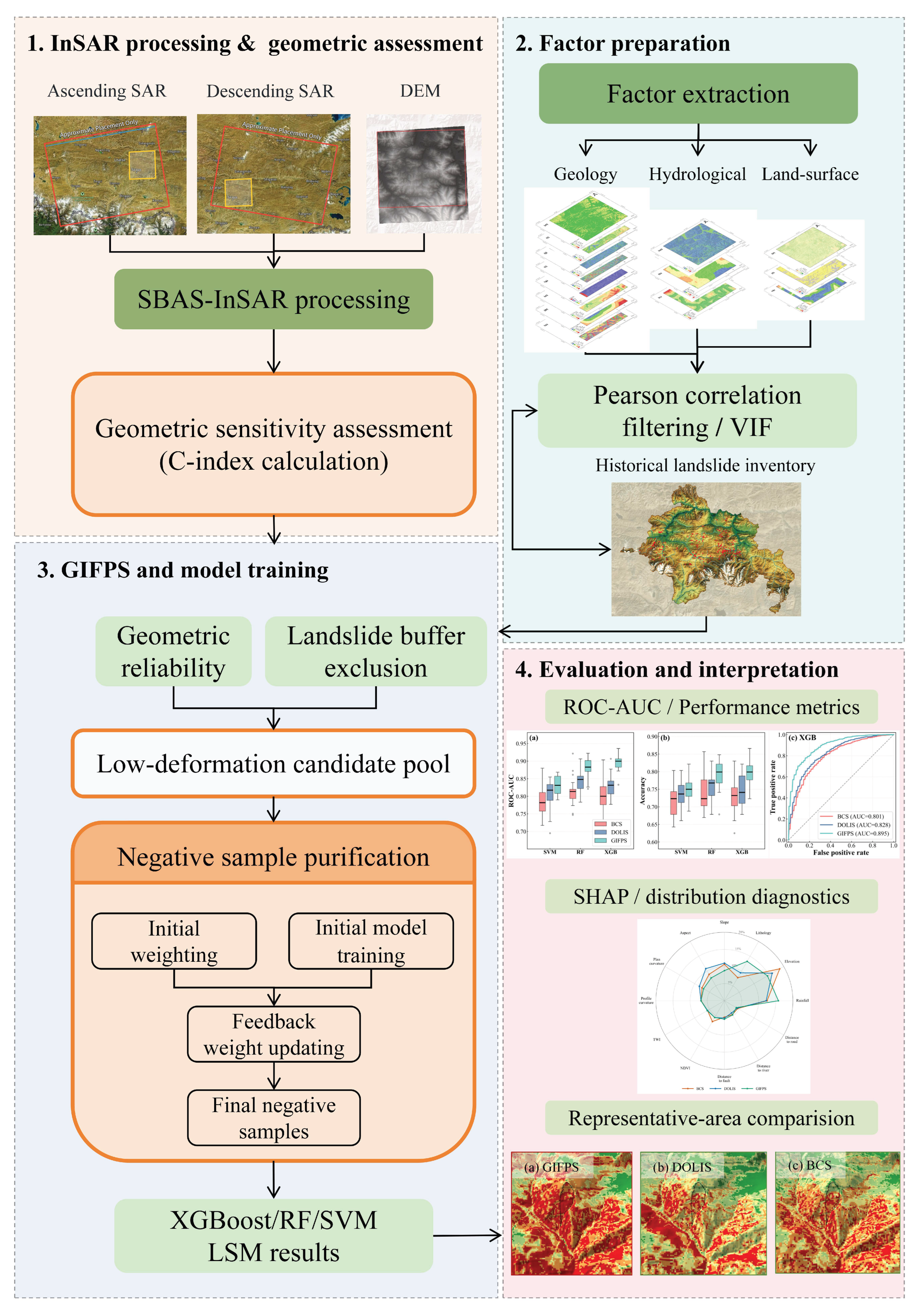
Figure 2 illustrates the overall workflow of this study. The workflow consists of four main components: SBAS-InSAR processing and geometric sensitivity assessment, landslide conditioning factor preparation, GIFPS-based negative sample selection, and model evaluation and interpretation. First, ascending and descending SBAS-InSAR deformation results are generated, and the C-index is calculated from satellite viewing geometry and DEM-derived topographic information. Second, landslide conditioning factors are extracted and screened using Pearson correlation analysis and variance inflation factor (VIF), while the historical landslide inventory is used to define positive samples. Third, GIFPS is applied to construct reliable negative samples by combining integrated low-deformation information, C-index-based geometric sensitivity, and model-feedback weighting. Finally, the resulting susceptibility models are evaluated using repeated sampling experiments, performance metrics, SHAP analysis, sample-distribution diagnostics, and representative-area comparison.

3.1. SBAS-InSAR Surface Deformation Monitoring

The SBAS-InSAR technique adopts a multi-master strategy and the small-baseline principle to construct an interferometric network with short temporal and spatial baselines [43]. Through this strategy, SBAS-InSAR can mitigate spatial decorrelation effects and obtain long-term time series of ground deformation. It has been widely used to monitor subtle ground deformation over large areas [44,45], such as landslide monitoring. The standard SBAS-InSAR workflow in SARscape 5.7.0 includes the application of precise orbit data, co-registration, subsetting, interferogram generation, removal of flat-earth and topographic phases, phase filtering, phase unwrapping, refinement and re-flattening, time-series inversion, and geocoding. After the unwrapped interferograms are refined and re-flattened to reduce residual orbital ramps and phase trends, SBAS inversion is performed to estimate LOS deformation rates and displacement time series.
For the study area, separate LOS velocity fields are obtained from the ascending and descending orbit datasets and subsequently used for negative sample selection.

3.2. Conditioning Factor Screening

Section 2.3 presents 14 initially selected conditioning factors associated with landslide occurrence, covering topographic, geological, hydrometeorological, and human-activity-related conditions. Pearson correlation analysis and the VIF are used together to reduce redundant factors and improve the quality of the model inputs.
Pearson correlation analysis is first used to examine the linear relationship between pairs of conditioning factors [46]:
r x y = i = 1 n x i x y i y i = 1 n x i x 2 i = 1 n y i y 2
where x i and y i refer to the values of the two factors, with x and y denoting their mean values and n the sample size. Pearson’s correlation coefficient r 1,1 , and r increases with the strength of correlation [47].
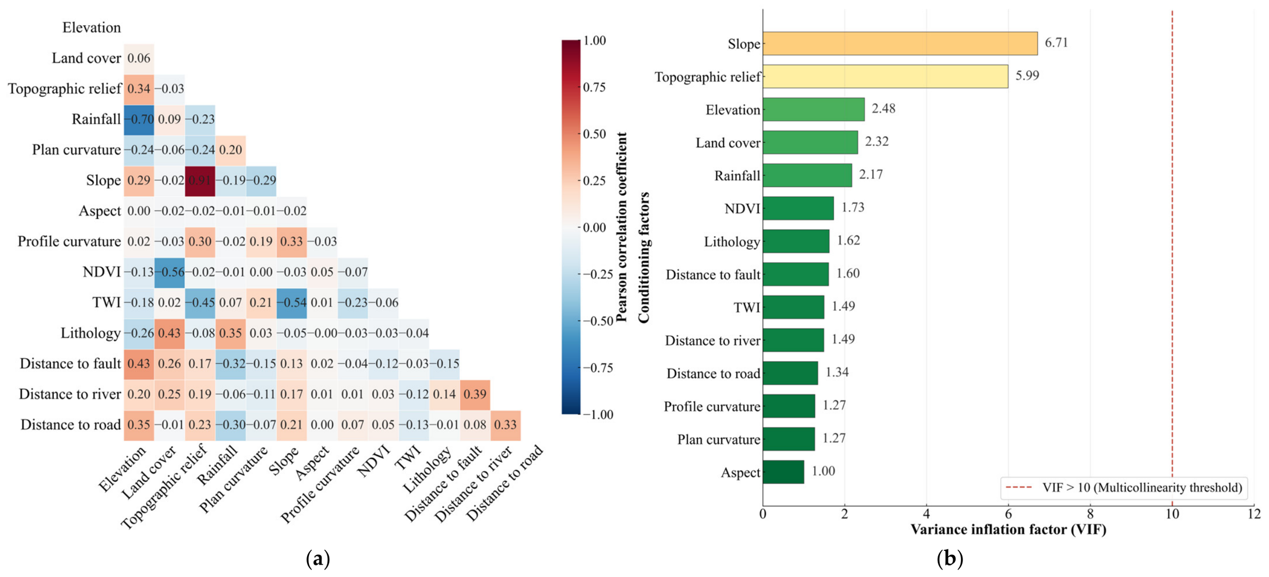
Generally, an absolute Pearson correlation coefficient greater than 0.7 between two factors is considered to indicate a strong linear relationship. In this study, topographic relief and slope show a significant correlation (correlation coefficient = 0.91; Figure 3a).
The VIF is then used to further quantify multicollinearity among the factors, and it is defined as:
V I F j = 1 1 R j 2
where R j 2 is the coefficient of determination when performing an auxiliary regression with x j as the dependent variable and the other factors as independent variables. A VIF value greater than 10 usually indicates severe multicollinearity among factors [48]. The VIF values of the factors selected in this study are all less than 10. Among them, slope and topographic relief exhibit relatively high VIF values (Figure 3b). Considering both the Pearson correlation coefficient and VIF results, since topographic relief refers to the elevation difference per unit area, while slope refers to the steepness of a slope with a more direct physical meaning, topographic relief is removed. The remaining static factors are included in model training.

3.3. Geometry-Aware InSAR Feedback Purification Sampling

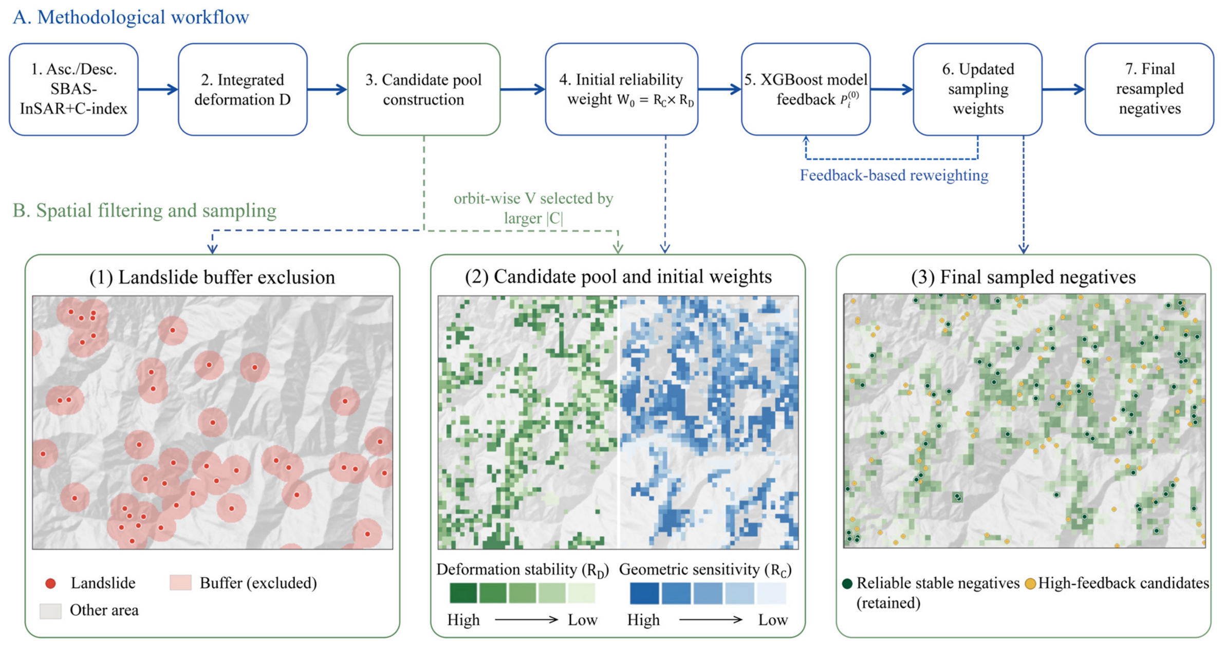
The GIFPS strategy consists of seven sequential stages (Figure 4). First, ascending and descending SBAS-InSAR results and the corresponding C-index layers are used to generate an integrated deformation layer. Based on this layer, a candidate negative sample pool is defined after excluding the buffers around historical landslides. Second, each candidate pixel is assigned an initial reliability weight by combining deformation stability and C-index-based geometric sensitivity. Third, an XGBoost model is trained to provide feedback on the similarity between candidate pixels and known landslides, and the sampling weights are updated accordingly. The final negative samples are then resampled from the weighted candidate pool. Through this workflow, GIFPS aims to improve negative sample reliability while preserving the representativeness of the candidate pool in terms of landslide conditioning factors.

3.3.1. Construction of the Candidate Negative Sample Pool

The candidate negative sample pool is constructed from ascending and descending SBAS-InSAR deformation results. Because LOS deformation is affected by radar viewing geometry, the C-index is calculated separately for the two tracks. For each track, the sign of the C-index indicates the expected LOS projection direction under the assumed steepest downslope movement, whereas its absolute value represents the magnitude of LOS geometric sensitivity [49]. Under this assumption, a |C| value closer to 1 indicates that a given magnitude of downslope movement produces a larger LOS projection and is therefore more readily expressed in the observed LOS deformation rate. Conversely, when |C| is close to 0, even substantial downslope movement may produce only a weak LOS signal. For each pixel, the LOS deformation rate from the track with the larger absolute C-index is selected as the composite LOS deformation rate to retain the observation with more favorable sensitivity to the assumed downslope movement. Thus, the C-index quantitatively characterizes the LOS geometric sensitivity of ascending and descending InSAR observations, enabling GIFPS to prioritize deformation measurements acquired under more favorable observation geometry during calculation.
Because candidate-pool construction is based on deformation intensity rather than inferred movement direction or sign consistency between the ascending and descending observations, the deformation intensity is defined as D i = | V i |, where V i denotes the selected composite LOS deformation rate. The D i values are classified into five classes using the natural breaks method, and the upper boundary of the lowest-deformation class is defined as D low . A pixel is included in the candidate negative sample pool if D i D low and it is located outside the 1000 m buffer around historical landslide points. The same buffer distance is applied consistently to all negative sample selection strategies included in the comparative experiments to ensure comparability.
The resulting pool is not interpreted as a set of verified non-landslide samples or stable locations. Rather, it represents relatively reliable inactive or low-deformation candidate samples during the InSAR monitoring period. Low observed LOS deformation indicates only that no obvious deformation is detected in the observable LOS component during that period; it does not exclude future slope movement. The candidate labels are therefore provisional and are further refined through C-index-based geometric-sensitivity weighting and model-feedback reweighting in the subsequent steps.

3.3.2. Determination of Initial Sampling Weights

For each candidate pixel, an initial sampling reliability weight is calculated by combining deformation stability and LOS geometric sensitivity. Deformation stability is defined as:
R D , i = 1 D i D low
where D i is the composite deformation intensity of candidate pixel i and D low is the upper boundary of the lowest deformation class. A smaller deformation magnitude corresponds to higher stability reliability. R D , i is constrained to the range [0, 1].
The geometric sensitivity of the pixel is represented by the C-index:
R C , i = C i
In the local east–north–up (E, N, U) coordinate system, the C-index of pixel i can be calculated from the SAR incidence angle, satellite heading angle, and DEM-derived slope geometry. Following Dai et al. [50], it is defined as:
C i = c o s γ = m p
where m is the unit vector in the LOS direction and p is the slope-direction vector along the steepest descent direction:
m = m E m N m U = s i n θ c o s β s i n θ s i n β c o s θ
p = p E p N p U = s i n α c o s δ c o s α c o s δ s i n δ
where θ is the incidence angle, β is the satellite flight azimuth (heading) angle, α is the slope aspect, and δ is the slope angle. Candidate negative samples with both low deformation intensity and high geometric sensitivity are therefore assigned higher sampling probabilities.
The initial sampling weight W i ( 0 ) is defined as:
W i ( 0 ) = R C , i R D , i
which represents the preliminary reliability of each candidate pixel and is used for weighted resampling before model-feedback adjustment.

3.3.3. Model Feedback Purification

Low deformation and favorable observation geometry do not necessarily indicate low landslide susceptibility. Some candidate pixels may have terrain, geological, or land-cover conditions similar to known landslides, making them unsuitable as high-confidence negative samples. To address this issue, model feedback is further introduced to revise the candidate weights.
First, negative samples equal in number to the training landslide samples are drawn from the candidate pool according to the initial weights W i ( 0 ) . These negative samples and the training landslide samples are then used to train an initial susceptibility model. The sampling weights are used only to control the probability of selecting negative samples. Once selected, positive and negative samples are assigned equal weights during model training.
For each candidate pixel, the trained model produces a predicted susceptibility probability P i ( 0 ) . A high P i ( 0 ) indicates that the landslide conditioning factors of the candidate pixel are similar to those of positive samples, and its reliability as a negative sample should therefore be assigned a lower relative sampling preference. The feedback-corrected sampling weight is calculated as:
W i ( 1 ) = W i ( 0 ) + 1 P i ( 0 ) 2
where W i ( 1 ) is the revised sampling weight after model feedback. The final negative samples are then drawn according to W i ( 1 ) and are combined with the training landslide samples to train the final susceptibility model.
Only one round of model-feedback correction is used in this study. This design introduces information from the conditioning factors as a correction to the InSAR-geometry-based initial weights, while avoiding excessive dependence on model-derived probabilities through repeated iterations. Repeatedly updating unlabeled samples using model predictions may lead to error accumulation in semi-supervised learning [51], which is not the aim of this strategy.

3.4. XGBoost Model

At the beginning of each repetition, the 184 historical landslide samples are randomly divided into training and testing subsets at a 7:3 ratio. The candidate pool for each strategy is constructed using the training landslide locations and then divided into disjointed training and testing subsets. Negative samples are drawn separately to match the corresponding numbers of positive samples, while model feedback and final model fitting use only the training data.
XGBoost is used as the main classifier in this study. It is a gradient-boosting framework based on decision-tree ensembles and has been widely used in LSA [52]. XGBoost builds weak decision trees sequentially and improves model fitting by learning the gradients of the loss function from previous iterations. It also includes a regularization term to reduce overfitting. Because of its ability to handle nonlinear relationships, variable interactions, and limited sample sizes, XGBoost is suitable for relatively small and heterogeneous training datasets.
For a binary classification problem, the objective function of XGBoost at the t -th iteration can be written as:
L t = i = 1 n l y i , y ^ i t 1 + f t x i + Ω f t
where l is the loss function, f t x i is the output of the t -th tree, and Ω f t is the regularization term. By minimizing this objective function, the model progressively improves the separation between landslide and non-landslide conditions. Then, the additive tree output is transformed into the predicted susceptibility probability P i .

3.5. Spatial Block Cross-Validation

To examine whether the model comparison is affected by spatial autocorrelation, an additional five-fold spatial block cross-validation is conducted using XGBoost. The study area is divided into regular square blocks with side lengths of 5 and 10 km. At each spatial scale, the blocks are assigned to five outer folds while maintaining approximately balanced numbers of historical landslide points among the folds. In each validation round, four folds are used for training, and the remaining fold is retained for testing, with each fold serving as the test set once. To further reduce spatial proximity between the training and testing samples, the test blocks and a surrounding 1000 m guard zone are excluded from the training candidate negative sample pools.
Within each fold, the low-deformation thresholds used by GIFPS and DOLIS are derived from the training region and applied unchanged to the test blocks. Negative samples in the test blocks are selected according to the corresponding sampling strategy. The final performance at each spatial scale is obtained by averaging the fold-level metrics across the five folds.

3.6. Evaluation Metrics

Model performance is evaluated using ROC-AUC, accuracy, precision, recall, and F1-score. In addition, the standardized mean difference (SMD), Kolmogorov–Smirnov (KS) statistic, and normalized Wasserstein distance are used to examine the factor distributions of the selected negative samples.

3.6.1. ROC Curve and AUC

TP, FP, TN, and FN denote true positives, false positives, true negatives, and false negatives, respectively. The ROC curve is defined by the true positive rate (TPR) versus the false positive rate (FPR):
T P R = T P T P + F N
F P R = F P F P + T N
The area under the ROC curve (AUC) is
A U C = 0 1 T P R F P R d F P R

3.6.2. Confusion-Matrix-Based Metrics

Accuracy:
A c c u r a c y = TP + TN TP + FP + TN + FN
Precision:
Precision = TP TP + FP
Recall:
Recall = TP TP + FN
F1-score:
F 1 = 2 Precision Recall Precision + Recall

3.6.3. Sample-Distribution Diagnostics

For the j -th conditioning factor, the SMD is calculated as:
S M D j = μ s , j μ c , j σ s , j 2 + σ c , j 2 / 2
The KS statistic is calculated as:
K S j = s u p x F s , j x F c , j x
The normalized Wasserstein distance N W j is calculated as:
N W j = W j x j , m a x x j , m i n
where the subscripts s and c denote the selected negative samples and the candidate negative sample pool, respectively, μ and σ are the mean and standard deviation, F x is the empirical cumulative distribution function, W j is the first-order Wasserstein distance, and x j , m a x and x j , m i n are the maximum and minimum values of factor j . Smaller SMD, KS, and N W values indicate that the selected negative samples better preserve the conditioning factor distributions of the candidate pool.

4. Results

4.1. SBAS-InSAR and Geometric Sensitivity Results

In this study, ascending and descending Sentinel-1 data are processed using the SBAS-InSAR workflow implemented in ENVI SARscape 5.7.0. The interferometric network is constructed with maximum temporal and perpendicular baselines of 48 days and 200 m, respectively, and the 30 m Copernicus DEM is used for topographic phase removal. A product coherence threshold of 0.20 is applied during SBAS processing, and phase unwrapping is performed using the Delaunay Minimum Cost Flow (MCF) algorithm with an unwrapping coherence threshold of 0.25. During the second inversion, pixels are required to have at least 65% valid interferograms and 90% valid acquisitions. Atmospheric phase artifacts are reduced using spatiotemporal filtering with a spatial low-pass size of 1600 m and a temporal high-pass size of 365 days. During geocoding, a temporal coherence threshold of 0.15 and a velocity-precision threshold of 8 mm/yr are applied. These parameters influence the extraction of low-deformation pixels in two ways. The valid-observation, temporal-coherence, and velocity-precision thresholds primarily determine which pixels are retained for subsequent analysis, whereas phase unwrapping and atmospheric filtering may also affect the estimated deformation rates.
Spatiotemporal filtering is intended to reduce atmospheric components according to their spatial and temporal characteristics, but deformation signals with similar characteristics may also be attenuated. Residual phase-unwrapping errors may likewise introduce discontinuities or biases into the estimated deformation rates. The adopted filtering, unwrapping, and quality-control settings are intended to reduce these effects but cannot eliminate them completely. Pixels failing the quality-control criteria are treated as invalid and excluded before deformation classification rather than being assigned to the low-deformation class. After screening, usable deformation measurements cover 97.2% and 94.4% of the study area for the ascending and descending datasets, respectively.
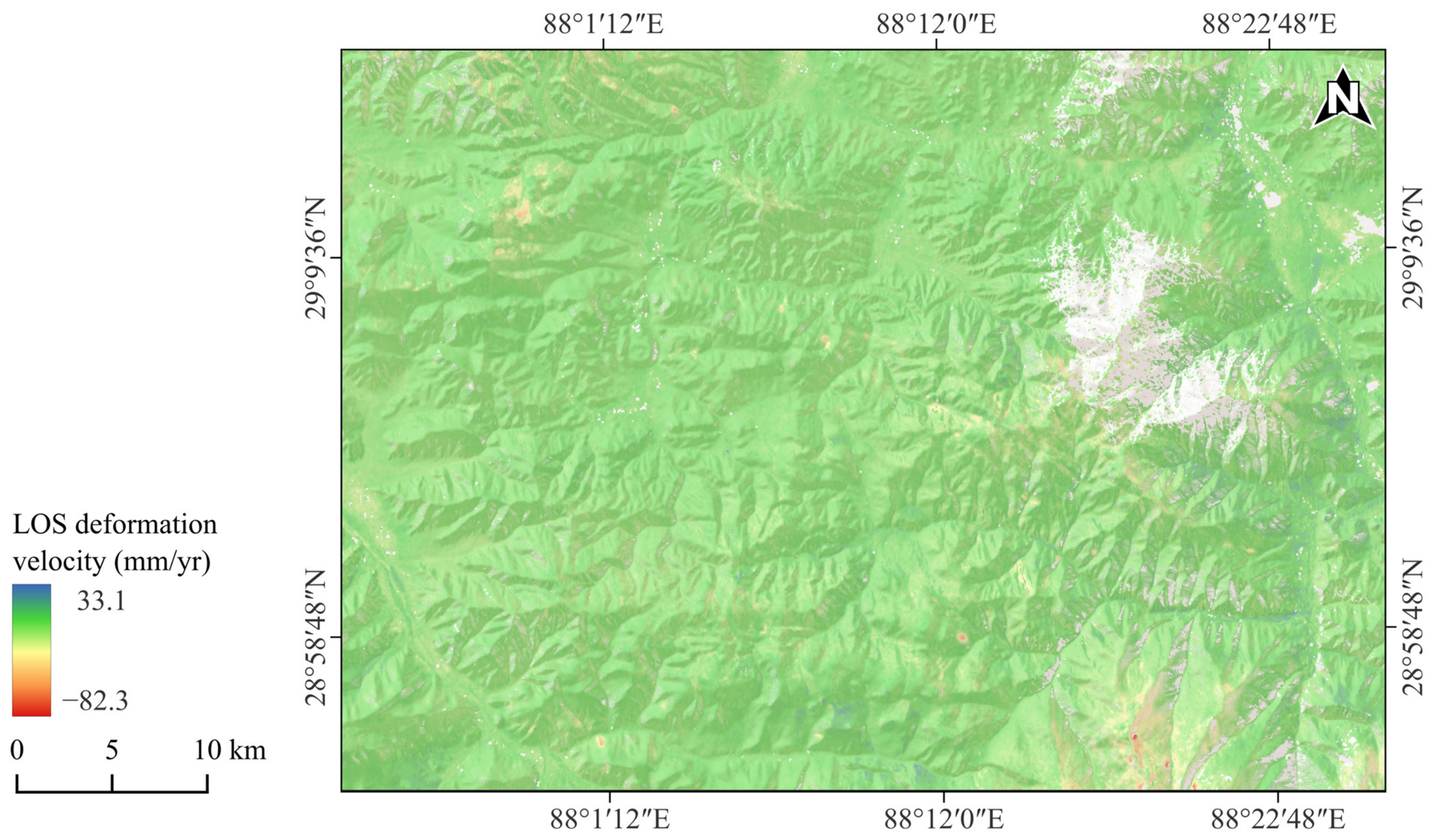
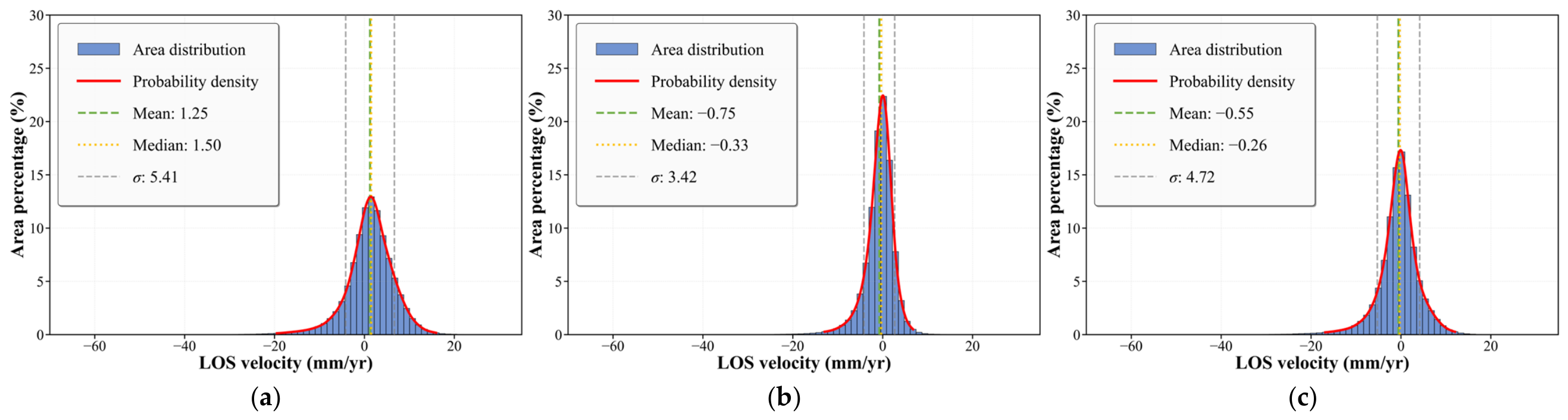
To examine possible topography-correlated atmospheric residuals, Pearson correlation coefficients are calculated between DEM elevation and the corrected cumulative displacement. The absolute correlation coefficients decrease from 0.119 to 0.051 for the ascending track and from 0.097 to 0.093 for the descending track. After correction, the R2 values are below 0.01 for both tracks, indicating that the remaining correlations with elevation are weak. Pixel-level uncertainty is further examined using the RMSE and Vprecision fields exported by SARscape. The median Vprecision is 2.28 mm/yr for the ascending dataset and 3.02 mm/yr for the descending dataset, whereas the corresponding median RMSE values are 1.50 and 1.97 mm. The mean annual LOS deformation rate ranges from −80.2 to 40.2 mm/yr for the ascending data and from −82.3 to 42.5 mm/yr for the descending data. In both tracks, the deformation-rate distributions are concentrated around 0, indicating that most pixels show limited observed LOS deformation during the monitoring period (Figure 5a,b).
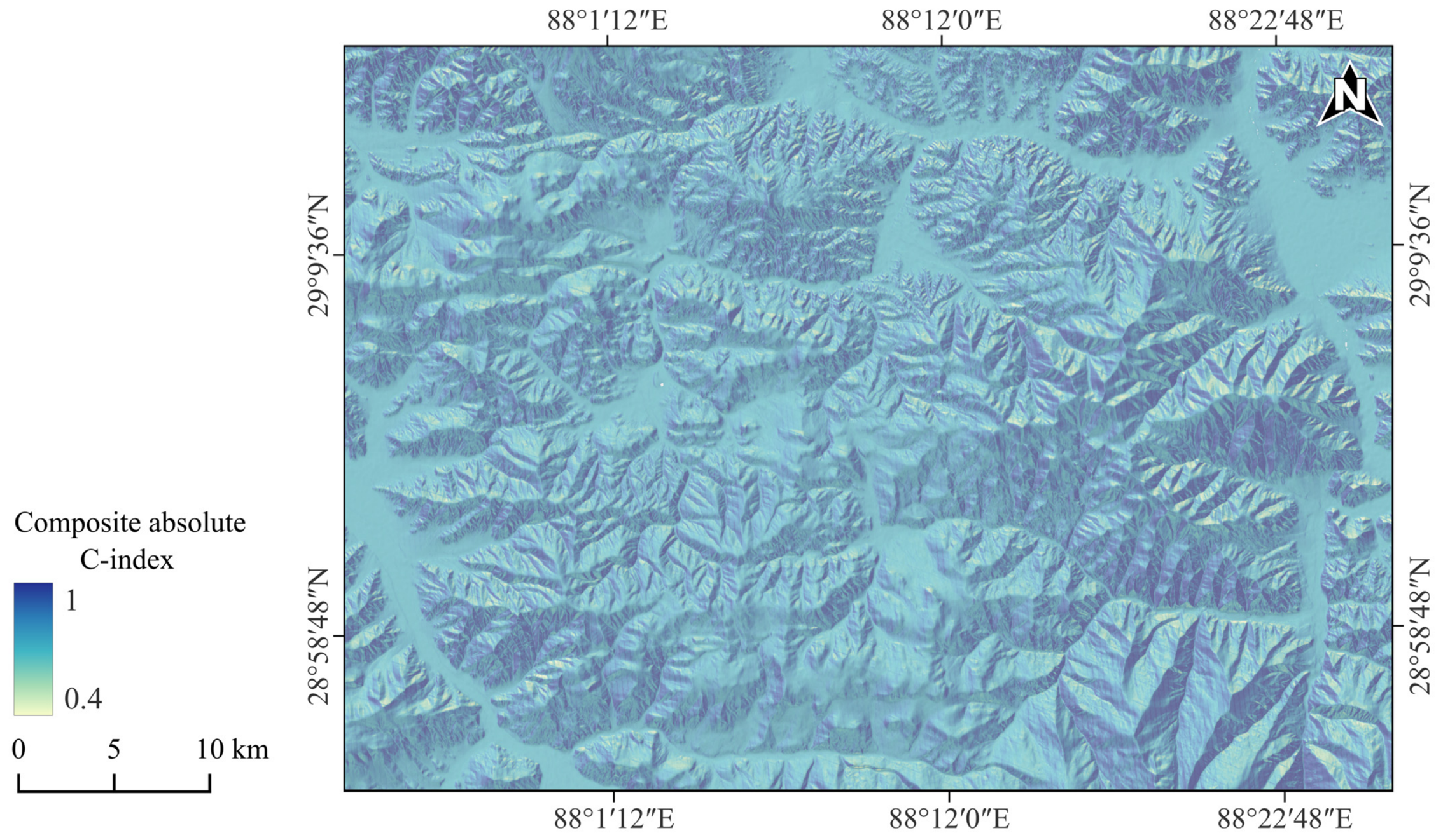
Single-track InSAR measurements are constrained by SAR viewing geometry. Therefore, the ascending and descending results are integrated using the C-index criterion described in Section 3.3.1. The resulting deformation-intensity distribution remains centered around 0, with most pixels falling within a narrow low-deformation range, although localized anomalies are still present (Figure 5c). The corresponding composite absolute C-index is shown in Figure 6. This layer represents the absolute C-index value of the selected orbit for each pixel, that is, the ascending or descending track used to construct the composite deformation result. It indicates the LOS geometric sensitivity associated with the integrated deformation layer.
As shown in Figure 7, low-deformation pixels are widely distributed across the study area, whereas higher deformation values are mainly concentrated in the Quga–Ganglongmang area or occur as scattered anomalies. The lowest-deformation class identified using the natural breaks method accounts for approximately 44.4% of the valid pixels and is used to define the preliminary candidate negative sample pool. Because low LOS deformation does not necessarily indicate slope stability, the sampling reliability of these candidates is subsequently refined using C-index-based geometric sensitivity and model feedback.

4.2. Performance of the Landslide Susceptibility Mapping

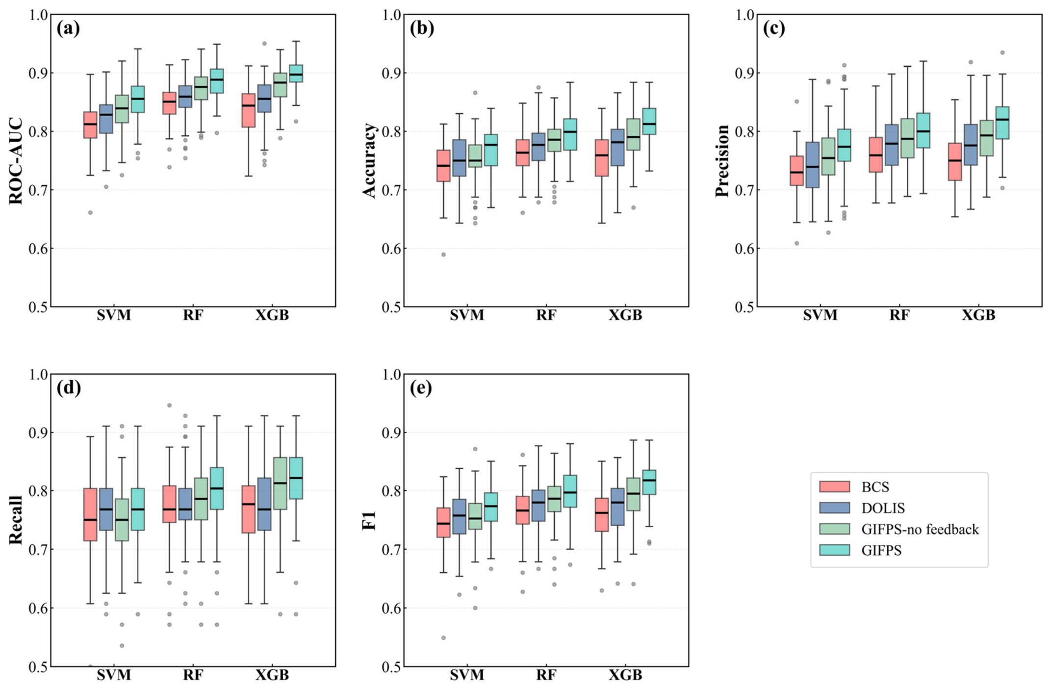
To assess how the selection of negative samples influences model performance, GIFPS is compared with BCS and dual-orbit low-deformation intersection sampling (DOLIS). BCS randomly selects negative samples outside the 1000 m buffers surrounding historical landslides [53], whereas DOLIS selects negative samples from the intersection of the lowest absolute-deformation classes of the ascending and descending tracks through natural-breaks classification [54,55]. An ablation variant without model feedback, termed GIFPS-no feedback, is also included to evaluate the contribution of the model-feedback mechanism. Three classifiers, including support vector machine (SVM), random forest (RF), and XGBoost, are used for comparison. For each classifier, negative samples are independently resampled 100 times to conduct repeated experiments. Model performance is evaluated using ROC-AUC, accuracy, precision, recall, and F1-score.
The predefined hyperparameter ranges are provided in Supplementary Table S1, and the final selected settings are summarized in Table 2. A randomized parameter search is conducted using five-fold stratified cross-validation, with ROC-AUC as the optimization criterion. The selected settings are then kept fixed across BCS, DOLIS, GIFPS-no feedback, and GIFPS throughout all 100 repeated experiments, allowing the comparison to focus on the effects of the negative sample selection strategies.
Figure 8 shows the performance distributions of the different model combinations across repeated independent experiments, while Table 3 reports the corresponding mean values. Overall, GIFPS achieves the best performance across all three classifiers, particularly in terms of ROC-AUC and F1-score. Compared with BCS, GIFPS increases the mean ROC-AUC and F1-score by 4.77 percentage points and 3.75 percentage points, respectively. Compared with DOLIS, the corresponding improvements are 3.58 percentage points and 2.59 percentage points, respectively.
The ablation results further distinguish the contribution of model feedback from that of C-index-based initial weighting. GIFPS-no feedback retains the low-deformation constraint and C-index-based initial weights but excludes feedback-based weight adjustment. Compared with this variant, the complete GIFPS increases the mean ROC-AUC and F1-score across the three classifiers by 1.77 and 1.70 percentage points, respectively. Paired Wilcoxon signed-rank tests confirm that the ROC-AUC and F1-score improvements are statistically significant for each classifier (all p < 0.001). These results indicate that the performance improvement of the model is driven jointly by the geometric constraints of the C-index and the model feedback.
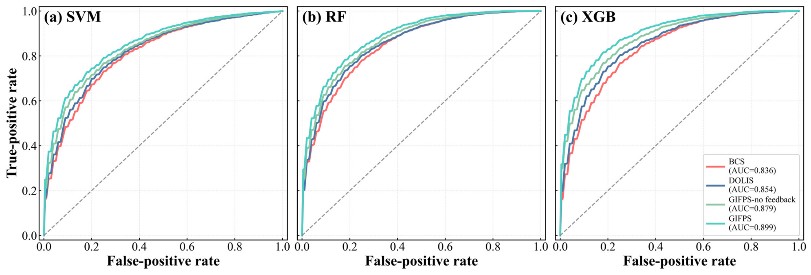
The ROC curves in Figure 9 further support these results. For all three classifiers, the curves obtained with the complete GIFPS are generally above those of BCS, DOLIS, and GIFPS-no feedback over most false-positive-rate ranges. The paired Wilcoxon signed-rank tests based on the 100 repetitions show that GIFPS achieves statistically significant ROC-AUC improvements under all three classifiers (p < 0.001). Among all classifier–sampling combinations, XGBoost combined with GIFPS produces the best overall performance and is therefore selected for subsequent landslide susceptibility mapping and spatial interpretation.
Additional sensitivity analyses are conducted to examine the effects of candidate-pool definition (Supplementary Tables S2 and S3). Across different buffer-distance settings, GIFPS consistently outperforms BCS and DOLIS in both ROC-AUC and F1-score, indicating that its relative advantage is not restricted to a single buffer distance. Based on the reported areas of the inventoried landslides, the maximum equivalent circular radius is approximately 750 m; therefore, a 1000 m buffer provides a more conservative spatial exclusion around the recorded landslide locations. At the 1000 m buffer distance, alternative low-deformation definitions based on the 20th percentile and a fixed threshold of 5 mm/yr show no statistically significant differences from the natural-breaks threshold in either ROC-AUC or F1-score (p > 0.05). These results indicate that the relative performance improvement of GIFPS remains robust across the tested candidate-pool settings.

4.3. Results of Landslide Susceptibility Mapping

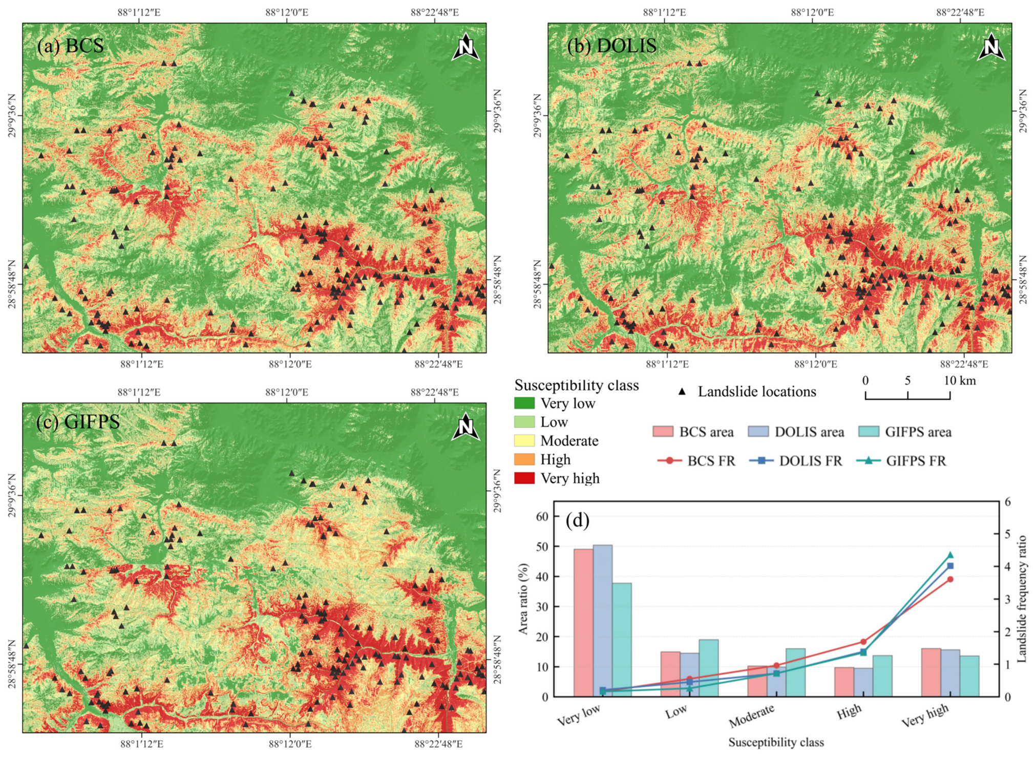
To further compare the spatial zonation obtained with different negative sampling strategies, susceptibility results generated by BCS, DOLIS, and GIFPS are divided into five classes according to the Jenks natural-breaks algorithm. For each class, both the area proportion and the frequency ratio (FR) are calculated. The FR is computed as the percentage of historical landslide points within a given susceptibility class divided by the areal proportion of that class. Values greater than 1 indicate an enrichment of historical landslides in that class. An increasing FR from low- to high-susceptibility classes therefore reflects consistency between the mapped susceptibility pattern and the locations of inventoried landslides.
Figure 10 illustrates that the high- and very-high-susceptibility zones derived from BCS, DOLIS, and GIFPS are mainly distributed around areas where historical landslide points are clustered. This pattern shows that all three negative sample selection strategies reproduce the broad spatial organization of landslide susceptibility across the study region.
The FR results show a general increase with susceptibility level for all three methods, suggesting that the zonation results are broadly reasonable. Within this common pattern, GIFPS performs better at both ends of the susceptibility scale. Within the very-low and low classes, GIFPS has lower FR than BCS and DOLIS, meaning that fewer historical landslides are included in areas classified as low susceptibility and that the low-susceptibility classes contain fewer inventoried landslides, indicating better separation among the susceptibility classes. Conversely, GIFPS yields the largest FR for the very-high class, although this class occupies a slightly smaller proportion of the study area than its BCS and DOLIS counterparts. Thus, the improved concentration of inventoried landslides is achieved without increasing the extent of the very-high-susceptibility class. Rather, it identifies a higher concentration of historical landslides within a smaller area.
Synthesizing its performance at both ends of the spectrum, GIFPS simultaneously minimizes the erroneous inclusion of historical landslides in low-susceptibility zones while maximizing the identification of historical landslides in very-high-susceptibility zones, thereby widening the disparity in FR between the low- and high-susceptibility categories. This indicates that, without compromising the integrity of the primary spatial patterns or expanding the spatial extent of high-susceptibility zones, GIFPS successfully achieves a superior discriminative capability in susceptibility zonation.

5. Discussion

5.1. Effect of GIFPS on Sample Selection and Model Behavior

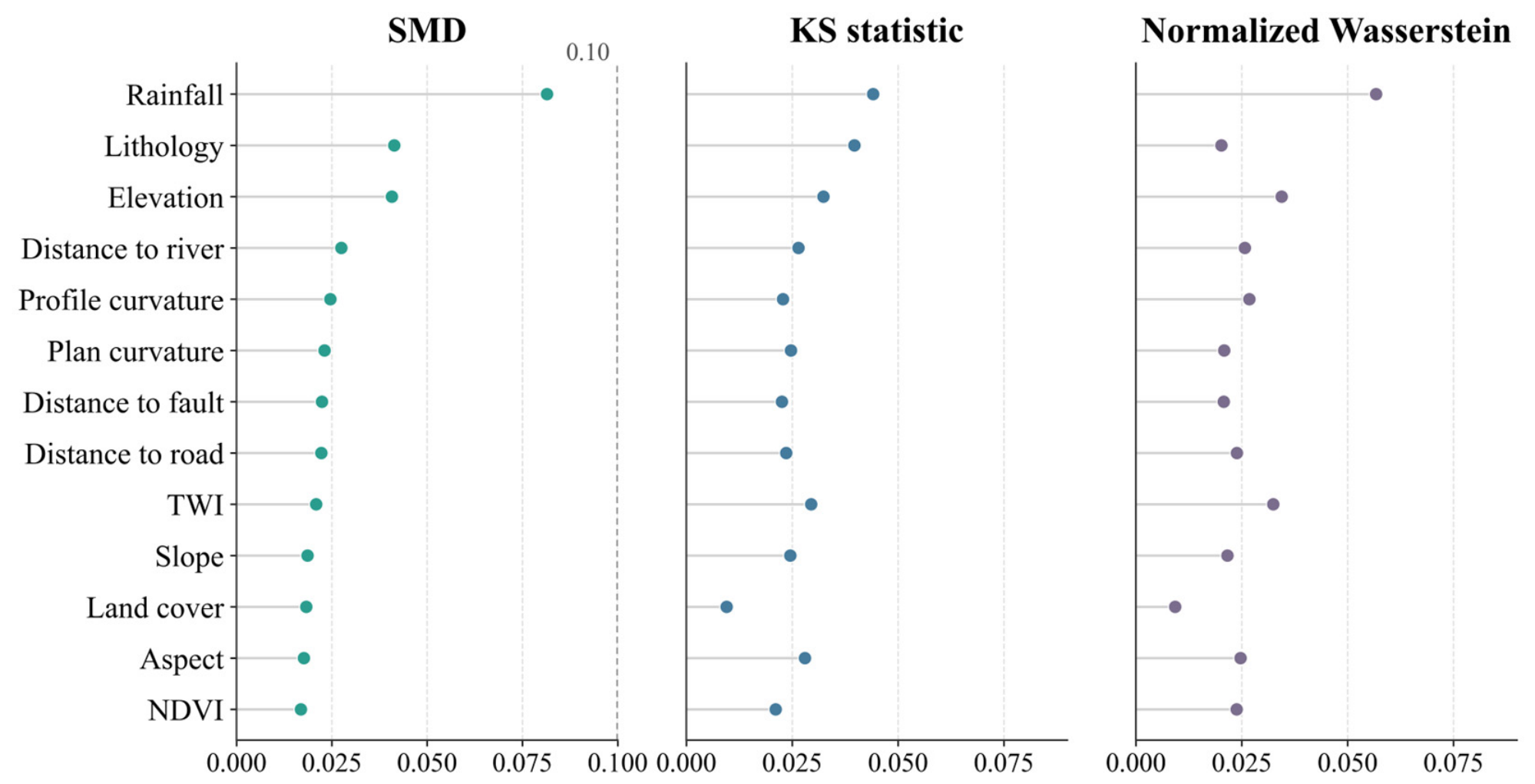
To investigate whether GIFPS induces a significant shift in the sample distribution, the final negative samples selected by GIFPS are compared with the GIFPS candidate pool using the SMD, the KS statistic, and the normalized Wasserstein distance (Figure 11). SMD is commonly used as a balance diagnostic, and an absolute SMD below 0.1 is often used as a reference threshold for negligible distributional imbalance [56]. Among all conditioning factors, rainfall shows the largest deviation. Nevertheless, the magnitude of this deviation remains limited. The SMD for rainfall is still below 0.1, and the corresponding KS statistic and normalized Wasserstein distance are also low. This indicates that GIFPS does not improve model performance by sharply narrowing the range of conditioning-factor values represented by the negative samples. Instead, it makes a moderate redistribution within the low-deformation candidate pool.
The improvement brought by GIFPS is therefore more likely related to improved negative sample reliability than to an artificial simplification of the classification task. The low-deformation constraint derived from InSAR provides information on slope deformation during the monitoring period. The C-index reduces the risk of treating areas with weak observed LOS deformation under poor observation geometry as stable zones. The model-feedback step further adjusts the sampling weights based on the similarity of the conditioning factors between candidate pixels and known landslides, assigning lower updated weights to highly similar candidates. Together, these steps produce a more reliable negative sample set while preserving the representativeness of its conditioning-factor distributions.
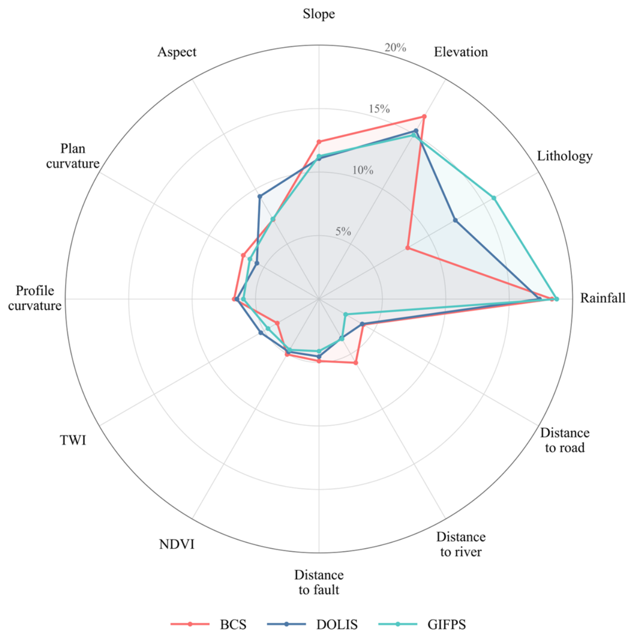
We further apply SHAP to examine feature contributions under different negative sample selection strategies. SHAP is an interpretability framework derived from Shapley values in game theory and assigns each feature an additive contribution to the model output. It has been widely used to interpret LSM results [57,58,59]. The relative SHAP importance values of the top 12 conditioning factors are presented in Figure 12. The dominant factors identified under the three sampling strategies are broadly consistent. Rainfall ranks first under BCS, DOLIS, and GIFPS, with relative contributions of 18.36%, 17.38%, and 18.74%, respectively. Elevation, lithology, slope, and aspect also rank among the leading factors across all three strategies.
Although the principal factors are similar, their relative contributions differ among the sampling strategies. GIFPS assigns a higher relative contribution to lithology (15.92%) than BCS (8.07%) and DOLIS (12.41%), whereas the contribution of elevation is slightly lower under GIFPS (14.91%) than under BCS (16.60%) and DOLIS (15.31%). These differences indicate that negative sample selection affects the relative attribution of model predictions among the conditioning factors.
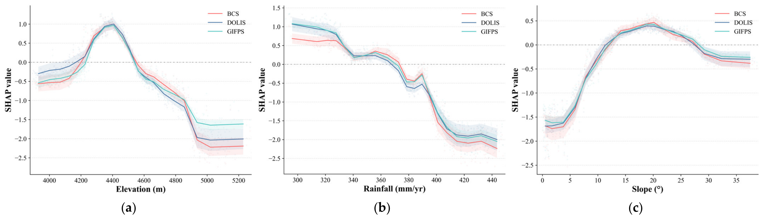
To further examine how the SHAP contributions vary across the observed ranges of individual conditioning factors, comparative dependence plots are generated for rainfall, elevation, and slope using the same reference sample set (Figure 13). The three sampling strategies produce broadly similar nonlinear curve shapes, while their differences are mainly reflected in the magnitude of the SHAP values. Thus, GIFPS changes the relative contribution assigned to several conditioning factors without substantially altering the overall dependence relationships learned by the model. As SHAP attribution can be affected by sample composition, correlations among factors, and model structure, these results are used to compare model behavior rather than to infer causal effects.

5.2. Spatial Interpretation in Representative Landslide Areas

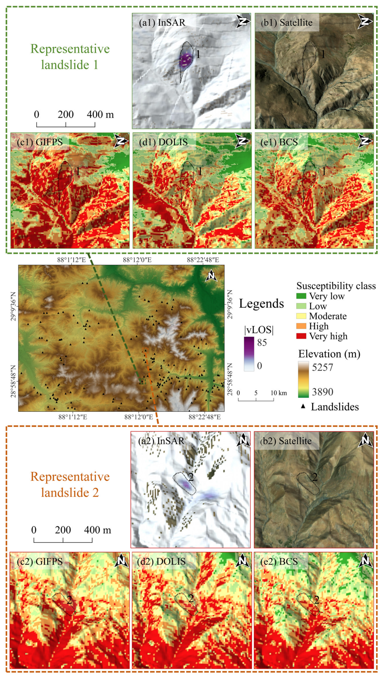
Two historical landslide areas are selected to compare the spatial susceptibility patterns produced by the different methods. The two cases differ in landslide scale and geomorphic setting (Table 4), but both are located in alpine canyon terrain with strong relief and evident slope deformation. Figure 14 compares the susceptibility maps generated by GIFPS, DOLIS, and BCS with the SBAS-InSAR deformation results and satellite imagery.
The SBAS-InSAR results show that both landslide areas exhibit locally concentrated deformation signals. These deforming zones are mainly located within the historical landslide bodies or in their immediate surroundings. Compared with BCS and DOLIS, GIFPS produces more pronounced high-susceptibility patterns around the landslide-affected slopes. In representative landslide area 1, the high-susceptibility zones mapped by GIFPS extend continuously along the main disturbed slope and correspond more closely to the InSAR deformation signals. In representative landslide area 2, GIFPS also delineates a clearer high-susceptibility pattern around the landslide body. By contrast, the results from BCS and DOLIS are more fragmented or show weaker contrast between the landslide-affected slopes and the surrounding background areas. These spatial patterns suggest that GIFPS improves not only numerical model performance but also the spatial contrast of the resulting susceptibility map.
This difference is closely related to how negative samples are selected. BCS selects negative samples mainly by excluding areas around inventoried landslides, but it does not consider whether the remaining background area is deforming, nor does it assess whether low deformation signals are reliable under the local SAR viewing geometry. DOLIS uses low-deformation InSAR information, but it still largely treats low LOS deformation as an indicator of slope stability. GIFPS adds two further constraints: LOS geometric sensitivity and model feedback. These constraints reduce the probability of selecting unreliable pixels, or pixels with conditioning factors similar to known landslides, as negative samples. As a result, the model trained with GIFPS produces susceptibility patterns that are more consistent with both the geomorphic expression of historical landslides and the observed deformation signals.

5.3. Effect of Spatial Autocorrelation on Model Evaluation

Spatial block cross-validation geographically separates the training and testing samples, thereby reducing the influence of their spatial proximity on model evaluation (Table 5). At the 5 km block size, GIFPS achieves a mean ROC-AUC of 0.8372, exceeding 0.7940 for BCS and 0.7807 for DOLIS. At the 10 km block size, the corresponding values are 0.8228, 0.7847, and 0.7789, respectively. Although these ROC-AUC values are lower than the 0.8986 achieved by XGBoost–GIFPS under random splitting, GIFPS retains the highest mean ROC-AUC at both block sizes.
Compared with random splitting, all methods show lower overall performance under spatial block cross-validation, indicating that greater geographic separation between the training and testing samples increases the difficulty of model prediction. At the 10 km block size, GIFPS does not outperform BCS across all metrics, as its recall and F1-score are lower. This may be associated with greater differences in the distributions of conditioning factors between the training and testing folds at the larger block size. Consequently, some landslide samples may receive predicted probabilities below the fixed classification threshold, although GIFPS retains the highest overall ranking ability, as indicated by ROC-AUC. Overall, these results suggest that the performance improvement of GIFPS is not entirely attributable to the spatial proximity permitted by random splitting. Nevertheless, its predictive performance in geographically separated areas, particularly under stronger spatial heterogeneity, requires further evaluation.

5.4. Comparison with Previous Studies and Limitations

Existing approaches reduce negative sample uncertainty through PU learning [60], geographic-environment similarity constraints [61], or InSAR-informed deformation constraints [62]. InSAR-assisted sampling introduces deformation information during the monitoring period, but weak LOS deformation may also result from unfavorable radar viewing geometry. Related studies have therefore used the C-index or other InSAR sensitivity indices to evaluate the detectability and geometric sensitivity of landslide deformation [63]. However, these indices have mainly been used for InSAR applicability assessment or landslide detection rather than for constructing and reweighting negative samples in LSA. GIFPS extends this idea by using the C-index to select the more geometrically sensitive LOS observation, using the resulting low-deformation pixels to define the candidate pool, and incorporating LOS geometric sensitivity and model feedback into the sampling weights. It therefore combines monitoring-period deformation, observation geometry, and conditioning-factor feedback within a unified negative sample selection strategy.
However, several limitations should be acknowledged. First, the low-deformation candidate areas identified by GIFPS represent slopes showing no pronounced LOS movement during the monitoring period, rather than independently verified stable areas. Dormant but susceptible slopes may therefore remain in the candidate pool and affect the resulting classification. Second, the C-index is calculated under the assumption that potential movement is approximately aligned with the steepest downslope direction. This assumption is more applicable to shallow translational landslides but may be less reliable for rotational, compound, or structurally controlled landslides [64]. The C-index should therefore be interpreted as an indicator of potential LOS geometric sensitivity rather than a reconstruction of the actual movement direction. In addition, GIFPS remains dependent on the completeness and positional accuracy of the historical landslide inventory. Although InSAR information reduces the likelihood of selecting uninventoried deforming slopes as negative samples, inventory errors may still affect model training.
Uncertainty in the SBAS-InSAR deformation results may also propagate into the sampling process. Residual atmospheric delays, phase-unwrapping errors, temporal decorrelation, and geometric distortions can affect deformation estimates, particularly in high-altitude mountainous areas [65]. Furthermore, spatial block cross-validation shows that GIFPS retains the highest ROC-AUC at both spatial scales examined, although its recall and F1-score do not exceed those of BCS at the 10 km scale. Its transferability to regions where the conditioning-factor distributions differ from those of the training area therefore requires further evaluation.
The practical implementation of GIFPS requires ascending and descending SAR time series, a historical landslide inventory, DEM-derived slope geometry, conditioning-factor datasets, and sufficient computational resources for SBAS-InSAR processing and repeated model training. Although the main satellite and terrain datasets used in this study are publicly available, dual-orbit InSAR processing requires greater computational resources and technical expertise than conventional buffer-controlled sampling [66]. Where only one SAR track is available, deformation intensity and C-index-based geometric sensitivity can still be used, but orbit selection is no longer possible and additional criteria may be required to account for the limited geometric sensitivity. Where InSAR observations are unavailable, conditioning-factor similarity analysis or physics-informed slope-stability constraints may provide an alternative basis for negative sample selection [67,68]. High-resolution optical satellite imagery and field-based monitoring may also help to alleviate data limitations in these regions [69].
From a practical perspective, GIFPS is intended to support regional susceptibility screening rather than deterministic slope-stability assessment or real-time early warning. The resulting maps can help geological hazard agencies and transportation authorities to prioritize monitoring activities and infrastructure assessments. Future work should apply the method to areas with different geomorphic and climatic settings and combine it with field investigations, unmanned aerial vehicle (UAV) photogrammetry, and global navigation satellite system (GNSS) monitoring to further evaluate its applicability and physical reliability. As SAR technology advances, high-resolution spaceborne spotlight or sliding spotlight observations may provide more detailed deformation information in localized landslide-prone areas [70]. These observations could serve as optional data sources for refining candidate negative sample selection.

6. Conclusions

This study proposes a GIFPS strategy to address negative sample uncertainty in data-driven landslide susceptibility assessment. The method integrates ascending and descending SBAS-InSAR deformation information, C-index-based geometric sensitivity, and model feedback into the negative sample selection process to reduce the probability of selecting potentially unstable slopes as negative samples. Experiments are conducted in the Shigatse region, leading to the following conclusions:
(1)
In terms of predictive performance, GIFPS outperforms the commonly used BCS method and DOLIS. Across SVM, RF, and XGBoost classifiers, GIFPS achieves higher ROC-AUC and F1-score values. The improvement is confirmed by repeated experiments and Wilcoxon signed-rank tests. Ablation experiments further indicate that removing model feedback leads to a consistent decrease in performance, confirming its contribution within the GIFPS framework.
(2)
The susceptibility map generated using GIFPS shows better spatial discrimination. The very-high-susceptibility zones contain a higher proportion of historical landslide points within a relatively limited area, while the low-susceptibility zones contain fewer historical landslide points. This indicates that GIFPS improves the spatial separation between susceptibility classes.
(3)
From the perspectives of sample-distribution diagnostics and model interpretation, GIFPS alters the relative contributions of the conditioning factors but does not substantially narrow their distributions in the final negative samples relative to the candidate pool. The SMD, KS statistic, and normalized Wasserstein distance consistently indicate that the final negative samples largely preserve the conditioning-factor distributions of the candidate pool. Therefore, the performance gain of GIFPS is more likely attributable to improved negative sample reliability than to an artificially simplified classification task.
Overall, GIFPS provides an interpretable InSAR-assisted approach for negative sample selection in LSA in complex alpine canyon areas. Future work should test its applicability in different regional settings and combine it with field investigation or GNSS monitoring to further evaluate its physical reliability and generalizability.

Supplementary Materials

The following supporting information can be downloaded at: https://www.mdpi.com/article/10.3390/rs18152591/s1, Table S1: Hyperparameter search ranges; Table S2: Performance comparison of BCS, DOLIS, and GIFPS under different buffer distances. Values are means (standard deviations) across 30 independent repetitions; Table S3: Sensitivity of GIFPS to alternative low-deformation threshold definitions at the 1000 m buffer distance. Values are means (standard deviations) across 30 independent repetitions.

Author Contributions

Conceptualization, H.C. and C.Z.; methodology, H.C., J.D. and Y.S.; software, H.C.; validation, H.C., C.Z. and J.D.; formal analysis, H.C., Y.C. and Y.S.; investigation, J.D. and Y.L.; resources, Y.L. and Y.C.; data curation, H.C. and Y.C.; writing—original draft preparation, H.C.; writing—review and editing, C.Z., J.D. and Y.L.; visualization, H.C.; supervision, C.Z. and J.D.; project administration, Y.L.; funding acquisition, Y.L. All authors have read and agreed to the published version of the manuscript.

Funding

This research was funded by the Open Project Program of Innovation Base for Monitoring, Evaluation, and Early Warning Technology of Territorial Space Ecological Restoration in the Southern Hilly and Mountainous Region of China, Chinese Geological Society (Grant No. CSZX-JD202503); Fundamental Research Funds for the Central Universities, China University of Geosciences (Wuhan) (No. 202510491064).

Data Availability Statement

The reproducibility materials supporting this study are available through Zenodo at https://doi.org/10.5281/zenodo.21483682. The repository contains the sampling and analysis code, random-seed rules, model parameters, experimental settings, study-area boundary, derived InSAR and C-index rasters, a representative candidate-pool raster, numerical results. The remaining datasets used in this study are publicly available from the sources specified in the manuscript.

Conflicts of Interest

The authors declare no conflicts of interest.

References

  1. Niyokwiringirwa, P.; Gall, T.; Jha, A.K. Toward a Standard for Landslide Data: Bridging Gaps in Landslide Susceptibility Modeling and Early Warning Systems; World Bank: Washington, DC, USA, 2026; Available online: https://documents.worldbank.org/en/publication/documents-reports/documentdetail/099321402252610889 (accessed on 20 July 2026).
  2. Duan, Y.; Ding, M.; He, Y.; Zheng, H.; Delgado-Téllez, R.; Sokratov, S.; Dourado, F.; Fuchs, S. Global Projections of Future Landslide Susceptibility under Climate Change. Geosci. Front. 2025, 16, 102074. [Google Scholar] [CrossRef] [Scilit]
  3. Zhang, Q.; Ma, W.; Gao, Y.; Zhang, T.; Ma, X.; Li, L.; Zhou, Q.; Liu, F. Zoning of the Disaster-Inducing Environment and Driving Factors for Landslides, Collapses, and Debris Flows on the Qinghai–Tibet Plateau. Appl. Sci. 2025, 15, 6569. [Google Scholar] [CrossRef] [Scilit]
  4. Zhao, B.; Su, L.; Xu, Q.; Li, W.; Xu, C.; Wang, Y. A Review of Recent Earthquake-Induced Landslides on the Tibetan Plateau. Earth-Sci. Rev. 2023, 244, 104534. [Google Scholar] [CrossRef] [Scilit]
  5. Dong, A.; Dou, J.; Fu, Y.; Zhang, R.; Xing, K. Unraveling the Evolution of Landslide Susceptibility: A Systematic Review of 30-Years of Strategic Themes and Trends. Geocarto Int. 2023, 38, 2256308. [Google Scholar] [CrossRef] [Scilit]
  6. Tran, V.A.; Khuc, T.D.; Truong, X.Q.; Nguyen, A.B.; Phi, T.T. Application of Potential Machine Learning Models in Landslide Susceptibility Assessment: A Case Study of Van Yen District, Yen Bai Province, Vietnam. Quat. Sci. Adv. 2024, 14, 100181. [Google Scholar] [CrossRef] [Scilit]
  7. Rai, S.C.; Pandey, V.K.; Sharma, K.K.; Sharma, S. Landslide Susceptibility Analysis in the Bhilangana Basin (India) Using GIS-Based Machine Learning Methods. Geosyst. Geoenviron. 2024, 3, 100253. [Google Scholar] [CrossRef] [Scilit]
  8. Yao, J.; Yao, X.; Zhao, Z.; Liu, X. Performance Comparison of Landslide Susceptibility Mapping under Multiple Machine-Learning Based Models Considering InSAR Deformation: A Case Study of the Upper Jinsha River. Geomat. Nat. Hazards Risk 2023, 14, 2212833. [Google Scholar] [CrossRef] [Scilit]
  9. Guo, Z.; Tian, B.; Zhu, Y.; He, J.; Zhang, T. How Do the Landslide and Non-Landslide Sampling Strategies Impact Landslide Susceptibility Assessment?—A Catchment-Scale Case Study from China. J. Rock Mech. Geotech. Eng. 2024, 16, 877–894. [Google Scholar] [CrossRef] [Scilit]
  10. Liu, Q.; Tang, A.; Huang, D. Exploring the Uncertainty of Landslide Susceptibility Assessment Caused by the Number of Non–Landslides. CATENA 2023, 227, 107109. [Google Scholar] [CrossRef] [Scilit]
  11. Huang, F.; Mao, D.; Jiang, S.-H.; Zhou, C.; Fan, X.; Zeng, Z.; Catani, F.; Yu, C.; Chang, Z.; Huang, J.; et al. Uncertainties in Landslide Susceptibility Prediction Modeling: A Review on the Incompleteness of Landslide Inventory and Its Influence Rules. Geosci. Front. 2024, 15, 101886. [Google Scholar] [CrossRef] [Scilit]
  12. Huang, F.; Xiong, H.; Jiang, S.-H.; Yao, C.; Fan, X.; Catani, F.; Chang, Z.; Zhou, X.; Huang, J.; Liu, K. Modelling Landslide Susceptibility Prediction: A Review and Construction of Semi-Supervised Imbalanced Theory. Earth-Sci. Rev. 2024, 250, 104700. [Google Scholar] [CrossRef] [Scilit]
  13. Hong, H.; Wang, D.; Zhu, A.-X.; Wang, Y. Landslide Susceptibility Mapping Based on the Reliability of Landslide and Non-Landslide Sample. Expert Syst. Appl. 2024, 243, 122933. [Google Scholar] [CrossRef] [Scilit]
  14. Yang, Y.; Zhang, R.; Wang, T.; Liu, A.; He, Y.; Lv, J.; He, X.; Mao, W.; Xiang, W.; Zhang, B. An Information Quantity and Machine Learning Integrated Model for Landslide Susceptibility Mapping in Jiuzhaigou, China. Nat. Hazards 2024, 120, 10185–10217. [Google Scholar] [CrossRef] [Scilit]
  15. Yang, L.; Cui, Y.; Xu, C.; Ma, S. Application of Coupling Physics–Based Model TRIGRS with Random Forest in Rainfall-Induced Landslide-Susceptibility Assessment. Landslides 2024, 21, 2179–2193. [Google Scholar] [CrossRef] [Scilit]
  16. Gu, T.; Duan, P.; Wang, M.; Li, J.; Zhang, Y. Effects of Non-Landslide Sampling Strategies on Machine Learning Models in Landslide Susceptibility Mapping. Sci. Rep. 2024, 14, 7201. [Google Scholar] [CrossRef] [Scilit] [PubMed]
  17. Wei, R.; Li, Y.; Li, Y.; Wang, Z.; Wu, C.; Wang, J.; Zhang, B.; Ye, C. Edge-Attentive Graph Convolutional Network and Positive-Unlabeled Framework for Landslide Susceptibility Mapping. Gondwana Res. 2025, 148, 240–254. [Google Scholar] [CrossRef] [Scilit]
  18. Cui, Y.; Deng, Q.; Miao, H. Application of a Relief-Optimized Method for Target Space Exteriorization Sampling in Landslide Susceptibility Assessment. J. Mt. Sci. 2025, 22, 3391–3407. [Google Scholar] [CrossRef] [Scilit]
  19. Gu, X.; Li, Y.; Zuo, X.; Bu, J.; Yang, F.; Yang, X.; Li, Y.; Zhang, J.; Huang, C.; Shi, C.; et al. Image Compression–Based DS-InSAR Method for Landslide Identification and Monitoring of Alpine Canyon Region: A Case Study of Ahai Reservoir Area in Jinsha River Basin. Landslides 2024, 21, 2501–2517. [Google Scholar] [CrossRef] [Scilit]
  20. Li, Z.; Chen, B.; Liu, Y.; Peng, J.; Xu, Q.; Jiang, L.; Du, J.; Song, C.; Ding, M.; Zhu, W. Long-Term Three-Dimensional Deformation Monitoring and Risk Assessment of the Guba Landslide, Tibetan Plateau. Sci. China Earth Sci. 2025, 68, 3288–3305. [Google Scholar] [CrossRef] [Scilit]
  21. Ran, S.; Zhou, W.; Weng, Y.; Chi, F.; Wang, D.; Cao, X.; Ma, G. Causative Environment-Informed Active Landslide Detection with InSAR Monitoring: Empowering Reservoir Slope Hazard Management. Int. J. Appl. Earth Obs. Geoinf. 2026, 146, 105079. [Google Scholar] [CrossRef] [Scilit]
  22. Cheng, Y.; Pang, H.; Li, Y.; Fan, L.; Wei, S.; Yuan, Z.; Fang, Y. Applications and Advancements of Spaceborne InSAR in Landslide Monitoring and Susceptibility Mapping: A Systematic Review. Remote Sens. 2025, 17, 999. [Google Scholar] [CrossRef] [Scilit]
  23. Zhang, R.; Zhang, L.; Fang, Z.; Oguchi, T.; Merghadi, A.; Fu, Z.; Dong, A.; Dou, J. Interferometric Synthetic Aperture Radar (InSAR)-Based Absence Sampling for Machine-Learning-Based Landslide Susceptibility Mapping: The Three Gorges Reservoir Area, China. Remote Sens. 2024, 16, 2394. [Google Scholar] [CrossRef] [Scilit]
  24. Liu, Z.; Zhang, Z.; Zhang, W.; Ren, J.; Chen, Q. InSAR-Based Landslide Susceptibility Analysis in Karst Erosion Landforms Using a Non-Landslide Sampling Strategy. Int. J. Appl. Earth Obs. Geoinf. 2025, 145, 104997. [Google Scholar] [CrossRef] [Scilit]
  25. Xu, S.; Song, Y.; Lu, P.; Mu, G.; Yang, K.; Wang, S. An Optimized Non-Landslide Sampling Method for Landslide Susceptibility Evaluation Using Machine Learning Models. Nat. Hazards 2025, 121, 5873–5900. [Google Scholar] [CrossRef] [Scilit]
  26. Hanssen, R.F. Stochastic Model for Radar Interferometry. In Radar Interferometry: Data Interpretation and Error Analysis; Springer: Dordrecht, The Netherlands, 2001; pp. 81–159. [Google Scholar]
  27. Sharifi, S.; Macciotta, R.; Hendry, M.; Rotheram-Clarke, D.; Huntley, D. Evaluating Topography-Based Methods in 3D Decomposition of InSAR 1D Velocities Obtained for Translational Landslides: Thompson River Valley in Canada. Landslides 2024, 21, 411–427. [Google Scholar] [CrossRef] [Scilit]
  28. Guo, R.; Li, S.; Chen, Y.; Li, X.; Yuan, L. Identification and Monitoring Landslides in Longitudinal Range-Gorge Region with InSAR Fusion Integrated Visibility Analysis. Landslides 2021, 18, 551–568. [Google Scholar] [CrossRef] [Scilit]
  29. Yang, S.; Li, D.; Liu, Y.; Xu, Z.; Sun, Y.; She, X. Landslide Identification in Human-Modified Alpine and Canyon Area of the Niulan River Basin Based on SBAS-InSAR and Optical Images. Remote Sens. 2023, 15, 1998. [Google Scholar] [CrossRef] [Scilit]
  30. Torre, D.; Galve, J.P.; Reyes-Carmona, C.; Alfonso-Jorde, D.; Ballesteros, D.; Menichetti, M.; Piacentini, D.; Troiani, F.; Azañón, J.M. Geomorphological Assessment as Basic Complement of InSAR Analysis for Landslide Processes Understanding. Landslides 2024, 21, 1273–1292. [Google Scholar] [CrossRef] [Scilit]
  31. Plank, S.; Singer, J.; Minet, C.; Thuro, K. Pre-Survey Suitability Evaluation of the Differential Synthetic Aperture Radar Interferometry Method for Landslide Monitoring. Int. J. Remote Sens. 2012, 33, 6623–6637. [Google Scholar] [CrossRef] [Scilit]
  32. Zhang, J.; Zuo, X.; Li, Y.; Shi, M.; Shi, C.; Huang, C.; Tang, X. Detection and Assessment of Potential Landslides in the Xiaojiang River Basin Using SBAS-InSAR. Sci. Rep. 2025, 15, 16082. [Google Scholar] [CrossRef] [Scilit] [PubMed]
  33. Li, X.; Fan, Q.; Niu, Y.; Zhang, S.; Zhao, J.; Si, J.; Wang, Z.; Ju, Z.; Lu, Z. A Two-Dimensional InSAR-Based Framework for Landslide Identification and Movement Pattern Classification. Remote Sens. 2025, 17, 3889. [Google Scholar] [CrossRef] [Scilit]
  34. Sun, K.; Li, Z.; Wang, S.; Hu, R. A Support Vector Machine Model of Landslide Susceptibility Mapping Based on Hyperparameter Optimization Using the Bayesian Algorithm: A Case Study of the Highways in the Southern Qinghai–Tibet Plateau. Nat. Hazards 2024, 120, 11377–11398. [Google Scholar] [CrossRef] [Scilit]
  35. Huang, F.; Liu, K.; Jiang, S.; Catani, F.; Liu, W.; Fan, X.; Huang, J. Optimization Method of Conditioning Factors Selection and Combination for Landslide Susceptibility Prediction. J. Rock Mech. Geotech. Eng. 2025, 17, 722–746. [Google Scholar] [CrossRef] [Scilit]
  36. Sajadi, P.; Sang, Y.-F.; Gholamnia, M.; Bonafoni, S.; Mukherjee, S. Evaluation of the Landslide Susceptibility and Its Spatial Difference in the Whole Qinghai-Tibetan Plateau Region by Five Learning Algorithms. Geosci. Lett. 2022, 9, 9. [Google Scholar] [CrossRef] [Scilit]
  37. Zhang, C. 1:100000 Geological Hazard Distribution Data of China Nepal Transportation Corridor (2022–2023). 2023. Available online: https://data.tpdc.ac.cn/zh-hans/data/f252a14d-91d9-4fed-9b7b-638c671d6399 (accessed on 16 January 2026).
  38. Xu, X. China Active Fault Database. 2023. Available online: https://github.com/gmt-china/china-geospatial-data/releases (accessed on 16 January 2026).
  39. Steinshouer, D.W.; Qiang, J.; McCabe, P.J.; Ryder, R.T. Maps Showing Geology, Oil and Gas Fields, and Geologic Provinces of the Asia Pacific Region. 1999. Available online: https://pubs.usgs.gov/of/1997/ofr-97-470/OF97-470F/ (accessed on 17 January 2026).
  40. Zanaga, D.; Van De Kerchove, R.; De Keersmaecker, W.; Souverijns, N.; Brockmann, C.; Quast, R.; Wevers, J.; Grosu, A.; Paccini, A.; Vergnaud, S.; et al. ESA WorldCover 10 m 2020 V100. 2021. Available online: https://zenodo.org/record/5571936 (accessed on 9 February 2026).
  41. Yue, D. Grid Dataset of Meteorological Elements for 1km of China Nepal Transportation Corridor (1992–2022). 2024. Available online: https://data.tpdc.ac.cn/zh-hans/data/e5daef81-b973-4cce-b7e8-82a0ad03dfc8 (accessed on 18 January 2026).
  42. Zhao, B. China-Nepal Transport Corridor 1:10 00000 Stream Data Set (2017). 2017. Available online: https://data.tpdc.ac.cn/zh-hans/data/244f6fa0-ded1-4a29-9c21-3486405a2c8b (accessed on 16 January 2026).
  43. Berardino, P.; Fornaro, G.; Lanari, R.; Sansosti, E. A New Algorithm for Surface Deformation Monitoring Based on Small Baseline Differential SAR Interferograms. IEEE Trans. Geosci. Remote Sens. 2002, 40, 2375–2383. [Google Scholar] [CrossRef] [Scilit]
  44. Wang, F.; Wen, Z.; Gao, Q.; Yu, Q.; Li, D.; Chen, L. Thermokarst Landslides Susceptibility Evaluation across the Permafrost Region of the Central Qinghai-Tibet Plateau: Integrating a Machine Learning Model with InSAR Technology. J. Hydrol. 2024, 642, 131800. [Google Scholar] [CrossRef] [Scilit]
  45. Hussain, S.; Pan, B.; Hussain, W.; Sajjad, M.M.; Ali, M.; Afzal, Z.; Abdullah-Al-Wadud, M.; Tariq, A. Integrated PSInSAR and SBAS-InSAR Analysis for Landslide Detection and Monitoring. Phys. Chem. Earth Parts ABC 2025, 139, 103956. [Google Scholar] [CrossRef] [Scilit]
  46. Ullah, M.; Tang, B.; Huangfu, W.; Yang, D.; Wei, Y.; Qiu, H. Machine Learning-Driven Landslide Susceptibility Mapping in the Himalayan China–Pakistan Economic Corridor Region. Land 2024, 13, 1011. [Google Scholar] [CrossRef] [Scilit]
  47. Zhao, F.; Miao, F.; Wu, Y.; Ke, C.; Gong, S.; Ding, Y. Refined Landslide Susceptibility Mapping in Township Area Using Ensemble Machine Learning Method under Dataset Replenishment Strategy. Gondwana Res. 2024, 131, 20–37. [Google Scholar] [CrossRef] [Scilit]
  48. O’brien, R.M. A Caution Regarding Rules of Thumb for Variance Inflation Factors. Qual. Quant. 2007, 41, 673–690. [Google Scholar] [CrossRef] [Scilit]
  49. Xiong, Z.; Zhang, M.; Ma, J.; Xing, G.; Feng, G.; An, Q. InSAR-Based Landslide Detection Method with the Assistance of C-Index. Landslides 2023, 20, 2709–2723. [Google Scholar] [CrossRef] [Scilit]
  50. Dai, K.; Chen, Y.; Xu, Q.; Hancock, C.; Jiang, M.; Deng, J.; Zhuo, G. A Functional Model for Determining Maximum Detectable Deformation Gradients of InSAR Considering the Topography in Mountainous Areas. IEEE Trans. Geosci. Remote Sens. 2023, 61, 1–11. [Google Scholar] [CrossRef] [Scilit]
  51. Chen, B.; Jiang, J.; Wang, X.; Wan, P.; Wang, J.; Long, M. Debiased Self-Training for Semi-Supervised Learning. In Proceedings of the Advances in Neural Information Processing Systems; Koyejo, S., Mohamed, S., Agarwal, A., Belgrave, D., Cho, K., Oh, A., Eds.; Curran Associates, Inc.: Red Hook, NY, USA, 2022; Volume 35, pp. 32424–32437. [Google Scholar]
  52. Sahin, E.K. Assessing the Predictive Capability of Ensemble Tree Methods for Landslide Susceptibility Mapping Using XGBoost, Gradient Boosting Machine, and Random Forest. SN Appl. Sci. 2020, 2, 1308. [Google Scholar] [CrossRef] [Scilit]
  53. Tu, L.; Chen, M.; Leng, P.; Liu, S.; Liu, M.; Luo, W.; Mao, Y. Improving Landslide Susceptibility Assessment Through Non-Landslide Sampling Strategies. Land 2025, 14, 2059. [Google Scholar] [CrossRef] [Scilit]
  54. Shan, Y.; Xu, Z.; Zhou, S.; Lu, H.; Yu, W.; Li, Z.; Cao, X.; Li, P.; Li, W. Landslide Hazard Assessment Combined with InSAR Deformation: A Case Study in the Zagunao River Basin, Sichuan Province, Southwestern China. Remote Sens. 2023, 16, 99. [Google Scholar] [CrossRef] [Scilit]
  55. Qin, J.; Li, W.; Zhou, S.; Shan, Y.; He, G.; Fan, L. Optimizing Negative Sample Selection and Results for Landslide Susceptibility Assessment Using InSAR Surface Deformation. Geomat. Inf. Sci. Wuhan Univ. 2026, 51, 1228–1241. (In Chinese) [Google Scholar] [CrossRef]
  56. Austin, P.C. An Introduction to Propensity Score Methods for Reducing the Effects of Confounding in Observational Studies. Multivar. Behav. Res. 2011, 46, 399–424. [Google Scholar] [CrossRef] [Scilit] [PubMed]
  57. Wu, B.; Shi, Z.; Zheng, H.; Peng, M.; Meng, S. Impact of Sampling for Landslide Susceptibility Assessment Using Interpretable Machine Learning Models. Bull. Eng. Geol. Environ. 2024, 83, 461. [Google Scholar] [CrossRef] [Scilit]
  58. Zhao, F.; Miao, F.; Wu, Y.; Gong, S.; Qian, Z.; Zheng, G. Integration of Interpretable Machine Learning and MT-InSAR for Dynamic Enhancement of Landslide Susceptibility in the Three Gorges Reservoir Area. J. Rock Mech. Geotech. Eng. 2026, 18, 1193–1212. [Google Scholar] [CrossRef] [Scilit]
  59. Zhang, J.; Ma, X.; Zhang, J.; Sun, D.; Zhou, X.; Mi, C.; Wen, H. Insights into Geospatial Heterogeneity of Landslide Susceptibility Based on the SHAP-XGBoost Model. J. Environ. Manag. 2023, 332, 117357. [Google Scholar] [CrossRef] [Scilit] [PubMed]
  60. Fu, Z.; Ma, H.; Wang, F.; Dou, J.; Zhang, B.; Fang, Z. An Integrated Framework of Positive-Unlabeled and Imbalanced Learning for Landslide Susceptibility Mapping. IEEE J. Sel. Top. Appl. Earth Obs. Remote Sens. 2024, 17, 15596–15611. [Google Scholar] [CrossRef] [Scilit]
  61. Zhang, Q.; He, Y.; Zhang, L.; Lu, J.; Gao, B.; Yang, W.; Chen, H.; Zhang, Y. A Landslide Susceptibility Assessment Method Considering the Similarity of Geographic Environments Based on Graph Neural Network. Gondwana Res. 2024, 132, 323–342. [Google Scholar] [CrossRef] [Scilit]
  62. Liu, X.; Wang, S.; Liao, M. Landslide Susceptibility Assessment Incorporating Sample Optimization: A Case Study of Liujiaxia Reservoir Area. Remote Sens. Appl. Soc. Environ. 2026, 43, 102173. [Google Scholar] [CrossRef] [Scilit]
  63. Van Natijne, A.L.; Bogaard, T.A.; Van Leijen, F.J.; Hanssen, R.F.; Lindenbergh, R.C. World-Wide InSAR Sensitivity Index for Landslide Deformation Tracking. Int. J. Appl. Earth Obs. Geoinf. 2022, 111, 102829. [Google Scholar] [CrossRef] [Scilit]
  64. Bonì, R.; Bordoni, M.; Vivaldi, V.; Troisi, C.; Tararbra, M.; Lanteri, L.; Zucca, F.; Meisina, C. Assessment of the Sentinel-1 Based Ground Motion Data Feasibility for Large Scale Landslide Monitoring. Landslides 2020, 17, 2287–2299. [Google Scholar] [CrossRef] [Scilit]
  65. Wang, Y.; Dong, J.; Zhang, L.; Zhang, L.; Deng, S.; Zhang, G.; Liao, M.; Gong, J. Refined InSAR Tropospheric Delay Correction for Wide-Area Landslide Identification and Monitoring. Remote Sens. Environ. 2022, 275, 113013. [Google Scholar] [CrossRef] [Scilit]
  66. Li, S.; Xu, W.; Li, Z. Review of the SBAS InSAR Time-Series Algorithms, Applications, and Challenges. Geod. Geodyn. 2022, 13, 114–126. [Google Scholar] [CrossRef] [Scilit]
  67. Lu, J.; He, Y.; Zhang, L.; Zhang, Q.; Gao, B.; Chen, H.; Fang, Y. Ensemble Learning Landslide Susceptibility Assessment with Optimized Non-Landslide Samples Selection. Geomat. Nat. Hazards Risk 2024, 15, 2378176. [Google Scholar] [CrossRef] [Scilit]
  68. Liu, S.; Wang, L.; Zhang, W.; Sun, W.; Wang, Y.; Liu, J. Physics-Informed Optimization for a Data-Driven Approach in Landslide Susceptibility Evaluation. J. Rock Mech. Geotech. Eng. 2024, 16, 3192–3205. [Google Scholar] [CrossRef] [Scilit]
  69. Novellino, A.; Pennington, C.; Leeming, K.; Taylor, S.; Alvarez, I.G.; McAllister, E.; Arnhardt, C.; Winson, A. Mapping Landslides from Space: A Review. Landslides 2024, 21, 1041–1052. [Google Scholar] [CrossRef] [Scilit]
  70. Wu, B.; Liu, C.; Chen, J. A Review of Spaceborne High-Resolution Spotlight/Sliding Spotlight Mode SAR Imaging. Remote Sens. 2024, 17, 38. [Google Scholar] [CrossRef] [Scilit]
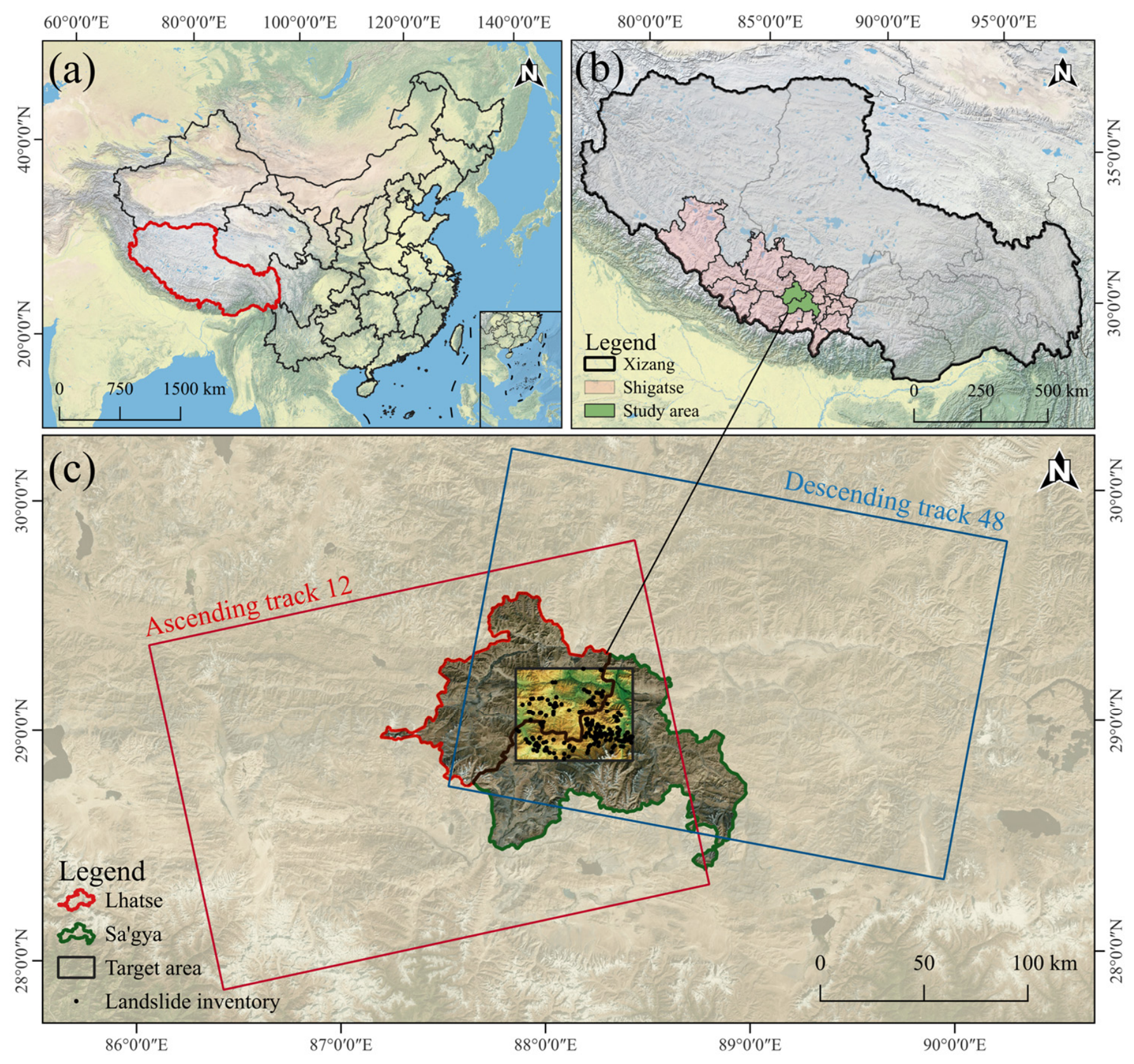
Figure 1. Location of the study area. (a) The location of the Xizang Autonomous Region in China. (b) The location of Shigatse City and the spatial distribution of Sa’gya County and Lhatse County within it. (c) The specific topography, historical landslide inventory, and the overlapping coverage footprints of the ascending and descending Sentinel-1 SAR orbits for the target area.
Remotesensing 18 02591 g001
Figure 2. Overall workflow.
Remotesensing 18 02591 g002
Figure 3. Correlation and multicollinearity analysis of landslide conditioning factors: (a) Pearson correlation heatmap; (b) VIF analysis, with bar colors changing from green to yellow as VIF values increase.
Remotesensing 18 02591 g003
Figure 4. Workflow of GIFPS for negative sample selection.
Remotesensing 18 02591 g004
Figure 5. Area-percentage histograms of SBAS-InSAR LOS deformation rates: (a) ascending-track deformation rate; (b) descending-track deformation rate; (c) integrated deformation rate.
Remotesensing 18 02591 g005
Figure 6. Spatial distribution of the composite absolute C-index associated with the integrated deformation layer.
Remotesensing 18 02591 g006
Figure 7. Spatial distribution of the integrated SBAS-InSAR LOS deformation rate based on C-index selection.
Remotesensing 18 02591 g007
Figure 8. Box plots of model performance across 100 independent repetitions: (a) ROC-AUC; (b) accuracy; (c) precision; (d) recall; (e) F1-score. Gray circles indicate outliers beyond the whiskers.
Remotesensing 18 02591 g008
Figure 9. Mean ROC curves obtained using BCS, DOLIS, GIFPS-no feedback, and GIFPS under three classifiers: (a) SVM; (b) RF; (c) XGBoost.
Remotesensing 18 02591 g009
Figure 10. Spatial distribution of landslide susceptibility and frequency-ratio comparison under different negative sample selection strategies: (a) BCS; (b) DOLIS; (c) GIFPS; (d) area ratio and frequency ratio of different susceptibility classes.
Remotesensing 18 02591 g010
Figure 11. Distributional deviation between GIFPS-selected negative samples and the GIFPS candidate pool measured by SMD, KS statistic, and normalized Wasserstein distance.
Remotesensing 18 02591 g011
Figure 12. Relative SHAP importance of the top 12 conditioning factors under BCS, DOLIS, and GIFPS.
Remotesensing 18 02591 g012
Figure 13. Comparative SHAP dependence plots for (a) elevation, (b) rainfall, and (c) slope under BCS, DOLIS, and GIFPS. Solid lines represent the binned mean responses, and shaded areas indicate the corresponding 95% confidence intervals.
Remotesensing 18 02591 g013
Figure 14. Representative-area comparison of SBAS-InSAR deformation, satellite imagery, and LSMs derived from different negative sample selection strategies. For representative landslides 1 and 2, panels (a1,a2) and (b1,b2) show the SBAS-InSAR deformation results and satellite images, respectively, while panels (c1,c2), (d1,d2), and (e1,e2) show the LSMs generated using GIFPS, DOLIS, and BCS, respectively. Numbers 1 and 2 denote the landslide IDs listed in Table 4.
Remotesensing 18 02591 g014
Table 1. Key parameters of Sentinel-1 data.
ParametersAscending DatasetDescending Dataset
SensorSentinel-1ASentinel-1A
Acquisition modeIWIW
Orbit directionAscendingDescending
Relative orbit (track)1248
Revisit period12 days12 days
PolarizationVVVV
Incidence angle43.78°43.11°
Pixel spacing
(range × azimuth)
2.33 m × 13.94 m2.33 m × 13.94 m
Radar wavelength5.6 cm5.6 cm
Table 2. Hyperparameter settings of the classifiers used in the model comparison.
ClassifierHyperparameterSetting
SVMKernelRBF
C10
Gamma0.03
Probability outputTrue
RFNumber of trees300
Maximum featuressqrt
Maximum depthNone
Minimum samples per leaf1
XGBoostNumber of trees100
Learning rate0.1
Maximum depth4
Subsample1
Column subsample1
Minimum child weight1
L2 regularization1
Objective functionbinary: logistic
Evaluation metriclogloss
Table 3. Quantitative performance comparison of different classifiers and negative sample selection strategies. Bold values indicate the best performance for each evaluation metric within each classifier.
ClassifierMethodROC-AUCAccuracyPrecisionRecallF1
RFBCS0.84900.76290.76150.76980.7639
DOLIS0.85770.77490.77780.77430.7745
GIFPS-no feedback0.87160.78300.78630.78180.7823
GIFPS0.88740.79700.80080.79500.7962
SVMBCS0.81080.73950.73120.75980.7437
DOLIS0.82040.74960.74540.76430.7528
GIFPS-no feedback0.83510.75260.75610.75200.7520
GIFPS0.85250.76970.77630.76290.7680
XGBoostBCS0.83570.75540.74910.77040.7581
DOLIS0.85300.77320.77590.77410.7731
GIFPS-no feedback0.87880.79190.78920.80000.7930
GIFPS0.89860.81410.81520.81640.8140
Table 4. Geomorphological parameters of typical historical landslide areas. The scale is defined by the historical landslide inventory.
IDScaleArea (m2)Relief (m)Max Elevation (m)Mean Elevation (m)Mean Slope (°)
1Large204,084.526749704845.421.3
2Medium93,411.616946554571.518.8
Table 5. Performance of different negative sample selection strategies under spatial block cross-validation. Bold values indicate the best result for each evaluation metric within each block size.
Block SizeMethodROC-AUCAccuracyPrecisionRecallF1-Score
5 kmBCS0.7940.72430.74290.71250.7184
DOLIS0.78070.70880.72950.6850.695
GIFPS0.83720.74330.75380.75070.7345
10 kmBCS0.78470.70450.71760.70140.7015
DOLIS0.77890.69020.71310.67720.6808
GIFPS0.82280.70620.74730.6790.6934
Disclaimer/Publisher’s Note: The statements, opinions and data contained in all publications are solely those of the individual author(s) and contributor(s) and not of MDPI and/or the editor(s). MDPI and/or the editor(s) disclaim responsibility for any injury to people or property resulting from any ideas, methods, instructions or products referred to in the content.