From Thermal Diagnosis to Spatial Allocation: A Remote-Sensing and Explainable Machine Learning Framework for Heat-Resilient Planning in Semi-Arid Grassland Towns

Highlights

What are the main findings?

• This study identifies planning-relevant LST-model-explained associations in a semi-arid grassland county context, showing how vegetation conditions, bare-land exposure, land-use intensity, SVF-related spatial openness, and socioeconomic activity jointly shape surface thermal differentiation.
• Remote-sensing-derived thermal diagnosis is translated into spatial intervention priorities, including cooling-priority, openness-priority, economic-priority, balanced-development, and ecological-restricted units.

What are the implications of the main findings?

• The study provides a diagnosis-to-allocation decision process for converting model-explained LST associations into heat-resilient spatial planning strategies.
• The trade-off analysis reveals how LST reduction, auxiliary SVF-related spatial-form evaluation, ecological protection, and land-development benefits can be coordinated in semi-arid grassland towns.

Abstract

Urban heat and extreme-temperature risks increasingly constrain sustainable planning in semi-arid grassland towns. Taking Xi Ujimqin Banner as a case study, this research develops a remote-sensing-informed diagnosis-to-allocation framework for heat-resilient spatial planning. The framework first uses remote-sensing-derived land surface temperature (LST) and multi-source spatial indicators to identify model-explained associations between LST and ecological, morphological, land-use, accessibility, and socioeconomic variables. A CatBoost model with SHAP, PDP, and ICE interpretation was applied to explain dominant LST-related patterns. Spatial units were then classified by integrating LST intensity, sky view factor (SVF)-related spatial openness, land-use structure, ecological sensitivity, and economic output characteristics. Finally, a Quasi-oppositional Learning and Levy-flight enhanced Cheetah Optimization Algorithm (QLA-COA)-based constrained optimization model was used to generate alternative allocation schemes. In the framework, LST reduction and land-development economic benefit were treated as the two primary planning objectives, while SVF-related openness was incorporated as an auxiliary spatial form and radiative geometry indicator rather than as a direct temperature-control objective. Results show that CatBoost achieved the best LST prediction performance (R² = 0.834, RMSE = 1.762 °C, MAE = 1.371 °C). Cooling-priority, openness-priority, economic-priority, balanced-development, and ecological-restricted units accounted for 18.7%, 15.8%, 12.9%, 26.9%, and 25.7% of all units, respectively. The balanced-development scheme reduced mean LST by 1.30 °C while maintaining SVF-related spatial openness and improving economic benefits. This study provides a practical decision-support framework for climate-adaptive spatial governance in semi-arid grassland regions by linking LST diagnosis, spatial response translation, ecological constraints, auxiliary openness evaluation, and allocation-scheme comparison. The source code and processed spatial unit dataset used for model training, SHAP interpretation, and PDP/ICE visualization are publicly available.

1. Introduction

1.1. Background and Challenge

Urban heat island effects and extreme heat events have become increasingly prominent environmental risks under climate change, land-use transformation, and intensified human activities [1]. In arid and semi-arid regions, surface thermal stress is shaped by a specific combination of ecological fragility, limited evapotranspiration-based cooling, sparse vegetation, bare-land exposure, strong solar radiation, and uneven spatial development [2]. Therefore, the surface-temperature problem in semi-arid grassland towns differs from that in humid and highly urbanized megacities. It is not only related to impervious surfaces and built-up density, but also to grassland degradation, exposed soil, mining and industrial land, transportation corridors, terrain background, and the spatial distribution of ecological retention areas.

Remote sensing is essential for studying this regional problem because satellite-derived land surface temperature (LST), vegetation condition, land-cover composition, bare-land exposure, and surface morphology indicators can provide spatially continuous evidence across large and heterogeneous grassland territories [3,4]. In semi-arid county-level regions, field observations alone are often insufficient to capture the spatial variability of surface thermal exposure. Remote-sensing-derived LST and multi-source geospatial indicators therefore provide an effective basis for identifying where thermal risk is concentrated and which local spatial factors are associated with surface-temperature differentiation.

Surface thermal environments are generally associated with ecological conditions, land-use composition, spatial morphology, terrain background, and socioeconomic activity [5,6,7,8,9,10,11,12]. Previous studies have widely examined vegetation indices, impervious surfaces, land-use intensity, road accessibility, nighttime light intensity, and other explanatory variables in relation to LST [13,14,15,16,17,18,19,20,21,22,23,24]. The sky view factor (SVF) has also been used as a morphology-related indicator of spatial openness and radiative geometry [25,26]. However, these relationships are strongly context-dependent [27,28,29,30]. In semi-arid grassland regions, for example, higher openness may contribute to heat release under some conditions, but may also be associated with limited shading and stronger daytime solar exposure [31,32]. Therefore, the key issue is not only to identify general LST-related variables, but to quantify how these variables behave in a specific semi-arid grassland context.

Recent studies focusing on semi-arid grassland and pastoral regions further indicate that the surface thermal environment in such areas should not be interpreted simply through the lens of conventional megacity-scale urban heat island studies. In Inner Mongolia and the broader Mongolian Plateau, vegetation change is closely associated with precipitation, temperature, soil moisture, ecological restoration, and human disturbance [33,34,35,36]. For example, long-term remote-sensing evidence shows that vegetation dynamics in Inner Mongolia are spatially heterogeneous and are shaped by both climatic factors and human activities [33]. Studies of temperate grasslands in China further suggest that water availability and seasonal temperature conditions strongly regulate grassland productivity, implying that vegetation-related cooling potential is constrained by hydrothermal conditions rather than by greenness alone [34]. Similarly, research on the Mongolian Plateau has shown that grassland vegetation responds differently across arid and semi-arid gradients, emphasizing the need to consider regional climatic background and human land-use differences when interpreting LST-related vegetation signals [35].

From the perspective of surface thermodynamics, grassland greening, shrub encroachment, bare-soil exposure, soil moisture, and ecological degradation may produce different thermal feedbacks under arid and semi-arid conditions [36,37,38,39]. Grassland greening can reduce daytime surface temperature through enhanced evapotranspiration in many regions, but its thermal effect varies with latitude, moisture availability, and albedo changes [37]. Shrub encroachment studies also show that vegetation structural change may increase daytime and mean LST in many temperate semi-arid regions due to increased bare-soil fraction, although cooling effects can occur where evapotranspiration or albedo effects dominate [38,39]. These findings support the interpretation that NDVI, bare-land proportion, and SVF-based openness should be analyzed jointly rather than treated as universally cooling or warming indicators.

In addition, recent studies on pastoral urbanization, agro-pastoral ecotones, and county-level arid regions provide a more appropriate spatial-governance context for this study [40,41,42]. Urbanization in pastoral regions is often driven not only by industrial and settlement expansion, but also by ecological conservation policies, herder mobility, livelihood restructuring, and rural–urban linkages [40]. In the agro-pastoral ecotone of Inner Mongolia, vegetation coverage has been shown to respond sensitively to land-use change, reinforcing the need to link thermal diagnosis with land-use structure and ecological constraints [41]. County-level and regional LST studies in Xinjiang further demonstrate that arid-region LST patterns are strongly affected by terrain, vegetation cover, precipitation, sunshine duration, unused land, grassland, forest land, water bodies, and human activities [42]. Therefore, the present study positions Xi Ujimqin Banner not as a conventional urban heat island case, but as a semi-arid grassland town system where thermal exposure, vegetation degradation, bare-land exposure, pastoral land-use transition, ecological retention, and development intensity are spatially coupled.

Xi Ujimqin Banner, located in the typical grassland region of northern China, provides a representative case for examining this issue. The region is characterized by a continental semi-arid climate, limited precipitation, strong evaporation, large grassland coverage, scattered settlements, mining and industrial land, transport corridors, bare-land exposure areas, rivers, wetlands, and terrain variation [33,34,35,36,39,40,41,42]. These characteristics make surface thermal patterns spatially heterogeneous and closely linked with both ecological background conditions and land-development activities. For example, areas with sparse vegetation, exposed surfaces, intensive land use, and stronger socioeconomic activity may correspond to higher thermal exposure, whereas vegetated areas, river corridors, wetlands, and higher-elevation areas may show relatively lower LST.

However, for heat-resilient spatial planning, identifying high-temperature areas or ranking LST-related variables is not sufficient. A more important scientific and planning question is how remote-sensing-derived thermal differentiation can be translated into spatially explicit allocation decisions under ecological, openness-related, and economic constraints. Therefore, this study does not aim to construct a tool-driven pipeline by simply combining machine learning, rule extraction, and optimization. Instead, it develops a diagnosis–translation–allocation framework in which remote-sensing-based LST interpretation is used to support planning-oriented spatial response categories and constrained allocation alternatives. Therefore, the present study addresses the following two questions:

• How can remotely sensed ecological, morphological, land-use, and socioeconomic factors be used to identify nonlinear and planning-relevant LST-model-explained associations in semi-arid grassland regions?
• How can these LST-model-explained associations be translated into transparent spatial response categories and further incorporated into a constrained multi-objective allocation framework for heat-resilient planning?

1.2. Motivation

To address the above challenges, existing studies have extensively examined urban thermal environments, remote-sensing-derived LST associations, and land-use optimization in arid and semi-arid regions. However, in semi-arid grassland county-level regions with heterogeneous ecological backgrounds, complex land-use structures, and uneven development intensity, existing methods still provide limited support for integrated heat-resilient spatial decision-making [43,44,45,46,47,48]. Machine-learning-based LST interpretation, spatial suitability assessment, and multi-objective optimization have already been widely applied in related studies. Therefore, the key limitation addressed in this study is not the absence of these individual methods, nor the need to demonstrate that one algorithm is universally superior to others. Rather, the unresolved issue is how to establish a transparent planning logic that links remote-sensing-based thermal diagnosis, spatial response interpretation, and constrained allocation decisions. In other words, the central motivation is to avoid a disconnected sequence of “prediction–classification–optimization” and instead construct a problem-oriented decision chain from thermal diagnosis to spatial allocation.

(1) Insufficient translation from LST diagnosis to planning response categories: Although prior studies have explored the associations between vegetation coverage, impervious surfaces, bare-land exposure, land-use intensity, urban morphology, and LST, most remain at the diagnostic or explanatory stage [18,19,20,21,22,23,43,44,45,46]. They can identify high-temperature zones and important explanatory variables, but often do not clarify how these findings should be converted into spatial allocation decisions. For Xi Ujimqin Banner, heat-resilient planning requires not only identifying nonlinear and planning-relevant associations among NDVI, bare-land proportion, SVF-related spatial openness, road accessibility, land-use intensity, socioeconomic activity, and LST, but also determining which spatial units should be prioritized for cooling intervention, openness-related spatial-form maintenance, ecological restriction, economic development, or balanced allocation. Existing studies still lack an integrated framework linking remote-sensing-based surface thermal mapping, interpretable LST analysis, spatial optimization-potential assessment, and constrained spatial allocation. To address this issue, this study combines explainable machine learning with spatial potential assessment, enabling remotely sensed LST associations to be transformed into candidate allocation units for subsequent heat-resilient spatial planning.

(2) Need for a clearer planning-oriented treatment of cooling–openness–ecological–economic trade-offs: Existing spatial optimization studies have attempted to improve land-use allocation through multi-objective evolutionary algorithms, and these approaches provide useful technical foundations for balancing multiple spatial objectives [47,48]. Therefore, this study does not argue that previous optimization methods have completely failed to address spatial trade-offs, nor does it claim that the adopted algorithm represents a fundamental methodological breakthrough over existing approaches. Rather, the remaining limitation is that many existing studies treat thermal diagnosis, spatial suitability assessment, and allocation optimization as relatively separate procedures [43,44,45,46,47]. As a result, the planning meaning of trade-offs among cooling demand, auxiliary SVF-related spatial openness, ecological restriction, and land-development benefits is often not sufficiently connected with region-specific LST explanatory patterns.

In semi-arid grassland county-level regions, reducing regional mean LST, maintaining openness-related spatial-form conditions, protecting ecological space, and improving land-development economic benefits may lead to different spatial preferences. Areas with higher economic output may also show stronger development intensity and higher thermal exposure, whereas areas with stronger ecological or openness-related spatial-form conditions may not provide the highest economic returns. Accordingly, the purpose of the optimization component in this study is not merely to demonstrate algorithmic superiority, but to provide a planning-oriented way to compare alternative Pareto-efficient allocation schemes under multiple constraints. In the framework, LST reduction and land development economic benefit are treated as the two primary planning objectives, while SVF-related spatial openness is retained only as an auxiliary spatial-form and radiative-geometry evaluation indicator or constraint-related planning proxy. QLA-COA is therefore used as an enhanced solver to search the feasible solution space and support the identification of representative allocation schemes. Its role is to help reveal and organize trade-offs among surface-temperature reduction, land-development economic benefits, ecological protection, and auxiliary openness-related spatial-form performance, rather than to replace existing multi-objective optimization methods as a universally superior algorithm.

1.3. Contributions

This study does not claim that machine-learning-based LST interpretation, spatial suitability assessment, or heuristic multi-objective optimization are new standalone methods. Instead, the contribution of this study lies in constructing a problem-oriented diagnosis–translation–allocation framework for heat-resilient spatial planning in semi-arid grassland towns. The framework is designed to reduce the disconnection between thermal-environment diagnosis and spatial allocation decisions by explicitly transferring planning-relevant spatial information across three stages: LST association diagnosis, spatial response translation, and constrained allocation comparison. In particular, SVF-related openness is treated as a conditional spatial-form and radiative-geometry indicator, rather than as a direct cooling or ventilation mechanism. The main contributions are clarified as follows.

(1) Region-specific diagnosis of planning-relevant LST-associated spatial patterns in a semi-arid grassland county: This study identifies how ecological, morphological, land-use, accessibility, and socioeconomic factors jointly shape spatial LST differentiation in Xi Ujimqin Banner. The machine learning and interpretation tools are used only to reveal model-explained nonlinear associations, threshold responses, and spatial heterogeneity, rather than being presented as standalone methodological innovations. The scientific value of this step lies in generating planning-relevant evidence on which spatial factors dominate local thermal exposure, such as vegetation degradation, bare-land exposure, land-use intensity, SVF-related spatial openness, and development activity. These associations are interpreted as model-explained spatial patterns rather than causal physical mechanisms. This provides a basis for understanding heat-risk formation in semi-arid grassland towns, where ecological fragility and land-development pressure coexist.

(2) Transparent translation of LST diagnosis into spatial planning response categories: Beyond mapping high-temperature areas or ranking LST-related variables, this study converts interpreted LST-model-explained associations into planning-oriented spatial response categories. By integrating LST intensity, SVF-related spatial openness, land-use structure, ecological sensitivity, and land-development economic output, spatial units are classified into cooling-priority, openness-priority, economic-priority, balanced-development, and ecological-restricted categories. This step is clarified as a diagnosis-to-response translation process rather than an empirical black-box rule assignment. Its purpose is to explain how different combinations of thermal exposure, vegetation condition, bare-land exposure, spatial openness, ecological sensitivity, and economic activity correspond to different planning responses. For SVF-related openness, the translation emphasizes openness-related spatial-form conditions rather than direct temperature-control or actual ventilation effects. Therefore, the contribution lies in linking LST interpretation with operational spatial allocation potential.

(3) Trade-off-oriented allocation of heat-resilient spatial planning alternatives: This study formulates heat-resilient spatial allocation as a constrained decision problem with LST reduction and land-development economic benefit as the two primary planning objectives. SVF-related spatial openness is incorporated only as an auxiliary spatial-form and radiative-geometry evaluation indicator or constraint-related planning proxy, and ecological protection is incorporated as a hard constraint condition. This design avoids treating SVF as an independent causal cooling objective, while still preserving its planning value for evaluating whether allocation schemes excessively sacrifice openness-related spatial-form conditions. The contribution of this part is not the proposal of a new optimization theory, but the planning-oriented coupling between region-specific LST explanatory patterns, spatial response categories, and Pareto-based allocation comparison. The optimization solver is used to search for feasible allocation schemes under multiple constraints, and the resulting solution set is interpreted to compare how different planning preferences affect LST reduction, land-development economic benefits, ecological protection, and auxiliary SVF-related openness performance. This provides decision support for identifying balanced heat-resilient allocation strategies in semi-arid grassland county-level regions.

The rest of this paper is organized as follows. Section 2 introduces the study area, research framework, data sources, variable construction, and spatial-unit indicators. Section 3 formulates the constrained spatial allocation model and the QLA-COA-based solution procedure. Section 4 reports the experimental results, including LST association diagnosis, spatial-optimization-potential assessment, conditional-robustness analysis of the SVF–LST relationship, and allocation-scheme comparison. Finally, Section 5 concludes this study and discusses future research directions.

2. Materials and Methods

2.1. Study Area

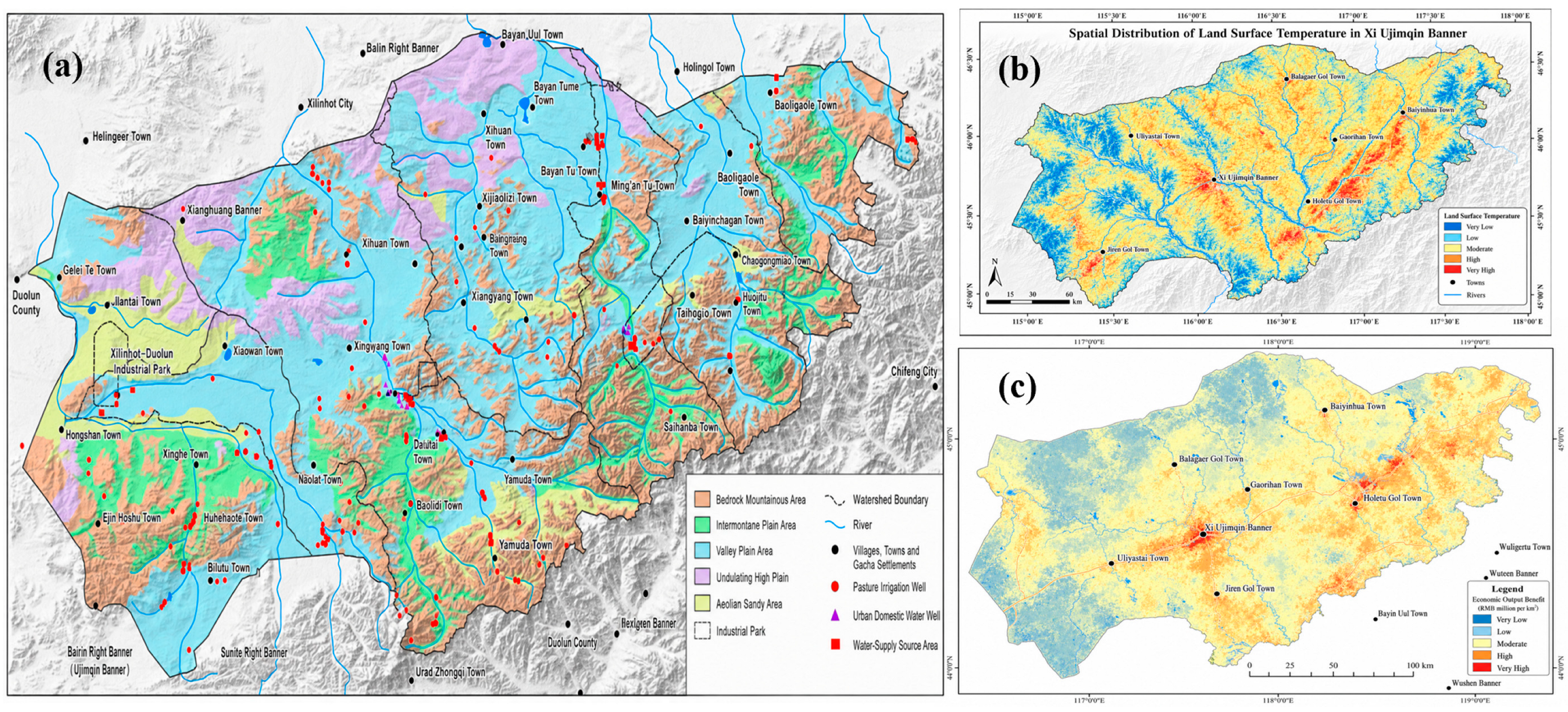
Xi Ujimqin Banner is located in the eastern part of Xilingol League, Inner Mongolia, northern China. It is a typical semi-arid grassland county-level region, with a total land area of approximately 22,434.5 km². As shown in Figure 1a, the study area has a heterogeneous geographical and geomorphological structure, including bedrock mountainous areas, intermontane plains, valley plains, undulating high plains, aeolian sandy areas, industrial parks, rivers, watershed boundaries, towns, and gacha settlements. This spatial heterogeneity provides a representative geographical basis for examining the relationships among landform conditions, remotely sensed surface thermal patterns, vegetation and bare-land distribution, SVF-based spatial openness, and land-development activities [33,34,35,36,39,40,41,42].

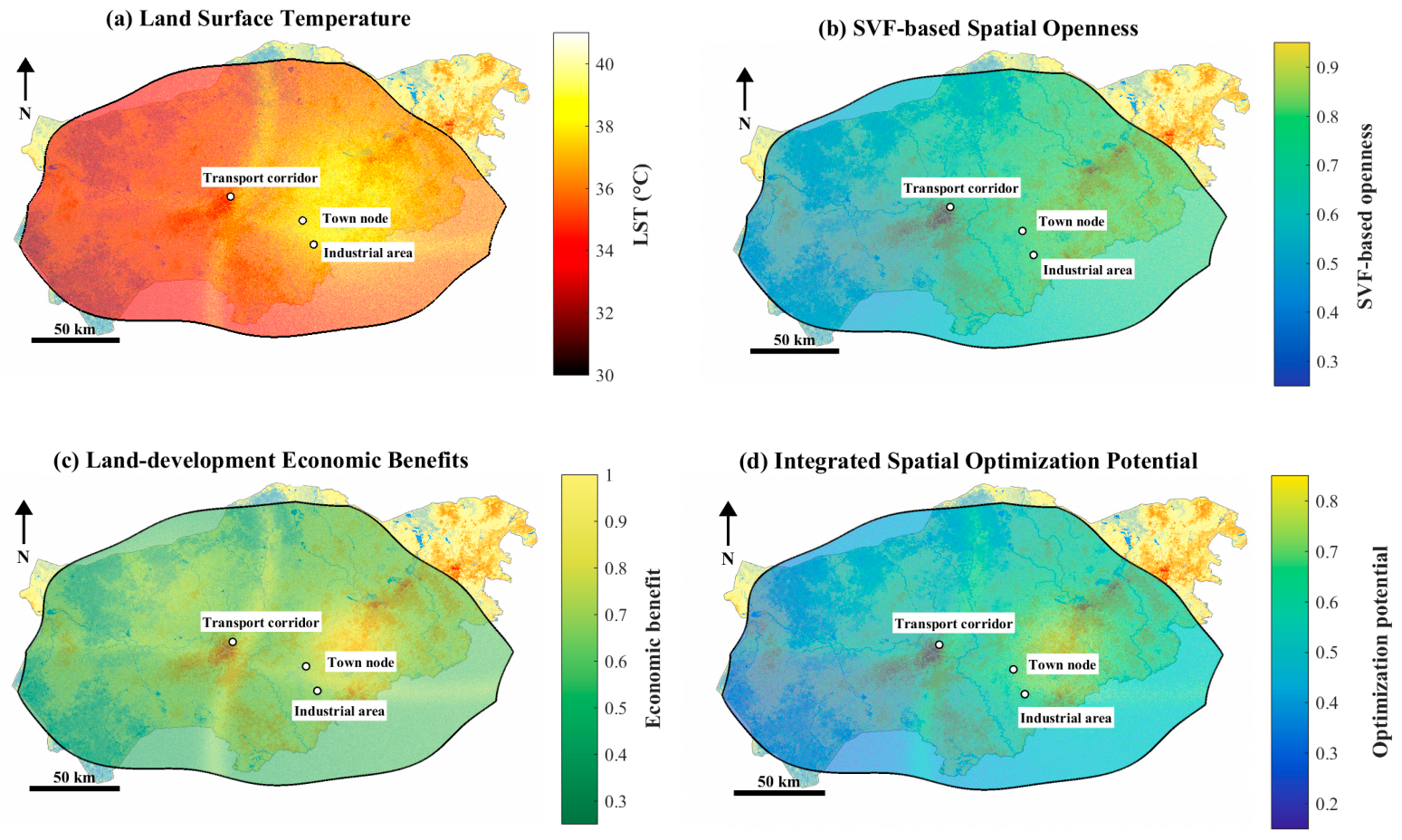
The region has a continental semi-arid climate, characterized by cold winters, hot summers, limited precipitation, strong evaporation, and relatively high wind speeds. The annual precipitation is approximately 336.5–345 mm, whereas the annual evaporation reaches about 1747.3 mm, nearly five times the annual precipitation. The terrain generally slopes from southeast to northwest, with elevations ranging from approximately 850 m to 1960 m. These climatic and topographic conditions contribute to spatial differences in vegetation coverage, bare-land exposure, LST, and heat-dissipation-related spatial conditions. As shown in Figure 1b, the remote-sensing-derived LST map indicates that higher-temperature areas are mainly distributed around built-up areas, transport corridors, industrial land, and exposed surfaces, whereas relatively low-temperature areas are mainly associated with river corridors, vegetated zones, mountainous areas, and higher-elevation areas [33,34,35,36,42].

Land use in Xi Ujimqin Banner is dominated by grassland, which accounts for approximately 85.0% of the total area, followed by unused land, forest land, construction land, cultivated land, and water/wetland areas. Vegetation coverage generally decreases from the southeast to the northwest, forming an ecological gradient that can be captured by remote-sensing-derived vegetation and land-cover indicators. Meanwhile, the banner has a resource-based economy, with coal mining, power generation, mineral processing, and related industrial activities serving as major sources of economic output. As shown in Figure 1c, land-development economic output benefits are spatially uneven, with higher values mainly concentrated around town centers, industrial areas, and major development corridors. Therefore, Xi Ujimqin Banner provides an appropriate empirical setting for examining how remote-sensing-derived surface thermal exposure, SVF-based spatial openness and heat-dissipation proxy, ecological constraints, and land-development economic benefits can be coordinated within a constrained spatial optimization framework.

2.2. Research Framework

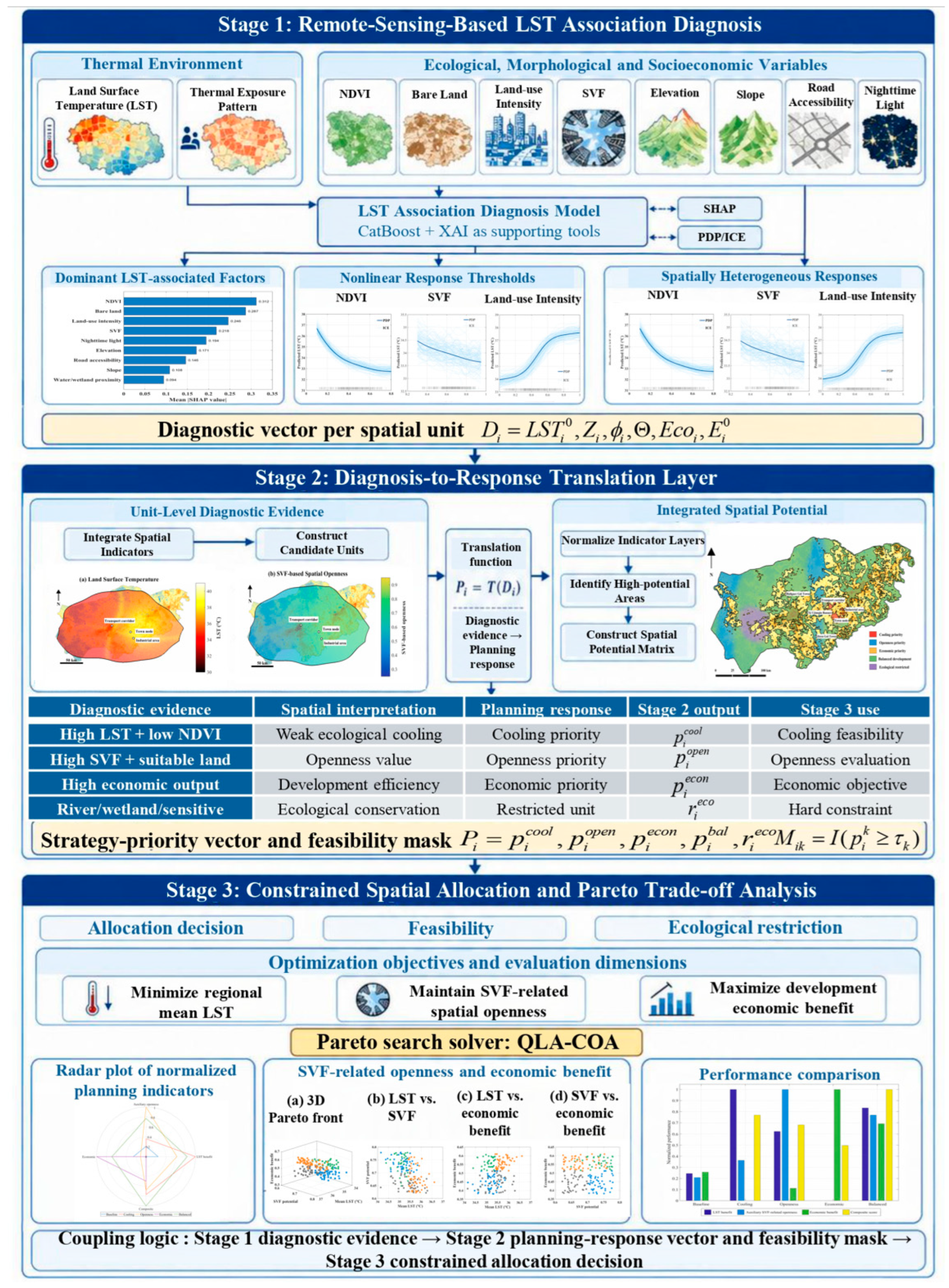
This study employed a three-stage diagnosis-to-allocation framework to support remote-sensing-informed heat-resilient spatial planning in Xi Ujimqin Banner (Figure 2). The purpose of the framework is to convert remote-sensing-based thermal-environment diagnosis into spatial allocation schemes that can support planning decisions. Specifically, the framework links three tasks: identifying model-explained LST associations, translating diagnostic information into planning-response priorities, and generating multi-objective allocation schemes under planning constraints.

To avoid treating the framework as a loose sequence of prediction, rule classification, and optimization, Stage 2 is explicitly defined as a diagnosis-to-response translation layer. In this framework, Stage 1 does not directly determine the final allocation scheme. Instead, it produces planning-relevant diagnostic information for each spatial unit. Stage 2 converts this diagnostic information into strategy-priority scores and feasibility masks, which are then incorporated into the constrained allocation model in Stage 3. Therefore, the coupling between Stage 1 and Stage 3 is established through explicit information transfer and constraint embedding. In this process, SVF-related openness is treated as a conditional spatial-form and radiative-geometry indicator, rather than as a direct cooling or actual ventilation mechanism.

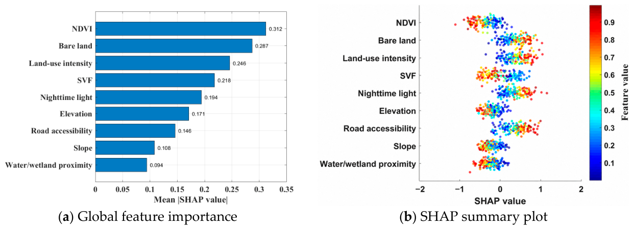
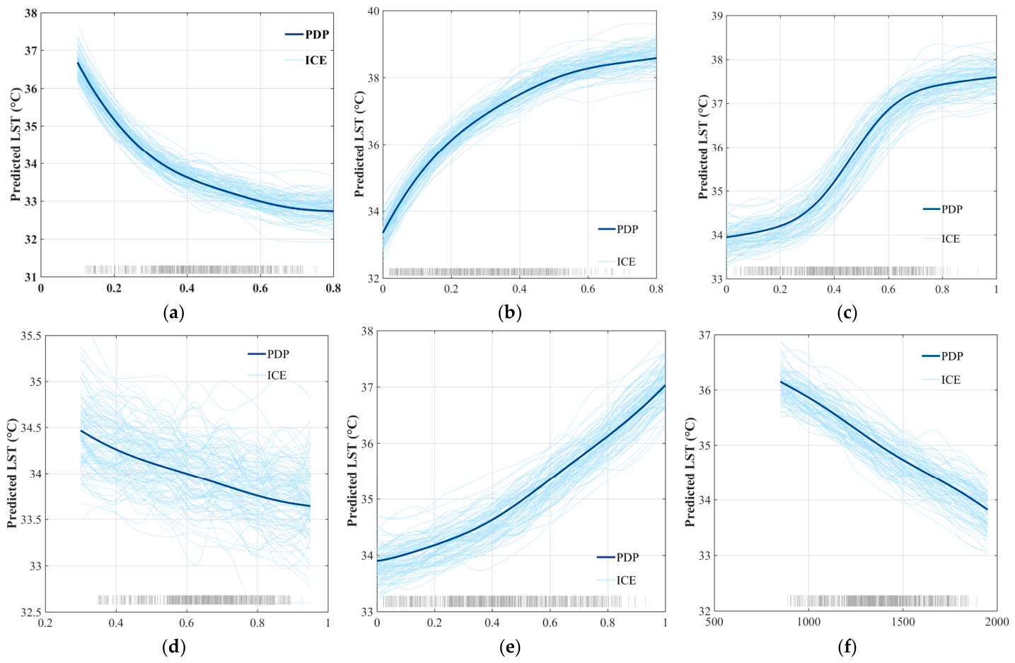
In Stage 1, remote-sensing and geospatial variables were used to construct an LST prediction and interpretation model. The dependent variable was unit-level LST, while the explanatory variables included NDVI, bare-land proportion, land-use intensity, SVF, elevation, slope, road accessibility, nighttime light intensity, and related land-use or ecological indicators. A CatBoost model was used for LST prediction, and SHAP, partial dependence plots (PDP), and individual conditional expectation (ICE) analyses were used to explain the model results. This stage identifies dominant explanatory variables, nonlinear response patterns, and spatially heterogeneous model responses associated with predicted LST. These results are interpreted as model-explained associations rather than causal effects.

For each spatial unit $i$, the diagnostic output of Stage 1 is represented as $D_i=\{LS{T}_i^0,Z_i,{\varphi }_i,\Theta ,Ec{o}_i,E_i^0\}$, where $LS{T}_i^0$ denotes the baseline LST of spatial unit $i$, $Z_i$ denotes the vector of remote-sensing, morphological, land-use, accessibility, and socioeconomic explanatory variables, ${\varphi }_i$ denotes the unit-level model-explained contribution information derived from SHAP, $\Theta$ represents nonlinear response thresholds identified from PDP/ICE interpretation, $Ec{o}_i$ denotes ecological sensitivity or restriction information, and $E_i^0$ denotes the baseline land-development economic benefit. This diagnostic vector provides the information basis for the subsequent planning-response translation.

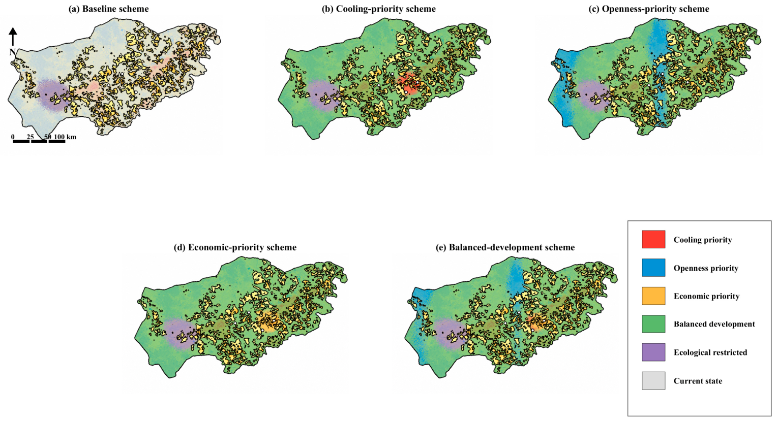
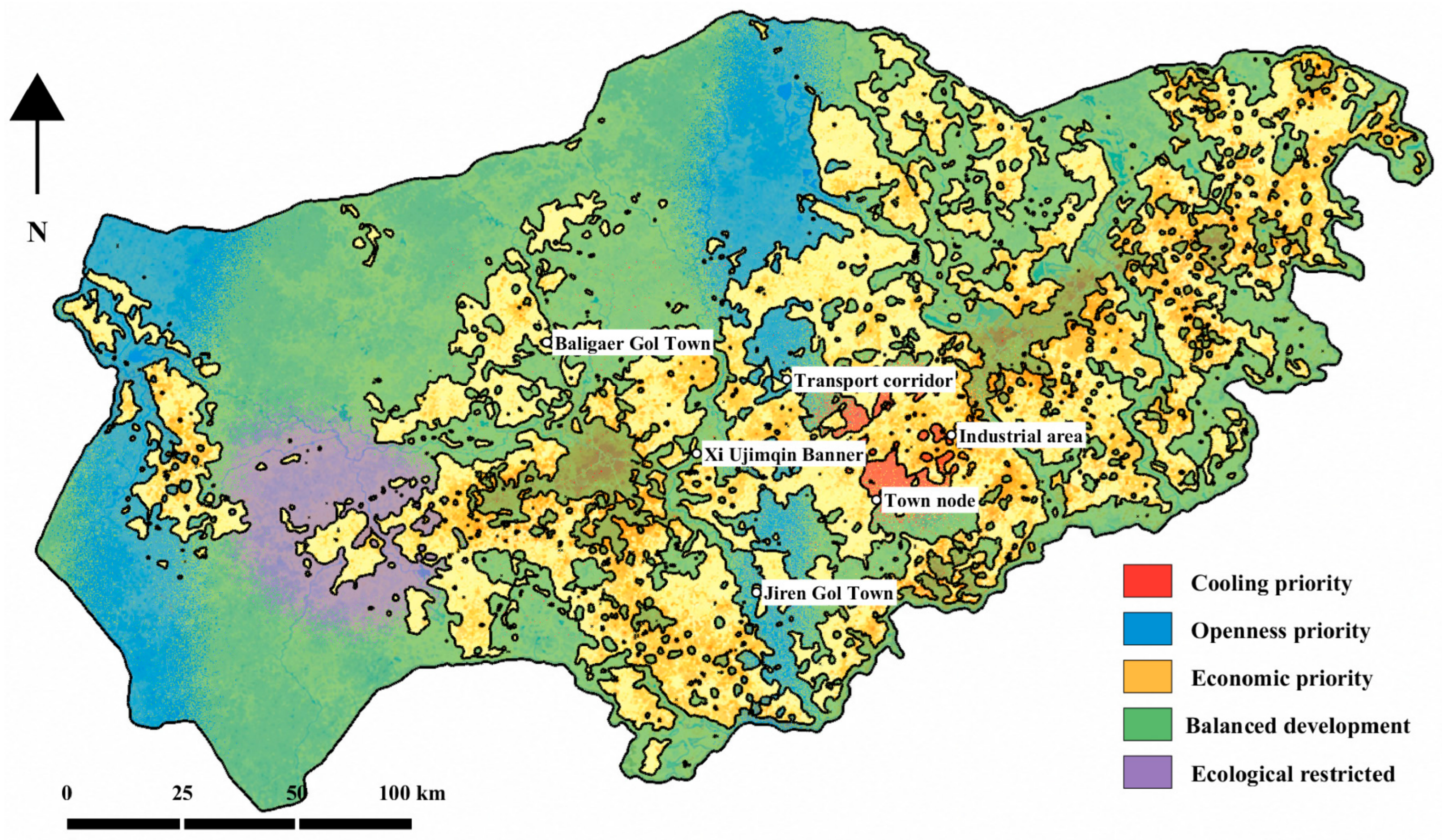
In Stage 2, the model interpretation results were translated into spatial optimization-potential categories. LST intensity, SVF-based spatial openness, land-use structure, ecological sensitivity, and land-development economic benefits were integrated at the spatial-unit level. This step classifies the study area into different planning-priority units, including cooling-priority, openness-priority, economic-priority, balanced-development, and ecological-restricted units. Here, openness-priority refers to maintaining or evaluating SVF-related spatial-form conditions, rather than simulating actual wind ventilation or assuming a direct cooling effect.

More specifically, Stage 2 converts the diagnostic vector $D_i$ into strategy-priority scores, expressed as $p_{ik}=T_k(D_i),k\in K$, where $T_k(\cdot )$ denotes the diagnosis-to-response translation function for strategy $k$, and $p_{ik}$ represents the relative planning priority or suitability of assigning spatial unit $i$ to strategy $k$. The strategy set is defined as $K=\{0,1,2,3,4\}$, where $k=0$ denotes current-state maintenance, $k=1$ denotes cooling priority, $k=2$ denotes openness priority, $k=3$ denotes economic priority, and $k=4$ denotes balanced development.

Based on the strategy-priority score, a feasibility mask is further defined as $M_{ik}=I(p_{ik}\ge {\tau }_k)$, where $M_{ik}$ indicates whether spatial unit $i$ is feasible for strategy $k$, $I(\cdot )$ is an indicator function, and ${\tau }_k$ is the minimum priority threshold for strategy $k$. Ecological-restricted units are identified using ecological sensitivity and protection information and are subsequently incorporated as hard constraints in the allocation model. In this way, Stage 2 is not a black-box empirical classification step, but a transparent translation process that converts LST-model-explained spatial patterns into optimization-ready strategy signals.

In Stage 3, a constrained multi-objective spatial allocation model was formulated to generate alternative heat-resilient planning schemes. Let $x_{ik}$ denote the binary allocation decision variable, where $x_{ik}=1$ if spatial unit $i$ is assigned to strategy $k$, and $x_{ik}=0$ otherwise. The feasibility mask derived from Stage 2 is embedded into the allocation model as $x_{ik}\le M_{ik},\forall i\in N,k\in K$. Thus, a spatial unit can only be assigned to a strategy when its diagnostic characteristics support the corresponding planning response. For ecological-restricted units, development-oriented allocation is further prohibited or limited through ecological hard constraints.

For each spatial unit $i$ and strategy $k$, the strategy-specific response values are denoted as $LS{T}_{ik}$, $SV{F}_{ik}$, and $E_{ik}$, representing the expected thermal response, SVF-based spatial openness response, and land-development economic benefit, respectively. These response values are derived from baseline spatial data, strategy-specific adjustment rules, and model-based prediction, and are then used in the objective functions of the allocation model.

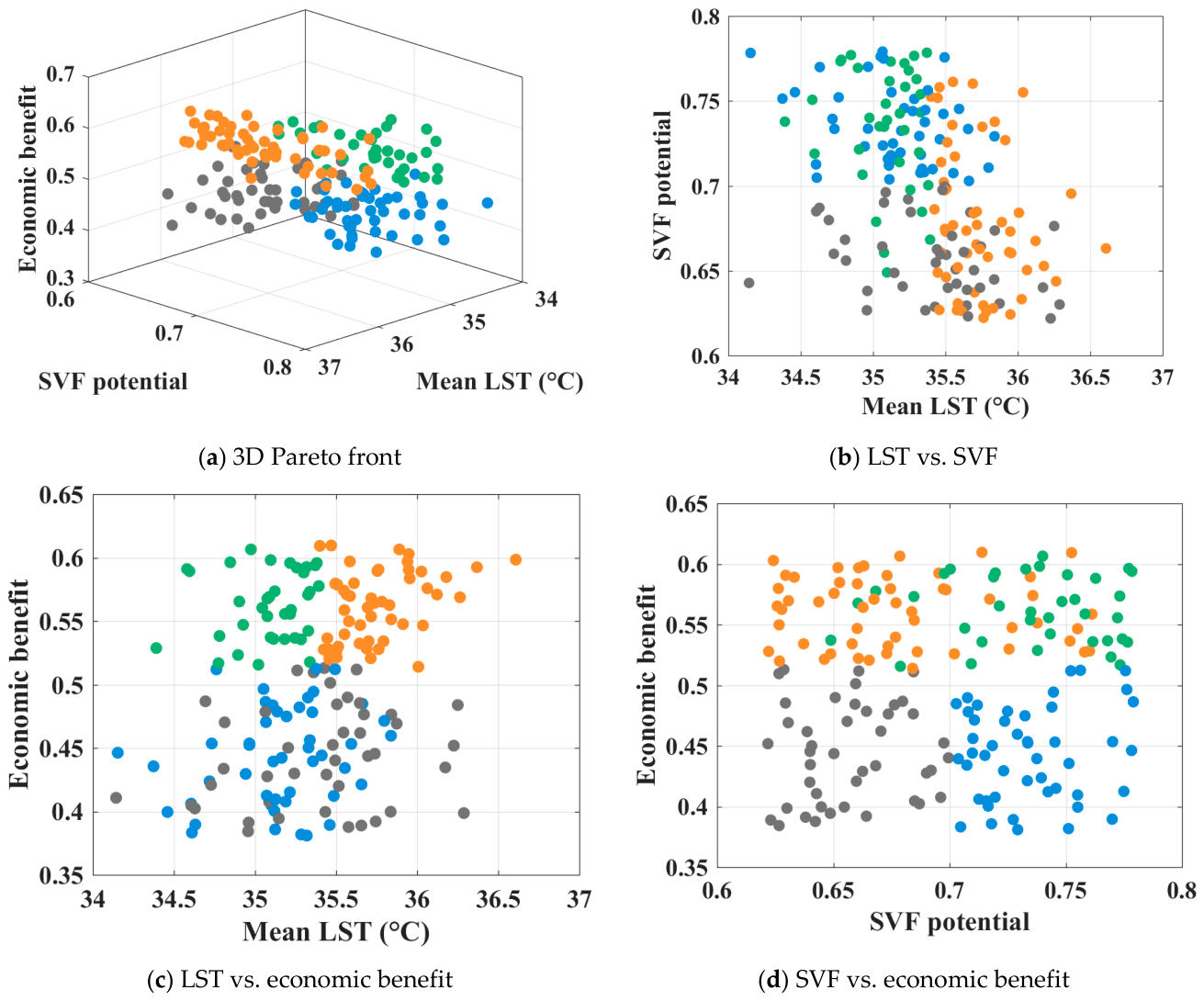
The allocation model aims to reduce regional mean LST and maintain land-development economic benefits, while considering constraints related to ecological protection, land-use suitability, spatial scale, SVF-related spatial-form conditions, and basic economic-development requirements. Therefore, LST reduction and land-development economic benefit are treated as the two primary planning objectives. SVF-related spatial openness is not treated as a direct temperature-control objective. Instead, it is retained only as an auxiliary spatial-form and radiative-geometry indicator to evaluate whether allocation schemes excessively sacrifice openness-related spatial conditions. The QLA-COA algorithm was used as a solver to search for Pareto-efficient allocation solutions under these constraints. The resulting solution set was further used to compare representative planning schemes, including cooling-priority, openness-priority, economic-priority, and balanced-development schemes.

Through this formulation, the three stages are mathematically and procedurally connected as follows: Stage 1 produces the diagnostic vector $D_i$; Stage 2 translates $D_i$ into strategy-priority scores $p_{ik}$ and feasibility masks $M_{ik}$; and Stage 3 incorporates $M_{ik}$, $x_{ik}$, and the strategy-specific response values $LS{T}_{ik}$, $SV{F}_{ik}$, and $E_{ik}$ into the constrained multi-objective allocation model. Therefore, the proposed framework is organized as a structured process of remote-sensing-based LST diagnosis $\to$ planning-response translation $\to$ constrained spatial allocation, rather than as a loosely connected technical workflow.

To avoid treating Stage 2 as an empirical black-box classification procedure,

Table 1. Diagnosis-to-response translation matrix linking LST-model-explained associations with allocation-model inputs.

Stage 1 Diagnostic Evidence	Threshold or Decision Basis	Spatial Interpretation	Stage 2 Output	Stage 3 Use	Strategy Response
Low NDVI + high LST	$NDV{I}_i\le {\theta }_{NDVI}$ and $LS{T}_i^0\ge Q_{75}(LST)$	Weak vegetation cooling and high marginal cooling potential	$p_{i1}$, $M_{i1}$	Cooling feasibility constraint	Cooling-priority/ecological restoration
High bare-land exposure + high LST	$Bar{e}_i\ge {\theta }_{Bare}$ or upper-quantile exposed-surface units	Exposed surfaces amplify surface heat accumulation	$p_{i1}$, $M_{i1}$	Cooling and restoration feasibility	Cooling-priority/ecological buffering
High land-use intensity	$LU{I}_i\ge {\theta }_{LUI}$ and $Ec{o}_i=0$	Development intensity may increase thermal pressure	$p_{i4}$, $M_{i4}$	Balanced allocation with thermal-risk control	Balanced development
High SVF + suitable land condition	$SV{F}_i\ge {\theta }_{SVF}$ and $Ec{o}_i=0$	SVF-based openness has heat-dissipation planning value	$p_{i2}$, $M_{i2}$	Openness-related evaluation or constraint	Openness priority
High nighttime light/economic output	$NT{L}_i\ge {\theta }_{NTL}$ or $E_i^0\ge Q_{75}(E)$, and $Ec{o}_i=0$	Economic activity overlaps with thermal pressure	$p_{i3}$, $M_{i3}$	Economic-benefit objective with LST constraint	Economic priority/balanced development
River, wetland, or ecological-sensitive unit	$Ec{o}_i=1$	Ecological conservation and cooling-retention function should be prioritized	$r_i^{eco}=1$	Hard constraint on development-oriented allocation	Ecological restricted

is a diagnosis-to-response translation matrix. The purpose of this matrix is not to impose arbitrary planning rules, but to convert the LST-model-explained associations identified in Stage 1 into explicit strategy-priority scores and feasibility masks for Stage 3. For each spatial unit $i$, the diagnostic information is summarized as $D_i=LS{T}_i^0,Zi,\varphi i,\Theta ,Ec{o}_i,E_i^0$. Stage 2 translates $D_i$ into strategy-priority scores $pik=T_k(D_i)$, where $k$ denotes the candidate planning strategy. A feasibility mask is then defined as $Mik=I(p_{ik}\ge {\tau }_k)$ and embedded into the allocation model through the constraint $x_{ik}\le M_{ik}$. Therefore, the Stage 2 classification is not an isolated empirical rule set, but an explicit information-transfer layer connecting LST diagnosis with constrained spatial allocation.

Through this translation matrix, the Stage 2 classification is no longer an isolated empirical rule set. Instead, it provides optimization-ready inputs for Stage 3 by converting diagnostic evidence into strategy-priority scores $p_{ik}$, feasibility masks $M_{ik}$, and ecological restriction indicators $r_i^{eco}$. The resulting information-transfer chain can be summarized as $D_i\to p_{ik}\to M_{ik}\to x_{ik}$. This design explicitly connects model-explained LST associations with constrained spatial allocation decisions.

2.3. Metrics and Data Sources

As illustrated in Figure 2, the proposed framework consists of three progressive stages: LST association diagnosis, spatial optimization-potential assessment, and constrained spatial allocation optimization. To support these stages, this study constructed two primary optimization indicators and one auxiliary spatial-form indicator. The two primary indicators were land surface temperature (LST) and land-development economic output benefits, while SVF-related spatial openness was used as an auxiliary spatial-form and radiative-geometry indicator. These indicators were first used to characterize the spatial conditions of Xi Ujimqin Banner. In the allocation model, LST reduction and land-development economic benefit were incorporated as the two primary optimization objectives, whereas SVF-related spatial openness was used only for auxiliary evaluation and constraint-related planning assessment rather than as a direct temperature-control objective. In addition, a set of explanatory variables was constructed to identify the nonlinear model-explained associations of LST using interpretable machine learning.

To support the proposed heat-resilient spatial allocation framework, this study integrated multi-source spatial, environmental, and socioeconomic datasets. Landsat 8/9 Collection 2 Level-2 infrared data were used to characterize surface thermal exposure. DEM/DSM and morphology-related data were used to evaluate SVF-related spatial openness, which was interpreted as a county-scale spatial-form and radiative-geometry indicator rather than as a direct measure of actual ventilation capacity. Land-use and socioeconomic datasets were used to characterize land-use structure, ecological constraints, accessibility, and land-development economic output benefits. River corridors, wetlands, water bodies, and ecological protection data were further used to construct the ecological-restricted constraint layer in the spatial allocation model.

Table 2. Main datasets and analytical roles in this study.

Data Category	Data Source	Main Variables	Analytical Role
Thermal remote sensing	Landsat 8/9 Collection 2 Level-2 Surface Temperature	LST	Thermal exposure assessment and primary LST-reduction objective
Multispectral remote sensing	Landsat 8/9 Collection 2 Level-2 Surface Reflectance	NDVI, vegetation condition, surface exposure	LST association diagnosis and vegetation/exposure-related planning signals
Terrain and morphology	DSM/DEM-derived terrain and openness layers	Elevation, slope, SVF-related spatial openness	Terrain background analysis and auxiliary spatial-form/radiative-geometry evaluation
Land-use/land-cover	ESA WorldCover and local land-use data	Grassland, construction land, bare land, forest, water/wetland	Land-use structure identification, strategy feasibility, and ecological/background interpretation
Socioeconomic and accessibility data	VIIRS nighttime light, GDP, roads, industrial land	Nighttime light, economic output, road accessibility	Economic-benefit estimation and primary land-development economic objective
Ecological constraint data	River/wetland layers, ecological-sensitive zones, monitoring locations	River corridors, wetlands, water bodies, ecological-sensitive areas	Ecological-restricted constraint layer and hard ecological protection boundary

Note: SVF-related spatial openness was used as an auxiliary spatial-form and radiative-geometry indicator rather than as a direct ventilation, cooling, or temperature-control objective. The two primary optimization objectives were LST reduction and land-development economic benefit.

shows the main datasets and analytical roles in this study.

2.3.1. Remote Sensing Data Acquisition and Preprocessing

To improve the reproducibility of the remote-sensing-based analysis, the data acquisition and preprocessing procedures were further specified. Landsat thermal infrared data were used to derive land surface temperature (LST), while Landsat multispectral bands were used to calculate vegetation and surface-exposure indicators. Warm-season images were selected to represent typical surface thermal conditions in Xi Ujimqin Banner. Images with excessive cloud contamination over the study area were excluded. Cloud, cloud-shadow, snow, and invalid pixels were removed using the quality-assessment band provided with the Landsat product. Water-dominated pixels were masked when calculating terrestrial LST statistics to avoid bias caused by water-surface thermal properties.

All raster datasets, including LST, NDVI, land-use/land-cover data, DEM/DSM-derived terrain and morphology indicators, nighttime light data, road-accessibility indicators, and ecological constraint layers, were projected to a unified coordinate system before spatial analysis. Continuous variables, such as LST, NDVI, elevation, slope, SVF-related spatial openness, nighttime light intensity, and accessibility indicators, were resampled using bilinear interpolation, whereas categorical land-use data were resampled using nearest-neighbor assignment. After preprocessing, all raster variables were aggregated to the same spatial analysis units using zonal statistics. The mean values of continuous variables and the area proportions of categorical land-use types were calculated for each spatial unit. These harmonized spatial variables were then used for LST association diagnosis, spatial optimization-potential assessment, and constrained spatial allocation optimization.

A detailed list of remote sensing datasets, product names, acquisition dates, spatial resolutions, cloud-screening criteria, preprocessing steps, and their roles in the analysis is provided in Appendix A.1 

Table A1. Partial sample of SVF-related spatial-unit records used for reproducibility checking.

Unit ID	DSM Product	Resolution	Search Radius	Directions	Mean Elevation	SVF-Related Openness	LST	NDVI	Bare-Land Proportion	Eco-Restricted	${\mathit{p}}_{\mathit{i}2}^{\mathit{o}\mathit{p}\mathit{e}\mathit{n}}$	${\mathit{M}}_{\mathit{i}2}$
0001	Copernicus DEM GLO-30 DSM	30 m	$R=300$	$n=36$	1028.4	0.842	32.18	0.41	0.18	0	0.76	1
0002	Copernicus DEM GLO-30 DSM	30 m	$R=300$	$n=36$	1046.7	0.801	33.05	0.36	0.24	0	0.69	1
0003	Copernicus DEM GLO-30 DSM	30 m	$R=300$	$n=36$	978.2	0.756	34.62	0.28	0.35	0	0.58	1
0004	Copernicus DEM GLO-30 DSM	30 m	$R=300$	$n=36$	1102.5	0.887	30.74	0.53	0.09	1	0.31	0
0005	Copernicus DEM GLO-30 DSM	30 m	$R=300$	$n=36$	1065.9	0.829	31.46	0.47	0.14	0	0.73	1
0006	Copernicus DEM GLO-30 DSM	30 m	$R=300$	$n=36$	995.6	0.713	35.08	0.22	0.42	0	0.49	0
0007	Copernicus DEM GLO-30 DSM	30 m	$R=300$	$n=36$	1017.3	0.865	32.67	0.39	0.21	0	0.78	1
0008	Copernicus DEM GLO-30 DSM	30 m	$R=300$	$n=36$	1088.1	0.792	31.92	0.51	0.11	1	0.35	0
0009	Copernicus DEM GLO-30 DSM	30 m	$R=300$	$n=36$	963.4	0.681	36.21	0.19	0.48	0	0.42	0
0010	Copernicus DEM GLO-30 DSM	30 m	$R=300$	$n=36$	1039.8	0.818	33.27	0.34	0.27	0	0.66	1
…
1531	Copernicus DEM GLO-30 DSM	30 m	$R=300$	$n=36$	1215.6	0.884	37.94	0.22	0.60	0	0.76	1

.

2.3.2. Land Surface Temperature

LST was used to represent the spatial intensity of surface thermal exposure. In this study, LST was derived from Landsat thermal infrared data, which are widely used for urban and regional thermal-environment analysis because of their relatively high spatial resolution and long-term availability. To capture warm-season thermal characteristics, cloud-free images during the growing season or summer period were selected for LST retrieval or directly obtained from standard surface temperature products [1,2,3,4].

After preprocessing, invalid pixels, water-dominated pixels, and cloud-contaminated areas were removed. The valid LST pixels were then aggregated to the spatial analysis units by calculating the mean value. LST was used not only as the dependent variable in the interpretable machine learning model, but also as the first optimization objective. The regional mean LST was minimized as follows:

$$\min F_1={\displaystyle \frac{1}{N}}{\displaystyle \sum _{i=1}^{N}L}S{T}_i,$$

(1)

where $LS{T}_i$ denotes the mean land surface temperature of spatial unit $i$, and $N$ denotes the total number of spatial units. A lower value of $F_1$ indicates better overall surface thermal mitigation performance.

2.3.3. SVF-Based Spatial Openness and Heat-Dissipation Proxy

The sky view factor (SVF) was used to characterize spatial openness and radiative-geometry-related heat-dissipation conditions. SVF reflects the proportion of visible sky from a given surface location and is closely associated with terrain openness, surface geometry, radiative heat exchange, and the potential release of accumulated heat [25]. Previous studies have widely used SVF as a morphological and radiative-geometry indicator in urban thermal-environment research, including studies of land surface temperature, urban heat island intensity, radiation-related thermal comfort, and heat-sensitive urban design [26]. However, SVF was not treated in this study as a direct measure of actual ventilation capacity or as an independent causal cooling indicator. True ventilation potential depends on additional meteorological and morphological factors, including wind direction, wind speed, surface roughness, topographic channels, building resistance, and corridor connectivity.

To improve the transparency and reproducibility of the SVF-related calculation, the data source and calculation parameters were further specified. The SVF-related spatial openness layer was derived from the Copernicus DEM GLO-30 product. Although this product is named as a DEM, Copernicus DEM is officially described as a Digital Surface Model (DSM) representing the top-reflective surface of the Earth, including buildings, infrastructure, and vegetation where represented in the product. Therefore, it was used as the surface-height input for county-scale SVF-related openness calculation. Before calculation, the DSM was projected to the same coordinate system as the other raster layers, checked for void values, resampled to the common analysis resolution, and clipped to the study boundary.

SVF-related openness was calculated using a ray-tracing or horizon-angle-based approach. The maximum search radius was set to $R$ m, and the number of azimuth calculation directions was set to $n$. These two parameters control the spatial extent and directional resolution of surrounding obstruction detection. The pixel-level SVF-related openness values were then aggregated to spatial analysis units using zonal statistics. The DSM source, spatial resolution, preprocessing steps, maximum search radius, number of azimuth directions, and aggregation procedure are reported in Appendix A.1 Table A1.

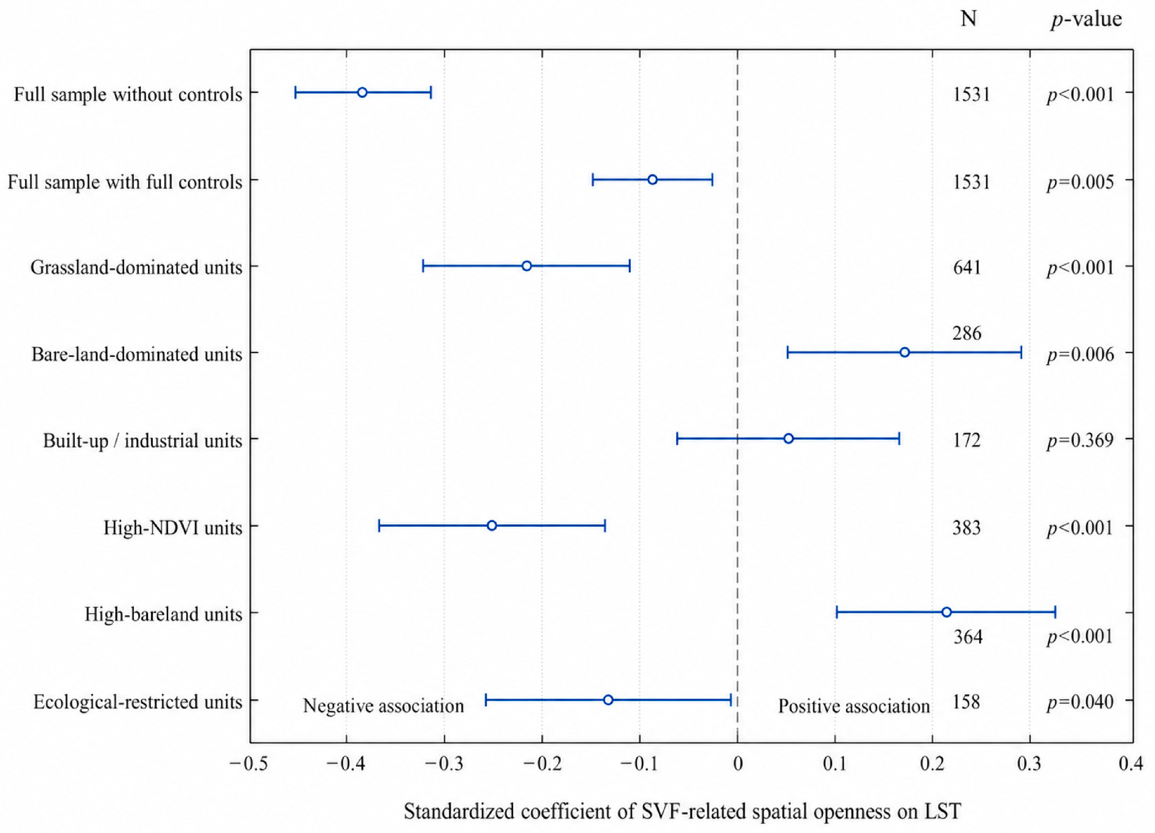
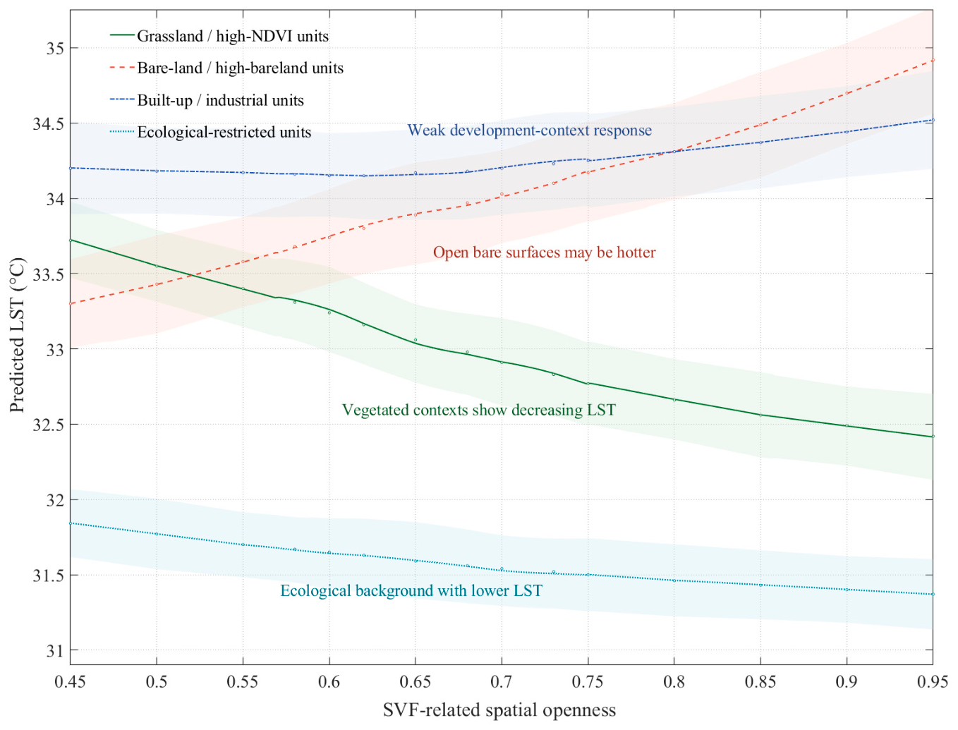
This distinction is particularly important in semi-arid grassland towns such as Xi Ujimqin Banner. In such regions, high SVF may indicate stronger spatial openness and lower physical obstruction, which can support longwave heat release under certain conditions [31,32]. However, high SVF may also correspond to limited shading, stronger daytime solar radiation exposure, and bare-land surfaces, which do not necessarily lead to daytime cooling. Therefore, the SVF-based indicator was interpreted together with LST, NDVI, bare-land proportion, land-use intensity, and ecological background conditions, rather than being interpreted as a standalone cooling or ventilation indicator.

Because the spatial resolution of Copernicus DEM GLO-30 is approximately 30 m, the derived indicator should be interpreted as a county-scale SVF-related spatial openness indicator rather than a fine-scale street-canyon, building-shading, or tree-canopy microclimate variable. It can reflect broad spatial openness and surface-geometry conditions at the regional planning scale, but it cannot replace field-based microclimate observations or high-resolution urban canopy modeling.

As shown in Stage 2 and Stage 3 of Figure 2, the SVF-based indicator was used as an auxiliary spatial-form indicator for assessing optimization potential and for evaluating allocation schemes. In the optimization framework, LST reduction and land-development economic benefit were treated as the two primary planning objectives, while SVF-based spatial openness was incorporated as an auxiliary planning dimension. Its role was to prevent allocation schemes from excessively sacrificing openness-related heat-release conditions, rather than to serve as an independent temperature-control objective. The area-weighted mean SVF-based spatial openness indicator was calculated as follows:

$$F_{\mathrm{SVF}}={\displaystyle \frac{{\displaystyle \sum _{i=1}^N{A}_i}SV{F}_i}{{\displaystyle \sum _{i=1}^N{A}_i}}}$$

(2)

where $SV{F}_i$ denotes the SVF-related spatial openness value of spatial unit $i$, $A_i$ denotes the area of spatial unit $i$, and $N$ denotes the total number of spatial units. A higher value of $F_{\mathrm{SVF}}$ indicates stronger county-scale spatial openness. However, $F_{\mathrm{SVF}}$ does not directly represent actual ventilation capacity or causal cooling potential. In this study, $F_{\mathrm{SVF}}$ was used only as an auxiliary evaluation indicator and constraint-related planning proxy, rather than as an independent thermal objective equivalent to LST reduction.

2.3.4. Land-Development Economic Output Benefits

Land-development economic output benefits were used to represent the spatial economic efficiency of development-oriented land use. To improve the transparency and reproducibility of this indicator, this study spatialized economic benefits using a calibrated proxy-based allocation model rather than a simple qualitative assignment. Specifically, township-level economic statistics were allocated to spatial analysis units by integrating nighttime light intensity, construction-land proportion, industrial-land proportion, and road accessibility. These variables were selected because nighttime light intensity reflects the intensity of socioeconomic activity, construction land represents the spatial basis of development, industrial land indicates production-oriented economic activity, and road accessibility reflects the locational advantage of land development.

First, all proxy variables were normalized using min--max normalization: $X_{i,m}^{\prime }={\displaystyle \frac{X_{i,m}-\min (X_m)}{\max (X_m)-\min (X_m)}},$ where $X_{i,m}^{\prime }$ denotes the normalized value of proxy variable $m$ in spatial unit $i$. The proxy variables included normalized nighttime light intensity $(NT{L}_i^{\prime })$, construction-land proportion $(C{L}_i^{\prime })$, industrial-land proportion $(I{L}_i^{\prime })$, and road accessibility $(R{A}_i^{\prime })$. A composite economic-development suitability score was then calculated as: $S_i=w_{1}NT{L}_i^{\prime }+w_{2}C{L}_i^{\prime }+w_{3}I{L}_i^{\prime }+w_{4}R{A}_i^{\prime },$ where $S_i$ represents the economic-development suitability score of spatial unit $i$, and $w_1$, $w_2$, $w_3$, and $w_4$ are the weights of nighttime light intensity, construction-land proportion, industrial-land proportion, and road accessibility, respectively. The weights were estimated through calibration against available township-level economic statistics under the following constraints: $w_m\ge 0,\hspace{1em}{\displaystyle \sum _{m=1}^4{w}_m}=1$. The calibrated weights are reported in Appendix A.2 

Table A2. Proxy-based calibration and diagnostic results of economic-benefit spatialization.

Component	Indicator	Estimated Value	Interpretation
Weighting scheme	Nighttime light intensity weight (w_1)	0.36	Main proxy for socioeconomic activity
Weighting scheme	Construction-land proportion weight (w_2)	0.24	Proxy for development land base
Weighting scheme	Industrial-land proportion weight (w_3)	0.27	Proxy for production-oriented economic activity
Weighting scheme	Road accessibility weight (w_4)	0.13	Proxy for locational accessibility
Calibration accuracy	(R^2) between estimated and observed township economic output	0.84	Good consistency with township-level statistics
Calibration accuracy	MAE	0.064	Low average normalized error
Calibration accuracy	RMSE	0.087	Acceptable normalized prediction error
Calibration accuracy	MAPE	12.6%	Acceptable relative error for spatial proxy estimation
Diagnostic correlation	Economic-benefit layer vs. nighttime light intensity	(r = 0.76, p < 0.001)	Strong positive association
Diagnostic correlation	Economic-benefit layer vs. construction-land proportion	(r = 0.68, p < 0.001)	Moderate-to-strong positive association
Diagnostic correlation	Economic-benefit layer vs. industrial-land proportion	(r = 0.72, p < 0.001)	Strong positive association
Diagnostic correlation	Economic-benefit layer vs. road accessibility	(r = 0.51, p < 0.001)	Moderate positive association
Trade-off diagnosis	Economic benefit vs. LST	(r = 0.58, p < 0.001)	Economically intensive areas tend to show higher LST
Trade-off diagnosis	Economic benefit vs. SVF-based openness	(r = −0.32, p = 0.004)	Intensive development may partly conflict with spatial openness

. For each township $g$, the observed economic output $GD{P}_g$ was spatially allocated to its internal spatial units according to the weighted suitability score and development-land area: $GD{P}_i=GD{P}_g\times {\displaystyle \frac{S_i{A}_i^{dev}}{{\displaystyle \sum _{j\in g}{S}_j}{A}_j^{dev}+\epsilon }},$ where $GD{P}_i$ denotes the estimated economic output of spatial unit $i$, $A_i^{dev}$ denotes the development or construction land area of unit $i$, and $\epsilon$ is a small constant used to avoid division by zero. The land-development economic output benefit of each unit was then calculated as: $E_i={\displaystyle \frac{GD{P}_i}{A_i^{dev}+\epsilon }},$ where $E_i$ represents the estimated economic output per unit development land area. A higher value of $E_i$ indicates stronger land-development economic efficiency.

To evaluate the credibility of the spatialization result, the estimated unit-level economic outputs were aggregated back to township units and compared with observed township-level economic statistics. The calibration accuracy was assessed using $R^2$, mean absolute error (MAE), root mean square error (RMSE), and mean absolute percentage error (MAPE). In addition, diagnostic correlation analysis was conducted between the spatialized economic-benefit layer and its major proxy variables, including nighttime light intensity, construction-land proportion, industrial-land proportion, and road accessibility. Pearson and Spearman correlation coefficients were calculated to examine whether the spatialized economic-benefit pattern was consistent with the expected socioeconomic and land-development structure.

The resulting economic-benefit layer was used in two ways. First, it was used to identify economic-priority and balanced-development units in the spatial optimization-potential assessment. Second, it was incorporated into the multi-objective allocation model as the third optimization objective and as part of the minimum economic-development constraint. Development-oriented allocation was prohibited in ecological-restricted units, and economic-priority strategies were evaluated only within units satisfying land-use suitability and ecological constraint conditions.

$$\max F_2={\displaystyle \sum _{i=1}^N\frac{GD{P}_i}{A_i^{dev}}},$$

(3)

where $GD{P}_i$ denotes the estimated economic output of spatial unit $i$, and $A_i^{dev}$ denotes the area of development land or construction land within spatial unit $i$. A higher value of $F_2$ indicates stronger land-development economic efficiency. For Xi Ujimqin Banner, areas around town centers, industrial parks, mining areas, transportation corridors, and major development zones generally show higher economic output benefits, whereas grassland-dominated and ecologically sensitive areas show relatively lower development intensity.

2.3.5. Explanatory Variables for LST Mechanism Identification

In addition to the three optimization objectives, this study constructed a set of explanatory variables to identify the model-explained associations of LST. These variables included ecological indicators, morphological indicators, land-use indicators, accessibility indicators, and socioeconomic indicators. Ecological indicators mainly included NDVI, vegetation coverage, bare-land proportion, and water/wetland distribution derived from land-use and ecological protection layers. Morphological and terrain indicators included elevation, slope, SVF, and built-up intensity. Land-use indicators described the proportions of grassland, construction land, industrial land, unused land, forest land, and water/wetland areas. Accessibility and socioeconomic indicators included road density, distance to major roads, nighttime light intensity, and estimated economic output [17,18,19,20,21,22,23,43,44,45,46].

Table 3. Candidate allocation strategies used in the spatial optimization model.

Strategy Code	Strategy Type	Main Planning Orientation	Expected Spatial Response
(k = 0)	Current-state maintenance	Maintain existing land-use condition	No major change in LST, SVF, or economic benefit
(k = 1)	Cooling-priority strategy	Reduce surface thermal exposure	Lower LST, improved ecological cooling
(k = 2)	Ventilation-priority strategy	Enhance openness and heat dissipation	Higher SVF-based ventilation potential
(k = 3)	Economic-efficiency-priority strategy	Improve land-development output	Higher economic benefit, possible thermal trade-off
(k = 4)	Balanced-development strategy	Coordinate thermal, ventilation, and economic objectives	Moderate improvement across multiple objectives

summarizes the planning orientation and expected spatial response of each strategy.

These variables were used as input features for the interpretable machine learning model in Stage 1 of Figure 2. By analyzing feature importance, marginal effects, and nonlinear responses, the model provided a mechanism-based explanation of spatial LST differentiation and supported the subsequent spatial optimization-potential assessment. The above indicators provide the data basis for the subsequent constrained multi-objective spatial allocation model. Specifically, LST, SVF-based ventilation and heat-dissipation potential, and land-development economic output benefits were used as the three optimization objectives, while ecological protection, land-use suitability, spatial scale, and development requirements were incorporated as planning constraints.

2.3.6. Machine Learning Model Training and Validation

After harmonizing all remote-sensing, morphological, land-use, accessibility, and socioeconomic variables to the same spatial analysis units, a machine learning dataset was constructed for LST mechanism identification. Each spatial unit was treated as one sample. According to the spatial optimization-potential classification, the study area contained 1531 spatial analysis units in total. For each unit, the mean LST was used as the dependent variable, while NDVI, bare-land proportion, land-use intensity, SVF, elevation, slope, road accessibility, nighttime light intensity, and water/wetland proximity were used as explanatory variables.

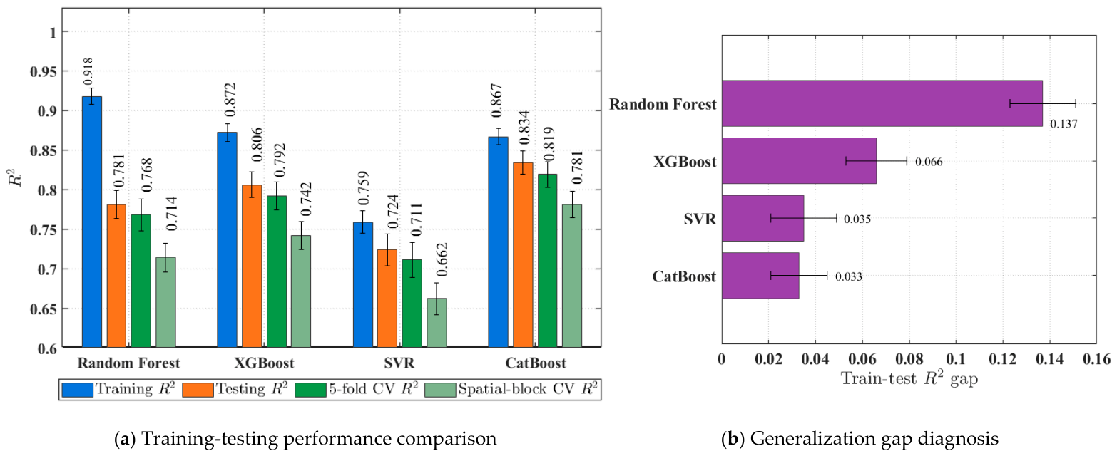
To evaluate predictive performance, the dataset was divided into training and testing subsets using an 80:20 split. The training subset was used for model fitting and hyperparameter tuning, while the testing subset was used for independent performance evaluation. To reduce the influence of random partitioning, five-fold cross-validation was further conducted on the training subset. The candidate models included Random Forest, XGBoost, Support Vector Regression, and CatBoost. Hyperparameters were optimized using grid search or randomized search within the cross-validation procedure. The final model was selected based on the testing-set performance and cross-validation stability, using R², RMSE, and MAE as evaluation metrics.

Because spatial samples may not be statistically independent, an additional spatial robustness check was conducted. The study area was divided into spatial blocks according to geographical location, and spatial block cross-validation was used to evaluate whether the model performance remained stable under spatially separated training and validation subsets. In addition, Moran’s I was calculated for the prediction residuals of the final CatBoost model to examine whether strong residual spatial autocorrelation remained. These procedures were used to reduce the risk that the reported model performance was driven only by spatially clustered samples.

2.4. Heat-Resilient Multi-Objective Spatial Allocation Model

Based on the indicators and spatial potential assessment described above, this study formulates heat-resilient spatial allocation as a constrained multi-objective optimization problem. Different from simple spatial suitability evaluation or priority ranking, the proposed model aims to determine the optimal allocation strategy for each spatial unit under multiple planning objectives. Specifically, the model seeks to generate spatial allocation schemes that can simultaneously reduce regional surface thermal exposure, enhance SVF-based ventilation and heat-dissipation potential, and maintain land-development economic output benefits. This formulation provides the mathematical basis for the subsequent QLA-COA-based optimization procedure [47,48].

2.4.1. Spatial Units and Candidate Allocation Strategies

Let $I=\{1,2,\dots ,N\}$ denote the set of spatial analysis units in Xi Ujimqin Banner, where each unit $i$ represents a grid cell, planning unit, or spatial evaluation unit. Each unit is characterized by its area $A_i$, baseline land surface temperature $LS{T}_i^0$, baseline SVF-based ventilation and heat-dissipation potential $SV{F}_i^0$, and baseline land-development economic output benefit $E{B}_i^0$.To reflect different planning preferences, this study defines a set of candidate allocation strategies: $K=\{0,1,2,3,4\},$ where $k=0$ denotes the current-state maintenance strategy, $k=1$ denotes the cooling-priority strategy, $k=2$ denotes the ventilation-priority strategy, $k=3$ denotes the economic-efficiency-priority strategy, and $k=4$ denotes the balanced-development strategy. A binary decision variable $x_{i,k}$ is introduced to describe whether spatial unit $i$ is assigned to strategy $k$:

$$x_{i,k}=\left\{\begin{array}{l}1, \mathrm{if} \mathrm{spatial} \mathrm{unit} i \mathrm{is} \mathrm{assigned} \mathrm{to} \mathrm{strategy} k,\\ 0, \mathrm{otherwise}\end{array}\right.$$

(4)

For each spatial unit, only one allocation strategy can be selected:

$${\displaystyle \sum _{k\in K}{x}_{i,k}}=1,\hspace{1em}\forall i\in I.$$

(5)

Under strategy $k$, the expected responses of spatial unit $i$ are denoted as $LS{T}_{i,k}$, $SV{F}_{i,k}$, and $E{B}_{i,k}$, representing the predicted land surface temperature, SVF-based ventilation and heat-dissipation potential, and land-development economic output benefit, respectively. These response values are derived from the spatial potential assessment and the interpretable LST mechanism model established in the previous stages.

2.4.2. Objective Functions

The heat-resilient spatial allocation model was formulated with two primary optimization objectives and one auxiliary spatial-form evaluation indicator. The two primary objectives correspond to regional LST reduction and land-development economic benefit. SVF-related spatial openness was not treated as a direct temperature-control objective. Instead, it was incorporated as an auxiliary spatial-form and radiative-geometry indicator to evaluate whether allocation schemes excessively sacrifice openness-related spatial conditions.

(1) Minimization of regional mean LST

The first objective is to reduce regional surface thermal exposure by minimizing the area-weighted mean LST after spatial allocation:

$$\min F_1(x)={\displaystyle \frac{1}{A_{\mathrm{tot}}}}{\displaystyle \sum _{i\in I}{\displaystyle \sum _{k\in K}{x}_{i,k}}}{A}_{i}LS{T}_{i,k},$$

(6)

where $A_{\mathrm{tot}}={\displaystyle \sum _{i\in I}{A}_i}$ denotes the total area of all spatial units. A lower value of $F_1(x)$ indicates better regional surface-temperature reduction performance.

(2) Maximization of land-development economic output benefits

The second primary objective is to maintain and improve land-development economic efficiency:

$$\max F_2(x)={\displaystyle \frac{1}{A_{\mathrm{dev}}}}{\displaystyle \sum _{i\in I}{\displaystyle \sum _{k\in K}{x}_{i,k}}}{A}_{i}E{B}_{i,k},$$

(7)

where $E{B}_{i,k}$ denotes the land-development economic output benefit of spatial unit $i$ under strategy $k$, and $A_{\mathrm{dev}}$ denotes the total developable land area. A higher value of $F_2(x)$ indicates stronger land-development economic efficiency.

(3) Auxiliary SVF-related spatial-form evaluation indicator

SVF-related spatial openness was calculated as an auxiliary evaluation indicator rather than as a direct optimization objective:

$$F_{\mathrm{SVF}}(x)={\displaystyle \frac{1}{A_{\mathrm{tot}}}}{\displaystyle \sum _{i\in I}{\displaystyle \sum _{k\in K}{x}_{i,k}}}{A}_{i}SV{F}_{i,k}.$$

(8)

A higher value of $F_{\mathrm{SVF}}(x)$ indicates stronger county-scale spatial openness. However, $F_{\mathrm{SVF}}(x)$ does not directly represent actual wind ventilation capacity or causal cooling potential. Therefore, it was not maximized as an independent temperature-control objective. Instead, it was used as an auxiliary spatial-form evaluation indicator and constraint-related planning proxy.

To prevent allocation schemes from excessively reducing openness-related spatial-form conditions, the following auxiliary constraint was introduced:$F_{\mathrm{SVF}}(x)\ge (1-{\delta }_{\mathrm{SVF}})F_{\mathrm{SVF}}^0,$ where $F_{\mathrm{SVF}}^0$ denotes the baseline SVF-related spatial openness value, and ${\delta }_{\mathrm{SVF}}$ denotes the allowable reduction threshold. This constraint does not imply that increasing SVF directly reduces LST; rather, it ensures that spatial allocation does not excessively sacrifice county-scale openness-related spatial-form conditions while optimizing LST reduction and economic benefits.

Because the two primary objectives have different units, magnitudes, and optimization directions, min-max normalization was applied before system fitness evaluation:

$${\widehat{F}}_m(x)={\displaystyle \frac{F_m(x)-F_m^{\min }}{F_m^{\max }-F_m^{\min }}},\hspace{1em}m=1,2.$$

(9)

Since $F_1(x)$ is a minimization objective, it is transformed into a benefit-oriented form as: ${\widehat{F}}_1^b(x)=1-{\widehat{F}}_1(x).$ The auxiliary SVF-related indicator was normalized only for scheme evaluation and comparative reporting, rather than as a primary optimization objective: $\widehat{F}\mathrm{SVF}(x)={\displaystyle \frac{F\mathrm{SVF}(x)-F_{\mathrm{SVF}}^{\min }}{F_{\mathrm{SVF}}^{\max }-F_{\mathrm{SVF}}^{\min }}}.$

2.4.3. Overall Constrained Problem Formulation

Synthesizing the spatial indicators, planning requirements, and allocation strategies established in Section 2.1, Section 2.2, Section 2.3 and Section 2.4, the heat-resilient spatial allocation problem for Xi Ujimqin Banner is formulated as a constrained Pareto-oriented spatial optimization problem. In the formulation, LST reduction and land-development economic benefit are treated as the two primary planning objectives, while the SVF-related spatial openness indicator is retained as an auxiliary spatial-form and radiative-geometry criterion. This design avoids interpreting SVF as an independent cooling objective or as a direct measure of ventilation capacity. Instead, SVF is used to evaluate and constrain whether allocation schemes excessively sacrifice openness-related spatial-form conditions while improving thermal or economic performance. Specifically, the primary objective vector is defined as:

$F(x)=[{\widehat{F}}_1^b(x),{\widehat{F}}_2(x)]$, where ${\widehat{F}}_1^b(x)$ denotes the benefit-oriented normalized form of the regional mean LST objective, and $\widehat{F}2(x)$ denotes the normalized land-development economic output benefit. The SVF-related openness indicator $F\mathrm{SVF}(x)$ is not included as a primary optimization objective. Instead, it is incorporated as an auxiliary spatial-form evaluation indicator and constraint-related planning proxy.

Therefore, the heat-resilient spatial allocation problem is expressed as:

$$\begin{gathered} P1:\hspace{1em}{\max }_{x}F(x)={\max }_x[{\widehat{F}}_1^b(x),{\widehat{F}}_2(x)] \\ \mathrm{subject}\mathrm{to}: \\ C1:\hspace{1em}{\displaystyle \sum _{k\in K}{x}_{i,k}}=1,\hspace{1em}\forall i\in I, \\ C2:\hspace{1em}{x}_{i,k}\le M_{i,k},\hspace{1em}\forall i\in I,\hspace{0.33em}k\in K, \\ C3:\hspace{1em}{\displaystyle \sum _{k\in K^{dev}}{x}_{i,k}}=0,\hspace{1em}\forall i\in {\Omega }^{eco}, \\ C4:\hspace{1em}{\displaystyle \sum _{i\in I}{\displaystyle \sum _{k\in K^{dev}}{x}_{i,k}}}{A}_i\le A_{{\max }^{dev}}, \\ C5:\hspace{1em}{\displaystyle \sum _{i\in I}{\displaystyle \sum _{k\in K}{x}_{i,k}}}{A}_i{E}_{i,k}\ge E_{\min }, \\ C6:\hspace{1em}{F}_{\mathrm{SVF}}(x)={\displaystyle \frac{1}{A_{\mathrm{tot}}}}{\displaystyle \sum _{i\in I}{\displaystyle \sum _{k\in K}{x}_{i,k}}}{A}_{i}SV{F}_{i,k}\ge F_{\mathrm{SVF}}^{\min }, \\ C7:\hspace{1em}{\displaystyle \sum _{i\in I}{\displaystyle \sum _{k\in K}{x}_{i,k}}}{A}_{i}E{B}_{i,k}\ge E{B}_{\min }, \\ C8:\hspace{1em}{x}_{i,k}\in 0,1,\hspace{1em}\forall i\in I,\hspace{0.33em}k\in K. \end{gathered}$$

(10)

where P1 represents the constrained spatial allocation problem with two primary planning objectives: regional LST reduction and land-development economic benefit. C1 = represents the unique strategy assignment constraint. It mandates that each spatial unit $i$ can be assigned to one and only one allocation strategy from the candidate strategy set $K$, thereby ensuring the exclusiveness and completeness of the spatial allocation scheme. C2 represents the strategy feasibility constraint. The binary parameter $M_{i,k}$ specifies whether strategy $k$ is feasible for unit $i$; thus, infeasible strategy–unit combinations are excluded from the solution space. C3 embodies the ecological protection boundary. For spatial units located within ecological protection areas, major water bodies, wetlands, or other strictly restricted zones ${\Omega }^{eco}$, development-oriented strategies in $K^{dev}$ are prohibited. This constraint prevents the optimization process from achieving higher economic output at the expense of ecological security. C4 imposes the development-scale control constraint. It ensures that the total area assigned to development-oriented strategies does not exceed the maximum allowable development or adjustment scale $A_{{\max }^{dev}}$, thereby maintaining consistency with territorial spatial planning requirements. C5 signifies the ecological-retention bottom line. The parameter $E_{i,k}$ denotes the ecological retention coefficient of unit $i$ under strategy $k$, and $E_{\min }$ represents the minimum required ecological retention level. This constraint guarantees that the optimized scheme preserves sufficient ecological space and avoids excessive conversion of grassland, wetland, or other ecological land. C6 represents the auxiliary SVF-related openness-retention constraint. It requires the area-weighted mean SVF-related spatial openness of the allocation scheme to remain above the minimum threshold $F_{\mathrm{SVF}}^{\min }$. This constraint does not imply that increasing SVF directly reduces LST, nor does it treat SVF as a direct ventilation or temperature-control objective. Instead, it ensures that the allocation scheme does not excessively sacrifice county-scale openness-related spatial-form conditions. In practice, $F_{\mathrm{SVF}}^{\min }$ can be defined according to the baseline condition, for example: $F_{\mathrm{SVF}}^{\min }=(1-{\delta }_{\mathrm{SVF}})F_{\mathrm{SVF}}^0,$ where $F_{\mathrm{SVF}}^0$ denotes the baseline SVF-related spatial openness value, and ${\delta }_{\mathrm{SVF}}$ denotes the allowable reduction ratio. C7 introduces the minimum economic-development requirement. It ensures that the total land-development economic output benefit after allocation is not lower than the threshold $E{B}_{\min }$, thereby avoiding planning schemes that excessively sacrifice regional development needs for thermal or ecological objectives. Finally, $C8$ defines the binary nature of the spatial allocation decision variable, ensuring that each strategy assignment is physically meaningful and computationally tractable within the optimization process.

Because the two primary objectives have different units, magnitudes, and optimization directions, min–max normalization is applied before system fitness evaluation: ${\widehat{F}}_m(x)={\displaystyle \frac{F_m(x)-F_m^{\min }}{F_m^{\max }-F_m^{\min }}},\hspace{1em}m=1,2$. Since $F_1(x)$ is a minimization objective, it is transformed into a benefit-oriented form as: ${\widehat{F}}_1^b(x)=1-{\widehat{F}}_1(x).$ The normalized SVF-related openness indicator can still be reported for scheme comparison, but it is not included as a primary optimization objective: $\widehat{F}\mathrm{SVF}(x)={\displaystyle \frac{F\mathrm{SVF}(x)-F_{\mathrm{SVF}}^{\min }}{F_{\mathrm{SVF}}^{\max }-F_{\mathrm{SVF}}^{\min }}}.$ Thus, SVF is used as an auxiliary spatial-form evaluation and constraint-related planning indicator, rather than as an independent goal-oriented cooling dimension.

3. Proposed QLA-COA Algorithmic

3.1. Overview of the Algorithmic Framework

The heat-resilient spatial allocation problem formulated in Problem P1 is a constrained discrete multi-objective nonlinear optimization problem. The decision variables describe the assignment of spatial units in Xi Ujimqin Banner to alternative planning strategies under ecological, spatial-form, and economic constraints. Let $N$ denote the number of spatial units and $K=0,1,2,3,4$ denote the candidate strategy set, including current-state maintenance, cooling-priority, openness-priority, economic-priority, and balanced-development strategies. Since each spatial unit must be assigned to exactly one strategy, the unconstrained search space contains $|\Omega |=|K{|}^N=5^N$ possible allocation combinations. Therefore, P1 has an exponentially growing discrete search space.

The feasible region is further restricted by ecological protection, development-scale control, land-use suitability, SVF-based openness requirements, and minimum economic-output constraints. In particular, the Stage 2 feasibility mask $M_{ik}=I(p_{ik}\ge {\tau }_k)$ is embedded into the allocation model through $x_{ik}\le M_{ik}$, meaning that a unit can only be assigned to a strategy supported by its diagnostic characteristics. Together with ecological hard constraints, these restrictions generate a sparse, irregular, and potentially discontinuous feasible region. In addition, the objectives of reducing regional mean LST, maintaining SVF-based openness, and improving land-development economic benefits are mutually conflicting. Thus, P1 requires a Pareto-based solver capable of feasible-region discovery and diversity preservation.

To avoid a purely descriptive justification of the algorithm choice, a formal mathematical proof is provided in Appendix A.3. The proof shows that P1 has an exponentially growing discrete search space, contains a multiple-choice multidimensional knapsack-type substructure, and involves sparse feasible regions generated by $M_{ik}$, $x_{ik}\le M_{ik}$, and ecological hard constraints. These characteristics justify the use of an enhanced population-based solver for this specific constrained spatial allocation problem.

Accordingly, QLA-COA is adopted as a problem-adapted solver rather than as a universally superior algorithm. Quasi-opposition-based learning improves initial population diversity and increases the probability of sampling different feasible regions, while Levy-flight perturbation enhances long-range exploration and helps the population escape local feasible basins. These mechanisms are consistent with the discrete, constrained, and nonconvex structure of P1.

3.2. Derivation of Strategy-Specific Response Values

Before formulating the constrained spatial allocation model, the response values of each spatial unit under different candidate strategies were constructed. For each spatial unit $i$ and allocation strategy $k$, $L_{i,k}$, $O_{i,k}$, and $E{B}_{i,k}$ were used to represent the expected thermal response, SVF-related spatial openness response, and land-development economic benefit, respectively. These values were not direct observations of future land-use conditions. Instead, they were scenario-based planning estimates derived from baseline spatial data, strategy-specific adjustment rules, and model-based prediction. $L_{i,k}$ and $E{B}_{i,k}$ are used to construct the two primary optimization objectives, whereas $O_{i,k}$ is retained only as an auxiliary spatial-form and radiative-geometry evaluation indicator or constraint-related planning proxy.

The baseline values were obtained from remote-sensing-derived LST, the SVF-related openness layer, land-use data, ecological sensitivity information, and socioeconomic spatialization results. For the current-state maintenance strategy, the baseline values were retained. For the cooling-priority strategy, vegetation condition and bare-land exposure were adjusted according to the planning orientation, and $L_{i,k}$ was estimated using the trained CatBoost model with the adjusted explanatory variables. For the openness-priority strategy, $O_{i,k}$ was mainly derived from the baseline SVF-related openness layer and adjusted according to openness-retention or spatial-form preservation assumptions. This adjustment was used to evaluate whether allocation schemes maintain county-scale openness-related spatial-form conditions, rather than to simulate actual wind ventilation or assume a direct cooling effect of SVF. For the economic-priority strategy, $E{B}_{i,k}$ was estimated from the baseline economic-benefit layer and adjusted using development suitability and land-use intensity assumptions. For ecological-restricted units, development-oriented changes were limited, and the response values were constrained by ecological protection rules.

Therefore, $L_{i,k}$, $O_{i,k}$, and $E{B}_{i,k}$ should be interpreted as strategy-specific scenario estimates for allocation comparison rather than directly measured future values. Among them, $O_{i,k}$ is not treated as an independent temperature-control response. Instead, it is used to support auxiliary openness evaluation and constraint checking in the allocation model.

Table 4. Derivation of strategy-specific response values used in the spatial allocation model.

Response Value	Baseline Source	Strategy-Specific Derivation	Interpretation in the Optimization Model
$L_{i,k}$	Remote-sensing-derived LST and explanatory variables used in the CatBoost model	Estimated by applying the trained CatBoost model to strategy-adjusted explanatory variables, such as NDVI, bare-land proportion, land-use intensity, SVF-related openness, road accessibility, and nighttime light intensity	Scenario-based predicted thermal response of spatial unit $i$ under strategy $k$; used for the primary LST-reduction objective
$O_{i,k}$	Baseline SVF-related spatial openness layer derived from DSM/morphology-related data	Adjusted according to openness-retention or spatial-form preservation assumptions of each strategy	Scenario-based SVF-related spatial openness value of spatial unit $i$ under strategy $k$; used only as an auxiliary spatial-form evaluation indicator or constraint-related planning proxy, not as a direct cooling or ventilation objective
$E{B}_{i,k}$	Land-development economic benefit layer derived from socioeconomic data, nighttime light, land-use intensity, industrial land, and accessibility indicators	Adjusted according to development suitability, economic-priority assumptions, and ecological restriction rules	Scenario-based economic benefit estimate of spatial unit $i$ under strategy $k$; used for the primary economic-benefit objective

shows the derivation of strategy-specific response values used in the spatial allocation model.

3.3. Proposed QLA-COA Solution

Standard meta-heuristic algorithms often face difficulties when solving constrained multi-objective spatial allocation problems such as P1. In the present study, ecological protection, development-scale control, land-use suitability, ventilation-related openness, and minimum economic-output requirements jointly define a constrained feasible space. At the same time, the three optimization objectives-LST reduction, SVF-based ventilation and heat-dissipation enhancement, and land-development economic benefit improvement—may guide the search toward different spatial allocation patterns [49,50,51,52]. These characteristics increase the risk of premature convergence and reduce the diversity of candidate solutions. To address these challenges, this study proposes a QLA-COA. The proposed algorithm retains the three core hunting behaviors of the standard COA, namely searching, sitting-in-wait, and attacking, while introducing two improvement mechanisms. First, QOBL is used during initialization to improve the spatial coverage and diversity of the initial population. Second, a Levy-flight stochastic jump operator is embedded into the searching and attacking phases to enhance long-range exploration and reduce the probability of being trapped in local optima. In addition, adaptive parameters are used to balance global exploration and local exploitation during the iterative process [49,50,51,52].

In QLA-COA, each cheetah represents a candidate heat-resilient spatial allocation scheme. The position of a cheetah corresponds to a complete allocation decision over all spatial units, and its quality is evaluated according to the objective functions and constraints defined in P1. Candidate solutions that better reduce regional mean LST, improve SVF-based ventilation and heat-dissipation potential, and maintain land-development economic benefits are assigned higher fitness values. Through iterative updating, constraint checking, and Pareto-based comparison, QLA-COA gradually improves the quality and diversity of the solution set, thereby generating multiple representative planning schemes with different preferences.

3.3.1. Quasi-Opposition-Based Learning Initialization

The quality and diversity of the initial population strongly influence the search performance of meta-heuristic algorithms. In standard COA, the initial cheetah population is usually generated randomly, which may lead to uneven distribution and premature convergence, especially in high-dimensional constrained spatial allocation problems. To improve the initial coverage of the feasible search space, this study adopts Quasi-Opposition-Based Learning (QOBL) during population initialization [51].

Let $X_{p,d}$ denote the position of the $p$-th cheetah in the $d$-th dimension of the decision space. The opposite position ${\overline{X}}_{p,d}$ is defined as: ${\overline{X}}_{p,d}=L_d+U_d-X_{p,d},$ where $L_d$ and $U_d$ represent the lower and upper bounds of the $d$-th decision dimension, respectively. The center point of the search interval is: $C_d={\displaystyle \frac{L_d+U_d}{2}}$.

Instead of directly using the opposite solution, QOBL generates a quasi-opposite solution between the center point and the opposite position: $X_{p,d}^{qo}=\mathrm{rand}\left(C_d,{\overline{X}}_{p,d}\right),$ where $\mathrm{rand}(\cdot )$ denotes a uniformly generated random value within the specified interval. The original and quasi-opposite populations are evaluated simultaneously according to the fitness function and planning constraints in P1. The best individuals are retained to form the initial population. This initialization strategy improves population diversity, enhances early-stage exploration, and reduces the risk of starting the search from clustered or low-quality spatial allocation schemes.

3.3.2. Levy-Flight Enhanced Hunting Strategy

Although the standard COA can perform global exploration through its searching behavior, its step-size update may still be insufficient for complex constrained spatial allocation problems. In Problem P1, ecological protection boundaries, development-scale limits, land-use suitability constraints, and competing planning objectives may create irregular feasible regions. As a result, the population may become trapped in local optima or converge prematurely to a limited part of the Pareto front. To strengthen long-range exploration, this study embeds a Levy-flight stochastic jump operator into the hunting process [52].

Let $X_p^t$ denote the position of the $p$-th cheetah at iteration $t$, and let $X_{best}^t$ denote the best candidate solution or elite solution selected from the current population. The Levy-flight-enhanced position update is formulated as:

$$X_p^{t+1}=X_p^t+{\alpha }_t\left(X_{best}^t-X_p^t\right)\odot \mathrm{Levy}(\beta ),$$

(11)

where ${\alpha }_t$ denotes the adaptive step-size coefficient, $\odot$ represents element-wise multiplication, and $\mathrm{Levy}(\beta )$ is a random perturbation vector generated from the Levy distribution. The Levy-flight step is generated as $\mathrm{Levy}(\beta )={\displaystyle \frac{u}{|v{|}^{1/\beta }}},$ where $u$ and $v$ are random variables drawn from normal distributions, and $\beta$ is the stability parameter, commonly set to 1.5.

The heavy-tailed property of Levy flight allows the algorithm to generate frequent short-distance searches and occasional long-distance jumps. In this study, such a mechanism helps QLA-COA move across separated feasible regions and explore alternative spatial allocation schemes. Therefore, the Levy-flight operator improves the diversity of candidate solutions and enhances the algorithm’s ability to approximate a well-distributed Pareto-efficient solution set for LST reduction, SVF improvement, and land-development economic-benefit optimization.

3.3.3. Core Hunting Mechanisms of the Adaptive COA

The COA simulates the cooperative hunting behaviors of cheetahs, including searching, sitting-in-wait, and attacking. In the proposed QLA-COA, these mechanisms are adapted to explore and refine heat-resilient spatial allocation schemes under the constraints of P1. Let $X_p^t$ denote the position of the $p$-th cheetah at iteration $t$, representing a candidate spatial allocation scheme. The algorithm dynamically switches among different hunting behaviors to balance global exploration and local exploitation [49,50].

(1)

Searching strategy

The searching strategy is used to explore potential allocation regions in the solution space. During this phase, each cheetah updates its position according to the difference between its current position and a randomly selected individual:

$$X_p^{t+1}=X_p^t+r_1\left(X_q^t-X_p^t\right)+{\eta }_{t}R,$$

(12)

where $X_q^t$ denotes the position of a randomly selected cheetah, $r_1$ is a random coefficient, $R$ is a random perturbation vector, and ${\eta }_t$ is the adaptive exploration step size. This strategy helps the population explore diverse allocation schemes and prevents early convergence to a narrow region of the search space.

(2)

Sitting-in-wait strategy

The sitting-in-wait strategy is used for local exploitation around promising allocation schemes. Once a cheetah approaches a high-quality region, it performs small-scale adjustments to refine the current solution:

$$X_p^{t+1}=X_p^t+{\gamma }_t\left(2r_2-1\right)\odot X_{elite}^t-X_p^t$$

(13)

where $X_{elite}^t$ denotes an elite solution selected from the current population or Pareto archive, $r_2$ is a uniformly distributed random number, and ${\gamma }_t$ is an adaptive exploitation coefficient. The coefficient ${\gamma }_t$ decreases with iterations: ${\gamma }_t={\gamma }_0\left(1-{\displaystyle \frac{t}{T_{\max }}}\right),$ where ${\gamma }_0$ is the initial exploitation coefficient and $T_{\max }$ is the maximum number of iterations. This design enables broad local refinement in the early stage and fine-grained convergence in the later stage.

(3)

Attacking strategy

The attacking strategy represents rapid convergence toward high-quality candidate solutions. In this phase, cheetahs move toward an elite solution to accelerate convergence:

$$X_p^{t+1}=X_{elite}^t+r_3\left(X_{elite}^t-X_p^t\right),$$

(14)

where $r_3$ is a dynamic interaction coefficient. After each update, the candidate solution is checked against the constraints in P1. If constraint violations occur, the fitness value is penalized according to the degree of violation. Through this adaptive hunting process, QLA-COA can maintain population diversity while gradually improving the quality of spatial allocation schemes.

3.3.4. QLA-COA Procedural Description

The execution procedure of the proposed QLA-COA is summarized in Algorithm 1. The algorithm starts by generating an initial cheetah population and its quasi-opposite counterpart through the QOBL mechanism. Each individual represents a candidate heat-resilient spatial allocation scheme for Xi Ujimqin Banner. After initialization, the two primary objective values, auxiliary SVF-related openness indicator, constraint violations, and penalized fitness of all candidate solutions are evaluated according to Problem P1.

During the main iterative process, each cheetah updates its position through one of the adaptive hunting behaviors, including searching, sitting-in-wait, and attacking. The searching strategy enhances global exploration, the sitting-in-wait strategy refines promising allocation schemes, and the attacking strategy accelerates convergence toward elite solutions. When population diversity decreases or the search stagnates, the Levy-flight operator is activated to generate long-distance perturbations, enabling the population to explore alternative feasible regions. After each update, the candidate solution is checked against the planning constraints, including the SVF-related openness-retention constraint, and infeasible solutions are penalized according to their violation degree. Finally, Pareto-efficient solutions are retained based on the two primary objectives, while SVF-related openness is reported as an auxiliary evaluation indicator. Representative planning schemes, including cooling-priority, openness-priority, economic-efficiency-priority, and balanced-development schemes, are then identified.

Algorithm 1: Quasi-Oppositional Levy-Flight Adaptive Cheetah Optimization Algorithm (QLA-COA)

Input: Population size $N_p$; maximum iterations $T_{\max }$; decision dimension $D$; primary objective functions $F_1$ and $F_2$; auxiliary SVF-related openness indicator $F_{\mathrm{SVF}}$; constraint set $\mathcal{C}$. Output: Pareto-efficient spatial allocation schemes and representative planning scenarios.

1 Initialize the cheetah population ${\left\{X_p^0\right\}}_{p=1}^P$ within the feasible decision bounds. 2 Generate the quasi-opposite population using QOBL according to ${\overline{X}}_{p,d}=L_d+U_d-X_{p,d},$ $C_d={\displaystyle \frac{L_d+U_d}{2}}.$ $X_{p,d}^{qo}=\mathrm{rand}\left(C_d,{\overline{X}}_{p,d}\right),$ 3 Evaluate the primary objective values $F_1$ and $F_2$, the auxiliary indicator $F_{\mathrm{SVF}}$, and the constraint violations for both the original and quasi-opposite populations 4 Calculate the constraint violation degree and penalized fitness for each candidate solution. 5 Retain the best $P$ individuals to form the initial population. 6 Initialize the Pareto archive $\mathcal{P}$. 7     For $t=1$ to $T_{\max }$ 8           Update adaptive parameters ${\alpha }_t$, ${\eta }_t$, and ${\gamma }_t$. 9           For each cheetah $p=1,\dots ,P$ 10                   Select a hunting behavior according to the current search state. 11                   If Search stagnation or low diversity is detected 12                           Update $X_p^{t+1}$ using the Levy-flight operator 13                   Else If Searching behavior is selected 14                           Update $X_p^{t+1}$ 15                   End If 16                   Check boundary conditions and spatial planning constraints in $\mathcal{C}$. 17                   Evaluate $F_1$, $F_2$, and $F_{\mathrm{SVF}}$. 18                   Calculate the penalized fitness based on constraint violations. 19             End For 20           Update the Pareto archive $\mathcal{P}$ using non-dominated sorting. 21           Preserve solution diversity using crowding-distance or fitness-based selection. 22           Update the elite solution $X_{elite}^t$ from the Pareto archive. 23     End For 24 Select representative schemes from $\mathcal{P}$, including cooling-priority, ventilation-priority, economic-efficiency-priority, and balanced-development schemes. 25 Return Pareto-efficient spatial allocation schemes and representative planning scenarios.

3.4. Algorithm Complexity Analysis and Convergence

3.4.1. Computational Complexity Analysis

The computational complexity of the proposed QLA-COA is mainly determined by the population size $P$, the maximum number of iterations $T_{\max }$, and the dimensionality of the spatial allocation problem $D$. In this study, $D$ is related to the number of spatial units and candidate allocation strategies. Let $N$ denote the number of spatial units and |K| denote the number of candidate strategies. Thus, the decision-space dimensionality can be expressed as: $D=N\left|K\right|.$ The computational cost of QLA-COA mainly consists of three parts: initialization, iterative evolution, and constraint evaluation. First, the QOBL initialization evaluates both the original population and the quasi-opposite population. Therefore, the computational complexity of initialization is: $\mathcal{O}(PD).$ Second, during each iteration, each cheetah updates its position through searching, sitting-in-wait, attacking, or Levy-flight perturbation. The position update and objective evaluation for all individuals require:$\mathcal{O}(PD).$ Third, each candidate solution must be checked against the constraints in Problem P1, including ecological protection, development-scale control, land-use suitability, ventilation-related openness, and economic-output requirements. Since constraint checking is performed for each candidate solution across the decision space, its computational complexity is also: $\mathcal{O}(PD).$ Therefore, the overall computational complexity of QLA-COA can be expressed as: $\mathcal{O}\left(T_{\max }PD\right)=\mathcal{O}\left(T_{\max }PN\left|K\right|\right).$

Compared with the standard COA, the additional overhead introduced by QOBL and Levy-flight is linear with respect to the population size and decision dimensionality. Although these mechanisms slightly increase the computational cost of each iteration, they improve the diversity of candidate allocation schemes and enhance the ability of the algorithm to explore discontinuous or irregular feasible regions. Therefore, the proposed QLA-COA can improve the efficiency of Pareto-front approximation for the constrained heat-resilient spatial allocation problem.

3.4.2. Convergence Analysis

The convergence behavior of QLA-COA can be interpreted from the perspective of stochastic search and elitist preservation. Let $\mathcal{S}$ denote the feasible solution space defined by the constraints in P1, and let $\mathcal{P}*$ denote the true Pareto-efficient solution set. At iteration $t$, the population state can be represented as: ${\mathcal{X}}^t=\left\{X_1^t,X_2^t,\dots ,X_P^t\right\},$ where $X_p^t$ denotes the candidate spatial allocation scheme represented by the $p$-th cheetah.

The proposed QLA-COA updates the population through probabilistic hunting behaviors, including searching, sitting-in-wait, attacking, and Levy-flight perturbation. Therefore, the sequence ${\left\{{\mathcal{X}}^t\right\}}_{t=1}^{T_{\max }}$ can be regarded as a stochastic search process over the feasible solution space. The Levy-flight operator has a heavy-tailed distribution, which gives the algorithm a non-zero probability of generating long-distance transitions: $\mathrm{Pr}\left(X^{t+1}\in {\mathcal{N}}_{ϵ}(X*)\mid X^t\right)>0,$ where ${\mathcal{N}}_{ϵ}(X*)$ denotes an $ϵ$-neighborhood of a Pareto-efficient solution $X*$. This property helps the population escape local optima and explore alternative feasible allocation regions.

Meanwhile, the best non-dominated solutions obtained during the search process are retained and updated iteratively. Let ${\mathcal{P}}^t$ denote the non-dominated solution set at iteration $t$. The update process can be expressed as: ${\mathcal{P}}^{t+1}=\mathrm{ND}\left({\mathcal{P}}^t\cup {\mathcal{X}}^{t+1}\right),$ where $\mathrm{ND}(\cdot )$ denotes the non-dominated sorting operation. This elitist preservation mechanism prevents high-quality Pareto-efficient solutions from being discarded during the iterative process. As the iteration proceeds, the adaptive parameters gradually shift the search from global exploration to local exploitation, while the constraint-handling mechanism guides infeasible candidate solutions toward the feasible spatial allocation envelope. Consequently, the obtained non-dominated solution set tends to approach a stable approximation of the Pareto-efficient frontier: $\mathrm{Pr}\left(d({\mathcal{P}}^t,\mathcal{P}*)\le ϵ\right)\hspace{0.33em}\mathrm{increases} \mathrm{as}\hspace{0.33em}t\hspace{0.33em}\mathrm{grows},$ where $d(\cdot )$ denotes the distance between the obtained non-dominated solution set and the true Pareto-efficient solution set.

4. Experimental Results

This section reports the empirical results of the proposed heat-resilient spatial allocation framework for Xi Ujimqin Banner. Following the three-stage analytical workflow described in Figure 2, the results are organized into three parts. First, the nonlinear model-explained associations of land surface temperature (LST) are identified using interpretable machine learning. Second, the spatial optimization potential is assessed from the perspectives of thermal mitigation demand, auxiliary SVF-related spatial openness, ecological constraints, and land-development economic output benefits. Third, the proposed QLA-COA algorithm is used to solve the constrained spatial allocation problem, and the resulting convergence performance, trade-off patterns, and representative planning schemes are analyzed. In the framework, SVF-related openness is reported as an auxiliary spatial-form evaluation indicator rather than as a direct temperature-control objective.

4.1. Model-Explained LST Associations and Nonlinear Response Pattern

To identify the dominant explanatory patterns associated with spatial LST variation in Xi Ujimqin Banner, this study first compared the predictive performance of four machine learning models, including Random Forest, XGBoost, Support Vector Regression, and CatBoost. The model with the best predictive performance was then used for SHAP-based interpretation and PDP/ICE response-pattern analysis. It should be noted that the following results describe model-explained associations learned by the CatBoost model, rather than causal mechanisms. Therefore, the interpretations focus on variable contribution, association direction, and threshold-like response patterns in predicted LST.

4.1.1. Predictive Performance and Key LST Driving Factors

The study area was divided into 1531 spatial analysis units for model training, spatial classification, and multi-objective allocation. Given the total area of approximately 22,434.5 km², the average area of each unit was about 14.6 km². This spatial unit scale was selected to support county-level strategic spatial allocation rather than parcel-level detailed planning [53,54]. Previous studies have shown that regional and watershed-level territorial evaluations commonly use grid units or standard evaluation units, and that land-use simulation and optimization models should select spatial units according to the scale and purpose of the planning problem [55,56]. In this study, the selected spatial-unit scale helps harmonize multi-source remote-sensing, land-use, ecological, morphological, and socioeconomic datasets and keeps the constrained multi-objective optimization computationally feasible. Therefore, the resulting allocation schemes should be interpreted as strategic zoning and planning-priority guidance, rather than direct site-scale implementation boundaries.

To further evaluate whether the machine learning models suffered from overfitting, the training-set performance was additionally compared with the testing-set, five-fold cross-validation, and spatial-block cross-validation results. As shown in Figure 3a, all models showed higher $R^2$ values on the training set than on the independent testing set, which is expected in supervised learning. However, the magnitude of the train–test gap differed across models. Random Forest obtained the highest training $R^2$ value of 0.918, but its testing $R^2$ decreased to 0.781, resulting in the largest train–test gap of 0.137. This indicates that Random Forest may have captured more training-specific patterns and showed a relatively higher risk of overfitting.

In contrast, CatBoost achieved a training $R^2$ of 0.867 and a testing $R^2$ of 0.834, with the smallest train–test gap of 0.033 among all models (Figure 3b). Its five-fold cross-validation $R^2$ was 0.819, and its spatial-block cross-validation $R^2$ was 0.781, both of which remained close to the independent testing performance. These results suggest that CatBoost maintained strong predictive accuracy while avoiding an excessive train–test performance gap. Therefore, severe overfitting was not observed for the CatBoost model, and its generalization stability was better than that of the other benchmark models.

XGBoost also showed good predictive performance, with a training $R^2$ of 0.872 and a testing $R^2$ of 0.806, but its train–test gap of 0.066 was larger than that of CatBoost. Support Vector Regression showed relatively similar training and testing performance, with a small gap of 0.035, but its overall predictive accuracy was lower than CatBoost. Taken together, the overfitting diagnostics indicate that CatBoost provided the best balance between prediction accuracy and generalization stability. Therefore, it was selected for subsequent SHAP interpretation, PDP/ICE response analysis, and spatial optimization-potential assessment.

As shown in

Table 5. Predictive performance and spatial robustness diagnostics of different models for LST estimation.

Model	Sample Size	Train/Test Split	Test ${\mathit{R}}^2$	Test RMSE (°C)	MAE (°C)	5-Fold CV ${\mathit{R}}^2$	Spatial-Block CV	Residual Moran’s I
Random Forest	1531	1225/306	0.781	2.143	1.692	0.768 ± 0.031	0.714	0.092
XGBoost	1531	1225/306	0.806	1.986	1.548	0.792 ± 0.027	0.742	0.074
Support Vector Regression	1531	1225/306	0.724	2.416	1.903	0.711 ± 0.036	0.662	0.128
CatBoost	1531	1225/306	0.834	1.762	1.371	0.819 ± 0.024	0.781	0.056

Note: ($R^2$), RMSE, and MAE were calculated on the independent testing subset. Five-fold cross-validation was used to evaluate model stability. Residual Moran’s I was used to diagnose the remaining spatial autocorrelation in model residuals; lower values indicate weaker residual spatial dependence.

, CatBoost achieved the best overall performance among the four tested models. It obtained the highest testing (R²) value of 0.834 and the lowest RMSE and MAE values of 1.762 °C and 1.371 °C, respectively. The five-fold cross-validation result further indicated stable predictive performance, with a mean CV (R²) of 0.819 ± 0.024. In addition, CatBoost showed the lowest residual Moran’s I value of 0.056, suggesting that the remaining spatial dependence in its prediction residuals was weaker than that of Random Forest, XGBoost, and Support Vector Regression. These results indicate that CatBoost not only achieved higher predictive accuracy, but also better reduced residual spatial structure. Therefore, CatBoost was selected as the core model for subsequent SHAP interpretation, PDP/ICE analysis, and spatial optimization-potential assessment.

4.1.2. Dominant Explanatory Variables Based on SHAP Analysis

To further interpret the prediction results of the CatBoost model, SHAP analysis was used to quantify the relative contribution and association direction of each explanatory variable. As shown in

Table 6. SHAP-based importance ranking of explanatory variables for LST prediction.

Rank	Variable	Mean |SHAP|	Effect Direction	Interpretation
1	NDVI	0.312	Negative	Higher vegetation condition generally reduces LST
2	Bare-land proportion	0.287	Positive	Exposed surfaces intensify surface heating
3	Land-use intensity	0.246	Positive	Intensive land development increases thermal exposure
4	SVF	0.218	Context-dependent	Openness improves heat dissipation but may increase radiation exposure
5	Nighttime light intensity	0.194	Positive	Socioeconomic activity is associated with higher LST
6	Elevation	0.171	Negative	Higher-elevation areas tend to show lower LST
7	Road accessibility	0.146	Positive	Transport corridors may intensify local heating
8	Slope	0.108	Negative	Terrain variation weakens surface heat accumulation
9	Water/wetland proximity	0.094	Negative	Water-related areas contribute to local cooling

Note. Mean |SHAP| represents the mean absolute SHAP value of each explanatory variable. A positive effect direction indicates that higher values of the variable generally increase predicted LST, while a negative direction indicates a cooling-related contribution. “Context-dependent” indicates that the effect varies across spatial conditions.

and Figure 3, NDVI had the highest mean absolute SHAP value, indicating that vegetation condition was the most important explanatory variable in the CatBoost-based LST prediction model. However, this result should be interpreted as a model-explained association rather than a causal effect. Bare-land proportion and land-use intensity ranked second and third, respectively, suggesting that surface exposure and development intensity were important variables associated with predicted LST variation. These SHAP results provide explanatory evidence for identifying dominant spatial patterns related to LST, but they do not establish causal mechanisms.

Figure 4 further confirms the importance ranking shown in Table 5. In Figure 4a, NDVI, bare-land proportion, land-use intensity, SVF, and nighttime light intensity were the top five contributors to LST prediction. Figure 4b provides additional information on the direction and dispersion of SHAP effects. NDVI generally showed negative SHAP values, indicating that higher vegetation condition was associated with lower predicted LST. By contrast, bare-land proportion, land-use intensity, nighttime light intensity, and road accessibility tended to show positive SHAP values, suggesting that exposed surfaces, intensive development, and transport-related activities contributed to higher surface thermal exposure. SVF showed a more complex and context-dependent pattern. Although higher SVF can reflect better spatial openness and ventilation-related heat-dissipation potential, it may also increase solar radiation exposure in sparsely vegetated areas. Therefore, SVF should not be interpreted as a purely cooling-related factor. Instead, its effect depends on the joint conditions of vegetation coverage, surface exposure, and land-use intensity.

4.1.3. Non-Linear Effects of Key Variables on LST

To further reveal the nonlinear relationships captured by the CatBoost model, PDP and ICE analyses were conducted for the dominant LST-driving factors. As shown in Figure 5, the PDP curves represent the average marginal effects of key variables on predicted LST, while the ICE curves show individual response heterogeneity across spatial units.

The dark solid lines represent the average partial dependence trends, while the light blue lines represent individual conditional expectation curves. Rug marks along the x-axis indicate the observed distribution of each explanatory variable. Overall, the PDP and ICE results indicate nonlinear, threshold-like, and saturation-like response patterns learned by the CatBoost model. These patterns should be interpreted as model-explained associations rather than causal effects.

As shown in Figure 5a, NDVI was negatively associated with predicted LST. When NDVI increased from approximately 0.10 to 0.80, the PDP curve decreased from about 36.6 °C to about 32.8 °C, corresponding to an overall reduction of nearly 3.8 °C in predicted LST. The decline was steepest at low-to-moderate NDVI levels, especially before approximately 0.40, and then gradually flattened at higher NDVI values, indicating a saturation-like response pattern. This suggests that low-vegetation or bare-land units may show stronger model-predicted sensitivity to vegetation improvement than already well-vegetated units. Figure 5b shows the opposite pattern for bare-land proportion. As bare-land proportion increased from 0 to approximately 0.80, predicted LST rose from about 33.4 °C to about 38.6 °C, an increase of roughly 5.2 °C. The increase was more pronounced from low to moderate bare-land proportions and then gradually approached a plateau, suggesting a strong model-explained association between surface exposure and predicted thermal conditions. Therefore, spatial units with high bare-land exposure and high predicted LST can be regarded as priority candidates for exposed-surface reduction, subject to ecological and planning feasibility constraints.

Figure 5c indicates that land-use intensity was positively associated with predicted LST in a nonlinear manner. The PDP curve increased from approximately 34.0 °C at low land-use intensity to about 37.6 °C at high land-use intensity, with the most rapid increase occurring around the moderate range of 0.40–0.60. This threshold-like response suggests that development-intensive units may be associated with higher predicted thermal exposure once land-use intensity exceeds a certain level. Figure 5d shows that SVF had a weakly decreasing model-explained association with predicted LST. Across the observed SVF range, the PDP curve decreased only from about 34.5 °C to about 33.5 °C, indicating that its marginal association was weaker than those of NDVI, bare-land proportion, and land-use intensity. Moreover, the relatively dispersed ICE curves indicate that the SVF response varied across spatial contexts. Therefore, SVF should be interpreted as a spatial-openness and radiative-geometry proxy rather than evidence of actual ventilation capacity or causal cooling.

Figure 5e shows that nighttime light intensity was positively associated with predicted LST. The PDP curve increased from approximately 33.9 °C to about 37.0 °C as nighttime light intensity rose from low to high values, suggesting that areas with stronger socioeconomic activity, such as town centers, industrial spaces, and transportation corridors, tended to show higher model-predicted thermal exposure. Figure 5f shows that elevation was negatively associated with predicted LST. As elevation increased from approximately 850 m to 1950 m, the PDP curve decreased from about 36.1 °C to about 33.8 °C, corresponding to an overall reduction of around 2.3 °C. Taken together, these PDP and ICE results provide model-based explanatory evidence for differentiating spatial allocation strategies, while their interpretation remains limited to predictive associations rather than causal mechanisms.

4.1.4. Conditional Robustness Test of the SVF–LST Association

To further examine whether the global negative association between SVF-related openness and LST was affected by landscape-scale confounding, a conditional robustness test was conducted. This analysis was designed not to verify SVF as an independent causal cooling factor, but to assess whether the SVF–LST relationship remained stable after accounting for vegetation condition, exposed-surface proportion, development intensity, and terrain background.

As shown in Figure 6, SVF-related openness showed a significant negative association with LST in the full sample without controls, with a standardized coefficient of $\beta =-0.384$ and a 95% confidence interval of $[-0.453,-0.315]$ ($p<0.001$). However, after controlling for NDVI, bare-land proportion, land-use intensity, nighttime light intensity, elevation, and slope, the coefficient was substantially weakened to $\beta =-0.087$ with a 95% confidence interval of $[-0.148,-0.026]$ ($p=0.005$). This attenuation indicates that the global negative SVF–LST association was partly explained by vegetation, exposed-surface, development, and terrain-related conditions.

Subgroup analyses further showed that the direction and magnitude of the SVF–LST association differed across land-surface contexts. In grassland-dominated units, SVF-related openness remained negatively associated with LST ($\beta =-0.216$, 95% CI $[-0.322,-0.110]$, $p<0.001$), and a similar negative association was observed in high-NDVI units ($\beta =-0.251$, 95% CI $[-0.367,-0.135]$, $p<0.001$). These results suggest that the negative SVF–LST association was more evident in vegetated and open grassland contexts, where lower LST may be jointly related to vegetation cover, lower development intensity, and ecological background conditions.

In contrast, the association became positive in bare-land-dominated units ($\beta =0.171$, 95% CI [0.051,0.291], $p=0.006$) and high-bare-land units ($\beta =0.214$, 95% CI [0.102,0.326], $p<0.001$). This indicates that in open areas with insufficient vegetation or shading, higher SVF-related openness may correspond to stronger daytime solar-radiation exposure and higher surface temperature. In built-up or industrial units, the SVF coefficient was weak and non-significant ($\beta =0.052$, 95% CI $[-0.062,0.166]$, $p=0.369$), suggesting that the SVF–LST relationship in development-oriented areas may be jointly shaped by impervious surfaces, building morphology, anthropogenic activity, and local surface materials. In ecological-restricted units, the coefficient remained weakly negative ($\beta =-0.132$, 95% CI $[-0.258,-0.006]$, $p=0.040$), which may reflect the influence of ecological background conditions, such as wetlands, water bodies, and vegetation retention, rather than the independent cooling effect of SVF.

The conditional response curves in Figure 7 further support this interpretation. In grassland/high-NDVI and ecological-restricted units, predicted LST decreased slightly with increasing SVF-related openness. In contrast, in bare-land/high-bare-land units, predicted LST increased as SVF-related openness increased. The built-up/industrial group showed a relatively weak response. These patterns demonstrate that the SVF–LST relationship is context-dependent rather than universally negative. Therefore, the global negative association identified by the CatBoost model should be interpreted as a landscape-scale model-explained association, not as evidence that SVF itself has a direct causal cooling effect.

4.1.5. Planning-Relevant Interpretation of Nonlinear LST Responses

The PDP and ICE results were further interpreted from a planning perspective to identify threshold-like response ranges of the dominant LST-driving factors. These response ranges should not be understood as fixed physical thresholds, but as empirical planning signals derived from the fitted CatBoost model. In particular, the following interpretations were made based on model-explained associations rather than causal mechanisms.

For NDVI, predicted LST decreased rapidly when NDVI increased within the low-to-moderate range and then gradually flattened when NDVI exceeded approximately 0.50. This indicates that vegetation restoration may generate stronger marginal cooling benefits in low-vegetation units, especially when NDVI is below approximately 0.35–0.40. Therefore, low-NDVI and high-LST units were identified as key candidates for cooling-priority intervention.

For bare-land proportion, predicted LST increased sharply as bare-land exposure rose from low values to approximately 0.35–0.45, after which the curve gradually approached a plateau. This suggests that early control of exposed surfaces is particularly important for preventing rapid heat accumulation. Accordingly, units with high bare-land exposure were linked to cooling-priority intervention and ecological buffering strategies.

For land-use intensity, the PDP curve showed an S-shaped response. Predicted LST increased slowly at low levels, rose rapidly within the approximate range of 0.35–0.65, and then tended to stabilize at higher levels. This indicates that development-oriented units require thermal-risk control once land-use intensity enters the moderate-to-high response range. Therefore, these areas were considered suitable for balanced-development or economic-priority strategies with cooling constraints.

For SVF, the global PDP result showed a generally decreasing model-explained association with predicted LST. However, this association should be interpreted with caution. As shown by the dispersed ICE curves and the conditional robustness results in Figure 5 and Figure 6, the SVF–LST relationship is context-dependent and may vary with vegetation condition, bare-land exposure, land-use intensity, and ecological background. In vegetated or ecological units, higher SVF-related openness may coexist with lower LST because of vegetation cover, weaker development intensity, or ecological retention conditions. In contrast, in bare-land-dominated units, higher SVF-related openness may correspond to stronger daytime solar-radiation exposure and higher LST. Therefore, SVF was interpreted as a conditional spatial-openness and radiative-geometry indicator, rather than as an independent ventilation mechanism or direct temperature-control factor.

For nighttime light intensity, predicted LST increased with stronger socioeconomic activity, especially after the moderate response range. This indicates that areas with high nighttime light intensity may have higher economic-development potential but also greater thermal exposure. Therefore, these units should be evaluated under economic-priority or balanced-development strategies with thermal-risk control.

Overall, the nonlinear response ranges derived from PDP and ICE analyses were translated into planning signals for spatial optimization-potential classification. Low NDVI and high bare-land exposure were linked to cooling-priority intervention; high land-use intensity and nighttime light intensity were linked to economic-priority or balanced-development strategies with thermal-risk control; and ecological-sensitive units were linked to ecological-restricted strategies. SVF-related openness was used only to identify openness-priority units for auxiliary spatial-form evaluation and constraint checking, rather than to define a direct ventilation or cooling intervention.

4.2. Spatial Optimization Potential Assessment

Based on the LST-model-explained associations identified in Section 4.1, this section further evaluates the spatial optimization potential of Xi Ujimqin Banner from the perspectives of surface thermal mitigation demand, auxiliary SVF-related spatial openness, ecological constraints, and land-development economic output benefits. These spatial layers do not represent three equivalent optimization objectives. In the framework, LST reduction and land-development economic benefit are treated as the two primary planning objectives, while SVF-related spatial openness is used as an auxiliary spatial-form and radiative-geometry evaluation indicator and constraint-related planning proxy.

In addition, an integrated spatial optimization potential layer was constructed by combining normalized thermal mitigation demand, auxiliary openness-related spatial-form conditions, ecological background, and economic-output benefit. This assessment provides the spatial basis for identifying priority units and implementing differentiated allocation strategies, but it does not imply that SVF-related openness is a direct temperature-control objective.

4.2.1. Spatial Distribution of Key Planning Indicators

Figure 8 presents the spatial distribution of key planning indicators and integrated spatial optimization potential in Xi Ujimqin Banner. The purpose of this figure is to clarify the spatial input conditions used for subsequent optimization-unit classification and allocation-scheme comparison, rather than to present the final optimization result.

As shown in Figure 8a, LST exhibited clear spatial heterogeneity across Xi Ujimqin Banner. High-temperature areas were mainly concentrated in zones with relatively strong surface exposure and development intensity, while lower-temperature areas were more likely to appear in units with better ecological background or stronger vegetation conditions. This pattern is consistent with the SHAP results in Section 4.1, which identified NDVI, bare-land proportion, and land-use intensity as key factors shaping LST variation.

Figure 8b shows the spatial distribution of SVF-related spatial openness. Compared with LST, the SVF-related layer displayed a different spatial structure. Units with higher SVF values were mainly located in relatively open areas, indicating stronger county-scale spatial openness and lower physical obstruction. However, this layer should not be interpreted as a direct map of actual ventilation capacity or as an independent cooling objective. As discussed in Section 4.1.4, the SVF–LST relationship is context-dependent and may vary with vegetation condition, bare-land exposure, land-use intensity, and ecological background. Therefore, SVF-related openness was retained only as an auxiliary spatial-form and radiative-geometry indicator for subsequent allocation-scheme evaluation and constraint checking.

Figure 8c illustrates the spatial pattern of land-development economic output benefits. High-value units were mainly concentrated around development-oriented spaces, including township nodes, industrial or mining-related areas, and transportation-linked corridors. These areas generally have stronger development intensity and higher economic-output potential. In contrast, grassland-dominated and ecologically sensitive areas showed relatively lower development benefits, reflecting their weaker development intensity but stronger ecological functions. Thus, Figure 8c provides the economic-benefit dimension for evaluating the potential conflict between development demand and heat-resilient spatial planning.

The integrated spatial optimization potential shown in Figure 8d combines thermal mitigation demand, auxiliary SVF-related spatial openness, ecological background, and economic-output benefit. The high-potential areas indicate spatial units where planning intervention may generate relatively strong comprehensive benefits. However, the integrated map also reveals that high LST, high economic benefits, and high SVF-related openness do not always overlap spatially. Some areas with high economic benefits also show high LST, suggesting a potential conflict between economic development and thermal mitigation. Other areas with higher SVF-related openness may have stronger openness-related spatial-form conditions but relatively lower economic benefits. These spatial mismatches demonstrate why a constrained allocation model is needed: the model must compare different allocation choices under LST reduction, economic benefit, ecological protection, and auxiliary openness-related spatial-form constraints, rather than relying on a single-indicator suitability map.

4.2.2. Classification of Spatial Optimization Units

To support differentiated spatial planning, the study area was further classified into five types of optimization units according to their dominant spatial characteristics and planning constraints: cooling-priority units, openness-priority units, economic-priority units, balanced-development units, and ecological-restricted units. The classification results are shown in Figure 8 and summarized in

Table 7. Classification of spatial optimization potential in Xi Ujimqin Banner.

Potential Type	Number of Units	Area Proportion (%)	Dominant Spatial Characteristics	Suggested Planning Orientation
Cooling-priority units	286	18.7	High LST, low NDVI, high bare-land exposure	Strengthen vegetation restoration and reduce exposed surfaces
Openness-priority units	241	15.8	High SVF, open plains, corridor-like areas	Maintain openness and enhance heat-dissipation corridors
Economic-priority units	198	12.9	Town centers, industrial land, transport corridors	Improve land-use efficiency while controlling thermal risk
Balanced-development units	412	26.9	Moderate LST, SVF, and economic benefit	Coordinate cooling, ventilation, and development benefits
Ecological-restricted units	394	25.7	River corridors, wetlands, high ecological sensitivity	Restrict development and strengthen ecological retention
Total	1531	100.0	–	–

. In this classification, openness-priority units refer to areas where SVF-related spatial openness should be maintained as an auxiliary spatial-form condition, rather than areas where SVF is assumed to directly represent actual ventilation capacity or causal cooling effects.

As shown in Table 7, balanced-development units accounted for the largest proportion, reaching 26.9% of all spatial units. These areas had moderate performance across LST, SVF-related openness, and economic benefit, suggesting that they are suitable for coordinated allocation rather than single-indicator intervention. Ecological-restricted units accounted for 25.7%, mainly associated with river corridors, wetlands, and high ecological sensitivity. These units should be excluded from development-oriented allocation and should instead be prioritized for ecological retention and environmental protection.

Cooling-priority units accounted for 18.7% of the study area. These units were characterized by relatively high LST, low vegetation condition, and high bare-land exposure. Therefore, they should be prioritized for cooling-oriented intervention, such as vegetation restoration, exposed-surface reduction, and ecological buffering. Openness-priority units accounted for 15.8% and were mainly located in open or corridor-like areas with relatively high SVF-related spatial openness. Their planning focus is to maintain openness-related spatial-form conditions and avoid excessive enclosure. These units should not be interpreted as direct wind-ventilation corridors or as areas where increasing SVF necessarily reduces LST. Economic-priority units accounted for 12.9%, mainly corresponding to development-oriented areas with stronger economic-output potential. However, because such areas may also face higher thermal exposure, economic-efficiency-oriented allocation should be combined with thermal-risk control.

Figure 9 visualizes the spatial distribution of the five types of spatial optimization units in Xi Ujimqin Banner. The classification map shows that different planning orientations are spatially interwoven rather than clearly separated. Cooling-priority units are mainly associated with areas of relatively high surface thermal exposure and stronger demand for heat-mitigation intervention. These units indicate where vegetation improvement, bare-land reduction, or heat-sensitive land-use regulation should be prioritized. Openness-priority units indicate areas where SVF-related spatial openness should be maintained as an auxiliary spatial-form condition. These areas should not be interpreted as direct ventilation zones or direct cooling-intervention areas. Instead, they provide planning information for openness-related spatial-form evaluation and constraint checking. Economic-priority units are mainly distributed in areas with stronger land-development economic benefits, such as town nodes, industrial areas, and transport-linked development corridors. Balanced-development units represent areas where thermal, openness-related, ecological, and economic conditions are relatively coordinated and thus can support more flexible land-use adjustment. Ecological-restricted units identify areas where development-oriented allocation should be limited due to ecological sensitivity or protection requirements.

4.2.3. Quantitative Implications for Constrained Spatial Allocation

The spatial optimization-potential assessment provides a quantitative basis for the subsequent QLA-COA-based constrained spatial allocation. As shown in Table 7, the study area was divided into five types of spatial units, with balanced-development units accounting for the largest proportion, 26.9% of all units. This indicates that a considerable part of Xi Ujimqin Banner does not show an extreme preference toward a single planning response, but instead requires coordinated allocation among LST reduction, economic benefit, ecological protection, and auxiliary openness-related spatial-form conditions.

Ecological-restricted units accounted for 25.7% of the total spatial units, forming the second largest category. These units were mainly associated with river corridors, wetlands, and areas with high ecological sensitivity. Their relatively large proportion suggests that ecological protection should be treated as a hard constraint in the spatial allocation model rather than a soft objective that can be freely traded for economic output. Therefore, in the subsequent optimization process, development-oriented strategies should be restricted or excluded in these units to maintain ecological retention and river-corridor security.

Cooling-priority units accounted for 18.7% of the study area. These units were characterized by high LST, low NDVI, and strong bare-land exposure, indicating that they represent the most urgent targets for surface thermal mitigation. Planning interventions in these areas are expected to produce relatively high marginal cooling benefits, especially through vegetation restoration, reduction of exposed surfaces, and ecological buffering. Therefore, these units provide the primary spatial basis for the cooling-priority allocation scenario.

Openness-priority units accounted for 15.8% of the study area and were mainly distributed in relatively open areas or corridor-like spaces with high SVF-related spatial openness. Although these units may provide useful openness-related spatial-form conditions, they should not be interpreted as direct ventilation zones or as evidence that SVF should be optimized as an independent cooling objective. Instead, this result supports the treatment of SVF as an auxiliary spatial-form and radiative-geometry evaluation indicator and constraint-related planning proxy. In the subsequent optimization process, SVF-related openness was used to avoid excessive loss of openness-related spatial-form conditions, while the two primary objectives remained LST reduction and land-development economic benefit.

Economic-priority units accounted for 12.9% of the total spatial units. These units were mainly concentrated around township nodes, industrial spaces, mining-related areas, and transportation corridors. They provide the main spatial support for land-development economic output. However, because these areas are often associated with higher development intensity and potential thermal exposure, their optimization should not pursue economic output alone. Instead, economic-priority allocation should be coordinated with thermal-risk control, ecological constraints, and auxiliary openness-related spatial-form evaluation.

4.3. Multi-Objective Spatial Allocation Optimization

Based on the spatial optimization potential assessment in Section 4.2, the proposed QLA-COA algorithm was further applied to solve the constrained spatial allocation problem. In the formulation, the optimization primarily considered two objectives: minimizing mean LST and maximizing land-development economic output benefits. SVF-related spatial openness was incorporated as an auxiliary spatial-form evaluation indicator and constraint-related planning proxy, rather than as a direct temperature-control objective. To evaluate the effectiveness of the proposed algorithm, QLA-COA was compared with four benchmark algorithms, including PSO, GA, NSGA-II, and standard COA. The results are presented in terms of convergence performance, Pareto-solution distribution, trade-off patterns between the two primary objectives, and auxiliary SVF-related openness performance.

4.3.1. Convergence Performance of QLA-COA

Figure 10 shows the convergence curves of QLA-COA and the benchmark algorithms over 1000 iterations. Overall, all algorithms exhibited increasing penalized fitness values as the iteration proceeded, indicating that the candidate spatial allocation schemes were continuously improved during the optimization process. Here, the fitness value was calculated based on the two primary planning objectives, namely LST reduction and land-development economic benefit, together with penalty terms for ecological, feasibility, development-scale, economic-bottom-line, and SVF-related openness-retention constraints. Therefore, the reported fitness should be interpreted as a constrained allocation-performance index rather than as a direct score of SVF-based cooling.

QLA-COA achieved the fastest convergence and the highest final fitness value among all algorithms. Its fitness increased rapidly during the early stage and approached a stable level after approximately 400 iterations. This indicates that the quasi-opposition-based initialization effectively improved the quality and diversity of the initial population, allowing the algorithm to enter promising regions of the search space at an early stage. In the later stage, the Levy-flight-enhanced hunting strategy helped maintain global exploration ability and reduced the risk of premature convergence.

In comparison, standard COA achieved the second-best performance, but its convergence speed and final fitness were lower than those of QLA-COA. NSGA-II and GA showed moderate convergence performance, while PSO converged more slowly and reached a lower final fitness value. These results suggest that the proposed QLA-COA has stronger capability in handling the nonlinear and constrained spatial allocation problem.

As summarized in

Table 8. Trade-off relationships among primary objectives and auxiliary SVF-related openness indicator.

Objective Pair	Pearson’s r	p-Value	Relationship	Interpretation
LST vs. auxiliary SVF-related openness	−0.46	<0.001	Moderate negative association	Indicates a solution-level association, but should not be interpreted as a direct causal cooling effect of SVF
LST vs. economic benefit	0.58	<0.001	Strong positive conflict	Economically intensive solutions tend to show higher LST
Auxiliary SVF-related openness vs. economic benefit	−0.32	0.004	Weak-to-moderate conflict	Intensive development may reduce openness-related spatial-form conditions in some units

, QLA-COA achieved a final fitness value of 0.873, outperforming standard COA, NSGA-II, GA, and PSO. It also generated 156 Pareto-efficient solutions, indicating better solution diversity. Although the runtime of QLA-COA was slightly higher than that of PSO, GA, and standard COA, the improvement in final fitness and Pareto-solution diversity suggests that the additional computational cost was acceptable. Therefore, QLA-COA provides a more effective solver for generating heat-resilient spatial allocation schemes under ecological and SVF-related openness-retention constraints.

4.3.2. Pareto Front and Trade-Off Relationships Among Planning Indicators

Figure 11 presents the Pareto-efficient solutions obtained by QLA-COA and the pairwise relationships among the two primary objectives and the auxiliary SVF-related spatial openness indicator. The solution distribution in Figure 11 shows that the optimized solutions formed a continuous and well-distributed solution set, indicating that QLA-COA was able to explore diverse allocation schemes under different planning preferences and constraints.

The pairwise plots further reveal the trade-off relationships among mean LST, land-development economic benefits, and auxiliary SVF-related openness. As shown in Figure 11, the relationship between mean LST and auxiliary SVF-related openness showed a generally negative association at the solution-set level. However, this relationship should not be interpreted as evidence that maximizing SVF directly reduces LST. As shown in the conditional robustness analysis in Section 4.1.4, the SVF–LST association is context-dependent and may be affected by vegetation condition, bare-land exposure, land-use intensity, and ecological background. Therefore, the solution-level relationship between LST and SVF-related openness is reported only as an auxiliary planning-indicator relationship.

Figure 11 shows the relationship between mean LST and economic benefit. A positive association can be observed, indicating that solutions with higher economic benefit often corresponded to higher LST values. This suggests a clear conflict between land-development economic output and surface thermal mitigation. In practical terms, development-oriented spatial allocation may increase economic output, but it may also intensify surface thermal exposure if not regulated by thermal-risk control and ecological constraints.

Figure 11 presents the relationship between auxiliary SVF-related openness and economic benefit. The results indicate a weak-to-moderate conflict between the two indicators. Some solutions achieved relatively high openness-related values and high economic benefit simultaneously, but many economically intensive solutions showed lower SVF-related openness values. This implies that development intensity may reduce openness-related spatial-form conditions in some units.

Table 8 quantitatively confirms the trade-off patterns shown in Figure 10. The correlation between LST and economic benefit was significantly positive, with r = 0.58, indicating that economic intensification tended to be associated with higher surface thermal exposure. The correlation between LST and auxiliary SVF-related openness was significantly negative, with r = −0.46; however, this should be interpreted as a solution-level association rather than evidence of a direct causal cooling effect of SVF. Meanwhile, auxiliary SVF-related openness and economic benefit showed a weaker negative relationship, with r = −0.32, suggesting that economic development may partially reduce openness-related spatial-form conditions in some units.

4.3.3. Interpretation of Optimization Results

The optimization results provide several important implications for heat-resilient spatial planning in Xi Ujimqin Banner. First, the superior convergence performance of QLA-COA indicates that the proposed algorithm can efficiently search the constrained spatial allocation space and generate high-quality Pareto-efficient solutions. This is particularly important because the feasible solution space is shaped by ecological protection, strategy feasibility, development-scale control, SVF-related openness-retention constraints, and minimum economic-benefit requirements.

Second, the Pareto-front analysis confirms that LST reduction and economic development are not always mutually consistent. In particular, the conflict between LST reduction and economic benefit suggests that development-oriented areas should be subject to thermal-risk control. Otherwise, increasing economic output may lead to higher surface thermal exposure.

Third, the relationship between auxiliary SVF-related openness and LST should be interpreted with caution. Although some solution-level patterns indicate that higher openness-related values coexist with lower LST, Section 4.1.4 shows that the SVF–LST association is context-dependent and may reflect vegetation, bare-land exposure, development intensity, and ecological background conditions. Therefore, SVF-related openness should be used only as an auxiliary spatial-form evaluation indicator and constraint-related planning proxy, rather than as an independent temperature-control objective.

Finally, the results suggest that the balanced allocation scheme may be more suitable for long-term territorial spatial governance than single-preference schemes. Although cooling-priority, openness-priority, and economic-priority strategies can improve specific planning indicators, they may also sacrifice other dimensions. By contrast, Pareto-efficient balanced solutions can provide more stable overall performance across LST reduction, auxiliary openness-related spatial-form performance, ecological protection, and economic benefit.

4.4. Representative Spatial Allocation Schemes and Performance Evaluation

To further translate the Pareto-efficient solution set into planning-oriented decision schemes, five representative spatial allocation schemes were selected for comparative analysis: the baseline scheme, cooling-priority scheme, openness-priority scheme, economic-priority scheme, and balanced-development scheme. These schemes represent different planning preferences and provide practical alternatives for heat-resilient territorial spatial governance in Xi Ujimqin Banner. Unlike Figure 8, which presents the classification of spatial optimization units, Figure 11 compares how different planning preferences reshape the spatial distribution of allocation categories under the same study-area framework. Therefore, Figure 11 is intended to visualize allocation-scheme differences rather than to present another indicator-distribution map.

Figure 12 presents the spatial distribution of the representative allocation schemes. The baseline scheme mainly reflects the current-state configuration, where no explicit optimization preference is imposed. In this scheme, the current-state units provide the reference pattern against which the optimized schemes can be compared. In contrast, the cooling-priority scheme assigns more spatial units to cooling-oriented intervention, especially in areas with relatively high LST and stronger surface exposure. This scheme illustrates the spatial consequence of prioritizing thermal-risk mitigation, such as vegetation improvement, bare-land reduction, or heat-sensitive land-use regulation.

The openness-priority scheme emphasizes units with higher SVF-related spatial openness. This scheme should not be interpreted as a direct ventilation-capacity map or as evidence that increasing SVF necessarily reduces LST. Rather, it represents a planning preference for maintaining openness-related spatial-form conditions as an auxiliary evaluation dimension. The economic-priority scheme gives greater weight to development-oriented units, particularly those associated with higher land-development economic output benefits. This scheme highlights the spatial pattern that may emerge when economic-output improvement is prioritized, and it also helps reveal potential conflicts between development benefits and thermal mitigation.

The quantitative performance of these schemes is further compared in Figure 13 and

Table 9. Quantitative performance comparison of representative spatial allocation schemes.

Scheme	Mean LST (°C)	LST Change (°C)	SVF Potential	SVF Change (%)	Economic Benefit	Economic Benefit Change (%)	Composite Score
Baseline	34.58	–	0.670	–	0.460	–	0.621
Cooling-priority scheme	32.91	−1.67	0.684	+2.1	0.421	−8.5	0.768
Ventilation-priority scheme	33.74	−0.84	0.742	+10.7	0.438	−4.8	0.751
Economic-priority scheme	35.12	+0.54	0.651	−2.8	0.573	+24.6	0.716
Balanced-development scheme	33.28	−1.30	0.721	+7.6	0.526	+14.3	0.812

. Compared with the baseline scheme, the cooling-priority scheme achieved the strongest thermal mitigation performance. The mean LST decreased from 34.58 °C to 32.91 °C, corresponding to a reduction of 1.67 °C. However, this scheme also reduced the normalized economic benefit from 0.460 to 0.421, representing an 8.5% decrease. This indicates that strong cooling-oriented allocation may sacrifice part of the land-development economic output.

The openness-priority scheme achieved the highest auxiliary SVF-related openness value. Its openness indicator increased from 0.670 under the baseline scheme to 0.742, corresponding to a 10.7% improvement. Meanwhile, the mean LST decreased by 0.84 °C, from 34.58 °C to 33.74 °C. However, this result should not be interpreted as evidence that increasing SVF directly reduced LST. Rather, it indicates that this scheme better maintained openness-related spatial-form conditions while also producing moderate thermal improvement under the given ecological and planning constraints.

The economic-priority scheme produced the highest economic benefit among all schemes. Its normalized economic benefit increased from 0.460 to 0.573, corresponding to a 24.6% improvement over the baseline. However, this scheme also increased mean LST from 34.58 °C to 35.12 °C, indicating a warming penalty of 0.54 °C. In addition, its auxiliary SVF-related openness decreased by 2.8%. These results reveal a clear trade-off between economic intensification and heat-resilient spatial performance.

The balanced-development scheme provided the most stable comprehensive performance. Compared with the baseline scheme, it reduced mean LST by 1.30 °C, maintained or improved auxiliary SVF-related openness by 7.6%, and increased economic benefit by 14.3%. Its composite score reached 0.812, which was higher than those of the cooling-priority scheme, openness-priority scheme, and economic-priority scheme. This suggests that the balanced-development scheme can coordinate LST reduction, auxiliary openness-related spatial-form performance, ecological protection, and economic output, making it the most suitable option for integrated territorial spatial planning.

4.5. Planning Interpretation and Practical Application of Representative Allocation Schemes

To further clarify the practical meaning of the representative allocation schemes, this section compares their planning orientations, spatial characteristics, applicable scenarios, and implementation implications. The five schemes should not be interpreted as mutually exclusive final plans. Instead, they represent alternative planning scenarios under different governance priorities. Local planners may select or combine these schemes according to specific management objectives, such as heat-risk mitigation, openness preservation, ecological protection, or development-oriented land allocation.

The baseline scheme represents the current or reference spatial allocation pattern and is mainly used as a benchmark for evaluating the improvement effects of the optimized schemes. The cooling-priority scheme is more suitable for areas where surface thermal exposure is the most urgent planning issue. In these areas, planning interventions should prioritize vegetation restoration, bare-land reduction, surface-material improvement, and strict control of heat-sensitive expansion. The openness-priority scheme focuses on maintaining or improving SVF-related spatial openness as an auxiliary spatial-form condition. It is applicable to open corridors, low-obstruction areas, and spatial transition zones where openness-related spatial-form conditions should not be excessively weakened. However, this scheme should not be interpreted as a direct ventilation-capacity or temperature-control plan.

As shown in

Table 10. Planning interpretation and practical application of representative spatial allocation schemes.

Scheme	Planning Orientation	Main Spatial Characteristics	Applicable Planning Scenario	Practical Planning and Construction Guidance
Baseline scheme	Current/reference condition	Reflects the existing spatial allocation pattern without explicit optimization preference	Used as a benchmark for comparing optimized schemes	Identify gaps between current spatial allocation and heat-resilient planning requirements
Cooling-priority scheme	Thermal-risk mitigation	More units are allocated to cooling-priority intervention, especially in high-LST and exposed-surface areas	Areas with strong heat exposure, bare-land expansion, sparse vegetation, or high development intensity	Increase vegetation coverage, reduce bare-land exposure, improve surface materials, and restrict heat-sensitive land expansion
Openness-priority scheme	Maintenance of SVF-based spatial openness	More units are allocated to openness-priority categories, especially in open or low-obstruction areas	Areas where openness-related heat-dissipation conditions should be maintained or improved	Preserve open spaces, avoid excessive enclosure, maintain spatial corridors, and prevent development from reducing openness conditions
Economic-priority scheme	Land-development economic benefit	More units are assigned to development-oriented categories around town nodes, industrial areas, and transport corridors	Areas with stronger economic-output potential and infrastructure accessibility	Guide compact development, prioritize infrastructure-supported construction, and avoid disorderly expansion into ecological-restricted areas
Balanced-development scheme	Coordinated heat-resilient allocation	Allocates units more evenly among cooling, openness, economic, and ecological priorities	Mixed-function areas and regions requiring integrated territorial spatial governance	Coordinate heat mitigation, openness preservation, ecological protection, and economic development; recommended as a comprehensive planning reference

, the five schemes provide different planning implications. The cooling-priority and openness-priority schemes are more suitable for environmental regulation and heat-resilient spatial control, while the economic-priority scheme is more applicable to development-oriented land allocation. In contrast, the balanced-development scheme provides a more comprehensive planning reference because it avoids excessive preference for a single objective and better coordinates cooling improvement, SVF-based openness maintenance, ecological protection, and economic benefits.

5. Conclusions and Future Work

5.1. Conclusions

This study developed a remote-sensing-informed heat-resilient spatial allocation framework for Xi Ujimqin Banner, aiming to coordinate LST reduction, land-development economic benefits, ecological protection, and auxiliary SVF-related spatial-form evaluation. By integrating surface thermal mapping, explainable machine learning, spatial optimization-potential assessment, and the proposed QLA-COA algorithm, this study provides a quantitative decision-support approach for climate-adaptive spatial governance in semi-arid grassland regions. In the framework, LST reduction and land-development economic benefit were treated as the two primary planning objectives, while SVF-related spatial openness was retained only as an auxiliary spatial-form and radiative-geometry indicator rather than as a direct temperature-control objective. The main findings are as follows.

First, the CatBoost model showed strong performance in LST estimation, indicating its suitability for capturing nonlinear model-explained associations between remote-sensing-derived spatial variables and surface thermal patterns. The SHAP analysis identified NDVI, bare-land proportion, land-use intensity, SVF-related spatial openness, and nighttime light intensity as the dominant variables associated with predicted LST. Further PDP and ICE analyses revealed clear threshold-like and saturation-like response patterns, suggesting that heat-mitigation interventions should be spatially differentiated rather than uniformly implemented across the whole region. In particular, the conditional robustness analysis further showed that the SVF–LST relationship was context-dependent and should not be interpreted as a direct causal cooling mechanism.

Second, the spatial optimization-potential assessment revealed clear heterogeneity among cooling-priority, openness-priority, economic-priority, balanced-development, and ecological-restricted units. Cooling-priority and openness-priority units together accounted for 34.5% of all spatial units, while economic-priority and ecological-restricted units accounted for 12.9% and 25.7%, respectively. These results indicate that heat-resilient spatial planning in semi-arid grassland towns cannot rely on a single planning response, but should coordinate thermal-risk mitigation, auxiliary openness-related spatial-form conditions, ecological protection, and land-development needs.

Third, QLA-COA achieved better convergence performance and solution quality than the benchmark algorithms, generating a more diverse Pareto-efficient solution set. The Pareto trade-off analysis revealed that economic-benefit improvement tended to be associated with higher LST, indicating a potential conflict between land-development intensity and surface thermal mitigation. The relationship between LST and auxiliary SVF-related openness was also examined, but this relationship was interpreted only as a solution-level planning-indicator association rather than evidence that increasing SVF directly reduces LST. This finding supports the need for constrained spatial allocation that considers LST reduction, economic benefit, ecological protection, and auxiliary openness-related spatial-form constraints.

Finally, the representative scheme comparison showed that the balanced-development scheme provided the best overall performance. Compared with the baseline condition, this scheme reduced mean LST by 1.30 °C, maintained or improved auxiliary SVF-related spatial openness by 7.6%, and increased land-development economic benefits by 14.3%. These results demonstrate that balanced spatial allocation is more suitable for long-term heat-resilient planning than single-preference cooling-, openness-, or economic-priority strategies. Overall, the proposed framework effectively translates remote-sensing-based thermal-environment diagnosis into spatially explicit allocation schemes, providing practical support for heat-resilient planning, ecological protection, and coordinated territorial spatial governance in semi-arid grassland regions.

5.2. Future Work

Several limitations provide directions for future research. First, although this study integrates LST, SVF-related spatial openness, land-development benefits, and ecological constraints, the current framework is mainly based on static spatial indicators. Future studies could incorporate multi-period remote sensing images, seasonal climate variation, and dynamic land-use changes to evaluate the temporal stability and long-term applicability of optimized spatial allocation schemes.

Second, SVF-related spatial openness was used as an auxiliary morphological and radiative-geometry indicator in this study. Although SVF can characterize sky openness and broad surface-geometry conditions, it cannot fully represent complex airflow processes, shading effects, or local microclimate dynamics. Future research could further combine SVF with wind-field simulation, urban canopy models, high-resolution DSM data, computational fluid dynamics, or field-based microclimate observations to more accurately capture ventilation mechanisms, shading effects, heat-dissipation pathways, and outdoor thermal comfort conditions. This would help bridge the gap between county-scale spatial-form evaluation and fine-scale microclimate planning.

Third, the economic-benefit layer was estimated using development-related spatial indicators. Future work could integrate more detailed socioeconomic and planning-related datasets, such as industrial output, land price, population exposure, infrastructure investment, policy cost, and land-use regulation intensity, to improve the realism and policy relevance of economic optimization.

Fourth, the proposed QLA-COA framework was tested using Xi Ujimqin Banner as a representative semi-arid grassland county-level region. Future studies should apply the framework to other semi-arid and arid regions to examine its transferability, robustness, and adaptability under different climatic, ecological, morphological, and socioeconomic conditions. In addition, integrating real-time remote sensing monitoring with adaptive optimization could further enhance the applicability of the framework for dynamic heat-resilient spatial planning.

A further limitation of this study is the spatial scale of the analysis units. The average unit area was approximately 14.6 km², which is suitable for county-level strategic allocation and planning-priority identification, but may not fully capture fine-scale intra-unit heterogeneity. Therefore, the proposed framework is more appropriate for identifying regional priority zones than for parcel-level design or site-scale engineering implementation. Future studies could apply the framework using finer planning units, cadastral parcels, higher-resolution remote-sensing data, or UAV-based thermal observations to improve local implementation accuracy.

Finally, although SHAP, PDP, and ICE analyses improved the interpretability of the CatBoost-based LST prediction model, these methods do not provide causal identification. SHAP importance reflects variable contribution to model prediction, while PDP and ICE curves describe response patterns learned by the model. Therefore, the identified explanatory patterns should be interpreted as model-explained associations rather than causal mechanisms. Future studies should incorporate causal hypotheses, spatial econometric models, perturbation experiments, counterfactual simulations, or independent field validation to further examine the causal processes underlying LST formation and heat-resilient spatial planning.

References

1. Shi, H.; Xian, G.; Auch, R.; Gallo, K.; Zhou, Q. Urban Heat Island and Its Regional Impacts Using Remotely Sensed Thermal Data—A Review of Recent Developments and Methodology. Land 2021, 10, 867. [Google Scholar] [CrossRef] [Scilit]
2. de Almeida, C.R.; Teodoro, A.C.; Gonçalves, A. Study of the Urban Heat Island (UHI) Using Remote Sensing Data/Techniques: A Systematic Review. Environments 2021, 8, 105. [Google Scholar] [CrossRef] [Scilit]
3. Zhao, L.; Fan, X.; Hong, T. Urban Heat Island Effect: Remote Sensing Monitoring and Assessment—Methods, Applications, and Future Directions. Atmosphere 2025, 16, 791. [Google Scholar] [CrossRef] [Scilit]
4. Hurduc, A.; Ermida, S.L.; DaCamara, C.C. On the Suitability of Different Satellite Land Surface Temperature Products to Study Surface Urban Heat Islands. Remote Sens. 2024, 16, 3765. [Google Scholar] [CrossRef] [Scilit]
5. Fernandes, R.; Nascimento, V.; Freitas, M.; Ometto, J. Local Climate Zones to Identify Surface Urban Heat Islands: A Systematic Review. Remote Sens. 2023, 15, 884. [Google Scholar] [CrossRef] [Scilit]
6. Demuzere, M.; Kittner, J.; Martilli, A.; Mills, G.; Moede, C.; Stewart, I.D.; van Vliet, J.; Bechtel, B. A Global Map of Local Climate Zones to Support Earth System Modelling and Urban-Scale Environmental Science. Earth Syst. Sci. Data 2022, 14, 3835–3873. [Google Scholar] [CrossRef] [Scilit]
7. Han, D.; An, H.; Wang, F.; Xu, X.; Qiao, Z.; Wang, M.; Sui, X.; Liang, S.; Hou, X.; Cai, H.; et al. Understanding Seasonal Contributions of Urban Morphology to Thermal Environment Based on Boosted Regression Tree Approach. Build. Environ. 2022, 226, 109770. [Google Scholar] [CrossRef] [Scilit]
8. Zhou, L.; Yuan, B.; Hu, F.; Wei, C.; Dang, X.; Sun, D. Understanding the Effects of 2D/3D Urban Morphology on Land Surface Temperature Based on Local Climate Zones. Build. Environ. 2022, 208, 108578. [Google Scholar] [CrossRef] [Scilit]
9. Chen, J.; Zhan, W.; Du, P.; Li, L.; Li, J.; Liu, Z.; Huang, F.; Lai, J.; Xia, J. Seasonally Disparate Responses of Surface Thermal Environment to 2D/3D Urban Morphology. Build. Environ. 2022, 214, 108928. [Google Scholar] [CrossRef] [Scilit]
10. Wang, Q.; Wang, X.; Meng, Y.; Zhou, Y.; Wang, H. Exploring the Impact of Urban Features on the Spatial Variation of Land Surface Temperature within the Diurnal Cycle. Sustain. Cities Soc. 2023, 91, 104432. [Google Scholar] [CrossRef] [Scilit]
11. Han, D.; An, H.; Cai, H.; Wang, F.; Xu, X.; Qiao, Z.; Jia, K.; Sun, Z.; An, Y. How Do 2D/3D Urban Landscapes Impact Diurnal Land Surface Temperature: Insights from Block Scale and Machine Learning Algorithms. Sustain. Cities Soc. 2023, 99, 104933. [Google Scholar] [CrossRef] [Scilit]
12. Lin, Z.; Xu, H.; Yao, X.; Yang, C.; Ye, D. How Does Urban Thermal Environmental Factors Impact Diurnal Cycle of Land Surface Temperature? A Multi-Dimensional and Multi-Granularity Perspective. Sustain. Cities Soc. 2024, 101, 105190. [Google Scholar] [CrossRef] [Scilit]
13. Marando, F.; Heris, M.P.; Zulian, G.; Udías, A.; Mentaschi, L.; Chrysoulakis, N.; Parastatidis, D.; Maes, J. Urban Heat Island Mitigation by Green Infrastructure in European Functional Urban Areas. Sustain. Cities Soc. 2022, 77, 103564. [Google Scholar] [CrossRef] [Scilit]
14. Kumar, P.; Debele, S.E.; Khalili, S.; Halios, C.H.; Sahani, J.; Aghamohammadi, N.; Andrade, M.F.; Athanassiadou, M.; Bhui, K.; Calvillo, N.; et al. Urban Heat Mitigation by Green and Blue Infrastructure: Drivers, Effectiveness, and Future Needs. Innovation 2024, 5, 100588. [Google Scholar] [CrossRef] [Scilit] [PubMed]
15. Jang, S.; Bae, J.; Kim, Y. Street-Level Urban Heat Island Mitigation: Assessing the Cooling Effect of Green Infrastructure Using Urban IoT Sensor Big Data. Sustain. Cities Soc. 2024, 100, 105007. [Google Scholar] [CrossRef] [Scilit]
16. Cuce, P.M.; Cuce, E.; Santamouris, M. Towards Sustainable and Climate-Resilient Cities: Mitigating Urban Heat Islands Through Green Infrastructure. Sustainability 2025, 17, 1303. [Google Scholar] [CrossRef] [Scilit]
17. Wang, Q.; Wang, X.; Zhou, Y.; Liu, D.; Wang, H. The Dominant Factors and Influence of Urban Characteristics on Land Surface Temperature Using Random Forest Algorithm. Sustain. Cities Soc. 2022, 79, 103722. [Google Scholar] [CrossRef] [Scilit]
18. Zeng, P.; Sun, F.; Liu, Y.; Tian, T.; Wu, J.; Dong, Q.; Peng, S.; Che, Y. The Influence of the Landscape Pattern on the Urban Land Surface Temperature Varies with the Ratio of Land Components: Insights from 2D/3D Building/Vegetation Metrics. Sustain. Cities Soc. 2022, 78, 103599. [Google Scholar] [CrossRef] [Scilit]
19. Huang, J.; Wang, Y. Cooling Intensity of Hybrid Landscapes in a Metropolitan Area: Relative Contribution and Marginal Effect. Sustain. Cities Soc. 2022, 79, 103725. [Google Scholar] [CrossRef] [Scilit]
20. Liu, W.; Zhang, L.; Hu, X.; Meng, Q.; Qian, J.; Gao, J.; Li, T. Nonlinear Effects of Urban Multidimensional Characteristics on Daytime and Nighttime Land Surface Temperature in Highly Urbanized Regions: A Case Study in Beijing, China. Int. J. Appl. Earth Obs. Geoinf. 2024, 132, 104067. [Google Scholar] [CrossRef] [Scilit]
21. Yan, Y.; Jian, W.; Wang, B.; Liu, Z. Multi-Scale Effects of LCZ and Urban Green Infrastructure on Diurnal Land Surface Temperature Dynamics. Sustain. Cities Soc. 2024, 117, 105945. [Google Scholar] [CrossRef] [Scilit]
22. Wei, X.; Guan, F.; Zhang, X.; Van de Weghe, N.; Huang, H. Integrating Planar and Vertical Environmental Features for Modelling Land Surface Temperature Based on Street View Images and Land Cover Data. Build. Environ. 2023, 235, 110231. [Google Scholar] [CrossRef] [Scilit]
23. Xu, H.; Li, C.; Hu, Y.; Li, S.; Kong, R.; Zhang, Z. Quantifying the Effects of 2D/3D Urban Landscape Patterns on Land Surface Temperature: A Perspective from Cities of Different Sizes. Build. Environ. 2023, 233, 110085. [Google Scholar] [CrossRef] [Scilit]
24. Bai, Y.; Wang, M.; Yan, Y.; Wang, H. Exploring the Impact of 2D/3D Urban Morphology on Land Surface Temperature within the Diurnal Cycle in Tianjin. Sci. Rep. 2025, 15, 39740. [Google Scholar] [CrossRef] [Scilit] [PubMed]
25. Chen, Q.; Cheng, Q.; Chen, Y.; Li, K.; Wang, D.; Cao, S. The Influence of Sky View Factor on Daytime and Nighttime Urban Land Surface Temperature in Different Spatial-Temporal Scales: A Case Study of Beijing. Remote Sens. 2021, 13, 4117. [Google Scholar] [CrossRef] [Scilit]
26. Dirksen, M.; Ronda, R.J.; Theeuwes, N.E.; Pagani, G.A. Sky View Factor Calculations and Its Application in Urban Heat Island Studies. Urban Clim. 2019, 30, 100498. [Google Scholar] [CrossRef] [Scilit]
27. Chang, Y.; Xiao, J.; Li, X.; Frolking, S.; Zhou, D.; Schneider, A.; Weng, Q.; Yu, P.; Wang, X.; Li, X.; et al. Exploring Diurnal Cycles of Surface Urban Heat Island Intensity in Boston with Land Surface Temperature Data Derived from GOES-R Geostationary Satellites. Sci. Total Environ. 2021, 763, 144224. [Google Scholar] [CrossRef] [Scilit] [PubMed]
28. Chang, Y.; Xiao, J.; Li, X.; Zhou, D.; Wu, Y. Combining GOES-R and ECOSTRESS Land Surface Temperature Data to Investigate Diurnal Variations of Surface Urban Heat Island. Sci. Total Environ. 2022, 823, 153652. [Google Scholar] [CrossRef] [Scilit] [PubMed]
29. Farid, N.; Moazzam, M.F.U.; Ahmad, S.R.; Coluzzi, R.; Lanfredi, M. Monitoring the Impact of Rapid Urbanization on Land Surface Temperature and Assessment of Surface Urban Heat Island Using Landsat in Megacity Lahore, Pakistan. Front. Remote Sens. 2022, 3, 897397. [Google Scholar] [CrossRef] [Scilit]
30. Tetali, S.; Baird, N.; Klima, K. A Multicity Analysis of Daytime Surface Urban Heat Islands in India and the US. Sustain. Cities Soc. 2022, 77, 103568. [Google Scholar] [CrossRef] [Scilit]
31. Middel, A.; Lukasczyk, J.; Maciejewski, R. Sky View Factors from Synthetic Fisheye Photos for Thermal Comfort Routing—A Case Study in Phoenix, Arizona. Urban Plan. 2017, 2, 19–30. [Google Scholar] [CrossRef] [Scilit]
32. Lee, K.; Levermore, G.J. Sky View Factor and Sunshine Factor of Urban Geometry for Urban Heat Island and Renewable Energy. Archit. Sci. Rev. 2019, 62, 26–34. [Google Scholar] [CrossRef] [Scilit]
33. Kang, Y.; Guo, E.; Wang, Y.; Bao, Y.; Bao, Y.; Mandula, N. Monitoring Vegetation Change and Its Potential Drivers in Inner Mongolia from 2000 to 2019. Remote Sens. 2021, 13, 3357. [Google Scholar] [CrossRef] [Scilit]
34. Ma, R.; Xia, C.; Liu, Y.; Wang, Y.; Zhang, J.; Shen, X.; Lu, X.; Jiang, M. Spatiotemporal Change of Net Primary Productivity and Its Response to Climate Change in Temperate Grasslands of China. Front. Plant Sci. 2022, 13, 899800. [Google Scholar] [CrossRef] [Scilit] [PubMed]
35. Li, G.; Yu, L.; Liu, T.; Bao, Y.; Yu, J.; Xin, B.; Bao, L.; Li, X.; Chang, X.; Zhang, S. Spatial and Temporal Variations of Grassland Vegetation on the Mongolian Plateau and Its Response to Climate Change. Front. Ecol. Evol. 2023, 11, 1067209. [Google Scholar] [CrossRef] [Scilit]
36. Zhang, H.; Kattel, G.R.; Wang, G.; Chuai, X.; Zhang, Y.; Miao, L. Enhanced Soil Moisture Improves Vegetation Growth in an Arid Grassland of Inner Mongolia Autonomous Region, China. J. Arid Land 2023, 15, 871–885. [Google Scholar] [CrossRef] [Scilit]
37. Shen, X.; Liu, Y.; Wu, L.; Ma, R.; Wang, Y.; Zhang, J.; Wang, L.; Liu, B.; Lu, X.; Jiang, M. Grassland Greening Impacts on Global Land Surface Temperature. Sci. Total Environ. 2022, 838, 155851. [Google Scholar] [CrossRef] [Scilit] [PubMed]
38. Shen, X.; Liu, Y.; Liu, B.; Zhang, J.; Wang, L.; Lu, X.; Jiang, M. Effect of Shrub Encroachment on Land Surface Temperature in Semi-Arid Areas of Temperate Regions of the Northern Hemisphere. Agric. For. Meteorol. 2022, 320, 108943. [Google Scholar] [CrossRef] [Scilit]
39. Xu, S.; Wang, J.; Altansukh, O.; Chuluun, T. Spatial-Temporal Pattern of Desertification in the Selenge River Basin of Mongolia from 1990 to 2020. Front. Environ. Sci. 2023, 11, 1125583. [Google Scholar] [CrossRef] [Scilit]
40. Gongbuzeren; Li, W.; Lai, Y. The Role of Community Cooperative Institutions in Building Rural–Urban Linkages Under Urbanization of Pastoral Regions in China. Front. Sustain. Food Syst. 2021, 5, 612207. [Google Scholar] [CrossRef] [Scilit]
41. Liu, H.; Na, Y.; Wu, Y.; Li, Z.; Qu, Z.; Lv, S.; Jiang, R.; Sun, N.; Hao, D. Spatiotemporal Patterns of Vegetation Coverage and Its Response to Land-Use Change in the Agro-Pastoral Ecotone of Inner Mongolia, China. Land 2025, 14, 1202. [Google Scholar] [CrossRef] [Scilit]
42. Zhang, M.; Cao, Y.; Zhang, Z.; Zhang, X.; Liu, L.; Chen, H.; Gao, Y.; Yu, F.; Liu, X. Spatiotemporal Variation of Land Surface Temperature and Its Driving Factors in Xinjiang, China. J. Arid Land 2024, 16, 373–395. [Google Scholar] [CrossRef] [Scilit]
43. Li, S.; Yang, X.; Cui, P.; Sun, Y.; Song, B. Machine-Learning-Algorithm-Based Prediction of Land Use/Land Cover and Land Surface Temperature Changes to Characterize the Surface Urban Heat Island Phenomena over Harbin, China. Land 2024, 13, 1164. [Google Scholar] [CrossRef] [Scilit]
44. Hoang, N.-D.; Tran, V.-D.; Huynh, T.-C. From Data to Insights: Modeling Urban Land Surface Temperature Using Geospatial Analysis and Interpretable Machine Learning. Sensors 2025, 25, 1169. [Google Scholar] [CrossRef] [Scilit] [PubMed]
45. Tanoori, G.; Soltani, A.; Modiri, A. Machine Learning for Urban Heat Island (UHI) Analysis: Predicting Land Surface Temperature (LST) in Urban Environments. Urban Clim. 2024, 55, 101962. [Google Scholar] [CrossRef] [Scilit]
46. Mallick, J.; Alqadhi, S.D. Explainable Artificial Intelligence Models for Proposing Mitigation Strategies to Combat Urbanization Impact on Land Surface Temperature Dynamics in Saudi Arabia. Urban Clim. 2025, 59, 102259. [Google Scholar] [CrossRef] [Scilit]
47. Dong, Y.; Liu, S.; Pei, X.; Wang, Y. Spatially Explicit Multi-Objective Optimization Tool for Green Infrastructure Planning Based on InVEST and NSGA-II towards Multifunctionality. Land Use Policy 2025, 150, 107465. [Google Scholar] [CrossRef] [Scilit]
48. Li, L.; Zhang, C.; Niu, C.; Zhang, H. Parametric multi-objective optimization of urban block morphology using NSGA-II: A case study in Wuhan, China. Sustainability 2025, 17, 9724. [Google Scholar] [CrossRef] [Scilit]
49. Akbari, M.A.; Zare, M.; Azizipanah-Abarghooee, R.; Mirjalili, S.; Deriche, M. The Cheetah Optimizer: A Nature-Inspired Metaheuristic Algorithm for Large-Scale Optimization Problems. Sci. Rep. 2022, 12, 10953. [Google Scholar] [CrossRef] [Scilit] [PubMed]
50. Patel, P.; Adalja, D.G.; Mashru, N.; Jangir, P.; Arpita; Jangid, R.; Gulothungan, G.; Hourani, A.O.; Alshammari, K. Many-Objective Cheetah Optimizer: A Novel Paradigm for Solving Complex Engineering Problems. Int. J. Comput. Intell. Syst. 2025, 18, 146. [Google Scholar] [CrossRef] [Scilit]
51. Lakbichi, R.; Zitouni, F.; Harous, S.; Ferhat, A.; Limane, A.; Almazyad, A.S.; Xiong, G.; Mohamed, A.W. Opposition-Based Learning Techniques in Metaheuristics: Classification, Comparison, and Convergence Analysis. PeerJ Comput. Sci. 2025, 11, e2935. [Google Scholar] [CrossRef] [Scilit] [PubMed]
52. Biswas, S.; Shaikh, A.; Ezugwu, A.E.S.; Greeff, J.; Mirjalili, S.; Bera, U.K.; Abualigah, L. Enhanced Prairie Dog Optimization with Levy Flight and Dynamic Opposition-Based Learning for Global Optimization and Engineering Design Problems. Neural Comput. Appl. 2024, 36, 11137–11170. [Google Scholar] [CrossRef] [Scilit]
53. Meng, B.; Zhang, S.; Deng, W.; Peng, L. Research on multilevel evaluations and zones of territorial spatial functions in Yibin, China. Front. Environ. Sci. 2023, 11, 1285020. [Google Scholar] [CrossRef] [Scilit]
54. Verburg, P.H.; Soepboer, W.; Veldkamp, A.; Limpiada, R.; Espaldon, V.; Mastura, S.S.A. Modeling the spatial dynamics of regional land use: The CLUE-S model. Environ. Manag. 2002, 30, 391–405. [Google Scholar] [CrossRef] [Scilit] [PubMed]
55. Azuara García, G.; Palacios Rosas, E.; García-Ferrer, A.; Montesinos Barrios, P. Multi-objective spatial optimization: Sustainable land use allocation at sub-regional scale. Sustainability 2017, 9, 927. [Google Scholar] [CrossRef] [Scilit]
56. Yao, J.; Zhang, X.; Murray, A.T. Spatial optimization for land-use allocation: Accounting for sustainability concerns. Int. Reg. Sci. Rev. 2018, 41, 579–600. [Google Scholar] [CrossRef] [Scilit]
Figure 1. Study area and key spatial characteristics of Xi Ujimqin Banner. Panel (a) shows the geographical and geomorphological setting of the study area, including the administrative boundary, watershed boundary, rivers, towns and gacha settlements, urban–rural development nodes, planning villages, industrial parks, and major geomorphological units such as bedrock mountainous areas, intermontane plains, valley plains, undulating high plains, and aeolian sandy areas. Panel (b) presents the spatial distribution of remote-sensing-derived land surface temperature (LST), where warmer colors indicate higher surface thermal exposure and cooler colors indicate lower surface thermal exposure. Panel (c) shows the spatial distribution of land-development economic output benefits, where higher-value areas are mainly associated with town centers, industrial spaces, mining-related areas, and major transportation or development corridors. Together, the three panels illustrate the spatial basis for linking surface thermal exposure, ecological background conditions, SVF-based openness, and land-development benefits in the subsequent heat-resilient spatial allocation analysis.
Remotesensing 18 02548 g001
Figure 2. Research framework of the proposed remote-sensing-informed heat-resilient spatial allocation model. The framework contains three connected stages. Stage 1 constructs a CatBoost-based LST prediction model using remote-sensing and geospatial variables, and applies SHAP, PDP, and ICE analyses to identify model-explained LST associations rather than causal effects. Stage 2 translates these explanatory patterns into spatial optimization-potential categories by integrating LST intensity, SVF-related spatial openness, land-use structure, ecological sensitivity, and land-development economic benefits. In this stage, SVF-related openness is treated as an auxiliary spatial-form and radiative-geometry indicator rather than as a direct cooling or ventilation mechanism. Stage 3 incorporates these spatial categories into a constrained allocation model, solved by QLA-COA, to generate alternative heat-resilient planning schemes. In the revised formulation, LST reduction and land-development economic benefit are treated as the two primary planning objectives, while ecological protection and SVF-related spatial openness are incorporated as constraint-related and auxiliary evaluation dimensions.
Remotesensing 18 02548 g002
Figure 3. Training-testing performance and overfitting diagnostics of different LST prediction models. Panel (a) compares the training, testing, five-fold cross-validation, and spatial-block cross-validation R 2 values of different models. Panel (b) shows the train–test R 2 gap with confidence intervals. Random Forest showed the largest train–test gap, indicating a relatively higher risk of overfitting. CatBoost achieved the highest testing accuracy and the smallest train–test gap, suggesting good generalization stability and no evidence of severe overfitting.
Remotesensing 18 02548 g003
Figure 4. SHAP analysis of LST driving factors.
Remotesensing 18 02548 g004
Figure 5. Partial dependence plots (PDP) and individual conditional expectation (ICE) curves for the dominant LST-driving factors: (a) NDVI, (b) Bare-land proportion, (c) Land-use intensity, (d) SVF, (e) Nighttime light intensity, and (f) Elevation. The dark solid lines show average PDP trends; light blue/gray lines show ICE responses; rug marks on x-axis indicate data distribution.
Remotesensing 18 02548 g005
Figure 6. Conditional robustness test of the SVF–LST association. The coefficients represent standardized effects of SVF-related spatial openness on LST under different control settings and land-surface contexts. The full-sample negative association was substantially weakened after adding controls, while positive associations appeared in bare-land-dominated and high-bare-land units. These results indicate that the SVF–LST relationship is context-dependent and should not be interpreted as a direct causal cooling mechanism of SVF.
Remotesensing 18 02548 g006
Figure 7. Conditional response of predicted LST to SVF-related openness under different land-surface contexts. The response curves show that the relationship between SVF-related openness and predicted LST differs across land-surface contexts. In grassland/high-NDVI and ecological-restricted units, higher SVF-related openness is associated with lower predicted LST, whereas in bare-land/high-bare-land units, higher SVF-related openness is associated with higher predicted LST. The built-up/industrial group shows a relatively weak response. This pattern supports the interpretation that SVF should be treated as a conditional spatial-openness and radiative-geometry indicator rather than an independent causal cooling mechanism.
Remotesensing 18 02548 g007
Figure 8. Spatial distribution of key planning indicators in Xi Ujimqin Banner.
Remotesensing 18 02548 g008
Figure 9. Spatial distribution of the three optimization objectives in Xi Ujimqin Banner.
Remotesensing 18 02548 g009
Figure 10. Convergence comparison of QLA-COA and benchmark algorithms.
Remotesensing 18 02548 g010
Figure 11. Pareto-solution distribution and trade-off relationships among primary objectives and auxiliary SVF-related openness indicator.
Remotesensing 18 02548 g011
Figure 12. Spatial allocation maps of baseline, cooling-priority, openness-priority, economic-priority, and balanced-development schemes.
Remotesensing 18 02548 g012
Figure 13. Visual comparison of normalized planning indicators across representative spatial allocation schemes.
Remotesensing 18 02548 g013