Sparse Rational Polynomial Coefficient Estimation Method via Low-Rank Matrix Constraint

Highlights

What are the main findings?

• We propose a unified optimization framework called LRMC-RFM to jointly estimate sparse rational polynomial coefficients (RPCs) and recover a low-rank design matrix under sparse ground control point conditions.
• Extensive experiments on six datasets demonstrate that our method can estimate more accurate RPCs (with a smaller Root Mean Square Error).

What are the implications of the main findings?

• Jointly recovering a low-rank design matrix and estimating sparse RPC parameters improves the stability of the rational function model (RFM) parameter estimation when the design matrix is ill-conditioned and contaminated by measurement errors.
• The proposed method provides an effective optimization-based solution for remote sensing image geometric processing when accurate sensor metadata or abundant ground control points are unavailable.

Abstract

The rational function model (RFM) is an important general imaging model in remote sensing image geometric processing, which is composed of many rational polynomial coefficients (RPCs). However, due to the correlation among the high-order polynomials, the RPCs can be overfitting and the design matrix is ill-posed. Existing methods either alleviate the overfitting problem through parameter regularization or alleviate the ill-posedness of the design matrix through variable selection. However, these two problems exist simultaneously, and there is a lack of a unified optimization framework to alleviate overfitting and ill-posedness simultaneously. To address this issue, this paper proposes a sparse RPC estimation method via low-rank matrix constraint, called LRMC-RFM. The proposed method assumes that the observed design matrix constructed from GCPs is a noisy perturbation of an latent low-rank geometric design matrix. In a unified optimization framework, the latent low-rank geometric design matrix and the sparse RPCs are jointly estimated by introducing the nuclear norm and the ${\mathsf{\ell }}_1$ norm. To ensure computational efficiency, an alternating direction method of multipliers (ADMM)-based optimization algorithm is derived. Extensive experiments demonstrate that the proposed method achieves better performance than existing competing methods.

1. Introduction

Optical remote sensing satellites have been increasingly used in meteorological monitoring [1,2], disaster early warning [3,4], digital map generation [5], and other Earth observation applications. To accurately extract real-world scene information from optical remote sensing images, it is necessary to establish a geometric mapping between image coordinates and three-dimensional ground coordinates. In general, this mapping can be represented using two types of sensor models: rigorous models and generic models [6]. Rigorous models require detailed satellite attitude, orbit, and interior orientation parameters at the time of imaging, which are often difficult to obtain in practical applications. In contrast, generic models provide a sensor-independent alternative. Among them, the rational function model (RFM) has been widely used [7,8]. RFM approximates the mapping relationship between object space and image space by fitting rational polynomials, typically of third order, and estimates the rational polynomial coefficients (RPCs) by minimizing the projection error between the three-dimensional coordinates of ground control points (GCPs) and their corresponding two-dimensional image coordinates.

The RPCs need to be directly estimated from GCPs. However, because the third-order polynomial terms are usually highly correlated, and the number of available GCPs is often much smaller than the number of unknown parameters, RPC estimation can easily become ill-posed or even underdetermined [9]. Existing studies have shown that the ill-posedness and over-parameterization of RFM may significantly amplify small errors in ground coordinates, image measurements, or elevation data, making the estimated RPCs highly sensitive to the spatial distribution of GCPs and observation noise.

To address this problem, existing studies can be broadly divided into two categories. The first category focuses on parameter regularization. Ridge or Tikhonov regularization alleviates the ill-posedness of the normal equations through an ${\mathsf{\ell }}_2$-norm constraint [10]. However, it cannot explicitly remove redundant RPCs and therefore does not fundamentally reduce the demand for observations. Long et al. [11] proposed L1LS, which treats the RPC vector as a sparse vector and performs variable selection through ${\mathsf{\ell }}_1$-norm regularization. This makes RFM feasible under sparse GCP conditions, but the regularization parameter usually needs to be empirically selected. Gholinejad et al. [12] further proposed LPRFM, which formulates the ${\mathsf{\ell }}_1$-norm optimization of both RPCs and residuals as a linear programming problem, thereby reducing the dependence on manually selected regularization parameters.

The second category focuses on variable selection, namely removing unnecessary components from the RPC parameter vector. Zhao et al. [13] proposed a simplified strategy that directly ignores the cubic terms, whereas Zhang et al. [14] used a scatter matrix and elimination transformation strategy to remove redundant RPC parameters. In addition, several intelligent optimization and statistical selection methods have been introduced, such as particle swarm optimization [15], nested-regression-based optimal selection [16], and the two-stage uncorrelated and statistically significant RFM (USS-RFM) [17]. In recent years, principal component analysis (PCA)-based variable selection methods have attracted increasing attention. PCA-RFM performs variable selection in the principal component (PC) space, which reduces dimensionality while mitigating the influence of noise. Naeini et al. [18] proposed PCA-RFM, in which the design matrix is projected into the PC space, noise-related principal components corresponding to small eigenvalues are removed, and the reconstructed design matrix is then used to estimate RPCs by QR or least squares. Gholinejad et al. [19] proposed APCA-RFM, which automatically distinguishes signal-related and noise-related principal components using a data-driven thresholding criterion. Yan et al. [20] proposed ASPCA-RFM by incorporating sparse PCA and Elastic Net into RFM, where sparse principal components are used to further remove noise-related variables, and the regularization parameters are adaptively adjusted according to the explained variance and degrees of freedom.

Although these methods have significantly advanced RPC estimation, several limitations remain. Parameter regularization methods mainly stabilize the estimation of RPCs for a given design matrix, but they do not explicitly estimate the latent geometric design matrix that may be contaminated by GCP coordinate errors and image measurement errors. PCA-based methods consider design matrix denoising, but they usually separate design matrix reconstruction from RPC estimation and do not make sparsity constraints on the RPCs; so, the estimated RPCs may still be overfitting.

To overcome these limitations, this paper proposes a sparse RPC estimation method constrained by the low-rank design matrix, called LRMC-RFM. The core idea is that the design matrix constructed from observations should not be regarded as a clean matrix directly used for parameter estimation, but rather as a noisy version of a latent geometric design matrix. The low-rank property of the design matrix is first proposed in [19], which is jointly influenced by the number of GPCs and the noise. When the number of GCPs is lower than 39, the low-rank property of the design matrix mainly comes from the condition number. Meanwhile, the full RFM contains 78 unknown parameters, leading to an over-parameterized estimation problem, and the RPC vector should maintain an appropriate level of sparsity. Based on this consideration, this paper integrates low-rank matrix recovery and sparse parameter estimation into a unified optimization model, which is efficiently solved using the alternating direction method of multipliers (ADMM) [21,22].

The main contributions of this paper are summarized as follows:

1.

We propose a unified RPC estimation framework to jointly estimate the low-rank design matrix and sparse RPCs. To efficiently solve the resulting optimization problem, an ADMM-based algorithm is derived for the linearized RFM observation equations, in which low-rank matrix recovery and sparse parameter estimation are integrated into a single iterative procedure.

2.

A scale-normalized automatic regularization weighting strategy is designed, enabling the proposed method to work across different datasets and different numbers of GCPs without dataset-specific tuning of the regularization weights.

3.

Extensive experimental results demonstrate that the proposed method achieves better performance than existing competing methods.

The rest of this paper is organized as follows. In Section 2, the theoretical background and research status of RFM are introduced. In Section 3, we describe the proposed method in detail. In Section 4, we compare the performance of the proposed method with some existing competitive algorithms in the existing datasets, and discuss the experimental results. Finally, Section 5 presents the conclusions.

2. Theoretical Background

This section describes the mathematical principles of the RFM. Furthermore, it reviews the methodologies and inherent limitations of existing RPC estimation frameworks, focusing on parameter space sparse-constrained methods and design matrix PCA-based methods.

2.1. Rational Function Model

The rational function model (RFM) is a rigorous yet sensor-independent geometric model that maps a 3D ground coordinate (represented by normalized object space coordinates $X,Y,Z$) to a 2D image coordinate (Line l, Sample s). To eliminate numerical scale variations and improve computational stability, both ground and image coordinates are conventionally normalized to the range of $[-1,1]$. The forward RFM equations are formulated as follows:

$$l={\displaystyle \frac{P_1(X,Y,Z)}{P_2(X,Y,Z)}},s={\displaystyle \frac{P_3(X,Y,Z)}{P_4(X,Y,Z)}},$$

(1)

where $P_i$ ($i=1,2,3,4$) represent three-degree polynomials of $(X,Y,Z)$. For example, $P_1$ is explicitly expanded as follows:

$$\begin{array}{cc}\hfill P_1(X,Y,Z)=& a_1+a_{2}X+a_{3}Y+a_{4}Z+a_{5}XY+a_{6}XZ+a_{7}YZ+a_8{X}^2+a_9{Y}^2+a_{10}{Z}^2\hfill \\ \hfill & +a_{11}XYZ+a_{12}{X}^3+a_{13}X{Y}^2+a_{14}X{Z}^2+a_{15}{X}^{2}Y+a_{16}{Y}^3+a_{17}Y{Z}^2\hfill \\ \hfill & +a_{18}{X}^{2}Z+a_{19}{Y}^{2}Z+a_{20}{Z}^3.\hfill \end{array}$$

(2)

The polynomials $P_2$, $P_3$, and $P_4$ share an identical algebraic structure with coefficients denoted by $b_j$, $c_j$, and $d_j$ ($j=1,2,\dots ,20$), respectively. However, constant parameters of the denominators are redundant coefficients, their values are considered equal to 1 (i.e., $b_1=1$ and $d_1=1$), and consequently, RFM has 78 coefficients.

For a set of m GCPs, Equation (1) can be linearized by multiplying both sides by the denominator polynomials. For the k-th GCP, the line and sample observation equations can be formulated as follows:

$$\left\{\begin{array}{c}{P}_1(X_k,Y_k,Z_k)-l_k{P}_2(X_k,Y_k,Z_k)=0,\hfill \\ P_3(X_k,Y_k,Z_k)-s_k{P}_4(X_k,Y_k,Z_k)=0.\hfill \end{array}\right.$$

(3)

By collecting m pairs of observations, the entire system can be compactly expressed in a standard linear regression form as follows:

$$Y_{obs}=A\theta +ϵ,$$

(4)

where $Y_{obs}\in {\mathbb{R}}^{2m\times 1}$ is the virtual observation vector derived from the normalized image coordinates, $\theta \in {\mathbb{R}}^{78\times 1}$ is the target vector that encapsulates the 78 independent RPCs, $A\in {\mathbb{R}}^{2m\times 78}$ is the design matrix constructed from the ground coordinates and the image coordinates, and $ϵ$ represents the noise vector of observation.

2.2. Parameter Regularization Methods for RFM Optimization

In scenarios where GCPs are sparse ($m<39$) or exhibit an ill-posed spatial distribution, the standard Ordinary Least Squares (OLS) estimator ${\widehat{\theta }}_{OLS}={\left(A^{T}A\right)}^{-1}{A}^T{Y}_{obs}$ breaks down due to the severe rank-deficiency or ill-posedness of $A^{T}A$. To resolve this, parameter sparse-constrained methods—predominantly driven by ${\mathsf{\ell }}_1$-norm regularization (Lasso) or combined ${\mathsf{\ell }}_1$/${\mathsf{\ell }}_2$ penalties (Elastic Net)—have been introduced. The core objective function is formulated as follows:

$$\underset{\theta }{min}{\displaystyle \frac{1}{2}}\parallel Y_{obs}{-A\theta \parallel }_2^2+\mu {\parallel \theta \parallel }_1.$$

(5)

The latent philosophy of sparse-constrained methods relies on the physical fact that not all 78 terms in the third-degree polynomials contribute equally to the imaging geometry. By adding the ${\mathsf{\ell }}_1$-norm penalty, these methods adaptively suppress redundant or highly correlated RPC parameters to zero. This effectively prevents overfitting and curtails wild oscillations in the estimated polynomials, thereby stabilizing the model’s extrapolating performance.

However, existing parameter regularization methods only consider the problem of parameter overfitting and do not take into account the case of sparse GCPs, where the ill-posed nature of the design matrix magnifies subtle observation errors and leads to low accuracy of the estimated RPCs.

2.3. PCA-Based Methods for RFM Optimization

The PCA-based RFM estimation method alleviates the influence of multicollinearity in the design matrix A and the measurement noise of the ground control points by denoising.

First, the mean-centered design matrix $\overline{A}$ is computed to eliminate column-wise geometric scale offsets:

$$\overline{A}=A-\mathrm{mean}\left(A\right).$$

(6)

Subsequently, the empirical covariance matrix C of $\overline{A}$ is formulated as follows:

$$C={\displaystyle \frac{{\overline{A}}^T\overline{A}}{n-1}},$$

(7)

where $n=2m$ denotes the total number of line and sample observation equations. By performing eigenvalue decomposition on C, the decreasingly ordered eigenvalues ${\lambda }_1,{\lambda }_2,\dots ,{\lambda }_{78}$ and their corresponding eigenvector matrix V are derived. The full PCA transformation is then applied to project $\overline{A}$ into the principal component matrix Q:

$$Q=\overline{A}V.$$

(8)

In standard PCA-based RFM optimization, eigenvectors associated with larger eigenvalues represent dominant geometric variations with higher explained variance. To discard high-frequency observation noise, a preset threshold t is applied to determine the number of retained principal components, denoted by k:

$$k=\underset{j}{max}\{j:{\lambda }_j>t\},j=1,\dots ,78.$$

(9)

Let $V_k$ be the truncated matrix consisting of the first k columns of V. The noise-reduced, reconstructed mean-centered design matrix ${\overline{A}}_{re}$ and the final reconstructed design matrix $A_{re}$ are obtained via back-projection:

$${\overline{A}}_{re}=\overline{A}{V}_k{V}_k^T,$$

(10)

$$A_{re}={\overline{A}}_{re}+\mathrm{mean}\left(A\right).$$

(11)

Finally, the unknown RPC parameters $\theta$ are solved by substituting $A_{re}$ into a standard QR decomposition with column pivoting or a regularized least-squares solver.

Although the PCA-based RFM optimization framework effectively suppresses collinearity and filters out random observation noise, in the case of sparse GCPs, the resulting RPCs are still overfitting due to the lack of a regularization term with sparsity constraints on the parameters.

3. Methodology

In order to solve the problem that two existing mainstream methods independently conduct sparse constraints on the parameter space or perform principal component analysis for design matrix denoising, but cannot simultaneously account for both the sparsity of the parameter space and the noise pollution of the design matrix, this paper proposes a sparse RPC estimation method via the low-rank matrix constraint. The parameter space and the design matrix are jointly optimized while preserving the sparsity constraint of the parameter space and the low-rank constraint of the design matrix, and the alternating direction multiplier method (ADMM) is introduced to accelerate the problem-solving process.

3.1. Overview

Instead of separating matrix denoising and sparse parameter estimation into isolated processing steps, the proposed framework integrates them into a coupled nonconvex optimization problem. In order to alleviate the inherent observation noise disturbance in the design matrix $A\in {\mathbb{R}}^{2m\times 78}$, we decompose it into a low-rank structured design matrix $B\in {\mathbb{R}}^{2m\times 78}$ and a random observation noise matrix $E\in {\mathbb{R}}^{2m\times 78}$, such that:

$$A=B+E.$$

(12)

By penalizing the rank of B via the nuclear norm [23,24] (${\parallel B\parallel }_{*}$) and simultaneously enforcing structural sparsity upon the RPC parameter vector $\theta \in {\mathbb{R}}^{78\times 1}$ via the ${\mathsf{\ell }}_1$-norm [25], the unified objective function is formulated as follows:

$$\begin{array}{cc}\hfill \underset{B,\theta }{min}& {\displaystyle \frac{1}{2}}\parallel Y-\tilde{Y}{\parallel }_2^2+{\displaystyle \frac{\alpha }{2}}{\parallel B-A\parallel }_F^2+{\lambda }_A{\parallel B\parallel }_{*}+\mu {\parallel \theta \parallel }_1,\hfill \end{array}$$

(13)

where $\tilde{Y}$ denotes the noise-free observation vector. $\parallel Y-\tilde{Y}{\parallel }_2^2$ is used to absorb the residual part of the compound equation that is caused by image matching errors, ground coordinate errors and DEM elevation errors together. ${\parallel B\parallel }_{*}={\sum }_i{\sigma }_i\left(B\right)$ denotes the sum of singular values of B. ${\parallel \theta \parallel }_1={\sum }_j\left|{\theta }_j\right|$ drives redundant polynomial coefficients to absolute zero. ${\parallel B-A\parallel }_F$ represents the Frobenius norm that constrains Gaussian measurement noise. $\alpha$, ${\lambda }_A$, and $\mu$ denote the positive regularization hyper-parameters balancing the respective constraint strengths.

For the noise-free observation vector $\tilde{Y}$, it should satisfy $\tilde{Y}=B\theta$. The objective function is equivalent to:

$$\begin{array}{cc}\hfill \underset{B,\theta }{min}& {\displaystyle \frac{1}{2}}{\parallel Y-B\theta \parallel }_2^2+{\displaystyle \frac{\alpha }{2}}{\parallel B-A\parallel }_F^2+{\lambda }_A{\parallel B\parallel }_{*}+\mu {\parallel \theta \parallel }_1,\hfill \end{array}$$

(14)

Formally, the joint optimization model formulated in Equation (14) can be interpreted as a unified and generalized extension of both the PCA-RFM and the ${\mathsf{\ell }}_1$-regularized least squares (${\mathsf{\ell }}_1$-LS) methods. On the one hand, if we impose a rigid restriction $B=A$, the formulation immediately degenerates into a conventional ${\mathsf{\ell }}_1$-LS type sparse RPC estimation scheme. On the other hand, if the parameter sparsity penalty ${\parallel \theta \parallel }_1$ is omitted and the low-rank component B is truncated beforehand, the model closely resembles the matrix-denoising philosophy embedded within the PCA-RFM methodology. However, in the PCA-based RFM optimization method, the reconstructed low-rank matrix B is determined only by the initial design matrix A. In the proposed method, B is not determined by A alone but is jointly estimated with $\theta$ under the response constraint of ${min}_{B,\theta }{\displaystyle \frac{1}{2}}{\parallel Y-B\theta \parallel }_2^2$, establishing a mathematically rigorous dual-space coupling mechanism.

It is worth noting that there is a clear difference between our method and the two-stage method, which first performs PCA denoising on the design matrix followed by RPC parameter sparsity regularization constraint. First, our method considers both the observation error of the design matrix A and the observation vector Y, and then the two-stage method only considers the observation error of the design matrix. Secondly, our method can optimize the RPC parameters and the latent geometric design matrix in the same optimization framework, and can obtain the global optimal result, while the two-stage method can only optimize the RPC parameters and the latent geometric design matrix separately in each stage. Since the two variables are not completely independent, the local optima of the two variables do not correspond to the global optimum. Finally, our method avoids the effect of error accumulation, which inevitably occurs in the two-stage method.

3.2. Scale-Normalized Regularization Weights

The setting of regularization weights should be in accordance with the scale of the data, rather than being selected as an independent empirical parameter. Since the size of the design matrix, column energy and the distribution of singular values will vary due to differences in the dataset and the configuration of ground control points, fixed regularization parameters will lead to inconsistent effective regularization strength. Therefore, we extract a portion of the data from the dataset to estimate the sizes of two scale statistics of the design matrix as follows:

$$s_A={\displaystyle \frac{{\parallel A\parallel }_F}{\sqrt{\left(2m\right)·78}}},q_A={\displaystyle \frac{tr\left(A^{T}A\right)}{78}},$$

(15)

where $s_A$ represents the average magnitude of the elements in the design matrix, while $q_A$ denotes the average quadratic energy associated with each RPC parameter. Based on these scale statistics, the regularization weights are set as follows:

$$\alpha =c_{\alpha }{s}_A^2,{\lambda }_A=\tau c_{\lambda }{s}_A\sqrt{max(2m,78)},\mu =\tau c_{\mu }{q}_A,$$

(16)

where $c_{\alpha }$, $c_{\lambda }$, and $c_{\mu }$ are global constants, and $\tau$ is a unified regularization strength, with the default value set to $\tau =1$. The weight $\alpha$ is scaled by $s_A^2$ because the matrix fidelity term ${\parallel B-A\parallel }_F^2$ measures squared deviations between the recovered low-rank matrix and the observed design matrix. The nuclear-norm weight ${\lambda }_A$ is scaled by $s_A\sqrt{max(2m,78)}$, which matches the natural scale of the singular values of a $\left(2m\right)\times 78$ matrix with element magnitude $s_A$. Thus, the singular-value shrinkage threshold adapts to both the matrix magnitude and its dimension. The sparsity weight $\mu$ is scaled by $q_A$, since the effective strength of the ${\mathsf{\ell }}_1$-norm regularization depends on the column energy. The same set of constants is used for all datasets without dataset-specific parameter tuning.

Under extremely sparse GCP conditions, if the training fold exhibits narrow spatial coverage and severe ill-posed, for example,

$${\displaystyle \frac{{\sigma }_1\left(A\right)}{{\sigma }_r\left(A\right)}}>{\kappa }_0,std\left(Y_l\right)<{\delta }_l,$$

(17)

the low-rank constraint on the design matrix is further strengthened to suppress extrapolation instability caused by small singular-value directions. It should be emphasized that all the above diagnostic quantities are computed only from the current training-fold matrices A and Y. Therefore, the proposed strategy provides a certain degree of adaptive regularization while avoiding information leakage from the test set.

3.3. ADMM Optimization Derivation

Since the objective function in Equation (14) contains both the nuclear-norm regularization term and the ${\mathsf{\ell }}_1$-norm regularization term, we introduce two auxiliary variables, Z and $\xi$, to facilitate the alternating optimization of the low-rank design matrix B and the RPC parameter vector $\theta$. The following equality constraints are imposed:

$$Z=B,\xi =\theta .$$

(18)

Accordingly, the original optimization model can be equivalently reformulated as the following constrained problem:

$$\underset{B,\theta ,Z,\xi }{min}{\displaystyle \frac{1}{2}}{\parallel Y-B\theta \parallel }_2^2+{\displaystyle \frac{\alpha }{2}}{\parallel B-A\parallel }_F^2+{\lambda }_A{\parallel Z\parallel }_{*}+\mu {\parallel \xi \parallel }_1,\mathrm{s}.\mathrm{t}.B=Z,\theta =\xi .$$

(19)

Although the original objective in Equation (19) is not jointly convex with respect to B and $\theta$ because of the bilinear term $B\theta$, each subproblem becomes convex when one variable is fixed and the other is updated. Moreover, these subproblems admit efficient closed-form or near closed-form solutions. Therefore, we employ the alternating direction method of multipliers (ADMM) to solve the proposed optimization problem.

Let U and u denote the scaled dual variables associated with the constraints $B=Z$ and $\theta =\xi$, respectively. Let ${\rho }_B>0$ and ${\rho }_{\theta }>0$ be the corresponding penalty parameters. The scaled augmented Lagrangian of Equation (14) is then given by:

$$\begin{array}{cc}\hfill \mathcal{L}=& {\displaystyle \frac{1}{2}}{\parallel Y-B\theta \parallel }_2^2+{\displaystyle \frac{\alpha }{2}}{\parallel B-A\parallel }_F^2+{\lambda }_A{\parallel Z\parallel }_{*}+{\mu \parallel \xi \parallel }_1+{\displaystyle \frac{{\rho }_B}{2}}{\parallel B-Z+U\parallel }_F^2\hfill \\ \hfill & -{\displaystyle \frac{{\rho }_B}{2}}{\parallel U\parallel }_F^2+{\displaystyle \frac{{\rho }_{\theta }}{2}}{\parallel \theta -\xi +u\parallel }_2^2-{\displaystyle \frac{{\rho }_{\theta }}{2}}{\parallel u\parallel }_2^2.\hfill \end{array}$$

(20)

For initialization, PCA-RFM is first used to obtain an initial estimate of the RPC parameters. If the PCA-based initialization fails, a lightly regularized Ridge estimate is adopted as a fallback, which improves numerical stability under extremely sparse GCP conditions.

The low-rank design matrix B should preserve the low effective rank property of the design matrix A and reduce its original observation noise. Due to the constraint $Z=B$, we obtain the numerical values of the low-rank design matrix B by studying the numerical values of Z. We calculated the algebraic rank and effective rank of matrix Z, and the results are given in

Table 1. The entropy-effective rank and algebraic rank of the design matrix and under different numbers of GCPs in GF1-A.

GCPs	10	20	30	40	50
Effective rank (A)	6.13	7.21	6.64	9.30	8.38
Algebraic rank (A)	20	40	60	78	78
Effective rank (Z)	6.13	7.21	6.64	9.30	8.37
Algebraic rank (Z)	20	40	54	65	66

. The results reveal an important distinction between algebraic rank reduction and effective spectral regularization. For the GF1-A dataset, the observed design matrix A has numerical ranks of 20, 40, 60, 78, and 78 under 10, 20, 30, 40, and 50 GCPs, respectively. After the nuclear-norm proximal updates, the corresponding numerical ranks of Z, evaluated using the same relative tolerance of ${10}^{-8}$, are 20, 40, 54, 65, and 66. More importantly, the entropy-based effective rank remains nearly unchanged. Similar behavior is observed under the other datasets. The results indicate that the auxiliary matrix Z (equivalent to the low-rank design matrix B) retains the main information of the design matrix A during the optimization process.

3.4. Derivation of the Iterative Solution Procedure

3.4.1. RPC Parameter Update

At the k-th iteration, we first fix the low-rank design matrix $B^k$, the sparse auxiliary variable ${\xi }^k$, and the scaled dual variable $u^k$, and then update the RPC parameter vector $\theta$. The corresponding subproblem is formulated as follows:

$${\theta }^{k+1}=arg\underset{\theta }{min}{\displaystyle \frac{1}{2}}\parallel Y-B^k{\theta \parallel }_2^2+{\displaystyle \frac{{\rho }_{\theta }}{2}}{\parallel \theta -{\xi }^k+u^k\parallel }_2^2.$$

(21)

Taking the derivative of the objective function with respect to $\theta$ and setting it to zero yields:

$$\left(B^{kT}{B}^k\right)\theta -B^{kT}Y+{\rho }_{\theta }(\theta -{\xi }^k+u^k)=0.$$

(22)

Therefore, the closed-form update of the RPC parameter vector is given by:

$${\theta }^{k+1}={\left(B^{kT}{B}^k+{\rho }_{\theta }I\right)}^{-1}\left(B^{kT}Y+{\rho }_{\theta }({\xi }^k-u^k)\right).$$

(23)

In practical implementation, the matrix $B^{kT}{B}^k+{\rho }_{\theta }I$ has a size of only $78\times 78$. Therefore, the resulting linear system can be efficiently solved using Cholesky decomposition, which avoids explicit matrix inversion and improves numerical stability.

3.4.2. Sparse Variable Update

After updating the RPC parameter vector ${\theta }^{k+1}$, we fix ${\theta }^{k+1}$ and the scaled dual variable $u^k$, and then update the sparse auxiliary variable $\xi$. The corresponding subproblem with respect to $\xi$ is given by:

$${\xi }^{k+1}=arg\underset{\xi }{min}{\mu \parallel \xi \parallel }_1+{\displaystyle \frac{{\rho }_{\theta }}{2}}{\parallel {\theta }^{k+1}-\xi +u^k\parallel }_2^2.$$

(24)

This is a standard ${\mathsf{\ell }}_1$-norm proximal optimization problem, whose closed-form solution is obtained using the element-wise soft-thresholding operator:

$${\xi }^{k+1}={\mathcal{S}}_{\mu /{\rho }_{\theta }}\left({\theta }^{k+1}+u^k\right).$$

(25)

Here, the soft-thresholding operator is defined as follows:

$${\mathcal{S}}_{\tau }\left(x_j\right)=sign\left(x_j\right)max\left(|x_j|-\tau ,0\right).$$

(26)

This update shrinks the elements of ${\theta }^{k+1}+u^k$ toward zero and sets small-magnitude coefficients exactly to zero. Consequently, sparsity is imposed on the RPC parameter vector, which helps suppress redundant polynomial terms in the full RFM and improves the stability of the estimation process.

3.4.3. Low-Rank Design Matrix Update

After obtaining ${\theta }^{k+1}$, we fix ${\theta }^{k+1}$, the low-rank auxiliary variable $Z^k$, and the scaled dual variable $U^k$, and then update the low-rank design matrix B. The subproblem associated with B is given by:

$$B^{k+1}=arg\underset{B}{min}{\displaystyle \frac{1}{2}}\parallel Y-B{\theta }^{k+1}{\parallel }_2^2+{\displaystyle \frac{\alpha }{2}}{\parallel B-A\parallel }_F^2+{\displaystyle \frac{{\rho }_B}{2}}{\parallel B-Z^k+U^k\parallel }_F^2.$$

(27)

For notational simplicity, let $\theta ={\theta }^{k+1}$. Taking the derivative of the objective function with respect to B and setting it to zero yields:

$$B\left(\theta {\theta }^T+(\alpha +{\rho }_B)I\right)=Y{\theta }^T+\alpha A+{\rho }_B(Z^k-U^k).$$

(28)

Let:

$$R^k=Y{\theta }^T+\alpha A+{\rho }_B(Z^k-U^k),c=\alpha +{\rho }_B.$$

(29)

Then, the update of B can be expressed as follows:

$$B^{k+1}=R^k{\left(\theta {\theta }^T+cI\right)}^{-1}.$$

(30)

Since $\theta {\theta }^T$ is a rank-one matrix, the Sherman–Morrison formula can be used to simplify the matrix inverse:

$${\left(cI+\theta {\theta }^T\right)}^{-1}={\displaystyle \frac{1}{c}}I-{\displaystyle \frac{\theta {\theta }^T}{c(c+{\theta }^T\theta )}}.$$

(31)

Substituting this expression into Equation (30) gives the efficient update form for B:

$$B^{k+1}={\displaystyle \frac{R^k}{c}}-{\displaystyle \frac{\left(R^k\theta \right){\theta }^T}{c(c+{\theta }^T\theta )}}.$$

(32)

This formulation avoids explicit inversion of a $78\times 78$ matrix. The computational cost mainly comes from matrix-vector multiplications and one singular value decomposition in the subsequent low-rank proximal update. Therefore, the proposed update is both computationally efficient and numerically stable.

3.4.4. Nuclear-Norm Low-Rank Variable Update

With $B^{k+1}$ and $U^k$ fixed, the auxiliary variable Z is updated by solving:

$$Z^{k+1}=arg\underset{Z}{min}{\lambda }_A{\parallel Z\parallel }_{*}+{\displaystyle \frac{{\rho }_B}{2}}{\parallel B^{k+1}-Z+U^k\parallel }_F^2.$$

(33)

This is a standard proximal optimization problem associated with the nuclear norm. Let

$$B^{k+1}+U^k=P\Sigma Q^T$$

(34)

be the singular value decomposition of $B^{k+1}+U^k$, where

$$\Sigma =diag({\sigma }_1,{\sigma }_2,\dots ),$$

(35)

and the singular values are arranged in descending order. According to the singular value thresholding operator, the closed-form update of Z is given by

$$Z^{k+1}=Pdiag\left[{\left({\sigma }_i-{\displaystyle \frac{{\lambda }_A}{{\rho }_B}}\right)}_{+}\right]Q^T.$$

(36)

where

$${\left({\sigma }_i-{\displaystyle \frac{{\lambda }_A}{{\rho }_B}}\right)}_{+}=max\left({\sigma }_i-{\displaystyle \frac{{\lambda }_A}{{\rho }_B}},0\right).$$

(37)

Equation (36) corresponds to the singular value thresholding (SVT) [26] operator. By applying soft-thresholding to the singular values, small singular components are shrunk or eliminated, thereby enabling low-rank recovery of the design matrix.

3.4.5. Dual Variable Update and Stopping Criteria

After the alternating updates of B, $\theta$, Z, and $\xi$, the scaled dual variables are updated according to the standard ADMM scheme:

$$U^{k+1}=U^k+B^{k+1}-Z^{k+1},u^{k+1}=u^k+{\theta }^{k+1}-{\xi }^{k+1}.$$

(38)

To monitor the convergence of the algorithm, the primal and dual residuals are defined as follows:

$$r_{\mathrm{pri}}^k=\parallel B^k-Z^k{\parallel }_F+\parallel {\theta }^k-{\xi }^k{\parallel }_2,r_{\mathrm{dual}}^k={\rho }_B\parallel Z^k-Z^{k-1}{\parallel }_F+{\rho }_{\theta }{\parallel {\xi }^k-{\xi }^{k-1}\parallel }_2.$$

(39)

The iteration is terminated when the following three conditions are satisfied simultaneously:

$$r_{\mathrm{pri}}^k<ϵ,r_{\mathrm{dual}}^k<ϵ,{\displaystyle \frac{\parallel {\theta }^k-{\theta }^{k-1}{\parallel }_2}{max(1,\parallel {\theta }^{k-1}{\parallel }_2)}}<ϵ.$$

(40)

The third criterion controls the relative change in the RPC parameter vector, preventing premature termination caused only by small constraint residuals.

To further improve numerical stability, a residual balancing strategy is adopted to adaptively adjust the penalty parameters:

$$\left\{\begin{array}{cc}{\rho }_B\leftarrow 2{\rho }_B,{\rho }_{\theta }\leftarrow 2{\rho }_{\theta },\hfill & r_{\mathrm{pri}}>10r_{\mathrm{dual}},\hfill \\ {\rho }_B\leftarrow {\rho }_B/2,{\rho }_{\theta }\leftarrow {\rho }_{\theta }/2,\hfill & r_{\mathrm{dual}}>10r_{\mathrm{pri}}.\hfill \end{array}\right.$$

(41)

When the penalty parameters are updated, the scaled dual variables are rescaled accordingly to preserve the invariance in the ADMM iterations. This strategy helps maintain a balance between the primal and dual residuals, thereby improving convergence stability under sparse GCP conditions and ill-posed design matrices. We show the algorithm flow in the form of pseudocode in Algorithm 1.

Algorithm 1 LRMC-RFM

Require: Design matrix $A\in {\mathbb{R}}^{2m\times 78}$ constructed from training GCPs; observation vector   $Y\in {\mathbb{R}}^{2m}$; global regularization strength $\tau$. Ensure: Estimated RPC parameter vector $\theta \in {\mathbb{R}}^{78}$.   1: Compute the scale statistics by Equation (15).   2: Set the scale-normalized regularization weights by Equation (16)   3: Initialize ${\theta }^0$ using PCA-RFM; if PCA-RFM fails, use the Ridge estimate: ${\theta }^0\leftarrow {(A^{T}A+ϵI)}^{-1}{A}^{T}Y$.   4: Initialize $B^0$ by conservative PCA-based low-rank reconstruction of A.   5: Set $Z^0\leftarrow B^0$, ${\xi }^0\leftarrow {\theta }^0$, $U^0\leftarrow 0$, $u^0\leftarrow 0$.   6: Set ${\rho }_B\leftarrow 1$ and ${\rho }_{\theta }\leftarrow 1$.   7: for  $k=0,1,\dots ,K_{max}-1$  do   8:      Update RPC parameter vector $\theta$ by Equation (23)   9:      Update sparse auxiliary variable $\xi$ by Equation (25) 10:      Update low-rank design matrix B by Equation (32) 11:      Update low-rank auxiliary variable Z by Equation (36) 12:      Update dual variables by Equation (38) 13:      Compute the primal residual and dual residual by Equation (39) 14:      Compute the relative parameter change: $$r_{\theta }^{k+1}={\displaystyle \frac{\parallel {\theta }^{k+1}-{\theta }^k{\parallel }_2}{max(1,\parallel {\theta }^k{\parallel }_2)}}.$$ 15:      if Equation (40) is satisfied then 16:          break 17:      end if 18:      Optional residual balancing: 19:      if $r_{\mathrm{pri}}^{k+1}>10r_{\mathrm{dual}}^{k+1}$ then 20:          ${\rho }_B\leftarrow 2{\rho }_B$, ${\rho }_{\theta }\leftarrow 2{\rho }_{\theta }$. 21:      else if $r_{\mathrm{dual}}^{k+1}>10r_{\mathrm{pri}}^{k+1}$ then 22:          ${\rho }_B\leftarrow {\rho }_B/2$, ${\rho }_{\theta }\leftarrow {\rho }_{\theta }/2$. 23:      end if 24: end for 25: return ${\theta }^{k+1}$.

4. Experiments

4.1. Datasets and Evaluation Metrics

To evaluate the effectiveness and robustness of the proposed method under different imaging conditions and varying numbers of ground control points (GCPs), seven real remote sensing datasets [20,27,28,29] are used in the experiments. These datasets are acquired from four satellite platforms, namely GF-1, EO-1, Sentinel-2, and IKONOS, and cover a variety of representative land-surface scenarios, including mountainous areas, urban regions, rural scenes, lakes, and rivers. The differences in spatial resolution, terrain relief, image coverage, and available GCP numbers provide a comprehensive basis for assessing the stability and generalization ability of RPC estimation methods.

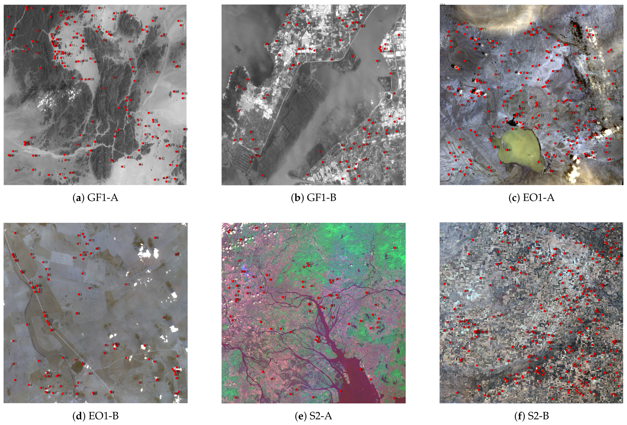
For the first six datasets shown in Figure 1, all GCPs are generated using an automatic image matching approach in which Landsat-8 images are used as geographic reference data. The elevation information of the matching points is derived from the ASTER GDEM V3 dataset. The IKONOS dataset is obtained from an open website, which contains fully independent field-surveyed check points. And it provides the latitude, longitude, elevation and pixel coordinate information for 126 control points. The basic information of the seven datasets is summarized in

Table 2. Basic information of the experimental datasets.

Dataset	Satellite	Scene Type	GSD (m)	Coverage (km2)	Elevation Range (m)	No. of GCPs
GF1-A	GF-1	Mountain	16	$40\times 40$	403–917	200
GF1-B	GF-1	Urban	16	$20\times 20$	−22–280	100
EO1-A	EO-1	Mountain/Lake	30	$30\times 30$	4907–5361	250
EO1-B	EO-1	Rural	30	$27\times 27$	331–437	120
S2-A	Sentinel-2	Urban/River	60	$110\times 110$	−55–1257	80
S2-B	Sentinel-2	Rural	60	$110\times 110$	847–1272	300
IKONOS	IKONOS	Mountain/Urban	1	$120\times 130$	−2–1262	126

, including the satellite platform, scene type, ground sampling distance (GSD), spatial coverage, elevation range, and the number of available GCPs.

GF1-A and GF1-B are GF-1 Wide Field View (WFV) images with a GSD of 16 m. GF1-A corresponds to a mountainous scene with relatively large terrain variations, whereas GF1-B covers an urban area with complex surface structures. EO1-A and EO1-B were acquired by the EO-1 satellite with a GSD of 30 m. EO1-A contains mountainous and lake areas at high elevation, while EO1-B mainly represents a rural scene. S2-A and S2-B are Sentinel-2 images with a GSD of 60 m and a larger spatial coverage. S2-A includes urban and river regions, whereas S2-B is mainly characterized by rural land cover. IKONOS is a high-resolution remote sensing satellite image with a resolution of 1 m, which includes mountainous areas and urban regions. These datasets therefore provide diverse geometric and topographic conditions for evaluating the proposed RPC estimation method. To investigate the influence of both the number and spatial distribution of GCPs, we adopt a random sampling strategy. For each dataset, a fixed number of points is randomly selected from all available matched points and used as GCPs for RPC estimation. The remaining points are not involved in model fitting and are used as independent check points (ICPs) for accuracy assessment.

The image-space root mean square error (RMSE) is used as the primary evaluation metric. Given N ICPs, let ${\epsilon }_{l,i}$ and ${\epsilon }_{s,i}$ denote the residual errors of the i-th ICP in the line and sample directions, respectively. The RMSE is defined as follows:

$$\mathrm{RMSE}=\sqrt{{\displaystyle \frac{1}{N}}\sum _{i=1}^N\left({\epsilon }_{l,i}^2+{\epsilon }_{s,i}^2\right)}.$$

(42)

The RMSE is measured in pixels. A smaller RMSE indicates that the estimated RPCs can more accurately describe the geometric mapping between ground coordinates and image coordinates. To reduce the randomness caused by a single split, each experimental setting is repeated five times. Then, the mean and standard deviation of the RMSE values of the results are reported.

4.2. Parameter Settings

To evaluate the effectiveness of the proposed method, we select four representative RPC estimation methods as competing methods, including Ridge Estimation [10], L1LS [11], LPRFM [12] and ASPCA-RFM [20]. Among them, L1LS introduces an ${\mathsf{\ell }}_1$-norm regularization term into the least-squares framework, which enables stable and sparse RPC estimation when the number of observations is relatively limited. ASPCA-RFM incorporates an Elastic Net sparsity constraint into the principal component analysis procedure, ensuring that each principal component is constructed from only a small subset of the original variables. In this way, redundant or noise-related variables can be automatically removed during principal component computation, leading to a low-rank reconstruction of the design matrix. The parameter settings for all methods are designed to achieve the best experimental results. For Ridge Estimation, the regularization parameter is set to $\lambda ={10}^{-4}$ for consistency with [20]. For L1LS, we follow the optimal setting reported in [11], also setting $\lambda ={10}^{-4}$. And it has been verified that we achieved the best performance under this parameter setting; so, we keep the same parameter setting. For ASPCA-RFM, the parameter configuration was kept consistent with [20] to achieve its best performance. LPRFM is a parameter-free method and therefore requires no additional regularization parameter tuning. The regularization weights of the proposed method are automatically determined according to the scale-normalized strategy described in Section 3.2. The global parameter settings are $c_{\alpha }=50,c_{\lambda }=3\times {10}^{-4},c_{\mu }={10}^{-4},{\kappa }_0=500,{\delta }_l=0.5$. $\tau$ is a dimensionless weighting factor that is used to control the overall strength of the low-rank and PRC parameter sparsity regularization in the potential geometric design matrix. If the value of $\tau$ is too large, it may cause the low-rank and sparse regularization constraints to be too strong, resulting in a deviation between the potential geometric design matrix and the RPC parameters from their true values. On the other hand, if $\tau$ is too small, the low-rank and sparse regularization constraints will be too weak, leading to a decrease in the accuracy of parameter estimation. All experiments were conducted on a computer running Windows 11, equipped with an Intel Core i5-10200H processor and 16 GB of RAM.

4.3. Comparative Experiments

To further evaluate the effectiveness of the proposed method under both underdetermined and overdetermined conditions, comparative experiments are conducted on the six datasets described above. The number of GCPs used for RPC estimation is set to 10, 20, 30, 40, and 50, respectively. Since the RFM contains 78 unknown RPCs and each GCP provides two observation equations, at least 39 GCPs are theoretically required. Therefore, the cases with 10, 20 and 30 GCPs correspond to underdetermined conditions, while those with 40 and 50 GCPs correspond to overdetermined conditions.

For each experimental setting, the selected GCPs are used to estimate the RPCs, and the remaining points are used as independent check points (ICPs) for accuracy assessment. The image-space RMSE calculated on the ICPs is adopted as the evaluation metric. In total, 30 experimental scenarios are constructed from six datasets and five GCP settings. The proposed method is compared with four representative methods, including Ridge Estimation, L1LS, LPRFM and ASPCA-RFM. The experimental results are summarized in

Table 3. The average and standard deviation of RMSE values for different methods on the dataset (in pixels). Bold: the best performance; Underline: the second-best performance.

Dataset	GCPs/ICPs	Ridge Estimation	L1LS	LPRFM	ASPCA-RFM	LRMC-RFM (Ours)
GF1-A	10/190	$286.53\pm 115.45$	$3.83\pm 2.52$	$1.42\pm 0.35$	$\mathbf{1}.\mathbf{17}\pm \mathbf{0}.\mathbf{14}$	$\underline{1.31}\pm \underline{0.20}$
	20/180	$48.84\pm 37.97$	$1.78\pm 0.40$	$\underline{1.00}\pm \underline{0.17}$	$1.12\pm 0.24$	$\mathbf{0}.\mathbf{98}\pm \mathbf{0}.\mathbf{16}$
	30/170	$17.44\pm 16.31$	$1.75\pm 0.65$	$\underline{0.90}\pm \mathbf{0}.\mathbf{09}$	$0.94\pm 0.11$	$\mathbf{0}.\mathbf{87}\pm \underline{0.10}$
	40/160	$4.43\pm 1.63$	$1.59\pm 0.33$	$0.87\pm 0.05$	$\underline{0.85}\pm \underline{0.03}$	$\mathbf{0}.\mathbf{84}\pm \mathbf{0}.\mathbf{03}$
	50/150	$3.00\pm 1.48$	$1.35\pm 0.16$	$\underline{0.86}\pm 0.04$	$0.87\pm \underline{0.04}$	$\mathbf{0}.\mathbf{83}\pm \mathbf{0}.\mathbf{02}$
GF1-B	10/90	$83.93\pm 21.31$	$3.15\pm 4.23$	$\underline{1.59}\pm \mathbf{0}.\mathbf{19}$	$1.80\pm 0.52$	$\mathbf{1}.\mathbf{50}\pm \underline{0.29}$
	20/80	$12.59\pm 5.55$	$1.21\pm 0.27$	$1.13\pm 0.13$	$\underline{1.13}\pm \mathbf{0}.\mathbf{06}$	$\mathbf{1}.\mathbf{03}\pm \underline{0.09}$
	30/70	$16.32\pm 12.78$	$5.68\pm 4.59$	$1.24\pm 0.35$	$\underline{1.01}\pm \underline{0.08}$	$\mathbf{0}.\mathbf{99}\pm \mathbf{0}.\mathbf{05}$
	40/60	$7.88\pm 8.38$	$3.00\pm 3.94$	$\underline{1.00}\pm 0.07$	$1.02\pm \mathbf{0}.\mathbf{05}$	$\mathbf{0}.\mathbf{98}\pm \underline{0.06}$
	50/50	$7.34\pm 10.40$	$3.30\pm 4.28$	$0.99\pm \underline{0.06}$	$\underline{0.98}\pm 0.06$	$\mathbf{0}.\mathbf{96}\pm \mathbf{0}.\mathbf{05}$
EO1-A	10/240	$109.31\pm 33.44$	$1.53\pm 1.09$	$\underline{0.68}\pm \underline{0.09}$	$\mathbf{0}.\mathbf{66}\pm \mathbf{0}.\mathbf{08}$	$0.76\pm 0.17$
	20/230	$24.29\pm 12.45$	$0.80\pm 0.16$	$0.63\pm 0.06$	$\underline{0.61}\pm \underline{0.03}$	$\mathbf{0}.\mathbf{57}\pm \mathbf{0}.\mathbf{03}$
	30/220	$6.37\pm 3.88$	$0.77\pm 0.15$	$\underline{0.53}\pm 0.04$	$0.56\pm \underline{0.02}$	$\mathbf{0}.\mathbf{53}\pm \mathbf{0}.\mathbf{01}$
	40/210	$4.03\pm 1.73$	$0.73\pm 0.09$	$\underline{0.52}\pm \underline{0.02}$	$0.56\pm 0.04$	$\mathbf{0}.\mathbf{52}\pm \mathbf{0}.\mathbf{02}$
	50/200	$1.45\pm 0.59$	$0.68\pm 0.04$	$\underline{0.51}\pm \underline{0.02}$	$0.54\pm 0.04$	$\mathbf{0}.\mathbf{51}\pm \mathbf{0}.\mathbf{01}$
EO1-B	10/110	$145.16\pm 51.85$	$3.65\pm 4.14$	$\underline{1.37}\pm \underline{0.58}$	$\mathbf{1}.\mathbf{05}\pm \mathbf{0}.\mathbf{39}$	$1.49\pm 0.66$
	20/100	$27.49\pm 11.00$	$1.13\pm 0.30$	$\mathbf{0}.\mathbf{74}\pm \mathbf{0}.\mathbf{07}$	$0.83\pm \underline{0.08}$	$\underline{0.83}\pm 0.15$
	30/90	$9.93\pm 5.89$	$0.91\pm \underline{0.10}$	$\underline{0.71}\pm \mathbf{0}.\mathbf{09}$	$0.75\pm 0.12$	$\mathbf{0}.\mathbf{67}\pm 0.10$
	40/80	$4.49\pm 3.55$	$1.00\pm 0.15$	$0.70\pm \underline{0.06}$	$\underline{0.69}\pm \mathbf{0}.\mathbf{06}$	$\mathbf{0}.\mathbf{68}\pm 0.10$
	50/70	$2.20\pm 0.67$	$0.95\pm 0.18$	$\underline{0.68}\pm \underline{0.08}$	$0.69\pm 0.14$	$\mathbf{0}.\mathbf{61}\pm \mathbf{0}.\mathbf{07}$
S2-A	10/70	$168.88\pm 74.62$	$6.00\pm 2.75$	$51.32\pm 72.15$	$\underline{1.20}\pm \underline{0.41}$	$\mathbf{1}.\mathbf{08}\pm \mathbf{0}.\mathbf{15}$
	20/60	$107.85\pm 107.00$	$4.82\pm 3.77$	$7.00\pm 11.05$	$\underline{0.82}\pm \underline{0.24}$	$\mathbf{0}.\mathbf{73}\pm \mathbf{0}.\mathbf{12}$
	30/50	$71.25\pm 95.02$	$3.64\pm 3.43$	$8.85\pm 17.95$	$\mathbf{0}.\mathbf{67}\pm \mathbf{0}.\mathbf{04}$	$\underline{0.78}\pm \underline{0.15}$
	40/40	$36.78\pm 34.18$	$2.04\pm 0.75$	$0.83\pm 0.35$	$\underline{0.65}\pm \underline{0.03}$	$\mathbf{0}.\mathbf{65}\pm \mathbf{0}.\mathbf{03}$
	50/30	$20.59\pm 21.14$	$1.59\pm 0.85$	$0.69\pm 0.11$	$\underline{0.65}\pm \underline{0.04}$	$\mathbf{0}.\mathbf{64}\pm \mathbf{0}.\mathbf{02}$
S2-B	10/290	$107.14\pm 32.42$	$2.16\pm 0.50$	$\underline{1.27}\pm \underline{0.47}$	$1.40\pm 0.54$	$\mathbf{1}.\mathbf{04}\pm \mathbf{0}.\mathbf{15}$
	20/280	$22.72\pm 18.67$	$1.68\pm 0.35$	$0.85\pm 0.17$	$\underline{0.82}\pm \underline{0.07}$	$\mathbf{0}.\mathbf{77}\pm \mathbf{0}.\mathbf{07}$
	30/270	$6.01\pm 3.50$	$1.65\pm 0.30$	$0.78\pm 0.06$	$\underline{0.75}\pm \underline{0.03}$	$\mathbf{0}.\mathbf{72}\pm \mathbf{0}.\mathbf{02}$
	40/260	$2.94\pm 1.51$	$1.71\pm 0.33$	$0.76\pm 0.06$	$\underline{0.74}\pm \mathbf{0}.\mathbf{01}$	$\mathbf{0}.\mathbf{72}\pm \underline{0.03}$
	50/250	$1.93\pm 0.59$	$1.63\pm 0.20$	$\underline{0.73}\pm \mathbf{0}.\mathbf{02}$	$0.73\pm 0.03$	$\mathbf{0}.\mathbf{71}\pm \underline{0.03}$
IKONOS	10/116	$745.92\pm 324.45$	$55.44\pm 39.12$	$\underline{26.55}\pm \underline{30.19}$	$462.94\pm 926.71$	$\mathbf{18}.\mathbf{27}\pm \mathbf{16}.\mathbf{07}$
	20/106	$199.80\pm 206.06$	$31.00\pm 29.09$	$\underline{11.74}\pm \underline{23.58}$	$407.84\pm 846.76$	$\mathbf{8}.\mathbf{22}\pm \mathbf{10}.\mathbf{98}$
	30/96	$51.08\pm 34.21$	$16.94\pm 1.84$	$\underline{3.84}\pm \underline{1.14}$	$36.04\pm 18.42$	$\mathbf{2}.\mathbf{60}\pm \mathbf{0}.\mathbf{85}$
	40/86	$7.98\pm 5.48$	$18.09\pm 4.38$	$\underline{3.28}\pm \underline{0.39}$	$30.49\pm 16.49$	$\mathbf{2}.\mathbf{13}\pm \mathbf{0}.\mathbf{16}$
	50/76	$2.85\pm 0.96$	$14.22\pm 1.51$	$\underline{1.85}\pm \mathbf{0}.\mathbf{06}$	$20.71\pm 2.57$	$\mathbf{1}.\mathbf{78}\pm \underline{0.25}$

. The best result in each row is highlighted in bold and the second-best result is underlined. The mean RMSE directly reflects the positioning accuracy of each method, while the standard deviation indicates its robustness with respect to different GCP spatial distributions.

From the experimental results in Table 3, it can be observed that the proposed method achieves the lowest RMSE in 30 out of 35 scenarios. This indicates that, compared with the competing methods, the proposed method has a higher probability of obtaining more accurate RPC estimates in most cases. For the overdetermined scenarios, where the number of GCPs used for RPC estimation is 40 or 50, the proposed method obtains the lowest RMSE on all datasets. Meanwhile, its standard deviation is also comparable to that of ASPCA-RFM. More importantly, in all overdetermined scenarios, the RMSE values of the proposed method are consistently below 1 pixel, which cannot be achieved by the other competing methods.

In the underdetermined scenarios, where the number of GCPs used for RPC estimation is 10, 20, or 30, RPC estimation is more severely affected by ill-posedness and overfitting. The results show that Ridge Estimation almost fails under such conditions. L1LS and LPRFM can alleviate overfitting to some extent by imposing sparsity constraints on the RPC parameters. For the GF1-B and S2-B datasets, LRMC-RFM achieves the lowest RMSE in all underdetermined cases. Except for the EO1-B dataset, LRMC-RFM generally performs better than ASPCA-RFM on the remaining datasets. It is also worth noting that, in all underdetermined scenarios, the RMSE values of LRMC-RFM remain below 1.5 pixels, which is difficult for the other methods to achieve.

We also compare the average computational time and computational complexity of the proposed method with those of the competing methods, as shown in

Table 4. Average computational time and complexity of different methods.

Ridge Estimation	L1LS	LPRFM	ASPCA-RFM	LRMC-RFM (Ours)
0.0008 s	0.0017 s	0.0068 s	0.0454 s	0.0408 s
$O(n{p}^2+p^3)$	$O\left(T_{L1}np\right)$	$O\left(T_{LP}n(n+p)\right)$	$O(T_{PCA}knp+n{p}^2+p^3)$	$O\left(T_{ADMM}[npmin(n,p)+n{p}^2+p^3]\right)$

. $n=2m$, $p=78$, k is the number of retained principal components, and $T_{L1}$, $T_{LP}$, $T_{PCA}$, and $T_{ADMM}$ denote the corresponding iteration numbers. Since LRMC-RFM requires iterative optimization based on ADMM, its average computational time is longer than those of Ridge Estimation, L1LS, and LPRFM. However, it is slightly shorter than that of ASPCA-RFM. This demonstrates that the proposed method maintains high estimation accuracy while keeping the computational cost at a moderate level. Moreover, the average runtime of all methods remains sufficiently low for real-time implementation.

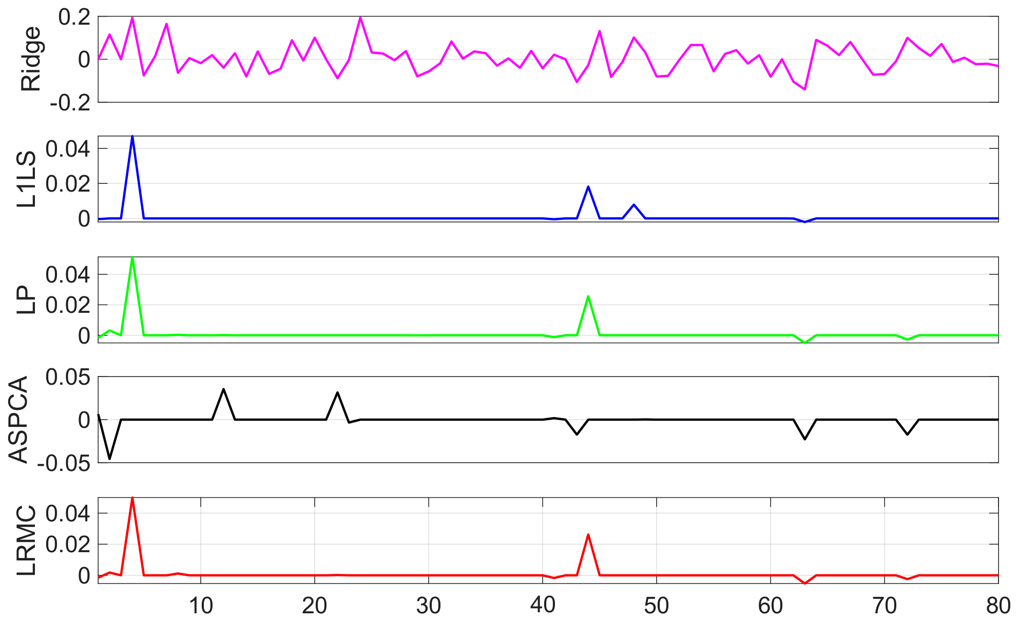
We plot the RPC parameters estimated by all methods when the number of GPCs is 10 on the IKONOS dataset, and the results are shown in Figure 2. In order to better observe the sparsity of the estimated RPC parameters, we set the components whose norm is close to 1 to zero. It can be observed that the RPC parameters estimated by our method have similar sparsity with the PRC parameters estimated by LPRFM method, and are more obvious than other methods.

4.4. Model Analysis

4.4.1. Sensitivity Analysis

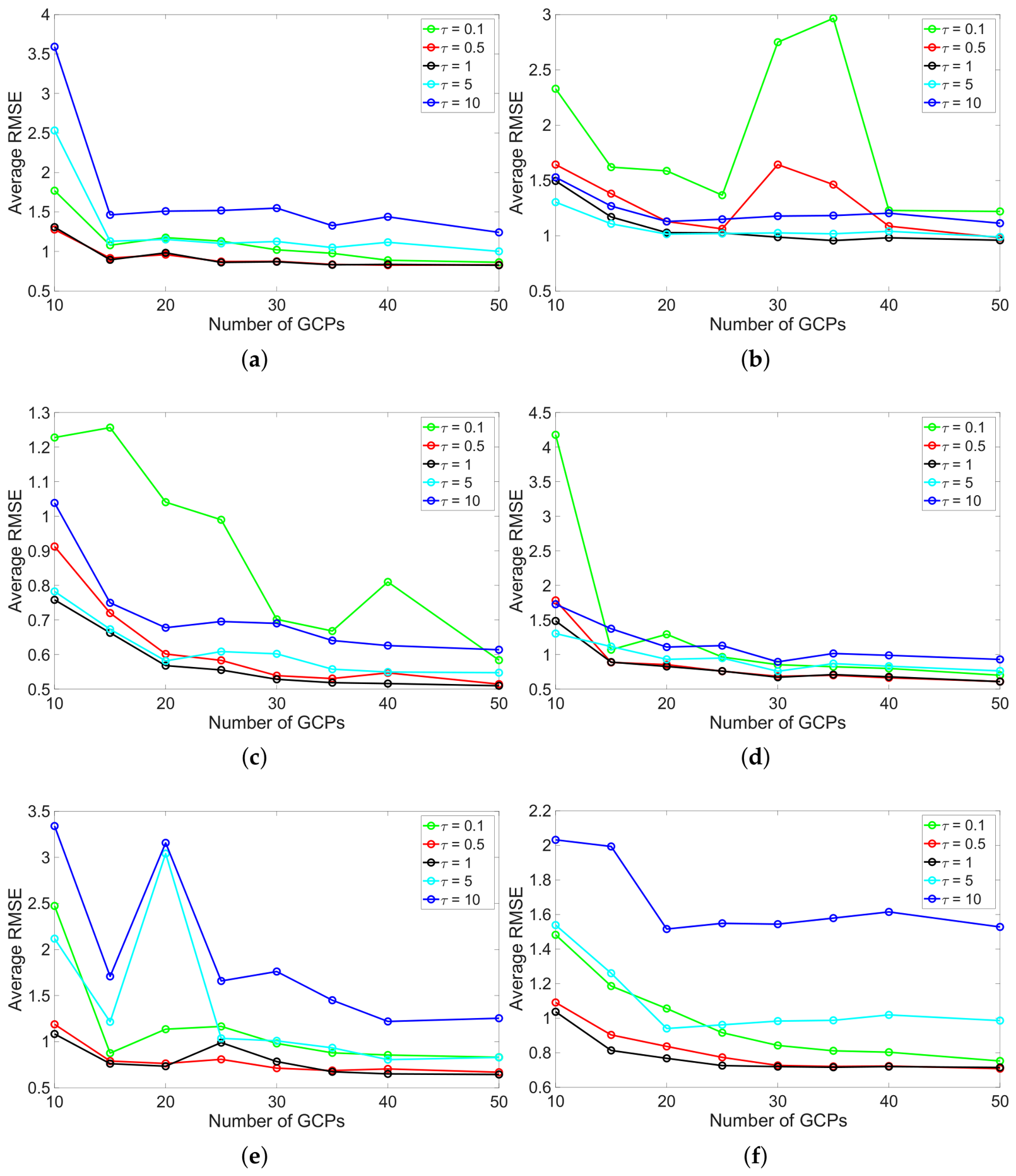
To analyze the influence of the unified regularization strength on the performance of the proposed method, we further test $\tau \in \{0.1,0.5,1,5,10\}$. For each value of $\tau$, the average RMSE is computed on the six experimental datasets under different numbers of GCPs. This experiment aims to evaluate the sensitivity of the proposed scale-normalized regularization strategy to $\tau$, and to verify the rationality of using $\tau =1$ as the default setting. The corresponding results are shown in Figure 3.

The experimental results show that different values of $\tau$ have a noticeable impact on the positioning accuracy. When $\tau =0.1$, the regularization strength is relatively weak, and the low-rank constraint on the design matrix and the sparsity constraint on the RPC parameters are insufficient. As a result, relatively large RMSE values appear on several datasets, especially under sparse GCP conditions. This indicates that under-regularization cannot effectively suppress the instability caused by the ill-posed design matrix and redundant RPC parameters. In contrast, when $\tau =5$ or $\tau =10$, the average RMSE increases on most datasets, suggesting that overly strong regularization may reduce the ability of the model to represent the true geometric mapping and thus lead to underfitting.

By comparison, $\tau =0.5$ and $\tau =1$ exhibit better stability across the six datasets. Among them, $\tau =1$ achieves the lowest or near-lowest average RMSE under most GCP settings, resulting in the best overall performance. This demonstrates that a moderate regularization strength can achieve a better balance among data fitting, low-rank design matrix recovery, and RPC parameter sparsity. Based on the results obtained from all six datasets, $\tau =1$ is adopted as the default unified regularization strength in this study and is kept unchanged in all experiments, without dataset-specific parameter tuning. These results further demonstrate that the proposed scale-normalized regularization strategy has good cross-dataset adaptability and parameter robustness.

4.4.2. Ablation Experiments

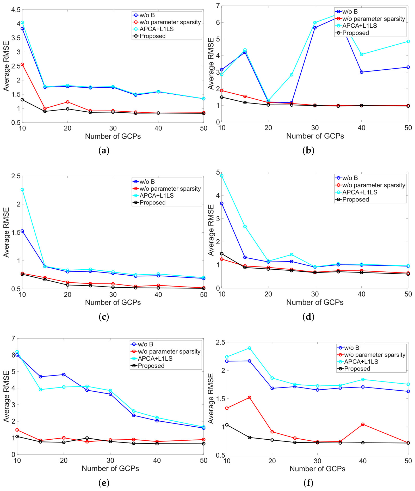
To further verify the necessity of each component in the proposed objective function, we conduct three ablation experiments based on the complete LRMC-RFM method. The corresponding results are shown in Figure 4.

The first ablation variant is denoted as w/o B. In this variant, the low-rank design matrix recovery process is removed and $B=A$ is directly imposed. That is, the original observed design matrix is used for parameter estimation without low-rank correction. Under this setting, the model degenerates into a sparse RPC parameter estimation problem with only the ${\mathsf{\ell }}_1$-norm regularization term.The second ablation variant is denoted as w/o parameter sparsity. In this variant, the sparsity constraint on the RPC parameter vector is removed. Therefore, the RPC parameters are no longer selected by the ${\mathsf{\ell }}_1$-norm regularization. Instead, the design matrix is processed through a PCA-type dimensionality reduction or low-rank reconstruction procedure, and the RPC parameters are then estimated based on the reconstructed matrix. The third ablation variant is denoted as APCA+L1LS. In this ablation method, the design matrix is first reconstructed by the APCA [19] algorithm without parameters, and then the reconstructed design matrix and the observed values are solved by L1LS. The parameter settings of the used method are all consistent with those in Section 4.2, including APCA + L1LS.

By looking at the experimental results in Figure 4, we found that removing the low-rank matrix variable B leads to a significant increase in root mean square error (RMSE), especially on the GF1-B and S2-A datasets. Under sparse GCP conditions, the results become highly unstable, indicating that directly using the original ill-posed design matrix may amplify observation noise and reduce the extrapolation stability of RPC estimation. Compared with the variant without sparse RPC regularization, the complete LRMC-RFM generally achieves lower RMSE in most experimental settings. This indicates that the sparsity constraint on RPC parameters further alleviates the over-parameterization problem of the complete third-order RFM. Although the model without sparse regularization can still obtain relatively competitive performance in a few cases, the complete model achieves the best overall accuracy and stability across all datasets. In addition, the two-stage method shows the worst performance among the compared variants, further demonstrating that the advantages of low-rank design matrix recovery and sparse RPC estimation cannot be effectively exploited by a simple sequential combination. Such a decoupled strategy may even deteriorate the parameter estimation accuracy, which can be attributed to error accumulation between the two stages and potential over-regularization caused by imposing successive constraints. The ablation results show that both the recovery of the low-rank design matrix and the sparse RPC regularization contribute to the final accuracy of the proposed method. The proposed unified optimization framework can more effectively integrate the advantages of low-rank design matrix recovery and sparse RPC estimation, rather than merely combining them in a sequential or additive manner.

4.4.3. Initialization Analysis

Since there is a quadratic coupling between B and $\theta$ in the objective function proposed in this paper, the overall objective function is non-convex. The initialization of parameters may affect the final solution process. For initialization, PCA-RFM is first used to obtain an initial estimate of the RPC parameters. If the PCA-based initialization fails, a lightly regularized Ridge estimate is adopted as a fallback, which improves numerical stability under extremely sparse GCP conditions. The initial value $B^0$ of parameter B is obtained by performing low-rank reconstruction on the design matrix A based on principal component analysis. The split variables and scaled dual variables are initialized by $Z^0=B^0$, ${\xi }^0={\theta }^0$, $U^0=0$, $u^0=0$.

To investigate the practical dependence of the proposed ADMM-based solver on the initial values, we conduct two ablation experiments on GF1-A dataset. The first ablation variant is an initialization strategy designed for the low-rank matrix B. In the first strategy, the design-matrix variable is directly initialized using the observed matrix, i.e., $B^0=A$. The initialization method of RPC parameters $\theta$ is consistent with that of LRMC-RFM. The second ablation variant is an initialization strategy designed for the RPC parameters $\theta$. In the second strategy, the initial RPC parameters ${\theta }^0$ is obtained by Ridge estimation. The initialization method of B is consistent with that of LRMC-RFM.All other regularization parameters, ADMM penalty parameters, stopping criteria, and experimental settings are kept identical. The results are shown in

Table 5. Average and standard deviation values (in pixels) for different initialization methods evaluated on GF1-A dataset. Bold: the best performance; Underline: the second-best performance.

Dataset	GCPs/ICPs	${\mathit{B}}^0$	${\mathit{\theta }}^0$	LRMC-RFM (Ours)
GF1-A	10/190	$\mathbf{1}.\mathbf{30}\pm \underline{0.20}$	$1.32\pm 0.21$	$\underline{1.31}\pm \mathbf{0}.\mathbf{20}$
	20/180	$0.98\pm 0.16$	$1.78\pm 0.16$	$\mathbf{0}.\mathbf{98}\pm \mathbf{0}.\mathbf{16}$
	30/170	$0.87\pm 0.10$	$0.87\pm 0.10$	$\mathbf{0}.\mathbf{87}\pm \mathbf{0}.\mathbf{10}$
	40/160	$0.84\pm 0.03$	$0.84\pm 0.03$	$\mathbf{0}.\mathbf{84}\pm \mathbf{0}.\mathbf{03}$
	50/150	$0.83\pm 0.02$	$0.83\pm 0.02$	$\mathbf{0}.\mathbf{83}\pm \mathbf{0}.\mathbf{02}$

. The results indicate that, in most tested configurations, the proposed ADMM-based optimization procedure exhibits low empirical sensitivity to the initialization and converges to solutions with nearly identical generalization accuracy.

5. Conclusions

This paper proposes a sparse RPC estimation method via the low-rank matrix constraint. By jointly estimating the low-rank design matrix B and the sparse RPC parameter vector $\theta$ under a unified optimization framework, the ill-posed and over-parameterized problems in RPC parameter estimation are effectively alleviated. In addition, an efficient ADMM-based optimization solver is derived. In this solver, singular value soft thresholding is used to enforce the low-rank constraint, element-wise soft thresholding is used to enforce sparsity, and closed-form expressions are used to obtain the update of the design matrix. The experimental results show that the proposed method achieves the best RMSE performance in 25 out of 30 scenarios across 6 datasets. Ablation experiments further confirm the effectiveness of joint low-rank design matrix recovery and sparse RPC parameter estimation.