Article

An Integrated Deep Learning Approach to Estimate Canopy Height and Uncertainty by Combining Seasonal Optical, SAR and Limited GEDI LiDAR Data over Ontario’s Managed Forests, Canada


1
School of Earth, Environment & Society, McMaster University, 1280 Main Street West, Hamilton, ON L8S 4K1, Canada
2
Department of Geography and Environmental Studies, Toronto Metropolitan University, 350 Victoria Street, Toronto, ON M5B 2K3, Canada
3
Planet Labs PBC, San Francisco, CA 94107, USA
4
Environment and Climate Change Canada, Gatineau, QC K1A 0H3, Canada
*
Author to whom correspondence should be addressed.
Remote Sens. 2026, 18(15), 2477; https://doi.org/10.3390/rs18152477
Submission received: 25 May 2026 / Revised: 6 July 2026 / Accepted: 16 July 2026 / Published: 29 July 2026
(This article belongs to the Section Forest Remote Sensing)

Highlights

What are the main findings?
  • The Laplace-loss ResUNet ensemble reduced canopy-height bias and achieved 3.65 m RMSE against independent airborne LiDAR.
  • Seasonal optical and SAR inputs improved canopy-height accuracy, while SAR-only models outperformed the tested global products across forest classes.
What are the implications of the main findings?
  • More accurate, less biased canopy-height estimates can improve aboveground biomass and forest carbon-stock mapping.
  • SAR-based canopy-height mapping can support biomass applications in cloud-prone northern forests where optical observations and LiDAR samples are limited.

Abstract

Accurate canopy-height mapping is essential for forest carbon monitoring, yet spatially continuous estimates over northern forests remain limited by sparse LiDAR sampling and unreliable optical data. We present a probabilistic deep learning framework that integrates seasonal Landsat optical, Sentinel-1 C-band SAR, and yearly ALOS-PALSAR-2 L-band SAR composites with GEDI training targets to produce 30 m canopy-height and pixel-level uncertainty maps over Ontario, Canada. A ResUNet ensemble is trained with a Laplace negative log-likelihood (NLL) loss; aleatoric and epistemic uncertainty are captured through a mixture of Laplace distributions, calibrated post hoc by Platt scaling and validated against airborne LiDAR (ALS P98). Under matched architecture and inputs, replacing Gaussian with Laplace NLL improved R 2 by 18.6%, reduced RMSE by 13.7%, and cut systematic bias from 1.43 to 0.14 m. The primary model reached R 2 = 0.70 , RMSE = 3.65 m, and bias = 0.23 m, exceeding GEDI’s own footprint-level agreement with the independent ALS reference within Ontario’s managed forest zone. Seasonal compositing raised R 2 by 12.9% over summer-only inputs, and SAR-only configurations outperformed four global products in every forest class. The framework also delivers a calibrated, pixel-level uncertainty layer that reflects local structural difficulty beyond canopy height and can serve as a confidence layer for downstream carbon-stock and forest-management applications.

1. Introduction

Accurate estimates of forest aboveground biomass (AGB) are essential to assess forest carbon stocks and their change over time to support policies to reduce climate change, manage resources, and preserve biodiversity [1,2,3,4,5]. Canopy height (CH), a variable that can be directly obtained from remote sensing observations, is used as a predictor of AGB in many studies due to its close relationship to tree biomass [1,6,7,8,9,10,11]. In addition, canopy height is also critical to accurately estimate carbon sequestration rates, since the rate of carbon assimilation into biomass increases continuously with the size of trees [12].
Airborne Light Detection and Ranging (LiDAR) is the preferred means to provide highly accurate and precise measurements of canopy height and, unlike field observations, allows for height measurements to be taken from remote and for larger areas in a timely manner. However, airborne LiDAR (ALS) campaigns have limited spatial coverage and tend to be expensive, leading most acquisitions to focus on areas of high value forests [13,14]. To address this limitation, the Global Ecosystem Dynamics Investigation (GEDI) spaceborne LiDAR sensor onboard the International Space Station (ISS) provides near-global sampling of canopy structure. The GEDI mission uses a laser altimeter to measure the distance from the ISS to the Earth’s surface with high accuracy and spatial resolution [15]. GEDI does not provide a spatially continuous canopy-height map. Instead, it captures 25 m spatial resolution footprint samples on the Earth’s surface following a sparse grid-based sampling pattern between 51.6°N and 51.6°S. GEDI samples are spaced every 60 m in the along-track direction and 600 m in the across-track direction [16]. The contrast between the sparse, footprint-based sampling of spaceborne GEDI and the continuous but spatially limited wall-to-wall coverage of airborne LiDAR is illustrated in Figure 1.
To extrapolate GEDI LiDAR measurements and build wall-to-wall canopy height maps, many studies make use of other sensor data and machine learning methods. For example, Qi et al. [9,17] used GEDI to improve height estimates provided by TanDEM-X Interferometric Synthetic Aperture Radar (InSAR), initially focusing on sites in the United States and Costa Rica, with subsequent extensions to Mexico, the Amazon Basin, French Guinea, and Gabon. However, their approach involved InSAR processing, which is computationally intensive and not readily scalable, particularly given the lack of TanDEM-X data availability on platforms like Google Earth Engine (GEE), and TanDEM-X data is not freely accessible [18]. Silveira et al. [19] produced 30 m resolution maps of forest structure across Argentina by training random forest models on national forest inventory plots, incorporating spatially explicit uncertainty estimates. At a national scale, Sothe et al. [20] tested both Ice, Cloud, and land Elevation Satellite-2 (ICESat-2) and GEDI LiDAR observations together with Sentinel-1 and -2, ALOS-PALSAR-2 data, and a random forest model to map forest canopy height in Canada at a 250 m spatial resolution with RMSE of 4.2 m. At a global scale, Potapov et al. [21] used GEDI canopy height data with Landsat data and a tree ensemble model to produce a 30 m spatial resolution forest canopy-height map with RMSE of 9.1 m. More recently, Travers-Smith et al. [22] used satellite LiDAR from ICESat-2, Landsat data, and a random forest model to map canopy height of northern forest-tundra areas in Canada. A common limitation with tree-ensemble methods like random forests is that predictions are resulting from the average values of many decision trees, which undermines their ability to predict canopy height for very short or tall canopy-height values [22,23]; tree-ensemble methods also exhibit high sensitivity to input data quality, poor performance with small training sets, and failure to extrapolate beyond the training range [24].
Recent work indicates that deep learning (DL) methods can outperform tree-ensemble methods for canopy-height mapping because they learn hierarchical feature representations directly from high-dimensional inputs and can exploit spatial context, and because their network architecture and loss function can be tailored to noisy, extreme-valued targets [25]. Lang et al. [26] first demonstrated this paradigm at global scale, training an ensemble of CNNs with a Gaussian negative log-likelihood (NLL) loss on Sentinel-2 imagery and GEDI labels to produce 10 m canopy height with pixel-level uncertainty. Lang et al. [27] refined this approach with a weighted loss and updated training set, retaining the Gaussian NLL formulation and ensemble-based uncertainty. Pauls et al. [28] extended global mapping further by introducing a shift-tolerant loss that mitigates GEDI’s geolocation error in Sentinel-1/2 composites, and Fayad et al. [25] explored a vision transformer with a discrete/continuous weighted loss in Ghana to improve sensitivity to tall trees, though that latter study did not provide pixel-level uncertainty or seasonal compositing. Other DL-based regional efforts include Liu et al. [29], who used a U-Net with 3 m Planet imagery to map canopy height across Europe (RMSE = 5.4 m); Tolan et al. [30], who applied a self-supervised DINOv2 model to 0.59 m Maxar imagery for California and São Paulo; and Wagner et al. [31], who achieved submetre canopy height for California with a regression U-Net trained on 0.6 m USDA-NAIP imagery. While the high-resolution studies improve spatial detail, they depend on commercial imagery and high-end GPUs that are not broadly available, limiting transferability to data-scarce regions.
Across these studies, several gaps remain unresolved. First, current global DL canopy-height models either rely on optical-only inputs [21,26,27] or combine optical with a single SAR frequency [25,28]; to our knowledge, no published deep learning model couples multi-frequency SAR (C-band and L-band) with seasonal optical composites within a single regression framework. This is a relevant gap because optical reflectance, despite its known correlation with canopy structure [32,33,34], saturates above approximately 40–50 m or 150–200 Mg/ha of biomass [21,30,31,35], and is unavailable in persistently cloudy regions. SAR backscatter, in contrast, penetrates the canopy with depth that scales with wavelength [36], so combining C- and L-band with phenological optical context targets exactly the regime where each sensor alone is least informative. Second, the only published probabilistic CNN frameworks for canopy height [26,27] adopt the Gaussian NLL loss, which is poorly suited to the heavy-tailed noise structure of GEDI training labels. Third, the contribution of seasonal data to performance has not been disentangled from sensor contributions across forest types, limiting operational guidance about which inputs matter most where.
A regionally focused study by Sothe et al. [20], which used GEDI as a reference and combined optical with SAR predictors in a random forest model across Canada, reported systematic underestimation of canopy height attributed to limited GEDI training samples and the well-documented inability of tree-ensemble models to extrapolate beyond their training range [23,24]. In that work, Ontario—Canada’s second-largest province, with 70.5 Mha of forest spanning temperate, boreal, and tundra ecosystems and a deep ALS archive—supplied most of the GEDI training data. The combination of substantial within-province ecological gradients, a sparse but consistent GEDI sampling pattern south of 51.6°N, and the ALS archive makes Ontario an exacting testbed for evaluating whether a DL framework that explicitly models prediction uncertainty can resolve the underestimation reported by tree-based regional models.
Pixel-level uncertainty is also unevenly addressed across published canopy-height products. Most regional and national maps report only aggregate accuracy metrics [20,28,31,37], and although Lang et al. [26,27] pioneered ensemble-based pixel-level uncertainty for global canopy-height mapping, the calibration of those estimates against external data, and their behaviour across forest types and structural transitions, has received limited scrutiny. Reliable uncertainty maps are nevertheless essential for downstream use: they identify regions where predictions should not be trusted in carbon-stock accounting or forest planning, and they support adaptive sampling strategies for ground or airborne campaigns [37].
Building on these gaps, we present a Convolutional Neural Network with Uncertainty estimates (UCNN) that produces 30 m canopy-height and pixel-level uncertainty maps over Ontario, Canada, for 2019–2020. The model is a ResUNet-based fully convolutional network trained with a Laplace NLL loss, deployed as an ensemble whose mixture-of-Laplace output captures aleatoric and epistemic uncertainty, with post hoc Platt-scaling calibration. To limit spatial autocorrelation, we partition the study area into 100 non-overlapping tiles and apply five-fold spatial validation within the portion supported by GEDI and the independent ALS reference. The study makes four contributions. First, we introduce a multi-sensor framework that integrates seasonal optical (Landsat) and C-band SAR (Sentinel-1) composites with yearly L-band SAR (ALOS-PALSAR-2) and quantify, by ablation, how each component contributes to predictive performance and to the mitigation of signal saturation in tall canopies. Second, we replace the Gaussian NLL of prior probabilistic CNN canopy-height frameworks with a Laplace NLL and isolate its effect under matched architecture and inputs. Third, we show that, within the Ontario test domain, SAR-only configurations outperform four evaluated global canopy-height products across every forest type, an operationally relevant result for cloud-prone regions. Fourth, we report calibrated, ensemble-based pixel-level uncertainty maps and demonstrate that the calibrated uncertainty reflects local structural heterogeneity independent of canopy magnitude, supporting their use as a confidence layer for downstream applications.

2. Materials and Methods

2.1. Study Area

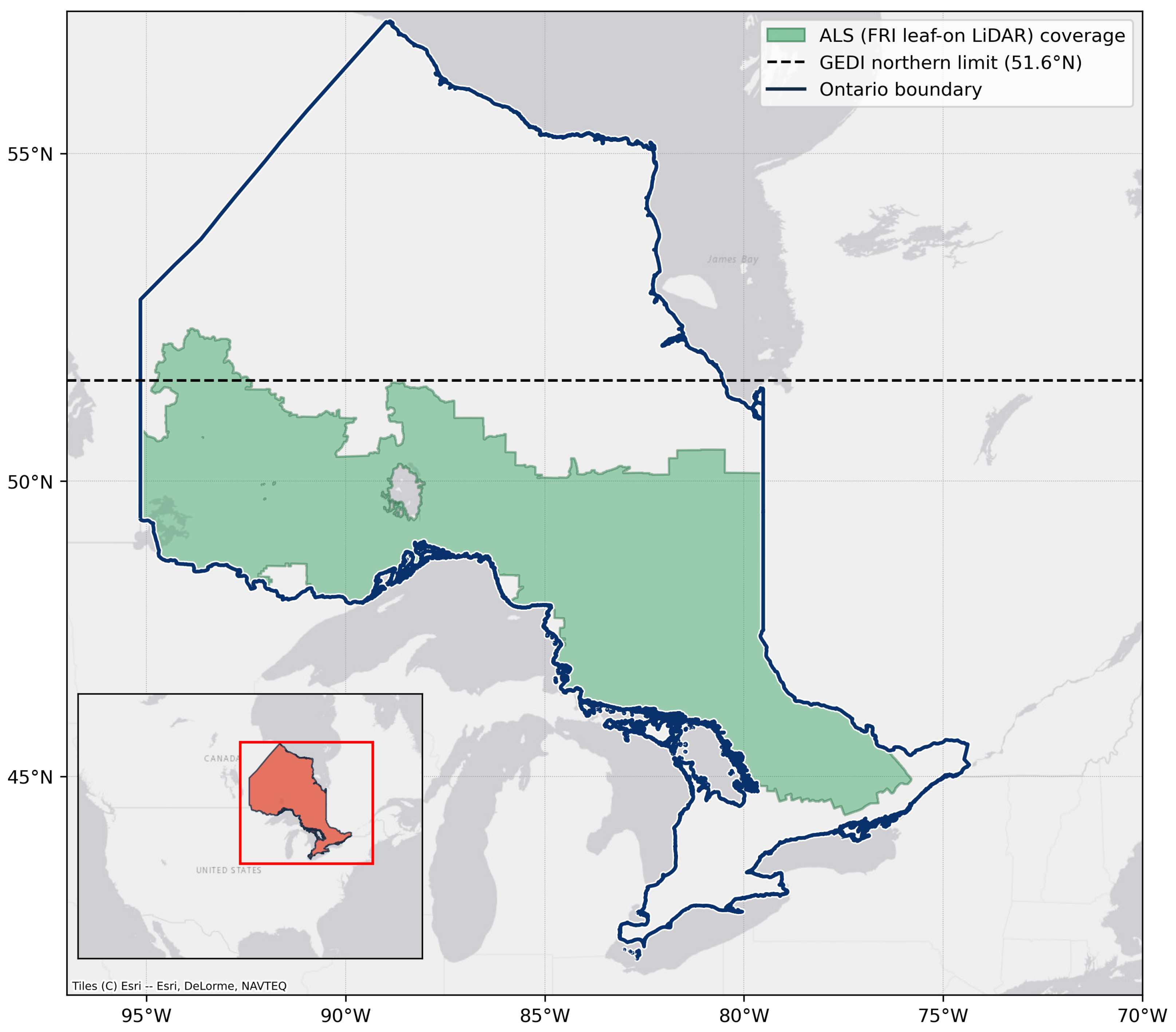
Experiments were conducted between 2019 and 2020 in Ontario, Canada, the second largest province in the country, encompassing 1.076 million km2 (Figure 2). GEDI observations extend to approximately 51.6°N, and the FRI ALS program provides a dense, wall-to-wall canopy-height reference across Ontario’s managed forest zone; the extents of both are shown in Figure 2. Tiles beyond GEDI coverage are used for wall-to-wall inference, and model validation is performed at the locations where GEDI-supported predictions intersect the independent ALS footprint. Ontario’s climate is continental, characterised by humid conditions in the south with cold winters and warm summers, transitioning to a sub-arctic regime in the north. The province’s forests are classified into four primary regions: the Hudson Bay Lowlands in the far north with tundra forest, the boreal forest region and the Great Lakes–St. Lawrence Forest in the south and central areas, and deciduous forest in the south, the latter two encompassing temperate and boreal forests. The Hudson Bay Lowland is dominated by stunted Tamarack and Black Spruce on well-drained areas with occasional presence of White Birch, Dwarf Birch, and Willow. Ontario is part of the Boreal Shield Ecozone, which contains conifer species such as Black and White Spruce, Jack Pine, Balsam Fir, Tamarack, and eastern White Cedar, and a few deciduous species such as Poplar and White Birch. The Great Lakes–St. Lawrence Forest is dominated by deciduous species such as Maple, Oak, Yellow Birch, White and Red Pine, and mixed forests containing White Pine, Red Pine, Hemlock, White Cedar, Yellow Birch, Sugar and Red Maples, Basswood, and Red Oak. The deciduous forest is the southernmost region in Ontario, dominated by agriculture and urban areas, with scattered woodlots containing mainly southern deciduous trees and trees that are found in the Great Lakes–St. Lawrence forests. The spatial distribution of the four forest classes used for the stratified analysis (coniferous, deciduous, mixedwood, and treed-wetland) is derived from the 2020 North American Land Cover map (NALCMS, 30 m) [38] and shown in Figure S1a (Supplementary Materials).

2.2. Data

2.2.1. Satellite Data and Pre-Processing

In this study, we used spaceborne observations from Landsat 7 and 8, Sentinel-1, ALOS-PALSAR-2, and GEDI sensors, all acquired and pre-processed on the Google Earth Engine (GEE) platform [39]. Sentinel-1 and ALOS-PALSAR-2 operate in the C and L bands, respectively, capturing complementary structural details of the trees, with the first interacting primarily with the leaves and the top of the canopy and the latter with the branches and trunks. Landsat sensors add spectral information that characterises vegetation structure and phenology through the reflectance of the forest. A visual comparison of the multi-sensor inputs and the ALS height reference over representative regions is provided in Figure S2 (Supplementary Materials).
The datasets were projected to a common EASE-Grid 2.0 North projection with WGS84 datum at 30 m spatial resolution to match the native Landsat pixel size. The study period spans 2019–2020, aligned with the temporal overlap of ALOS-PALSAR-2 and GEDI. For each year, we constructed seasonal three-month median composites from Landsat and Sentinel-1 over three windows: winter (January–March), summer (June–August), and fall (September–November). The spring shoulder months (April and May) and December were excluded because, across Ontario’s strong south–north climatic gradient, these months span a transition period in which snow cover varies sharply between years and sub-regions, producing seasonal composites that are not stable across the study domain. The retained windows capture, respectively, the snow-on/leaf-off state, peak greenness, and the post-senescence leaf-off state, which together encode the bulk of the canopy’s phenological cycle that is informative for structure retrieval. ALOS-PALSAR-2 is supplied as an annual composite—specifically, the JAXA Global PALSAR-2/PALSAR Yearly Mosaic available on Google Earth Engine—because its temporal sampling is too sparse to support reliable three-month medians at this latitude. A detailed summary of the covariates supplied to the model is presented in Table 1.
To address outliers, noisy data, and gaps in the median seasonal composites for Landsat and Sentinel-1 observations, we introduce the Seasonal Image Composite Algorithm (SICA), as detailed in Algorithm 1, developed on the GEE platform. Inspired by the Multi-year Best Available Pixel (BAP) [40] algorithm, SICA facilitates the generation of smooth image composites for both optical and SAR data by calculating the median value of all valid observations at each pixel location over the analyzed period. In cases where a pixel lacks enough valid observations for a given year and season, SICA employs a recursive approach to retrieve data from the same season in previous years at the same pixel location. We configured SICA with N = 3 maximum recursive iterations and w = 3 years temporal window for retrieving fallback observations from previous years. This strategy mitigates the impact of data acquisition gaps on computed statistics, ensuring the robustness of the generated image composites. The algorithm is also easily adaptable to various types of sensors, depending on the criteria defined for valid observations.
Algorithm 1 Seasonal Image Composite Algorithm (SICA)
Require: Y: Year; S N : Season; S R : Sensor; R O I : Region of Interest; N: minimum number
  of observations at each pixel location; W: number of years back considered.
   I t a r g e t C o l l e c t i o n ( 0 ) m × n                 ▹ initialise the target collection with an empty image collection
  while  ω W   do
     I c o u n t e r pixel _ counter ( I t a r g e t C o l l e c t i o n )                                                     ▹ count valid observations per pixel
     I C o l l e c t i o n get _ image _ collection ( Y , S N , S R , R O I )                   ▹ gather images matching Y, S N ,
S R , R O I
    if  S R is optical then
         I C o l l e c t i o n masking _ pixels ( I C o l l e c t i o n , S N )                ▹ mask out clouds, shadows, snow,
etc.
    end if
     I t a r g e t C o l l e c t i o n ( w ) concat _ collections( ( [ I t a r g e t C o l l e c t i o n , I C o l l e c t i o n ] , I c o u n t e r )                                       ▹ concatenate
only at pixels with fewer than N valid observations
     Y Y 1                                                                                                                                                                                                   ▹ update the target year
end while
I c o m p med ( I t a r g e t C o l l e c t i o n ( w ) )                                                                                                                                 ▹ compute the median image
return  I c o m p
For Sentinel-1, we used the Sentinel-1 SAR Ground Range Detected (GRD) dataset on GEE. We retained images acquired with VV (vertical–vertical) and VH (vertical–horizontal) polarisations, interferometric wide (IW) acquisition mode, and the ascending orbital pass; descending orbits were excluded because of missing acquisitions during 2019–2020. Terrain correction was applied through the GEE implementation of the Range-Doppler Terrain Correction algorithm. For Landsat 7 and 8, we used Tier 1 surface-reflectance products from Collection 2 to maximise per-season observation density and improve the chance of obtaining cloud-free pixels. Pixels flagged as Dilated Cloud, Cirrus, Cloud, or Cloud Shadow in the QA_PIXEL bit mask were removed before seasonal median compositing; snow-flagged pixels were additionally removed from the summer and fall composites. The winter (January–March) composite retains snow-covered pixels, as snow cover is near-ubiquitous across Ontario’s managed forest zone in this window. The composite therefore captures a stable snow-on/leaf-off state, in which the high-albedo snow background against the darker, protruding canopy provides an informative structural cue, and the corresponding C-band Sentinel-1 backscatter captures the frozen-canopy/dry-snow regime. Wet-snow and partial-melt conditions can perturb both optical albedo and C-band backscatter and may add noise in the 0–5 m range where the snow-to-canopy contrast is weakest, an effect examined in Section 4.7. Because the available bands differ between Landsat 7 and 8, we kept only the bands common to both sensors—blue, green, red, near-infrared (NIR), and shortwave infrared 1 (SWIR1)—and renamed them to a unified naming convention before merging into a single Landsat image collection on which the recursive compositing scheme was applied. For ALOS-PALSAR-2, we used the JAXA-provided Global PALSAR-2/PALSAR Yearly Mosaic for the corresponding year, retaining the HH and HV polarisations; because the JAXA mosaic is itself a temporally aggregated product, no additional compositing was performed.
From GEDI, we used the L2A relative height 98th percentile (RH98) metric, restricted to the summer months (June–August) to coincide with full leaf-on conditions, during which RH98 most consistently reflects vertical canopy structure rather than mid-season phenological transitions. RH98 has shown high alignment with airborne LiDAR reference products in prior work [16,20,37]. We discarded coverage beams and retained only full-power beams, kept shots whose L2A binary quality flag indicated valid measurements, and excluded shots flagged for degraded geolocation. Shots with RH98 values outside the plausible physical range for the study area—either negative, or exceeding 40 m—were also removed. The 40 m upper threshold was set with reference to the FRI ALS archive, in which canopy heights above 40 m are extremely uncommon in Ontario’s managed forest zone, consistent with documented stand-level maxima for Ontario boreal and Great Lakes–St. Lawrence forests [41] and with GEDI’s well-documented tendency to return anomalously high RH98 values over steep terrain or with sparse waveform energy. Filtering at 40 m therefore removes implausible outliers while retaining essentially all true canopy variation observed in the regional ALS reference data.

2.2.2. Reference Airborne LiDAR (ALS) Data

To validate the accuracy of both GEDI data and our model estimates, we used the leaf-on Single Photon LiDAR (SPL) product acquired from the Forest Resources Inventory (FRI), Ontario Ministry of Natural Resources and Forestry, available through the Ontario GeoHub data archive [42]. The SPL data were acquired under leaf-on conditions to ensure that the full canopy structure is captured, with a minimum point density of 25 points/m2. The FRI provides three raster products: a Digital Terrain Model (DTM), a Digital Surface Model (DSM), and a canopy-height model (CHM), where CHM = DSM − DTM. For our experiments, we used the CHM raster products spanning 2019–2020. The CHM data are structured into non-overlapping tiles, each with 1000 × 1000 pixels at 0.5 m spatial resolution, totalling approximately 28,000 tiles per year. The SPL acquisition covers approximately 555,000 km2 of Ontario’s managed forest zone, which does not extend to the full provincial area—particularly the remote Hudson Bay Lowlands and Far North regions (Figure 2 and Figure S1).

2.2.3. Global Canopy-Height Products

We benchmarked our model and GEDI against four publicly available global canopy-height products: Meta [30], Lang et al. [27], Potapov et al. [21], and Pauls et al. [28]. The four products differ substantially in input data, target variable, native spatial resolution, and training period, which complicates direct quantitative comparison; we therefore summarise their key attributes in Table 2 and interpret comparison results in light of these differences.
Meta is the highest-resolution product (1 m), generated by a self-supervised DINOv2 vision transformer [43] trained largely on commercial high-resolution imagery acquired in 2018–2020; the authors report an MAE of 2.8 m for selected reference areas. The product of Potapov et al. [21] is a 30 m product for 2019, produced by a bagged regression-tree ensemble linking GEDI RH95 to multi-temporal Landsat-8 surface-reflectance indices, with a reported RMSE of 9.07 m and MAE of 6.36 m against airborne LiDAR. The product of Lang et al. [27] is a 10 m probabilistic deep learning product trained to predict GEDI canopy heights from Sentinel-2 imagery with a weighted loss to handle the heavy-tailed height distribution, achieving a reported RMSE of 7.9 m. The product of Pauls et al. [28] is a global model that incorporates a shift-tolerant loss to mitigate GEDI geolocation noise on Sentinel-1/2 composites and uses SRTM data to filter samples in complex terrain, achieving an MAE of 2.43 m and an RMSE of 4.73 m globally.

2.2.4. Spatial Co-Location and Statistical Aggregation of GEDI with Reference Datasets

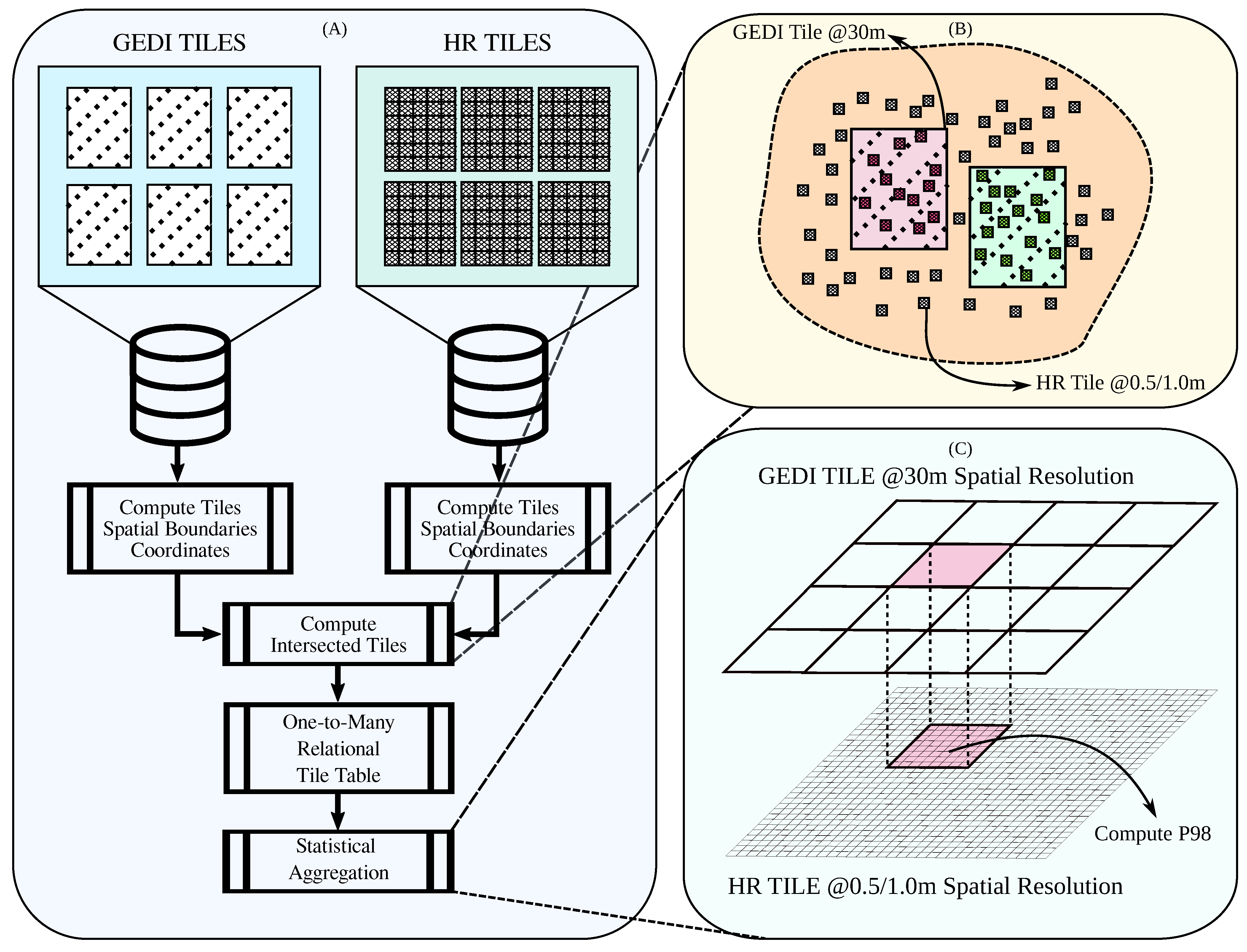
The validation reference for all comparisons in this paper is the airborne LiDAR (ALS) archive. To bring GEDI and the submetre ALS rasters onto a common comparison grid, we implemented a two-stage process: (1) spatial co-location of GEDI footprints with ALS tiles, and (2) statistical aggregation of the high-resolution ALS pixels to GEDI footprint scale. The same procedure was applied to the Meta product, since its 1 m native resolution requires the same aggregation step to be comparable to GEDI; we emphasise that Meta is used in this paper as a comparison product, not as an alternative ground truth. The remaining global products have native resolutions already comparable to or coarser than GEDI’s 25 m footprint, so the additional aggregation step was not required.
  • Stage 1: Spatial Co-Location (Geometric Matching).
As illustrated in Figure 3A,B, the first stage establishes geometric correspondence between GEDI footprints and high-resolution tiles. We computed spatial boundary coordinates for both GEDI footprints and high-resolution tiles in a common WGS84/UTM coordinate system. For each GEDI footprint we identified all intersecting tiles, treating the footprint as a 25 m disk and accounting for GEDI’s nominal ∼10 m horizontal geolocation uncertainty [44] by retaining all tiles whose extent overlapped the footprint. Spatial relationships were stored in a one-to-many table linking each GEDI shot to its overlapping ALS (and, where applicable, Meta) tiles. To minimise the influence of inter-annual canopy change in managed-forest tiles, GEDI shots from a given calendar year were matched with ALS (and Meta) tiles acquired in that same year wherever such tiles were available.
  • Stage 2: Statistical Aggregation (Zonal Statistics).
The second stage, depicted in Figure 3C, computes footprint-level summary statistics from high-resolution data within each GEDI footprint extent. Specifically, for a given GEDI footprint, we: (i) estimated the spatial boundary coordinates of the footprint polygon; (ii) identified all high-resolution pixels overlapping with the footprint extent; and (iii) computed the 98th percentile of canopy-height values from these pixels. This zonal statistics approach generates ALS- and Meta-derived products at a GEDI footprint-level resolution, producing reference metrics that are directly comparable to GEDI RH98 measurements.
The choice of the 98th percentile statistic aligns with GEDI’s energy-based measurement scheme. GEDI RH98 represents the height at which 98% of the waveform energy has been returned, which correlates with but is not physically equivalent to the 98th percentile of discrete return heights in ALS data, as the former is energy-weighted while the latter is point-count-based [16,37].

2.3. Methodology

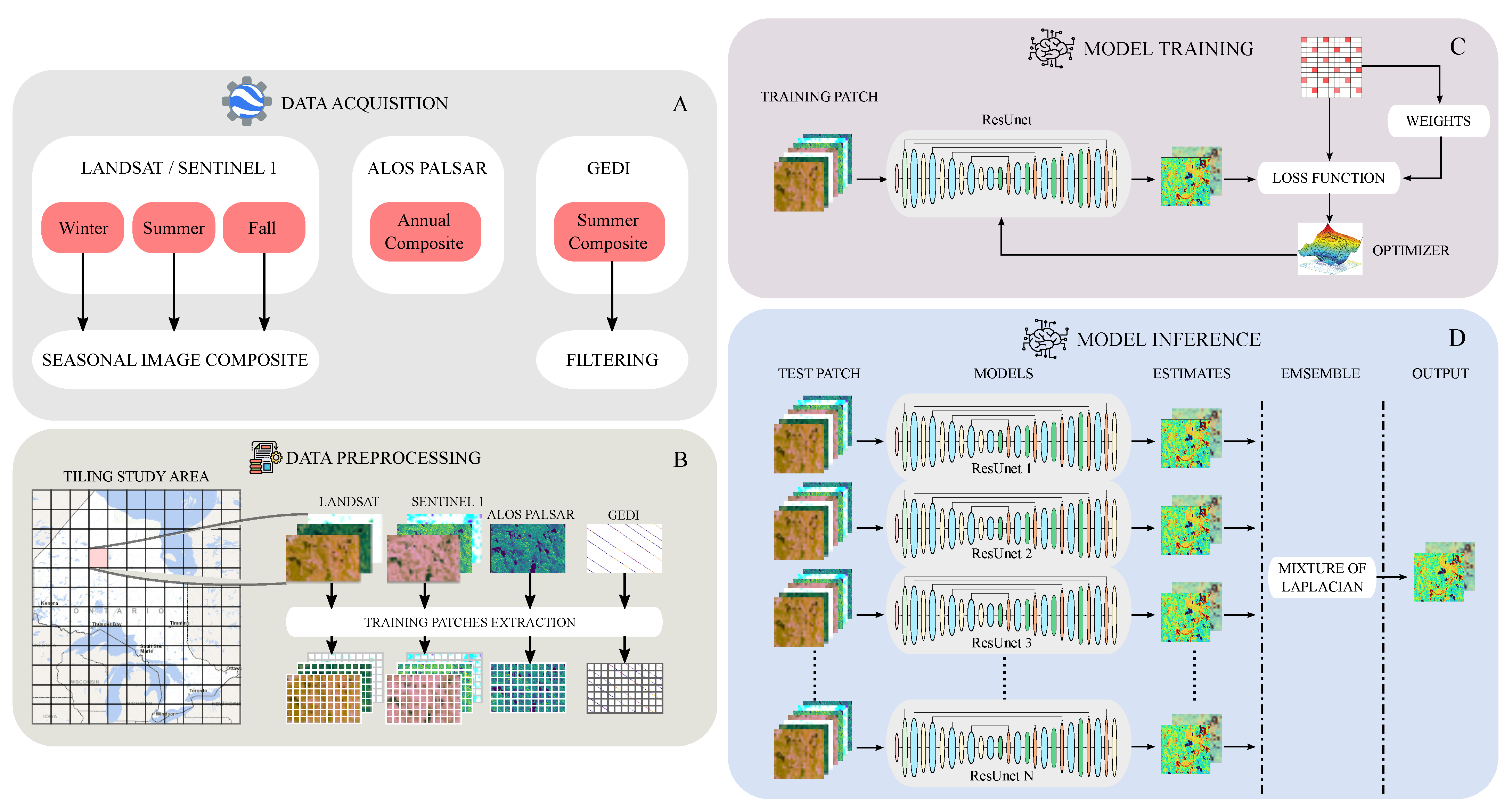
In this study, we estimate spatially continuous high-resolution canopy height and uncertainty using ensembles of deep learning (DL) regression models. As illustrated in Figure 4, our approach trains a fully convolutional neural network (FCN) [45] rooted in the ResUNet [46] architecture using data from Sentinel-1, Landsat 7 and 8, ALOS-PALSAR-2, and geographic coordinates as covariates to predict the GEDI RH98 canopy height across the study area (see Table 1).
Our methodology is divided into four stages: data acquisition, data preprocessing, model training, and model inference, as outlined in Figure 4. The data-acquisition stage collects remotely sensed data from the aforementioned satellite sources (Figure 4A), following the procedure outlined in Section 2.2.1. To reduce autocorrelation effects, we split the study area into non-overlapping regions during the data-preprocessing stage (Figure 4B), ensuring that the training and testing data are spatially independent. Within each region, we generate a dataset comprising coregistered patches extracted from all covariates and the target variable using a sliding window approach with overlap.
During the model-training stage, coregistered patches serve as input to the neural network, which is optimised to simultaneously predict both canopy height and the corresponding uncertainty at the pixel level (Figure 4C). To address different sources of uncertainty, we use an ensemble of neural networks, each trained on distinct subsets of the training and validation data from spatially independent regions. We use five ensemble members, consistent with prior probabilistic canopy-height frameworks [26,27] and with common deep-ensemble practice, for which a small ensemble of around five members already captures most of the predictive-uncertainty benefit, with diminishing returns for larger ensembles [47]. In the inference stage (Figure 4D), the ensemble is applied to generate final predictions for canopy height and associated uncertainty across the test regions. The subsequent sections elaborate on the model training procedure, the network architecture, and the methodology used to quantify uncertainty during inference.

2.3.1. Neural Network Architecture

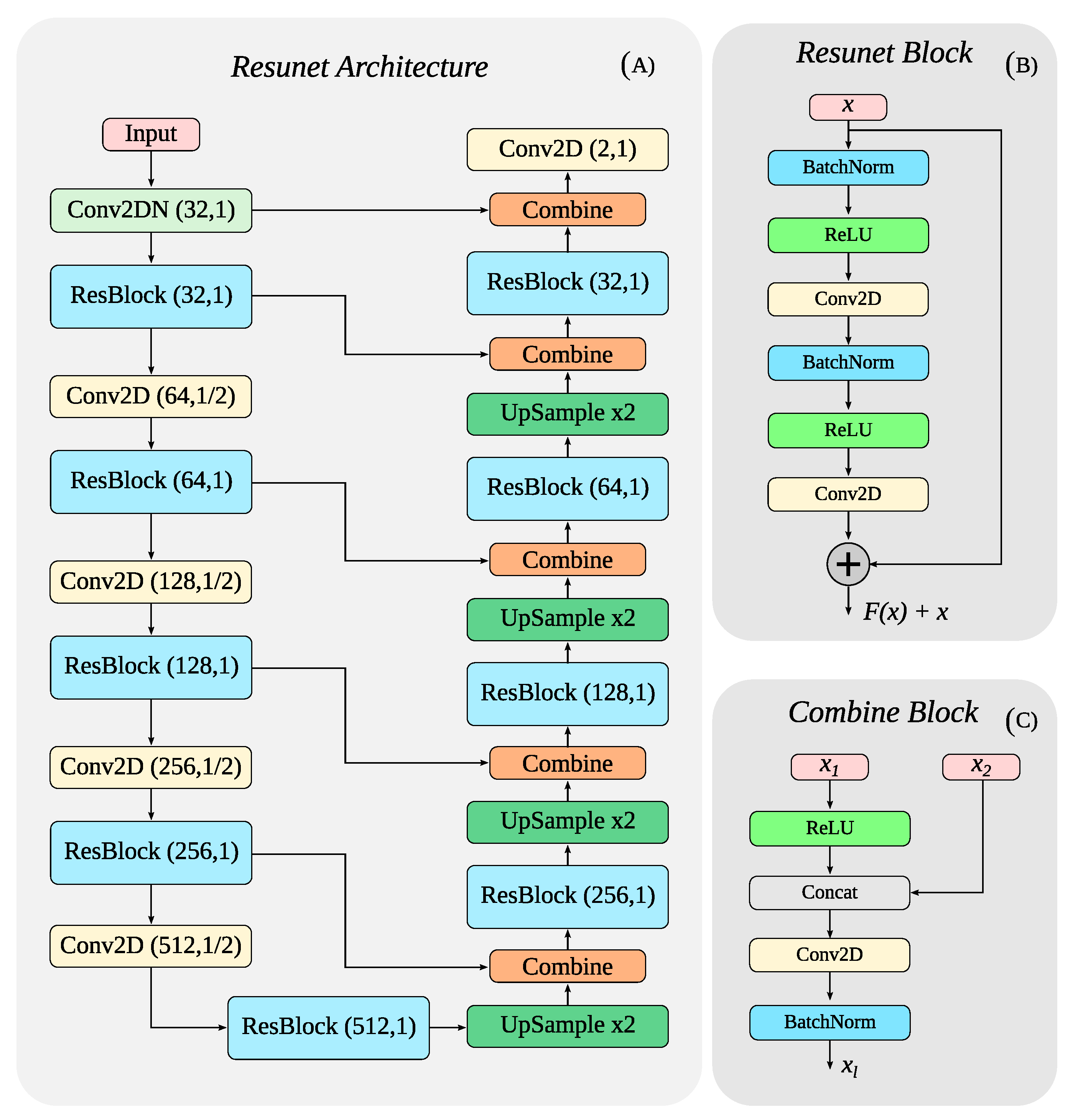
Figure 5 illustrates the neural network architecture employed in this study, which is a variation of the ResUNet-a model introduced by Diakogiannis et al. [46]. Compared to the original architecture, which uses multiple atrous [48] parallel convolution operations in the residual blocks (52 million parameters), our adaptation replaces these with traditional pre-activation residual blocks [49], reducing complexity to approximately 8.8 million trainable parameters. This reduction improves computational efficiency and makes the model less prone to overfitting, which is particularly important given the noise in GEDI training data from weather contamination and geolocation errors.
Our ResUNet architecture (Figure 5A) consists of an encoder–decoder structure with 5 resolution levels. The initial 1 × 1 convolution with batch normalisation [50] projects input features to 32 channels without spatial mixing, preserving fine-scale details at the network’s entry stage [46]. Each encoder stage doubles the channel count ( 32 64 128 256 512 ), with spatial downsampling performed via strided convolutions (stride 2). Residual projections use matching 1 × 1 convolutions to align dimensions when needed. The decoder mirrors this structure in reverse, using bilinear upsampling ( × 2 ) followed by a normed 1 × 1 convolution (Conv2DN) and residual blocks at each level [46]. Skip connections are implemented through combine blocks (Figure 5C) that concatenate encoder and decoder features and apply normed convolution to adjust the channel count. All residual blocks (Figure 5B) follow a pre-activation design, applying batch normalisation and ReLU before each of two 3 × 3 convolutions, with an additive shortcut connection. The final layer uses a 1 × 1 convolution to output 2 channels ( μ and b for the Laplace distribution). Input patches are 64 × 64 pixels with 26 feature channels (Table 1).

2.3.2. Model Setup and Parametrisation

Let S = { x ( i ) , y ( i ) } i = 0 N denote the set of observed data drawn from an unknown joint probability distribution J ( X , Y ) , where N is the total number of samples and the x ( i ) X , y ( i ) Y pair represents the covariates and the target variable. The goal is to approximate the underlying conditional probability distribution P ( Y X ) by learning a nonlinear regression function f θ : X Y through a neural network. In this scheme, each sample x ( i ) R w × w × c , y ( i ) R w × w × d pair corresponds to multidimensional coregistered square patches, where w denotes the spatial dimensions, c the number of input covariates, and d the number of target variables.
Similar to Nair et al. [51], we optimise the network parameters θ by minimising the Negative Log-Likelihood (NLL) loss of the Laplace distribution:
NLL = 1 N w 2 i = 1 N j , k V ( i ) N V ( i ) μ ^ j , k ( i ) y j , k ( i ) b ^ j , k ( i ) + log ( 2 b ^ j , k ( i ) ) ,
where μ ^ ( i ) and b ^ ( i ) denote the network’s expected-value and scale (uncertainty) estimates, respectively, for a given input sample x ( i ) . Here V ( i ) is the set of valid pixel coordinates in the GEDI map y ( i ) , and N V ( i ) is the associated number of valid pixels.
The network outputs a two-channel map y ^ i R h × w × 2 , where the first channel corresponds to the expected canopy height ( μ ^ ( i ) ) per pixel and the second channel corresponds to the associated uncertainty estimate ( b ^ ( i ) ). For a Laplace distribution, the variance is given by Var = 2 ( b ^ ( i ) ) 2 [52]. During training, since the GEDI reference data y ( i ) is sparse, we masked out pixels without observations using a coordinate matrix V ( i ) containing the locations of valid GEDI observations.
Since GEDI RH98 exhibits a skewed distribution with a long tail at high canopy heights, analogously to Yang et al. [53], Steininger et al. [54], we use a weighting function f ω ( y j , k ( i ) ) to improve model performance across the entire target domain. The weighting function adjusts the cost according to the inverse kernel density estimate (KDE) of the target variable distribution, such that rare height values are more heavily penalised than frequent ones. The resulting loss function is
NLL = 1 N w 2 i = 1 N j , k V ( i ) N V ( i ) f ω ( y j , k ( i ) ) μ ^ j , k ( i ) y j , k ( i ) b ^ j , k ( i ) + log ( 2 b ^ j , k ( i ) ) ,
with
f ω ( z ) = 1 M h m = 1 M K z z m h p ,
where M, K, h, and p denote the total number of data points, the kernel function, the bandwidth, and the power exponent controlling the reweighting intensity, respectively.
We optimise the neural network using the NLL of the Laplace distribution rather than the Gaussian distribution because the Laplace likelihood is more robust to outliers [51], thereby improving estimates of both canopy-height means and uncertainty statistics. The Laplace distribution is particularly well suited to our data: some GEDI samples exhibit inconsistencies with the intended target despite filtering for strong and high-quality beams, an issue widely reported in prior work [55,56,57] and often attributed to weather effects (e.g., cloud contamination), transitions between forest and non-forest, or geolocation inaccuracies.

2.3.3. Uncertainty Estimation and Calibration

Analogously to Lang et al. [26], our approach employs ensembles of neural networks to characterise both aleatoric and epistemic uncertainty (Figure 4). Each model in the ensemble outputs a Laplace ( μ ^ , b ^ x ) distribution, as described in Section 2.3.2. The b ^ estimates allow each model to capture inherent data uncertainty (aleatoric), arising from both the covariates and the GEDI observations and influenced by sensor limitations, weather conditions, or geolocation errors. Variability across ensemble predictions reflects the epistemic uncertainty: high agreement among the models corresponds to low epistemic uncertainty, whereas large discrepancies indicate high epistemic uncertainty.
The ensemble’s output derived from the mixture of distributions is
p ( y x ) = e = 1 N e π e ( x ) · Lap ( y μ ^ e ( x ) , b ^ e ( x ) ) ,
where π e ( x ) , e = 1 , 2 , , N e are the mixing probabilities with π e ( x ) 0 and e = 1 N e π e ( x ) = 1 , and N e denotes the number of models in the ensemble. Each component Lap ( y μ ^ e ( x ) , b ^ e ( x ) ) is a Laplace distribution with location parameter μ ^ e ( x ) and scale parameter b ^ e ( x ) predicted by ensemble member e given input x.
The total mean (first moment) and total variance (second moment) of the ensemble distribution are
E [ Y ] = μ = e = 1 N e π e μ ^ e ,
E [ ( Y μ ) 2 ] = σ 2 = e = 1 N e π e ( σ ^ e 2 + μ ^ e 2 ) e = 1 N e π e μ ^ e 2 = e = 1 N e π e σ ^ e 2 + e = 1 N e π e μ ^ e 2 e = 1 N e π e μ ^ e 2 .
Assuming equal mixing probabilities π e = 1 / N e and using the Laplace variance σ ^ e 2 = 2 b ^ e 2 , we obtain
E [ ( Y μ ) 2 ] = 2 N e e = 1 N e b ^ e 2 aleatoric + 1 N e e = 1 N e μ ^ e 2 1 N e e = 1 N e μ ^ e 2 epistemic ,
where the first term captures the mean aleatoric uncertainty (average within-model variance) and the second term captures the epistemic uncertainty (between-model disagreement).
The total uncertainty quantified above is not necessarily well-calibrated [58,59,60,61]. Calibration refers to the alignment between the model’s predicted uncertainties and their actual reliability [62]: a well-calibrated model exhibits a linear relationship between predicted uncertainty and observed prediction error [58,59,60]. Among the available calibration approaches, we adopt the Platt-based [63] scaling strategy adapted for regression by Laves et al. [58,59], Kuleshov et al. [60], because it does not modify the predictive mean of the model and only adjusts the uncertainty estimates. We apply the procedure to the total uncertainty coming from the mixture of Laplace distributions.
Formally, a well-calibrated estimation of predictive uncertainty for a regression model satisfies
E x , y y y ^ 2 Σ ^ 2 = Σ 2 = Σ 2 , Σ 2 R 0 ,
where Σ 2 denotes the total uncertainty. To calibrate the model’s uncertainty Σ ^ 2 , we apply the affine transformation σ cal = a · σ ^ + b , where σ ^ = Σ ^ 2 is the raw ensemble standard deviation and a, b are calibration parameters optimised by minimising the uncertainty calibration error (UCE)—the weighted mean absolute difference between predicted uncertainty and observed RMSE across binned uncertainty intervals. To avoid optimistic calibration, within each of the five cross-validation folds the held-out test tiles were split into disjoint calibration and evaluation subsets: a and b were fit on the calibration subset—disjoint from both the network-training samples and the evaluation samples—and all reported uncertainty metrics were computed on the evaluation subset. The fitted parameters and the resulting calibration error are reported in the uncertainty analysis (Section 3.8). This affine formulation extends the single-scalar approach of Laves et al. [58,59] to better accommodate the shift and scaling mismatch commonly observed in deep-ensemble uncertainty estimates, while preserving the model’s predictive performance.

2.4. Experimental Design

The study area was divided into a regular 10 × 10 grid of 100 non-overlapping tiles, each approximately 240 × 210 km ( 8000 × 7000 pixels at 30 m), spanning Ontario’s bounding box in the EASE-Grid 2.0 North projection. Of the 100 tiles, 71 intersect GEDI coverage and enter model development, while the 29 without GEDI observations are reserved for wall-to-wall inference. Of the 71, the 26 that also intersect the FRI ALS footprint carry the independent ALS validation reference, and the other 45 carry GEDI supervision without an ALS reference. These tile dimensions are orders of magnitude larger than the autocorrelation ranges reported for forest-structure variables (typically hundreds of metres to a few kilometres at the stand-to-landscape scale [64,65]), so any residual correlation between a training tile and an adjacent held-out tile is confined to a thin boundary zone and is small relative to the tile area, limiting leakage between training and validation [66,67].
Five-fold spatial cross-validation was performed at the tile level over the 71 GEDI-covered tiles, under an 80/20 (train/test) scheme: in each fold, about 80% of the tiles were used for training and the remaining 20% for testing, with the same partition reused across all experimental configurations so that performance differences reflect modelling choices rather than partition variability. The fold assignment and the resulting tile roles are shown in Figure S1b, and evaluation metrics were computed on the held-out tiles that intersect the ALS footprint. Within each fold, the training tiles were split into five mutually exclusive spatial subsets, and one ensemble member was trained on each; the held-out test set is common to all five members, whose outputs are combined through the mixture of Laplace distributions (or Gaussian, for the baseline comparison) described in Section 2.3.3.
To reduce the potential impact of artefacts during training, extreme covariate values were clipped to the interval ( μ 3 σ , μ + 3 σ ) , where μ and σ denote the empirical covariate mean and standard deviation. Given the large dataset, we adopted an online computation strategy using the algorithm of Chan et al. [68] as implemented in scikit-learn [69]. Standard normalisation was then applied to facilitate network optimisation [70].
Training samples were generated by extracting coregistered 64 × 64 -pixel patches (∼1.9 km × 1.9 km at 30 m) from all sensors for each year and tile, using a sliding window with 25% overlap across regions containing GEDI observations. The patch size is the smallest area that contains a sufficient number of GEDI footprints given the sensor’s along-track (∼60 m) and across-track (∼600 m) sampling pattern. Patches containing fewer than 1% valid GEDI pixels (∼41 of the 4096 patch pixels) were discarded; this threshold was set during preliminary experiments to balance two competing requirements—retaining enough patches to span the study domain, while ensuring each patch carries enough supervised pixels for the masked NLL gradient to be meaningfully informative. Patch extraction is confined within tile boundaries, so 25% overlap never crosses fold boundaries. Patches were exported to TFRecords for efficient I/O during training [71]. In total, the dataset comprised approximately 19.85 million valid GEDI pixels across both years: 9,070,221 from 2019 and 10,780,180 from 2020.
During training, we computed the GEDI sample-density distribution for each run, randomly sampling 10 million samples from the training set. We then estimated the KDE-based sample weights using label distribution smoothing (LDS) with a Gaussian kernel of size 5 and standard deviation σ = 2 , and applied power-inverse reweighting with exponent p = 0.8 , which moderates the reweighting intensity to avoid over-penalising extremely rare height values while still upweighting underrepresented tall-canopy samples. Network weights were initialised using the HeNormal truncated normal distribution and regularised with L2 weight decay ( 10 5 ). We used the Adam [72] optimiser, with learning rate 10 4 on a cosine annealing schedule [73], gradient clipping to norm 1.0, batch size 256, and 50 epochs. All experiments were conducted on Digital Research Alliance of Canada (formerly Compute Canada) infrastructure using NVIDIA H100 GPUs (40 GB VRAM), 4 CPU cores, and 64 GB RAM per job. Each experiment required approximately 30 h of training on average.
We ablated three input factors to quantify their contributions: (i) temporal coverage—seasonal composites (winter–summer–fall, W–S–F) versus a single summer-only composite (X–S–X); (ii) sensor inputs—Landsat (LS), Sentinel-1 (S1), and ALOS-PALSAR-2 (AP), used individually and in combination; and (iii) geographic information—latitude/longitude (LL) included or excluded (X). Configurations are labelled by concatenating the temporal pattern and the sensor/geographic pattern, with X marking an omitted input (e.g., W–S–F LS–S1–AP–X denotes seasonal composites of all three sensors without coordinates); the naming convention is summarised in Table 3. We also trained loss × weighting variants of the reference configuration—Gaussian versus Laplace NLL, each with and without the KDE inverse-density weighting—to separate the effects of the likelihood and the sample weighting.
Model accuracy was evaluated against the spatially aggregated ALS canopy-height reference at the 98th percentile, with GEDI itself and the four global products serving as comparison benchmarks. To support a comprehensive evaluation, the validation pool aggregates GEDI ∩ ALS intersection samples from both 2019 and 2020, pairing each GEDI shot with the ALS tile of the same calendar year where possible. Performance is summarised using R 2 , RMSE, MAE, bias (predicted − observed), and the slope of the predicted-versus-observed regression line. To assess how performance varies with forest composition, we stratified the GEDI ∩ ALS validation samples using the 2020 North American Land Cover map (NALCMS, 30 m) [38] into four classes: coniferous, deciduous, mixedwood (stands with intermingled deciduous and coniferous species), and treed-wetland. This stratification supports a forest-type-resolved view of how seasonal and sensor contributions interact with canopy composition.

3. Results

3.1. Agreement Between GEDI RH98 and ALS-Derived Metrics

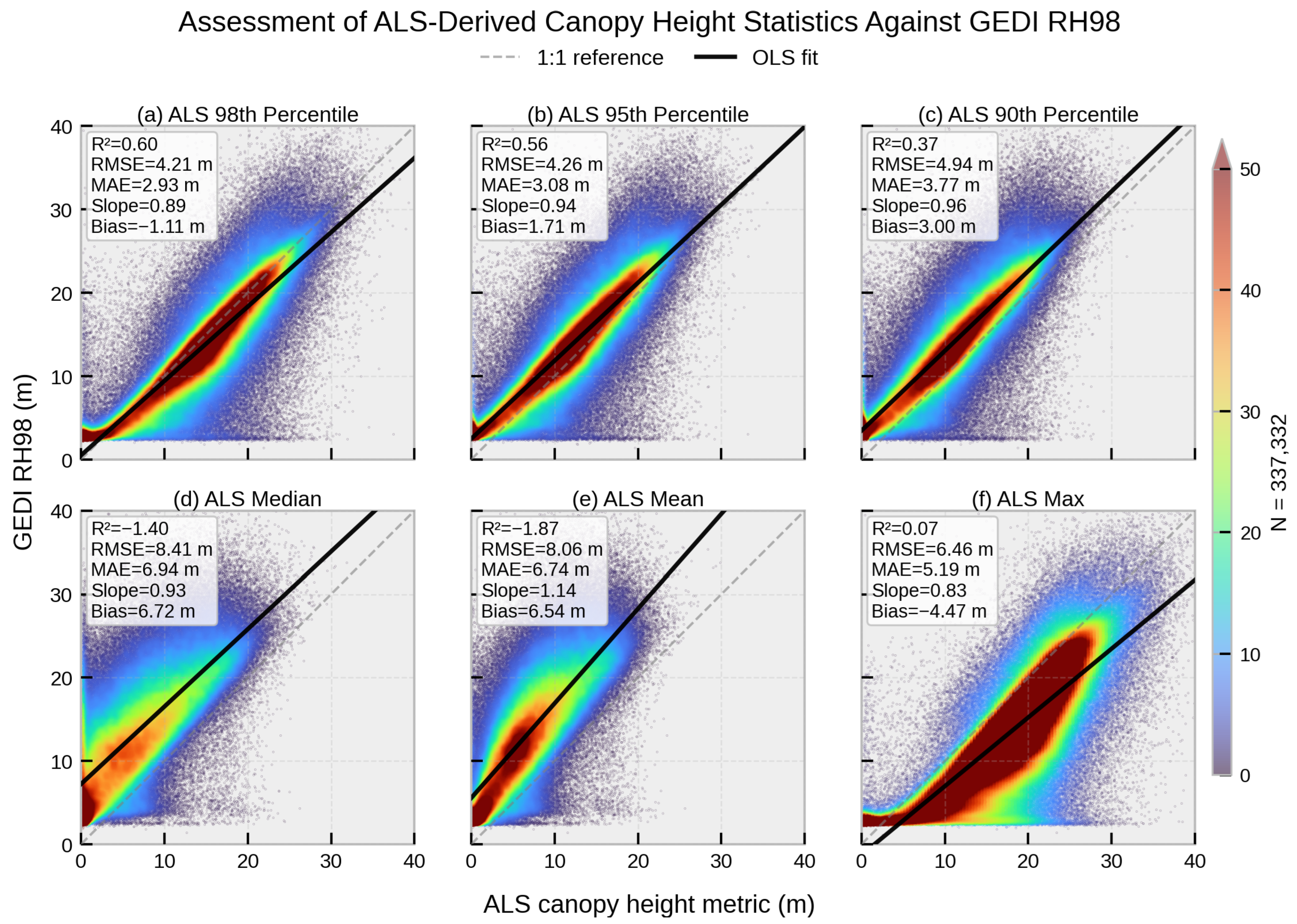
We first established which ALS-derived height statistic should serve as the reference for subsequent comparisons. Using 337,332 spatially co-located footprints (Figure 6), GEDI RH98 was compared against six ALS-derived statistics (98th, 95th, 90th percentiles; median; mean; maximum). The 98th percentile produced the strongest agreement with GEDI RH98 ( R 2 = 0.60 , RMSE = 4.21 m, MAE = 2.93 m, bias = −1.11 m), and its regression slope of 0.89 indicates that GEDI RH98 systematically underestimates ALS P98 at taller heights. The remaining statistics performed substantially worse: 95th percentile ( R 2 = 0.56 , RMSE = 4.26 m, bias = 1.71 m), 90th percentile ( R 2 = 0.37 , RMSE = 4.94 m, bias = 3.00 m), median ( R 2 = 1.40 , RMSE = 8.41 m, bias = 6.72 m), mean ( R 2 = 1.87 , RMSE = 8.06 m, bias = 6.54 m), and maximum ( R 2 = 0.07 , RMSE = 6.46 m, bias = −4.47 m). These results justify the choice of ALS P98 as the reference statistic for the remainder of the paper while flagging the residual GEDI–ALS bias as a known systematic component that must be considered when interpreting model performance.

3.2. Effect of the Laplace vs. Gaussian Negative Log-Likelihood Loss

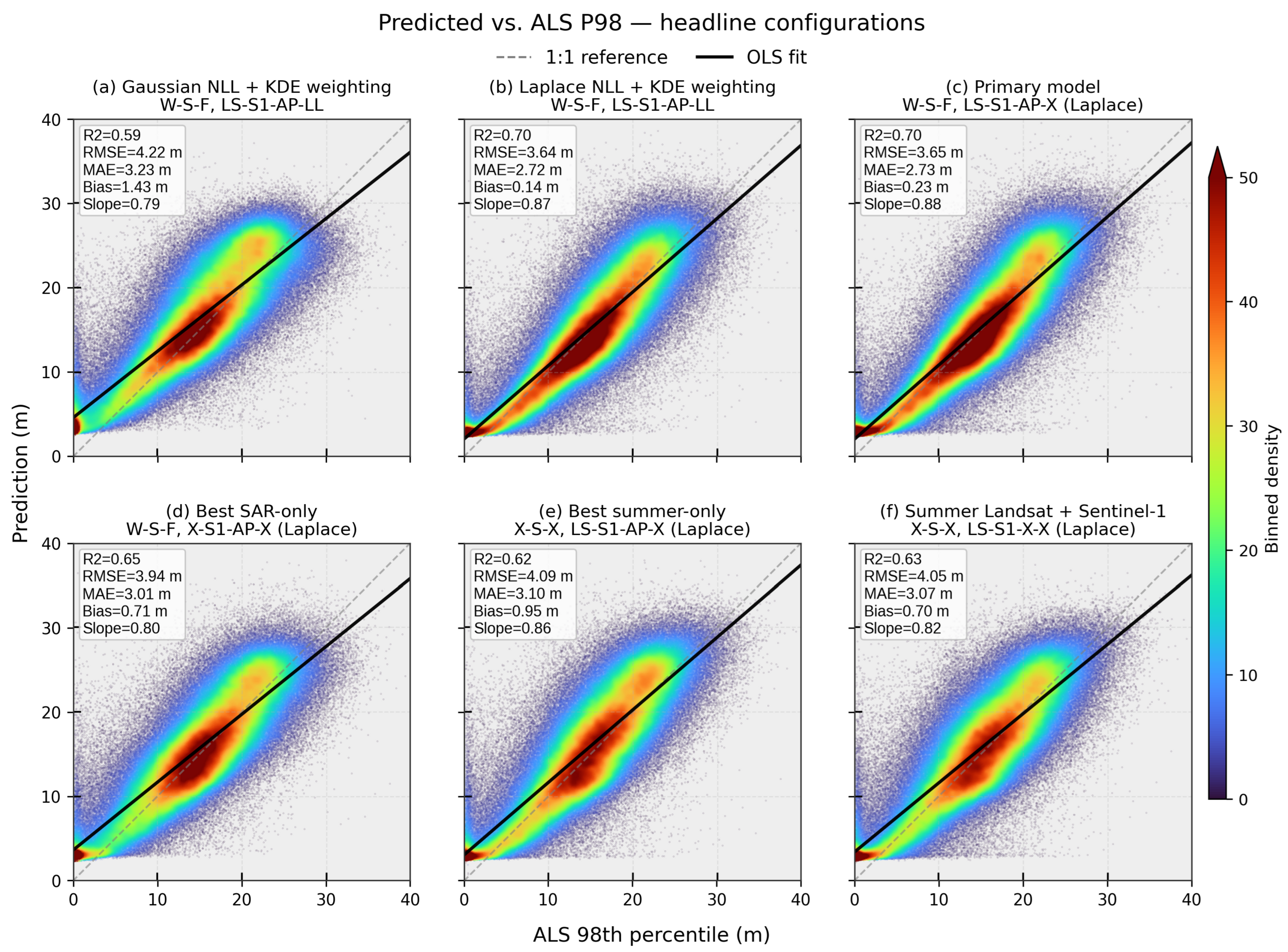
To isolate the contribution of the Laplace NLL loss, two models were trained with the same architecture and input configuration (W–S–F, LS–S1–AP–LL), differing only in the choice of NLL distribution. The Laplace-based model achieved R 2 = 0.70 , RMSE = 3.64 m, MAE = 2.72 m, and bias = 0.14 m, compared with R 2 = 0.59 , RMSE = 4.22 m, MAE = 3.23 m, and bias = 1.43 m under Gaussian NLL (Figure 7a,b)—improvements of 18.6% in R 2 , 13.7% in RMSE, and 15.8% in MAE. The systematic bias was reduced by an order of magnitude, from 1.43 m to 0.14 m, consistent with the Laplace likelihood’s heavier-tailed behaviour, which down-weights outlier GEDI labels rather than letting them drag the conditional mean. All subsequent results use the Laplace NLL loss.
The two models were trained with identical hyperparameters—the same Adam optimiser, learning rate ( 10 4 ), cosine-annealing schedule, gradient clipping, batch size (256), 50-epoch budget, and KDE-based inverse-density sample weighting (Section 2.3.2)—and the Laplace likelihood required no loss-specific re-tuning of the learning rate. The scale output b ^ was mapped to the strictly positive domain before entering the NLL, removing the need for a scale initialisation; both variants converged within the same 50-epoch budget.
We also trained both losses without density weighting, isolating the weighting from the likelihood (Supplementary Figure S3). The Laplace RMSE stays below the Gaussian RMSE both with and without weighting (by 0.58 m and 0.33 m, respectively), so the robustness gain follows from the likelihood. Removing the weighting lowers the aggregate RMSE (by 4.4% for Laplace and 9.7% for Gaussian) and raises R 2 —metrics dominated by the abundant mid-height canopies that the weighting down-weights—but turns the bias negative—flipping the near-zero Laplace bias (0.14 m) to a marked underestimation ( 1.40 m) and the positive Gaussian bias (1.43 m) to 1.22 m—and lowers the slope, as tall canopies are no longer up-weighted and predictions saturate above ∼25 m.

3.3. Overall Canopy-Height Estimation Performance

Figure 7, Figure S4 and Figure S5 summarise the performance of the Laplace-based configurations against the ALS P98 reference; the main text highlights the headline models, while the full set of optical-containing ablations and SAR-only configurations is provided in the Supplementary Materials. Two configurations tied for best overall accuracy, W–S–F LS–S1–AP–X ( R 2 = 0.70 , RMSE = 3.65 m, MAE = 2.73 m, bias = 0.23 m, slope = 0.88) and W–S–F LS–S1–AP–LL ( R 2 = 0.70 , RMSE = 3.64 m, MAE = 2.72 m, bias = 0.14 m, slope = 0.87), the latter being marginally better on MAE/bias. Given the negligible accuracy difference and the risk of inducing spatial-autocorrelation artefacts when explicit coordinates are added to a model trained and tested within a single province, we adopt the coordinate-free variant LS–S1–AP–X as the primary configuration in all subsequent comparisons. Relative to GEDI itself (Figure 6a), LS–S1–AP–X improves explained variance ( R 2 = 0.70 vs. 0.60), MAE (2.73 m vs. 2.93 m), RMSE (3.65 m vs. 4.21 m), and absolute bias (0.23 m vs. 1.11 m), at the cost of a slightly lower slope (0.88 vs. 0.89). Both GEDI and the model are evaluated against the ALS P98 reference at the same co-located GEDI footprints. Table 4 consolidates R 2 , RMSE, MAE, bias, and slope for every model configuration, GEDI, and the four global products.
Within the seasonal (W–S–F) optical-containing family (Figure 7 and Figure S4), the primary model is robust to the removal of secondary inputs: dropping ALOS-PALSAR-2 while retaining coordinates (LS–S1–X–LL) increases RMSE by only 0.55% and reduces R 2 by 1.43%, and dropping both (LS–S1–X–X) increases RMSE by 2.47% and reduces R 2 by 2.86%. These small, non-compounding penalties indicate that the Landsat + Sentinel-1 seasonal pair carries most of the predictive signal, with ALOS-PALSAR-2 contributing incremental improvement.
SAR-only configurations (Figure S5; Table 4) show a larger but still moderate degradation relative to optical-containing models. The best SAR-only configuration (W–S–F, X–S1–AP–X) reaches R 2 = 0.65 and RMSE = 3.94 m, a 7.95% increase in RMSE and 7.14% decrease in R 2 relative to LS–S1–AP–X. Adding coordinates (X–S1–AP–LL) does not help ( R 2 = 0.64 , RMSE = 3.95 m), reinforcing the earlier observation that explicit location features add no value in a province-scale model. Single-sensor configurations degrade most sharply in both the optical-containing and SAR-only groups, confirming that multi-sensor fusion is the dominant lever on overall accuracy.

3.4. Contribution of Seasonal Observations

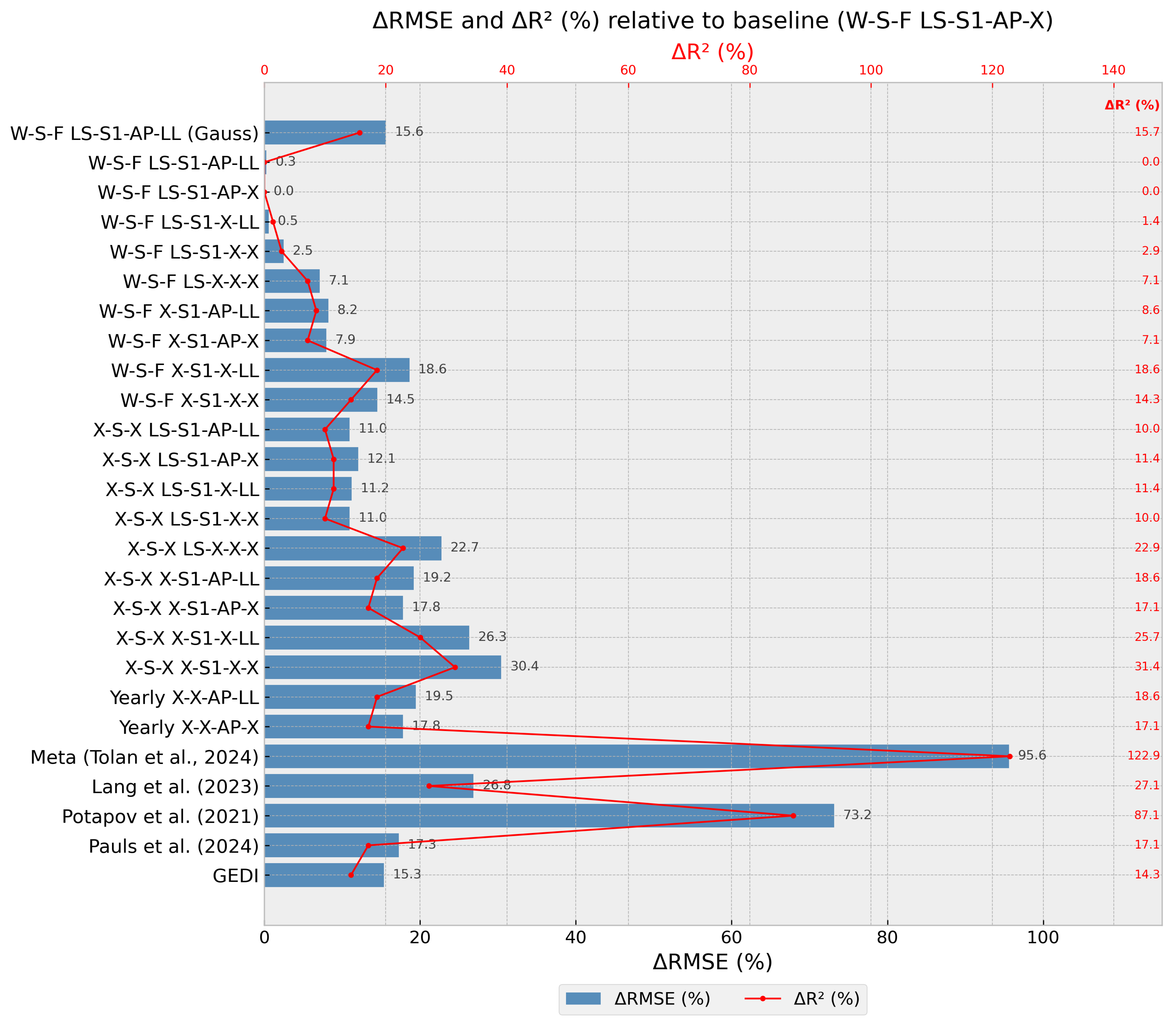
Removing seasonal information consistently degraded performance across every sensor configuration tested (Figure 7, Figure S4 and Figure 8). Relative to the primary model (W–S–F, LS–S1–AP–X), summer-only counterparts showed RMSE increases of 11.0–30.4% and R 2 declines of 10.0–31.4%, with the gap widening as the input set thinned. Summer-only Sentinel-1 without ALOS-PALSAR-2 fared worst: X–S1–X–X increased RMSE by 30.4% and reduced R 2 by 31.4%, followed by X–S1–X–LL (+26.3% RMSE, −25.7% R 2 ) and LS–X–X–X (+22.7% RMSE, −22.9% R 2 ). Adding a second summer sensor partially recovers performance: LS–S1–X–X stabilises at +11.0% RMSE and −10.0% R 2 , confirming that multi-sensor fusion compensates for the loss of phenological diversity even when only summer observations are available.
The matched-sensor comparison isolates the seasonal effect most cleanly (Table 4). The matched summer-only configuration (X–S–X, LS–S1–AP–X) reaches R 2 = 0.62 , RMSE = 4.09 m, MAE = 3.10 m, bias = 0.95 m, and slope = 0.86, whereas its seasonal counterpart with the same sensors achieves R 2 = 0.70 , RMSE = 3.65 m, MAE = 2.73 m, bias = 0.23 m, and slope = 0.88. Seasonal compositing therefore yields a 12.9% gain in R 2 , a 10.8% reduction in RMSE, and a fourfold reduction in bias, with no change in input sensors. Within the seasonal family itself, dropping individual sensors causes only modest penalties (W–S–F LS–X–X–X: +7.1% RMSE, −7.1% R 2 ; W–S–F X–S1–AP–LL: +8.2% RMSE, −8.6% R 2 ), and the largest in-family penalties occur for seasonal SAR-only configurations without ALOS-PALSAR-2 (W–S–F X–S1–X–LL: +18.6% RMSE, −18.6% R 2 ; W–S–F X–S1–X–X: +14.5% RMSE, −14.3% R 2 ).
Seasonal models also produced more uniform error behaviour across the full canopy-height range (Figure 7 and Figure S4). Their predicted-versus-observed densities track the 1:1 line more closely above 25 m, indicating reduced saturation in tall canopies, and they show smaller systematic offsets at the low end relative to summer-only configurations. The contrast is sharpest for single-sensor summer models, which exhibit the highest dispersion, the largest biases, and the lowest slopes in the entire experimental matrix.

3.5. Contribution of Multi-Sensor Fusion

Among the three sensors examined, Sentinel-1 emerges as the single most influential input: its removal damages performance more than the removal of ALOS-PALSAR-2 or coordinates (Figure 7 and Figure S5). Models pairing Landsat with Sentinel-1 retain strong performance, while seasonal Sentinel-1 alone benefits substantially from adding ALOS-PALSAR-2: configurations X–S1–AP–X and X–S1–AP–LL reach accuracies comparable to the seasonal Landsat-only model (LS–X–X–X) and clearly exceed summer SAR-only configurations. The seasonal SAR-fusion model (W–S–F, X–S1–AP–X; R 2 = 0.65 , RMSE = 3.94 m) outperforms the summer Landsat + Sentinel-1 model (X–S–X LS–S1–X–X; R 2 = 0.63 , RMSE = 4.05 m), demonstrating that adding seasonality to SAR can compensate for the absence of optical inputs (Table 4).
Among the weakest configurations are the summer single-sensor Sentinel-1 models (X–S1–X–X: R 2 = 0.48 , RMSE = 4.76 m; X–S1–X–LL: R 2 = 0.52 , RMSE = 4.61 m). Within single-sensor summer experiments, Landsat alone ( R 2 = 0.54 ) outperforms Sentinel-1 alone ( R 2 = 0.48 ). The yearly ALOS-PALSAR-2 composite (X–X–AP–X; R 2 = 0.58 , RMSE = 4.30 m) outperforms both summer single-sensor cases, but lags the primary model by 17.8% in RMSE and 17.1% in R 2 (Figure 8).

3.6. Comparison with GEDI Observations and Global Canopy-Height Products

GEDI itself produced the highest predicted–observed slope (0.89) among all comparisons (Figure 6), confirming the spatial aggregation methodology. GEDI also exhibited the largest tails: shots above 30 m where ALS P98 is below 5 m, and shots reporting low values over tall ALS reference canopies. A dense cluster near the origin of Figure 6a shows GEDI systematically overestimating canopy height where ALS P98 is below 5 m, a pattern that persists, in attenuated form, across all trained model configurations (Figure 7 and Figure S5). The persistence of this low-range overestimation in the model outputs indicates that it is inherited from the GEDI training labels rather than introduced by the model architecture; the high-range outliers, in contrast, are largely absorbed by the Laplace likelihood and the seasonal multi-sensor inputs.
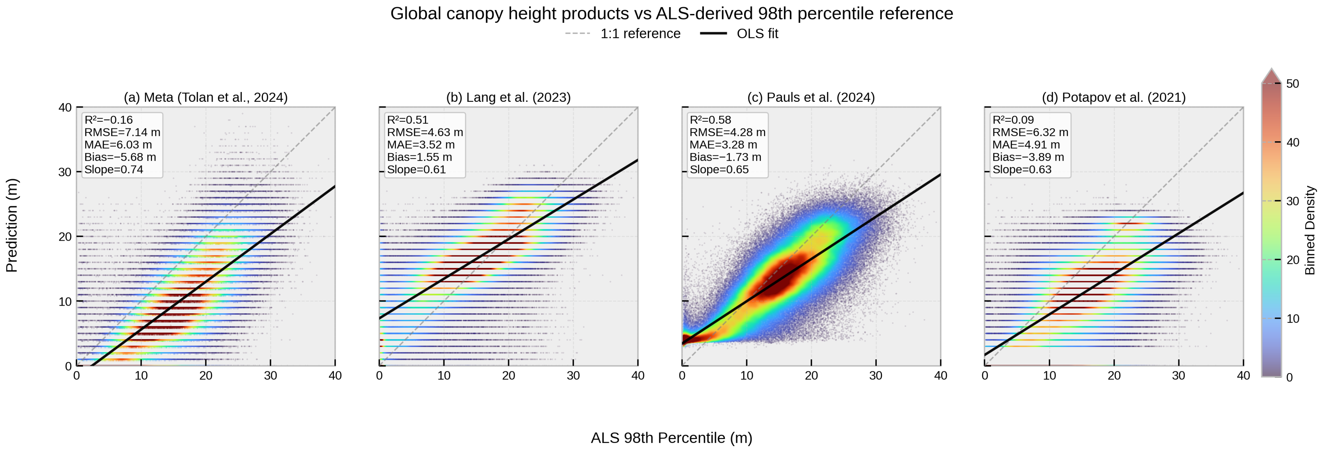
All four global products underperform our regional models within the Ontario test domain (Figure 9; Table 4). Meta [30] shows the lowest accuracy ( R 2 = 0.16 , RMSE = 7.14 m, MAE = 6.03 m, bias = −5.68 m); Potapov et al. [21] is similar ( R 2 = 0.09 , RMSE = 6.32 m, MAE = 4.91 m, bias = −3.89 m). Both compress the predicted height range with a strong negative bias, indicating limited ability to reproduce local canopy-height variation. Lang et al. [27] improves on explained variance ( R 2 = 0.51 , RMSE = 4.63 m, MAE = 3.52 m, bias = 1.55 m) but has the lowest slope (0.61) of the four products. Pauls et al. [28] is the strongest of the global products ( R 2 = 0.58 , RMSE = 4.28 m, MAE = 3.28 m, bias = −1.73 m, slope = 0.65), with a denser predictive core close to the ALS reference.

3.7. Prediction Error Along Canopy Heights

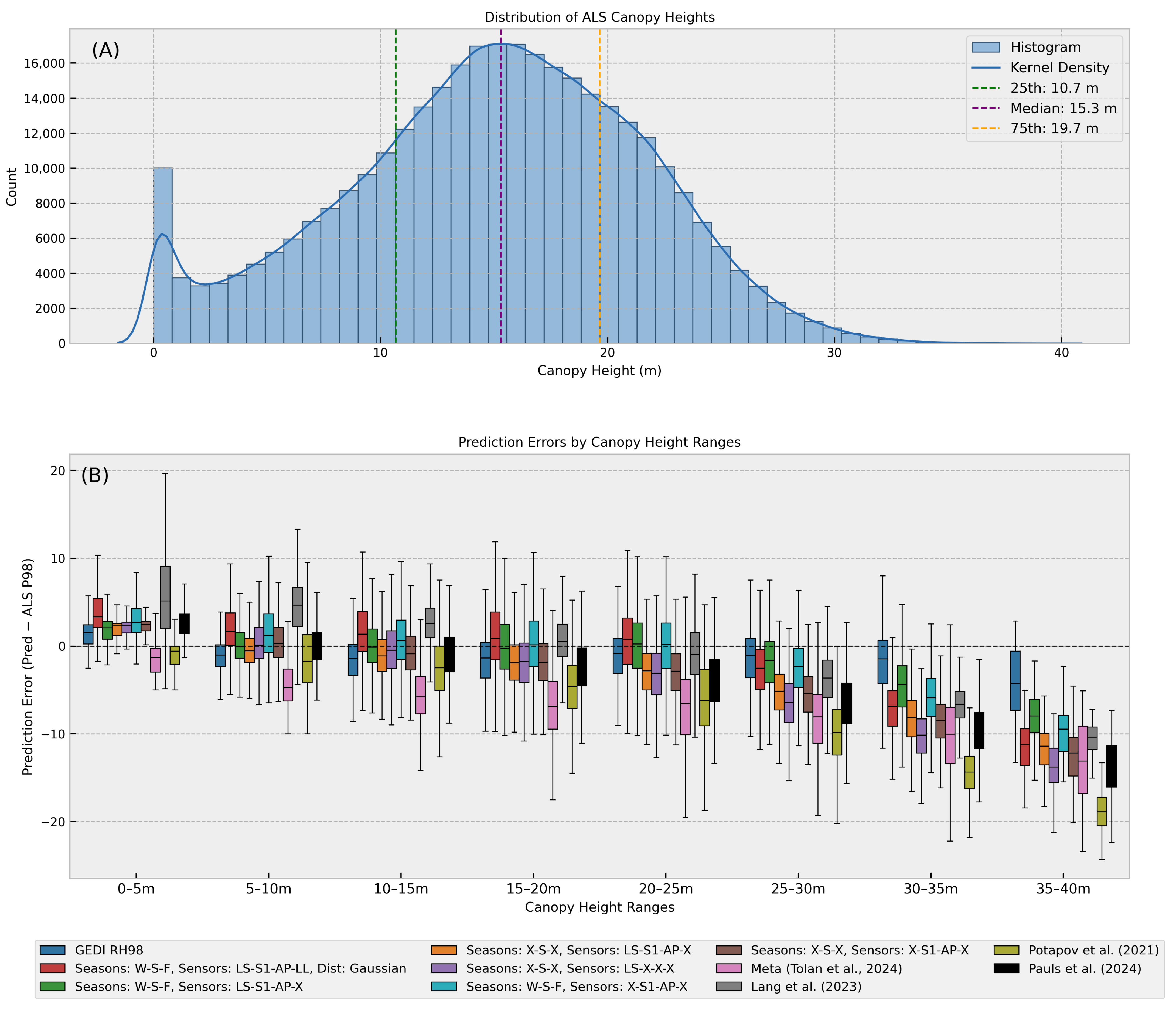
Figure 10A shows the distribution of ALS reference canopy heights across the 0–40 m range. The distribution is right-skewed, with a median of 15.3 m (25th–75th percentile: 10.7–19.7 m) and a long tail toward taller canopies. Figure 10B presents boxplots of prediction error in 5 m canopy-height bins for GEDI, selected model configurations, and the four global products. GEDI itself shows minimal systematic bias across most bins, with wider whiskers in taller canopy ranges. Among the trained models, the primary configuration (W–S–F LS–S1–AP–X) delivers the most balanced performance: underestimation only emerges above 25 m, the saturation effect is the smallest of any configuration tested, and the 0–5 m bin is improved relative to GEDI, where GEDI tends to overestimate.
The Gaussian baseline (W–S–F LS–S1–AP–LL, Gaussian) shows wider error dispersion and more pronounced underestimation in tall canopies than its Laplace counterpart, confirming the robustness advantage of the Laplace loss. Summer-only multi-sensor models (X–S–X LS–S1–AP–X) underestimate more sharply above 20 m, and the summer Landsat-only model (X–S–X LS–X–X–X) saturates earlier with pronounced underestimation above 20–25 m. The seasonal SAR-fusion model (W–S–F X–S1–AP–X) outperforms the summer optical-only configuration in tall canopies, supporting the role of SAR for vertical-structure retrieval, while the summer SAR-fusion configuration (X–S–X X–S1–AP–X) lies between its seasonal counterpart and the summer optical-only configuration.
Among the global products, Meta displayed the most pronounced and consistent underestimation across all height intervals, with the widest error dispersions. Potapov et al. [21] followed a similar pattern with slightly less bias and narrower dispersion. Lang et al. [27] exhibited a distinct trend reversal: overestimation below 15 m shifting to underestimation beyond 25 m. Pauls et al. [28] showed the most stable performance of the four, with minimal error in low canopy ranges and moderate underestimation appearing above 20 m.

3.8. Uncertainty Analysis

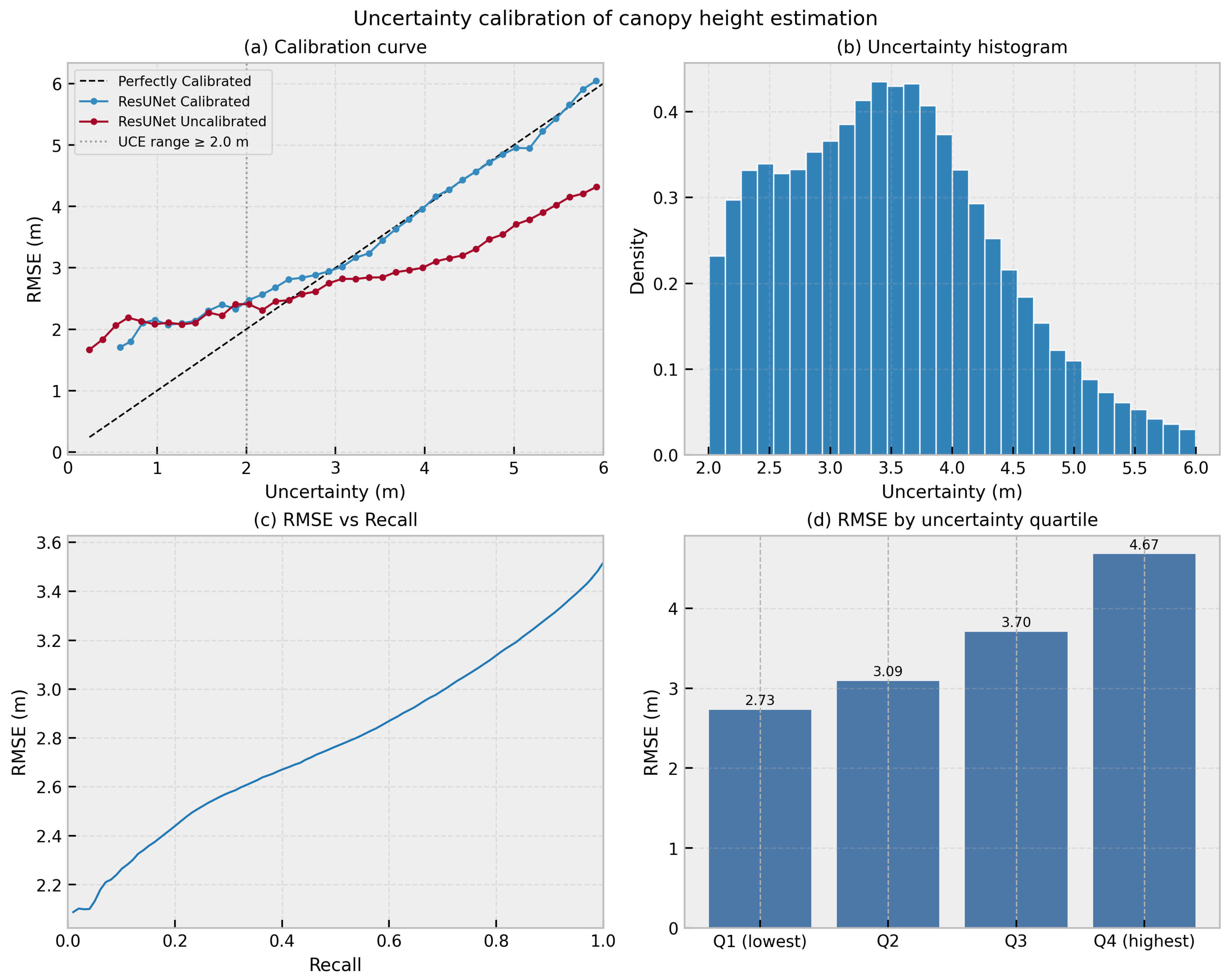
Figure 11a shows calibration curves for the primary model (W–S–F, LS–S1–AP–X) before and after Platt-style affine scaling. The raw ensemble is overconfident: in the low-uncertainty regime (<1.5 m predicted), the empirical RMSE is 2.0–2.2 m, and the uncalibrated curve sits well above the 1:1 line across the lower range. After applying the affine transformation σ cal = a · σ raw + b , the calibrated curve tracks the 1:1 line closely from ∼2 m upward, indicating that the post hoc calibration aligns predicted uncertainty with observed error without modifying the predictive mean. The affine scaling reduced the uncertainty calibration error (UCE) by roughly an order of magnitude, from 1.12 m for the raw ensemble to 0.10 m for the calibrated uncertainty (evaluated over the ≥2 m range), with fitted parameters a = 0.65 and b = 0.47 m.
The residual overconfidence below ∼2 m predicted uncertainty is concentrated in homogeneous forest interiors, where ensemble members agree strongly while the GEDI-inherited label noise imposes an error floor of ∼2.0–2.2 m; the calibration raises these estimates but does not fully close this gap. This regime comprises 12.1% of the validation footprints, over which the empirical RMSE (2.29 m) still exceeds the mean calibrated uncertainty (1.34 m), and it is concentrated in the 0–5 m canopy range (empirical RMSE 2.09 m against a mean calibrated uncertainty of 1.11 m)—the same low-canopy stratum where GEDI overestimates (Section 3.7). Calibrated uncertainties at the ∼2 m floor should therefore be read as a lower bound on true error in these strata.
We quantified how the calibrated per-pixel uncertainty relates to canopy structure using Spearman rank correlations against two references: (i) the predicted canopy height, as a measure of canopy magnitude, and (ii) local structural heterogeneity. Because the model ingests 30 m composites, heterogeneity was defined at the 30 m scale at which the model operates: the ALS canopy-height model was aggregated to a 30 m 98th-percentile grid, a focal (moving-window) standard deviation was computed over a 3 × 3 (90 m) window, and this neighbourhood heterogeneity was sampled at each of the GEDI ∩ ALS validation footprints. Across these footprints, calibrated uncertainty increased with predicted canopy height (Spearman ρ = 0.57 ) and, independently, with local structural heterogeneity ( ρ = 0.46 ; partial ρ = 0.48 after controlling for canopy height, and ρ = 0.45 for a 5 × 5 , 150 m window). Because the association with heterogeneity is essentially undiminished when canopy height is held constant, the confidence layer carries information about structural difficulty beyond canopy magnitude, consistent with the spatial pattern in Figure 12, where uncertainty is elevated along forest edges and land-cover transitions.
The distribution of calibrated uncertainty (Figure 11b) is approximately bell-shaped, concentrated between 2.5 and 5.0 m with a peak at 3.5–4.0 m and a right tail to ∼6 m. Sorting predictions by ascending calibrated uncertainty produces a monotonically increasing RMSE-versus-recall curve (Figure 11c), rising from ∼2.1 m at 10% recall to 3.55 m at full recall on the held-out evaluation subset (Section 2.3.3); this subset RMSE is marginally below the 3.65 m computed over the full validation pool. This monotonic behaviour means that downstream applications can trade coverage for accuracy by thresholding on calibrated uncertainty.
Stratifying predictions by uncertainty quartile (Figure 11d) confirms a strong, monotonic relationship between predicted uncertainty and observed error: Q1 (lowest uncertainty) reaches RMSE = 2.73 m, Q2 = 3.09 m, Q3 = 3.70 m, and Q4 (highest uncertainty) = 4.67 m, a 1.71× spread between the extremes. Combined with the spatial pattern in Figure 12, where elevated uncertainty concentrates along forest edges and land cover transitions, these results indicate that the calibrated uncertainty reflects prediction difficulty arising from local structural heterogeneity in addition to canopy magnitude.

3.9. Visual Analysis

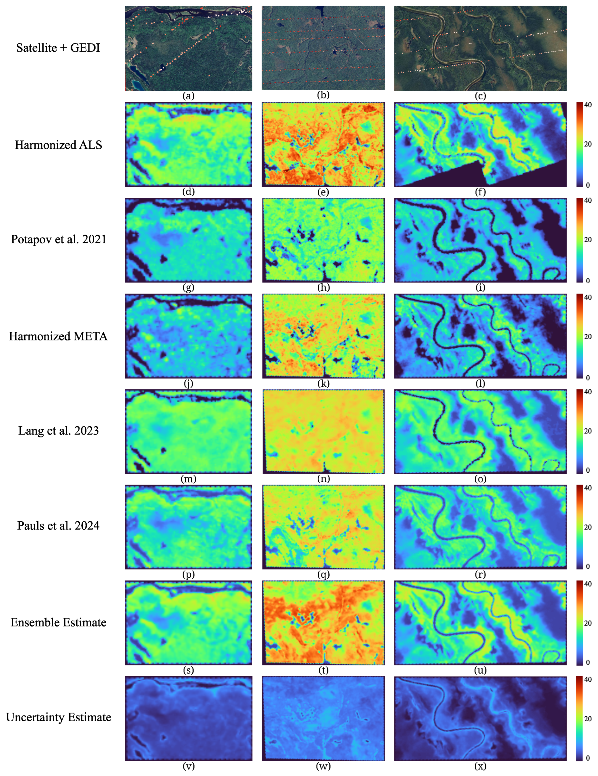
Figure 12 shows canopy-height estimates for three locations representing distinct landscape conditions: a forested area with river corridors (left column), a mature forest with tall canopies and meandering waterways (centre column), and a boreal landscape with meandering rivers, wetlands, and lower-stature forest (right column).
The spatially aggregated ALS reference (panels d–f) provides the validation baseline. In the right column (panel f), the ALS data contains a coverage gap (black triangle), reflecting the limited spatial extent of airborne LiDAR acquisition campaigns—a key motivation for developing wall-to-wall prediction models from satellite data.
The global products exhibit distinct error patterns within the Ontario test domain. Potapov et al. [21] (panels g–i) substantially underestimates height in all three locations, with predominantly dark blue tones where the ALS reference indicates moderate-to-tall canopies, consistent with the limited sensitivity of tree-based ensembles to tall vegetation. Meta [30] (panels j–l) shows the most pronounced underestimation among the four products. In the right (boreal) column, nearly the entire area appears as near-zero height despite clear forest cover in the satellite imagery and non-zero estimates from every other product, suggesting a severe domain-shift effect away from Meta’s training regions. In the centre column, where ALS indicates 25–40 m canopies, Meta compresses the predicted range and underestimates substantially; the left column shows moderate underestimation. Lang et al. [27] (panels m–o) compresses the height range in the opposite direction: in the centre column it predicts moderate-to-tall heights uniformly across areas where ALS reveals substantial local variation, and in the left column it overestimates low-stature areas while underestimating tall canopies. Pauls et al. [28] (panels p–r) reproduces the closest spatial patterns of the four products, particularly along forest–river transitions in the left column, though it still underestimates the tallest canopies in the centre column.
Our ensemble estimate (panels s–u) closely matches the ALS reference across all three locations. The model captures fine-scale structural variability, including canopy-height gradients along river corridors (left column), patches of very tall canopy exceeding 30 m in mature forest (centre column), and the transitions between forested areas and wetlands along the river system (right column). In the right column, our model provides continuous predictions where the ALS reference has a coverage gap, illustrating the operational value of satellite-based wall-to-wall mapping. Water bodies are correctly mapped as zero or near-zero height in all locations. However, slight overestimation is visible in sparsely vegetated areas, consistent with the 0–5 m bin bias discussed in Section 3.7.
The calibrated uncertainty maps (panels v–x) reveal spatially coherent patterns. Uncertainty is lowest (dark blue, <2 m) within homogeneous forest interiors and over water bodies. Moderately elevated values appear along forest edges, river corridors, and land cover transitions. Within the tall-canopy centre column the homogeneous forest interior shows lower uncertainty than its edges and transitions, indicating that—beyond a gradual increase with canopy height—structural heterogeneity and mixed pixels act as an independent source of elevated uncertainty.
At the province scale, Figure S6 (Supplementary Materials) presents the wall-to-wall canopy-height and calibrated uncertainty maps produced by the primary model (W–S–F, LS–S1–AP–X). The canopy-height map reveals clear spatial gradients: taller canopies (20–35 m, green to yellow) dominate the southern Great Lakes–St. Lawrence forest region, while the northern boreal zone exhibits more moderate heights (10–20 m, blue to cyan). Agricultural areas in southern Ontario and urban centres appear as low-height zones. The calibrated uncertainty map shows predominantly low values (1–3 m) across forested areas, with slightly elevated uncertainty along forest–agriculture transitions, near the Hudson Bay Lowlands, and in areas of sparse GEDI coverage. These province-wide patterns are consistent with the local-scale observations from Figure 12 and the quantitative results presented in earlier sections.

3.10. Performance Across Forest Types

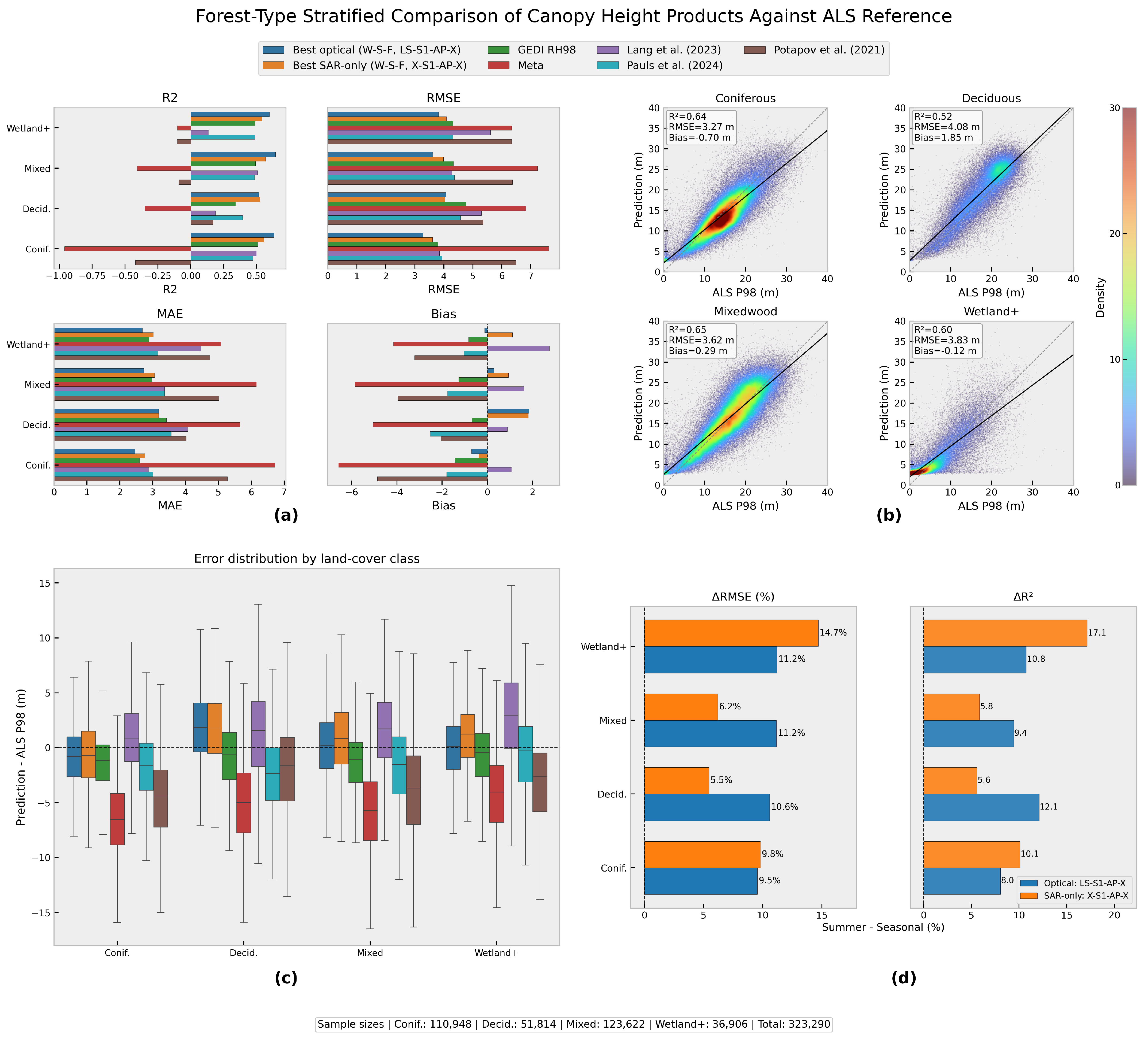
We stratified the GEDI ∩ ALS validation samples by the 2020 North American Land Cover map (NALCMS, 30 m) [38] into four classes: coniferous ( N = 110,948 ), deciduous ( N = 51,814 ), mixedwood ( N = 123,622 ), and treed-wetland ( N = 36,906 ). Figure 13a shows that the primary model (W–S–F LS–S1–AP–X) attains the highest R 2 and lowest RMSE in every forest type, followed by the seasonal SAR-only model (W–S–F X–S1–AP–X). Within the Ontario test domain, the SAR-only model itself outperforms all four global products in every forest class. Among the four global products, Meta shows negative R 2 in most classes, while Potapov et al. [21] shows the strongest negative bias across all classes. Across the four forest types, mixedwood yields the highest R 2 (0.65) and deciduous the lowest (0.52); deciduous also exhibits the largest positive bias (1.85 m) for the primary model.
The density scatter plots in Figure 13b reveal forest-type-specific error patterns for the primary model. Coniferous forests ( R 2 = 0.64 , RMSE = 3.27 m, bias = −0.70 m) show a tight prediction core with a slight negative bias, indicating minor underestimation of tall boreal canopy. Deciduous forests ( R 2 = 0.52 , RMSE = 4.08 m, bias = 1.85 m) show the widest scatter and the most pronounced low-height overestimation cluster above the 1:1 line, suggesting that the GEDI label noise discussed in Section 3.7 is most severe in deciduous stands. Mixedwood forests ( R 2 = 0.65 , RMSE = 3.62 m, bias = 0.29 m) achieve the best overall balance with near-zero bias. Treed-wetland areas ( R 2 = 0.60 , RMSE = 3.83 m, bias = 0.12 m) show a distinct concentration of samples at low ALS values with a secondary cluster at moderate heights, consistent with the heterogeneous vegetation structure of treed wetlands.
The boxplots in Figure 13c confirm that deciduous forests exhibit the widest error dispersion and most positive median error across all products, while coniferous and mixedwood forests show tighter, near-zero-centred distributions for the trained models. The global products display pronounced negative median errors and wide interquartile ranges in every forest type, with Meta and Potapov et al. [21] showing the most extreme negative outliers.
Figure 13d quantifies the seasonal gain (summer-only → seasonal) stratified by forest type for both optical and SAR-only configurations, revealing sensor-specific patterns. The optical model (LS–S1–AP–X) benefits most from seasonal data in deciduous ( Δ RMSE = 10.6%, Δ R 2 = 12.1 % ) and mixedwood ( Δ RMSE = 11.2%, Δ R 2 = 9.4 % ) forests, whereas coniferous forests show more balanced gains between the optical ( Δ RMSE = 9.5%) and SAR ( Δ RMSE = 9.8%) models. The SAR-only model (X–S1–AP–X) achieves its largest seasonal improvement in treed-wetland areas ( Δ RMSE = 14.7%, Δ R 2 = 17.1 % ) and comparatively smaller gains in deciduous (5.5%) and mixedwood (6.2%) forests.

4. Discussion

This study set out to produce spatially continuous 30 m canopy-height estimates, with calibrated pixel-level uncertainty, over Ontario’s managed forest zone by combining seasonal Landsat optical, seasonal Sentinel-1 C-band SAR, and yearly ALOS-PALSAR-2 L-band SAR composites with sparse GEDI training labels in a probabilistic ResUNet ensemble. Validated against an independent airborne-LiDAR archive, the primary model reached R 2 = 0.70 , RMSE = 3.65 m, and near-zero bias (0.23 m), outperforming GEDI itself as a continuous product and surpassing four global canopy-height products across every forest type within the test domain. The experiments support three main conclusions: the outlier-robust Laplace likelihood was the most consequential modelling decision; seasonal compositing and multi-sensor fusion contributed the next-largest, forest-type-dependent gains, including the viability of SAR-only models in cloud-prone regions; and the ensemble produces calibrated uncertainty maps that reflect local structural heterogeneity independent of canopy magnitude.

4.1. Effect of the Laplace NLL Loss

The Gaussian baseline and the Laplace model were trained under identical conditions in every respect except the likelihood: the same ResUNet architecture, the same W–S–F LS–S1–AP–LL input set, the same optimiser and schedule, and the same KDE-based inverse-density sample weighting ( p = 0.8 ). The bias reduction (1.43 m to 0.14 m) is therefore attributable to the Laplace likelihood and not to the sample weighting, which was held constant across both models. The density weighting plays a complementary role: removing it lowers aggregate error but reintroduces tall-canopy underestimation, a known imbalanced-regression trade-off in which minimising overall error favours the densely sampled mid-range while density-based reweighting recovers the rare, high-value targets at some cost to aggregate error [53,54,74,75]. The near-zero bias of the primary model therefore requires both the Laplace likelihood and the weighting. The GEDI labels are strongly heavy-tailed relative to the ALS reference, which is precisely the regime the Laplace likelihood is designed for: the residuals of GEDI RH98 about its conditional mean given ALS P98 have an excess kurtosis of 9.7 (versus 0 for a Gaussian and 3 for a Laplace), with 6.2% of shots falling beyond 2 σ and 1.6% beyond 3 σ of that conditional mean, against Gaussian expectations of 4.6% and 0.3%. This leptokurtic, outlier-heavy label distribution is why substituting the heavier-tailed Laplace likelihood—which down-weights extreme labels rather than letting them drag the conditional mean—reduces the systematic bias so markedly. Because this heavy-tailed noise is a property of the GEDI labels themselves—which supervise every input configuration examined here—the benefit of the Laplace likelihood is not specific to the reference input set, and a factorial ablation confirms that its RMSE advantage over the Gaussian persists both with and without the density weighting (Supplementary Figure S3). The Laplace NLL loss had the largest single effect of any modelling choice tested in this study. Because biases compound when pixel-level predictions are aggregated for carbon-stock accounting [37], the order-of-magnitude bias reduction over the Gaussian baseline is operationally consequential even when accuracy gains in R 2 or RMSE are modest. While Pauls et al. [28] addressed GEDI geolocation noise through a shift-tolerant loss on Sentinel-1/2 composites at global scale, and Fayad et al. [25] introduced a discrete/continuous weighted loss to improve sensitivity to tall trees, neither study reports an ensemble-based pixel-level uncertainty product, and neither used seasonal phenological features. Within the broader probabilistic-CNN family, Lang et al. [26,27] adopted Gaussian NLL with ensembles for canopy-height mapping; the Laplace substitution evaluated here is therefore the next logical step rather than a fundamentally new framework, but the magnitude of the bias reduction supports adopting it as a default for GEDI-supervised training.

4.2. Seasonal Information and Sensor Complementarity

Seasonal compositing produced the second-largest effect after the loss-function change. The primary model’s MAE (2.73 m) and near-zero bias (0.23 m), combined with a regression slope of 0.88, indicate that predictions track ALS P98 proportionally across the full retained height range, without the upper-tail compression typical of tree-ensemble models. Four mechanisms plausibly contribute to the seasonal effect. First, both optical and C-band SAR saturate during peak greenness; phenological signatures—differential green-up timing, senescence, evergreen versus deciduous behaviour—help disambiguate spectral and backscatter signals at saturation [76,77]. Second, multi-season acquisitions vary sun-sensor geometry, capturing structural anisotropy. Third, phenology is correlated with canopy height and forest maturity, providing temporal predictors that DL models can learn alongside spatial features. Fourth, seasonal medians mitigate noise from transient conditions (clouds, haze, drought stress) that disproportionately affect single-season composites. Sentinel-1 emerged as the single most influential sensor: dropping it degrades performance more than dropping ALOS-PALSAR-2 or coordinates. ALOS-PALSAR-2 still contributes meaningfully when combined with Sentinel-1, and the seasonal SAR-fusion model (W–S–F X–S1–AP–X) outperforms the summer optical+SAR model with the same Landsat absent.

4.3. SAR-Only Viability in Cloud-Prone Regions

SAR-only configurations (X–S1–AP–X and X–S1–AP–LL), which exclude optical inputs entirely, outperform all four evaluated global products within the Ontario test domain. The result demonstrates that, in a cloud-prone region with sparse optical coverage, a regionally trained SAR-only model can recover most of the accuracy of an optical+SAR model and substantially exceed the accuracy delivered by global products. Both C-band (Sentinel-1) and L-band (ALOS-PALSAR-2) backscatter saturate at high biomass and canopy height, where additional vertical structure no longer increases the returned signal [35,36]. Three aspects of the framework account for the sensitivity the SAR-only models retain in tall, dense stands. First, the ResUNet does not regress height from a single per-pixel backscatter value: its multi-level encoder–decoder aggregates information over a ∼1.9 km receptive field, so the network uses the spatial texture and context of the backscatter field—edge gradients, patch size, and neighbourhood heterogeneity—rather than backscatter magnitude alone. These contextual cues remain informative where the point-wise signal has saturated. Second, combining C- and L-band provides complementary penetration depths (canopy-top versus branch/trunk scattering), so the two frequencies saturate at different structural levels. Third, seasonal compositing introduces temporal contrast (freeze–thaw, moisture, and phenological modulation of backscatter) beyond the growing-season amplitude, consistent with the seasonal SAR-fusion model (W–S–F X–S1–AP–X) outperforming summer-only SAR. The yearly ALOS-PALSAR-2 mosaic, by contrast, assembles per-pixel best observations from different acquisition dates and thus blends rather than resolves this seasonal signal, consistent with its lower accuracy (X–X–AP–X; RMSE = 4.30 m) than the seasonal SAR-fusion model. A residual underestimation above ∼25 m persists in the SAR-only configurations (Figure 10B), indicating that spatial context attenuates but does not eliminate the saturation limit. The recently launched ALOS-4 [78] (L-band, July 2024), NISAR [79] (L- and S-band, July 2025), and BIOMASS [80] (P-band, April 2025) missions are now in early operational phases; as seasonal multi-frequency SAR composites become routinely available, the L- and P-band contribution can be evaluated in greater depth, particularly in tropical and boreal regions where optical data is unreliable.

4.4. Forest-Type-Specific Behaviour

The forest-type stratified analysis (Figure 13) clarifies how seasonal information interacts with canopy composition. Optical models gain most where leaf-on/leaf-off transitions produce strong inter-seasonal spectral contrast (deciduous and mixedwood forests) [76], whereas coniferous forests with year-round stable optical signatures show smaller, more balanced gains across sensors. The SAR-only model’s largest seasonal gain occurs in treed-wetland areas, where seasonal water-table fluctuations and freeze-thaw cycles strongly modulate C-band backscatter in waterlogged substrates [81]. The positive bias in deciduous forests is consistent with the greater structural complexity of hardwood stands—multi-layered canopies with dense understory broaden GEDI waveforms and can inflate RH98—and with the concentration of deciduous forest in southern Ontario’s more topographically variable Great Lakes–St. Lawrence region, where GEDI ground detection is harder [82].
This positive bias is consistent with the GEDI–ALS comparison of Figure 6a, where GEDI’s regression slope of 0.89 and aggregate bias of −1.11 m indicate net underestimation of ALS P98, once the height distribution is considered. The negative aggregate GEDI bias is driven by the upper tail: a slope below unity means the GEDI–ALS gap grows with canopy height, so the mean is pulled in a negative direction by the few very tall shots, while GEDI overestimates in the dense cluster of low-to-moderate canopies (the near-origin overestimation in Figure 6a, Section 3.7). Deciduous stands in the validation pool are concentrated in this low-to-moderate height range, where dense understory and leaf-on waveform broadening inflate RH98. The forest-type bias is therefore a stratum-specific average over the regime where GEDI overestimates; a model trained on these labels inherits that overestimation, so the deciduous bias is positive (1.85 m), while the all-height GEDI–ALS bias is negative.

4.5. Geographic Coordinates as Inputs

Including latitude/longitude coordinates did not improve performance in this study, in contrast to continental- and global-scale work, where they capture useful climate and continentality gradients [19,27,83]. Within a single province, explicit coordinates risk inducing spatial-autocorrelation bias [84,85], and the CNN’s receptive field already encodes local spatial context implicitly. We therefore selected the coordinate-free configuration as the primary model.

4.6. Performance of Global Products

The relative ranking of the four products in our Ontario test domain (Pauls et al. > Lang et al. ≫ Potapov et al. ≈ Meta; Table 4) is itself informative. The two probabilistic deep learning products that explicitly model GEDI label noise (Pauls et al., Lang et al.) rank above the tree-ensemble (Potapov et al.) and commercial-imagery (Meta) products, though none matches the accuracy of a regionally trained model on this evaluation domain. Meta’s strong negative bias is consistent with Feng et al. [86]’s independent finding of a negative correlation using airborne LiDAR over old-growth tropical forest in Borneo, suggesting the product degrades substantially outside its core training domain. The underestimation by Potapov et al. [21] reflects the regression-to-the-mean tendency of tree-ensemble algorithms [87,88,89]. The directional bias of Lang et al. [27] (overestimating short canopies, underestimating tall ones) is consistent with their reweighting strategy, which discretised the height distribution into 1 m bins with square-root softening and applied the weights only during fine-tuning of the final regression layer; in contrast, the present study uses a continuous KDE-based power-inverse weighting ( p = 0.8 ) applied throughout training across all parameters, which targets the same imbalance more aggressively.

4.7. Low-Canopy Bias and the Role of Anchor Samples

All trained models, including the primary one, exhibit a residual overestimation in the 0–5 m range. This bias is present in the GEDI training labels themselves (Figure 6a) and propagates through the model, indicating it is inherited from the supervision rather than introduced by the network. GEDI is known to overestimate height over sparse vegetation [90,91], particularly on steep slopes, owing to increased ground-return contribution and to terrain-height estimation errors [82,92,93]. The FAO/IPCC operational definition of forest [94,95] requires trees taller than 5 m, so vegetation below this height falls outside the primary scope of forest mapping; nonetheless, the bias degrades carbon-stock estimates derived from these products. A practical mitigation is to inject zero-height anchor samples from auxiliary land-cover sources—pixels confidently identified as water, bare soil, or non-vegetated surface via NDWI [96], MNDWI [97], or NDVI, or via the ESA WorldCover [98] or Ontario Provincial Land Cover map—into the training set with a target of zero. This addresses the training-distribution imbalance at the low end without changes to the architecture, and is a logical complement to the Laplace loss’s outlier robustness.
To avoid conflicting targets in transitional areas (sparse forest, regenerating clearcuts, or wetland margins), anchors would be restricted to pixels with high cross-source agreement and injected only where GEDI observations are absent, so the two label sources are mutually exclusive by construction. They would enter the masked NLL as a finite, down-weighted term rather than a hard zero constraint, allowing the Laplace likelihood to treat a mislabelled anchor as an outlier. We leave the implementation and evaluation of this scheme to future work.

4.8. Uncertainty Maps as a Usable Confidence Layer

Most published canopy-height products do not provide pixel-level uncertainty [20,21,28,31], yet downstream applications such as carbon-stock accounting and forest planning require it. The ensemble approach here, like Lang et al. [26,27], captures aleatoric and epistemic components through a mixture of distributions; substituting Laplace for Gaussian extends that approach to noisy-label regimes. The calibrated uncertainty is monotonically related to observed error (RMSE rises from 2.73 m in Q1 to 4.67 m in Q4) and, although it increases with canopy height, it also reflects local structural heterogeneity independent of canopy magnitude (partial Spearman ρ = 0.48 ), as confirmed by the spatial pattern in Figure 12, where edges and fragmented landscapes show elevated uncertainty relative to homogeneous interiors of comparable canopy height. Together these properties support using the uncertainty layer to filter low-confidence pixels in downstream products, a use that has been suggested but not consistently provided in prior canopy-height work [27].

4.9. Limitations

The evaluation relies on a single fixed five-fold spatial partition. Reusing it across every configuration maximises the internal comparability of the ablation, but does not establish that the absolute metrics or the relative configuration ranking are invariant to the particular fold assignment, nor that the chosen tile size is optimal. Because each configuration is a five-member ensemble and each alternative partitioning scheme would require retraining every member, full re-evaluation under multiple partitions and tile sizes was computationally prohibitive; this applies in particular to ecologically informed designs, such as spatially or environmentally (ecologically) blocked folds [67,99], which would multiply the training cost by the number of blocking schemes tested. Multi-partition and tile-size sensitivity analyses are therefore left for future work.

5. Conclusions

We presented a probabilistic deep learning framework for canopy-height mapping over Ontario that integrates seasonal Landsat, seasonal Sentinel-1, and yearly ALOS-PALSAR-2 composites with sparse GEDI training labels, producing 30 m canopy-height and calibrated pixel-level uncertainty maps. Four findings emerge from the experiments.
First, replacing Gaussian NLL with Laplace NLL—under matched architecture and inputs—improved R 2 by 18.6%, reduced RMSE by 13.7%, and reduced systematic bias by an order of magnitude (1.43 m to 0.14 m), confirming the importance of an outlier-robust likelihood when noisy GEDI samples are the training target.
Second, seasonal multi-temporal compositing outperformed summer-only inputs under matched sensors: R 2 increased by 12.9%, RMSE decreased by 10.8%, and bias dropped by 0.72 m. The forest-type stratified analysis revealed that the seasonal benefit is both sensor- and class-dependent: optical models gained most in deciduous ( Δ RMSE = 10.6%) and mixedwood ( Δ RMSE = 11.2%) forests, while SAR-only models gained most in treed-wetlands ( Δ RMSE = 14.7%).
Third, multi-sensor fusion was the dominant lever on overall accuracy. The primary configuration (W–S–F LS–S1–AP–X) reached R 2 = 0.70 , RMSE = 3.65 m, MAE = 2.73 m, and bias = 0.23 m against the ALS P98 reference. Within the Ontario test domain, even SAR-only configurations outperformed the four evaluated global canopy-height products in every forest class, an operationally meaningful result for cloud-prone regions where optical observations are unreliable.
Fourth, the ensemble-based uncertainty layer—combining aleatoric and epistemic components through a mixture of Laplace distributions with affine post hoc calibration—produces spatially coherent confidence estimates that are monotonically related to observed error and reflect local structural heterogeneity independent of canopy magnitude. This makes them usable as a filtering layer for downstream carbon-stock and forest-management products.
The framework is region-agnostic in inputs but its current evaluation is confined to Ontario’s managed-forest zone. Priority extensions include the integration of seasonal L- and P-band data from ALOS-4, NISAR, and BIOMASS to replace the temporally aggregated ALOS-PALSAR-2 mosaic, GEDI–ICESat-2 fusion to increase training-label density at high latitudes, zero-height anchor injection from auxiliary land-cover maps to correct the residual 0–5 m overestimation, head-to-head comparisons with regionally retrained tree-ensemble baselines, and explicit cross-region validation across Canadian biomes. Given the deep learning core of the framework, applying explainable-AI techniques (e.g., feature-attribution and saliency analyses) to quantify how each sensor, season, and spatial-context cue drives the height and uncertainty predictions is a further promising direction that would increase the interpretability and operational trust of the resulting products.

Supplementary Materials

The following supporting information can be downloaded at: https://www.mdpi.com/article/10.3390/rs18152477/s1. Figure S1: Study-area characterisation in geographic coordinates (forest-class distribution and study-tile roles); Figure S2: Comparison of the multi-sensor model inputs and the ALS height reference over three representative regions; Figure S3: Loss × weighting ablation (Gaussian versus Laplace NLL, each with and without KDE inverse-density weighting); Figure S4: Scatter plots of the optical-containing ablation configurations not shown in the main text; Figure S5: Scatter plots of the SAR-only experiments against the ALS P98 reference; Figure S6: Province-wide canopy-height and calibrated-uncertainty prediction maps.

Author Contributions

Conceptualisation, J.B.; methodology, J.B.; software, J.B. and C.R.; validation, J.B.; formal analysis, J.B., C.R., C.S., and A.G.; investigation, J.B.; writing—original draft preparation, J.B.; writing—review and editing, C.R., C.S., D.C., and A.G.; visualisation, J.B. and C.R.; supervision, A.G.; project administration, A.G.; funding acquisition, A.G. All authors have read and agreed to the published version of the manuscript.

Funding

This research was funded by the Natural Sciences and Engineering Research Council of Canada (NSERC), the Sustainable Forestry Initiative program, and the Environment and Climate Change Canada (ECCC) Grants and Contributions program (grant number GCXE24S085). Computational resources were provided by the Digital Research Alliance of Canada and the Google Cloud Research Credits program.

Data Availability Statement

All satellite data used in this study are publicly available. Landsat 7 and 8 surface reflectance (Collection 2, Tier 1), Sentinel-1 SAR Ground Range Detected imagery, and GEDI L2A relative height products were accessed through the Google Earth Engine platform [39]. ALOS-PALSAR-2 yearly mosaic composites were obtained from the Japan Aerospace Exploration Agency (JAXA) Global PALSAR-2/PALSAR Yearly Mosaic via Google Earth Engine. The Forest Resources Inventory (FRI) leaf-on Single Photon LiDAR products—canopy-height model, Digital Surface Model, and Digital Terrain Model—are available from the Ontario GeoHub (https://geohub.lio.gov.on.ca/maps/forest-resources-inventory-leaf-on-lidar, accessed on 15 July 2026) [42]. The 2020 North American Land Cover map (NALCMS, 30 m), used for forest-type stratification, is available from the Commission for Environmental Cooperation (http://www.cec.org/north-american-environmental-atlas/land-cover-30m-2020/, accessed on 15 July 2026) [38]. The four global canopy-height products used as benchmarks were obtained from their respective public repositories: Meta [30], Lang et al. [27], Potapov et al. [21], and Pauls et al. [28]. The Seasonal Image Composite Algorithm (SICA), data preprocessing pipeline, model training scripts, configuration files for every reported experimental configuration, trained ensemble weights, and the final 30 m wall-to-wall canopy-height and calibrated-uncertainty rasters for Ontario are available at https://github.com/MacRemoteSensing/gedi-guided-ch-uncertainty (accessed on 15 July 2026).

Acknowledgments

The findings and views described herein do not necessarily reflect those of Planet Labs PBC.

Conflicts of Interest

Author Camile Sothe was employed by the company Planet Labs PBC. The remaining authors declare that the research was conducted in the absence of any commercial or financial relationships that could be construed as a potential conflict of interest.

Abbreviations

The following abbreviations are used in this manuscript:
AGBAboveground Biomass
ALSAirborne LiDAR
BAPBest Available Pixel
CHCanopy Height
CHMCanopy-Height Model
CNNConvolutional Neural Network
DLDeep Learning
DSMDigital Surface Model
DTMDigital Terrain Model
FCNFully Convolutional Network
FRIForest Resources Inventory
GEDIGlobal Ecosystem Dynamics Investigation
GEEGoogle Earth Engine
ISSInternational Space Station
KDEKernel Density Estimate
LDSLabel Distribution Smoothing
LiDARLight Detection and Ranging
NLLNegative Log-Likelihood
RH98Relative Height 98th percentile
RMSERoot Mean Square Error
SARSynthetic Aperture Radar
SICASeasonal Image Composite Algorithm
SPLSingle Photon LiDAR
UCEUncertainty Calibration Error
UCNNUncertainty Convolutional Neural Network

References

  1. Asner, G.P.; Martin, R.E.; Carranza-Jiménez, L.; Sinca, F.; Tupayachi, R.; Anderson, C.B.; Martinez, P. Functional and biological diversity of foliar spectra in tree canopies throughout the Andes to Amazon region. New Phytol. 2014, 204, 127–139. [Google Scholar] [CrossRef] [Scilit] [PubMed]
  2. Mitchard, E.T.; Feldpausch, T.R.; Brienen, R.J.; Lopez-Gonzalez, G.; Monteagudo, A.; Baker, T.R.; Lewis, S.L.; Lloyd, J.; Quesada, C.A.; Gloor, M.; et al. Markedly divergent estimates of A mazon forest carbon density from ground plots and satellites. Glob. Ecol. Biogeogr. 2014, 23, 935–946. [Google Scholar] [CrossRef] [Scilit] [PubMed]
  3. Stovall, A.E.; Fatoyinbo, T.; Thomas, N.M.; Armston, J.; Ebanega, M.O.; Simard, M.; Trettin, C.; Zogo, R.V.O.; Aken, I.A.; Debina, M.; et al. Comprehensive comparison of airborne and spaceborne SAR and LiDAR estimates of forest structure in the tallest mangrove forest on earth. Sci. Remote Sens. 2021, 4, 100034. [Google Scholar] [CrossRef] [Scilit]
  4. Pan, Y.; Birdsey, R.A.; Phillips, O.L.; Houghton, R.A.; Fang, J.; Kauppi, P.E.; Keith, H.; Kurz, W.A.; Ito, A.; Lewis, S.L.; et al. The enduring world forest carbon sink. Nature 2024, 631, 563–569. [Google Scholar] [CrossRef] [Scilit] [PubMed]
  5. IPCC. Climate Change 2023: Synthesis Report. Contribution of Working Groups I, II and III to the Sixth Assessment Report of the Intergovernmental Panel on Climate Change; IPCC: Geneva, Switzerland, 2023. [Google Scholar] [CrossRef] [Scilit]
  6. Jucker, T.; Caspersen, J.; Chave, J.; Antin, C.; Barbier, N.; Bongers, F.; Dalponte, M.; van Ewijk, K.Y.; Forrester, D.I.; Haeni, M.; et al. Allometric equations for integrating remote sensing imagery into forest monitoring programmes. Glob. Change Biol. 2017, 23, 177–190. [Google Scholar] [CrossRef] [Scilit] [PubMed]
  7. Carreiras, J.M.; Quegan, S.; Le Toan, T.; Minh, D.H.T.; Saatchi, S.S.; Carvalhais, N.; Reichstein, M.; Scipal, K. Coverage of high biomass forests by the ESA BIOMASS mission under defense restrictions. Remote Sens. Environ. 2017, 196, 154–162. [Google Scholar] [CrossRef] [Scilit]
  8. Csillik, O.; Kumar, P.; Mascaro, J.; O’Shea, T.; Asner, G.P. Monitoring tropical forest carbon stocks and emissions using Planet satellite data. Sci. Rep. 2019, 9, 17831. [Google Scholar] [CrossRef] [Scilit] [PubMed]
  9. Qi, W.; Saarela, S.; Armston, J.; Ståhl, G.; Dubayah, R. Forest biomass estimation over three distinct forest types using TanDEM-X InSAR data and simulated GEDI lidar data. Remote Sens. Environ. 2019, 232, 111283. [Google Scholar] [CrossRef] [Scilit]
  10. Hentz, Â.M.; Silva, C.A.; Dalla Corte, A.P.; Netto, S.P.; Strager, M.P.; Klauberg, C. Estimating forest uniformity in Eucalyptus spp. and Pinus taeda L. stands using field measurements and structure from motion point clouds generated from unmanned aerial vehicle (UAV) data collection. For. Syst. 2018, 27, e005. [Google Scholar] [CrossRef] [Scilit]
  11. Silva, C.; Hudak, A.; Vierling, L.; Valbuena, R.; Cardil, A.; Mohan, M.; Almeida, D.; Broadbent, E.; Zambrano, A.; Wilkinson, B.; et al. Treetop: A Shiny-Based Application for Extracting Forest Information from LiDAR Data. Version 0.0. 3. Methods Ecol. Evol. 2022, 13, 1164–1176. [Google Scholar] [CrossRef] [Scilit]
  12. Stephenson, N.L.; Das, A.; Condit, R.; Russo, S.; Baker, P.; Beckman, N.G.; Coomes, D.; Lines, E.; Morris, W.; Rüger, N.; et al. Rate of tree carbon accumulation increases continuously with tree size. Nature 2014, 507, 90–93. [Google Scholar] [CrossRef] [Scilit] [PubMed]
  13. Wulder, M.A.; White, J.C.; Nelson, R.F.; Næsset, E.; Ørka, H.O.; Coops, N.C.; Hilker, T.; Bater, C.W.; Gobakken, T. Lidar sampling for large-area forest characterization: A review. Remote Sens. Environ. 2012, 121, 196–209. [Google Scholar] [CrossRef] [Scilit]
  14. Tompalski, P.; Coops, N.C.; White, J.C.; Goodbody, T.R.; Hennigar, C.R.; Wulder, M.A.; Socha, J.; Woods, M.E. Estimating changes in forest attributes and enhancing growth projections: A review of existing approaches and future directions using airborne 3D point cloud data. Curr. For. Rep. 2021, 7, 1–24. [Google Scholar] [CrossRef] [Scilit]
  15. Dubayah, R.; Blair, J.B.; Goetz, S.; Fatoyinbo, L.; Hansen, M.; Healey, S.; Hofton, M.; Hurtt, G.; Kellner, J.; Luthcke, S.; et al. The Global Ecosystem Dynamics Investigation: High-resolution laser ranging of the Earth’s forests and topography. Sci. Remote Sens. 2020, 1, 100002. [Google Scholar] [CrossRef] [Scilit]
  16. Liu, A.; Cheng, X.; Chen, Z. Performance evaluation of GEDI and ICESat-2 laser altimeter data for terrain and canopy height retrievals. Remote Sens. Environ. 2021, 264, 112571. [Google Scholar] [CrossRef] [Scilit]
  17. Qi, W.; Armston, J.; Choi, C.; Stovall, A.; Saarela, S.; Pardini, M.; Fatoyinbo, L.; Papathanassiou, K.; Pascual, A.; Dubayah, R. Mapping large-scale pantropical forest canopy height by integrating GEDI lidar and TanDEM-X InSAR data. Remote Sens. Environ. 2025, 318, 114534. [Google Scholar] [CrossRef] [Scilit]
  18. Krieger, G.; Moreira, A.; Fiedler, H.; Hajnsek, I.; Werner, M.; Younis, M.; Zink, M. TanDEM-X: A satellite formation for high-resolution SAR interferometry. IEEE Trans. Geosci. Remote Sens. 2007, 45, 3317–3341. [Google Scholar] [CrossRef] [Scilit]
  19. Silveira, E.M.; Radeloff, V.C.; Martinuzzi, S.; Pastur, G.J.M.; Bono, J.; Politi, N.; Lizarraga, L.; Rivera, L.O.; Ciuffoli, L.; Rosas, Y.M.; et al. Nationwide native forest structure maps for Argentina based on forest inventory data, SAR Sentinel-1 and vegetation metrics from Sentinel-2 imagery. Remote Sens. Environ. 2023, 285, 113391. [Google Scholar] [CrossRef] [Scilit]
  20. Sothe, C.; Gonsamo, A.; Lourenço, R.B.; Kurz, W.A.; Snider, J. Spatially continuous mapping of forest canopy height in Canada by combining GEDI and ICESat-2 with PALSAR and Sentinel. Remote Sens. 2022, 14, 5158. [Google Scholar] [CrossRef] [Scilit]
  21. Potapov, P.; Li, X.; Hernandez-Serna, A.; Tyukavina, A.; Hansen, M.C.; Kommareddy, A.; Pickens, A.; Turubanova, S.; Tang, H.; Silva, C.E.; et al. Mapping global forest canopy height through integration of GEDI and Landsat data. Remote Sens. Environ. 2021, 253, 112165. [Google Scholar] [CrossRef] [Scilit]
  22. Travers-Smith, H.; Coops, N.C.; Mulverhill, C.; Wulder, M.A.; Ignace, D.; Lantz, T.C. Mapping vegetation height and identifying the northern forest limit across Canada using ICESat-2, Landsat time series and topographic data. Remote Sens. Environ. 2024, 305, 114097. [Google Scholar] [CrossRef] [Scilit]
  23. Wright, M.N.; Dankowski, T.; Ziegler, A. Unbiased split variable selection for random survival forests using maximally selected rank statistics. Stat. Med. 2017, 36, 1272–1284. [Google Scholar] [CrossRef] [Scilit] [PubMed]
  24. Hengl, T.; Nussbaum, M.; Wright, M.N.; Heuvelink, G.B.; Gräler, B. Random forest as a generic framework for predictive modeling of spatial and spatio-temporal variables. PeerJ 2018, 6, e5518. [Google Scholar] [CrossRef] [Scilit] [PubMed]
  25. Fayad, I.; Ciais, P.; Schwartz, M.; Wigneron, J.P.; Baghdadi, N.; de Truchis, A.; d’Aspremont, A.; Frappart, F.; Saatchi, S.; Sean, E.; et al. Hy-TeC: A hybrid vision transformer model for high-resolution and large-scale mapping of canopy height. Remote Sens. Environ. 2024, 302, 113945. [Google Scholar] [CrossRef] [Scilit]
  26. Lang, N.; Kalischek, N.; Armston, J.; Schindler, K.; Dubayah, R.; Wegner, J.D. Global canopy height regression and uncertainty estimation from GEDI LIDAR waveforms with deep ensembles. Remote Sens. Environ. 2022, 268, 112760. [Google Scholar] [CrossRef] [Scilit]
  27. Lang, N.; Jetz, W.; Schindler, K.; Wegner, J.D. A high-resolution canopy height model of the Earth. Nat. Ecol. Evol. 2023, 7, 1778–1789. [Google Scholar] [CrossRef] [Scilit] [PubMed]
  28. Pauls, J.; Zimmer, M.; Kelly, U.M.; Schwartz, M.; Saatchi, S.; Ciais, P.; Pokutta, S.; Brandt, M.; Gieseke, F. Estimating canopy height at scale. arXiv 2024, arXiv:2406.01076. [Google Scholar]
  29. Liu, J.; Quan, Y.; Wang, B.; Shi, J.; Ming, L.; Li, M. Estimation of Forest Stock Volume Combining Airborne LiDAR Sampling Approaches with Multi-Sensor Imagery. Forests 2023, 14, 2453. [Google Scholar] [CrossRef] [Scilit]
  30. Tolan, J.; Yang, H.I.; Nosarzewski, B.; Couairon, G.; Vo, H.V.; Brandt, J.; Spore, J.; Majumdar, S.; Haziza, D.; Vamaraju, J.; et al. Very high resolution canopy height maps from RGB imagery using self-supervised vision transformer and convolutional decoder trained on aerial lidar. Remote Sens. Environ. 2024, 300, 113888. [Google Scholar] [CrossRef] [Scilit]
  31. Wagner, F.H.; Roberts, S.; Ritz, A.L.; Carter, G.; Dalagnol, R.; Favrichon, S.; Hirye, M.C.M.; Brandt, M.; Ciais, P.; Saatchi, S. Sub-meter tree height mapping of California using aerial images and LiDAR-informed U-Net model. Remote Sens. Environ. 2024, 305, 114099. [Google Scholar] [CrossRef] [Scilit]
  32. Barbier, N.; Couteron, P.; Proisy, C.; Malhi, Y.; Gastellu-Etchegorry, J.P. The variation of apparent crown size and canopy heterogeneity across lowland Amazonian forests. Glob. Ecol. Biogeogr. 2010, 19, 72–84. [Google Scholar] [CrossRef] [Scilit]
  33. Couteron, P.; Pelissier, R.; Nicolini, E.A.; Paget, D. Predicting tropical forest stand structure parameters from Fourier transform of very high-resolution remotely sensed canopy images. J. Appl. Ecol. 2005, 42, 1121–1128. [Google Scholar] [CrossRef] [Scilit]
  34. Ploton, P.; Pélissier, R.; Barbier, N.; Proisy, C.; Ramesh, B.R.; Couteron, P. Canopy texture analysis for large-scale assessments of tropical forest stand structure and biomass. In Treetops at Risk: Challenges of Global Canopy Ecology and Conservation; Lowman, M.D., Devy, S., Ganesh, T., Eds.; Springer: New York, NY, USA, 2013; pp. 237–245. [Google Scholar] [CrossRef] [Scilit]
  35. Lu, D.; Chen, Q.; Wang, G.; Moran, E.; Batistella, M.; Zhang, M.; Vaglio Laurin, G.; Saah, D. Aboveground forest biomass estimation with Landsat and LiDAR data and uncertainty analysis of the estimates. Int. J. For. Res. 2012, 2012, 436537. [Google Scholar] [CrossRef] [Scilit]
  36. Le Toan, T.; Quegan, S.; Davidson, M.; Balzter, H.; Paillou, P.; Papathanassiou, K.; Plummer, S.; Rocca, F.; Saatchi, S.; Shugart, H.; et al. The BIOMASS mission: Mapping global forest biomass to better understand the terrestrial carbon cycle. Remote Sens. Environ. 2011, 115, 2850–2860. [Google Scholar] [CrossRef] [Scilit]
  37. Duncanson, L.; Kellner, J.R.; Armston, J.; Dubayah, R.; Minor, D.M.; Hancock, S.; Healey, S.P.; Patterson, P.L.; Saarela, S.; Marselis, S.; et al. Aboveground biomass density models for NASA’s Global Ecosystem Dynamics Investigation (GEDI) lidar mission. Remote Sens. Environ. 2022, 270, 112845. [Google Scholar] [CrossRef] [Scilit]
  38. Commission for Environmental Cooperation (CEC). 2020 Land Cover of North America at 30 Meters; Ed. 1.0, Raster Digital Data [30 m]; North American Land Change Monitoring System (NALCMS): Montreal, QC, Canada; Canada Centre for Remote Sensing (CCRS): Ottawa, ON, Canada; U.S. Geological Survey (USGS): Reston, VA, USA; CONABIO: Mexico City, Mexico; CONAFOR: Zapopan, Mexico; INEGI: Aguascalientes, Mexico, 2023; Available online: http://www.cec.org/north-american-environmental-atlas/land-cover-30m-2020/ (accessed on 15 July 2026).
  39. Gorelick, N.; Hancher, M.; Dixon, M.; Ilyushchenko, S.; Thau, D.; Moore, R. Google Earth Engine: Planetary-scale geospatial analysis for everyone. Remote Sens. Environ. 2017, 202, 18–27. [Google Scholar] [CrossRef] [Scilit]
  40. Thompson, S.D.; Nelson, T.A.; White, J.C.; Wulder, M.A. Mapping dominant tree species over large forested areas using Landsat best-available-pixel image composites. Can. J. Remote Sens. 2015, 41, 203–218. [Google Scholar] [CrossRef] [Scilit]
  41. Mao, L.; Bater, C.W.; Stadt, J.J.; White, B.; Tompalski, P.; Coops, N.C.; Nielsen, S.E. Environmental landscape determinants of maximum forest canopy height of boreal forests. J. Plant Ecol. 2019, 12, 96–102. [Google Scholar] [CrossRef] [Scilit]
  42. Bilyk, A.; Pulkki, R.; Shahi, C.; Larocque, G.R. Development of the Ontario Forest Resources Inventory: A historical review. Can. J. For. Res. 2021, 51, 198–209. [Google Scholar] [CrossRef] [Scilit]
  43. Oquab, M.; Darcet, T.; Moutakanni, T.; Vo, H.; Szafraniec, M.; Khalidov, V.; Fernandez, P.; Haziza, D.; Massa, F.; El-Nouby, A.; et al. Dinov2: Learning robust visual features without supervision. arXiv 2023, arXiv:2304.07193. [Google Scholar] [CrossRef] [Scilit]
  44. Kutchartt, G.; Neuenschwander, A.; Hancock, S.; Hofton, M.; Blair, J.; Luthcke, S. Assessment of ranging and positioning accuracy of the GEDI laser altimeter on the International Space Station. Remote Sens. Environ. 2022, 274, 112963. [Google Scholar] [CrossRef] [Scilit]
  45. Long, J.; Shelhamer, E.; Darrell, T. Fully convolutional networks for semantic segmentation. In Proceedings of the IEEE Conference on Computer Vision and Pattern Recognition; IEEE: Piscataway, NJ, USA, 2015; pp. 3431–3440. [Google Scholar] [CrossRef] [Scilit]
  46. Diakogiannis, F.I.; Waldner, F.; Caccetta, P.; Wu, C. ResUNet-a: A deep learning framework for semantic segmentation of remotely sensed data. ISPRS J. Photogramm. Remote Sens. 2020, 162, 94–114. [Google Scholar] [CrossRef] [Scilit]
  47. Lakshminarayanan, B.; Pritzel, A.; Blundell, C. Simple and scalable predictive uncertainty estimation using deep ensembles. In Proceedings of the Advances in Neural Information Processing Systems (NeurIPS), Long Beach, CA, USA, 4–9 December 2017; Volume 30. [Google Scholar]
  48. Chen, L.C.; Papandreou, G.; Kokkinos, I.; Murphy, K.; Yuille, A.L. Deeplab: Semantic image segmentation with deep convolutional nets, atrous convolution, and fully connected crfs. IEEE Trans. Pattern Anal. Mach. Intell. 2017, 40, 834–848. [Google Scholar] [CrossRef] [Scilit] [PubMed]
  49. He, K.; Zhang, X.; Ren, S.; Sun, J. Identity mappings in deep residual networks. In Proceedings of the European Conference on Computer Vision; Springer: Berlin/Heidelberg, Germany, 2016; pp. 630–645. [Google Scholar]
  50. Ioffe, S. Batch normalization: Accelerating deep network training by reducing internal covariate shift. arXiv 2015, arXiv:1502.03167. [Google Scholar]
  51. Nair, D.S.; Hochgeschwender, N.; Olivares-Méndez, M.A. Maximum likelihood uncertainty estimation: Robustness to outliers. arXiv 2022, arXiv:2202.03870. [Google Scholar]
  52. Kotz, S.; Kozubowski, T.; Podgorski, K. The Laplace Distribution and Generalizations: A Revisit with Applications to Communications, Economics, Engineering, and Finance; Springer Science & Business Media: Berlin/Heidelberg, Germany, 2012. [Google Scholar] [CrossRef] [Scilit]
  53. Yang, Y.; Zha, K.; Chen, Y.; Wang, H.; Katabi, D. Delving into deep imbalanced regression. In Proceedings of the International Conference on Machine Learning; PMLR: Cambridge, MA, USA, 2021; pp. 11842–11851. [Google Scholar]
  54. Steininger, M.; Kobs, K.; Davidson, P.; Krause, A.; Hotho, A. Density-based weighting for imbalanced regression. Mach. Learn. 2021, 110, 2187–2211. [Google Scholar] [CrossRef] [Scilit]
  55. Lahssini, K.; Baghdadi, N.; Le Maire, G.; Fayad, I. Influence of GEDI acquisition and processing parameters on canopy height estimates over tropical forests. Remote Sens. 2022, 14, 6264. [Google Scholar] [CrossRef] [Scilit]
  56. Fayad, I.; Baghdadi, N.; Riedi, J. Quality assessment of acquired gedi waveforms: Case study over france, tunisia and french guiana. Remote Sens. 2021, 13, 3144. [Google Scholar] [CrossRef] [Scilit]
  57. Tang, H.; Stoker, J.; Luthcke, S.; Armston, J.; Lee, K.; Blair, B.; Hofton, M. Evaluating and mitigating the impact of systematic geolocation error on canopy height measurement performance of GEDI. Remote Sens. Environ. 2023, 291, 113571. [Google Scholar] [CrossRef] [Scilit]
  58. Laves, M.H.; Ihler, S.; Kortmann, K.P.; Ortmaier, T. Well-calibrated model uncertainty with temperature scaling for dropout variational inference. arXiv 2019, arXiv:1909.13550. [Google Scholar]
  59. Laves, M.H.; Ihler, S.; Fast, J.F.; Kahrs, L.A.; Ortmaier, T. Well-Calibrated Regression Uncertainty in Medical Imaging with Deep Learning. In Proceedings of the Third Conference on Medical Imaging with Deep Learning, Montreal, QC, Canada, 6–8 July 2020; Proceedings of Machine Learning Research; Arbel, T., Ben Ayed, I., de Bruijne, M., Descoteaux, M., Lombaert, H., Pal, C., Eds.; PMLR: Cambridge, MA, USA, 2020; Volume 121, pp. 393–412. [Google Scholar]
  60. Kuleshov, V.; Fenner, N.; Ermon, S. Accurate uncertainties for deep learning using calibrated regression. In Proceedings of the International Conference on Machine Learning; PMLR: Cambridge, MA, USA, 2018; pp. 2796–2804. [Google Scholar]
  61. Dawood, T.; Chen, C.; Sidhu, B.S.; Ruijsink, B.; Gould, J.; Porter, B.; Elliott, M.K.; Mehta, V.; Rinaldi, C.A.; Puyol-Antón, E.; et al. Uncertainty aware training to improve deep learning model calibration for classification of cardiac MR images. Med. Image Anal. 2023, 88, 102861. [Google Scholar] [CrossRef] [Scilit] [PubMed]
  62. Zhang, H.; Zhang, Y.; Yu, Y.; Madeka, D.; Foster, D.; Xing, E.; Lakkaraju, H.; Kakade, S. A Study on the Calibration of In-context Learning. In Proceedings of the 2024 Conference of the North American Chapter of the Association for Computational Linguistics: Human Language Technologies; Duh, K., Gomez, H., Bethard, S., Eds.; Association for Computational Linguistics (ACL): Mexico City, Mexico, 2024; Volume 1: Long Papers, pp. 6118–6136. [Google Scholar] [CrossRef] [Scilit]
  63. Platt, J. Probabilistic outputs for support vector machines and comparisons to regularized likelihood methods. Adv. Large Margin Classif. 1999, 10, 61–74. [Google Scholar]
  64. Réjou-Méchain, M.; Muller-Landau, H.C.; Detto, M.; Thomas, S.C.; Le Toan, T.; Saatchi, S.S.; Barreto-Silva, J.S.; Bourg, N.A.; Bunyavejchewin, S.; Butt, N.; et al. Local spatial structure of forest biomass and its consequences for remote sensing of carbon stocks. Biogeosciences 2014, 11, 6827–6840. [Google Scholar] [CrossRef] [Scilit]
  65. Mascaro, J.; Detto, M.; Asner, G.P.; Muller-Landau, H.C. Evaluating uncertainty in mapping forest carbon with airborne LiDAR. Remote Sens. Environ. 2011, 115, 3770–3774. [Google Scholar] [CrossRef] [Scilit]
  66. Ploton, P.; Mortier, F.; Réjou-Méchain, M.; Barbier, N.; Piber, A.; Rossi, V.; Dormann, C.F.; Cornu, G.; Viennois, G.; Bayol, N.; et al. Spatial validation reveals poor predictive performance of large-scale ecological mapping models. Nat. Commun. 2020, 11, 4540. [Google Scholar] [CrossRef] [Scilit] [PubMed]
  67. Roberts, D.R.; Bahn, V.; Ciuti, S.; Boyce, M.S.; Elith, J.; Guillera-Arroita, G.; Hauenstein, S.; Lahoz-Monfort, J.J.; Schröder, B.; Thuiller, W.; et al. Cross-validation strategies for data with temporal, spatial, hierarchical, or phylogenetic structure. Ecography 2017, 40, 913–929. [Google Scholar] [CrossRef] [Scilit]
  68. Chan, T.F.; Golub, G.H.; LeVeque, R.J. Algorithms for computing the sample variance: Analysis and recommendations. Am. Stat. 1983, 37, 242–247. [Google Scholar] [CrossRef] [Scilit]
  69. Pedregosa, F.; Varoquaux, G.; Gramfort, A.; Michel, V.; Thirion, B.; Grisel, O.; Blondel, M.; Prettenhofer, P.; Weiss, R.; Dubourg, V.; et al. Scikit-learn: Machine learning in Python. J. Mach. Learn. Res. 2011, 12, 2825–2830. [Google Scholar]
  70. Huang, L.; Qin, J.; Zhou, Y.; Zhu, F.; Liu, L.; Shao, L. Normalization techniques in training dnns: Methodology, analysis and application. IEEE Trans. Pattern Anal. Mach. Intell. 2023, 45, 10173–10196. [Google Scholar] [CrossRef] [Scilit] [PubMed]
  71. Abadi, M.; Agarwal, A.; Barham, P.; Brevdo, E.; Chen, Z.; Citro, C.; Corrado, G.S.; Davis, A.; Dean, J.; Devin, M.; et al. TensorFlow: Large-Scale Machine Learning on Heterogeneous Systems. 2015. Available online: https://www.tensorflow.org (accessed on 15 July 2026).
  72. Kingma, D.P.; Ba, J. Adam: A method for stochastic optimization. arXiv 2014, arXiv:1412.6980. [Google Scholar] [CrossRef] [Scilit]
  73. Loshchilov, I.; Hutter, F. Sgdr: Stochastic gradient descent with warm restarts. arXiv 2016, arXiv:1608.03983. [Google Scholar] [CrossRef] [Scilit]
  74. Branco, P.; Torgo, L.; Ribeiro, R.P. A survey of predictive modeling on imbalanced domains. ACM Comput. Surv. 2016, 49, 31. [Google Scholar] [CrossRef] [Scilit]
  75. Ribeiro, R.P.; Moniz, N. Imbalanced regression and extreme value prediction. Mach. Learn. 2020, 109, 1803–1835. [Google Scholar] [CrossRef] [Scilit]
  76. Chen, J.M.; Liu, J.; Leblanc, S.G.; Lacaze, R.; Roujean, J.L. Multi-angular optical remote sensing for assessing vegetation structure and carbon absorption. Remote Sens. Environ. 2003, 84, 516–525. [Google Scholar] [CrossRef] [Scilit]
  77. Yan, X.; Li, J.; Smith, A.R.; Yang, D.; Ma, T.; Su, Y.; Shao, J. Evaluation of machine learning methods and multi-source remote sensing data combinations to construct forest above-ground biomass models. Int. J. Digit. Earth 2023, 16, 4471–4491. [Google Scholar] [CrossRef] [Scilit]
  78. Ohki, M.; Motohka, T.; Kankaku, Y.; Miura, S.H.; Tadono, T.; Arikawa, Y. Advanced Land Observing Satellite-4: Mission Concepts and Technical Overview: Pioneering a new era of L-band SAR. IEEE Geosci. Remote Sens. Mag. 2025, 13, 35–40. [Google Scholar] [CrossRef] [Scilit]
  79. Kellogg, K.; Hoffman, P.; Standley, S.; Shaffer, S.; Rosen, P.; Edelstein, W.; Dunn, C.; Baker, C.; Barela, P.; Shen, Y.; et al. NASA-ISRO synthetic aperture radar (NISAR) mission. In Proceedings of the 2020 IEEE Aerospace Conference; IEEE: Piscataway, NJ, USA, 2020; pp. 1–21. [Google Scholar]
  80. European Space Agency (ESA). Introducing BIOMASS; European Space Agency (ESA): Paris, France, 2023. [Google Scholar]
  81. Sahour, H.; Kemink, K.M.; O’Connell, J. Integrating SAR and Optical Remote Sensing for Conservation-Targeted Wetlands Mapping. Remote Sens. 2022, 14, 159. [Google Scholar] [CrossRef] [Scilit]
  82. Adam, M.; Urbazaev, M.; Dubois, C.; Schmullius, C. Accuracy assessment of GEDI terrain elevation and canopy height estimates in European temperate forests: Influence of environmental and acquisition parameters. Remote Sens. 2020, 12, 3948. [Google Scholar] [CrossRef] [Scilit]
  83. Matasci, G.; Coops, N.C.; Williams, D.A.; Page, N. Mapping tree canopies in urban environments using airborne laser scanning (ALS): A Vancouver case study. For. Ecosyst. 2018, 5, 31. [Google Scholar] [CrossRef] [Scilit]
  84. Min, W.; Chen, Y.; Huang, W.; Wilson, J.P.; Tang, H.; Guo, M.; Xu, R. Incorporating of spatial effects in forest canopy height mapping using airborne, spaceborne lidar and spatial continuous remote sensing data. Int. J. Appl. Earth Obs. Geoinf. 2024, 133, 104123. [Google Scholar] [CrossRef] [Scilit]
  85. Shen, H.; Wang, Y.; Guan, X.; Huang, W.; Chen, J.; Lin, D.; Gan, W. A spatiotemporal constrained machine learning method for OCO-2 solar-induced chlorophyll fluorescence (SIF) reconstruction. IEEE Trans. Geosci. Remote Sens. 2022, 60, 4413817. [Google Scholar] [CrossRef] [Scilit]
  86. Feng, Z.; Jaffer, S.; Knezevic, J.; Sormunen, S.; Young, R.; Lisaius, M.C.; Immitzer, M.; Ball, J.; Atzberger, C.; Coomes, D.A.; et al. TESSERA: Temporal Embeddings of Surface Spectra for Earth Representation and Analysis. In Proceedings of the IEEE/CVF Conference on Computer Vision and Pattern Recognition (CVPR); IEEE: Piscataway, NJ, USA, 2026; pp. 1–11. [Google Scholar]
  87. Friedman, J.H. Greedy function approximation: A gradient boosting machine. Ann. Stat. 2001, 29, 1189–1232. [Google Scholar] [CrossRef] [Scilit]
  88. Meinshausen, N. Quantile Regression Forests. J. Mach. Learn. Res. 2006, 7, 983–999. [Google Scholar]
  89. Pal, M. Random forest classifier for remote sensing classification. Int. J. Remote Sens. 2005, 26, 217–222. [Google Scholar] [CrossRef] [Scilit]
  90. Dhargay, S.; Lyell, C.S.; Brown, T.P.; Inbar, A.; Sheridan, G.J.; Lane, P.N.J. Performance of GEDI space-borne lidar for quantifying structural variation in the temperate forests of south-eastern Australia. Remote Sens. 2022, 14, 3615. [Google Scholar] [CrossRef] [Scilit]
  91. Moudrý, V.; Gdullová, K.; Holešinský, T.; Wild, J.; Kopecký, M.; Lánský, D.; Adámek, M. How to Find Accurate Terrain and Canopy Height GEDI Footprints in Temperate Forests and Grasslands? Earth Space Sci. 2024, 11, e2024EA003709. [Google Scholar] [CrossRef] [Scilit]
  92. Schlund, M.; Magdon, P.; Eaton, B.; Aumann, C.; Erasmi, S. Canopy height estimation with TanDEM-X in temperate and boreal forests. Int. J. Appl. Earth Obs. Geoinf. 2019, 82, 101904. [Google Scholar] [CrossRef] [Scilit]
  93. Schlund, S.; Kostolani, D. Towards designing adaptive and personalized work systems in manufacturing. In Digitization of the Work Environment for Sustainable Production; GITO mbH Verlag: Berlin, Germany, 2022; p. 81. [Google Scholar] [CrossRef] [Scilit]
  94. Eggleston, H.S.; Buendia, L.; Miwa, K.; Ngara, T.; Tanabe, K. (Eds.) 2006 IPCC Guidelines for National Greenhouse Gas Inventories. Volume 4: Agriculture, Forestry and Other Land Use (AFOLU); Institute for Global Environmental Strategies (IGES): Hayama, Japan, 2006; Volume 4. [Google Scholar]
  95. FAO. Global Forest Resources Assessment 2020: Main Report; Food and Agriculture Organization of the United Nations (FAO): Rome, Italy, 2020. [Google Scholar] [CrossRef] [Scilit]
  96. McFeeters, S.K. The use of the Normalized Difference Water Index (NDWI) in the delineation of open water features. Int. J. Remote Sens. 1996, 17, 1425–1432. [Google Scholar] [CrossRef] [Scilit]
  97. Xu, H. Modification of normalised difference water index (NDWI) to enhance open water features in remotely sensed imagery. Int. J. Remote Sens. 2006, 27, 3025–3033. [Google Scholar] [CrossRef] [Scilit]
  98. Zanaga, D.; Van De Kerchove, R.; De Keersmaecker, W.; Souverijns, N.; Brockmann, C.; Quast, R.; Wevers, J.; Grosu, A.; Paccini, A.; Vergnaud, S.; et al. ESA WorldCover 10 m 2020 v100. 2022. Available online: https://zenodo.org/records/5571936 (accessed on 15 July 2026).
  99. Valavi, R.; Elith, J.; Lahoz-Monfort, J.J.; Guillera-Arroita, G. blockCV: An R package for generating spatially or environmentally separated folds for k-fold cross-validation of species distribution models. Methods Ecol. Evol. 2019, 10, 225–232. [Google Scholar] [CrossRef] [Scilit]
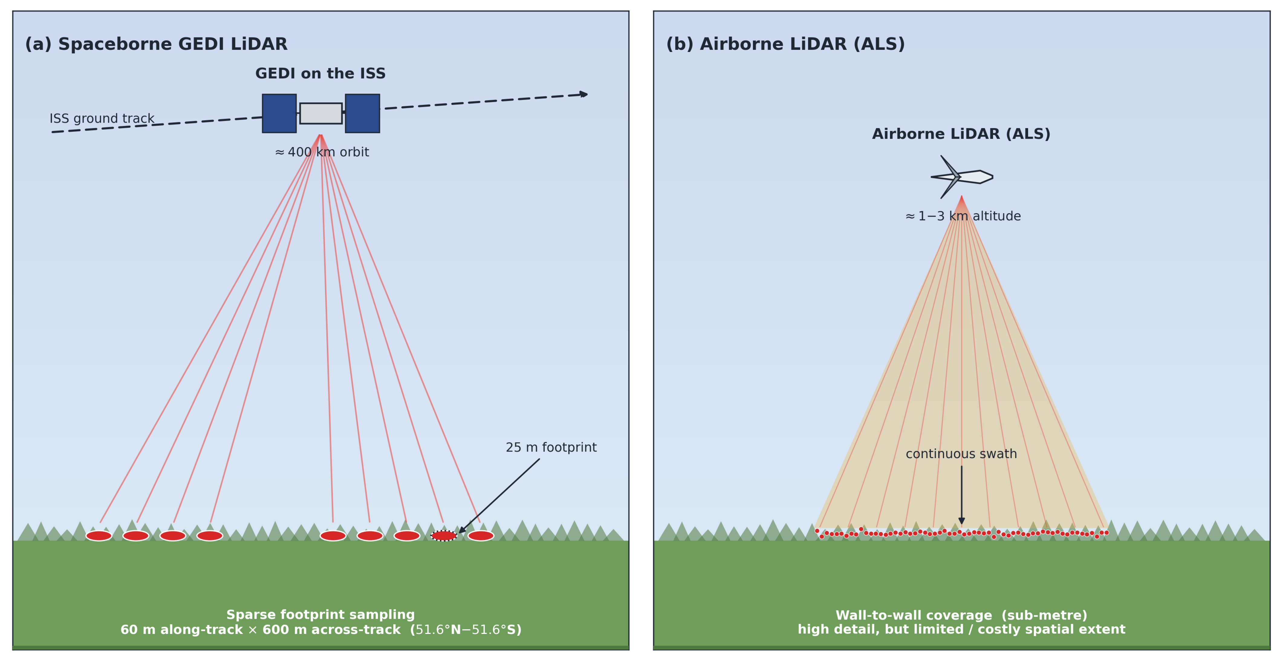
Figure 1. Acquisition geometry of spaceborne and airborne LiDAR. (a) GEDI, onboard the ISS (≈400 km altitude), collects sparse 25 m footprint samples spaced 60 m along-track and 600 m across-track, between 51.6°N and 51.6°S, and is therefore not spatially continuous. (b) Airborne LiDAR (ALS), flown at ≈1–3 km altitude, scans a continuous swath that yields submetre, wall-to-wall canopy measurements but over a limited and costly spatial extent.
Remotesensing 18 02477 g001
Figure 2. Study area in Ontario, Canada. Green shading delineates the Forest Resources Inventory (FRI) leaf-on airborne LiDAR (ALS) acquisition footprint, the dark blue line marks the Ontario boundary, and the dashed line marks GEDI’s northern observation limit at 51.6°N. The inset locates Ontario within North America.
Remotesensing 18 02477 g002
Figure 3. GEDI and high-resolution (HR) tiles spatial aggregation methodology. (A) Pipeline of the spatial aggregation strategy. (B) Illustration of the GEDI and ALS interception tiles. (C) Zonal statistics energy-based process to aggregate ALS samples to corresponding GEDI footprint resolution.
Remotesensing 18 02477 g003
Figure 4. Schematic representation of the proposed methodology. (A) Data acquisition process. (B) Data preprocessing strategy and training patch extraction. (C) Neural network optimisation procedure. (D) Inference approach using an ensemble of neural networks.
Remotesensing 18 02477 g004
Figure 5. Overview of the ResUNet network. (A) The left (downward) branch is the encoder part of the architecture; the right (upward) branch is the decoder. The last convolutional layer has as many channels as there are distinct outputs. (B) Building block of the ResUNet network. Each unit within the residual block has the same number of filters as all other units. (C) Combine block used to integrate encoder and decoder feature maps through concatenation followed by normed convolution.
Remotesensing 18 02477 g005
Figure 6. Assessment of agreement between GEDI RH98 and ALS-derived canopy-height statistics. Scatter plots with density colouring (warmer colours indicate higher point density) compare GEDI RH98 measurements with six ALS metrics: (a) 98th percentile, (b) 95th percentile, (c) 90th percentile, (d) median, (e) mean, and (f) maximum. Each panel shows the 1:1 reference line (dashed grey) and the linear fit (solid black), along with statistical metrics ( R 2 , RMSE, MAE, slope, and bias). Analysis based on 337,332 spatially co-located GEDI footprints and ALS tiles.
Remotesensing 18 02477 g006
Figure 7. Scatter plots of predicted canopy height versus the ALS-derived 98th-percentile reference for the headline configurations; the remaining optical-containing ablations and all SAR-only configurations are provided in Figures S4 and S5 (Supplementary Materials). (a) Gaussian and (b) Laplace NLL under identical inputs (W–S–F, LS–S1–AP–LL) with KDE inverse-density weighting; (c) the primary model W–S–F LS–S1–AP–X; (d) the SAR-only configuration W–S–F X–S1–AP–X; (e) the summer-only configuration X–S–X LS–S1–AP–X; and (f) the summer Landsat + Sentinel-1 configuration X–S–X LS–S1–X–X. The loss×weighting ablation is reported in Supplementary Figure S3.
Remotesensing 18 02477 g007
Figure 8. Relative change in RMSE ( Δ RMSE, %) and R 2 ( Δ R 2 , %) for each model configuration, benchmarked against the primary model (W–S–F LS–S1–AP–X). Blue bars represent the percentage increase in RMSE, while the red line shows the percentage decrease in R 2 . The plot summarises performance degradation across the seasonal, sensor, and covariate ablations, as well as GEDI and the four global products: Meta [30], Potapov et al. [21], Lang et al. [27], and Pauls et al. [28].
Remotesensing 18 02477 g008
Figure 9. Scatter plots comparing four global canopy-height products against the ALS P98 reference: (a) Meta [30], (b) Lang et al. [27], (c) Pauls et al. [28], and (d) Potapov et al. [21].
Remotesensing 18 02477 g009
Figure 10. (A) Distribution of ALS canopy-height values (0–40 m) used for validation. (B) Boxplots of prediction error (predicted − ALS P98) stratified into 5 m canopy-height bins. Compared models include the primary configuration (W–S–F LS–S1–AP–X), summer optical only (X–S–X LS–X–X–X), summer SAR fusion (X–S–X X–S1–AP–X), the Gaussian baseline, selected seasonal and summer SAR configurations, GEDI, and the four global products labelled Meta [30], Lang et al. [27], Potapov et al. [21], and Pauls et al. [28].
Remotesensing 18 02477 g010
Figure 11. Uncertainty calibration results for the primary model (W–S–F, LS–S1–AP–X). (a) Calibration curves before (uncalibrated, red) and after (calibrated, blue) Platt scaling, with the ideal 1:1 line (dashed black); the vertical dotted line marks the lower bound of the UCE evaluation range (≥2 m). (b) Distribution of calibrated uncertainty estimates. (c) RMSE versus recall after sorting samples by ascending calibrated uncertainty. (d) RMSE stratified by calibrated uncertainty quartile.
Remotesensing 18 02477 g011
Figure 12. Snapshots of three locations where GEDI and ALS canopy-height data intersect. Rows ((top) to (bottom), (ax)): satellite imagery with GEDI footprints; ALS reference (P98); Potapov et al. [21]; Meta [30] (P98); Lang et al. [27]; Pauls et al. [28]; ensemble estimate; calibrated uncertainty. Colour scale: 0–40 m for canopy height, 0–20 m for uncertainty.
Remotesensing 18 02477 g012
Figure 13. Forest-type stratified comparison of canopy-height products against the ALS reference (P98). (a) Grouped bar charts of R 2 , RMSE, MAE, and bias for seven products across four land cover classes. (b) Density scatter plots of the primary model predictions versus ALS P98, stratified by forest type, with regression statistics. (c) Boxplots of prediction error (prediction − ALS P98) by land cover class for all seven products. (d) Seasonal improvement ( Δ RMSE and Δ R 2 , computed as the relative difference between summer-only and seasonal configurations) for the optical (LS–S1–AP–X) and SAR-only (X–S1–AP–X) models, stratified by forest type. Land cover classes are derived from the 2020 North American Land Cover map (NALCMS, 30 m) [38]: coniferous (Conif.) ( N = 110,948 ), deciduous (Decid.) ( N = 51,814 ), mixedwood (Mixed) ( N = 123,622 ), and treed-wetland (Wetland+) ( N = 36,906 ). Mixedwood forests are defined as stands with intermingled deciduous and coniferous species. All evaluations use GEDI ∩ ALS intersection locations.
Remotesensing 18 02477 g013
Table 1. Summary of the input covariates supplied to UCNN. Landsat surface-reflectance bands and Sentinel-1 VV/VH backscatter are composited for three seasons (winter, summer, and fall), while annual composites are used for ALOS PALSAR-2 HH and HV observations. Geographic position is encoded with three spherical coordinates (latitude, sin ( π · lon / 180 ) , and cos ( π · lon / 180 ) ). When all data sources are available, each 30 m pixel is characterised by a maximum of 26 covariates.
FeaturesDetails
Landsat 7 & 8Type: Optical (multispectral)
Features: Blue, Green, Red, NIR, SWIR1
Temporal aggregation: Winter, Summer, Fall (3 seasons)
Covariates: 5 per season (15 total)
Notes: Standardised across sensors (Tier 1, SR)
Sentinel-1Type: C-band SAR
Features: VV, VH polarisation
Temporal aggregation: Winter, Summer, Fall (3 seasons)
Covariates: 2 per season (6 total)
Notes: Interferometric Wide swath, ascending pass
ALOS-PALSAR-2Type: L-band SAR
Features: HH, HV polarisation
Temporal aggregation: Annual composite
Covariates: 2 total
Notes: 1-year composite (2019–2020)
LocationType: Spatial features
Features: lat, sin ( π · lon / 180 ) , cos ( π · lon / 180 )
Temporal aggregation: Static
Covariates: 3 total (following [27] encoding)
Total26 covariates
Table 2. Summary of the four global canopy-height products used as benchmarks, as reported in the original publications.
ProductInput DataTargetNative Resolution
Meta [30]Commercial HR imageryALS-derived canopy top1 m
Lang et al. [27]Sentinel-2GEDI canopy height10 m
Potapov et al. [21]Multi-temporal Landsat-8GEDI RH9530 m
Pauls et al. [28]Sentinel-1 + Sentinel-2GEDI (shift-tolerant)10 m
Table 3. Glossary of the notation used to label experimental configurations throughout the paper. Each configuration is identified as (temporal pattern)–(sensor/geographic pattern); a token of X marks an omitted component.
TokenMeaning
Temporal pattern (3 tokens)
WWinter composite included (Jan–Mar)
SSummer composite included (Jun–Aug)
FFall composite included (Sep–Nov)
Sensor/geographic pattern (4 tokens)
LSLandsat (B, G, R, NIR, SWIR1) included
S1Sentinel-1 (VV, VH) included
APALOS-PALSAR-2 (HH, HV) included
LLLatitude/longitude coordinates included
XCorresponding component omitted
Table 4. Canopy-height estimation accuracy for every experimental configuration, GEDI RH98, and the four global products against the ALS P98 reference. Configurations are labelled (temporal pattern)–(sensor/geographic pattern) following Table 3; all use the Laplace NLL with KDE inverse-density weighting unless noted. Bias is predicted − observed and slope is that of the predicted-versus-observed regression line.
Configuration R 2 RMSE (m)MAE (m)Bias (m)Slope
All-season optical-containing (W–S–F)
W–S–F LS–S1–AP–X a0.703.652.730.230.88
W–S–F LS–S1–AP–LL0.703.642.720.140.87
W–S–F LS–S1–X–LL0.693.672.760.070.83
W–S–F LS–S1–X–X0.683.742.810.270.87
W–S–F LS–X–X–X0.653.912.980.420.84
W–S–F LS–S1–AP–LL (Gaussian)0.594.223.231.430.79
All-season SAR-only (W–S–F)
W–S–F X–S1–AP–X0.653.943.010.710.80
W–S–F X–S1–AP–LL0.643.953.010.810.79
W–S–F X–S1–X–X0.604.183.200.890.77
W–S–F X–S1–X–LL0.574.333.331.170.77
Yearly X–X–AP–X b0.584.303.37−1.050.61
Yearly X–X–AP–LL b0.574.363.42−1.400.59
Summer-only (X–S–X)
X–S–X LS–S1–AP–LL0.634.053.060.880.84
X–S–X LS–S1–AP–X0.624.093.100.950.86
X–S–X LS–S1–X–LL0.624.063.070.690.80
X–S–X LS–S1–X–X0.634.053.070.700.82
X–S–X LS–X–X–X0.544.483.440.880.75
X–S–X X–S1–AP–X0.584.303.291.270.80
X–S–X X–S1–AP–LL0.574.353.311.280.79
X–S–X X–S1–X–LL0.524.613.521.120.68
X–S–X X–S1–X–X0.484.763.621.660.73
Reference and global products
GEDI RH980.604.212.93−1.110.89
Pauls et al. [28]0.584.283.28−1.730.65
Lang et al. [27]0.514.633.521.550.61
Potapov et al. [21]0.096.324.91−3.890.63
Meta [30]−0.167.146.03−5.680.74
a Primary model adopted for all subsequent analyses. b Yearly ALOS-PALSAR-2 mosaic configurations (no seasonal compositing).
Disclaimer/Publisher’s Note: The statements, opinions and data contained in all publications are solely those of the individual author(s) and contributor(s) and not of MDPI and/or the editor(s). MDPI and/or the editor(s) disclaim responsibility for any injury to people or property resulting from any ideas, methods, instructions or products referred to in the content.