Article

Monitoring Coastal Surface Roughness Suppression Associated with Algal Blooms and Pollutants Using NASA SWOT Observations


Department of Climate and Space Sciences and Engineering, University of Michigan, Ann Arbor, MI 48109, USA
*
Author to whom correspondence should be addressed.
Remote Sens. 2026, 18(15), 2464; https://doi.org/10.3390/rs18152464
Submission received: 17 May 2026 / Revised: 20 July 2026 / Accepted: 22 July 2026 / Published: 27 July 2026

Highlights

What are the main findings?
  • NASA SWOT radar observations can detect changes in ocean surface roughness related to algal blooms
  • An estimator of algae concentration derived from SWOT observations broadly matches measurements by NOAA VIIRS
What are the implications of the main findings?
  • SWOT algae estimates can complement measurements by optical sensors in cloudy conditions
  • The approach opens opportunities to broader marine pollution monitoring due to SWOT’s sensitivity to ocean surface roughness

Abstract

Marine litter accumulation in aquatic ecosystems presents a dire problem for marine life and the human ecosystem. The presence of algae on the ocean surface can alter its response to wind-driven roughening. This alteration is the basis for a new method to detect and image algae and other roughness suppression inducing pollutants from space. The NASA Surface Water and Ocean Topography (SWOT) radar can measure coastal ocean roughness. An empirical model is developed which relates the Mean Square Slope (MSS), a measure of ocean surface roughness, to wind speed given clear water conditions. Deviations of the roughness observed by SWOT from the clear water model results in roughness anomalies that are found to be empirically associated with the concentration of chlorophyll-a observed by the NASA VIIRS instrument. The relationship between roughness anomaly and chlorophyll concentration is incorporated into a new retrieval algorithm for algae by SWOT. This retrieval algorithm has a valid range of 0–6 mg/m3.

1. Introduction

1.1. Introduction to Algal Blooms

Algae are accumulations of phytoplankton that proliferate when sufficient sunlight coincides with elevated nutrient availability. These nutrients are most often supplied by runoff delivered through watersheds. When this accumulation occurs in an uncontrolled manner and reaches a high biomass over a broad area, it is commonly characterized as an algal bloom [1]. Such blooms occur across a wide range of marine environments including rivers, lakes and the open ocean. Algal blooms frequently concentrate along coastlines adjacent to major river outflows, where nutrient inputs and physical transport processes can promote sustained growth and aggregation [2].
Algal blooms can degrade marine ecosystem health [3]. Dense blooms may contribute to oxygen depletion in the water column, killing fish and other organisms through hypoxic conditions [4]. In addition, bloom events can impair drinking water supplies and may produce toxins that pose risks to human health through exposure or consumption of contaminated water or seafood [4]. Therefore, reliable detection and monitoring of algal blooms are essential.
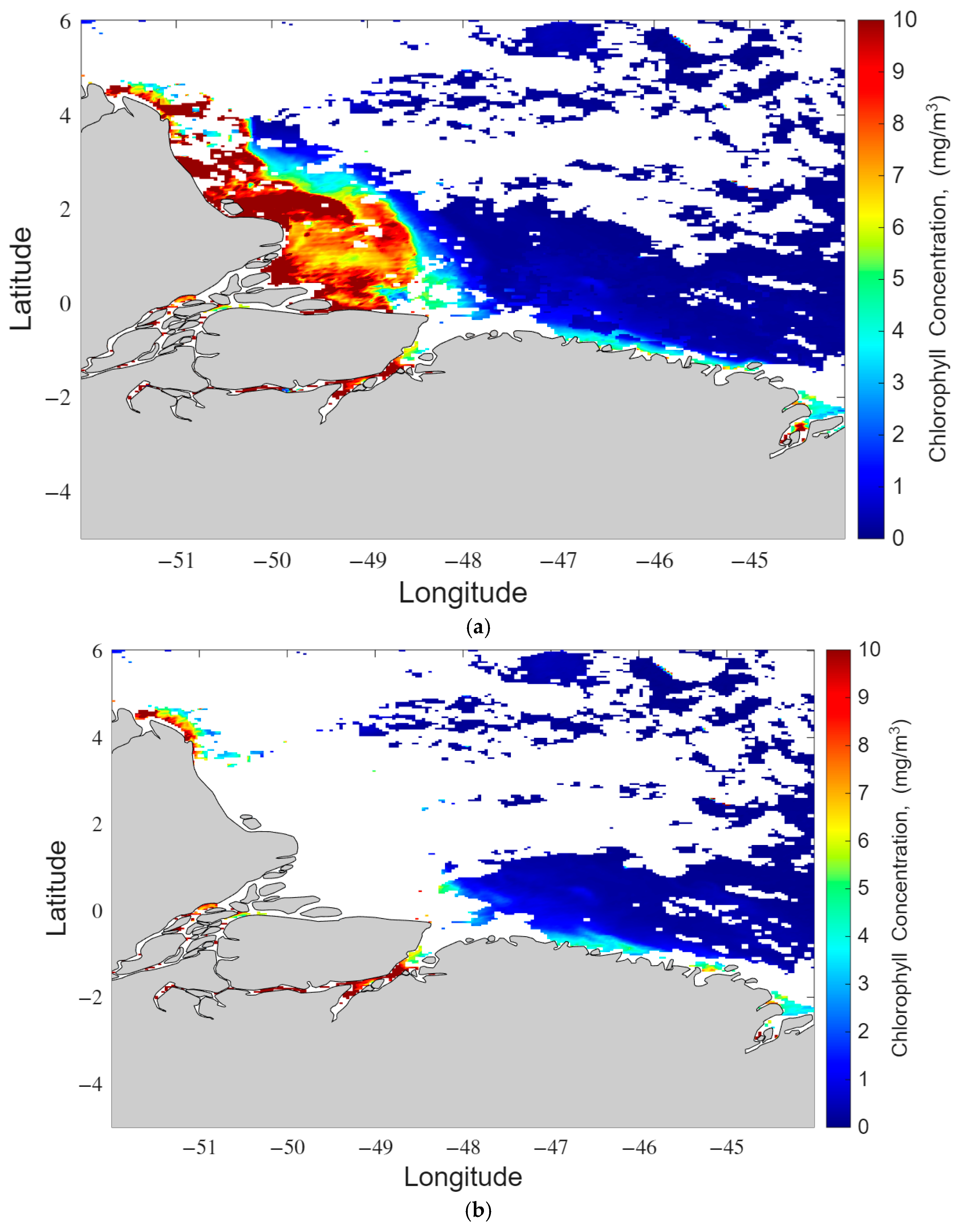
Traditional remote-sensing approaches often rely on optical or hyperspectral imaging, using the distinct spectral signatures associated with chlorophyll and related pigments. Many detection algorithms emphasize the green portion of the spectrum (around 532 nm), where reflectance and absorption features can help parse algal blooms from surrounding waters [5]. NOAA’s Visible Infrared Imaging Radiometer Suite (VIIRS) chlorophyll-a product is an example of a hyperspectral imager data product [6]. Figure 1 is a set of example images from VIIRS over the Amazon River in 2024.
Figure 1 demonstrates both the strengths and weaknesses of the VIIRS product. As shown in Figure 1a, the 2 km resolution of the product can describe algal bloom structure in detail. However, Figure 1b shows that cloud cover frequently obscures visible wavelengths from observing the ocean surface, preventing the acquisition of spatially and temporally continuous (gap-free) observations. To mitigate this limitation, we consider algal bloom detection in the microwave regime, where longer wavelengths can penetrate clouds and enable more consistent observing conditions, providing a pathway to more reliable bloom monitoring when optical data are unavailable.

1.2. Microwave Imagers

Microwave imagers are instruments that take measurements at frequencies between 0.3 GHz and 300 GHz. Below 0.3 GHz lie HF and VHF radio waves and above 300 GHz is the sub-mm and far infrared portion of the electromagnetic spectrum.
An example of a microwave imager useful for coastal ocean pollutants is Synthetic Aperture Radar (SAR). SAR can be effective for accurate coastal pollutant detection [7,8]. SAR has been used to monitor and identify oil spills on the ocean surface [9]. Its detection mechanism leverages the suppression of capillary and short-gravity capillary waves caused by oil spills, which reduces the surface roughness.
Another example of microwave imagers is the NASA Cyclone Global Navigation Satellite System (CYGNSS) mission. CYGNSS uses a constellation of eight small satellites to study tropical cyclones and improve understanding of hurricane intensification. CYGNSS uses GNSS Reflectometry (GNSS-R), a passive bistatic radar technique [10]. Instead of transmitting its own pulses, CYGNSS measure GPS signals after they reflect off the ocean surface. CYGNSS infers properties of the sea surface, most notably surface roughness, which is closely related to near-surface wind speed [11]. Roughness suppression in the case of CYGNSS has been associated with the concentration of microplastics in the open ocean [12,13].

1.3. The NASA Surface Water & Ocean Topography (SWOT) Mission

Here we consider an application of the ocean roughness suppression approach used by CYGNSS to the detection of algae in coastal waters. Due to the coarse (~25 km) spatial resolution of CYGNSS, we consider use of the high-resolution NASA Surface Water & Ocean Topography (SWOT) Mission’s radar [14]. SWOT carries a Ka-Band (8.6 mm wavelength) altimetric radar and its primary mission objective is water surface height topography. However, it also makes ocean surface roughness measurements (specifically, normalized radar scattering cross section, σ0) as a secondary correction for sea surface height. SWOT’s Low-Rate Sea Surface Height Data Product has a resolution of 2 km in both the cross-track and along-track directions [14]. This improved spatial resolution enables observations much closer to the coastline.
SWOT’s temporal revisit time is a notable limitation. The SWOT orbit has a repeat cycle of 21 days [15], and SWOT’s average image revisit time of 11 days will restrict the ability to monitor rapid changes in coastal ocean litter distributions.

2. Materials and Methods

The CYGNSS algorithm is based on the principle that ocean pollutants cause sufficient ocean surface roughness suppression to be measurable by the satellite. Surface roughness is characterized by its Mean Square Slope (MSS), which is the expected value of the square of surface slope, averaged over the spectrum of ocean surface height at different horizontal scales [16]. To parameterize ocean roughness suppression, a Mean Square Slope Anomaly (MSS Anomaly) parameter was developed. This approach will be adapted for use with SWOT observations.

2.1. Dataset Description Table

Before developing the approach, a dataset description table is listed. Throughout this study, various datasets are used, ranging from reanalysis data products to spaceborne radar products. Table 1 consolidates all products used, and includes spatial resolution, temporal resolution and coverage period.

2.2. Deriving the Forward Model: A Mathematical Approach to MSS Anomaly

MSS Anomaly is a derived product that describes how different the ocean roughness is from a modeled “normal” version of ocean roughness forced by near-surface ocean wind. A negative MSS Anomaly indicates that the observed roughness is lower than the wind-predicted roughness, implying surface suppression. Global maps of MSS Anomaly illustrate areas where ocean roughness suppression occurs, which is hypothesized to be directly caused by surfactant concentrations and indirectly correlated with microplastic and algal bloom concentrations.
M S S A N O M = M S S o b s M S S m o d M S S m o d ,
where MSSobs is the observed MSS from satellite data and MSSmod is a theoretical MSS value calculated using an empirical MSS model forced by ECMWF Reanalysis (ERA5) wind speed data [17]. The model was constructed from MSS observations and wind data taken from a clean ocean region free from contaminants and anomalous conditions.
The MSS observations themselves are calculated using
M S S o b s = | R ε , θ | 2 σ 0 ,
where R(ε, θ) is the Fresnel Reflection Coefficient and σ0 is the normalized radar cross section [18]. σ0 is measured by the SWOT radar and is notably sensitive to near-surface wind speed. SWOT pixels flagged for degraded σ0 quality and precipitation were excluded before MSS Anomaly calculations.
The Fresnel Reflection Coefficient is a function of the relative dielectric permittivity of seawater (ε) and the incidence angle of the satellite observation (θ), as given by [19]
R ϵ ,   θ = 1 2   [ ϵ f , T , S cos θ ϵ sin 2 θ ϵ cos θ + ϵ sin 2 θ cos θ ϵ sin 2 θ cos θ + ϵ sin 2 θ   ] ,
The permittivity is also a function of sensor transmitter frequency, sea surface temperature (SST) and sea surface salinity (SSS) conditions of the ocean. For our calculations, we use the Double Debye model as described in [20]. The Fresnel Reflection Coefficient calculated in Equation (3) is used to calculate the MSS in Equation (2). The incidence angle range used evaluates the full range of SWOT data, from 0.8° to 4°, and is discussed further in Appendix A.
In summary, MSS Anomaly is derived from measurements of σ0 and estimates of the Fresnel Reflection Coefficient. Determination of the Fresnel Reflection Coefficient requires knowledge of ε, which in turn requires knowledge of SST and SSS. Therefore, to develop a SWOT MSS and MSS Anomaly estimator, the process requires matching σ0 data to collocated SST and SSS data.

2.3. Using the SWOT Product to Calculate MSS

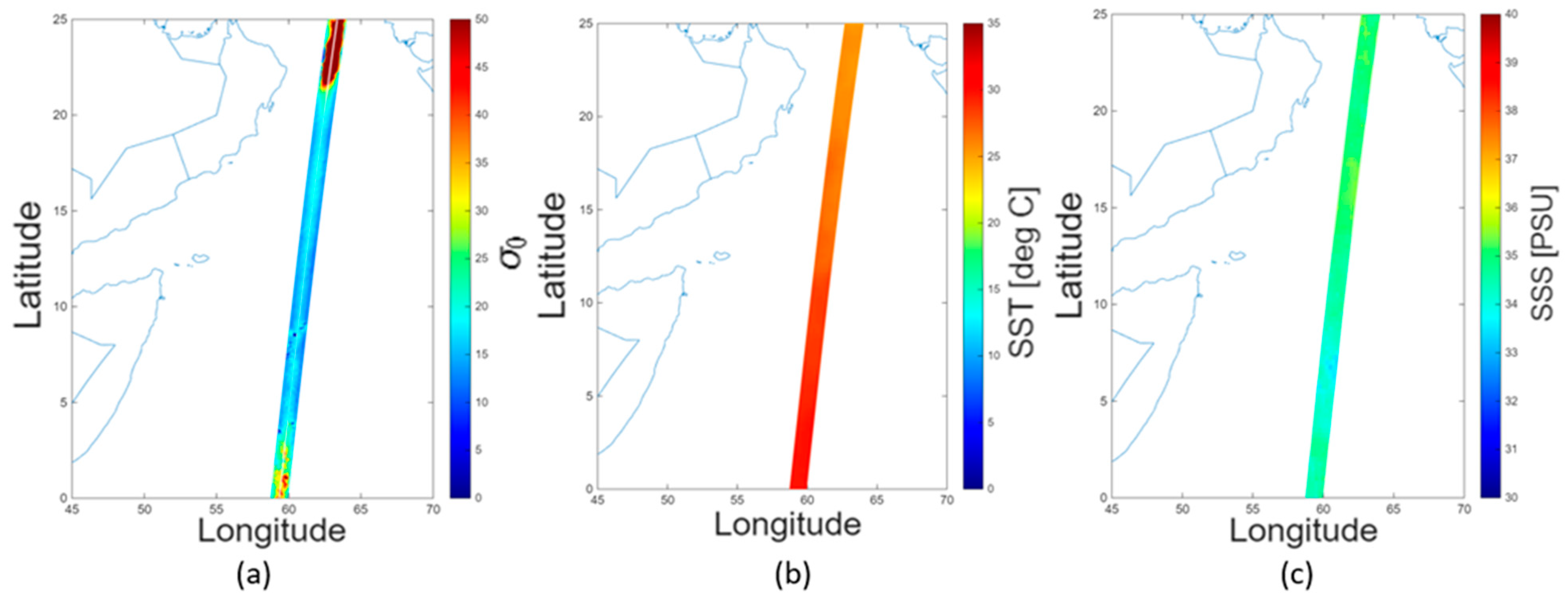
An example of one SWOT orbital pass of σ0 data collocated with SST and SSS provided by ERA5 [21] and SMAP [22] is shown in Figure 2.
Combining the SST and SSS inputs (see Figure 2b,c) allows us to obtain the Fresnel Reflection Coefficient described in Equation (3). Combining the Fresnel Reflection Coefficient with the σ0 paths in Figure 2a results in the MSS described in Equation (3). See Appendix A for a description of how the ERA5 and SMAP data are used to create the Fresnel Reflection Coefficient. Collocation was performed by matching each 2 km SWOT pixel to the nearest ERA5 grid cell and nearest hourly time step. The maximum temporal mismatch was therefore 30 min. The same procedure was applied from SWOT to the SMAP SSS. Because SMAP SSS is provided as an 8-day running product, it may smooth rapidly evolving salinity gradients near river mouths. However, Appendix A shows that SSS variations have a negligible effect on the Fresnel Reflection Coefficient relative to the other sources. Therefore, use of the 8-day product is not expected to affect MSS Anomaly estimates. A full description of the implications of mixed-spatial grid matching is in Section 5.3. SST and SSS were collocated to each SWOT σ0 pixel using the nearest spatial grid cell and nearest available time step. Because ERA5 and SMAP are substantially coarser than SWOT, higher-order interpolation would not recover sub-grid variability and could introduce a misleading level of spatial detail. Appendix A shows that the direct effects of SST and SSS on the Fresnel Reflection Coefficient are small compared with the σ0 and wind-speed dependence of MSS. Therefore, nearest-neighbor collocation was used as a practical and transparent approach. No resampling of the ERA5 or SMAP data was done, leaving it on its native 0.2° resolution, which is indicated through the homogeneity in Figure 2b,c.

2.4. Developing SWOT MSS Anomaly

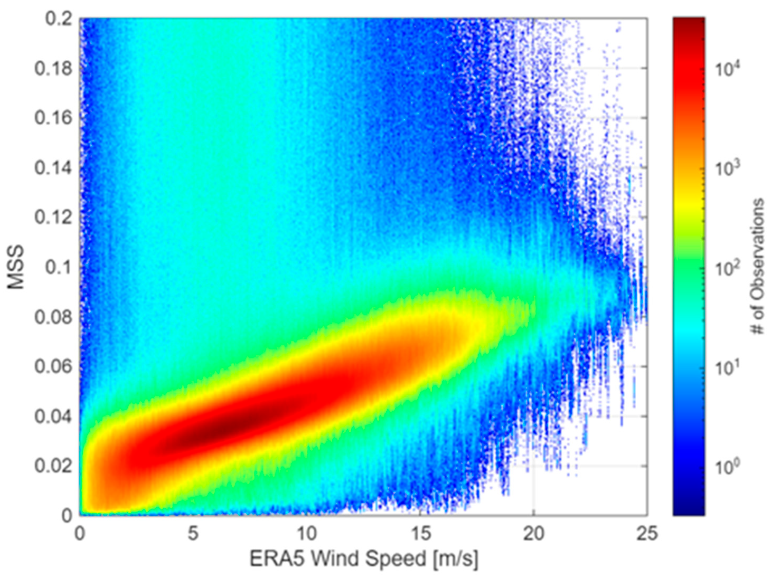
Using the Lookup Table Fresnel Reflection Coefficients described in Appendix A, the SWOT MSS estimator was implemented for the testing period of 1 January 2024 to 31 December 2024. Figure 3 below is a density scatter plot of ERA5 Wind Speed matched up with SWOT MSS from 1 January 2024 to 31 January 2024.
Figure 3’s results are a positive indication that the matchups are working, as with an increase in wind speed there is an increase in MSS.

2.5. Developing the MSS Model (MSSmod) for MSS Anomaly (MSSANOM)

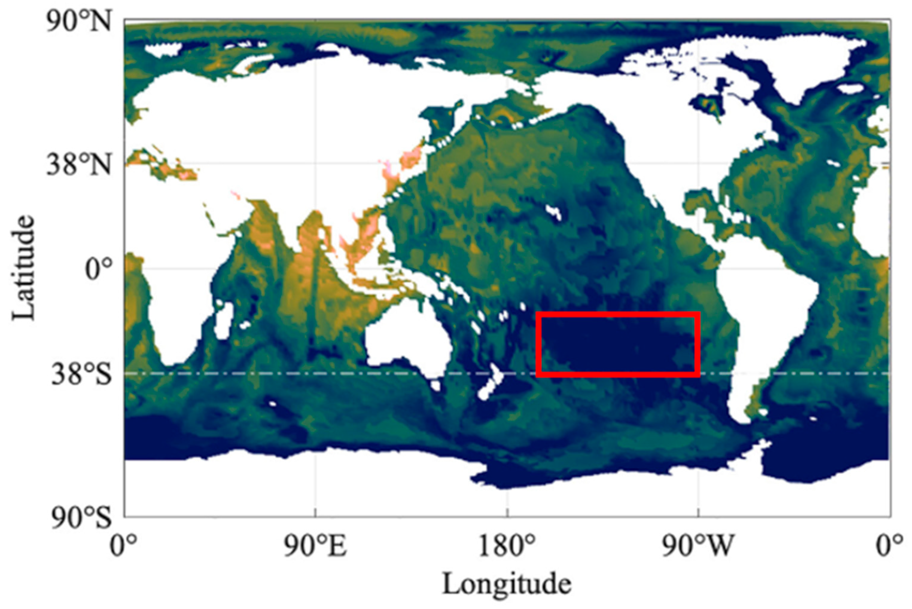
A control region is selected using microplastic models to find an area of open ocean that is clean of marine litter (microplastics, algae, sargassum). In this case the 3D model from Tseng et al. [23] was used to help find a viable control region. Figure 4 is a global map of high-density PVC concentration. The control region [28°–38°S, 200°–260°E] used is boxed in red.
Although the region is not perfectly free from plastic pollution, it is one of the cleaner areas when looking across the globe. This region is devoid of algae and seaweed though, as it is too far out in the middle of the Pacific Ocean to sustain growth for either. From here, our MSSmod can be built.

2.6. Cross-Track off Specular Point Geometry

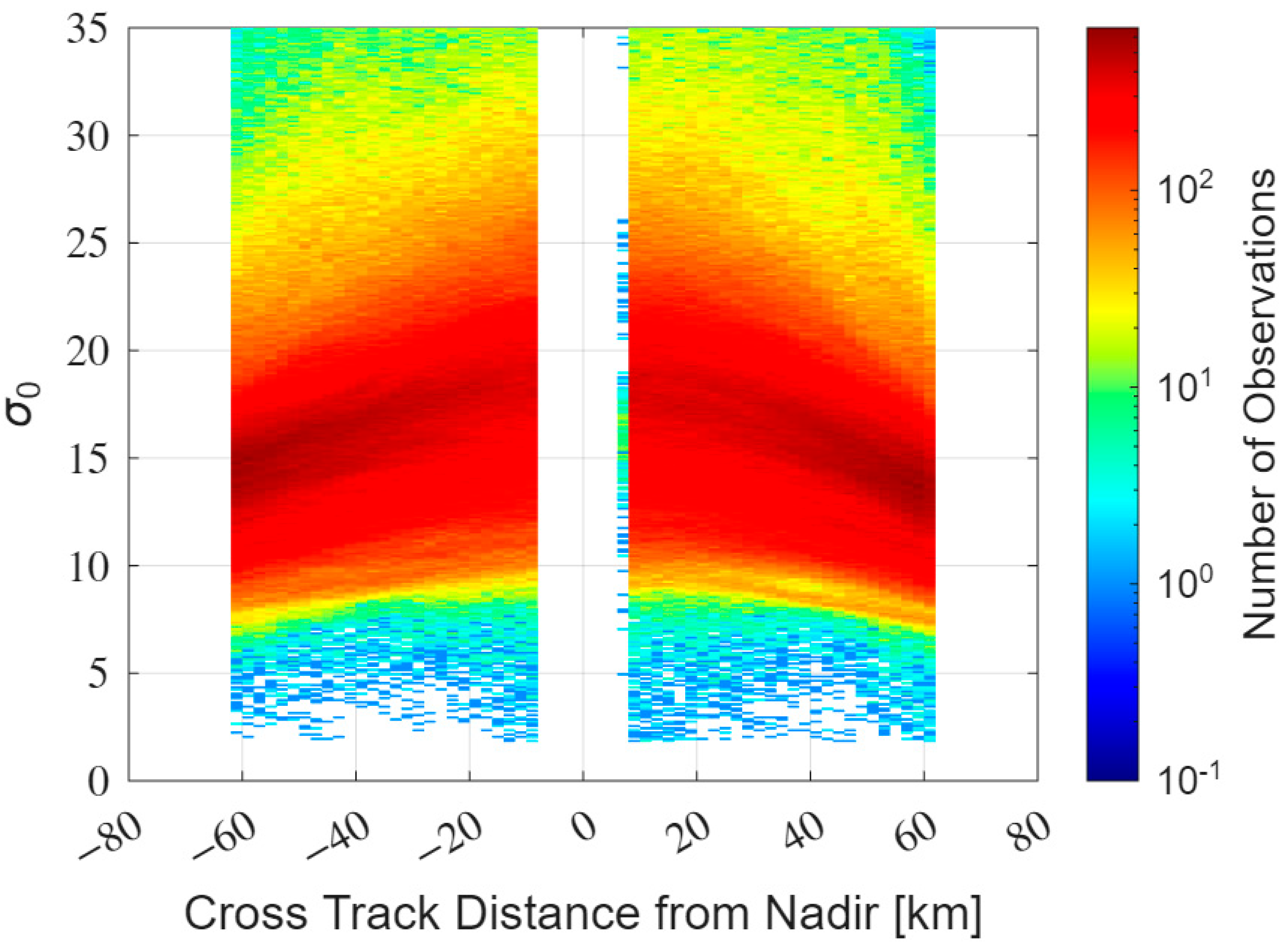
One of the main reasons why Equation (3) is simplified is because it assumes that the geometry of the transmitter and receiver are looking at the specular point [18]. For SWOT, nadir is where the specular point is located. The drop-off from the specular point in terms of power is quite drastic, even over a couple of kilometers [18]. Therefore, the signal strength of σ0 decreases with cross-track distance from nadir. Figure 5 is a density scatter plot from the previously defined control region [200°–260°E, 28°–38°S] of cross-track distance from nadir and σ0.
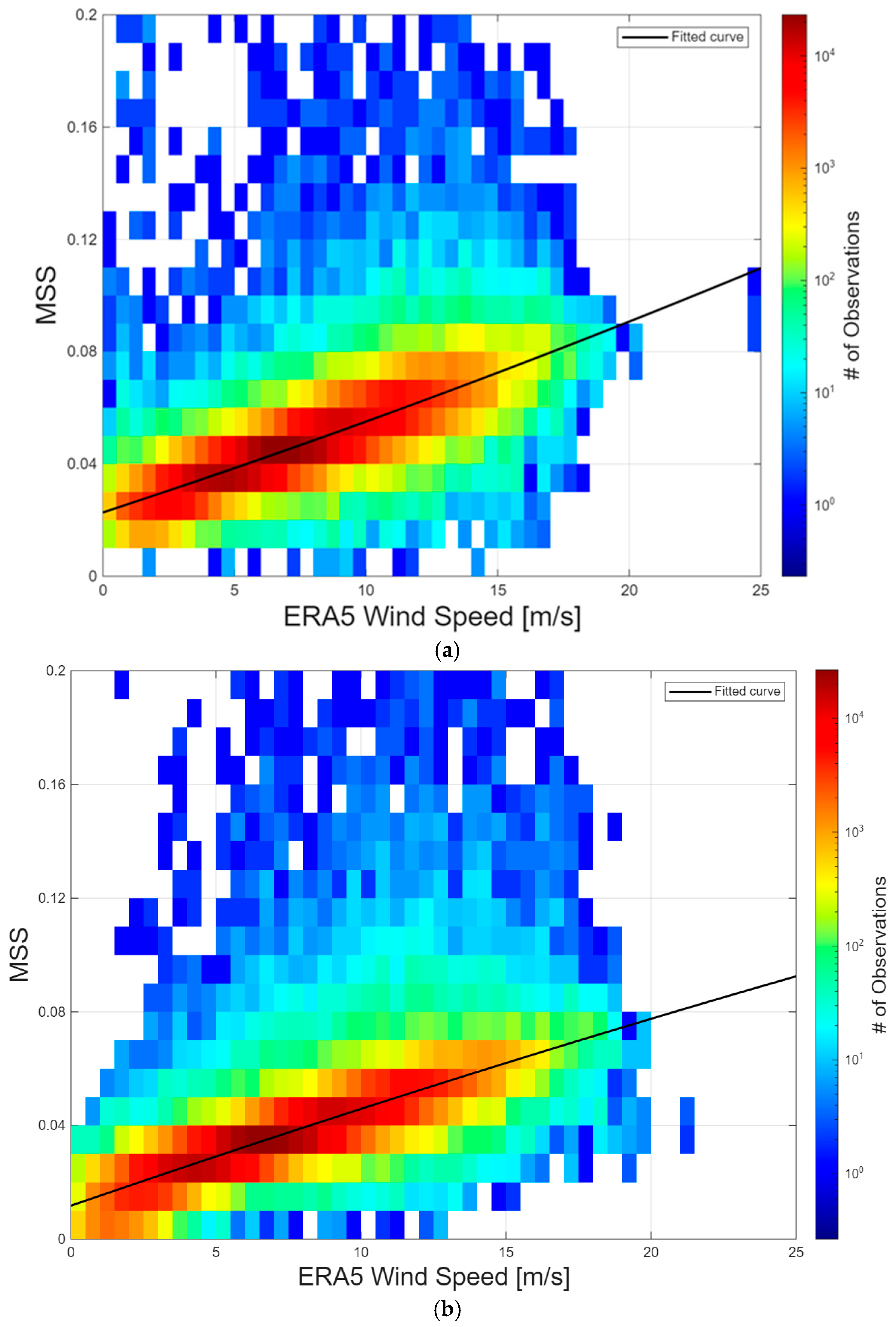
Because of the correlation between cross-track distance and σ0 the method of creating MSSmod must be customized as a function of cross-track location. The cross-swath structure in σ0 is not interpreted as a geophysical gradient in roughness alone. It is strongly affected by SWOT viewing geometry and incidence-angle dependence, with systematic variation away from nadir. This motivates the construction of the MSS model as a function of both wind speed and cross-track location before calculating MSS Anomaly. All data are binned every 2 km of cross-track distance, and an individual model is created for each bin. Two examples of MSS vs. Wind Speed are given below; Figure 6a is data from the bin closest to nadir, and Figure 6b uses data from the bin furthest from nadir.
The best-fit curves shown in Figure 6 represent the MSS model used to map wind speed to MSS. The equations for the model take the form of
M S S m o d C T = a C T U 2 + b C T U + c ( C T ) ,
where MSSmod is the modeled MSS for a given wind speed, U is wind speed, CT is cross-track distance from nadir and a(CT), b(CT) and c(CT) are constants that depend on the cross-track bin. a(CT) has units of s2/m2, b(CT) has units of s/m, and c(CT) is unitless.
From this, Equation (1) is modified so each observation of MSS is converted into MSSANOM using the appropriate MSSmod, described as
M S S A N O M = M S S o b s C T M S S m o d C T M S S m o d ( C T ) ,
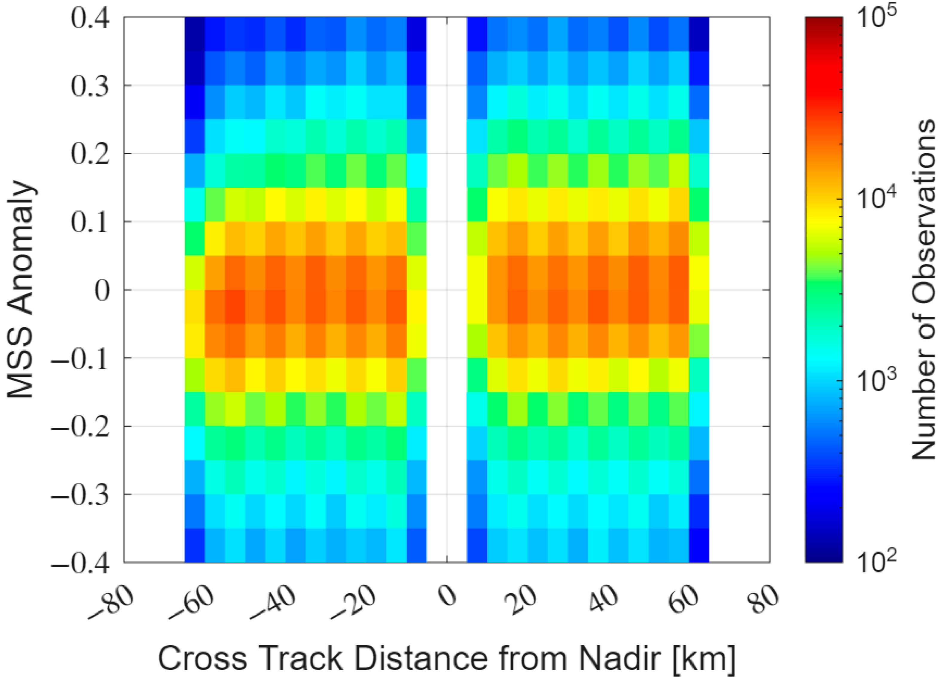
Modifying Equations (1)–(5) allows MSSANOM to be cross-track independent, which is seen in Figure 7. Figure 7 is a density scatter plot of MSSANOM in the control region compared to cross-track distance from nadir.
As can be seen in Figure 7, the distribution of MSSANOM is no longer cross-track-dependent. Therefore, MSSANOM measurements can now be used in conjunction with VIIRS gap-filled chlorophyll-a data to train a SWOT MSSANOM-Algae Model.

3. Amazon River Model Training Case

3.1. Choosing a Region and Initial Filtering of the Data

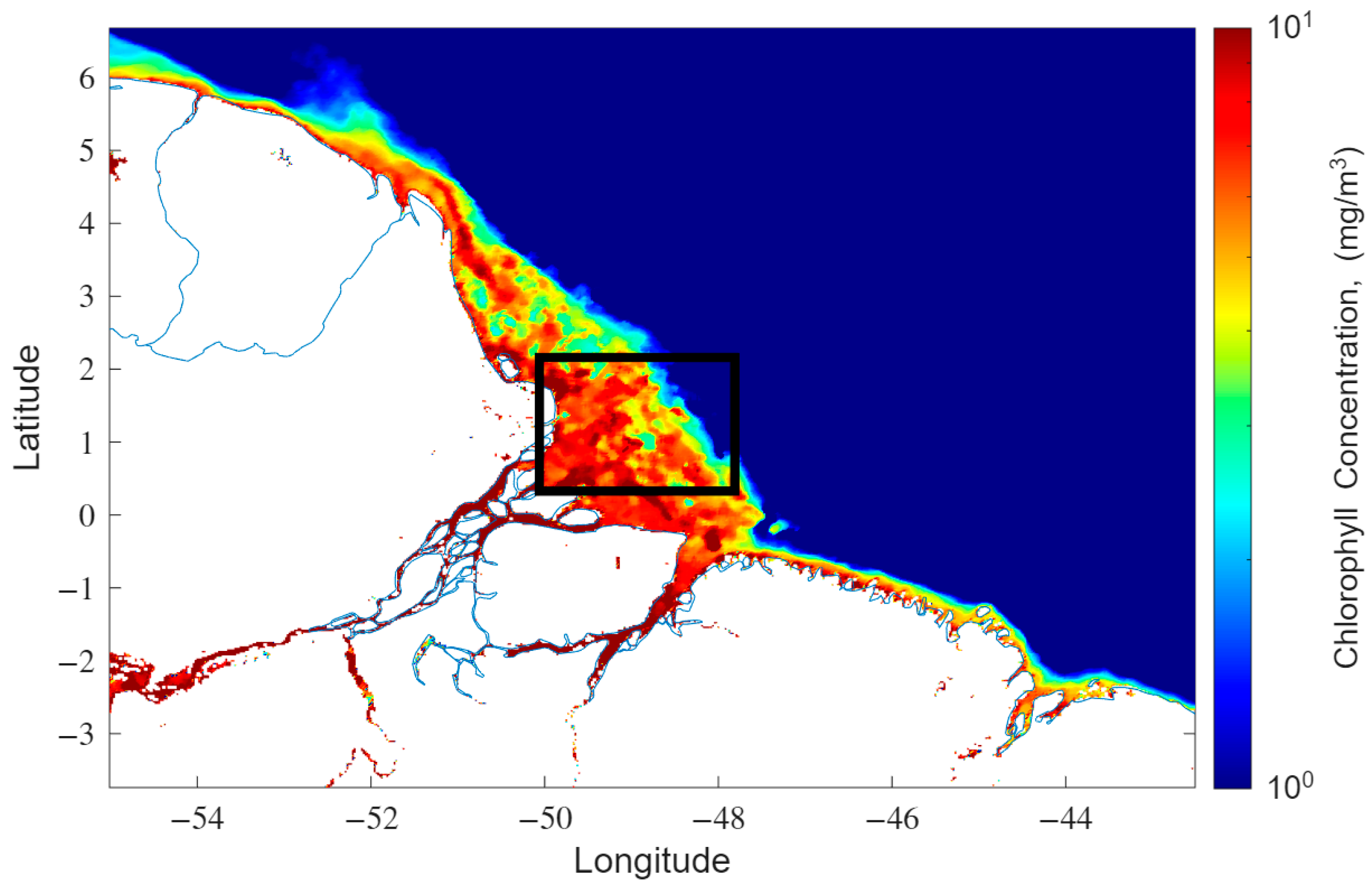
Using 2024 NOAA VIIRS 2 km gap-filled chlorophyll-a data [24], regions of high chlorophyll-a concentration can be identified throughout the year. Coastal areas generally have consistent background levels of chlorophyll-a, making them less likely to display dramatic short-term changes compared to offshore algal bloom events. However, there are some areas with larger dynamic ranges of chlorophyll-a near coastlines that are good candidates for SWOT MSS-Algae Model training. The first region of interest is at the mouth of the Amazon River. A snapshot of the Amazon River mouth with the region used for training highlighted by the box is shown in Figure 8.
The boxed region [0.6354°–2.22°N, 48.01°–49.76°W] in Figure 8 represents the area in which chlorophyll-a and SWOT will be examined to see if there is a relationship between MSSANOM and chlorophyll-a data.
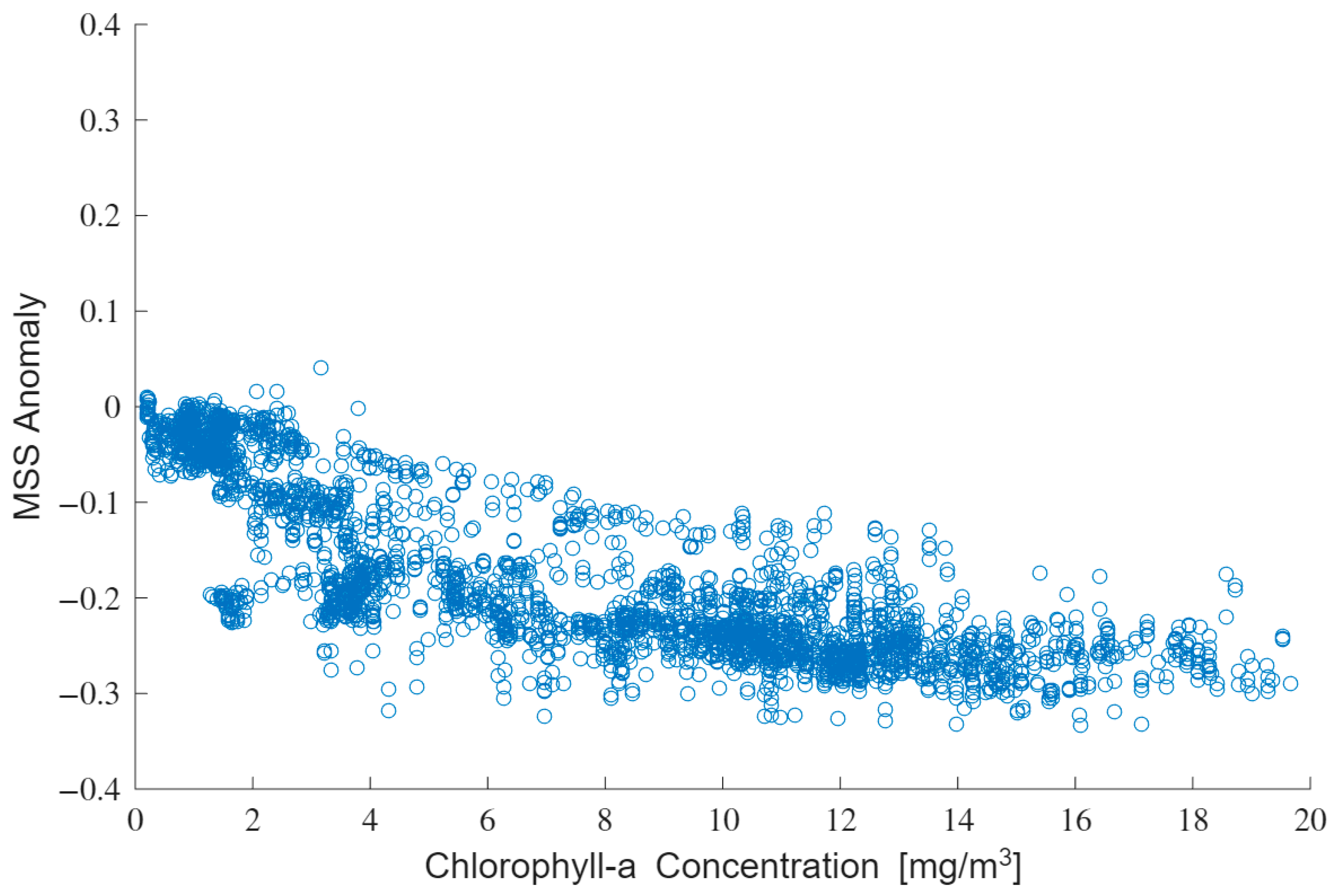
A total of 100 SWOT overpasses occurred in the testing region during calendar year 2024. An example of one of the SWOT overpasses matched up with VIIRS chlorophyll-a data is illustrated in Figure 9. Figure 9 is a scatter plot between chlorophyll-a concentration on the x-axis and MSSANOM on the y-axis. Each data point represents one 2 km SWOT pixel matched with its nearest 2 km grid cell in the VIIRS data.
Figure 9 is a good representation of some of the qualities needed to establish a model between MSSANOM and chlorophyll-a data.
  • The minimum requirements for inclusion in the training dataset are as follows
(1)
The overpass should capture a sufficiently wide range of chlorophyll-a values, which is quantified by a standard deviation equal to or greater than 2.5 mg/m3.
(2)
The overpass must consist of at least 500 points of data.
These filtering criteria reduced the dataset from 100 overpasses to 35. In total, 54 of the overpasses fail to meet the dynamic range threshold, and 56 of the overpasses fail the sample number threshold. Further evaluation of the remaining overpasses revealed that, while linear fits provided reasonable model performance, a quadratic regression gave superior results for most cases. The assumption of a quadratic relationship between concentration and MSS Anomaly is consistent with previous wave tank experiments we conducted in which controlled algae concentration were introduced and the resulting suppression of water surface roughening from wind was observed [25]. The wave tank experiment simulated ocean waves in a 35 m wind-wave tank, using a fan to generate wind speeds of 5.26, 7.83, and 10.34 m/s while ultrasonic surface sensors measured water height to derive Mean Square Slope (MSS) via the second moment of the wavenumber spectrum. Six chlorophyll-a concentrations (0–8 mg/m3), created using the microalga Nannochloropsis oculata as a proxy for algal biomass, were tested at each wind speed to see how algae presence affects surface roughness. Clean-water baseline runs validated the measurement approach against prior tank studies, and the team characterized key uncertainties from instrument precision, fan repeatability, and chlorophyll preparation/measurement. The controlled tank experiment demonstrates that algal material can suppress short-wave surface roughness under simplified conditions. However, this result does not by itself establish that all MSS suppression observed in natural river-plume environments is caused by algae. In coastal waters, chlorophyll-a can co-vary with sediments, dissolved organic matter, surfactants, oils, floating debris, salinity gradients, and convergence zones, any of which may also modify surface roughness. Therefore, the SWOT MSS anomaly should be interpreted as an indicator of surface roughness suppression that may be associated with algal biomass under favorable conditions, rather than as an exclusive or causal measure of chlorophyll-a.
The results showed that MSS consistently decreased as chlorophyll concentration increased at each wind speed, indicating that algae dampens surface roughness. Linear regressions of MSS vs. chlorophyll concentration were fit separately for each wind speed, and the resulting slopes and intercepts were combined into a three-parameter MSS–Wind Speed–Chlorophyll Concentration (MWCC) model: MSS = a(WS)·CC + b(WS), where a(WS) and b(WS) are linear functions of wind speed. The model revealed that MSS depends strongly on wind speed and more weakly, but measurably, on chlorophyll concentration, a relationship likely muted by tank-specific limitations. Despite this attenuation, the consistent chlorophyll signal supported the premise that biological presence measurably affects MSS and established a functional structure (an algae-indicator term plus a scaling term) later applied to the satellite-based CYGNSS/VIIRS analysis.
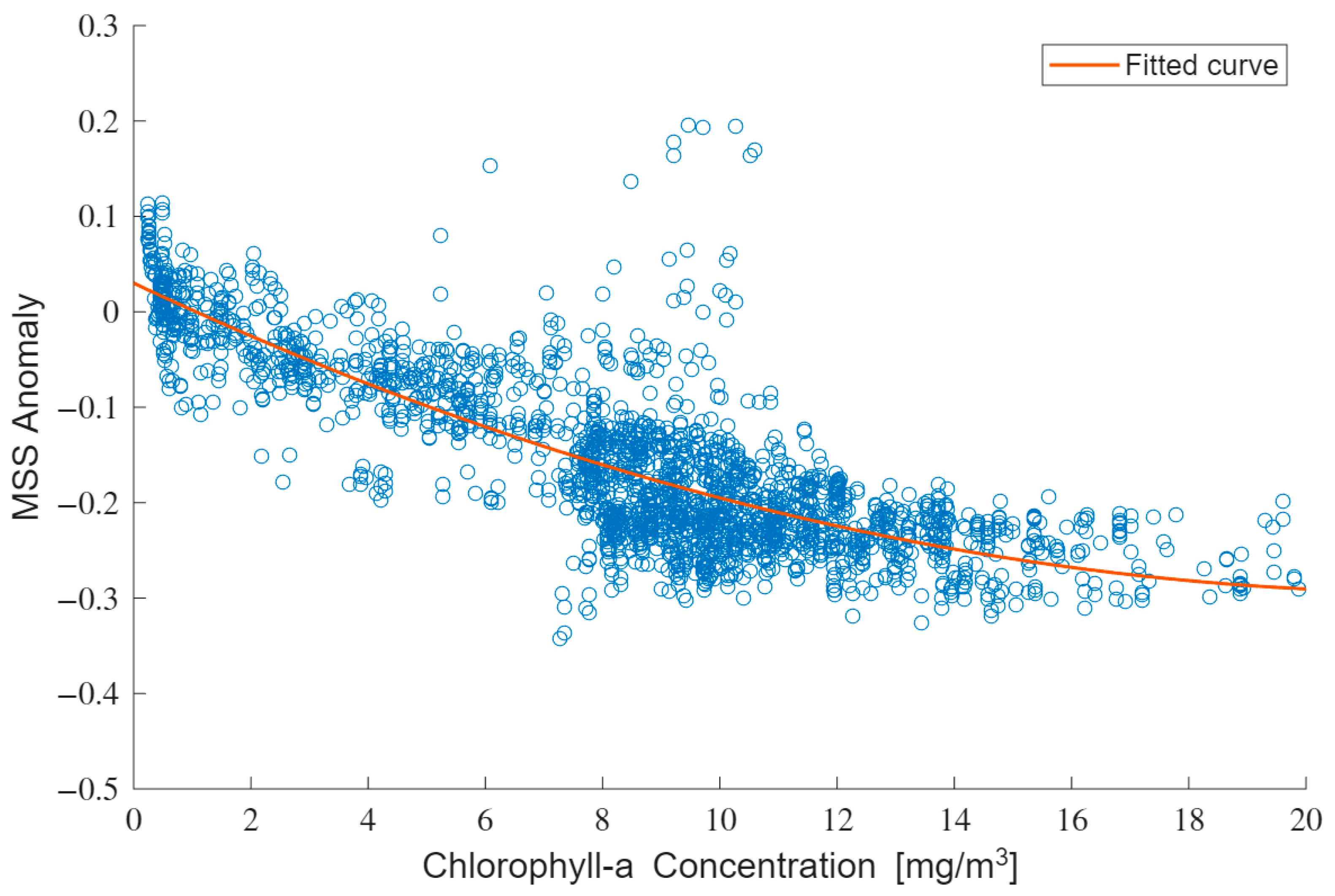
Specifically, the application of a quadratic fit improved the R2 value for all but one overpass, suggesting a more appropriate modeling approach for the relationship between MSSANOM and chlorophyll-a. Examples of the SWOT overpasses with quadratic fits overlaid on them are shown in Figure 10.
The quadratic fits in Figure 10 assumes a relationship of the form
M S S A N O M = a C C 2 + b C C + c ,
where CC is chlorophyll-a concentration and a, b and c are constants that are unique to each overpass. The units of a are m6/mg2, b are m3/mg and c are unitless.

3.2. Filtering the Overpasses Further to Make the SWOT MSSANOM-Algae Model

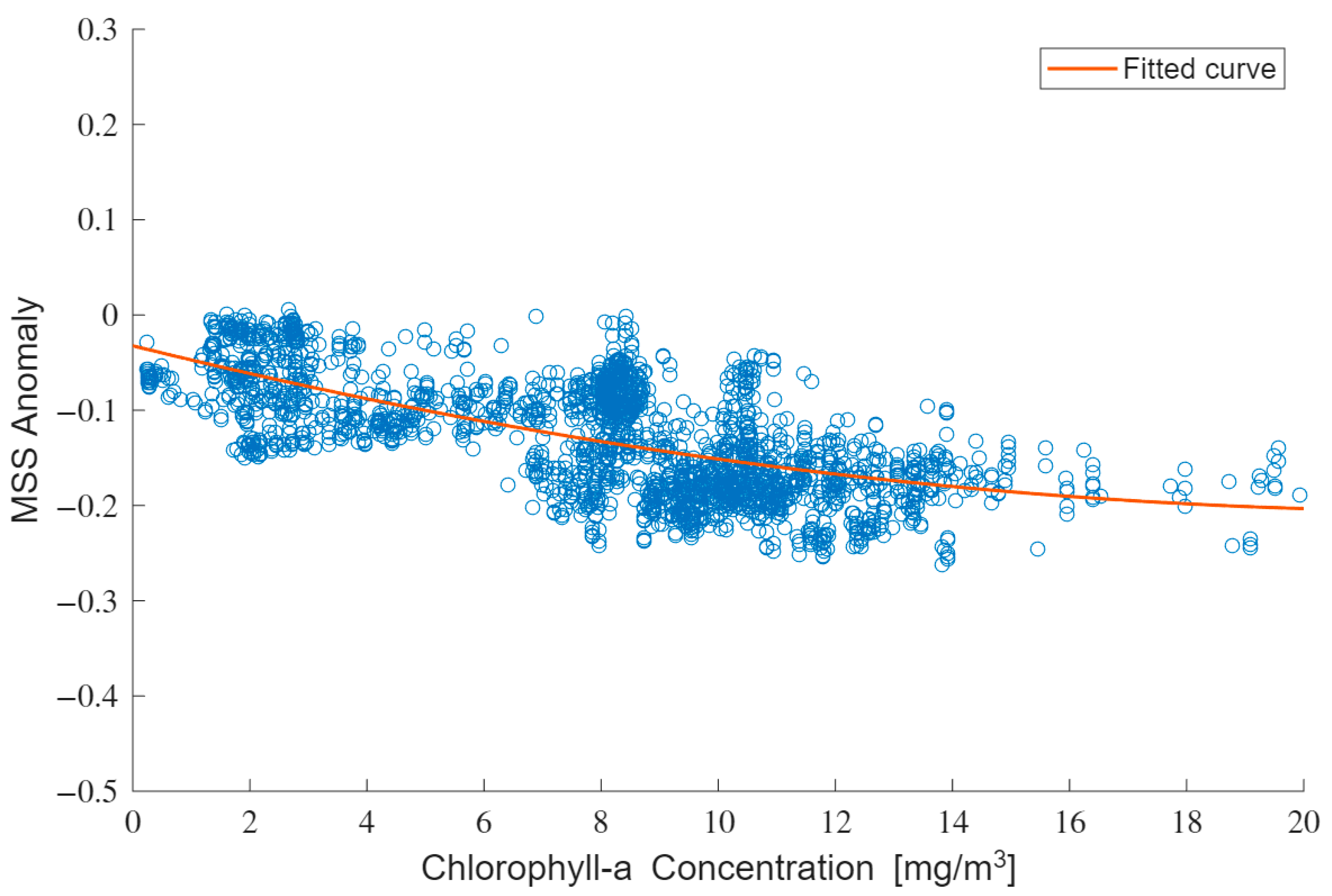
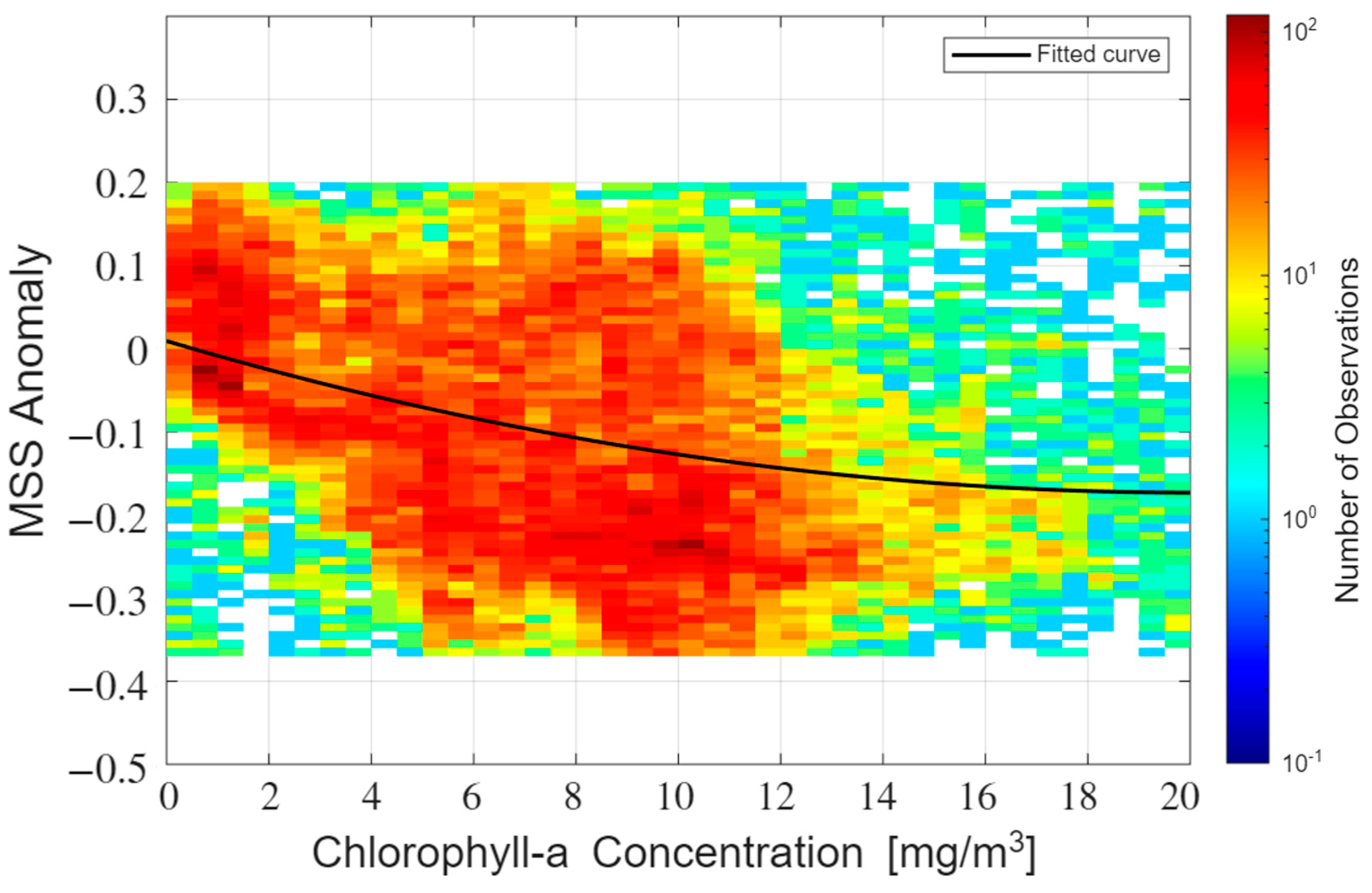
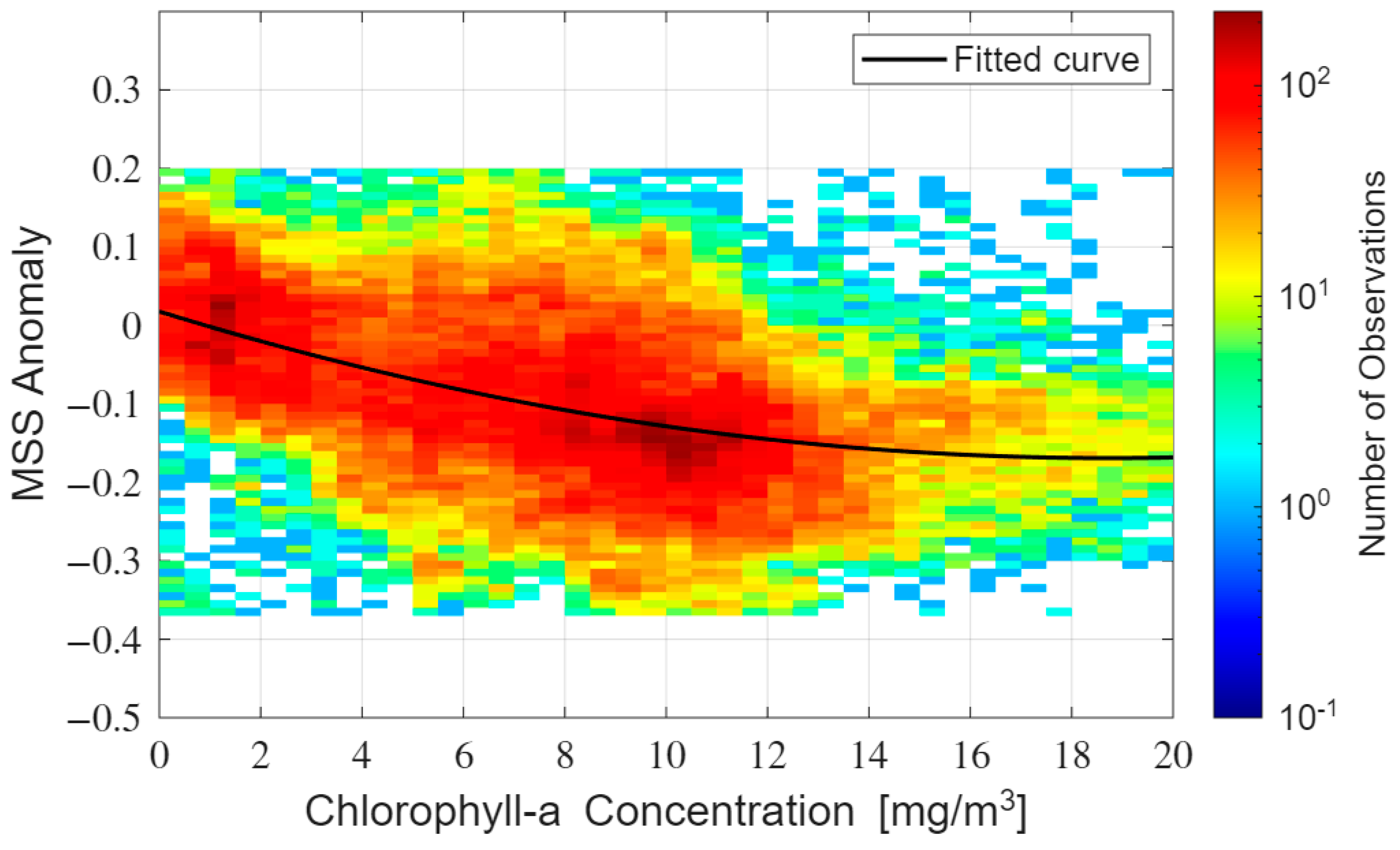
From the 35 overpasses that passed the initial filtering quality, RMSD values were calculated between the single overpass quadratic fits and the data. Using a filtering threshold of 0.1 removed some of the poorer performing outliers, and the remaining data was used to build an aggregate model. A quadratic best-fit line was fit to the aggregate model. The single overpass fits were then compared to the aggregate fit using a second RMSD filter, comparing the single overpass quadratic models to the aggregate quadratic model. This reduced the number of single overpass fits to 15. Finally, the 15 overpasses had their data aggregated, and a best-fit quadratic model was fit to the data. This data and model are plotted in Figure 11. An in-depth description of how the filtering was done can be found in Appendix B. The RMSD filtering step is a quality-control procedure for empirical model construction and should not be interpreted as independent validation. This step preferentially retains overpasses in which the hypothesized MSS anomaly–chlorophyll-a relationship is clearly expressed, and therefore the resulting model may not generalize to all coastal scenes or all bloom conditions. Independent overpasses not used in fitting are therefore evaluated separately, and the model is described as a proof-of-concept empirical retrieval rather than a globally validated chlorophyll-a product.
The Equation for the SWOT MSSANOM-Algae Model is
M S S A N O M = 4.5 × 10 4 C C 2 0.0181 C C + 0.0093 ,
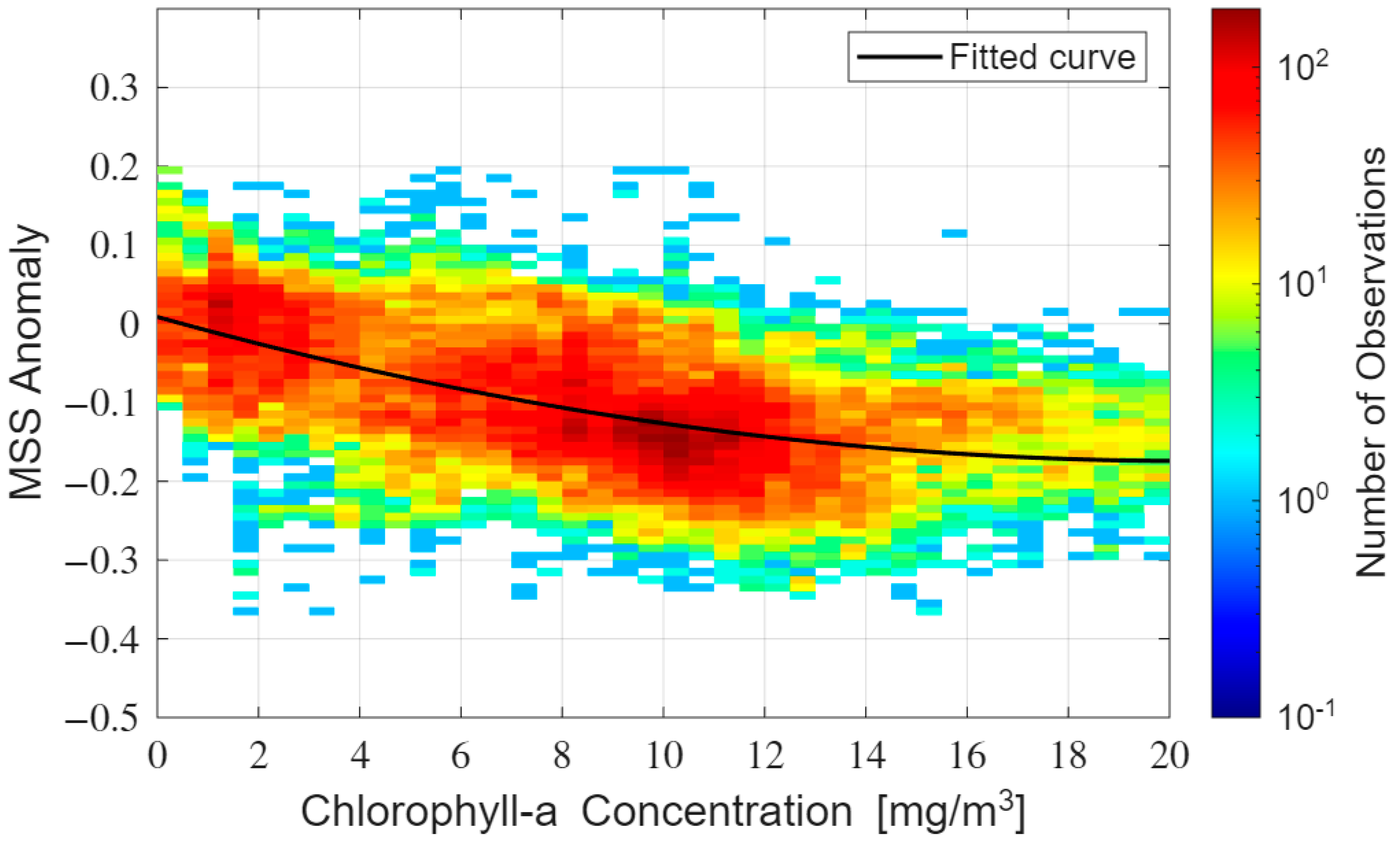
The RMSD of the aggregate fit drops from 0.0941 to 0.0660. Finally, it is important to compare the model to some of the data that was not used to train the model. Figure 12 is a comparison of the MSSANOM-Algae Model to the 20 overpasses that met the original criteria but were not used in the training set. The 20 overpasses are in a similar seasonality to the training overpasses. The operational use of the model is to retrieve chlorophyll-a concentration from an observed MSSANOM, but the model in Equation (7) is fit in the other direction. This is to match the training data structure shown in Figure 10 and Figure 11. In practice, Equation (7) must be inverted to retrieve chlorophyll-a.
The RMSD for the test data against the fit is 0.13. As Figure 12 shows, much of the data is more spread out around the model. The model captures an area of high density in the low chlorophyll regime, but as the chlorophyll goes above 6 mg/m3, the model has a harder time capturing the dynamics of the chlorophyll. Part of the increase in magnitude in MSSANOM with the increase in chlorophyll may be due to other contaminants that may be suppressing the ocean surface that are not related to chlorophyll.

3.3. Uncertainty in the Chlorophyll-A Concentration

To quantify how uncertainty in the ERA5 wind speed forcing propagates through to the final chlorophyll retrieval, we performed a Monte Carlo uncertainty analysis. Using a representative ERA5 wind speed RMS error of 1 m/s over the open ocean, we generated an ensemble of 1000 perturbed wind speed realizations for each matchup point, drawn from a normal distribution centered on the reported ERA5 wind speed with this RMS error as the standard deviation. Each perturbed wind speed was propagated through the empirical MSSmod(CT) relationship (Equation (4)) to generate an ensemble of MSSmod values, which were then used to compute a corresponding ensemble of MSS Anomaly values (Equation (5)). This MSS Anomaly ensemble was subsequently propagated through the inverse of the quadratic MSSANOM-Chlorophyll-a relationship (Equation (7)) to yield an ensemble of retrieved chlorophyll concentrations for each point. The spread of this ensemble represents the uncertainty in the final CC retrieval attributable solely to ERA5 wind speed error. Averaged across the training dataset, this analysis yields a chlorophyll concentration uncertainty of approximately 3.7 mg/m3.

3.4. Histograms of the Chlorophyll-A Concentration

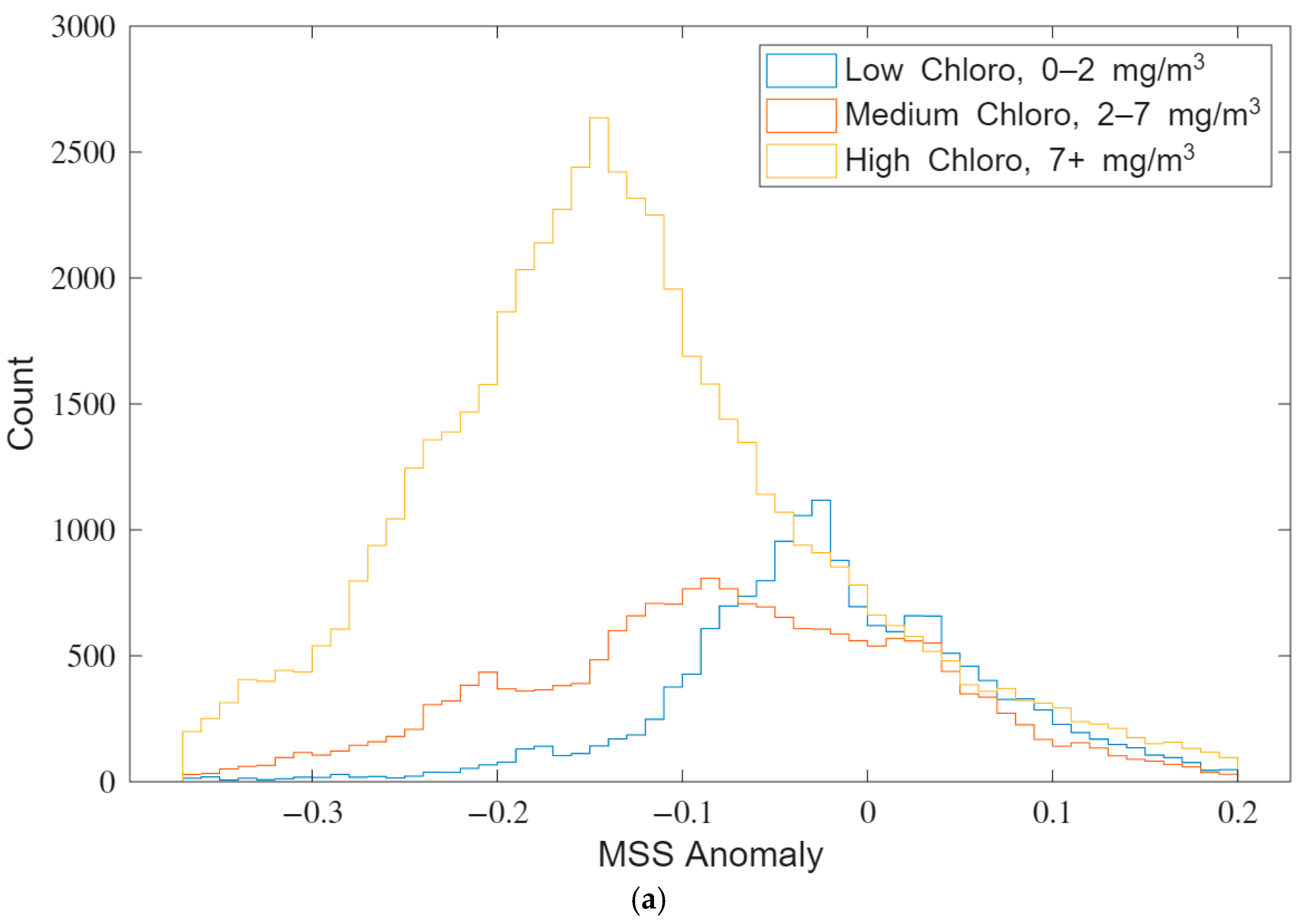
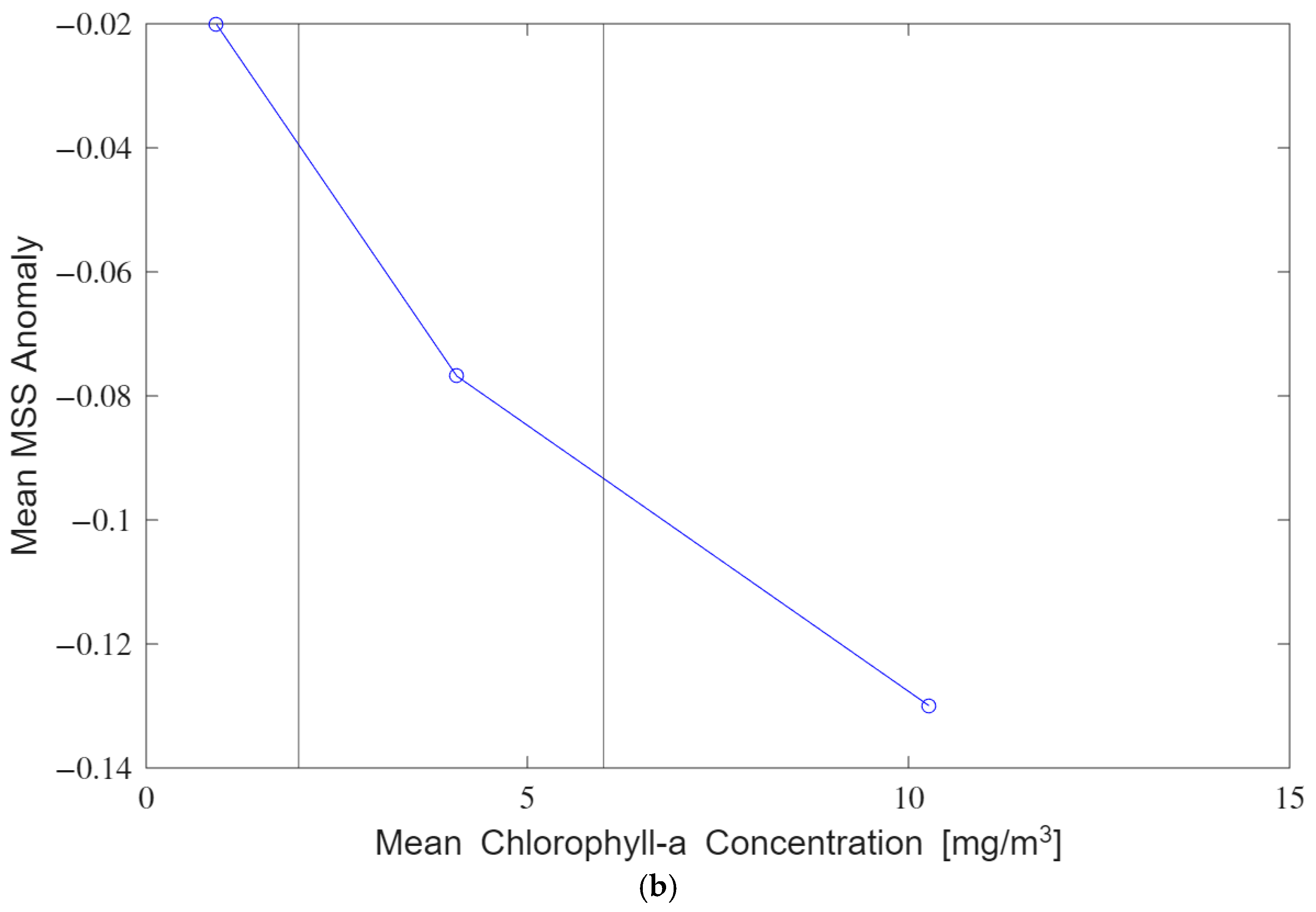
To investigate the relationship between the MSS Anomaly and varying chlorophyll concentrations in the ocean, chlorophyll data were divided into three distinct ranges: low, medium, and high concentrations. Figure 13a is a histogram used to visualize the distribution of chlorophyll values across these categories. Figure 13b is a line plot that shows the mean values of both chlorophyll and MSS Anomaly calculated within each concentration range.
As demonstrated in Figure 13, an increase in chlorophyll-a concentration pairs with a decrease in the mean MSS Anomaly, which falls from 0.04 to −0.12 across the data range.
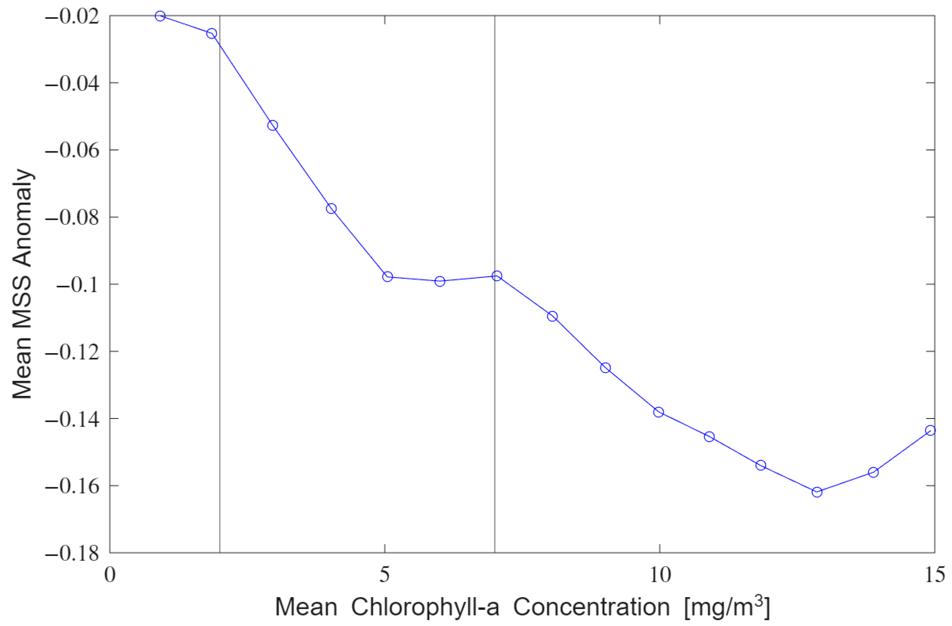
Notably, the trend persists when chlorophyll-a is binned into smaller, overlapping ranges (e.g., 0–2, 1–3 mg/m3), confirming the robustness of the relationship between chlorophyll-a concentration and MSS Anomaly across approaches. This case is displayed in Figure 14.
The drop-off in Figure 14 slows as the concentration increases, further bolstering the quadratic relationship used in our model. The tail turning up at the end of the curve is due to both lower amounts of data in the bin, and due to overall variance.

4. Results

4.1. Validation of Retrieval Algorithm

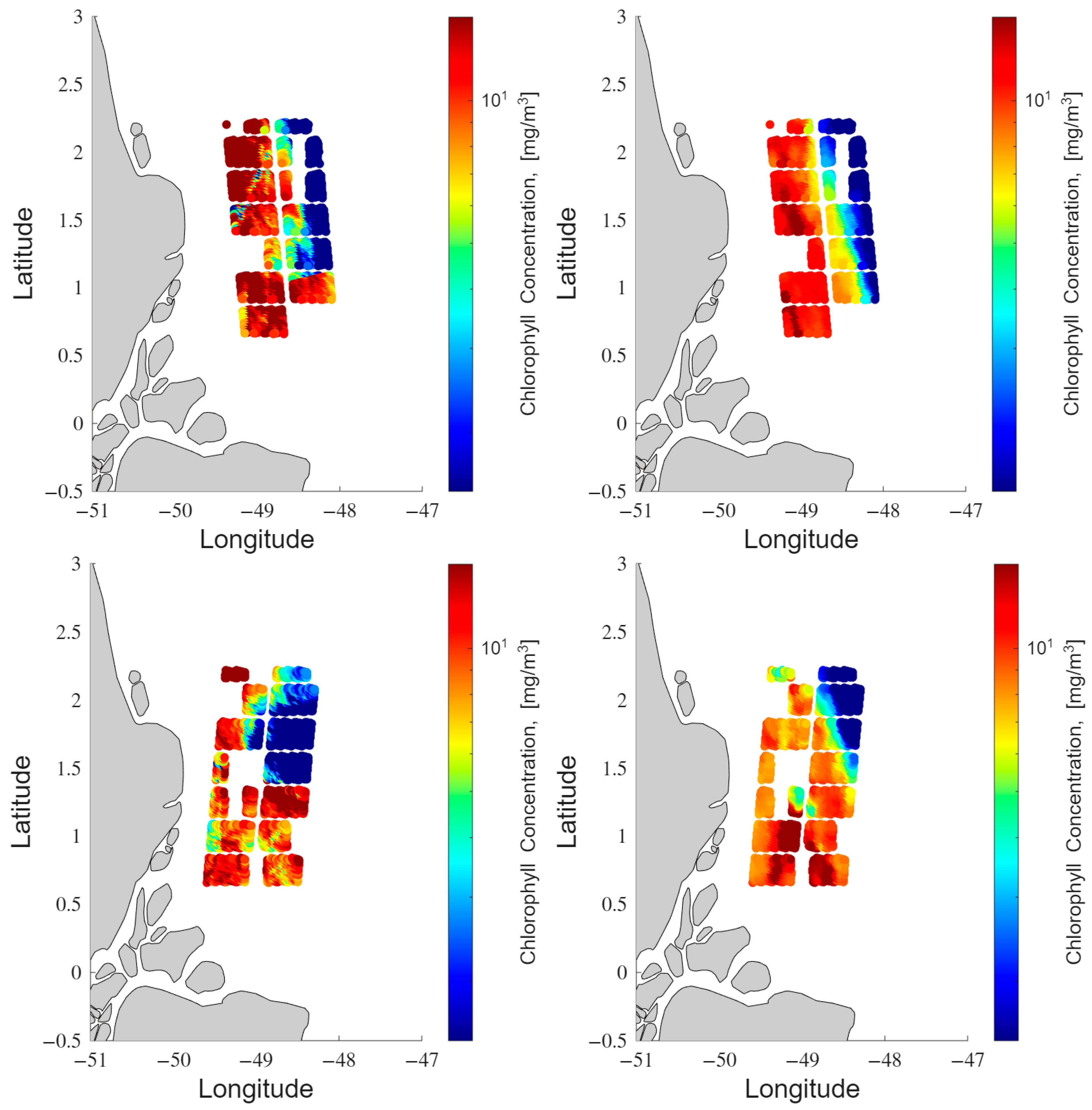
The SWOT algal bloom product is first validated by comparison to the VIIRS Gap-filled Product during the overpasses used for training the retrieval algorithm. The SWOT retrieval algorithm trained using 15 overpasses from 2024, and Figure 15 is an example of the SWOT chlorophyll-a product and the VIIRS chlorophyll-a product side-by-side.
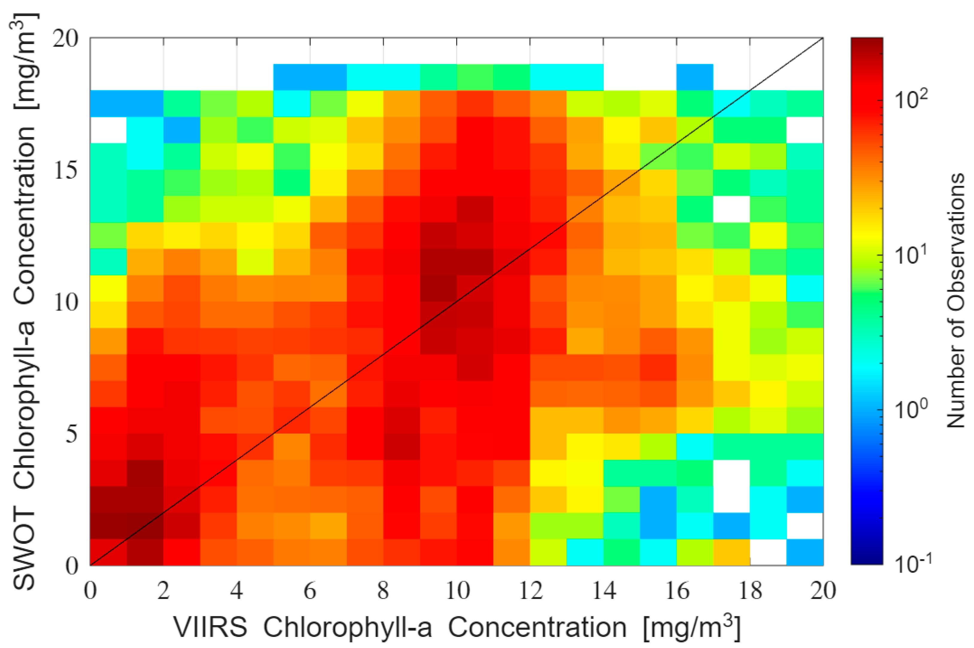
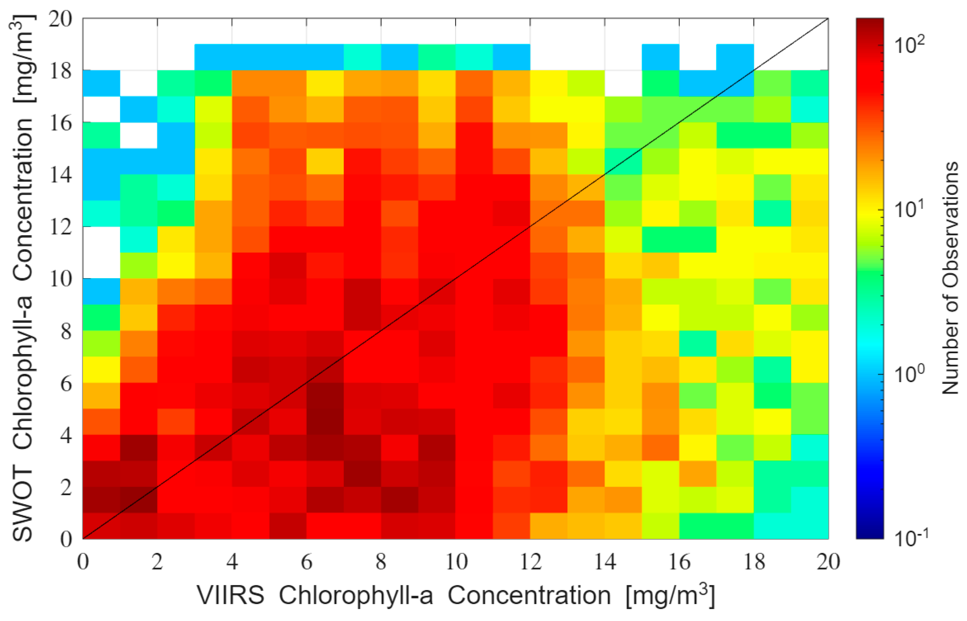
Both overpasses show that the SWOT chlorophyll-a product follows the general trend of the VIIRS product. To get an overarching view of the product, Figure 16 is a density scatter plot comparing each SWOT and VIIRS pixel 1-to-1.
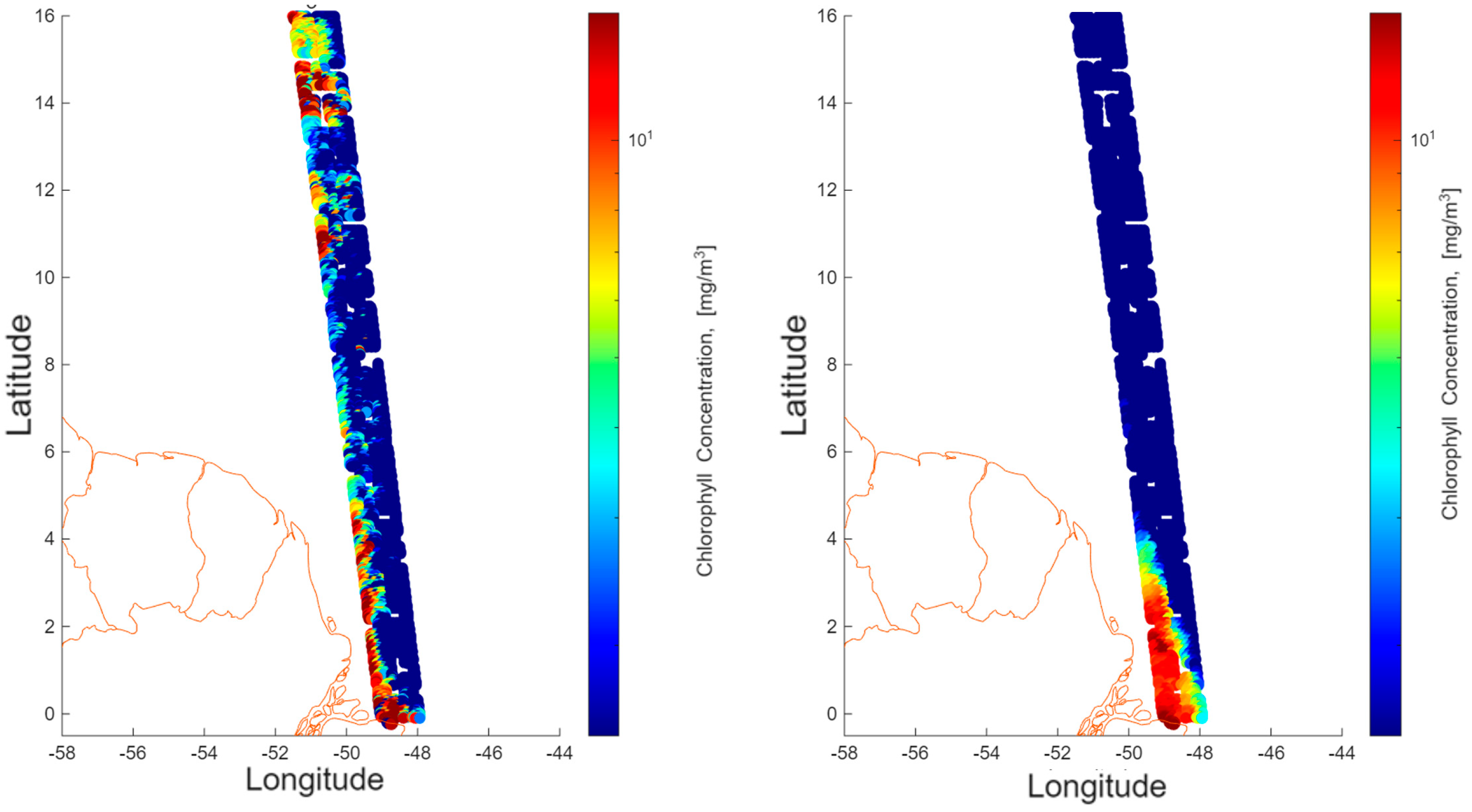
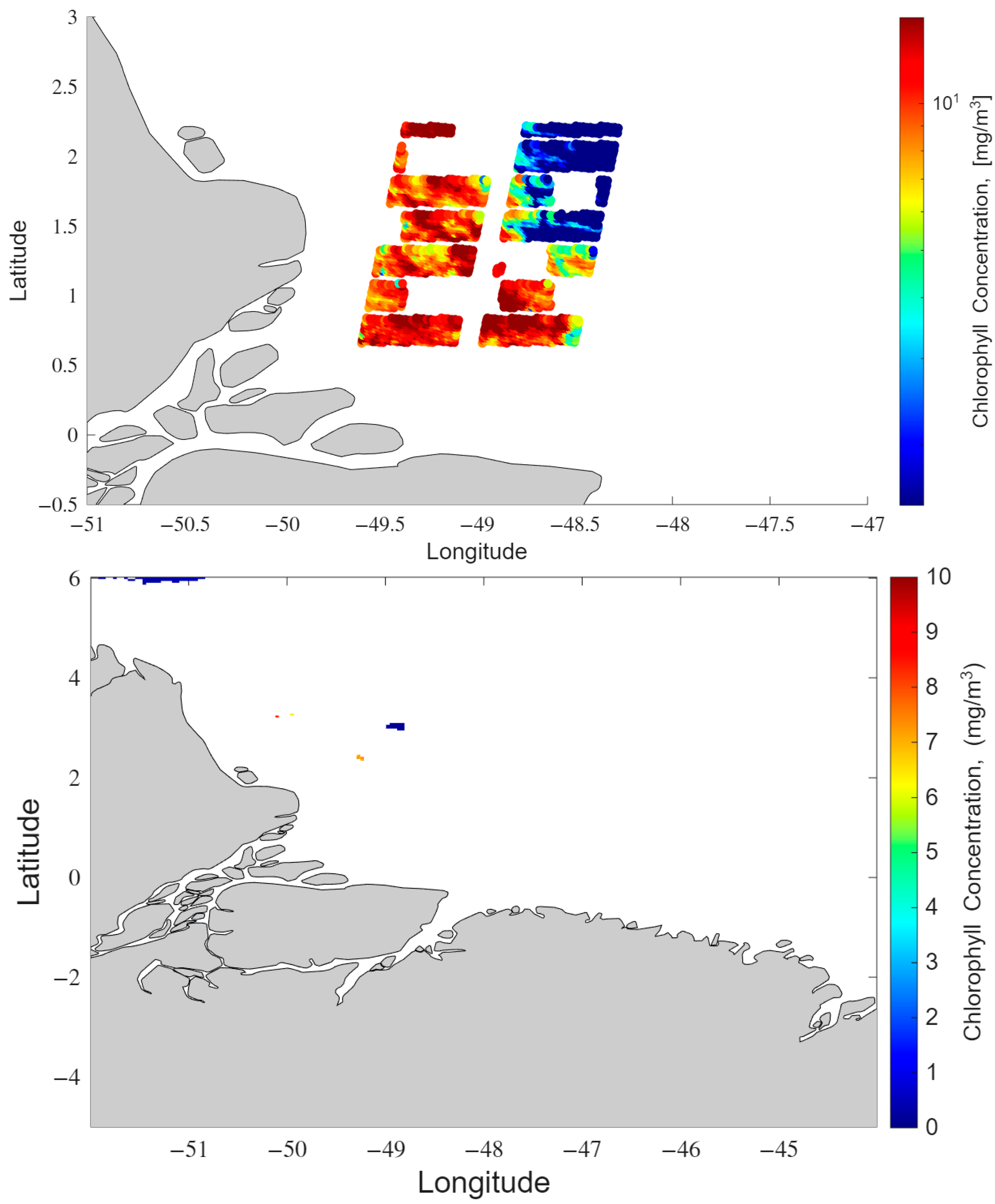
The highest density portion of the data in Figure 16 generally follows the 1-to-1 line, but with some scatter at lower densities. Figure 16 shows the results using data in the training region only. Figure 17 considers data from a full overpass on one of the training days, including samples in the Atlantic Ocean far from the training region.
As expected, VIIRS drops to near-zero values when away from coastlines. Most of the SWOT data also drops to near-zero values but does show spikes of high CC in some areas where VIIRS does not have it.

4.2. Demonstration of Retrieval Algorithm

To evaluate the performance of the retrieval algorithm outside of the training period, it is applied to independent data acquired at different times and locations. The retrieval algorithm is first applied to Amazon River data in the same region as the training data but on different days, as well as in nearby open ocean regions that were not included in the training dataset and where the retrieved chlorophyll concentration is expected to be low. The retrieval algorithm is also applied to data near the Congo River. This region represents an independent river-plume environment and retrieval results here will test the robustness of the algorithm, specifically whether there is a similar relationship between chlorophyll concentration and MSS anomaly as was observed in the Amazon training region.

Amazon River Test Cases

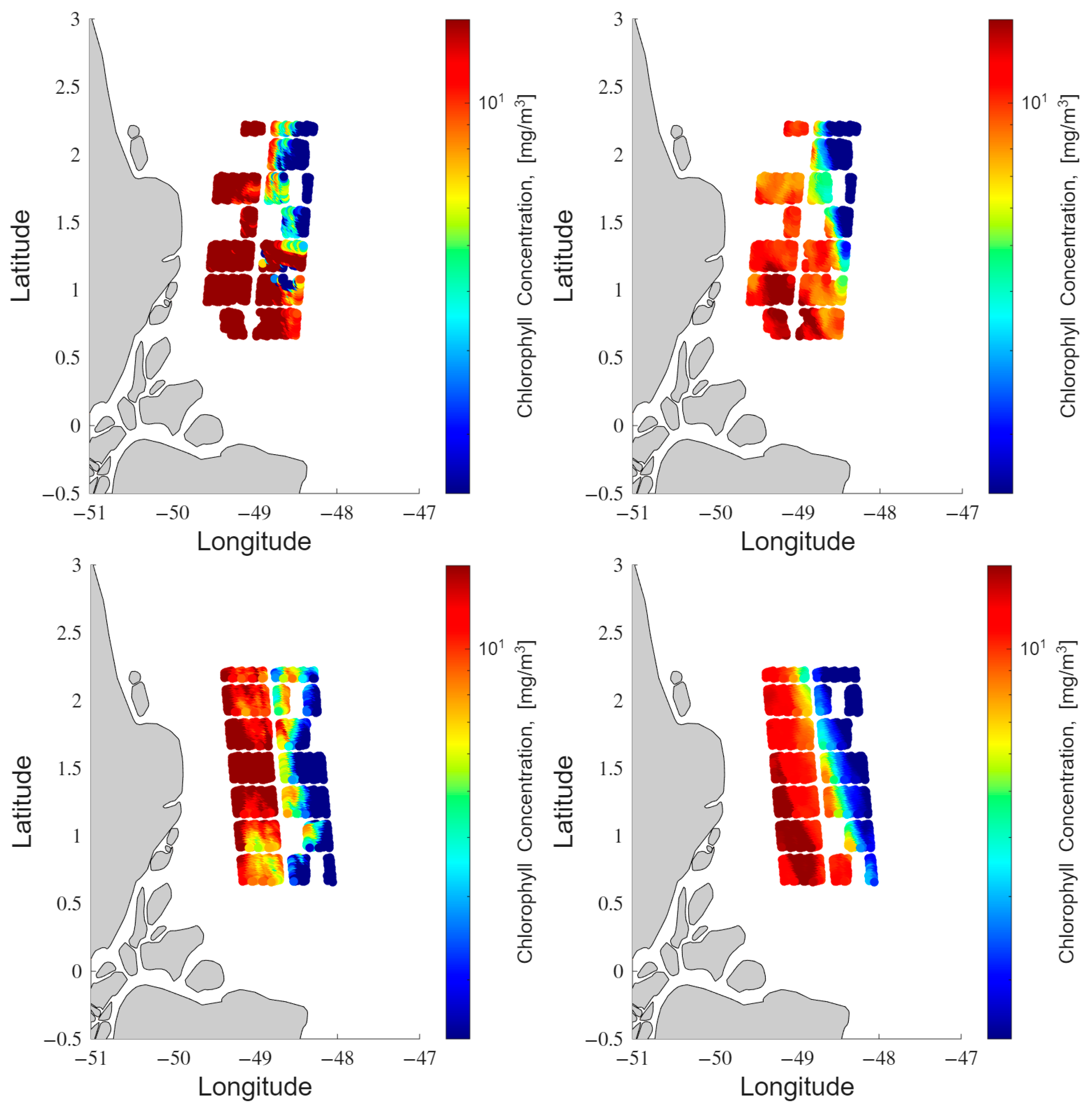
Figure 18 below is a comparison of SWOT and VIIRS CC in the testing region on two different (non-training) days.
Comparing the SWOT and VIIRS results for these two overpasses, there is general qualitative agreement. The boundary where the chlorophyll-a concentration drops off away from the coast generally agree for both overpasses, as does the shift in the boundary between passes. Like the training dataset, a density scatter plot is made of the SWOT vs. VIIRS data during the testing data days.
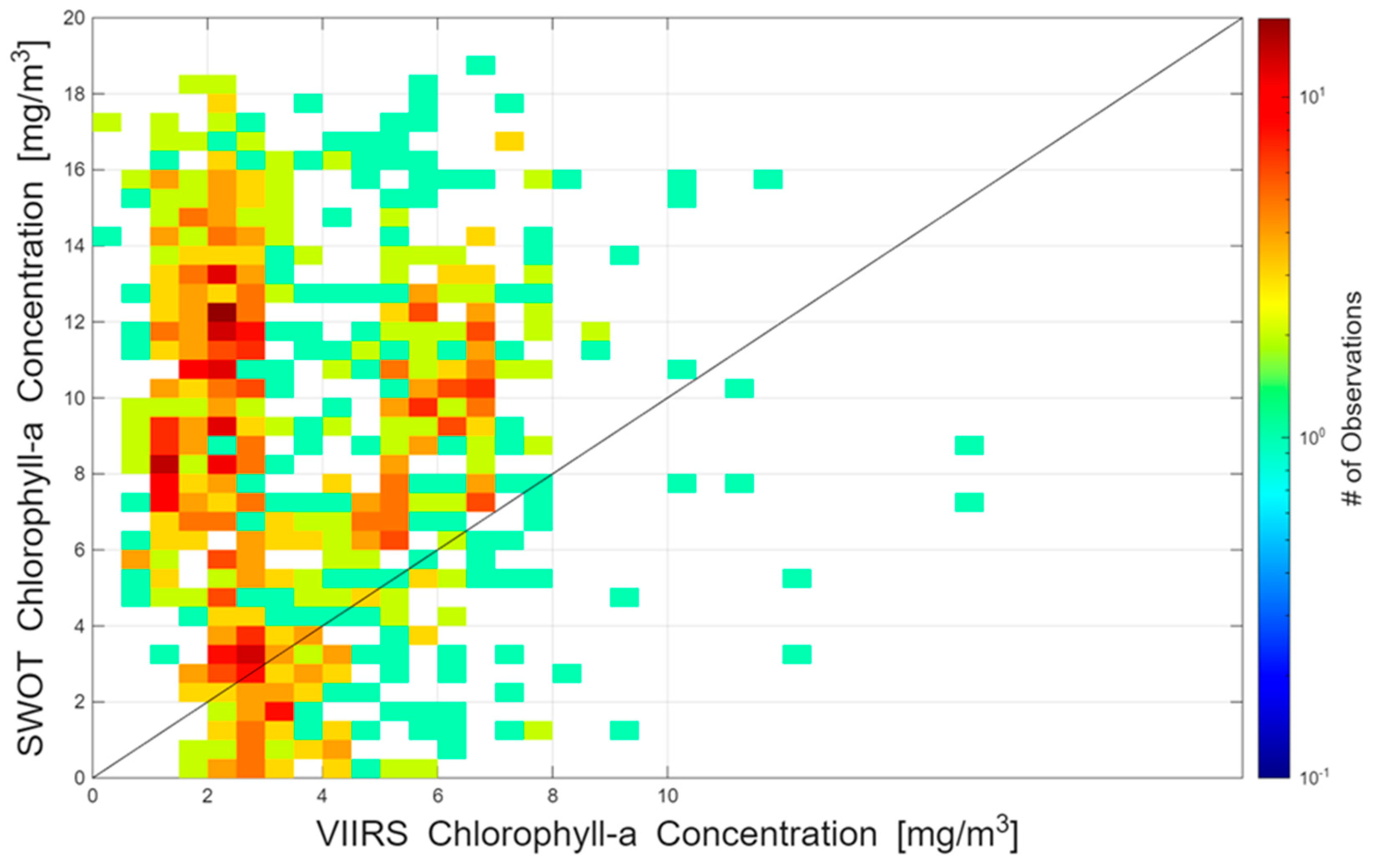
Figure 19 shows that while the comparison between SWOT and VIIRS are not perfect, there is some correlation between the two, especially at lower values of chlorophyll.

4.3. Gap-Filling of SWOT vs. VIIRS

The SWOT algal bloom product is trained on a model that uses gap-filled chlorophyll-a data to help train this model. The gap-filled data methodology involves merging different products into one product. For the VIIRS product used to train the SWOT algal bloom model, it is a combination of data from the VIIRS instrument located on the Suomi National Polar-orbiting Partnership (SNPP) satellite, VIIRS on the NOAA-20 satellite and the Ocean and Land Color Instrument (OLCI) on Sentinel-3A [26]. OLCI has a similar design to VIIRS, except it has a finer resolution and one less spectral band (21 vs. 22). Because of OLCI’s band choices, it performs better closer to the coastlines. Once these three are merged, there is calibration done to ensure OLCI and VIIRS data are gridded to the same resolution. Blank pixels are then filled in using Data Interpolating Empirical Orthogonal Functions (DINEOF). DINEOF is an iterative statistical technique, which initializes missing data with the mean value, and then uses spatial and temporal patterns to reconstruct missing values based on spatiotemporal coherence [27].
On its own, however, the daily non-gap-filled VIIRS product loses a lot of information from cloud cover. To show some of the coverage potential of SWOT, Figure 20 is a day where the SWOT data is present, and the daily coverage of VIIRS is obscured.

5. Discussion

5.1. Distinguishing Sources of MSS Anomaly

The SWOT-based algal bloom algorithm captures general features of the algal bloom distribution as shown by hyperspectral imagers. The spatial resolution of SWOT also enables a clearer depiction of coastal dynamics that are often smoothed out in coarser satellite products. This improves the ability to resolve finer scale structure in the algal bloom distribution.
However, the SWOT retrieval is fundamentally sensitive to roughness suppression rather than algal biomass directly. As a result, the algorithm flags any process that dampens short (gravity-capillary) wave surface roughness, producing false positives when interpreted as blooms. Common non-algal bloom drivers of roughness suppression include surfactant compounds unrelated to phytoplankton (natural or anthropogenic), oil or ship discharges and rain-induced damping. All these events can suppress short waves and produce negative MSSANOM.
Throughout this project, algal blooms are used as an example of a pollutant that may be detectable using a SWOT MSS and MSS Anomaly methodology, along with a secondary source of information, in our case, the VIIRS gap-filled chlorophyll-a product. Algal blooms are expected to be a dominating factor in warm, coastal, temperate conditions, but this is not expected to be a dominating force in the open ocean or in regions with colder water temperatures.

5.2. Applicability of the Amazon River Empirical Model to Other Locations

According to the VIIRS gap-filled chlorophyll-a measurements, background levels of chlorophyll-a in the Amazon River basin are around 5 mg/m3. This is a significantly higher chlorophyll-a concentration than other river mouths that were observed using VIIRS data.
Some of the above results show regions of strong suppression and high retrieved concentration which do not co-locate with elevated VIIRS chlorophyll (or other ocean-color indicators), suggesting that some of the signal likely reflects these other suppression mechanisms.
This is particularly evident near areas like the Congo River. Figure 21 looks at all the data from the Congo River, in a similar fashion to Figure 16 and Figure 19.
SWOT systematically overestimates chlorophyll-a concentration in the Congo River. The Congo River on average has a much larger negative MSS Anomaly than the Amazon, due to other contaminants that are discharged from the Congo River [28]. These other contaminants may also be causing MSSANOM, which would impact the SWOT radar measurements. The presence of other roughness-suppressing contaminants in the Congo River is likely causing false alarms in the SWOT CC algorithm, which may also be of use if proper secondary sources are used to help distinguish the source of marine litter desired.

5.3. Spatial Scale Mixing Between ERA5, SMAP & SWOT

Because ERA5 and SMAP are 10–15× coarser than SWOT, wind and salinity fields are effectively treated as locally constant over each SWOT swath segment, which will underrepresent sub-grid-scale wind and salinity variability. However, Appendix A’s description of the derivation of the Fresnel Reflection Coefficient demonstrates that MSS is largely insensitive to SSS variability. This mitigates the concerns due to SMAP, but the wind speed gridding issue is notable. Any real wind variability occurring on a grid-scale below ERA5 (0.2°) but above SWOT (2 km) will be resolved in the MSSobs but not accounted for in MSSmod. This is a limitation of using ERA5 as our comparative wind dataset, and for future work there is merit to using a higher-grade wind product as the baseline.

5.4. Temporal Scale of SWOT vs. Algal Bloom Cycle

SWOT’s temporal sampling is a significant limitation for algal bloom monitoring. As previously mentioned, the satellite has a 21-day repeat orbit, and it has an average revisit time of approximately 11 days. However, coastal blooms seen in the VIIRS data can intensify and dissipate on the timescale of days. Generally, algal blooms can persist from several days to several weeks depending on nutrient supply and physical transport. Therefore, the temporal resolution of SWOT may not be enough to capture the dynamics of algal bloom growth.
Compared with other microwave systems, SWOT provides finer spatial information than CYGNSS, but lower temporal sampling. Sentinel-1 SAR provides much finer spatial resolution, commonly on the order of 10–20 m, but its revisit time is generally longer than the revisit time of SWOT. SWOT provides a balance between CYGNSS and Sentinel-1, occupying a niche that has not been taken yet.
The present study does not suggest that SWOT should replace daily optical sensors or higher-revisit radar systems for event-scale bloom tracking. Its value is complementary: SWOT provides high spatial resolution roughness information that can be available in cloudy conditions. Future mission phases, extended operations, or constellations of SWOT-like instruments could improve temporal sampling, but evaluation of these concepts is beyond the scope of this project.

5.5. Future Work

The present study establishes a proof-of-concept relationship between SWOT-derived MSS Anomaly and VIIRS chlorophyll-a concentration, but, as noted in the Discussion, the retrieval is fundamentally sensitive to roughness suppression in general rather than to algal biomass specifically. Several directions follow directly from this limitation and are identified as priorities for future work.
While the VIIRS gap-filled chlorophyll-a data product is validated against in situ measurements such as NASA’s SeaBASS database and the Marine Optical Buoy (MOBY) system, a comparison of the SWOT measurements to direct in situ chlorophyll-a measurements would be a valuable and rigorous next step.
A systematic, region-by-region estimate of how often non-algal mechanisms are likely to dominate the observed roughness suppression would substantially strengthen confidence in the SWOT CC product. This could be approached using existing ancillary databases such as AIS-derived ship traffic density as a proxy for surfactant and oil discharge likelihood to characterize the relative risk of false positives across different coastal environments before the product is applied there.
It remains an open question whether the sign, magnitude, or spatial pattern of MSS Anomaly differs systematically between algal bloom suppression and suppression from oil, surfactants, or rain. Controlled wave tank experiments, such as those described in Section 2 earlier, offer a promising path to isolate the roughness response specific to algal concentration under known conditions and could be extended to directly compare against the roughness suppression signatures associated with oil films, as documented extensively in the SAR literature. Establishing whether these mechanisms are quantitatively separable would be a meaningful step toward a parsed apart retrieval, rather than a general roughness-suppression indicator. Taken together, these directions aim to move the SWOT CC product from its current state as a general-purpose indicator of surface roughness suppression that requires cautious, context-aware interpretation toward an operationally reliable complement to VIIRS chlorophyll-a retrievals, with quantified confidence in regions of mixed pollution sources.

6. Conclusions

This study presents a proof-of-concept empirical relationship between SWOT-derived MSS anomaly and VIIRS chlorophyll-a in the Amazon River plume. The retrieval demonstrates that SWOT can observe coastal surface roughness suppression patterns that are broadly associated with elevated chlorophyll-a under favorable conditions. A measure of ocean roughness (MSS) was derived from SWOT radar scattering cross section data. Deviations of the MSS from its usual value at a given wind speed (referred to as the MSS Anomaly) are derived from the SWOT data combined with ancillary ERA5 estimates of wind speed. MSS Anomaly is a measure of the suppression of wind-driven ocean surface roughening. It is attributed to the presence of marine litter on the surface. We consider algae as an example of marine litter, as detected by the VIIRS imager, and show that MSS Anomaly can be used to construct an algal bloom detection and tracking product in the Amazon River. The product is developed empirically from matchups between SWOT-derived MSS Anomaly and VIIRS-derived chlorophyll-a concentration (CC) across the outflow region of the Amazon River into the Atlantic Ocean. SWOT and VIIRS images of CC are found to generally agree in the Amazon outflow region. This model has a tested validity range of 0–6 mg/m3. The retrieval was also examined near the Congo River outflow as an illustrative case rather than as a formal validation. While relative trends in the two CC products agree near the Congo, there is a clear high bias in the SWOT version which is believed to be caused by the presence of other (non-algae) forms of roughness-suppressing materials in the region. The Congo River example therefore demonstrates both the potential and the limitation of the approach: SWOT can identify areas of anomalous roughness suppression, but ancillary information is required to distinguish algal blooms from other surface-active materials or pollutants. The uncertainty estimate associated with ERA5 wind speed quantifies only one component of the retrieval uncertainty and does not include structural or attribution uncertainty. Future work should include in situ chlorophyll-a validation, explicit false-positive analysis, and region-specific tests using ancillary observations of surfactants, oils, sediments, and floating material.

Author Contributions

Conceptualization, C.R. and G.S.; methodology, C.R. and G.S.; software, G.S.; validation, G.S. and C.R.; data curation, G.S.; writing—original draft preparation, G.S.; writing—review and editing, G.S. and C.R.; visualization, G.S.; supervision, C.R.; project administration, C.R.; funding acquisition, C.R. All authors have read and agreed to the published version of the manuscript.

Funding

This work was supported by NASA Science Mission Directorate contract NNL13AQ00C with the University of Michigan.

Data Availability Statement

All ERA5, SMAP, and SWOT datasets are available online, and are referenced to their exact locations below. The code used to process the datasets and generate the empirical SWOT chlorophyll-a retrieval will be made publicly available upon publication at https://github.com/gopalsun98.

Conflicts of Interest

The authors declare no conflicts of interest.

Abbreviations

The following abbreviations are used in this manuscript:
SWOTSurface Water and Ocean Topography
VIIRSVisible Infrared Imaging Radiometer Suite
SARSynthetic Aperture Radar
CYGNSSCyclone Global Navigation Satellite System
GNSS-RGlobal Navigation Satellite System Reflectometry
MSSMean Square Slope
ECMWFEuropean Centre for Midrange Weather Forecasting
ERA5ECMWF Reanalysis 5
SSTSea Surface Temperature
SSSSea Surface Salinity
RMSDRoot Mean Square Deviation
SNPPSuomi National Polar-orbiting Partnership
OLCIOcean Land Color Instrument
DINEOFData Interpolating Empirical Orthogonal Functions
CCChlorophyll Concentration
LUTLookup Table

Appendix A

Appendix A.1. Fresnel Reflection Coefficients

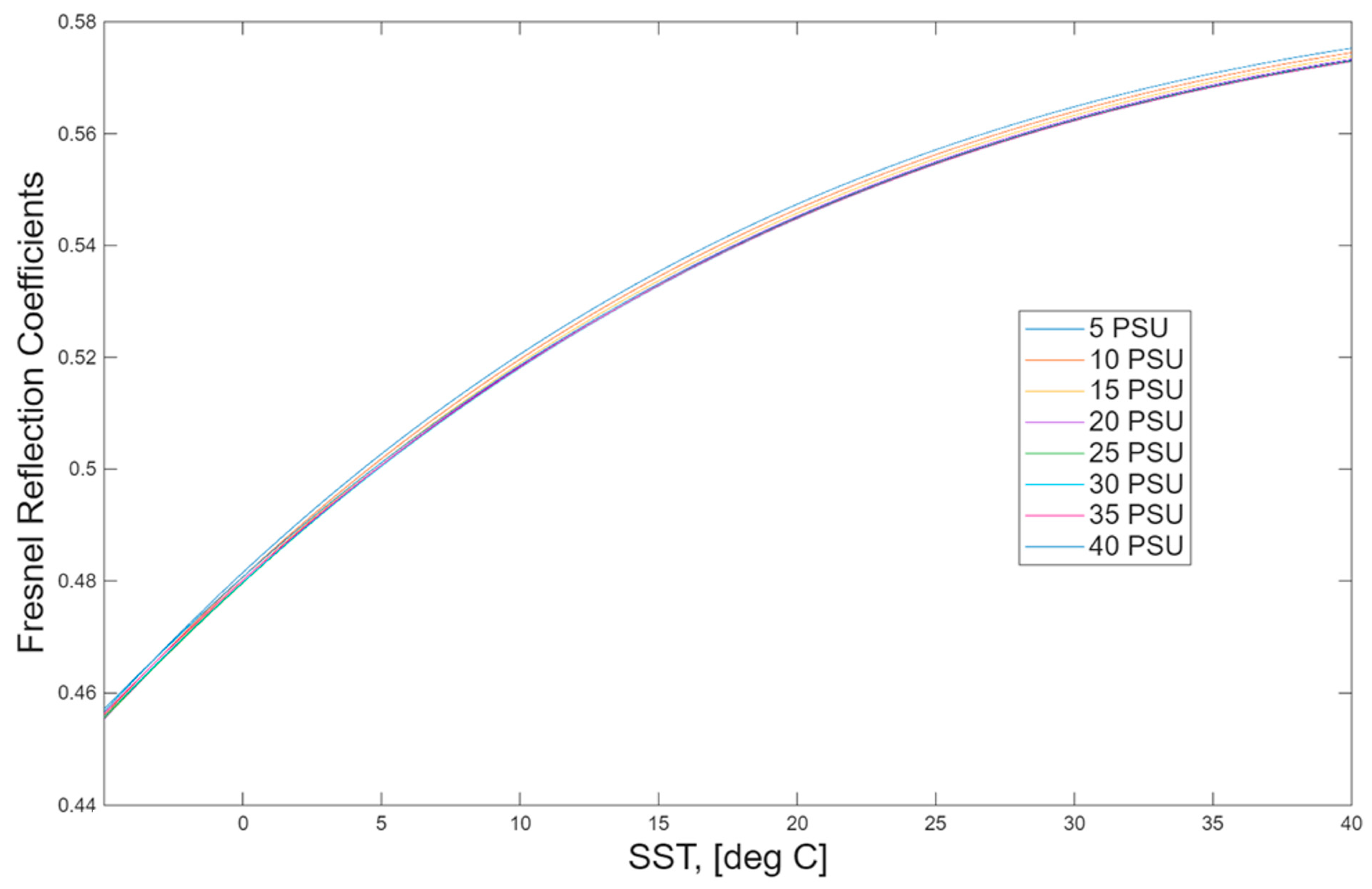
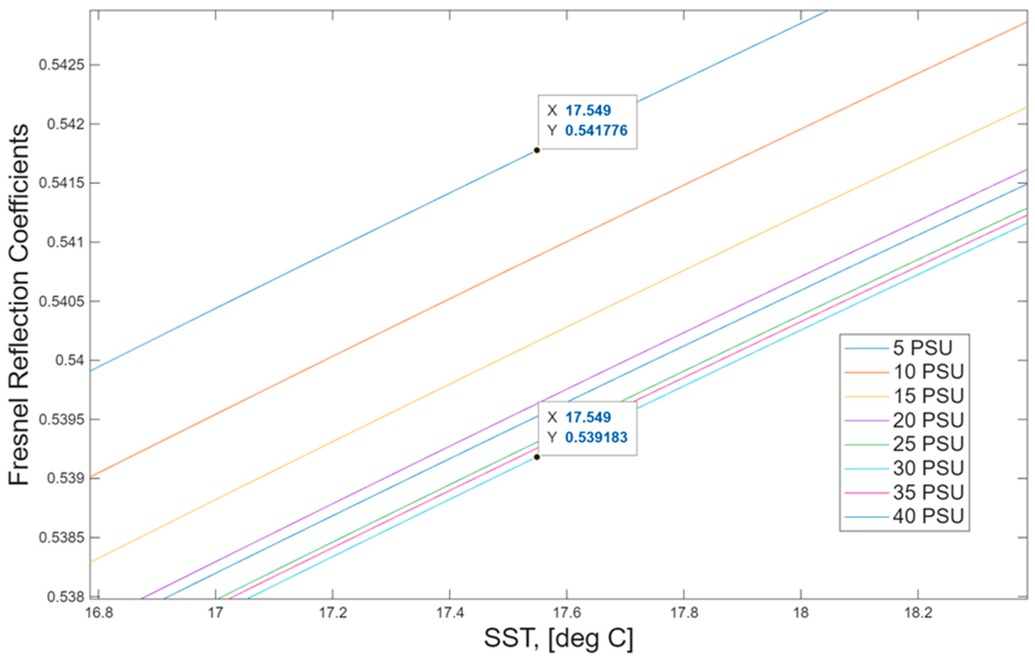
Creating the Fresnel Reflection Coefficients requires use of Equation (4), which means using ERA5 Sea Surface Temperature and SMAP Sea Surface Salinity as inputs into the Double Debye model. However, this has an incredibly computationally expensive runtime, so it was imperative to check how SST and SSS impact the Fresnel Reflection Coefficients. Figure A1 is an example of the change in Fresnel Reflection Coefficient over various SSTs, with constant SSS. Curves were plotted for multiple different salinities to check if changing salinity would impact the FR Coefficient.
Figure A1. Fresnel Coefficients over SST, showing the SSS family of curves.
Remotesensing 18 02464 g0a1
Overall, the change in FR over SST is quite minimal, but the curves start to pull apart from each other as the SST increases. Figure A2 is a zoom in on the region with the biggest difference between the curves.
Figure A2. A zoom in on the high SST region of the iso-salinity curves.
Remotesensing 18 02464 g0a2
This region has the biggest split between SSS curves, with a max difference between the top curve and bottom curve of 0.0026. Even if there is a split, it may not matter. With this range of FR Coefficients [0.455–0.57], we need to see how much the FR affects MSS, and how much the difference in FR (e.g., 0.539183 to 0.541776) will affect at a given SST will change the MSS.
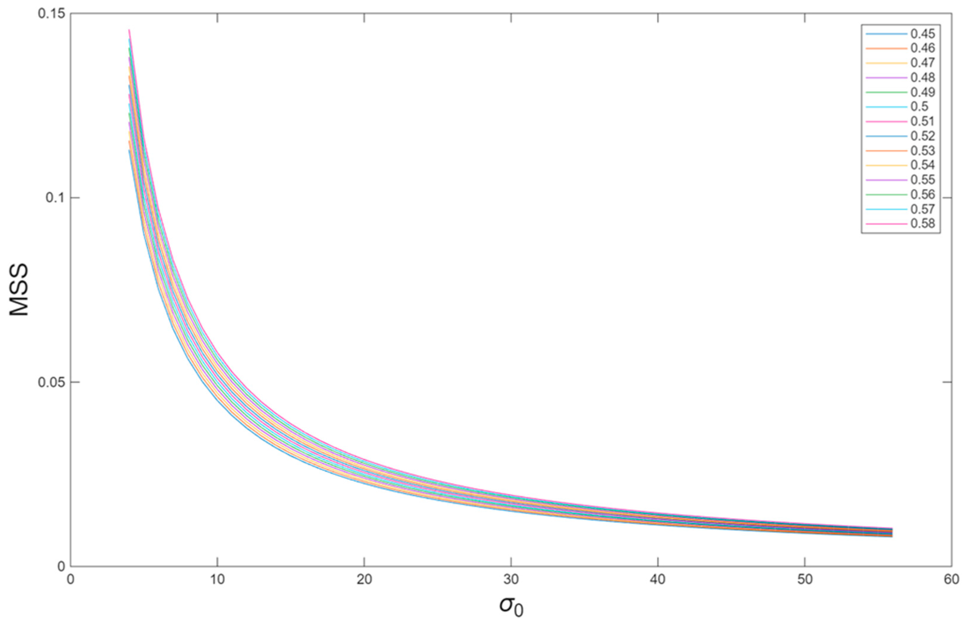
The dynamic range we are currently using for σ0 is 6–17.5 dB [29]. Converting into linear units, this means the sigma0 used is between 100.6 and 101.75. Figure A3 looks at MSS over the entire FR Coefficient range.
Figure A3. MSS over the entire range of Fresnel Coefficients.
Remotesensing 18 02464 g0a3
Because of the ~1/x relationship between sigma0 and MSS, this curve carries the shape of 1/x. This means the area where the MSS is most affected by FR is at low sigma0 values.
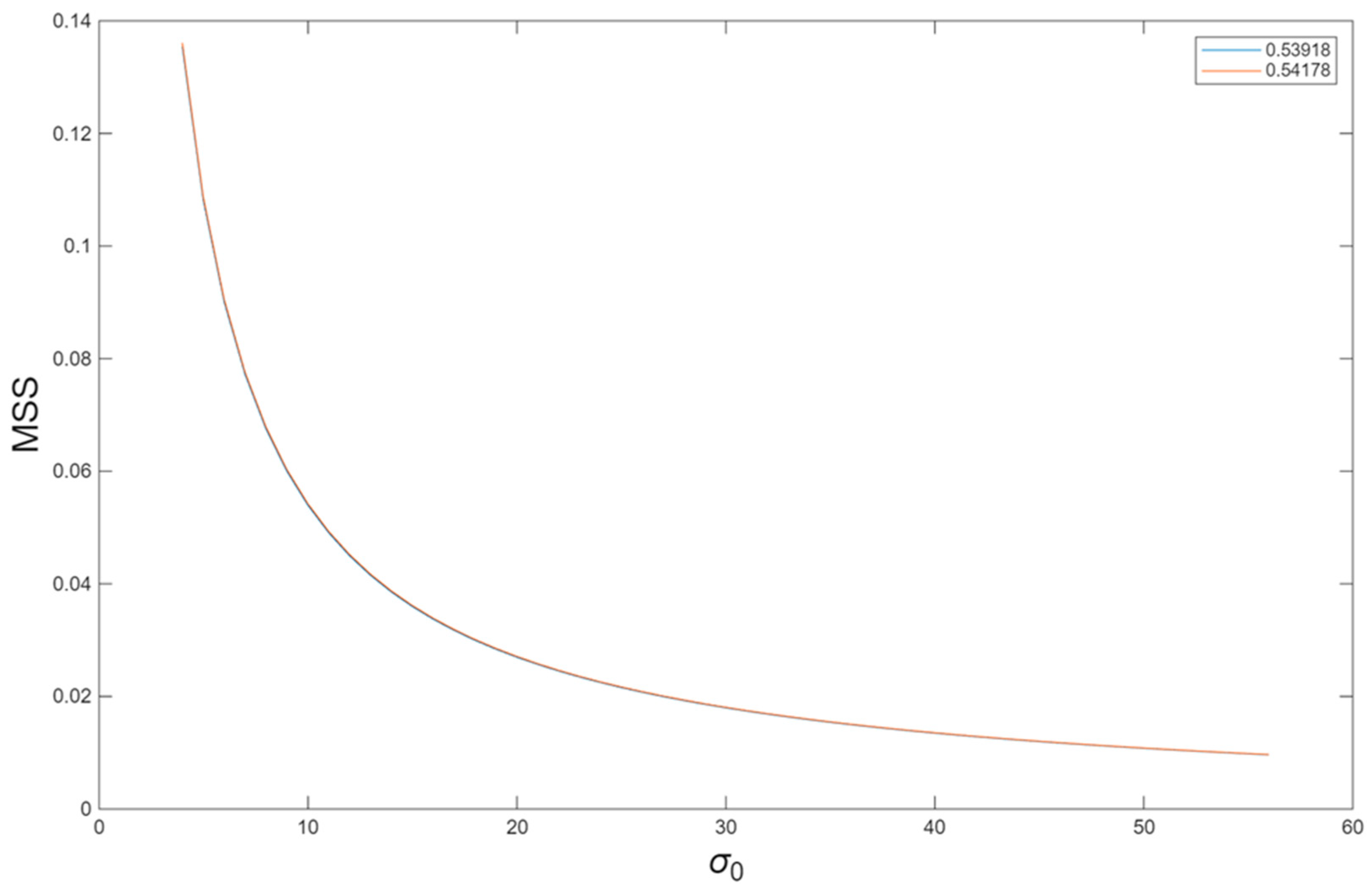
Taking two curves of FR = 0.539183 and FR = 0.541776, we can compare them and see the MSS difference along the whole curve. The two curves are plotted out in Figure A4.
Figure A4. MSS curves that have the biggest variance in FR(SST) across SSS.
Remotesensing 18 02464 g0a4
These two curves are incredibly similar. The biggest difference between these curves is 6.51 × 10⁻⁴, which is negligible. This shows that even the super low SSS does not affect the MSS.

Appendix A.2. Incidence Angle Changes

The Equation for the Fresnel Reflection Coefficients is
R ϵ ,   θ = 1 2   ϵ f , T , S cos θ ϵ sin 2 θ ϵ cos θ + ϵ sin 2 θ cos θ ϵ sin 2 θ cos θ + ϵ sin 2 θ ,
where ε(f,T,S) is the relative dielectric permittivity of seawater, which now can be determined using just frequency and temperature. The other parameter that can affect the FR Coeff is the incidence angle. Incidence angles are varied to see the FR curves over the θ family in a similar manner to SSS.
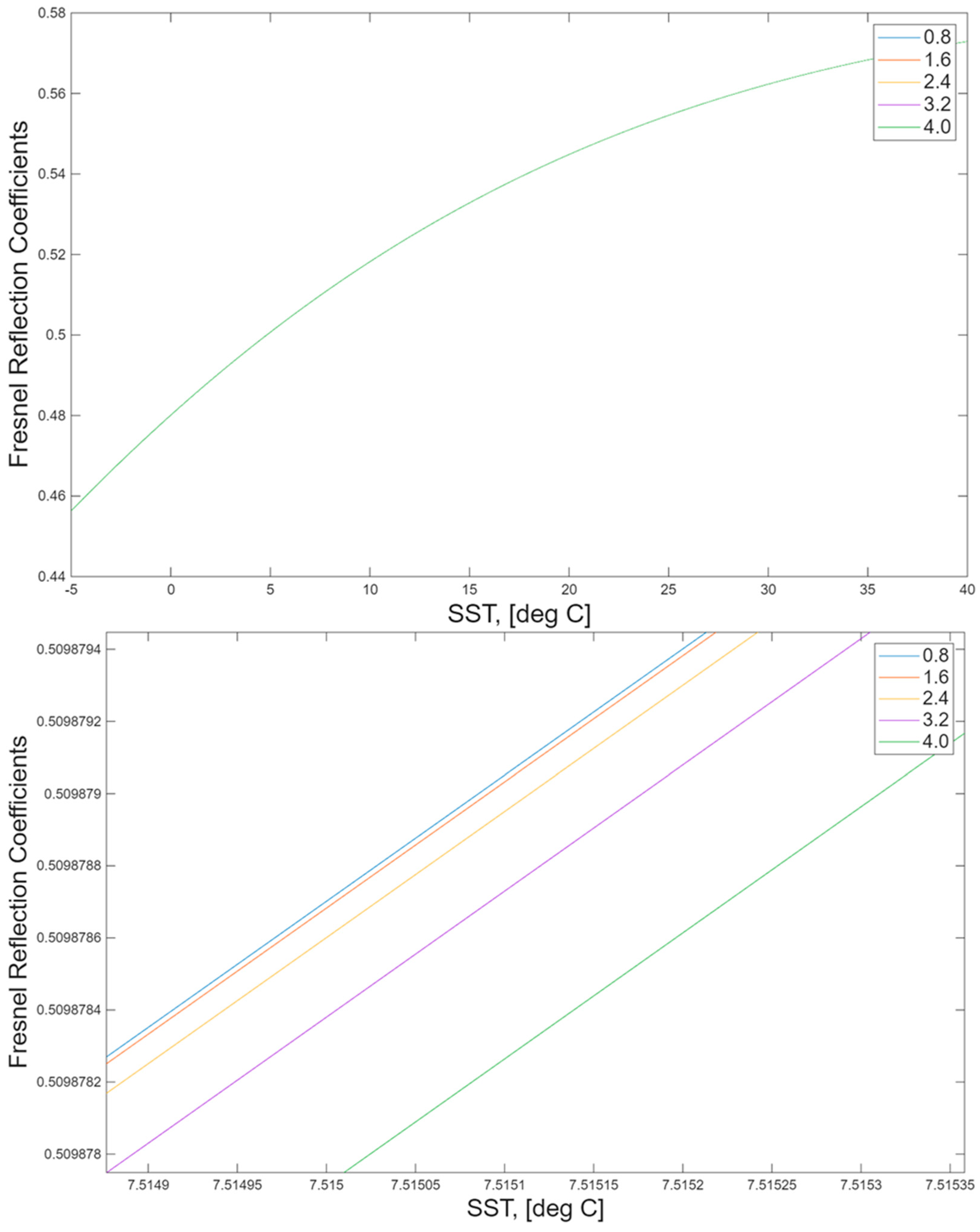
Varying the incidence angle from 0.8 to 4 degrees, Figure A5 has the family of incidence angle curves over SST.
Figure A5. (top) FR(θ) across SST for varying incidence angles. (bottom) Zoomed in version of (top) to show the difference between the family of curves.
Remotesensing 18 02464 g0a5
The change in FR for θ is significantly smaller than the one in FR for SSS. Therefore, θ in the FR Coefficient does not seem to matter. The change in MSS is orders of magnitude smaller than the FR change.
This makes Fresnel Reflection Coefficients dependent solely on sea surface temperature. To improve coding runtime and simplify the problem, a lookup table (LUT) is created for as close of a 1 to 1 matchup between FR Coeff and SST as possible.
Appendix A evaluates only the direct influence of SST, SSS, and incidence angle on the Fresnel Reflection Coefficient used in the MSS calculation. It does not quantify indirect environmental effects associated with salinity fronts, convergence, plume dynamics, or the co-accumulation of algae, surfactants, oils, or floating debris. These processes may influence surface roughness independently of chlorophyll-a and therefore represent structural sources of uncertainty in the empirical retrieval.

Appendix B

In-Depth Description of Filtering the Overpasses Further to Make the SWOT MSSANOM-Algae Model

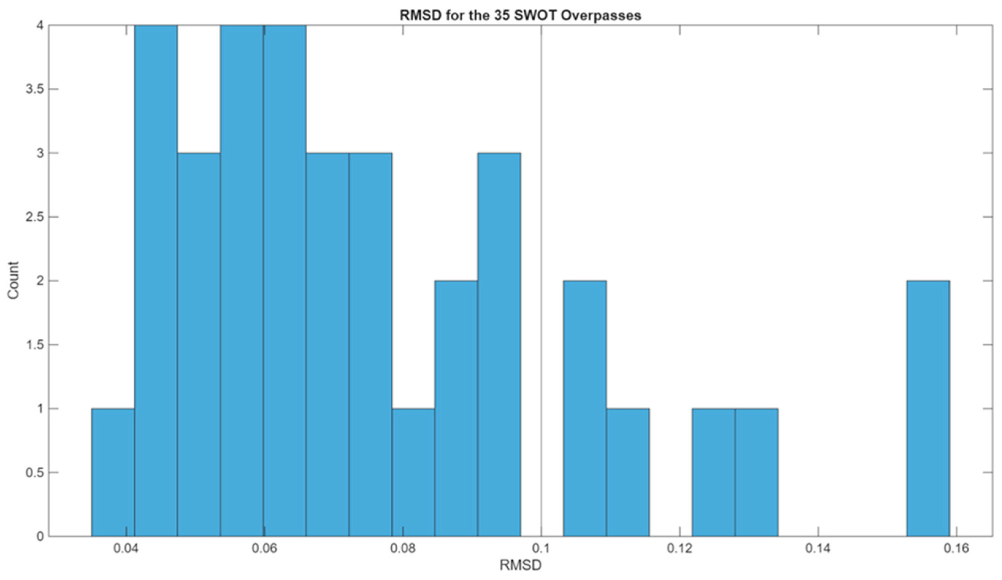
From the 35 SWOT overpasses with log fits between MSSANOM and chlorophyll-a, the RMSD was calculated for each overpass. Figure A6 displays a histogram of RMSD values.
Figure A6. A histogram of the RMSD between the logarithmic best-fit curves and the SWOT-VIIRS matched up data.
Remotesensing 18 02464 g0a6
A filtering threshold of RMSD ≤ 0.1 was used to capture the mean and mode of the data, while excluding some of the poorer outlier cases.
With this filter, 28 overpasses are now included in the model training dataset. The complete set of 28 overpasses is combined to produce a single aggregate model. Figure A7 is a scatter plot of all the MSSANOM and chlorophyll-a matchup data from the 28 overpasses, with a best-fit quadratic fit overlaid on top.
Figure A7. A scatter plot of all the SWOT and VIIRS data overlaid with a quadratic best-fit line.
Remotesensing 18 02464 g0a7
The Equation for the quadratic fit in Figure A7 is
  M S S A N O M = 5.4 10 4 C C 2 0.0201 C C + 0.0179
where MSSANOM is the MSS Anomaly predicted from CC, the chlorophyll-a concentration.
Figure A7 has an RMSD of 0.0941. This is higher than the majority of the single overpass curves, but this can be parsed apart by looking at the roll-off terms and scale factor terms of each of the single overpass curves.
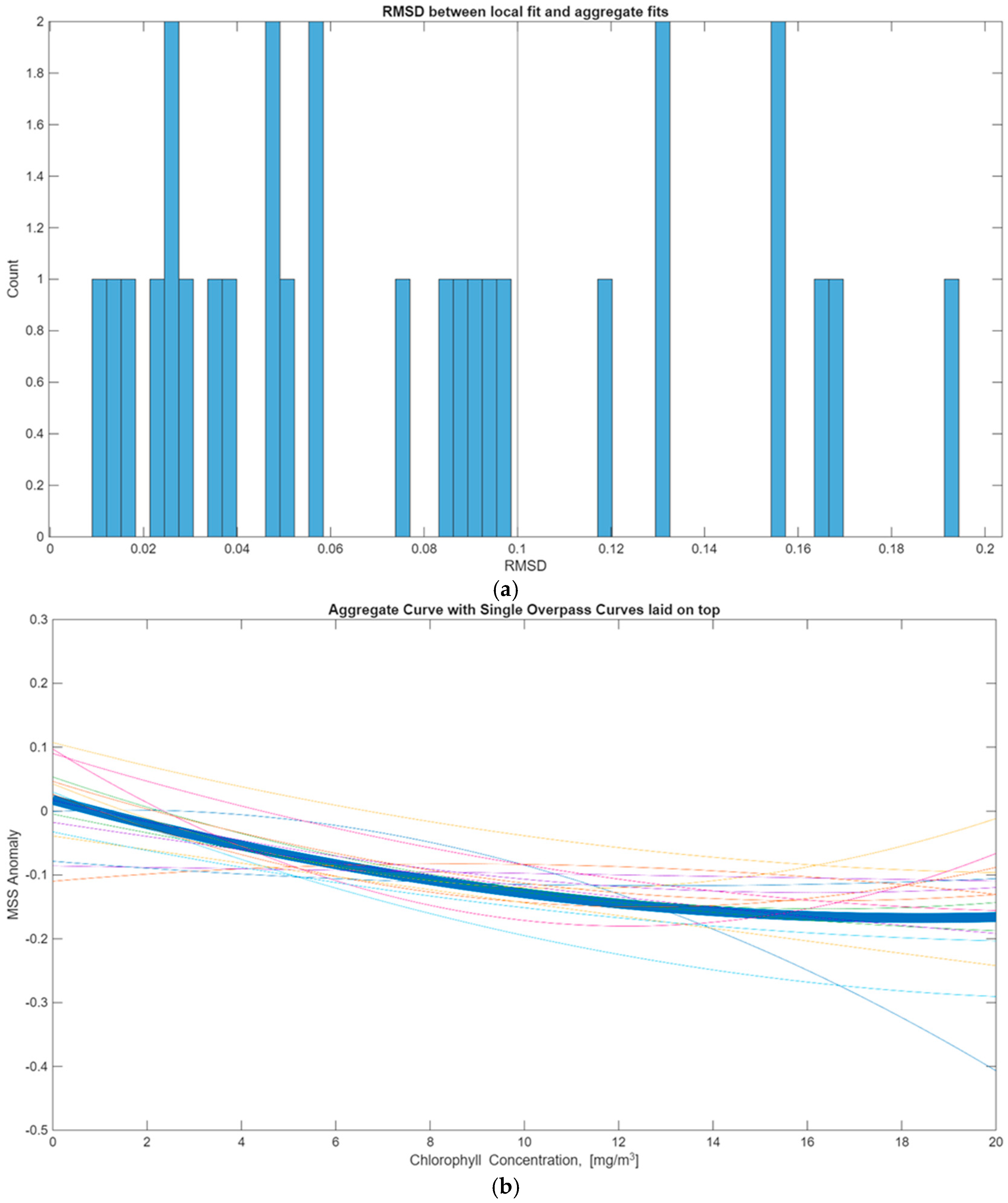
From the aggregate fit, we can compare the single overpass fits to the aggregate fit and check the RMSD between the fits. Figure A8a is a histogram of the RMSD between the single overpass fits and the aggregate fits. Figure A8b is a plot of all the single overpass fits overlaid on top of the aggregate fit.
Figure A8. (a) A histogram of the RMSD between the single overpass fits and the aggregate fit. (b) The single overpass curves are overlaid on the aggregate curve.
Remotesensing 18 02464 g0a8
Using the histogram in Figure A8a, another RMSD threshold can be established, this time at 0.1. This filters out 13 of the 28 curves, leaving us with 15 overpasses.
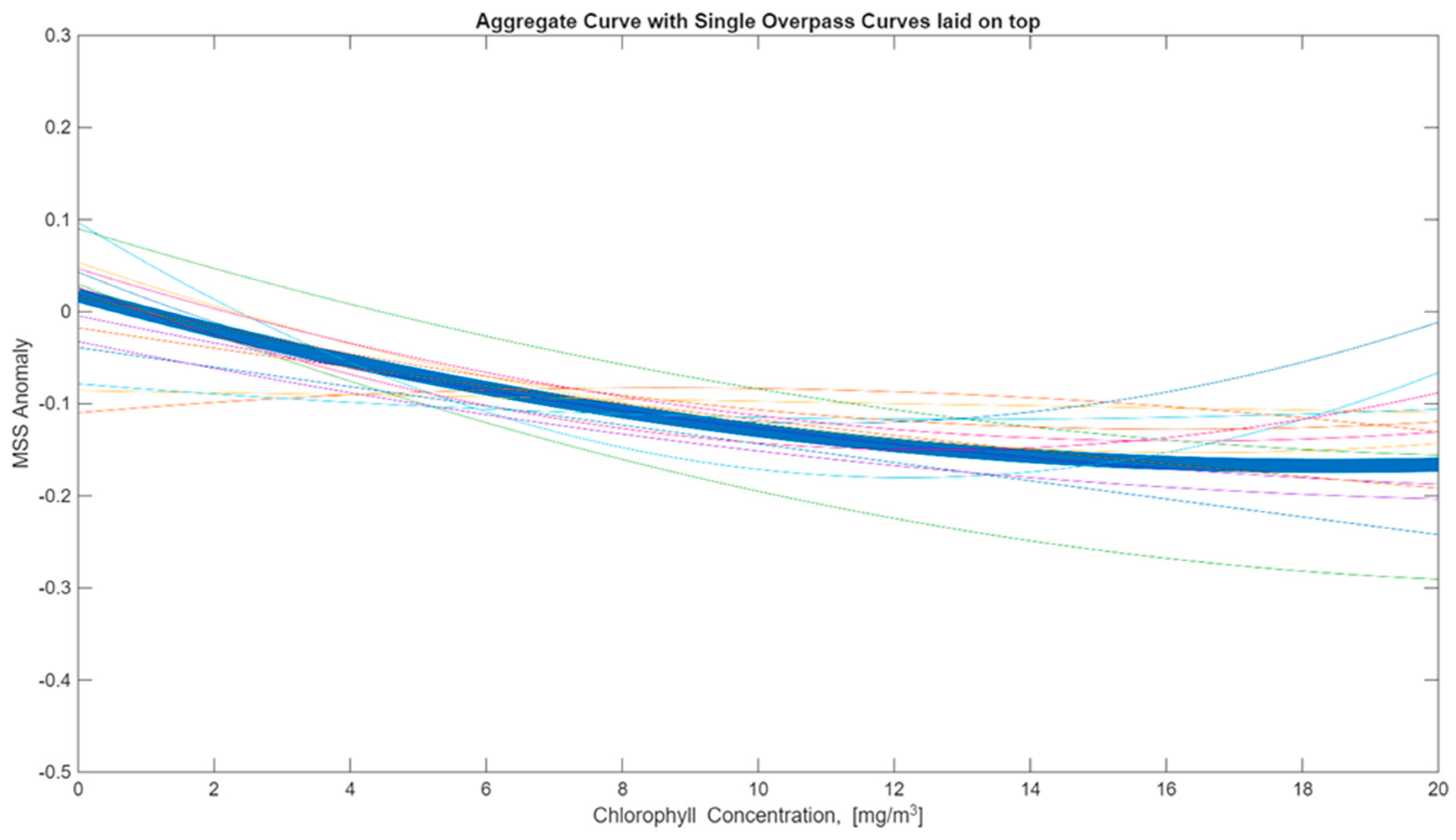
Figure A9 shows the newly filtered curves overlaid on the aggregate curve, done in the same style as Figure A8b.
Figure A9. The 15 best single overpass curves overlaid on the aggregate curve.
Remotesensing 18 02464 g0a9
From Figure A9 the process leading to Figure A7 can be repeated, as the new aggregate is plotted with a best-fit logarithmic curve, this time deciding what the SWOT MSSANOM-chlorophyll-a concentration model will look like. This is the detailed process used to derive the curve in Figure 11. Table A1 below is a description of how each filtering step reduced both the number of overpasses and pixels of data.
Table A1. Amazon River SWOT Overpass Filter.
Filtering StepOverpasses RetainedPixels Retained (Number of Points/%)
All Amazon SWOT overpasses 100 93,170, 100%
Dynamic range criteria4674,558, 80.0%
Minimum sample count4274,429, 79.8%
RMSD threshold 13563,300, 67.9%
RMSD threshold 21537,661, 40.4%
This table shows that even with only 15 overpasses in use, over 40% of the data from the Amazon is used to train the model, and 27% is used to test it.

References

  1. Wu, X.; Hou, L.; Lin, X.; Xie, Z. Application of Novel Nanomaterials for Chemo- and Biosensing of Algal Toxins in Shellfish and Water. In Novel Nanomaterials for Biomedical, Environmental and Energy Applications; Elsevier: Amsterdam, The Netherlands, 2019; pp. 353–414. [Google Scholar] [CrossRef]
  2. Hudnell, H.K. The state of U.S. freshwater harmful algal bloom assessments, policy and legislation. Toxicon 2010, 55, 1024–1034. [Google Scholar] [CrossRef] [PubMed]
  3. Lopez, C.B.; Jewett, E.B.; Dortch, Q.; Walton, B.T.; Hudnell, H.K. Scientific Assessment of Freshwater Harmful Algal Blooms; Interagency Working Group on Harmful Algal Blooms, Hypoxia, and Human Health of the Joint Subcommittee on Ocean Sciences and Technology: Washington, DC, USA, 2008. [Google Scholar]
  4. Misiou, O.; Koutsoumanis, K. Climate change and its implications for food safety and spoilage. Trends Food Sci. Technol. 2022, 126, 142–152. [Google Scholar] [CrossRef]
  5. O’Reilly, J.E.; Werdell, P.J. Chlorophyll algorithms for ocean color sensors-OC4, OC5 & OC6. Remote Sens. Environ. 2019, 229, 32–47. [Google Scholar] [PubMed]
  6. Wang, M.; Liu, X.; Jiang, L.; Son, S. The VIIRS Ocean Color Product Algorithm Theoretical Basis Document, Version 1.0; NOAA NESDIS STAR: College Park, MD, USA, 2017. [Google Scholar]
  7. Marghany, M. Utilization of a genetic algorithm for the automatic detection of oil spill from RADARSAT-2 SAR satellite data. Mar. Pollut. Bull. 2014, 89, 20–29. [Google Scholar] [CrossRef] [PubMed]
  8. Júnior, J.M.N.d.S.; de Mendonça, L.F.F.; Costa, H.d.S.; de Freitas, R.A.P.; Casagrande, F.; Lindemann, D.d.S.; Reis, R.A.D.N.; Lentini, C.A.D.; Lima, A.T.d.C. Dispersion analysis of the 2017 Persial Gulf oil spill based on remote sensing data and numerical modelling. Mar. Pollut. Bull. 2024, 205, 116639. [Google Scholar] [CrossRef]
  9. Espeseth, M.M.; Jones, C.E.; Holt, B.; Brekke, C.; Skrunes, S. Oil-spill-response-oriented information products derived from a rapid repeat time series of SAR images. IEEE J. Sel. Top. Appl. Earth Obs. Remote Sens. 2020, 13, 3448–3461. [Google Scholar] [CrossRef]
  10. Ruf, C.S.; Atlas, R.; Chang, P.S.; Clarizia, M.P.; Garrison, J.L.; Gleason, S.; Katzberg, S.J.; Jelenak, Z.; Johnson, J.T.; Majumdar, S.J.; et al. New Ocean Winds Satellite Mission to Probe Hurricanes and Tropical Convection. Bull. Am. Meteorol. Soc. 2016, 97, 385–395. [Google Scholar] [CrossRef]
  11. Hersbach, H. Sea Surface Roughness and Drag Coefficient as Functions of Neutral Wind Speed. J. Phys. Oceanogr. 2011, 41, 247–251. [Google Scholar] [CrossRef]
  12. Evans, M.C.; Ruf, C.S. Towards the Detection and Imaging of Ocean Microplastics with a Spaceborne Radar. IEEE Trans. Geosci. Remote Sens. 2022, 60, 4202709. [Google Scholar] [CrossRef]
  13. Evans, M.C.; Ruf, C.S.; Sundaram, G.B. CYGNSS Microplastic Product Version 3.2 Algorithm Theoretical Basis Document; 2024. Available online: https://podaac.jpl.nasa.gov/dataset/CYGNSS_L3_MICROPLASTIC_V3.2 (accessed on 14 January 2026).
  14. Surface Water Ocean Topography. SWOT Level 2 KaRIn Low Rate Sea Surface Height Data Product, Version D; PO.DAAC: Pasadena, CA, USA, 2025. Available online: https://www.earthdata.nasa.gov/data/catalog/pocloud-swot-l2-lr-ssh-d-d (accessed on 14 January 2026).
  15. Biancamaria, S.; Lettenmaier, D.; Pavelsky, T. The SWOT Mission and Its Capabilities for Land Hydrology. Surv. Geophys. 2016, 37, 307–337. [Google Scholar]
  16. Zavorotny, V.; Voronovich, A. Scattering of GPS signals from the ocean with wind remote sensing applications. IEEE Trans. Geosci. Remote Sens. 2000, 38, 951–964. [Google Scholar] [CrossRef]
  17. Hersbach, H.; Bell, B.; Berrisford, P.; Biavati, G.; Horányi, A.; Muñoz Sabater, J.; Nicolas, J.; Peubey, C.; Radu, R.; Rozum, I.; et al. ERA5 Hourly Data on Single Levels from 1940 to Present. Copernicus Climate Change Service Climate Data Store 2023. Available online: https://cds.climate.copernicus.eu/datasets/reanalysis-era5-single-levels?tab=overview (accessed on 3 December 2025).
  18. Ruf, C.S.; McKague, D.S.; Posselt, D.; Gleason, S.; Clarizia, M.P.; Zavorotny, V.U.; Butler, T.; Redfern, J.; Wells, W.; Morris, M.; et al. Level 2 Mean Square Slope Retrieval. In CYGNSS Handbook, 2nd ed.; University of Michigan Press: Ann Arbor, MI, USA, 2022; Chapter 6, Section 3; pp. 71–72. [Google Scholar]
  19. Li, Y. Oil spill detection based on GNSS-R. In Oil Spill Detection, Identification, and Tracing; Elsevier: Amsterdam, The Netherlands, 2024; pp. 145–159. [Google Scholar] [CrossRef]
  20. Liebe, H.J.; Hufford, G.A.; Manabe, T. A model for the complex permittivity of water at frequencies below 1 THz. Int. J. Infrared Millim. Waves 1991, 12, 659–675. [Google Scholar] [CrossRef]
  21. Hersbach, H.; Bell, B.; Berrisford, P.; Hirahara, S.; Horányi, A.; Muñoz-Sabater, J.; Nicolas, J.; Peubey, C.; Radu, R.; Schepers, D.; et al. The ERA5 global reanalysis. Q. J. R. Meteorol. Soc. 2020, 146, 1999–2049. [Google Scholar] [CrossRef]
  22. Meissner, T.; Wentz, F.J.; Manaster, A.; Lindsley, R.; Brewer, M.; Densberger, M. Remote Sensing Systems SMAP Ocean Surface Salinities, Level 3 Running 8-Day, Version 6.0 Validated Release; Remote Sensing Systems: Santa Rosa, CA, USA, 2024; Available online: www.remss.com/missions/smap (accessed on 14 January 2026).
  23. Tseng, Z.; Wu, Y.; Menemenlis, D.; Wang, G.; Ruf, C.; Pan, Y. Distribution of Plastics of Various Sizes and Densities in the Global Ocean From a 3D Eulerian Model. J. Geophys. Res. Oceans 2025, 130, e2025JC023272. [Google Scholar] [CrossRef]
  24. Liu, X.; Wang, M. Filling the Gaps of Missing Data in the Merged VIIRS SNPP/NOAA-20 Ocean Color Product Using the DINEOF Method. Remote Sens. 2019, 11, 178. [Google Scholar] [CrossRef]
  25. Sundaram, G.B.; Ruf, C.S. Quantifying the Effects of Algal Blooms on Ocean Surface Roughness via a Wave Tank Experiment and Hyperspectral Imager Data. In Proceedings of the 2025 AGU Fall Meeting, New Orleans, LA, USA, 15–19 December 2025. Abstract EP21B-0500. [Google Scholar]
  26. NOAA NESDIS Ocean Color Science Team; NOAA CoastWatch; National Center for Environmental Information. Chlorophyll Gap-filled DINEOF, NOAA S-NPP NOAA-20 VIIRS and Copernicus S-3A OLCI, Science Quality, Global 2 km, 2018–Recent, Daily. Available online: https://coastwatch.noaa.gov/erddap/files/ (accessed on 19 January 2026).
  27. Beckers, J.M.; Rixen, M. EOF Calculations and Data Filling from Incomplete Oceanographic Datasets. J. Atmos. Ocean. Technol. 2003, 20, 1839–1856. [Google Scholar] [CrossRef]
  28. Tshibanda, J.B.; Atibu, E.K.; Malumba, A.M.; Otamonga, J.-P.; Mulaji, C.K.; Mpiana, P.T.; Carvalho, F.P.; Poté, J. Persistent organic pollutants in sediment of a tropical river: The case of the N’djili River in Kinshasa (Democratic Republic of the Congo). Discov. Appl. Sci. 2014, 6, 314. [Google Scholar]
  29. Ren, L.; Dong, X.; Cui, L.; Yang, J.; Zhang, Y.; Chen, P.; Zheng, G.; Zhou, L. NRCS Recalibration and Wind Speed Retrieval for SWOT KaRIn Radar Data. Remote Sens. 2024, 16, 3103. [Google Scholar] [CrossRef]
Figure 1. A set of images of the chlorophyll-a data product from the VIIRS instrument on NOAA-20, at a 4 km resolution. The images are from (a) 24 November 2024 and (b) 11 June 2024. Negative degrees implies degrees south in latitude, and degrees west in longitude.
Remotesensing 18 02464 g001
Figure 2. Matchups between (a) SWOT σ0, (b) ERA5 SST and (c) SMAP SSS data, specifically for one SWOT path on 30 July 2023.
Remotesensing 18 02464 g002
Figure 3. Density scatter plot of ERA5 Wind Speed and SWOT-derived MSS. This plot uses global data from the period 1 January 2024 to 31 January 2024.
Remotesensing 18 02464 g003
Figure 4. A global map of high-density PVC concentration [24], with the projected MSSmod control region [28°–38°S, 200°–260°E] highlighted in red. The colorbar ranges from low density in blue, to high density in yellow.
Remotesensing 18 02464 g004
Figure 5. A density scatter plot of the cross-track distance from nadir vs. σ0.
Remotesensing 18 02464 g005
Figure 6. (a) Density scatter plot of MSS and wind speed data from the outskirts of the SWOT swath. The data is overlaid with a best-fit curve to the data. (b) Density scatter plot of MSS and wind speed data in the cross-track bin closest to nadir. The data is overlaid with a best-fit curve to the data.
Remotesensing 18 02464 g006
Figure 7. Cross-track distance from nadir plotted against MSS Anomaly. Negative indicates left of the along-track.
Remotesensing 18 02464 g007
Figure 8. A VIIRS chlorophyll-a concentration at the mouth of the Amazon River on 6 January 2024. The box outlines the area that will be used to train the SWOT estimator of concentration.
Remotesensing 18 02464 g008
Figure 9. A scatter plot of SWOT MSSANOM and VIIRS chlorophyll-a concentrations. The SWOT data was taken from an overpass on 15 October 2024.
Remotesensing 18 02464 g009
Figure 10. Examples of SWOT MSSANOM matched with VIIRS chlorophyll-a data that has been fit with a quadratic fit. (top) Matchups from 18 June 2024 with its individual overpass fit. (bottom) Matchups from 25 September 2024 with its individual overpass fit.
Remotesensing 18 02464 g010aRemotesensing 18 02464 g010b
Figure 11. Chlorophyll-a concentration and SWOT MSSANOM from 15 overpasses, overlaid with a best-fit quadratic curve, representing the model between the two variables.
Remotesensing 18 02464 g011
Figure 12. The MSSANOM-Algae Model against the Amazon River overpasses not used for training.
Remotesensing 18 02464 g012
Figure 13. (a) Histograms of MSS Anomaly at low (blue), medium (orange) and high (yellow) levels of chlorophyll-a concentration. (b) Mean values of MSS Anomaly for each range of concentration.
Remotesensing 18 02464 g013aRemotesensing 18 02464 g013b
Figure 14. Mean chlorophyll-a and MSS Anomaly across small overlapping bins of 2 mg/m3 each.
Remotesensing 18 02464 g014
Figure 15. SWOT (left) and VIIRS gap-filled (right) chlorophyll-a products for overpasses on 24 July 2024 (top) and 23 December 2024 (bottom).
Remotesensing 18 02464 g015
Figure 16. Density scatter plot between SWOT and VIIRS for the training data in the Amazon River.
Remotesensing 18 02464 g016
Figure 17. SWOT (left) and VIIRS gap-filled (right) in the Atlantic Ocean, using data from 3 July 2024, which was used to train the model.
Remotesensing 18 02464 g017
Figure 18. Two SWOT (left) and VIIRS gap-filled (right) chlorophyll-a products for overpasses on 21 October 2024 (top) and 9 July 2024 (bottom).
Remotesensing 18 02464 g018
Figure 19. Density scatter plot between SWOT and VIIRS for the independent testing data in the Amazon River.
Remotesensing 18 02464 g019
Figure 20. (top) SWOT chlorophyll-a data from 21 October 2024. Some gaps are present due to rain and σ0 issues, but the coverage is largely gap-free. (bottom) VIIRS chlorophyll-a daily data from 21 October 2024. Cloud cover and other issues have resulted in almost all the data being flagged and removed.
Remotesensing 18 02464 g020
Figure 21. Density scatter plot of VIIRS and SWOT chlorophyll-a concentration in the Congo River during 2024.
Remotesensing 18 02464 g021
Table 1. Data Description Table.
DatasetSpatial ResolutionTemporal Resolution/Revisit Time
SWOT L2 σ0 2 km × 2 km 21 days
ERA5 10 m NWS0.2° × 0.2° (~24 km × ~24 km)1 day
ERA5 SST0.2° × 0.2° (~24 km × ~24 km)1 day
VIIRS gap-filled chlorophyll-a data4 km × 4 km1 day
SMAP SSS0.2° × 0.2° (~24 km × ~24 km)8 day running average (1 day reporting interval)
Disclaimer/Publisher’s Note: The statements, opinions and data contained in all publications are solely those of the individual author(s) and contributor(s) and not of MDPI and/or the editor(s). MDPI and/or the editor(s) disclaim responsibility for any injury to people or property resulting from any ideas, methods, instructions or products referred to in the content.