


Abstract
Russia’s invasion of Ukraine has posed serious risks to global food security, by causing substantial crop yield losses since 2022. Accurate yield estimation helps policymakers to plan compensation, yet modelling yields in conflict regions remains challenging due to significant non-meteorological disruptions. This study proposes a novel framework to quantify war-related crop yield losses by comparing estimations derived from meteorological data, representing weather-driven yield variability, with those based on Earth observation (EO) data, reflecting actual crop conditions influenced by both weather and conflict. Thus, meteorologically based yield estimates are expected to exceed those derived from EO data, with the difference indicating war-related losses. Both, meteorological- and EO-based models, are developed using transfer learning (TL) to estimate yields of maize, winter wheat, and spring barley. Models are initially trained on EU country data and subsequently finetuned with Ukrainian data. Their performance is compared to two non-TL approaches: Extreme Gradient Boosting (XGB) and Artificial Neural Network (ANN) to test their reliability. Results show crop yield losses for maize; however, since we do not detect losses in the other crops, we conclude that simply comparing meteorological- and EO-based models proves insufficient to fully isolate conflict effects due to strong interactions of EO and meteorological data. Nevertheless, TL substantially enhances prediction accuracy (R2 around 0.7), exceeding alternative models by 0.05–0.2 across crops. These findings demonstrate the value of TL for yield modelling in data-scarce environments and underscore the need for improved methodologies to quantify conflict-induced agricultural losses.
1. Introduction
“The world´s breadbasket is at war” [1]: The ongoing Russian invasion of Ukraine has caused numerous casualties and extensive damage to infrastructure and agricultural production [2]. This constitutes a national tragedy for Ukrainians and has far-reaching global consequences, as Ukraine is among the world’s largest exporters of major crops such as corn, wheat, and rapeseed [3]. In 2021, its total crop exports amounted to USD 27.8 billion, underscoring its critical role in the global food market [4]. The war threatens Ukraine’s agricultural output by occupying entire regions, restricting access to key inputs, contaminating arable land, and disrupting production cycles [5]. These yield losses must be compensated elsewhere to safeguard global food security. Crop yield losses related to factors like weather extremes and pests have been thoroughly studied [6,7,8]. War-related yield losses remain insufficiently studied but are essential to quantify [2], ideally distinguishing those attributable to weather conditions from those directly caused by the war.
Ukraine has long been a focal area for crop yield modelling due to its critical importance for global food security. Numerous studies have developed field- to subnational-scale winter wheat forecasts integrating Earth Observation (EO) data, primarily from Moderate Resolution Imaging Spectroradiometry (MODIS), in empirical models [9,10,11,12,13], process-based models [14,15], or combined approaches like fuzzy cognitive mapping [16]. Reported performances range from R2 = 0.35 [17] to R2 = 0.67 [9] for different lead times, areas, and spatial resolutions.
Models established at the national level have yielded promising results with R2 of 0.86 [13] and 0.67 [10], both based on MODIS and empirical approaches. At the field scale, Kryvoshein et al. [17] employed Sentinel-2 data to forecast winter wheat, maize, and sunflower production, achieving R2 values of 0.35–0.4, while Kokhan et al. [18] combined satellite and airborne data to monitor crop yields on a field close to Kyiv. The main predictors across these studies are the Normalized Difference Vegetation Index (NDVI) and other vegetation indices, leaf area index (LAI), the Fraction of Absorbed Photosynthetic Active Radiation (FAPAR), and land surface temperature. Most forecasting periods extend up to two months before harvest.
Since the onset of the war, various studies applied diverse EO and machine learning (ML) methods to quantify the agricultural impacts of the conflict in Ukraine. There has been a strong focus on field abandonment, primarily assessed using optical satellite data: NDVI from Sentinel-2 has been employed to delineate unplanted or abandoned fields [19,20], while Lin et al. [21] have used Harmonized Landsat–Sentinel composites to distinguish fields still in use from abandoned ones. Also, high-resolution Planet imagery combined with Sentinel-2 data has been used to detect cultivation changes in wheat and rapeseed across controlled and occupied areas [22]. Additionally, radar observations from Sentinel-1 have been used to support crop-specific assessment of sunflower area classification to detect abandoned sunflower fields [23]. Finally, Sadeh et al. [24] have proposed a novel in-season field-boundary delineation method using Planet imagery to improve early identification of abandoned fields.
At broader scales, machine learning frameworks integrating EO with nighttime light intensity have been used to provide insights into both direct abandonment and indirect production losses linked to conflict severity [2]. Moving beyond land use and land cover, several studies have focused explicitly on crop yield estimation: Lin et al. [21] couple crop classification with random forest yield models, while Panek-Chwastyk et al. [3] use multi-sensor fusion (Sentinel-1, Sentinel-3, ERA5) and gradient boosting to detect yield anomalies at the county level. Collectively, these approaches offer robust solutions to map field abandonment and forecast yields on remaining fields.
Despite this growing amount of literature on war-related agricultural impacts in Ukraine, a critical gap remains: no study has quantified indirect crop yield losses, which are yield reductions on fields that remained active—while fully accounting for meteorological conditions—i.e., comparing achieved yields with yields that can be expected under given meteorological conditions. Existing studies focus on land abandonment [19,20,21] or compare yields to a historic baseline [3]. These approaches do not fully quantify indirect war-related yield losses and neglect damage that may have been caused by meteorological anomalies. To our knowledge, no study has fully addressed this, which leaves the true magnitude of indirect war-related yield losses yet unquantified.
To address this issue, meteorological yield estimations are required to know how much crop yield can be expected. State-of-the art crop yield estimations are often based on transfer learning (TL) since it optimally uses available data [25,26,27] which is also critical in Ukraine, where usually crop yield is available for 27 Nomenclature des Unites Territoriales Statistiques (NUTS)2 regions. Hence, 20 years of data only results in around 540 datapoints per crop type (27 regions × 20 years), which is usually insufficient for deep learning. TL is a deep learning technique wherein the model is trained and tested on distinct domains (e.g., different tasks or regions). Recent advances demonstrate TL’s potential to improve crop yield forecasting across spatial and temporal domains: an early study trained Long Short-Term Memory (LSTM) models for soybean yield prediction in Argentina and successfully transferred them to Brazil, reducing in-season data requirements [28]. Khaki et al. [29] trained a Convolutional Neural Network (CNN) for maize and soybean in the United States, achieving stable yield predictions (MAE around 9%) across the two crops. Similarly, Ma et al. [30] employed an unsupervised adaptive domain adversarial neural network to transfer maize yield models among distinct US ecological regions, outperforming random forest and classical deep learning baselines, with R2 up to 0.73 in cross-regional predictions.
Building on this, Ma et al. [27] demonstrated the scalability of adversarial TL by training models at the county level and transferring them to sub-field yield estimation for maize, wheat, and soybean, achieving accuracies comparable to field-scale training. A similar region-to-field transfer was effective in Bueechi et al. [25], who trained an Artificial Neural Network (ANN) at regional scale in Austria and Czechia and fine-tuned it at field level, yielding higher accuracy and lower training data requirements than classical machine learning models using only field data. At regional scales, bidirectional LSTMs combining MODIS, Enhanced Vegetation Index (EVI), and climate data further demonstrated TL’s benefits: Apolo-Apolo et al. [31] reported improved generalisation when transferring models from the US southwest to the northeast. Cross-continental transfers have been explored as well: Bohra et al. [26] fine-tuned deep neural networks trained on US data using Sentinel-2 vegetation indices and meteorological predictors to estimate yields in Kenya, achieving R2 of around 0.63 and outperforming both source-only and target-only baselines.
Together, these studies establish TL as a powerful framework enabling cross-region, cross-scale, and cross-crop generalisation in crop yield estimation, addressing data limitations—a crucial advancement for agricultural monitoring in data-scarce or disrupted regions. Despite growing adoption, questions remain regarding the diversity tolerance between training and target datasets. Bohra et al. [26] indicate that pronounced climatic differences do not hinder TL success; however, more evidence is needed to confirm the generalisability of these findings.
In this study, we test a novel approach to detect war-related crop yield losses in Ukraine in 2022 based on crop yield estimation models using meteorological data and on Earth observation data. To this end, we further explore the application of TL for crop yield estimation across different climatic zones to develop an accurate yield model operable under wartime conditions. Addressing these challenges will contribute to ensuring food security and can be adapted to any region experiencing crop yield reductions due to non-environmental causes.
2. Materials and Methods
2.1. Study Area
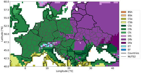
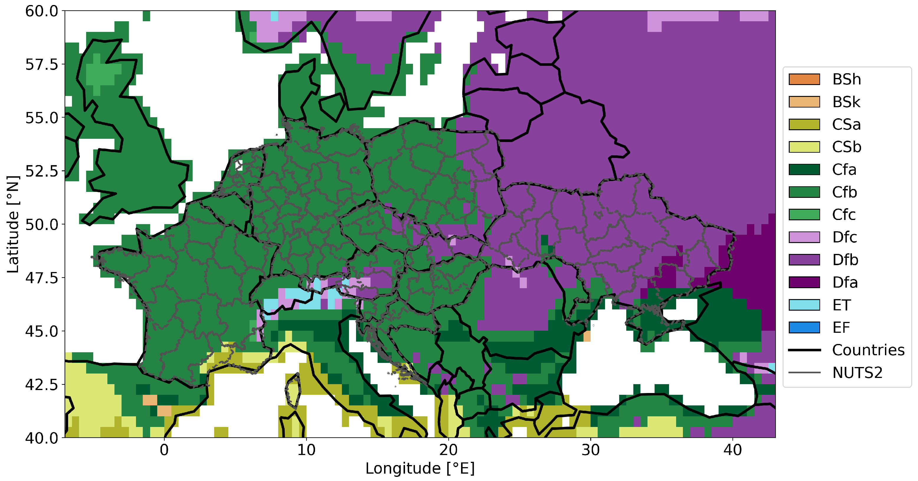
The focus of the study area is Ukraine, including its illegally occupied territories. However, for the training of the model, we use training data across Europe (Figure 1). The countries with available crop yield data in this study include France, the Netherlands, Germany, Austria, Czechia, Poland, Slovenia, Slovakia, Hungary, Croatia, and Ukraine. Throughout the manuscript, we refer to datasets from all countries except Ukraine as EU countries for simplicity. These EU countries predominantly fall within the Cfb climate classification of the Köppen–Geiger system, corresponding to a warm temperate, fully humid climate with hot summers, whereas Ukraine and eastern parts of Poland and Slovakia were predominantly classified as Dfb, characterised by snow, full humidity, and hot summers [32].
Figure 1.
Study area showing the regions with available crop yield data—on which we focus in this study—and the Köppen–Geiger climate classification. Predominant classes are Cfb and Dfb, which stand for warm temperate, fully humid climate with hot summers and snow, full humidity, and hot summers, respectively.
Sowing and harvesting periods are similar across these regions: both in Ukraine and central Europe, sowing of winter wheat, spring barley, and maize starts in September, March, and April, respectively. In Ukraine, harvesting of winter wheat and spring barley begins in July, and for maize in September. In central Europe, winter wheat and spring barley harvesting starts in early July (Austria, Croatia, Hungary, and Slovakia) or mid-July (Czechia, Germany, France, Poland, and Slovenia), while maize harvesting occurs from early October across all EU countries [33,34].
For detailed analysis, we focus specifically on areas in Ukraine impacted by the conflict in 2022. These are categorised into two groups: partially occupied regions, which have partially been under Russian control since the war’s onset, and regained regions, which were relatively quickly liberated by Ukraine during 2022. The term “areas under attack” collectively refers to both partially occupied and regained regions. The partially occupied regions are Donetsk (NUTS2-code UA14), Zaporizhzhya (UA23), Luhansk (UA44), and Kherson (UA65). Please note that we do not have data for Crimea, hence it is not listed here. The regained regions include Kyivska (UA32), Mykolayiv (UA48), Sumy (UA59), Kharkiv (UA63), and Chernihiv (UA74). These regional definitions align with those presented in NZZ [35].
2.2. Data
2.2.1. Crop Yield Data
We utilise crop yield data collected at the NUTS2 level from national statistical offices; for France, we use the publicly available dataset compiled by Schauberger et al. [36], while data from the other countries was obtained from national statistical offices. The data span from 2000 to 2022, with some years missing for certain countries, and Ukrainian data available only from 2007 to 2022. Spatial detail varies by country, ranging from NUTS2 to NUTS4 regional levels. Since Ukrainian data are available at the NUTS2 level, all other country data are resampled to NUTS2 to ensure spatial comparability by taking the arithmetic mean of all NUTS3 level regions laying within (Figure 1). We preserve the original crop yield data and did not calculate anomalies from it nor detrend it as these adjustments would oversimplify the problem and remove meaningful spatial variations. Instead, the machine learning model is also trained with the year as predictor so that it implicitly considers trends itself.
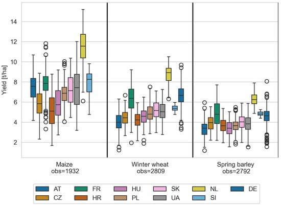
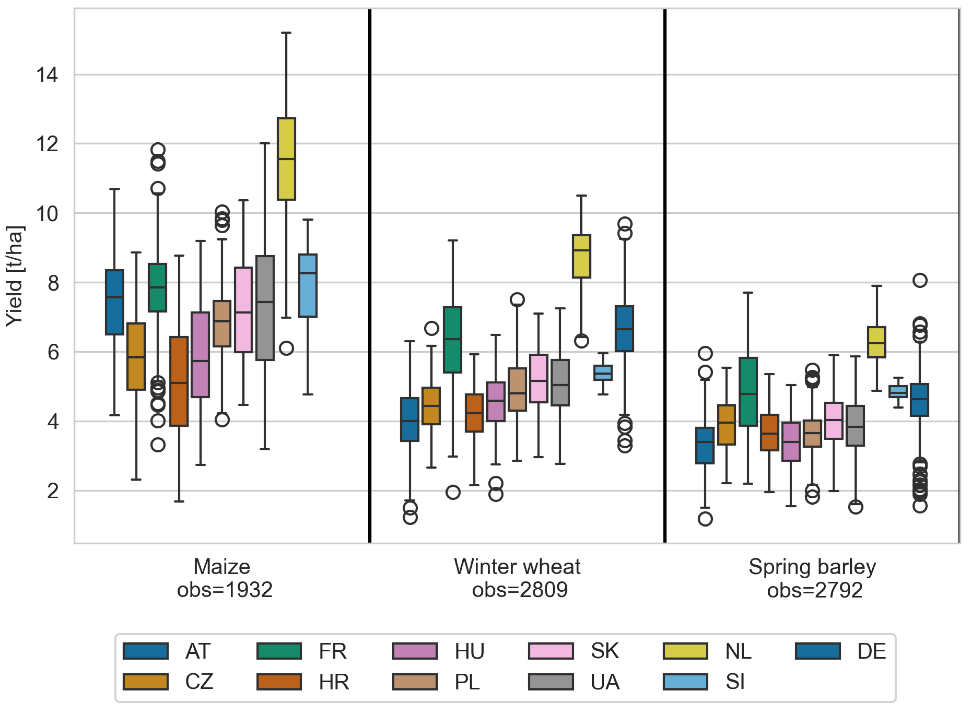
The crop yield data cover the predominant crops: maize, winter wheat, and spring barley, expressed in tonnes per hectare (t/ha). The distributions of crop yields are shown in (Figure 2), revealing similar patterns across most countries and crops. The Netherlands are a notable outlier, exhibiting significantly higher yields across all crops. For the other countries, average yield ranges span approximately 4 to 9 t/ha for maize, 3 to 7 t/ha for winter wheat, and 3 to 5 t/ha for spring barley, with Ukrainian yields comparable to most other countries. To ensure training on diverse conditions, we included all countries in this study.
Figure 2.
Crop yields per country and crop type. Country codes refer to: AT for Austria, CZ for Czechia, FR for France, HR for Croatia, HU for Hungary, PL for Poland, SK for Slovakia, UA for Ukraine, NL for Netherlands, SI for Slovenia, and DE for Germany. Outliers of the boxplot are indicated as circles.
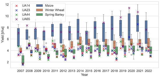
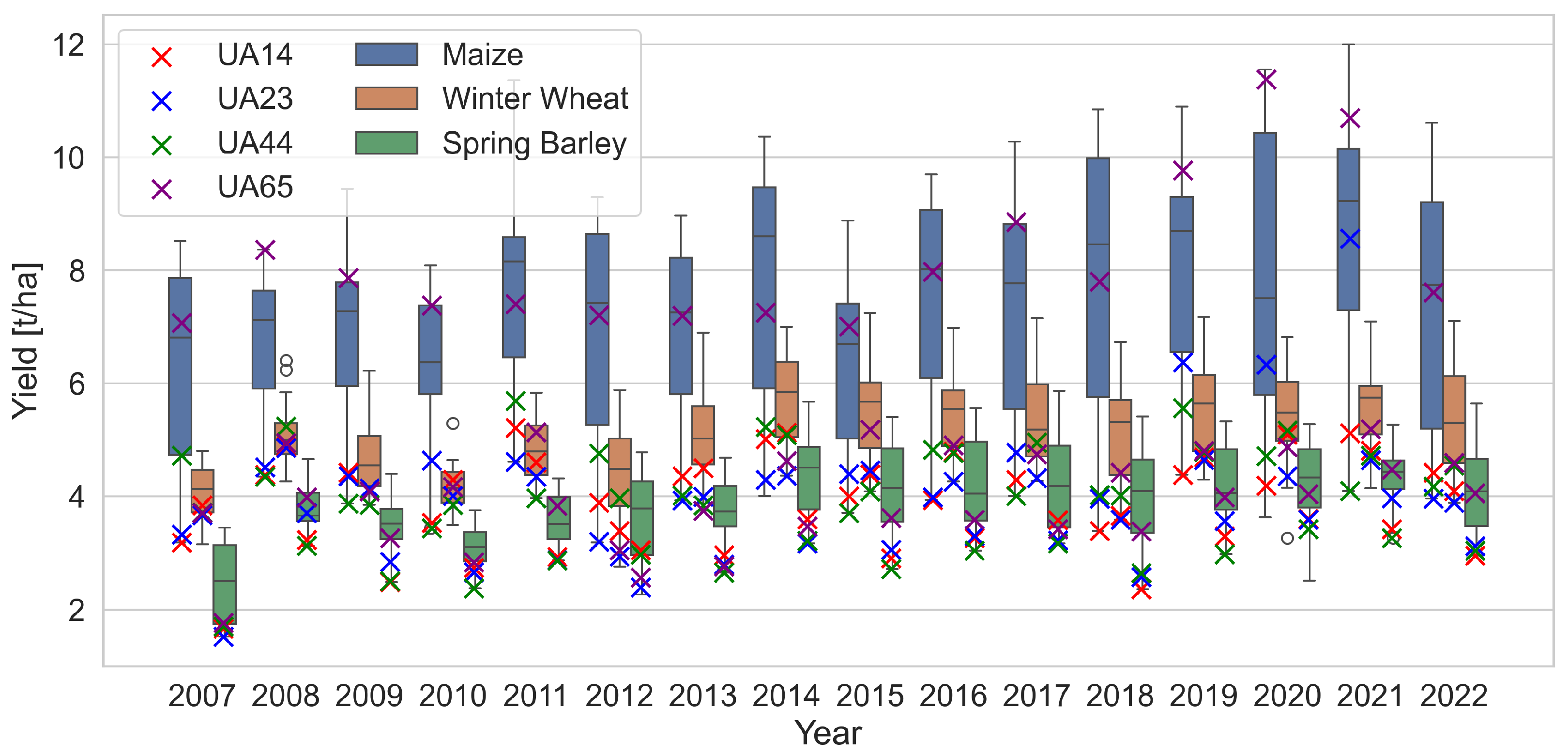
Figure 3 presents the interannual yield variations for Ukraine and its four partially occupied regions. A general increasing trend is evident over the past 15 years, and noticeably lower yields in 2022 relative to previous years throughout the country. Yields in partially occupied regions consistently fall below the national average even before the start of the war, except for maize in the region UA65.
Figure 3.
Ukraine crop yields per year and crop type. Crop yields for areas that have been partially occupied since 2022 are indicated by an ×. The NUTS2 codes stand for: UA14—Donetsk, UA23—Zaporizhzhya, UA44—Luhansk, and UA65—Kherson.
2.2.2. Predictor Data
The predictor datasets used in this study are categorised into meteorological and EO groups. Using these two types of predictors is motivated by their demonstrated reliability as predictors for crop yield modelling [8,37,38,39]. While meteorological predictors accurately represent the weather conditions affecting crop development, EO data capture the actual observed state of crops and soils.
Meteorological predictors are derived from ERA5-Land [40] and include total precipitation (m), 2 m temperature (K), potential evaporation (m), surface net solar radiation (Jm−2), evaporation from vegetation transpiration (m), and volumetric soil water layer 1 (m3m−3). Although the last two predictors are not meteorological, we include them here since these are key drivers of crop growth and are driven by meteorological conditions. Since these predictors are still modelled datasets, independence from EO-based datasets is given. The EO-based predictors comprise EVI (unitless) from MODIS [41], soil moisture (SM) (m3m−3) from the ESA CCI soil moisture combined version 9.1 [42] (employing the gap-filled version [43] available at https://doi.org/10.48436/hcm6n-t4m35), and Vegetation Optical Depth (VOD) (unitless) available at https://doi.org/10.48436/t74ty-tcx62 from the VOD climate archive version 2 which is a microwave-based indicator of vegetation water-content, thus, related to above ground biomass [44]. Please note that we used two soil moisture datasets, one from modelled data and one from EO data, to have information about how much soil moisture is expected as a result of meteorological forcing and how much is actually observed (including irrigation and other non-meteorological impacts). In addition to these predictors, we also used the year in which yields are observed as predictor, since crop yields exhibit increasing trends over time. The variable year is used in all model setups.
Regarding spatial and temporal resolution, ERA5-Land provides hourly data at 0.1° resolution; SM and VOD datasets have daily frequency and 0.25° spatial resolution; and MODIS (MOD13C1) EVI offers 16-day composites at 0.05° resolution. We did not use a finer spatial resolution of MODIS data since we are interested in large-scale patterns (i.e., NUTS2 level) and want to have a similar spatial resolution of all predictors for consistency. Generally, predictors with a high spatial resolution like Sentinel-2 or Landsat 5, 7, and 8 could of course provide more information about field-scale variabilities, however, we decided to not use them for these reasons: (1) The used datasets provide longterm, consistent, and well-validated information for crop monitoring with lower noise than equivalent high spatial resolution data. (2) High temporal resolution of the used datasets mitigates issues of cloud cover. (3) Large-scale agriculture in Ukraine is well suited for this spatial resolution. (4) Using high resolution data at European level for model training requires huge computational capacities.
2.2.3. Data Preparation
Predictor datasets are aggregated per NUTS2 area by computing the median of all observations within each region. For EVI, which has a finer spatial resolution, pixels with a land cover other than cropland are mask-based to isolate signals from cropland areas (i.e., only pixels with a majority of agricultural areas are used) [45]. This masking step is not applied to other datasets due to their coarser spatial resolutions, which primarily capture large-scale variability. Also, at these resolutions, masking would be difficult as the pixels contain a large variety of land covers. In Ukraine—mainly consisting of agricultural areas—masking is anyway less relevant than in central Europe where land cover is more diverse and agricultural areas smaller. Following spatial aggregation, all datasets are temporally resampled to monthly resolution with lead times (LTs) ranging from 1 to 4 months prior to the harvesting season, where LT1 refers to the last month before harvesting. The harvesting season start dates are taken as defined in Section 2.1. We use fixed dates per country for all years. By doing so, we do not account for yearly variations of the start of the harvesting season, but these fixed dates are the most precise information we have. We use data from different LTs to have information of the predictors throughout the growing season.
2.3. Modelling
2.3.1. Crop Yield Estimation Model
Crop yield estimations are implemented at the start of the harvesting season using two model types: Extreme Gradient Boosting (XGB) as the baseline and ANN under various configurations. All models employ a leave-one-year-out cross-validation approach, where testing solely utilises Ukrainian data from the excluded year. The training and fine-tuning processes exclude the data from the left-out year. The model configurations applied in this study are in Table 1. TL is a tool with which deep learning models are trained and finetuned in different domains (Section 1). Here, we used this approach to train an ANN model using EU countries crop yield data and finetune it using Ukrainian crop yield data—both at subnational level (NUTS2). The model we used for TL is an ANN. The ANN architecture comprises an input layer, two hidden layers with 64 and 32 nodes, respectively (both incorporate batch normalisation and a 30% dropout), and an output layer. Further details about the model can be found on github as indicated at the end of the paper. Models are trained fully on the training dataset, while in the TL setups, all layer weights are adjusted during an additional fine-tuning phase using the fine-tuning dataset Table 1. This last step is the difference between classical deep learning techniques and transfer learning: the model is retrained (adjusting the model weights from the initial training) to adjust to the new region.
Table 1.
Model setups used in this study. UA stands for Ukraine, CE for Central Europe, met for meteorological predictors, and eo for Earth observation.
The two models ANN_tl_eo and ANN_tl_met are the relevant ones for the assessment of war-related crop yield losses (see Section 2.3.2). The other models are used as baseline to see if these models perform sufficiently well. The XGB model undergoes hyperparameter tuning for each run via Sklearn’s GridSearchCV, using parameters summarised in Table 2.
Table 2.
Parameter values for the hyperparameter-tuning of the XGB model.
For each train/validation split of the leave-one-year-out cross-validation, performance is evaluated by calculating the mean absolute percentage error (MAPE) and R2 between observed and estimated yields. The two metrics are chosen because R2 provides a widely used and easily comparable measure to other studies, while MAPE expresses the error as a percentage deviation from observations, offering intuitive information valuable to farmers and decision-makers which is also well comparable between different crops. The metrics are calculated as follows:
Additionally, we assess feature importance within our models to evaluate the influence of different predictors to better understand the models and potentially gain trust in them. Specifically, we compute the permutation importance of the ANN_tl_eomet model before and after fine-tuning. This analysis is performed within the leave-one-year-out cross-validation framework, with permutation importance calculated ten times for each validation year to ensure robustness.
2.3.2. Estimation of War-Related Yield Losses
This study aims to quantify war-related yield losses in 2022. As mentioned before, war-related crop yield losses are a combination of field abandonment and crop yield losses on fields which were still used. Here, we focus on the latter since the first has already been quantified in other studies, e.g., He et al. [19], Dai et al. [20]. War-related crop yield losses are differences between potential crop yields given the meteorological conditions, and observed yields. To assess this, we need two types of information: (1) potential yields and (2) achieved crop yields. Potential crop yields are defined as maximum reachable yield in given meteorological conditions and environments by certain crops, as determinable, for example, by simulation models [46]. Here, we assess potential yields by implementing a crop yield estimation model based on meteorological data. This approach does not show potential yields as the absolute maximum possible (including optimised management) as simulation models do. Instead, it shows likely achievable crop yields by farmers under given meteorological conditions, since the model is trained with achieved crop yields from before the war. Therefore, we expect it to be a reliable reference of what would have been obtained without war impacts. This information is then compared with the actually obtained yields. Achieved yields are most reliably available as national yield statistics. In this study, we have 2022 crop yield data available; thus, we use this as reference of achieved yields. However, in conflict areas, measured crop yield data are often not available or subject to high uncertainties. Hence, we also need a model-based alternative for better generalisability of our results. Thus, we also set up an EO-based crop yield estimation model. Using only EO data provides the model with information about the actual state of crops, representing both meteorological and war-related causes. Our definition of war-related crop yield losses is the difference between meteorological yield estimations and observed yields (or EO-based yield estimations), since we expect the meteorological-based yield estimations to be higher than the observed (or EO-based) ones.
3. Results
3.1. Validating the Models
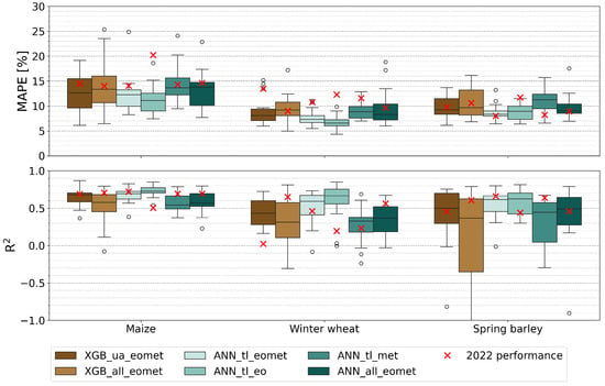
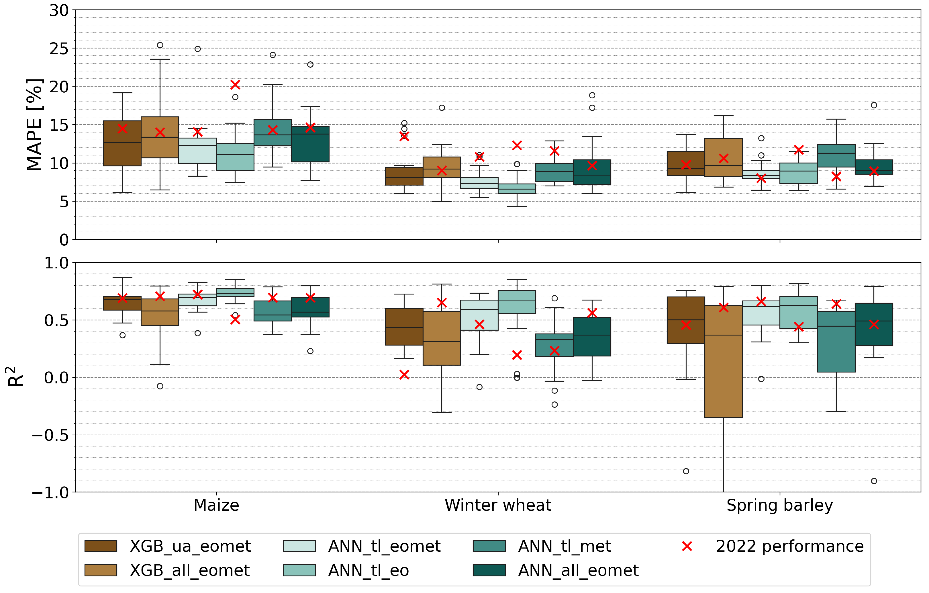
The validation results of the models are summarised in Figure 4, revealing distinct performance differences across crops and model configurations. For maize, all models demonstrate relatively strong performance, with mean R2 values ranging from 0.55 to 0.73 and mean errors between 11 and 14%. The best results are achieved by ANN_tl_eo, which attains the highest mean R2 and lowest error, whereas the lowest performance is observed in models trained directly on all countries (including UA) data (ANN_all_eomet and XGB_all_eomet) and ANN_tl_met.
Figure 4.
Validation of the crop yield estimations. Model setups are described in Table 1. Outliers of the boxplot are shown as circles.
For winter wheat, performance diverges more, with mean R2 values spanning 0.29 to 0.65 and lower MAPE from 6.5 to 9.8%. ANN_tl_eo again yields the best results, while XGB-based models, ANN_tl_met, and ANN_all show significantly lower performance (mean R2 < 0.45 and errors near 8–9%).
Spring barley exhibits less variation among models compared to the other crop types, with ANN_tl_eo and ANN_tl_eomet outperforming others by a margin of over 0.10 in mean R2 (above 0.60 compared to 0.50 or below for the rest).
Overall, TL models utilising EO data (ANN_tl_eomet and ANN_tl_eo) perform strongly for maize (mean R2 > 0.60), while ANN_tl_met yields moderate results (R2 between 0.35 and 0.55). The TL-based approaches ANN_tl_eomet clearly represent the most effective utilisation of Ukrainian data: they significantly outperform models trained directly on all countries (XGB_all_eomet, ANN_all_eomet), as well as the solely Ukraine-trained model XGB_ua_eomet. Although the performance gain of TL over XGB_ua_eomet is small for maize (R2 improvement of about 0.01), for winter wheat and spring barley, the advantage is more pronounced, with R2 increases exceeding 0.11. Notably, ANN_tl_eo consistently outperforms ANN_tl_eomet, indicating that including additional predictors can also reduce model performance.
The two validation metrics generally agree well within each crop type, as model configurations with higher mean R2 typically correspond to lower mean errors. However, this agreement does not extend across crops; maize models exhibit the highest mean R2 but also the largest mean errors.
3.2. Feature Importance of the Model
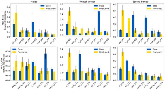
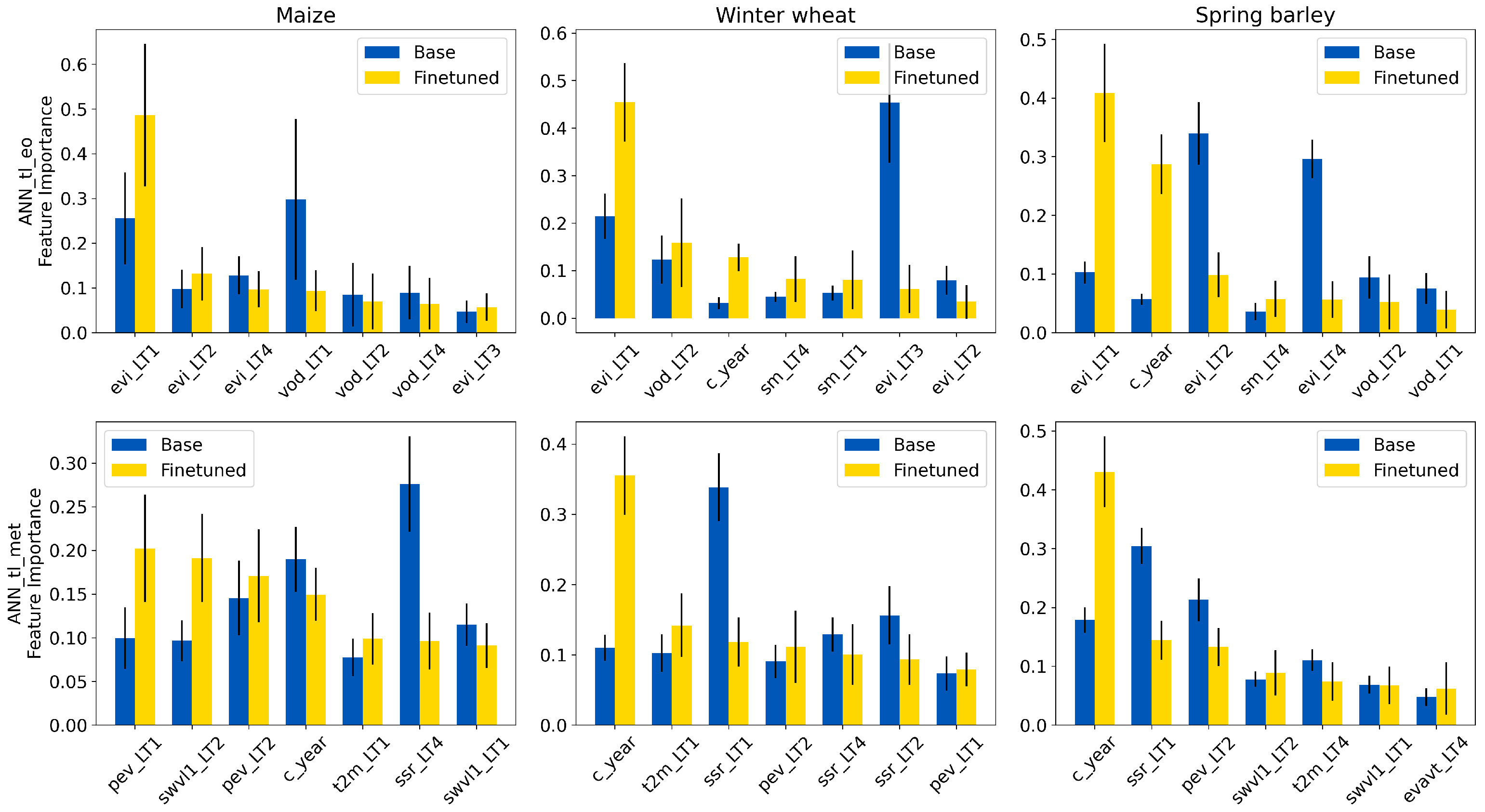
Feature importance analysis of ANN_tl_eo and ANN_tl_met models (Figure 5) demonstrates several notable findings: (1) EVI with LT1 is for all crops the most important EO predictor after finetuning, while the meteorological model does not have a single most important parameter. (2) Predictors with shorter lead times generally play a more important role, although there are exceptions: EVI LT4 is the third most important predictor for maize and SM LT4 is the third most important predictor of winter wheat and spring barley. (3) Fine-tuning substantially impacts the ranking and magnitude of feature importance, often leading to a more pronounced weighting of the top predictor or changing it. (4) The model trained solely on EU countries data often places greater emphasis on longer LTs: for ANN_tl_eo winter wheat and spring barley, the most important predictor before finetuning is from LT 3 and 2 (EVI), respectively, and ANN_tl_met for maize even LT 4 (surface net solar radiation) is the top predictor before finetuning. (5) The year variable is for both models among the top predictors for winter wheat and spring barley (for ANN_tl_met even twice the most important one). This shows that temporal trends have a major impact on Ukraine’s crop yields, which can also be seen in Figure 3.
Figure 5.
Feature importance of the predictors in the ANN_tl_eomet model before and after fine-tuning. The error bars are based on the leave-one-year-out setup and ten permutation importance runs. The abbreviations are based on the predictor and their LT. Predictor abbreviations are as follows: t2m is 2 m temperature, pev is potential evaporation, ssr is surface net solar radiation, swvl1 is volumetric soil water layer 1, ERA5-Land, evi is enhanced vegetation index, VODCA_CXKu is vegetation optical depth, and sm is soil moisture.
3.3. 2022 Model Performance and War-Related Yield Losses
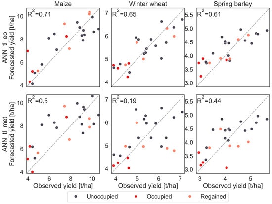
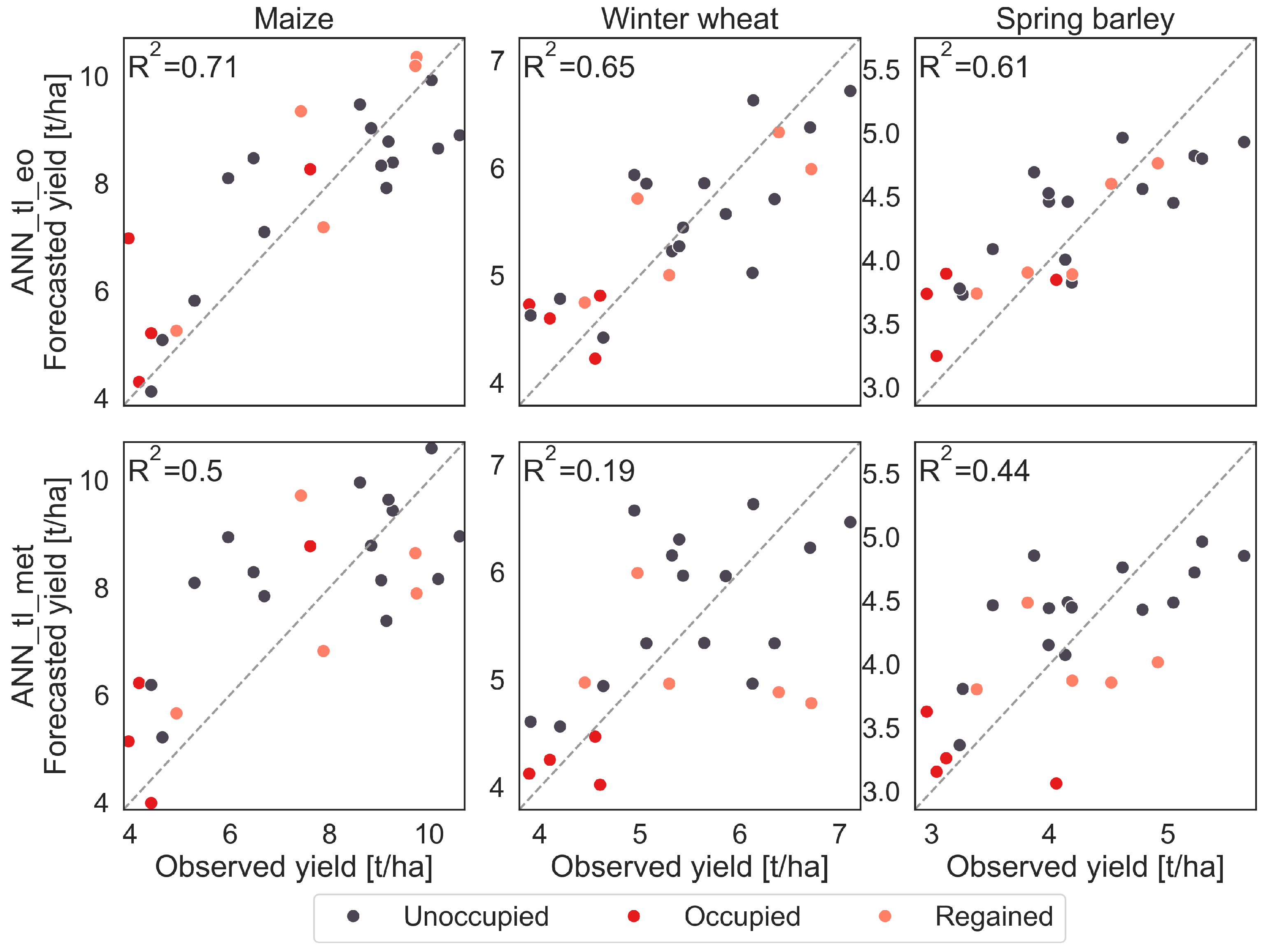
The performance of the models in 2022 presents a complex picture (red cross in Figure 4). Most models and crops exhibit above-average MAPE, though the R2 values vary: for maize and spring barley, all models except the EO-based ANN_tl_eo remain at or above average, whereas for winter wheat, only models trained on all countries data (XGB_all_eomet and ANN_all_eomet) exceed this threshold. Since we want to use ANN_tl_eo and ANN_tl_met for quantifying war-related yield losses, we analyse it in more detail by looking at the distribution of the observed and estimated yields (Figure 6). Partially occupied regions consistently display among the lowest yields, as in all years, with estimations of both models tending to slightly overestimate actual yields. In regained areas, the pattern is less clear, with several regions exhibiting relatively high yields, which the models sometimes over- and sometimes underestimate. Generally, the performance of ANN_tl_eo is much better than that of ANN_tl_met in 2022 as already seen in Figure 4.
Figure 6.
Estimated maize, winter wheat, and spring barley yields of Ukrainian regions after the start of the war in 2022 using the ANN_tl_eomet model. Dashed line indicates x = y.
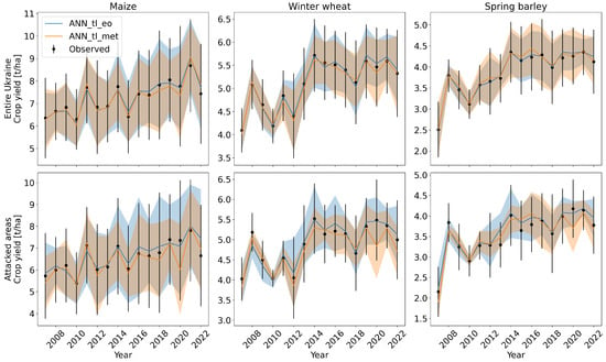
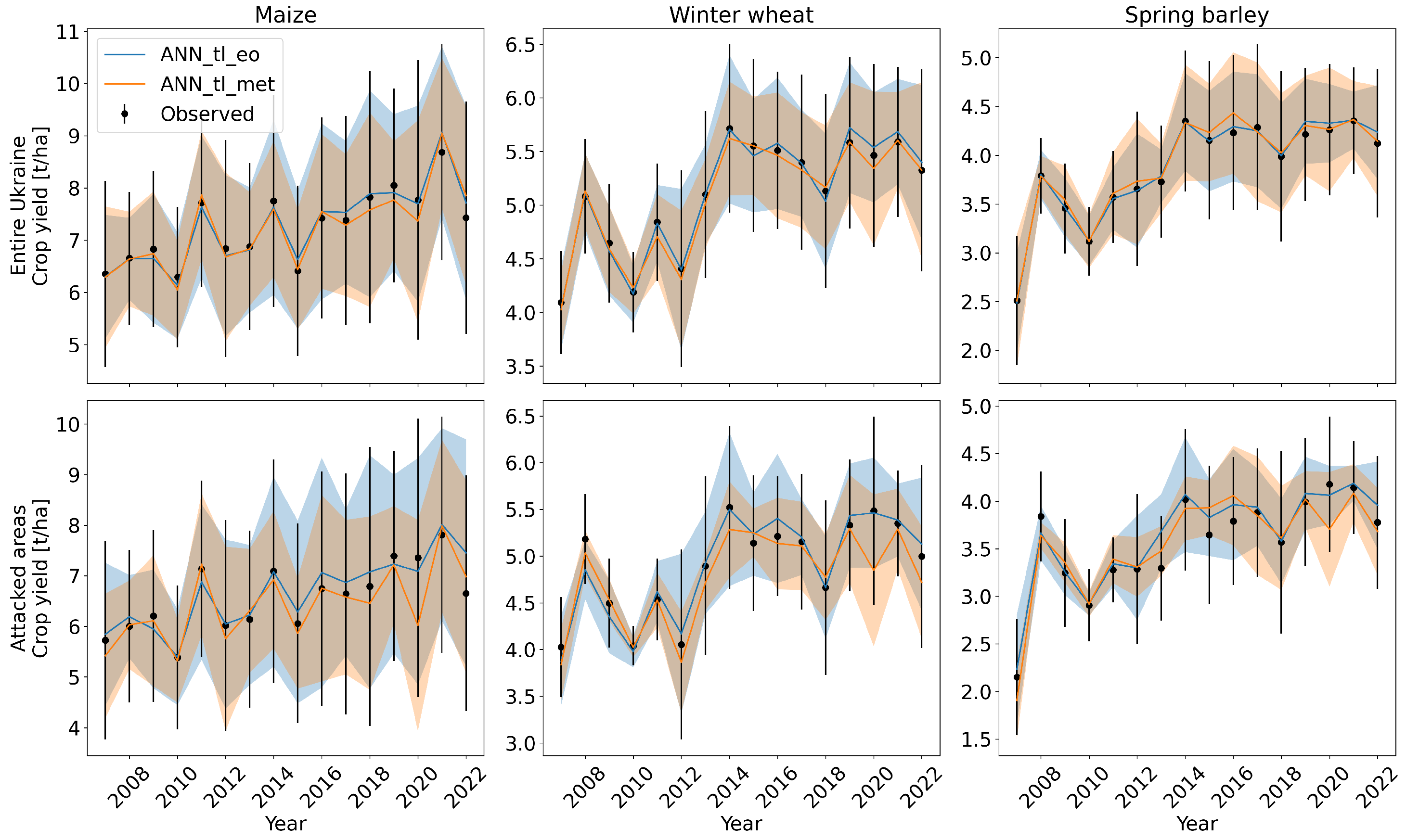
Visual inspection of time series (Figure 7) confirms that 2022 yields are lower than in preceding years. The three years preceding the war are among the most productive for the conflict-affected zones, while 2022 yields fall below this baseline. This discrepancy is not mirrored in meteorological yield estimates, which, although lower in 2022 than 2021, are similar to 2020 levels—a year with much higher observed yields. Meteorological estimates have a lower accuracy in both 2020 and 2022, whereas EO-based estimates generally provide superior annual mean yield estimations. In 2022, however, the EO-based model substantially overestimates yields nationwide (Figure 7, top row), with a more pronounced overestimation within conflict-affected areas (Figure 7, bottom row).
Figure 7.
Time series of the mean crop yields and their estimations for all regions in the Ukraine on top and for the most impacted regions (the partially occupied regions UA14: Donetsk, UA23: Zaporizhzhya, UA44: Luhansk, and UA65: Kherson as well as the regions under attack: UA32: Kyivska, UA48: Mykolayiv, UA59: Sumy, UA63: Kharkiv, and UA74: Chernihiv) below. The error bar and area around the observed yields and estimations show the standard deviation between the different areas of the considered year.
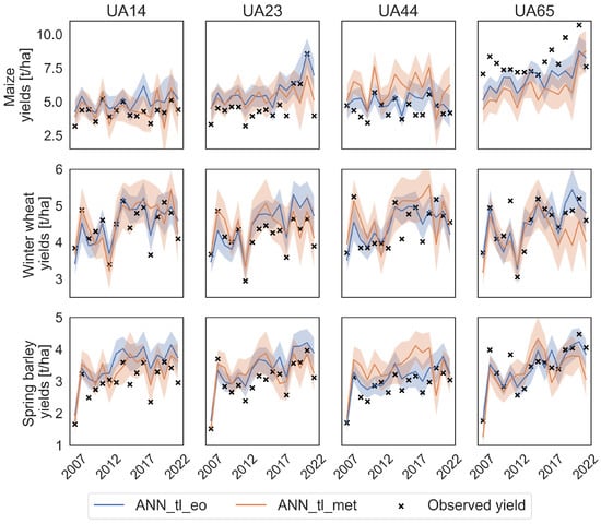
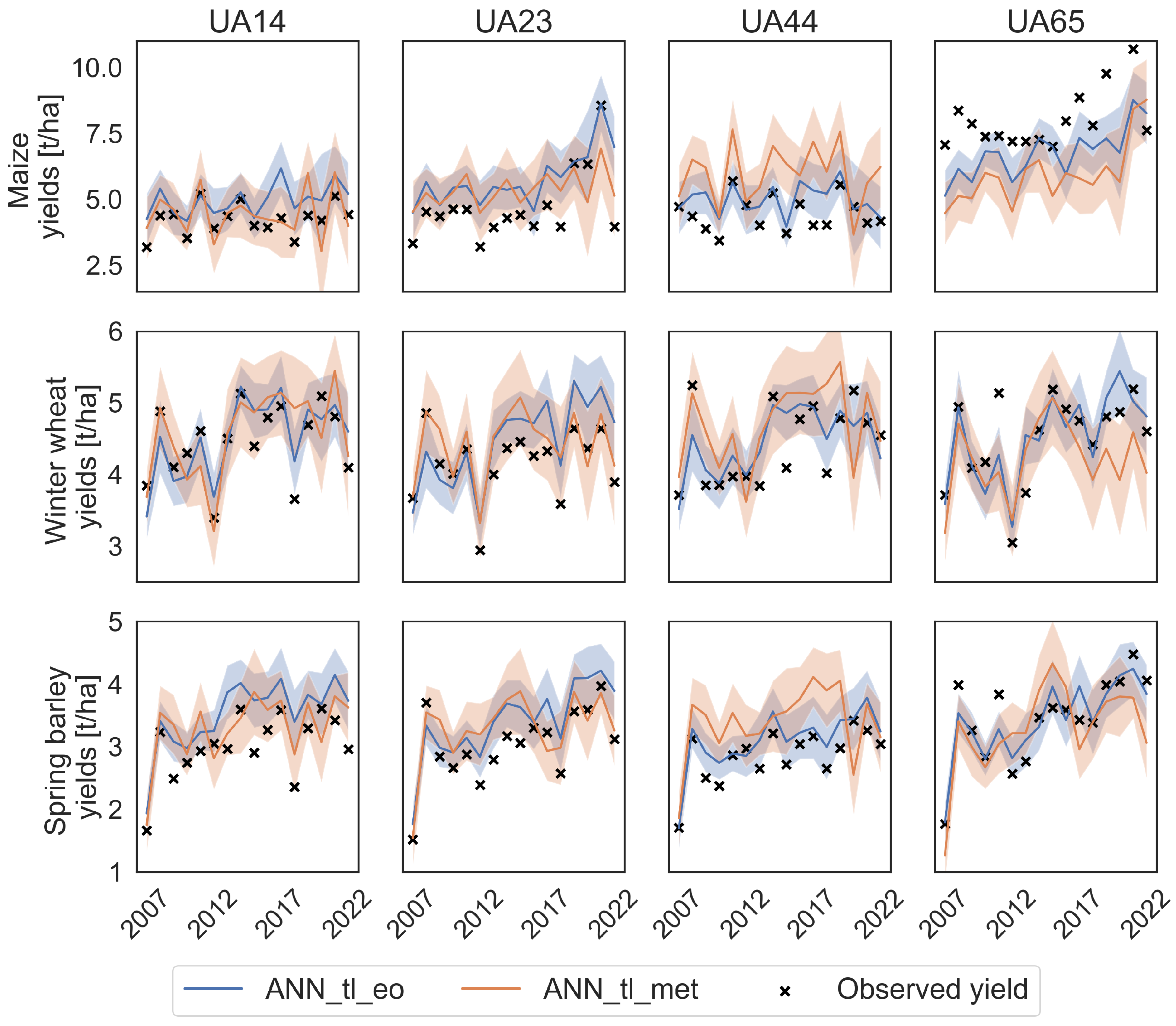
Additionally, model performance in capturing interannual yield variability at the individual NUTS2 region level is highly diverse, as shown in Figure 8 and Table 3. ANN_tl_met does not work well for any region and crop (all ≤ 0.40), while ANN_tl_eo achieves for winter wheat and spring barley, at least, some useful results (e.g., winter wheat UA14 and spring barley UA65). After merging all NUTS2 areas under attack together (Figure 7), models demonstrate high performance, with strong agreement between predicted and actual mean yields of the areas and their standard deviations (Table 3).
Figure 8.
Timeseries of the crop yields and their estimations of the four most impacted regions (UA14: Donetsk, UA23: Zaporizhzhya, UA44: Luhansk, and UA65: Kherson). The error area around the estimation is the estimated yield +/− the root mean square error of the model.
At this level of aggregated regions, we also tried to quantify war-related yield losses. Our assumption was that meteorological crop yield estimations are higher than the observed and EO-based ones, with the difference indicating war-related crop yield losses. The bottom row of Figure 7 shows that this is not the case. In 2022, meteorological estimations of winter wheat and spring barley are lower than observed yields. For maize, we observe a slight overestimation of crop yields, but the EO-based estimations are always highest, with observed yields being 14% lower than EO-based estimations (7 t/ha and 6 t/ha), while no significant losses are found for spring barley and winter wheat.
4. Discussion
4.1. Crop Yield Data
Crop yield data play a key role in all analyses in this paper, and uncertainties herein are acknowledged. Official crop yield statistics are typically based on expert estimates of average regional yields and are inherently subject to bias and uncertainty. These challenges are exacerbated in conflict settings, where data collection becomes more difficult and more prone to error. Although quantifying these uncertainties is challenging, recognising them is crucial as a limitation of this study’s approach. Despite this limitation, the data have been carefully checked and still provide a useful baseline for the upcoming analysis.
4.2. Analysis of Model Performance
The crop yield estimation model serves as the foundation for further analyses. Two of our models, ANN_tl_eomet and ANN_tl_eo, demonstrated consistently strong results across all three crops, with low errors (<10% for barley and wheat and around 13% for maize) and high R2 values around 0.6 (see Figure 4). With the onset of the war, a decline in model performance might have been anticipated, given that meteorological conditions could be overshadowed by war-related impacts, and EO predictors might detect new patterns associated with substantial field abandonment or war-related crop yield changes. This effect is apparent for the EO model, where 2022 ranks among the worst-performing years due to elevated errors and reduced R2 values. Although the other two TL models also exhibit comparatively high errors in 2022, their R2 scores indicate above-average performance.
Examination of observed versus estimated yield distributions (Figure 6) reveals significant overestimations by both models (ANN_tl_eo and ANN_tl_met) of yields in the partially occupied regions, reflecting the expected loss of production potential due to war-related factors. However, this overestimation is not consistently greater in the partially occupied areas than in many non-occupied regions, and regained regions are often underestimated. This leads to the conclusion that the models are not able to correctly detect war-impacts at NUTS2 level. This is also indicated by the low performance of the two models per region (Table 3). For maize, both models have a very low model performance in all occupied regions, except for the meteorological model in UA14 (R2 = 0.4). Also, the other crops show in most occupied regions much worse performance at the individual region-level than when aggregated.
4.3. War-Related Yield Losses
The primary objective of this study, however, was not to compare losses at the regional level but to quantify aggregated countrywide yield losses. Therefore, the low model performance for the individual regions does not hinder the estimation of war-related crop yield losses. This is especially the case since the performance of the model, when being aggregated to multiple regions (Region All and Attacked in Table 3), is high for both models and all three crops. Visual inspection of time series data (Figure 7 and Figure 8) confirms robust model performance at the aggregated level (combining all regions under attack) (Table 3). The inherent noise and potential other factors at finer regional scales appear to diminish model accuracy (Figure 8 and Table 3). Aggregation to coarser spatial scales reduces uncertainties in both predictors and yields, resulting in improved model performance.
The EO-based model (ANN_tl_eo) consistently overestimates 2022 crop yields for the national average and specifically within conflict-affected regions (Figure 7). The overestimation is particularly pronounced for maize, exceeding levels observed in previous years, and suggests war-related yield losses. Nonetheless, two factors temper this interpretation: firstly, the overestimation pattern is not evident for winter wheat and spring barley. For these crops, overestimation in 2022 is similar to or even lower than those in other years, such as 2016 for winter wheat and 2013 for spring barley within attacked areas. Secondly, meteorological models do not replicate the clear 2022 overestimation; they even underestimate winter wheat and spring barley yields in conflict zones, indicating that actual yields were rather high relative to meteorological expectations.
Maize yields are clearly overestimated in 2022 by the EO-based model. This anomaly is clearly more pronounced than in other years; thus, random variation of the model or other factors like impacts of predictor and crop yield uncertainties, crop calendar mismatch, or model extrapolation cannot be the only reason, since these are similar in the years before the war. Thus, here we can see impacts of the war. Since maize is harvested later (starting in September) compared to spring barley and winter wheat (harvest starting in July), maize fields were more susceptible to abandonment before harvest or were not even sown anymore. Also, winter wheat was already sown before the start of the war and may still have grown but not been harvested due to land abandonment. The factor of land abandonment also explains why the EO model more effectively captures war-related impacts than the meteorological model. In summary, our approach detects approximately 14% maize yield losses (with estimations around 7 t/ha versus observed yields near 6 t/ha), while no significant losses are found for spring barley and winter wheat. However, given the overestimation of the EO model in years before the war, we cannot claim that all of it is related to war impacts. Also, we checked for significance of the differences which showed that there are no statistically significant differences between the two models (ANN_tl_eo and ANN_tl_met) and the observed yields (Table A1 in Appendix A). Generally, our initial premise of simply contrasting meteorological and EO-based estimations did not hold due to the strong influence of meteorological conditions on EO data and the complexities discussed above. This makes the EO model the most reliable model, since it implicitly corrects for meteorological conditions and also shows war-related impacts.
4.4. Comparison to Existing Studies
Other studies have reported more severe crop yield losses than those observed in our analysis. For instance, He et al. [19] estimated grain yield losses in conflict-affected areas at 7.58% due to land abandonment combined with a 33.02% decrease in crop yields on cultivated fields in attacked areas. Similarly, Chen et al. [2] estimated an average crop yield loss of approximately 37% for wheat, sunflower, and rapeseed. Both studies linked war-related crop yield losses to NDVI variations in 2022 compared to the years before the war. Lin et al. [21] predicted more substantial impacts on wheat and winter crops than the low changes we detected for winter wheat. Regarding land abandonment, Dai et al. [20] confirm findings from He et al. [19] showing that land abandonment alone caused crop yield losses between 7.5 and 9.5% for wheat, maize, barley, and sunflower.
These discrepancies are partly attributable to methodological differences, as the aforementioned studies rely exclusively on EO data without accounting for meteorological conditions. In addition, they also mainly use NDVI as an estimator for crop yield but no real crop yield data. Both differences limit direct comparability between our study and theirs. However, these studies in combination with the limitations in our study—as mentioned above—indicate that we underestimate the indirect war-related yield losses in this study. One likely cause is the coarser spatial resolution of our predictors (ranging from 5 to 25 km), contrasting with the subfield-level resolution available through Landsat, Sentinel-2, and Planet data in several other studies. Consequently, our method assesses average conditions over broader areas and cannot explicitly detect changes in individual fields like land abandonment. However, our results using meteorological data also imply that previous studies may overstate actual losses. Ukrainian farmers appear to have performed remarkably well, producing harvests close to those expected under meteorological conditions despite the ongoing conflict.
4.5. Transfer Learning Performance
The results presented here illustrate an additional valuable application of TL, with TL models consistently outperforming baseline approaches such as XGB_all_eomet and ANN_all_eomet. Notably, XGB did not benefit from the inclusion of EU countries data, as indicated by the decline in performance of XGB_all_eomet compared to XGB_ua_eomet, whereas most TL models surpassed ANN_all_eomet. Insights from feature importance analysis help explain these observations. In central Europe, longer lead times generally hold greater predictive importance, with EVI at LT2 identified as the most significant feature. Colder climatic conditions in Ukraine likely shift crop development stages, rendering shorter lead times more relevant for estimations.
Overall, the consistent similarity of the most important features before and after fine-tuning indicates that pretraining on EU countries data provides substantial benefits. The model effectively adapts to the Ukrainian context by emphasising shorter lead times, which appear more meaningful there. This result aligns with previous findings by Bohra et al. [26] and Wang et al. [28], who demonstrated that transfer learning is a powerful technique for training and applying crop yield models across different countries and even continents.
Furthermore, it is important to discuss differences in performance gains using TL. The larger improvements of TL for spring barley and winter wheat compared to maize mainly arise from a worse model performance of the non-TL models for these two crops: ANN_tl_eomet performs similarly well for all three crops with median R2 between 0.6 and 0.7. However, the best non-TL approach (XGB_ua_eomet) varies from around 0.4 to 0.7. Thus, it appears that simple models have a higher performance for maize and struggle to correctly predict spring barley and winter wheat which is in line with previous studies Bueechi et al. [8], Kern et al. [39]. Only TL is able to predict spring barley and winter wheat with a similar accuracy as maize.
4.6. Potential Improvements
Some final points need to be mentioned. Firstly, the fact that EO-based estimations outperformed estimations based on all predictors shows that feature elimination is still critical for deep learning models as also shown in other studies [47,48].
We also want to state again that we used fixed harvesting season start dates per country. This introduces uncertainties to the model, since the actual start date of the harvesting season differs from year to year. Hence, further improvements of model performance could be achieved by using the actual yearly start dates of harvesting season—information that we could unfortunately not get for our entire study area. Thirdly, we tested if removing countries from the pretraining dataset (EU-countries) could help to improve model performance. This was not successful. The model seems to generalise sufficiently with having all the training data available.
Ultimately, a further limitation is that both the official yield statistics, reported at NUTS2 level, and the EO predictors, with spatial resolutions of 5 km and coarser, aggregate over areas that can include both abandoned and actively cultivated fields; we cannot fully separate these two categories at this scale. On average, around 7% of fields in Ukraine were abandoned in 2022, rising to up to 20% in the most severely impacted regions [2,20]. As abandoned fields remain a minority of the area even in the worst-affected regions, we do not expect them to dominate the aggregated signal. However, their near-zero yield could bias results towards overestimating war-related yield losses in the most heavily impacted regions, which should be considered when interpreting results for such areas. At the same time, the coarse spatial resolution offers the advantage of long-term data availability and high temporal resolution, both critical for our modelling.
5. Conclusions
This study has tested a novel approach to quantifying war-related crop yield losses on the example of 2022 yields in Ukraine. Our idea was that meteorology-based estimations show potential crop yields while EO-based estimations represent the actually observed yields, and their difference, indirect war-related crop yield losses. The results did not confirm this hypothesis, particularly given that meteorology-based yield estimates frequently exceeded those based on EO data. Hence, further improvements to this method are needed before being able to clearly assess these losses. Still, we observed a signal of war-related yield losses for maize. Furthermore, we illustrated an additional practical application of TL to develop a reliable estimation system for Ukraine using data from central Europe. This approach facilitates overcoming data scarcity by leveraging existing datasets from data-rich regions.
Despite these advances, further research is required to clearly disentangle the roles of land abandonment and indirect war losses, in conjunction with meteorological factors, to fully understand the impact of conflict on agricultural production. To achieve this, potentially higher spatial resolution of predictor data is required, to better distinguish abandoned fields from still used ones and also distinguishing different crops. Such efforts remain essential for accurately assessing the consequences of wars on food security and for supporting effective policy responses.
Author Contributions
Conceptualisation, E.B. and W.D.; methodology, E.B. and W.D.; software, E.B.; validation, E.B.; formal analysis, E.B.; investigation, E.B.; resources, all authors; data curation, all authors; writing—original draft preparation, E.B.; writing—review and editing, all authors; visualization, E.B.; supervision, W.D.; project administration, M.P., E.B. and W.D.; funding acquisition, M.P., E.B. and W.D. All authors have read and agreed to the published version of the manuscript.
Funding
This study has been funded by the European Space Agency (ESA) in the framework of the project “YIPEEO: Yield prediction and estimation using Earth Observation” (Contract No. 4000141154/23/I-EF) and by Interreg Central Europe through the project Clim4Cast (Contract No. CE0100059) where most of the yield data were collected. Lukáš Dolák acknowledges support from AdAgriF-Advanced methods of greenhouse gases emission reduction and sequestration in agriculture and forest landscape for climate change mitigation (CZ.02.01.01/00/22_008/0004635). The authors acknowledge TU Wien Bibliothek for financial support through its Open Access Funding Programme.
Data Availability Statement
Crop yield data used in this study were acquired or obtained from (inter-) national statistical offices and personal connections, which unfortunately we cannot share. However, most data can be obtained from: https://ec.europa.eu/eurostat/ (accessed on 16 June 2025), https://www.statistik.at/en (accessed on 16 June 2025), and https://www.akcr.cz/ (accessed on 16 June 2025). The Python v 3.13 code used for the data preparation and crop yield forecasting is available at https://github.com/pbueechi/yipeeo (accessed on 16 June 2025).
Conflicts of Interest
The authors declare no conflicts of interest. The funders had no role in the design of the study; in the collection, analyses, or interpretation of data; in the writing of the manuscript; or in the decision to publish the results.
Abbreviations
The following abbreviations are used in this manuscript:
| ANN | Artificial Neural Network |
| CNN | Convolutional Neural Network |
| LSTM | Long Short-Term Memory |
| EO | Earth Observation |
| EVI | Enhanced Vegetation Index |
| FAPAR | Fraction of Absorbed Photosynthetic Active Radiation |
| LAI | Leaf Area Index |
| MAPE | Mean Absolute Percentage Error |
| ML | Machine Learning |
| MODIS | Moderate Resolution Imaging Spectroradiometer |
| NDVI | Normalized Difference Vegetation Index |
| NUTS | Nomenclature des Unités Territoriales Statistiques |
| SM | Soil Moisture |
| TL | Transfer Learning |
| LT | Lead Time |
| VOD | Vegetation Optical Depth |
| WOFOST | World Food Studies |
| XGB | Extreme Gradient Boosting |
Appendix A. Additional Table
Table A1.
T-Test results of crop yield estimates and observations. Eo met shows comparison between estimates from ANN_tl_eo and ANN_tl_met, obs met and obs eo show the comparison of ANN_tl_met and observed yields, and ANN_tl_eo and observed yields, respectively.
References
- Becker-Reshef, I. Measuring War’s Effect on a Global Breadbasket, 2022. NASA Earth Observatory. Available online: https://science.nasa.gov/earth/earth-observatory/measuring-wars-effect-on-a-global-breadbasket-150025/ (accessed on 26 May 2025).
- Chen, B.; Tu, Y.; An, J.; Wu, S.; Lin, C.; Gong, P. Quantification of losses in agriculture production in eastern Ukraine due to the Russia-Ukraine war. Commun. Earth Environ. 2024, 5, 336. [Google Scholar] [CrossRef] [Scilit]
- Panek-Chwastyk, E.; Da̧browska-Zielińska, K.; Kluczek, M.; Markowska, A.; Woźniak, E.; Bartold, M.; Ruciński, M.; Wojtkowski, C.; Aleksandrowicz, S.; Gromny, E.; et al. Estimates of Crop Yield Anomalies for 2022 in Ukraine Based on Copernicus Sentinel-1, Sentinel-3 Satellite Data, and ERA-5 Agrometeorological Indicators. Sensors 2024, 24, 2257. [Google Scholar] [CrossRef] [Scilit] [PubMed]
- USDA. Ukraine Agricultural Production and Trade; USDA: Washington, DC, USA, 2022. [Google Scholar]
- FAO. Impact of the War on Agricultural Enterprises; FAO: Rome, Italy, 2023. [Google Scholar]
- Lesk, C.; Anderson, W.; Rigden, A.; Coast, O.; Jägermeyr, J.; McDermid, S.; Davis, K.F.; Konar, M. Compound heat and moisture extreme impacts on global crop yields under climate change. Nat. Rev. Earth Environ. 2022, 3, 872–889. [Google Scholar] [CrossRef] [Scilit]
- Ben-Ari, T.; Adrian, J.; Klein, T.; Calanca, P.; Van der Velde, M.; Makowski, D. Identifying indicators for extreme wheat and maize yield losses. Agric. For. Meteorol. 2016, 220, 130–140. [Google Scholar] [CrossRef] [Scilit]
- Bueechi, E.; Fischer, M.; Crocetti, L.; Trnka, M.; Grlj, A.; Zappa, L.; Dorigo, W. Crop yield anomaly forecasting in the Pannonian basin using gradient boosting and its performance in years of severe drought. Agric. For. Meteorol. 2023, 340, 109596. [Google Scholar] [CrossRef] [Scilit]
- Shelestov, A.; Shumilo, L.; Yailymova, H.; Drozd, S. Crop Yield Forecasting for Major Crops in Ukraine. In 2021 IEEE International Conference on Information and Telecommunication Technologies and Radio Electronics (UkrMiCo); IEEE: New York, NY, USA, 2021; pp. 35–38. [Google Scholar] [CrossRef] [Scilit]
- Franch, B.; Vermote, E.; Skakun, S.; Santamaria-Artigas, A.; Kalecinski, N.; Roger, J.C.; Becker-Reshef, I.; Barker, B.; Justice, C.; Sobrino, J. The ARYA crop yield forecasting algorithm: Application to the main wheat exporting countries. Int. J. Appl. Earth Obs. Geoinf. 2021, 104, 102552. [Google Scholar] [CrossRef] [Scilit]
- Becker-Reshef, I.; Vermote, E.; Lindeman, M.; Justice, C. A generalized regression-based model for forecasting winter wheat yields in Kansas and Ukraine using MODIS data. Remote Sens. Environ. 2010, 114, 1312–1323. [Google Scholar] [CrossRef] [Scilit]
- Kussul, O.; Kussul, N.; Skakun, S.; Kravchenko, O.; Shelestov, A.; Kolotii, A. Assessment of relative efficiency of using MODIS data to winter wheat yield forecasting in Ukraine. In 2013 International Geoscience and Remote Sensing Symposium (IGARSS); IEEE: New York, NY, USA, 2013; pp. 3235–3238. [Google Scholar] [CrossRef] [Scilit]
- Franch, B.; Vermote, E.F.; Skakun, S.; Roger, J.C.; Becker-Reshef, I.; Murphy, E.; Justice, C. Remote sensing based yield monitoring: Application to winter wheat in United States and Ukraine. Int. J. Appl. Earth Obs. Geoinf. 2019, 76, 112–127. [Google Scholar] [CrossRef] [Scilit]
- Kolotii, A.; Kussul, N.; Shelestov, A.; Skakun, S.; Yailymov, B.; Basarab, R.; Lavreniuk, M.; Oliinyk, T.; Ostapenko, V. Comparison of biophysical and satellite predictors for wheat yield forecasting in Ukraine. Int. Arch. Photogramm. Remote Sens. Spat. Inf. Sci. 2015, XL-7-W3, 39–44. [Google Scholar] [CrossRef] [Scilit]
- Kogan, F.; Kussul, N.; Adamenko, T.; Skakun, S.; Kravchenko, O.; Kryvobok, O.; Shelestov, A.; Kolotii, A.; Kussul, O.; Lavrenyuk, A. Winter wheat yield forecasting in Ukraine based on Earth observation, meteorologicaldata and biophysical models. Int. J. Appl. Earth Obs. Geoinf. 2013, 23, 192–203. [Google Scholar] [CrossRef] [Scilit]
- Kokhan, S.; Popov, M.; Alpert, S.; Andreiev, A.; Drozdivskyi, O.; Temna, Y.; Sybirtseva, O.; Dorofey, Y. Fuzzy Cognitive Maps in Corn Yield Forecast. In Nexus of Sustainability; Studies in Systems, Decision and Control; Zagorodny, A., Bogdanov, V., Zaporozhets, A., Eds.; Springer: Cham, Switzerland, 2025; Volume 627. [Google Scholar] [CrossRef] [Scilit]
- Kryvoshein, O.; Kryvobok, O.; Zhylchenko, D. Yield prediction at field level. Ukr. J. Remote Sens. 2024, 11, 26–30. [Google Scholar] [CrossRef] [Scilit]
- Kokhan, S.; Dorozhynskyy, O.; Burshtynska, K.; Vostokov, A.; Drozdivskyi, O. Improved approach to the development of the crop monitoring system based on the use of multi-source spatial data. J. Ecol. Eng. 2020, 21, 108–114. [Google Scholar] [CrossRef] [Scilit] [PubMed]
- He, T.; Zhang, M.; Xiao, W.; Zhai, G.; Wang, Y.; Guo, A.; Wu, C. Quantitative analysis of abandonment and grain production loss under armed conflict in Ukraine. J. Clean. Prod. 2023, 412, 137367. [Google Scholar] [CrossRef] [Scilit]
- Dai, K.; Cheng, C.; Kan, S.; Li, Y.; Liu, K.; Wu, X. Impact of Arable Land Abandonment on Crop Production Losses in Ukraine During the Armed Conflict. Remote Sens. 2024, 16, 4207. [Google Scholar] [CrossRef] [Scilit]
- Lin, F.; Li, X.; Jia, N.; Feng, F.; Huang, H.; Huang, J.; Fan, S.; Ciais, P.; Song, X.P. The impact of Russia-Ukraine conflict on global food security. Glob. Food Secur. 2023, 36, 100661. [Google Scholar] [CrossRef] [Scilit]
- Wagner, J.; Skakun, S.; Nair, S.S.; Sadeh, Y.; Baber, S.; Oliinyk, O.; Poliakov, D.; Vaskivskyi, B.; Misiura, O.; Kussul, N.; et al. Estimating Winter Crop Planted Areas with Remote Sensing Imagery 2 in War-Affected Ukraine 3. Available online: https://ssrn.com/abstract=5196729 (accessed on 26 May 2025).
- Qadir, A.; Skakun, S.; Becker-Reshef, I.; Kussul, N.; Shelestov, A. Estimation of sunflower planted areas in Ukraine during full-scale Russian invasion: Insights from Sentinel-1 SAR data. Sci. Remote Sens. 2024, 10, 100139. [Google Scholar] [CrossRef] [Scilit]
- Sadeh, Y.; Wagner, J.; Nair, S.S.; Oliinyk, O.; Belles, E.; Bibih, A.; D’Harboullé, L.; Bendahmane, H.; Gupta, M.; Becker-Reshef, I. National-Scale In-Season Field Boundaries of Ukraine Using Remote Sensing. Sci. Data 2025, 12, 833. [Google Scholar] [CrossRef] [Scilit] [PubMed]
- Bueechi, E.; Reuß, F.; Pikl, M.; Homolova, L.; Lukas, V.; Trnka, M.; Dorigo, W. Making optimal use of limited field-scale data for crop yield forecasting using transfer learning and Sentinel-1 and 2 data. Smart Agric. Technol. 2025, 12, 101567. [Google Scholar] [CrossRef] [Scilit]
- Bohra, A.; Nottmeyer, S.; Ren, C.; Chen, S.; Ma, Y. Advancing Corn Yield Mapping in Kenya Through Transfer Learning. Remote Sens. 2025, 17, 1717. [Google Scholar] [CrossRef] [Scilit]
- Ma, Y.; Liang, S.Z.; Myers, D.B.; Swatantran, A.; Lobell, D.B. Subfield-level crop yield mapping without ground truth data: A scale transfer framework. Remote Sens. Environ. 2024, 315, 114427. [Google Scholar] [CrossRef] [Scilit]
- Wang, A.X.; Tran, C.; Desai, N.; Lobell, D.; Ermon, S. Deep transfer learning for crop yield prediction with remote sensing data. In 1st ACM SIGCAS Conference on Computing and Sustainable Societies; COMPASS 2018; Association for Computing Machinery, Inc.: New York, NY, USA, 2018; Volume 18. [Google Scholar] [CrossRef] [Scilit]
- Khaki, S.; Pham, H.; Wang, L. Simultaneous corn and soybean yield prediction from remote sensing data using deep transfer learning. Sci. Rep. 2021, 11, 11132. [Google Scholar] [CrossRef] [Scilit] [PubMed]
- Ma, Y.; Zhang, Z.; Yang, H.L.; Yang, Z. An adaptive adversarial domain adaptation approach for corn yield prediction. Comput. Electron. Agric. 2021, 187, 106314. [Google Scholar] [CrossRef] [Scilit]
- Joshi, A.; Pradhan, B.; Chakraborty, S.; Varatharajoo, R.; Gite, S.; Alamri, A. Deep-Transfer-Learning Strategies for Crop Yield Prediction Using Climate Records and Satellite Image Time-Series Data. Remote Sens. 2024, 16, 4804. [Google Scholar] [CrossRef] [Scilit]
- Kottek, M.; Grieser, J.; Beck, C.; Rudolf, B.; Rubel, F. World map of the Köppen-Geiger climate classification updated. Meteorol. Z. 2006, 15, 259–263. [Google Scholar] [CrossRef] [Scilit] [PubMed]
- European Commission Joint Research Centre. AGRI4CAST Resources Portal, 2015. Provides Consolidated Datasets and Resources for Crop Monitoring and Yield Forecasting Within the MARS Crop Yield Forecasting System. Available online: https://agri4cast.jrc.ec.europa.eu/dataportal (accessed on 12 September 2025).
- U.S. Department of Agriculture, Foreign Agricultural Service, International Production Assessment Division (IPAD). Crop Calendars for Ukraine, Moldova and Belarus, 2025. Provides Monthly Stage and Harvest Calendars for Major Crops in Ukraine, Moldova, and Belarus. Available online: https://www.fas.usda.gov/data/production (accessed on 12 September 2025).
- NZZ. Ukraine War: Interactive Map of the Current Front Line, 2025. English-Language Interactive Map with Daily Updates on Frontline Changes and Territorial Control in the Ukraine War. Available online: https://www.nzz.ch/english/ukraine-war-interactive-map-of-the-current-front-line-ld.1688087 (accessed on 12 September 2025).
- Schauberger, B.; Kato, H.; Watanabe, D.; Kato, T.; Ciais, P. Crop Yields, Area and Production in France 1900–2018; Technical Report; Potsdam Institute for Climate Impact Research: Berlin, Germany, 2021. [Google Scholar] [CrossRef]
- Deines, J.M.; Patel, R.; Liang, S.Z.; Dado, W.; Lobell, D.B. A million kernels of truth: Insights into scalable satellite maize yield mapping and yield gap analysis from an extensive ground dataset in the US Corn Belt. Remote Sens. Environ. 2021, 253, 112174. [Google Scholar] [CrossRef] [Scilit]
- Engen, M.; Sandø, E.; Sjølander, B.L.O.; Arenberg, S.; Gupta, R.; Goodwin, M. Farm-scale crop yield prediction from multi-temporal data using deep hybrid neural networks. Agronomy 2021, 11, 2576. [Google Scholar] [CrossRef] [Scilit]
- Kern, A.; Barcza, Z.; Marjanović, H.; Árendás, T.; Fodor, N.; Bónis, P.; Bognár, P.; Lichtenberger, J. Statistical modelling of crop yield in Central Europe using climate data and remote sensing vegetation indices. Agric. For. Meteorol. 2018, 260–261, 300–320. [Google Scholar] [CrossRef] [Scilit]
- Muñoz-Sabater, J.; Dutra, E.; Agustí-Panareda, A.; Albergel, C.; Arduini, G.; Balsamo, G.; Boussetta, S.; Choulga, M.; Harrigan, S.; Hersbach, H.; et al. ERA5-Land: A state-of-the-art global reanalysis dataset for land applications. Earth Syst. Sci. Data Discuss. 2021, 13, 4349–4383. [Google Scholar] [CrossRef] [Scilit]
- NASA LP DAAC. MODIS/Terra Vegetation Indices 16-Day L3 Global 0.05 Degree CMG (MOD13C1) Collection 6 User Guide; Technical Report, Includes Enhanced Vegetation Index (EVI) and Normalized Difference Vegetation Index (NDVI) Data Fields; NASA Land Processes Distributed Active Archive Center (LP DAAC): Sioux Falls, SD, USA, 2017. [Google Scholar]
- Gruber, A.; Scanlon, T.; Van Der Schalie, R.; Wagner, W.; Dorigo, W. Evolution of the ESA CCI Soil Moisture climate data records and their underlying merging methodology. Earth Syst. Sci. Data 2019, 11, 717–739. [Google Scholar] [CrossRef] [Scilit]
- Preimesberger, W.; Stradiotti, P.; Dorigo, W. ESA CCI Soil Moisture GAPFILLED: An independent global gap-free satellite climate data record with uncertainty estimates. Earth Syst. Sci. Data Discuss. 2025, 17, 4305–4329. [Google Scholar] [CrossRef] [Scilit]
- Zotta, R.M.; Moesinger, L.; van der Schalie, R.; Vreugdenhil, M.; Preimesberger, W.; Frederikse, T.; de Jeu, R.; Dorigo, W. VODCA v2: Multi-sensor, multi-frequency vegetation optical depth data for long-term canopy dynamics and biomass monitoring. Earth Syst. Sci. Data 2024, 16, 4573–4617. [Google Scholar] [CrossRef] [Scilit]
- European Space Agency (ESA). Land Cover CCI Product User Guide Version 2; Technical Report; European Space Agency: Paris, France, 2017. [Google Scholar]
- Evans, L.T.; Fischer, R.A. Yield Potential: Its Definition, Measurement, and Significance. Crop Sci. 1999, 39, 1544–1551. [Google Scholar] [CrossRef] [Scilit]
- Morales, A.; Villalobos, F. Using Machine Learning for Crop Yield Prediction in the Past or the Future. Front. Plant Sci. 2023, 14, 1128388. [Google Scholar] [CrossRef] [Scilit] [PubMed]
- Prasad, N.; Patel, N.; Danodia, A. Crop Yield Prediction in Cotton for Regional Level Using Random Forest Approach. Spat. Inf. Res. 2021, 29, 195–206. [Google Scholar] [CrossRef] [Scilit]

Disclaimer/Publisher’s Note: The statements, opinions and data contained in all publications are solely those of the individual author(s) and contributor(s) and not of MDPI and/or the editor(s). MDPI and/or the editor(s) disclaim responsibility for any injury to people or property resulting from any ideas, methods, instructions or products referred to in the content. |
© 2026 by the authors. Licensee MDPI, Basel, Switzerland. This article is an open access article distributed under the terms and conditions of the Creative Commons Attribution (CC BY) license.