Spatially Robust Land Cover Classification with Multi-Seasonal Sentinel-2 Imagery: A Comparison of CNN, UNet++, ConvNeXt and ViT

Highlights

What are the main findings?

• Under strict 4-fold spatial cross-validation, CNN achieved the highest numerical foldmean performance, while the differences among CNN, UNet++ and ConvNeXt were not statistically significant. The tested ViT configuration trained from scratch showed substantially lower and less stable performance.
• The convolutional architectures, particularly UNet++ and CNN, demonstrated strong spatial transferability to the independent Lake Doirani region without fine-tuning.

What are the implications of the main findings?

• Strict spatial validation is essential for obtaining realistic performance estimates in land cover classification and avoiding overly optimistic accuracy caused by spatial autocorrelation.
• Multi-seasonal Sentinel-2 imagery combined with convolution-based models provided reliable performance under spatial cross-validation and nearby regional testing in this Mediterranean case study.

Abstract

Accurate land cover mapping is a fundamental tool for environmental management and ecosystem monitoring. This study presents a comparative evaluation of four deep learning architectures, namely a Convolutional Neural Network (CNN), UNet++, ConvNeXt and Vision Transformer (ViT), for land cover classification into five primary classes: water, cropland, forest, low/natural vegetation and built-up. The broader Lake Kerkini basin was selected as the primary training and evaluation area. The multispectral input data were generated through Google Earth Engine and consisted of multi-seasonal Sentinel-2 composite mosaics for the 2021 mapping year, covering winter, spring, summer and autumn. To obtain a more reliable performance estimate and mitigate the effects of spatial autocorrelation, a four-fold spatial cross-validation approach was implemented. Under this spatial validation framework, the convolution-based architectures achieved the strongest performance. CNN obtained the highest numerical fold-mean performance, with an overall accuracy of 81.53% and a macro-averaged F1 score (Macro-F1) of 80.09%, followed closely by UNet++ and ConvNeXt. Non-parametric repeated-measures statistical testing indicated a significant overall architecture effect, with CNN, UNet++ and ConvNeXt showing broadly comparable fold-level Macro-F1 performance, while the tested ViT configuration trained from scratch ranked last across all spatial folds. Regional transferability was further evaluated in the nearby independent Lake Doirani region, where the convolutional architectures, particularly CNN and UNet++, showed strong agreement with the WorldCover-derived reference labels without fine-tuning. Finally, feature-importance analysis indicated that specific spectral-seasonal channels, especially the Blue band (B2) in winter and the Short-Wave Infrared band (B12) in summer, were consistently influential in the models’ predictions. Overall, under the tested 2021 Mediterranean case-study conditions, the results highlight the importance of spatially rigorous validation and show that the evaluated convolution-based configurations achieved stronger performance than the tested ViT configuration trained from scratch.

1. Introduction

Accurate and up-to-date land-cover mapping is a fundamental requirement for environmental management, biodiversity conservation, urban planning and climate change mitigation strategies [1,2,3]. The advent of high-resolution, publicly available Earth observation data, particularly from the Copernicus Sentinel-2 mission, has revolutionized remote sensing. Sentinel-2 provides multispectral imagery at a 10 m spatial resolution with a high revisit frequency, making it an ideal source for monitoring dynamic terrestrial ecosystems and complex landscapes.

Historically, land-cover classification relied heavily on traditional machine learning algorithms [4]. However, over the past decade, Deep Learning (DL) has emerged as the dominant paradigm. Convolutional Neural Networks (CNNs) have proven exceptionally capable of extracting complex spatial-spectral hierarchies from satellite imagery. Within this domain, encoder–decoder architectures have become the standard for semantic segmentation. Advanced variants, such as UNet++, integrate dense skip connections that bridge the semantic gap between encoder and decoder feature maps, significantly improving the delineation of fine-grained boundaries and complex morphological structures [5]. Recently, the computer vision landscape has experienced a paradigm shift with the introduction of Vision Transformers (ViTs) and other convolution-free approaches [6].

By discarding convolutions in favor of self-attention mechanisms, ViTs excel at capturing long-range dependencies and global contextual information across an image [7]. However, because they lack the strong local inductive biases of CNNs, ViTs are generally more data-hungry and often require larger training datasets or extensive pre-training to achieve robust performance [8]. Therefore, they may struggle to optimize when trained from scratch on limited, localized multispectral datasets. To bridge the gap between the computational efficiency of convolutions and the representational power of Transformers, modernized pure-convolutional architectures like ConvNeXt have been developed. Recent studies highlight that ConvNeXt models exhibit remarkable robustness and cross-dataset generalization in remote sensing scene classification, often rivaling or outperforming attention-based models [9].

Despite these architectural advancements, two critical challenges persist in operational remote sensing. First, land cover classes, particularly agricultural crops and natural vegetation, exhibit strong phenological variations throughout the year. The fusion of multi-seasonal data is essential; however, identifying exactly which spectral bands drive the neural network’s decisions remains obscured by the ‘black box’ nature of DL models. Second, land-cover classification faces severe challenges related to spatial autocorrelation. In traditional, random cross-validation, the spatial proximity between training and testing data violates the assumption of sample independence. This results in the generation of a strongly optimistic bias, leading to artificially high and misleading accuracy rates [10,11]. The adoption of spatial cross-validation methods is therefore imperative to minimize this bias and reliably estimate the models’ true generalization capabilities.

To address these challenges, this study provides a comparative evaluation of four established deep learning architectures (CNN, UNet++, ConvNeXt and ViT) for multi-seasonal Sentinel-2 land-cover classification, with emphasis on spatially robust model assessment. In this study, spatially robust refers to model performance that remains stable under geographically separated spatial cross-validation and under regional transferability evaluation without fine-tuning. Rather than focusing solely on architectural comparison under conventional validation settings, the study evaluates whether model performance remains stable under spatially independent testing and regional transferability evaluation. The specific objectives and contributions of this research are:

• Rigorous spatial validation: Implementation of a strict 4-Fold Spatial Cross-Validation strategy with geographically contiguous test regions and buffer zones to reduce the optimistic bias caused by spatial autocorrelation.
• Architectural comparison under spatial constraints: A direct comparison of CNN, UNet++, ConvNeXt and ViT under the same spatially separated validation protocol, allowing their relative behavior to be assessed under more realistic generalization conditions.
• Regional transferability analysis: Evaluation of the trained models in the independent Lake Doirani region, without fine-tuning, to assess regional transferability.
• Spectral-seasonal explainability: Feature-importance analysis to identify the Sentinel-2 seasonal spectral channels that most strongly influence model predictions.

2. Materials and Methods

2.1. Study Area

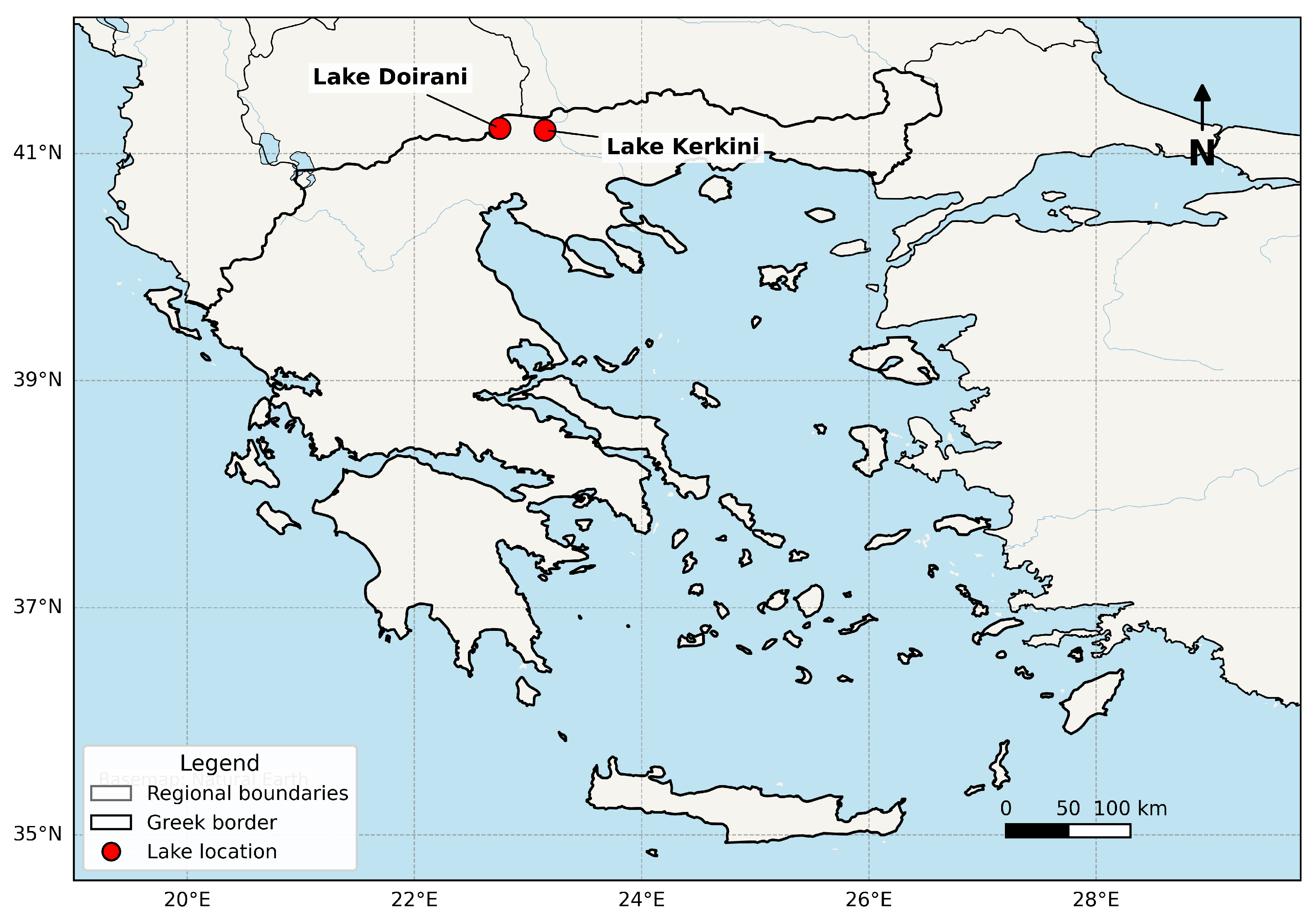
The primary study area for model training and local evaluation is the broader basin of Lake Kerkini in Central Macedonia, Northern Greece (41°13′N, 23°08′E) (Figure 1). Created in 1932 as an artificial reservoir on the Strymon River, the lake’s surface area ranges up to approximately 75 km² depending on the season and water levels. This region was selected due to its highly heterogeneous and dynamic landscape. It is a designated Ramsar Wetland of International Importance and a Natura 2000 site, encompassing a vital aquatic ecosystem, extensive agricultural plains, dense riparian forests and diverse natural vegetation. The co-existence of these distinct land cover types makes it an ideal, yet challenging, environment for training land-cover classification models.

To evaluate regional transferability, a secondary, independent region surrounding Lake Doirani (41°13′N, 22°45′E) was used as an independent regional test site. Lake Doirani is a natural transboundary lake shared between Greece and North Macedonia, covering a total surface area of roughly 43.1 km². Being a relic of the ancient Lake Paionia, it features different morphological characteristics and vegetation patterns compared to Kerkini. Applying the models trained on Kerkini directly to the Doirani basin provides a regional transferability evaluation within a nearby Mediterranean landscape, rather than a broad test of generalization to substantially different geographic or climatic settings.

2.2. Satellite Data Acquisition and Preprocessing

The primary Earth observation data utilized in this study consist of multispectral imagery from the Copernicus Sentinel-2 mission. Data ingestion, cloud-masking and temporal aggregation were executed via the Google Earth Engine (GEE) cloud computing platform, leveraging the COPERNICUS/S2_SR_HARMONIZED Level-2A Surface Reflectance collection.

To ensure the spectral quality of the inputs, an image-level cloud filtering and pixel-level masking procedure was implemented. First, Sentinel-2 scenes with a CLOUDY_PIXEL_PERCENTAGE greater than 20% were excluded. Subsequently, pixel-level masking was performed using the Scene Classification Layer (SCL) of the COPERNICUS/S2_SR_HARMONIZED collection. Specifically, pixels classified as cloud shadows (SCL = 3), medium-probability clouds (SCL = 8), high-probability clouds (SCL = 9), cirrus clouds (SCL = 10) and snow/ice (SCL = 11) were masked out from each individual image prior to seasonal median compositing.

To effectively capture the distinct phenological variations characteristic of land-cover types throughout the year, the cloud-free image time-series was partitioned and aggregated into four distinct seasonal periods using a temporal median reducer:

• Winter: 1 December 2020–28 February 2021;
• Spring: 1 March 2021–31 May 2021;
• Summer: 1 June 2021–31 August 2021;
• Autumn: 1 September 2021–30 November 2021.

The use of four seasonal median composites was selected as a compromise between phenological representation, cloud-robustness and input dimensionality. Seasonal aggregation increases the probability of retaining sufficient cloud-free observations after image-level filtering and pixel-level SCL masking, while still preserving the main annual phenological phases relevant to Mediterranean land-cover discrimination. Monthly composites or full time-series inputs could capture shorter-term crop phenology more explicitly, but they would also increase the dimensionality of the input stack, the number of missing or cloud-contaminated observations and the risk of introducing temporally uneven data availability across seasons. Therefore, four seasonal composites were used to provide a compact and more stable multi-temporal representation suitable for the spatial cross-validation and regional transferability framework adopted in this study.

For each seasonal representative composite, ten core spectral bands were selected: Blue (B2), Green (B3), Red (B4), Vegetation Red Edge (B5, B6, B7), Near-Infrared (B8, B8A) and Short-Wave Infrared (B11, B12). All selected Sentinel-2 bands were exported on a common 10 m spatial grid. The native 20 m bands, namely B5, B6, B7, B8A, B11 and B12, were projected to the 10 m output grid during Google Earth Engine export using the platform’s default nearest-neighbor resampling behavior. Nearest-neighbor resampling was retained to preserve the original pixel values of the native bands and to avoid introducing interpolated reflectance values during export. Nevertheless, because these bands contain continuous reflectance data, this choice may preserve block-like patterns from the native 20 m grid and is therefore acknowledged as a preprocessing limitation. The same output grid and spatial resolution were used for the seasonal composites, spectral indices and WorldCover-derived reference-label layers.

To enhance the discrimination capability of the models regarding vegetation vigor, chlorophyll-sensitive vegetation dynamics, surface moisture and artificial surfaces, four established spectral indices were computed directly within GEE and appended to each seasonal stack [12,13,14,15,16,17]. Spectral indices have been widely used in remote sensing to summarize vegetation condition, water-related surface properties and built-up characteristics from multispectral imagery, while recent Mediterranean drought-monitoring studies further demonstrate their relevance for environmental assessment and climate-adaptation applications [12]. The Normalized Difference Vegetation Index (NDVI), a widely used indicator of vegetation activity and ecological responses to environmental change [13], was calculated as:

$$\mathrm{NDVI}={\displaystyle \frac{B8-B4}{B8+B4}}.$$

(1)

The Normalized Difference Water Index (NDWI), using the green and near-infrared bands to enhance open-water features [14], was calculated as:

$$\mathrm{NDWI}={\displaystyle \frac{B3-B8}{B3+B8}}.$$

(2)

It should be noted that alternative NDWI formulations based on near-infrared and short-wave infrared wavelengths have also been proposed for vegetation liquid-water monitoring [15]; however, the present study uses the green–near-infrared formulation because the target land-cover scheme includes permanent surface water bodies.

The Normalized Difference Built-up Index (NDBI), commonly used for enhancing built-up land from multispectral imagery [16], was calculated as:

$$\mathrm{NDBI}={\displaystyle \frac{B11-B8}{B11+B8}}.$$

(3)

The Normalized Difference Red Edge Index (NDRE), which exploits the sensitivity of red-edge and near-infrared reflectance to vegetation chlorophyll-related properties [17], was calculated as:

$$\mathrm{NDRE}={\displaystyle \frac{B8-B5}{B8+B5}}.$$

(4)

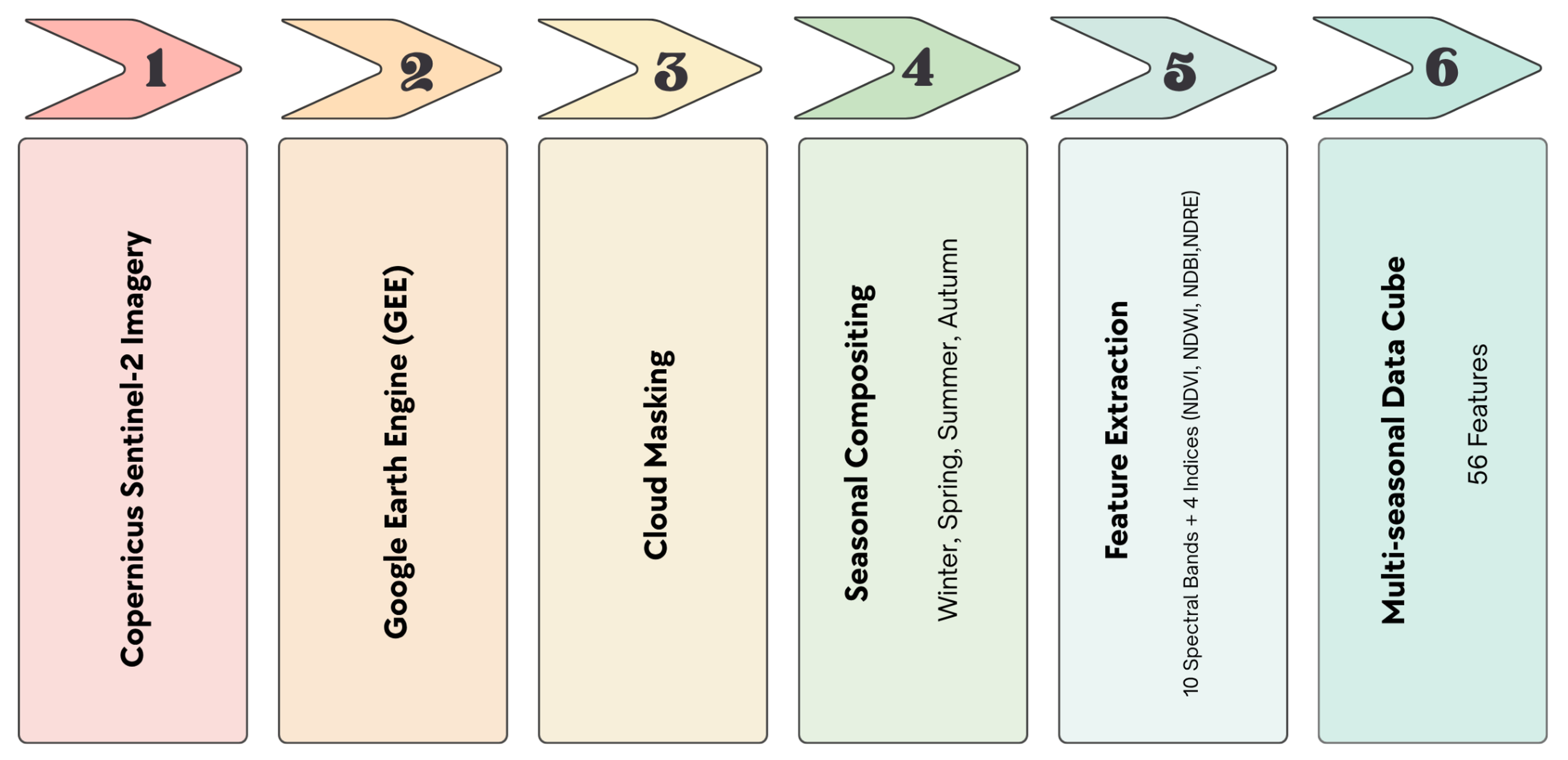
Finally, the individual seasonal composites and their respective indices were concatenated into a single multi-band image. This comprehensive multi-dimensional data cube, comprising 56 structural features (14 variables × 4 seasons), was clipped to the study area geometries and exported at a 10 m spatial resolution to serve as the definitive input for the deep learning workflows (Figure 2).

2.3. ESA WorldCover-Derived Reference Labels

The reference labels used for model training, local spatial cross-validation and regional transferability evaluation were derived from the European Space Agency (ESA) WorldCover 2021 product. The ESA WorldCover dataset provides a global land cover map for the reference year 2021 at a high spatial resolution of 10 m, generated through the synergistic processing of Sentinel-1 Synthetic Aperture Radar (SAR) and Sentinel-2 optical data. In this study, ESA WorldCover was used as a standardized, spatially explicit reference-label source rather than as independent field-based ground truth.

To adapt this global classification scheme to the specific environmental, phenological and geographical characteristics of the Mediterranean study basins, the original WorldCover classification categories were systematically reclassified and aggregated into five consolidated primary land-cover classes:

• Water (Class 1): Encompasses all permanent open surface water bodies, including natural lakes, river networks and artificial reservoirs, corresponding directly to the original ESA WorldCover class 80.
• Cropland (Class 2): Includes actively managed agricultural lands, intensively cultivated fields and seasonal crop zones, corresponding to the original ESA WorldCover class 40.
• Forest (Class 3): Comprises dense and sparse tree cover formations, including evergreen, deciduous, coniferous and mixed forest environments, corresponding to the original ESA WorldCover class 10.
• Low/Natural Vegetation (Class 4): A synthesized broad class aggregating natural and semi-natural low-stature vegetation types, including shrublands, grasslands, herbaceous wetlands and transitional vegetation zones, corresponding to the original ESA WorldCover classes 20, 30, 90, 95 and 100.
• Built-up (Class 5): Covers artificial surfaces, urban structures, building complexes, consolidated transport infrastructure and non-vegetated engineered surfaces, corresponding to the original ESA WorldCover class 50.

The adopted five-class scheme was designed to support broad operational land-cover mapping rather than fine ecological habitat discrimination. Therefore, some target classes intentionally aggregate multiple original ESA WorldCover categories. This is particularly important for the Low/Natural Vegetation class, which combines shrubland, grassland, herbaceous wetland and transitional vegetation categories. Although this aggregation reduces label fragmentation and produces a more stable class structure for regional model training, it also reduces ecological specificity. These subcategories may show different phenological trajectories, canopy structures and moisture conditions across seasons, increasing within-class spectral variability and potentially affecting class separability.

Original ESA WorldCover categories that were absent or had very limited spatial representation within the target catchments were omitted from the reclassification procedure. Specifically, the Bare/Sparse Vegetation class (original ESA WorldCover class 60) was masked out because it was not sufficiently represented in the study areas. This masking step was applied to reduce label ambiguity and avoid introducing poorly represented classes during model training and evaluation.

The final remapped 10 m WorldCover-derived reference-label layers for both the Kerkini and Doirani basins were spatially co-registered and aligned with the preprocessed multi-seasonal Sentinel-2 feature stacks. This ensured an exact pixel-to-pixel geometric correspondence across the entire dataset, which is a fundamental prerequisite for accurate spatial patch extraction and neural network training. Consequently, the labels used in this study should be interpreted as ESA WorldCover-derived reference labels, or pseudo-reference labels, rather than independently verified ground-truth observations.

2.4. Deep Learning Architectures

To thoroughly evaluate the optimal approach for multi-seasonal land-cover classification, this study implements and compares four distinct deep learning architectures. These models were carefully selected to represent fundamentally different paradigms in computer vision, ranging from traditional local convolutions to modern global attention mechanisms.

• Convolutional Neural Network (CNN): Serving as the robust baseline, a standard multi-layer 2D CNN was implemented. CNNs are highly effective at automatically extracting hierarchical spatial and spectral features through localized convolutional kernels. They represent the traditional powerhouse for patch-based satellite image classification due to their inherent translational equivariance and spatial feature preservation capabilities.
• UNet++: Representing advanced semantic segmentation models, UNet++ is a powerful evolution of the classic encoder–decoder U-Net architecture. Its distinguishing feature is the integration of nested, dense skip connections [5]. These dense connections effectively bridge the semantic gap between the encoder’s high-resolution spatial feature maps and the decoder’s high-level semantic features. This architecture is particularly relevant to land-cover classification tasks, as it allows the network to retain fine-grained spatial details needed for delineating complex boundaries, such as highly fragmented agricultural plots or narrow riparian zones.
• ConvNeXt: Introduced to modernize standard ResNet-like architectures, ConvNeXt is a pure convolutional model constructed with design choices heavily inspired by the successes of Vision Transformers [9]. By incorporating larger kernel sizes (e.g., $7\times 7$), inverted bottlenecks and depthwise convolutions, ConvNeXt aims to deliver the computational efficiency and inductive bias of traditional convolutions while successfully matching the representational capacity, robustness and scalability of Transformers.
• Vision Transformer (ViT): Departing entirely from convolutions, the ViT architecture relies exclusively on the self-attention mechanism [7]. It treats the input multi-seasonal patches as a sequence of flattened, non-overlapping tokens, applying multi-head self-attention to capture global context and long-range dependencies across the entire input patch. While highly expressive, ViTs inherently lack the geometric priors (such as translational equivariance) of CNNs, testing the adaptability of pure attention mechanisms to localized, multi-band remote sensing data.

2.5. Spatial Cross-Validation Strategy

Evaluating land-cover classification models using standard random training–test splits can lead to severely optimistic performance estimates. This occurs due to spatial autocorrelation, i.e., the tendency of geographically neighboring pixels to share similar spectral signatures, topographical characteristics and environmental conditions. When adjacent or nearby pixels are randomly distributed between training and test sets, the assumption of sample independence is weakened and the model may partly learn local spatial patterns rather than features that generalize to unseen geographic areas.

To obtain a more robust and spatially independent assessment, the dataset was partitioned using a strict spatial cross-validation strategy. As emphasized in recent literature, spatial split strategies are essential for mitigating the adverse effects of spatial autocorrelation and preventing the artificial inflation of accuracy metrics in remote sensing classification tasks [18,19].

In the proposed approach, each outer fold used a geographically contiguous rectangular region as the held-out test area. The four outer test regions were selected as non-overlapping spatial blocks. Instead of using unrestricted random pixel sampling, candidate test blocks were generated and screened through a class-aware spatial-block procedure. Candidate rectangular blocks of comparable geometry were examined in different parts of the Lake Kerkini basin and were retained only when they were non-overlapping, could be surrounded by the 300 m exclusion buffer and provided sufficient representation of all target land-cover classes. This screening step was applied to avoid misleading evaluation folds dominated almost entirely by a single easy-to-classify class, such as water or cropland, which could artificially inflate accuracy estimates and weaken the interpretation of model generalization.

Table 1. Class support, equivalent area and relative class proportion in the four Lake Kerkini spatial test folds and in the independent Lake Doirani regional test area. Areas were calculated from the 10 m WorldCover-derived reference-label grid.

Evaluation Region	Class	Pixels	Area (km2)	Proportion (%)
Fold 1	Water	11,270	1.13	7.86
Fold 1	Cropland	30,030	3.00	20.94
Fold 1	Forest	38,858	3.89	27.10
Fold 1	Low/Natural Vegetation	57,621	5.76	40.18
Fold 1	Built-up	5621	0.56	3.92
Fold 2	Water	6714	0.67	4.09
Fold 2	Cropland	78,805	7.88	48.06
Fold 2	Forest	35,689	3.57	21.76
Fold 2	Low/Natural Vegetation	31,898	3.19	19.45
Fold 2	Built-up	10,880	1.09	6.63
Fold 3	Water	12,453	1.25	7.32
Fold 3	Cropland	48,994	4.90	28.78
Fold 3	Forest	33,962	3.40	19.95
Fold 3	Low/Natural Vegetation	65,516	6.55	38.49
Fold 3	Built-up	9294	0.93	5.46
Fold 4	Water	13,949	1.39	8.84
Fold 4	Cropland	96,478	9.65	61.17
Fold 4	Forest	18,674	1.87	11.84
Fold 4	Low/Natural Vegetation	16,192	1.62	10.27
Fold 4	Built-up	12,423	1.24	7.88
Lake Doirani	Water	551,484	55.15	21.69
Lake Doirani	Cropland	659,136	65.91	25.93
Lake Doirani	Forest	823,616	82.36	32.40
Lake Doirani	Low/Natural Vegetation	448,875	44.89	17.66
Lake Doirani	Built-up	58,921	5.89	2.32

reports the class support, equivalent area and relative class proportion of the WorldCover-derived reference labels in each held-out Lake Kerkini spatial test fold. For completeness, the same information is also reported for the independent Lake Doirani regional test area used later for regional transferability evaluation. Because all reference-label pixels were aligned to the 10 m Sentinel-2 grid, each pixel corresponded to 100 m², or 0.0001 km².

The final four Lake Kerkini test blocks contained all five target classes, confirming that the class-aware screening procedure produced multi-class test regions rather than single-class or near-single-class evaluation areas. However, the folds were not forced to be class-balanced, because the objective was to preserve realistic spatial test regions while avoiding extreme class dominance. Therefore, the reported evaluation should be interpreted as spatially independent and class-representative, but not as a fully stratified or perfectly balanced sampling design.

To strictly enforce spatial separation, buffer “dead zones” were applied around each test region. The buffer width was set to 30 pixels, corresponding to 300 m at the 10 m spatial resolution of the Sentinel-2 feature stack. This distance was defined as twice the radius of the largest patch size considered in the hyperparameter search, namely a 31 × 31 pixel patch. Pixels within the test-region buffer zones were excluded from the training and validation subsets, ensuring that samples immediately adjacent to the test area could not be used during model development. This design reduced the risk of spatial leakage between the training/validation and test subsets.

After the test region and its buffer were excluded, the remaining valid pixels were used to define spatially separated training and validation subsets. An additional 30-pixel buffer was also applied around the validation area during model selection to further reduce spatial leakage. Pixels located inside this validation buffer were excluded from the training subset.

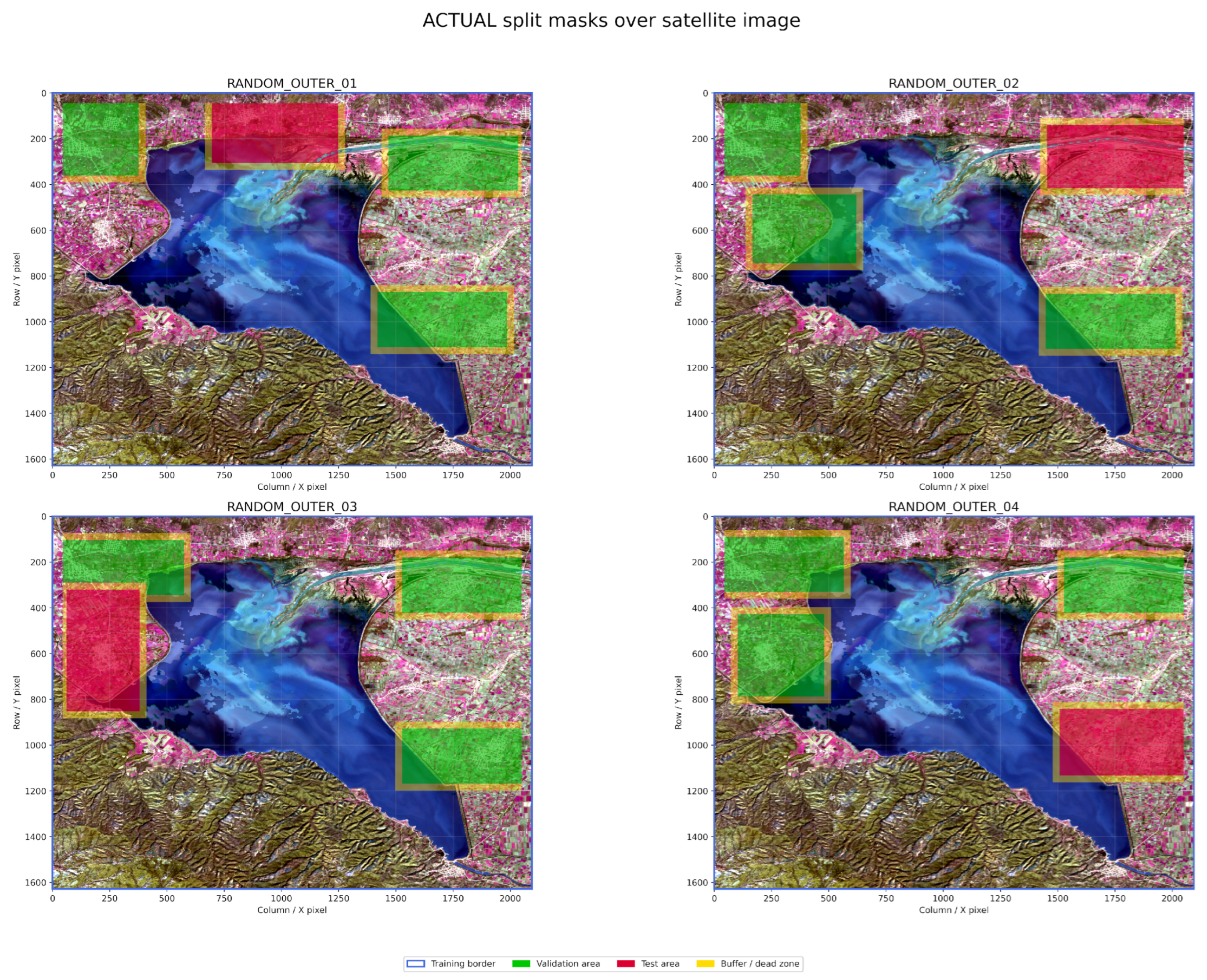
As illustrated in Figure 3, each outer fold was defined by spatial masks separating the held-out test region, the validation region, the eligible training region and the excluded buffer/dead zones. The red areas correspond to the spatially contiguous test regions, the green areas indicate the validation regions, the blue areas represent the remaining eligible training regions and the yellow areas denote the buffer/dead zones used to enforce spatial separation between neighboring subsets.

Overall, this procedure ensured that model evaluation was conducted on geographically independent out-of-sample regions while maintaining adequate representation of the target classes across the cross-validation folds. Because spatial-block validation can depend on the location and composition of the selected test regions, the four folds were distributed across different parts of the study area, used comparable block geometry and were evaluated separately before aggregation. This design was intended to reduce dependence on any single favorable test location while retaining a more conservative and spatially realistic assessment than random pixel-based validation.

2.6. Experimental Setup and Training Parameters

All experiments were implemented in Python 3 using TensorFlow 2.20.0 and its integrated Keras API. Each model was trained as a patch-based classifier, where the input consisted of a multispectral Sentinel-2 patch and the target label corresponded to the central pixel of that patch. The classification task involved five target land-cover classes. Prior to training, the input features were standardized using band-wise mean and standard deviation values computed only from the training area of each fold, preventing information from the validation or test regions from being introduced during preprocessing.

Hyperparameter optimization (HPO) was conducted using a leakage-safe global spatial validation scheme. Before model selection, the outer test regions and their corresponding buffer zones were excluded from the hyperparameter selection process. The remaining spatially safe development area was divided into four spatial validation subfolds. For each candidate configuration, balanced training and validation subsets were extracted, using up to 3000 training samples per class and 1000 validation samples per class, respectively.

A compact set of eight predefined candidate configurations was evaluated for all architectures to ensure a fair comparison. These configurations were designed to cover different levels of spatial context, model capacity, regularization strength and optimization behavior, while keeping the computational cost feasible under the spatial validation protocol. Specifically, the configurations varied the patch size, number of convolutional filters, dense layer size, dropout rate and learning rate, as shown in

Table 2. Predefined candidate hyperparameter configurations evaluated under the spatial validation scheme. Patch size denotes the side length of the spatial input window in pixels. The same set of configurations was used for all tested architectures.

Trial	Patch Size (Pixels per Side)	Filters 1 (Kernels)	Filters 2 (Kernels)	Dense Units (Neurons)	Dropout Rate (%)	Learning Rate (η)
1	19	32	64	256	30	$3\times {10}^{-4}$
2	23	48	96	384	30	$2\times {10}^{-4}$
3	27	64	128	512	40	$1\times {10}^{-4}$
4	23	64	96	256	20	$3\times {10}^{-4}$
5	19	48	128	384	30	$2\times {10}^{-4}$
6	27	48	96	512	20	$2\times {10}^{-4}$
7	31	32	96	256	40	$1\times {10}^{-4}$
8	23	32	128	512	30	$3\times {10}^{-4}$

.

During hyperparameter optimization, each candidate model was trained with a maximum epoch budget of up to 50 epochs. Early stopping was applied based on the validation loss with a patience of four epochs and a minimum improvement threshold of ${10}^{-4}$. Training was terminated when the validation loss did not improve for four consecutive epochs, following the validation-based early stopping principle described by Prechelt [20]. The model weights corresponding to the lowest validation loss were restored after early stopping. This was implemented using the Keras EarlyStopping option restore_best_weights=True [21]. Model selection was based on the mean validation Macro-F1 score across the four spatial HPO subfolds. Macro-F1 was selected as the optimization criterion because it provides a more balanced assessment than overall accuracy when class frequencies are uneven. The best-performing configuration selected for each architecture is reported in

Table 3. Best hyperparameter configuration selected for each architecture based on the mean Macro-F1 score across the four spatial HPO validation subfolds.

Architecture	Trial	Patch Size	Filters 1	Filters 2	Dense Units	Dropout	Learning Rate	HPO Macro-F1
CNN	5	19	48	128	384	0.30	$2\times {10}^{-4}$	$0.8394\pm 0.0238$
UNet++	1	19	32	64	256	0.30	$3\times {10}^{-4}$	$0.8366\pm 0.0207$
ConvNeXt	5	19	48	128	384	0.30	$2\times {10}^{-4}$	$0.8537\pm 0.0209$
ViT	5	19	48	128	384	0.30	$2\times {10}^{-4}$	$0.7817\pm 0.0297$

.

To provide a clearer comparison of model capacity and training setup, the main architectural characteristics of the final models are summarized in

Table 4. Main architectural characteristics of the evaluated models. Parameter counts refer to the final fold-specific models; the architecture was identical across the four outer folds within each model family.

Architecture	Input Shape	Trainable Parameters	Main Structure and Pretraining
CNN	$19\times 19\times 56$	476,741	3 Conv2D blocks followed by a dense classifier; no pretraining
UNet++	$19\times 19\times 56$	544,773	3-level nested encoder–decoder with dense skip connections; no pretraining
ConvNeXt	$19\times 19\times 56$	1,679,093	ConvNeXt-style architecture with 6 depthwise-convolution blocks; no pretraining
ViT	$19\times 19\times 56$	561,669	3 transformer blocks with embedding dimension 128 and 4 attention heads; no pretraining

. The four fold-specific models had identical architecture within each model family. All models were trained from scratch without ImageNet pretraining, remote-sensing pretraining or other external pretraining.

The evaluated architectures were not constrained to have identical parameter counts. The purpose of the comparison was to assess which established model family performed most robustly under the same input-feature set, spatial validation protocol, sampling strategy, optimizer, loss function and hyperparameter-selection procedure. Thus, the experiment should be interpreted as a controlled same-protocol evaluation for the present Sentinel-2 land-cover case study, rather than as a strictly parameter-matched theoretical benchmark. This distinction is important for interpreting the ViT results, since transformer-based models often benefit from large-scale pretraining or substantially larger training datasets.

After selecting the best configuration for each architecture, final training was performed independently for each of the four outer spatial folds. For each fold, up to 15,000 training samples per class and 4000 validation samples per class were extracted from the spatially separated training and validation areas. All models were optimized using the Adam optimizer with decoupled weight decay (AdamW) and sparse categorical cross-entropy loss. The final fold-specific models were trained with a maximum epoch budget of up to 50 epochs. Early stopping was applied based on the validation loss with a patience of four epochs and a minimum improvement threshold of ${10}^{-4}$. This strategy was used as a regularization mechanism to limit unnecessary training once validation performance stopped improving [22]. The same best-weight restoration setting was applied after early stopping. Learning-rate reduction on plateau was also applied based on the validation loss to reduce overfitting during training. Final evaluation was carried out on all valid pixels within the corresponding spatial test region of each outer fold.

Computational cost was recorded for the hyperparameter search, final training and test inference stages using an NVIDIA A100 graphics processing unit (GPU; NVIDIA Corporation, Santa Clara, CA, USA), accessed through the Google Colaboratory environment. Runtime values are reported in Section 3.

The main experimental and training parameters are summarized in

Table 5. Main experimental and training parameters used in the spatial cross-validation experiments.

Parameter	Value
Framework	TensorFlow/Keras
Computational environment	NVIDIA A100 GPU environment for all experiments
Runtime measurements	HPO search, final training and test inference
Optimizer	AdamW
Loss function	Sparse categorical cross-entropy
Model selection metric	Mean validation Macro-F1
Evaluation metrics	Overall accuracy and Macro-F1 score
Number of candidate configurations	8
Spatial HPO validation subfolds	4
HPO training samples	Up to 3000 samples per class
HPO validation samples	Up to 1000 samples per class
HPO maximum epoch budget	Up to 50 epochs
HPO early stopping	Validation-loss patience of 4 epochs, minimum delta ${10}^{-4}$
HPO best-weight restoration	Enabled using the lowest validation loss
Final training samples	Up to 15,000 samples per class
Final validation samples	Up to 4000 samples per class
Final maximum epoch budget	Up to 50 epochs
Final early stopping	Validation-loss patience of 4 epochs, minimum delta ${10}^{-4}$
Final best-weight restoration	Enabled using the lowest validation loss
Learning-rate scheduling	ReduceLROnPlateau based on validation loss
Training regularization	Early stopping, best-weight restoration and learning-rate reduction on plateau
Normalization	Fold-specific band-wise mean and standard deviation
Randomness control	Global seed with stage-specific seeds for spatial splitting and sampling

.

To improve reproducibility, a global random seed was used together with stage-specific seeds for the main stochastic components of the workflow, including spatial split generation, hyperparameter optimization sampling and final train–validation sampling. This ensured that the partitioning and sampling procedures were deterministic while still allowing independent randomization across different experimental stages.

Overall, this experimental design ensured that all architectures were compared under the same spatial validation protocol, the same candidate hyperparameter configurations and the same final outer-fold evaluation procedure. This allowed performance differences to be attributed primarily to the model architectures rather than to differences in data partitioning, sampling or hyperparameter search conditions. However, because the architectures differ in design and parameter count, the comparison should be interpreted as a controlled same-protocol evaluation rather than as a strictly parameter-matched benchmark.

2.7. Feature Importance Analysis

Deep learning models can achieve high predictive performance in remote sensing applications, but their internal decision-making process is often difficult to interpret, which limits their scientific transparency and operational trustworthiness [23,24,25]. This is particularly important in land-cover classification, where understanding which spectral or seasonal input channels drive model predictions can provide additional insight into the learned class-discrimination patterns and help assess whether the model relies on meaningful remote sensing information rather than spurious correlations. Feature and band importance analysis has long been considered valuable in remote sensing because it supports model interpretation, identifies influential spectral regions and helps understand the contribution of different input variables to classification performance [26,27].

To interpret the behavior of the trained models, a feature importance analysis was conducted using an independent external evaluation area that was not used during model training, hyperparameter optimization, or spatial cross-validation. The analysis was performed using the four fold-specific models of each architecture, together with their corresponding fold-specific normalization statistics. This ensured that each model was evaluated under the same preprocessing conditions used during its original training. Predictions were obtained in an ensemble setting by averaging the softmax probability vectors produced by the four fold-specific models.

A balanced set of image patches was extracted from the external evaluation area, using up to 300 samples per land-cover class. Each sample consisted of a multispectral patch centered on a labeled pixel. The ensemble prediction for each patch was first computed and used as the baseline prediction for the attribution analysis. Feature importance was then assessed at the input-channel level using two complementary attribution approaches: perturbation-based occlusion and Gradient × Input. The main components of the feature importance workflow are summarized in

Table 6. Components of the feature importance analysis.

Component	Purpose	Output
Ensemble occlusion	Measures the effect of masking each input channel	Mean probability drop and prediction flip rate
Gradient × Input	Estimates gradient-based input-channel sensitivity	Channel-level gradient attribution scores
Class-wise attribution	Evaluates importance separately for each reference class	Class-specific importance rankings
Fold-wise stability	Assesses consistency across independently trained folds	Spearman rank correlations and fold-wise variability
Consensus ranking	Combines perturbation-based and gradient-based rankings	Final ranked list of influential input channels
Gradient-weighted Class Activation Mapping (Grad-CAM) visualization	Provides qualitative spatial explanations within selected patches	Heatmaps for correct and incorrect predictions

.

For the perturbation-based analysis, a zero-masking occlusion strategy was applied. Occlusion-based sensitivity analysis is commonly used to assess how model predictions change when specific parts of the input are removed or altered [28]. In this study, each input channel was masked individually by setting its raw values to zero before applying the corresponding fold-specific normalization. The modified patches were then passed through the ensemble and the resulting probabilities were compared with the original baseline predictions. For each input channel, two quantities were computed: the mean decrease in the probability of the original predicted class and the prediction flip rate. The mean probability drop quantified how strongly the ensemble confidence decreased after masking a given input channel, while the flip rate measured how often the predicted class changed after the occlusion. Channels producing larger probability drops or higher flip rates were considered more influential for the model predictions.

It should be noted that zero-masking was used here as a post-hoc channel-occlusion sensitivity analysis, rather than as a retraining-based feature-ablation experiment or as a physically exact simulation of missing or naturally occurring spectral observations. Since the raw values of an input channel are set to zero prior to fold-specific normalization, the resulting perturbed samples may not always correspond to physically realistic Sentinel-2 reflectance conditions. Therefore, the occlusion scores were interpreted as measures of model sensitivity to channel removal under a controlled perturbation setting. To reduce dependence on this single perturbation mechanism, the occlusion analysis was complemented with Gradient × Input attribution, class-wise attribution and fold-wise stability assessment.

In addition to occlusion, a Gradient × Input attribution method was used to obtain a complementary gradient-based estimate of input-channel importance. Gradient-based saliency methods estimate the sensitivity of the model output with respect to the input features and have been widely used to visualize and interpret deep neural network predictions [29,30]. For each sample, gradients of the predicted class probability were computed with respect to the normalized input patch. These gradients were multiplied by the corresponding input values and the absolute attribution values were averaged across samples, spatial patch dimensions and fold-specific models. This produced a single importance score for each input channel. Since occlusion and Gradient × Input capture different aspects of model sensitivity, both methods were retained rather than relying on a single attribution measure.

The analysis was also repeated separately for each reference land-cover class. In the class-wise analysis, samples were grouped according to their reference label and input-channel importance was computed independently for each class. This allowed the identification of channels that were particularly influential for specific land-cover categories, rather than only for the global ensemble behavior. For the occlusion-based class-wise analysis, importance was measured as the change in the model’s original prediction confidence within each reference-class group. For the gradient-based class-wise analysis, attribution was computed with respect to the corresponding class output.

To evaluate the stability of the feature importance results, the attribution analysis was also performed independently for each of the four fold-specific models. For each fold, input-channel rankings were generated using both occlusion and Gradient × Input. The agreement between fold-specific rankings was then quantified using Spearman rank correlation. This step was included to assess whether the most influential input channels were consistently identified across independently trained spatial folds, rather than being driven by a single model instance.

A consensus importance ranking was then produced by combining the global ensemble occlusion ranking and the global ensemble Gradient × Input ranking. For each input channel, ranks from the two attribution methods were averaged to obtain a final consensus rank. Fold-wise variability was additionally quantified through a stability score based on the standard deviation of fold-specific attribution scores and was reported as a diagnostic measure of ranking consistency. Therefore, input channels ranked highly by both attribution methods and showing low variability across folds were considered the most stable attribution features within the tested models.

Finally, Grad-CAM visualizations were generated as qualitative spatial explanations for selected correct and incorrect predictions. Grad-CAM uses gradients flowing into convolutional feature maps to produce class-discriminative localization heatmaps, making it useful for visualizing the spatial regions that contribute to a model prediction [31]. In this study, Grad-CAM was computed for each fold-specific model and then averaged across folds to obtain an ensemble-level spatial explanation. These heatmaps were used only to visualize which spatial regions within the input patch contributed most strongly to selected predictions. They were not used as input-channel importance measures.

Overall, the feature importance analysis was designed as a model-attribution procedure rather than as a causal analysis. The resulting rankings identify the input channels and patch regions that most strongly influenced the trained models’ predictions, but they should not be interpreted as proof of causal relationships between individual spectral bands and land-cover classes. In particular, high attribution scores indicate that the trained networks relied strongly on specific spectral-seasonal channels during prediction, not that these channels are uniquely or causally responsible for the physical separability of land-cover categories. This distinction is important because attribution methods explain model behavior, not necessarily the underlying physical or ecological processes that generated the observed land-cover patterns [25,30].

In addition, because several derived indices are deterministic functions of raw Sentinel-2 bands included in the same input stack, the attribution scores should be interpreted under strong feature collinearity. Under such conditions, importance may be distributed unevenly between raw bands and derived indices and low attribution for an index does not necessarily indicate that the corresponding spectral relationship is irrelevant.

No separate retraining experiment was conducted in which spectral indices were removed from the input stack. Therefore, the present analysis should be interpreted as an attribution-based assessment within the full-feature configuration, not as direct causal evidence of the incremental performance contribution of the indices. A dedicated with- and without-indices ablation experiment would be required to quantify whether the derived indices improve, reduce, or leave unchanged the predictive performance of each architecture. Accordingly, the lower attribution scores observed for NDVI, NDWI, NDBI and NDRE are interpreted only as evidence that these indices provided limited additional model attribution when their constituent raw Sentinel-2 bands were simultaneously available.

3. Experimental Results

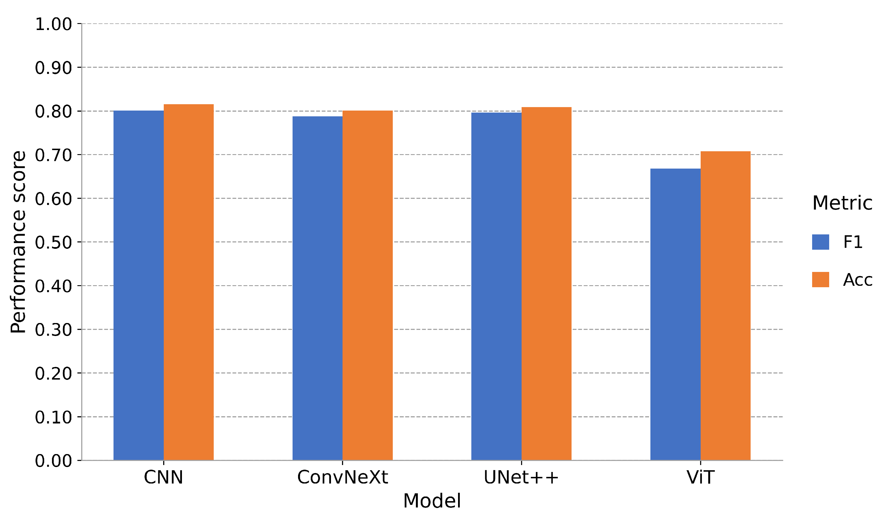
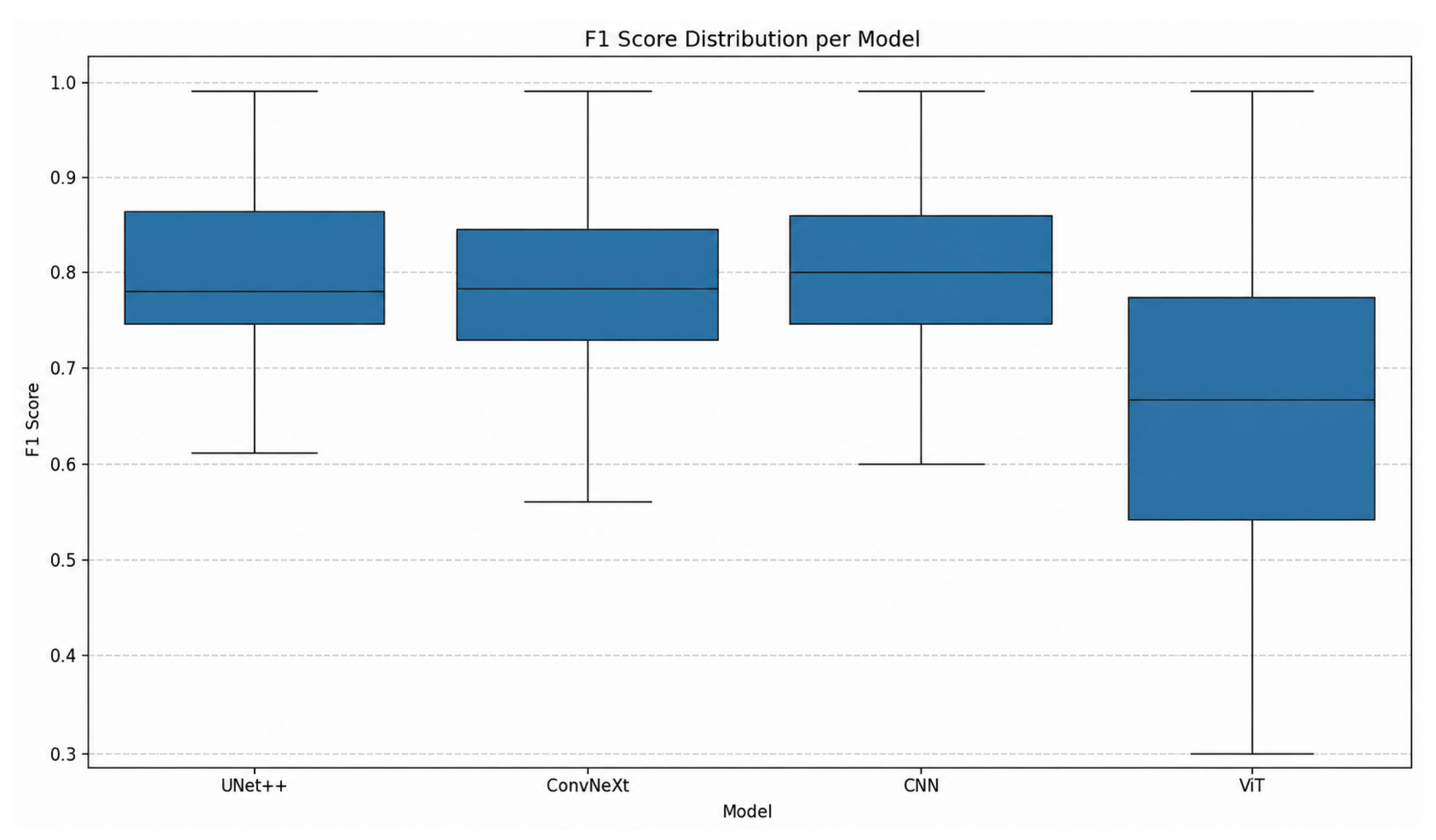
The quantitative performance of the four deep learning architectures was assessed under the strict 4-Fold Spatial Cross-Validation protocol described in Section 2.5. Figure 4 summarizes the mean Overall Accuracy (OA) and macro-averaged F1-score (Macro-F1) obtained across the four spatially independent test folds. The fold-level distribution of Macro-F1 scores across all land-cover classes is additionally visualized through the box-plot in Figure 5, which captures both central tendency and inter-fold variability for each model.

The CNN achieved the highest fold-mean aggregate performance, reaching a mean OA of 81.53% and a mean Macro-F1 of 80.09%. UNet++ followed very closely, recording a mean OA of 80.84% and a Macro-F1 of 79.65%, while also showing the lowest standard deviation in Macro-F1 across the four folds. ConvNeXt attained slightly lower but still competitive metrics (OA = 80.09%, Macro-F1 = 78.76%).

In contrast, the tested Vision Transformer (ViT) configuration recorded lower performance, with a mean OA of approximately 70.74% and a Macro-F1 of 66.79%. This result indicates that, under the present training-data regime, no-pretraining setup and spatial validation protocol, the tested ViT configuration was less effective than the convolutional architectures.

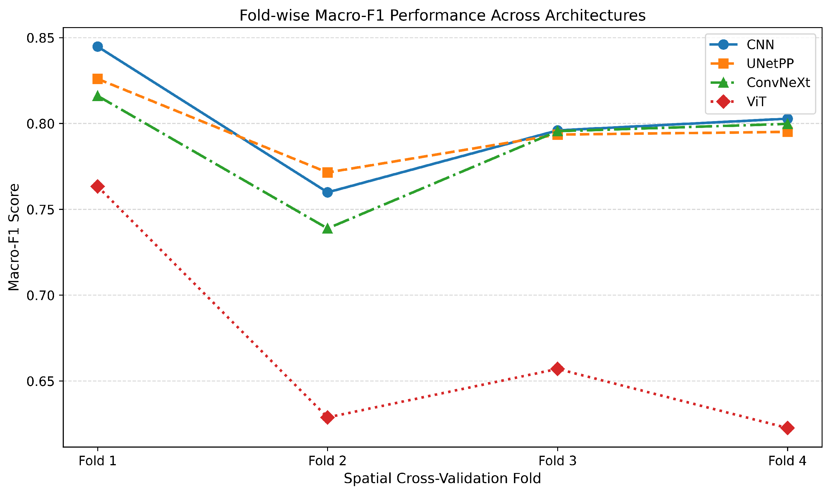
The fold-level Macro-F1 scores further illustrate the relative stability of the convolutional architectures. The CNN recorded fold-specific Macro-F1 values of 0.845, 0.760, 0.796 and 0.803 across Folds 1–4, respectively. UNet++ obtained scores of 0.826, 0.771, 0.794 and 0.795. ConvNeXt produced 0.816, 0.739, 0.796 and 0.800. The ViT exhibited the highest inter-fold variability, with Macro-F1 scores of 0.763, 0.629, 0.657 and 0.623, suggesting that the purely attention-based approach is less consistent across the diverse spatial configurations of the four outer folds. A similar pattern is visible in the per-class F1-score distributions shown in Figure 5, where the ViT displays a lower median and a substantially wider spread than the three convolutional models.

3.1. Computational Cost and Training Behavior

To complement the accuracy-based evaluation, the computational cost of each architecture was also assessed.

Table 7. Computational cost of the evaluated architectures. The number of HPO trials refers to the candidate configurations evaluated during model selection. Hyperparameter-search time refers to the complete model-selection stage for each architecture. Final training time is reported per outer fold and as the total time across the four outer folds. Test inference time refers to full-pixel prediction over the spatial test regions.

Architecture	HPO Trials	HPO Search Time	Final Training Time	Total Final Training Time	Test Inference Time
CNN	8	31.53 min	$1.55\pm 0.44$ min/fold	6.21 min	$78.22\pm 4.09$ s/fold
UNet++	8	48.57 min	$1.43\pm 0.13$ min/fold	5.72 min	$84.74\pm 4.38$ s/fold
ConvNeXt	8	88.85 min	$3.50\pm 0.51$ min/fold	13.99 min	$100.37\pm 11.76$ s/fold
ViT	8	51.81 min	$2.04\pm 0.94$ min/fold	8.16 min	$83.02\pm 4.01$ s/fold

reports the hyperparameter-search time, final training time and test inference time for the evaluated models. All architectures were evaluated using the same NVIDIA A100 GPU environment. The number of HPO trials corresponds to the eight predefined candidate configurations used during model selection.

The runtime comparison shows that the CNN required the shortest hyperparameter-search time, whereas ConvNeXt was the most computationally demanding architecture during model selection and final training. UNet++ achieved the lowest total final training time despite its encoder–decoder structure. Test inference times were broadly comparable across the evaluated architectures, although ConvNeXt required the longest average inference time. These results show that the tested architectures differed not only in classification performance but also in computational cost.

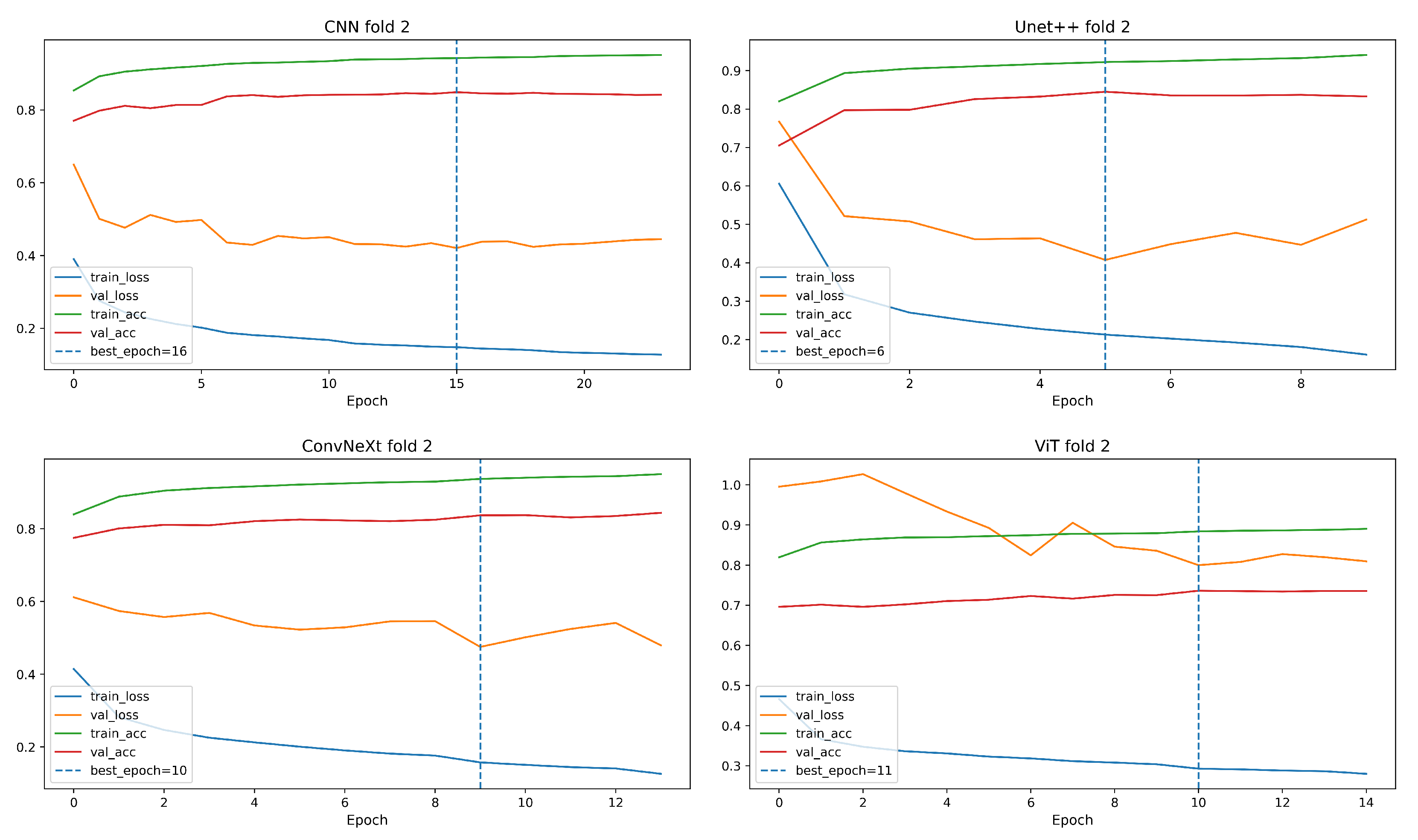
Representative training and validation loss curves are used to inspect the training behavior of the selected configurations. These curves are useful for verifying that the 50-epoch setting acted as a maximum training budget rather than as a fixed training duration. In practice, the effective number of training epochs was determined by validation-loss early stopping, allowing training to stop when no further validation improvement was observed. This strategy was applied to reduce the risk of overfitting and to ensure that each model stopped at an appropriate point according to its generalization behavior rather than simply training for the maximum number of epochs.

The behavior of the training and validation curves is also consistent with the strict spatial validation design used in this study. The validation data were spatially independent from the training data and were not previously seen by the models during parameter optimization. In addition, a spatial buffer was applied between training and validation samples, following the same rationale as in the test-area evaluation, in order to minimize spatial leakage. Therefore, differences between training and validation losses are expected and should be interpreted in the context of a deliberately strict validation protocol rather than as evidence of an unreliable training process.

Figure 6 presents representative training and validation loss curves from fold 2 for the selected model configurations. These curves were included as indicative examples of the training behavior, rather than as an exhaustive presentation of all training runs. Presenting the complete set of curves for all architectures and all outer folds would require sixteen separate plots, since four architectures were evaluated across four folds. Therefore, the representative fold was selected to document the effect of early stopping and the general convergence behavior without overloading the results section with repetitive figures.

3.2. Class-Wise Confusion Structure in Lake Kerkini (Test Area)

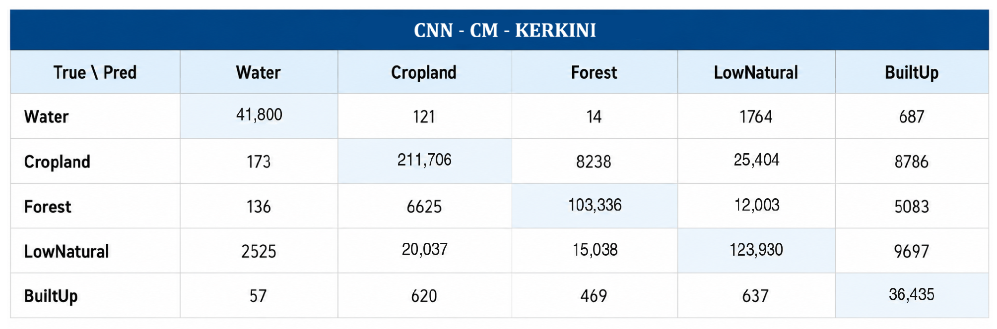
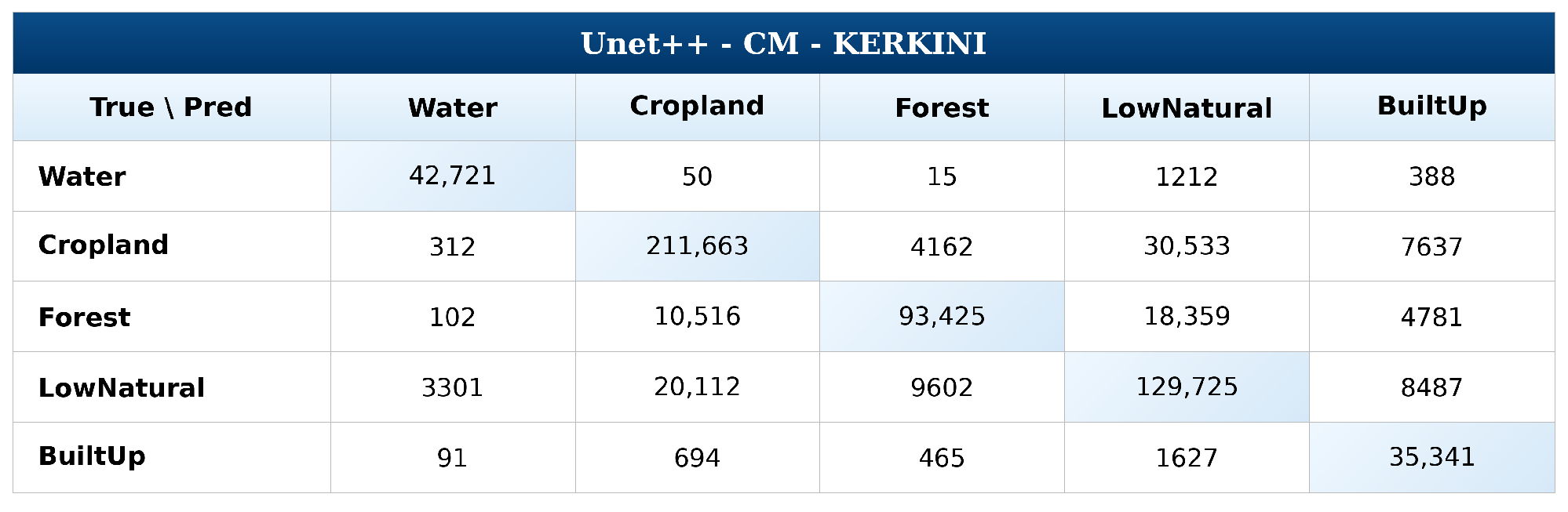
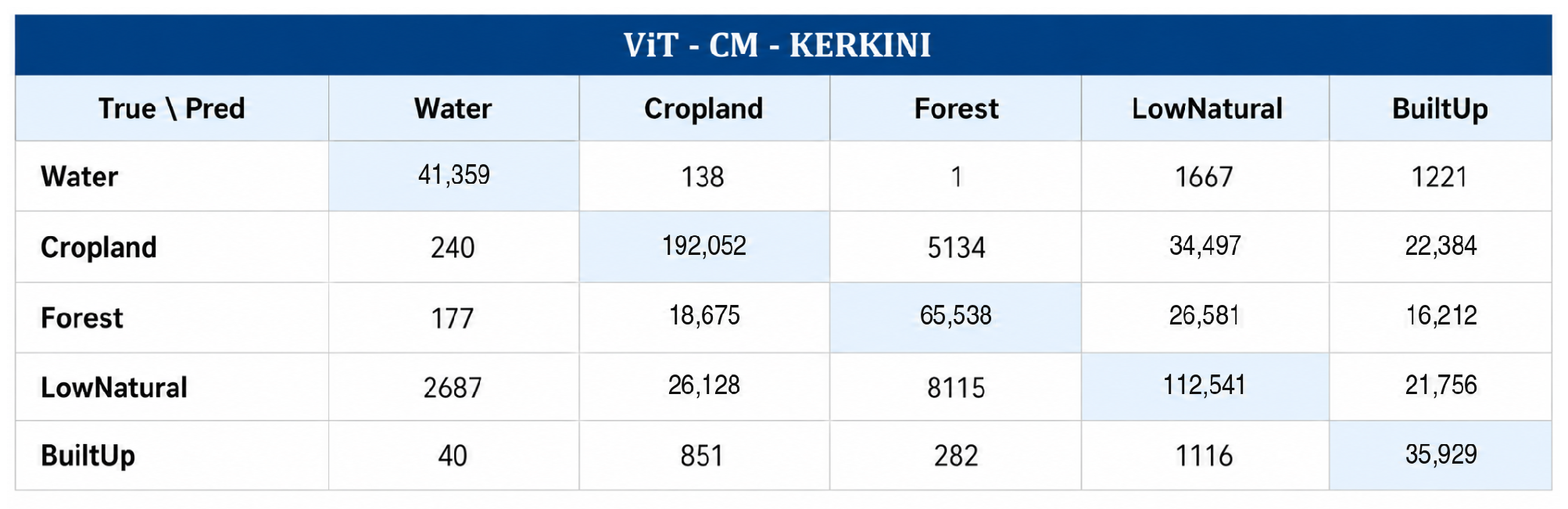
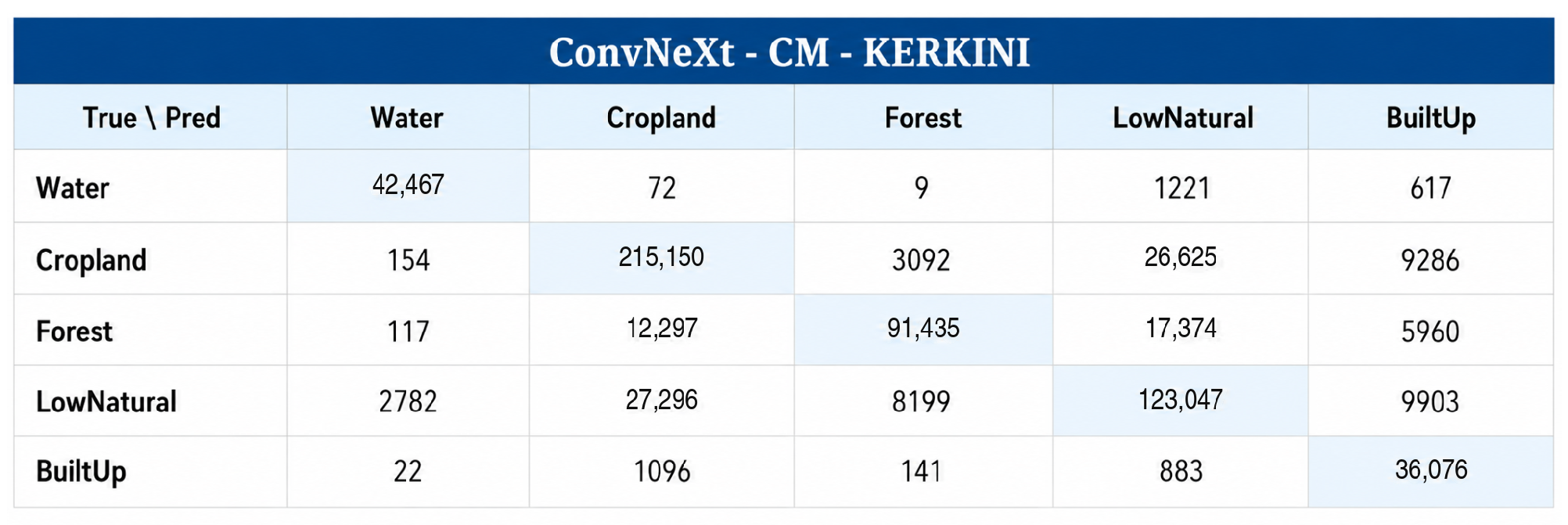
To complement the aggregate performance metrics and provide deeper insights into the classification error distribution, class-wise confusion matrices were generated for the spatial cross-validation in the Lake Kerkini region. Figure 7, Figure 8, Figure 9 and Figure 10 illustrate the class-wise confusion matrices for the CNN, UNet++, ViT and ConvNeXt architectures, respectively.

The error structure reveals that misclassifications are predominantly concentrated among the vegetation-related classes, specifically Cropland, Forest and Low/Natural Vegetation. For instance, examining the UNet++ predictions, 12.0% of reference Cropland pixels are classified as Low/Natural Vegetation, while 11.7% of reference Low/Natural Vegetation pixels are misclassified as Cropland. Furthermore, 14.4% of reference Forest pixels are confused with Low/Natural Vegetation. The traditional CNN architecture exhibits a similar vegetation-related error pathway, with 10.0% of reference Cropland pixels classified as Low/Natural Vegetation, 11.7% of reference Low/Natural Vegetation pixels misclassified as Cropland and 9.4% of reference Forest pixels confused with Low/Natural Vegetation, suggesting that these patterns are data-driven rather than architecture-specific.

These misclassifications reflect the inherent ecological complexity and the overlapping phenological signatures of these broad land cover categories. The Low/Natural Vegetation class acts as a transitional category encompassing shrubland, grassland and herbaceous vegetation, which often shares spectral similarities with both cultivated areas and forested regions throughout the year. In contrast, Water showed consistently high class-specific reliability, while Built-up pixels often achieved high producer-side detection but required more cautious interpretation because of commission errors. Ultimately, this class-wise analysis clarifies that the moderate overall accuracy is largely driven by the semantic and spectral overlap among the aggregated vegetation classes, rather than fundamental limitations in the models’ spatial feature extraction capabilities.

The ViT architecture was also examined to better understand the error structure of the weakest-performing model. In the Lake Kerkini test area, ViT achieved an overall accuracy of 0.7042 and a Kappa coefficient of 0.5983, which are clearly lower than the corresponding CNN and UNet++ results. The main weakness of the ViT model is concentrated in the vegetation-related classes. In particular, only 51.5% of reference Forest pixels are correctly classified, while 20.9% are classified as Low/Natural Vegetation, 14.7% as Cropland and 12.8% as Built-up. This indicates that ViT struggles to distinguish dense vegetation from transitional vegetation and agricultural surfaces in the Lake Kerkini test area.

A second important limitation concerns the Built-up class. Although ViT correctly identifies 94.0% of reference Built-up pixels, the User’s Accuracy of the Built-up class is only 36.9%. Therefore, the high diagonal value for Built-up should not be interpreted as fully reliable Built-up mapping. Instead, it shows that ViT detects most existing Built-up pixels but also assigns many non-Built-up pixels to the Built-up class. Specifically, 61,573 non-Built-up pixels are falsely predicted as Built-up, mainly originating from Cropland Forest and Low/Natural Vegetation. This confirms that the weaker performance of ViT is related not only to omission errors in vegetation classes but also to substantial Built-up commission errors.

The ConvNeXt architecture follows a more balanced error structure than ViT and shows stronger class separation in the Lake Kerkini test area. Based on the ConvNeXt confusion matrix, the model achieves an overall accuracy of 0.7999 and a Kappa coefficient of 0.7235. The class-specific results indicate high correct classification rates for Water and Built-up, with 95.7% of reference Water pixels and 94.4% of reference Built-up pixels correctly classified. However, the main remaining errors again concern the vegetation-related classes. In particular, 10.5% of reference Cropland pixels are classified as Low/Natural Vegetation, 13.7% of reference Forest pixels are classified as Low/Natural Vegetation and 15.9% of reference Low/Natural Vegetation pixels are classified as Cropland. This confirms that ConvNeXt reduces, but does not eliminate, the dominant vegetation-related confusion pathway observed across the other architectures.

Despite the high Producer’s Accuracy of the Built-up class in ConvNeXt, its User’s Accuracy is 58.3%, indicating that Built-up commission errors remain present. Specifically, 25,766 non-Built-up pixels are falsely assigned to the Built-up class, mainly originating from Low/Natural Vegetation, Cropland and Forest. Nevertheless, this behavior is less severe than in the ViT model, suggesting that ConvNeXt provides a more reliable balance between omission and commission errors in the Lake Kerkini test area.

3.3. Class-Wise Confusion Structure in the Lake Doirani Transfer Area

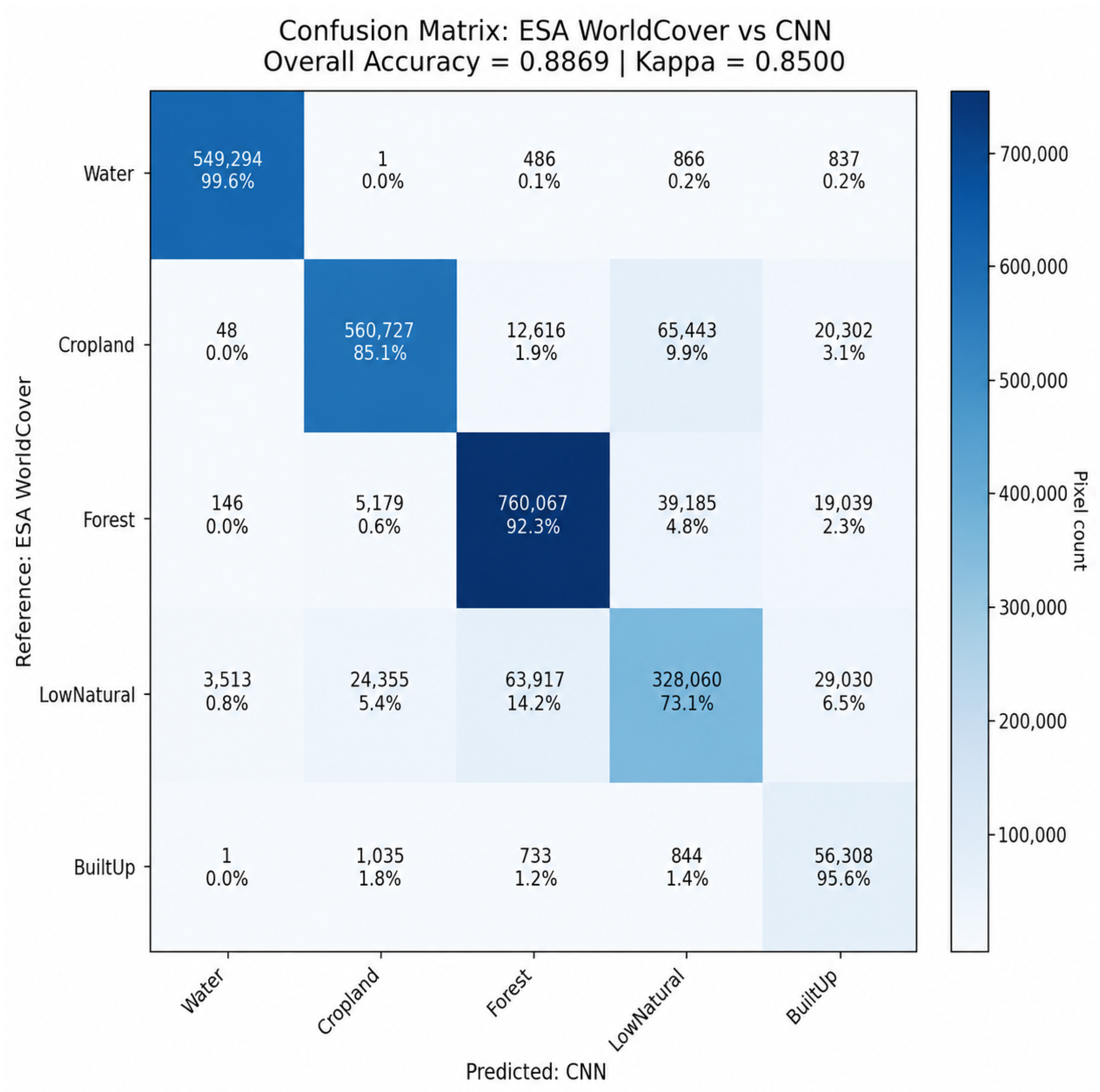
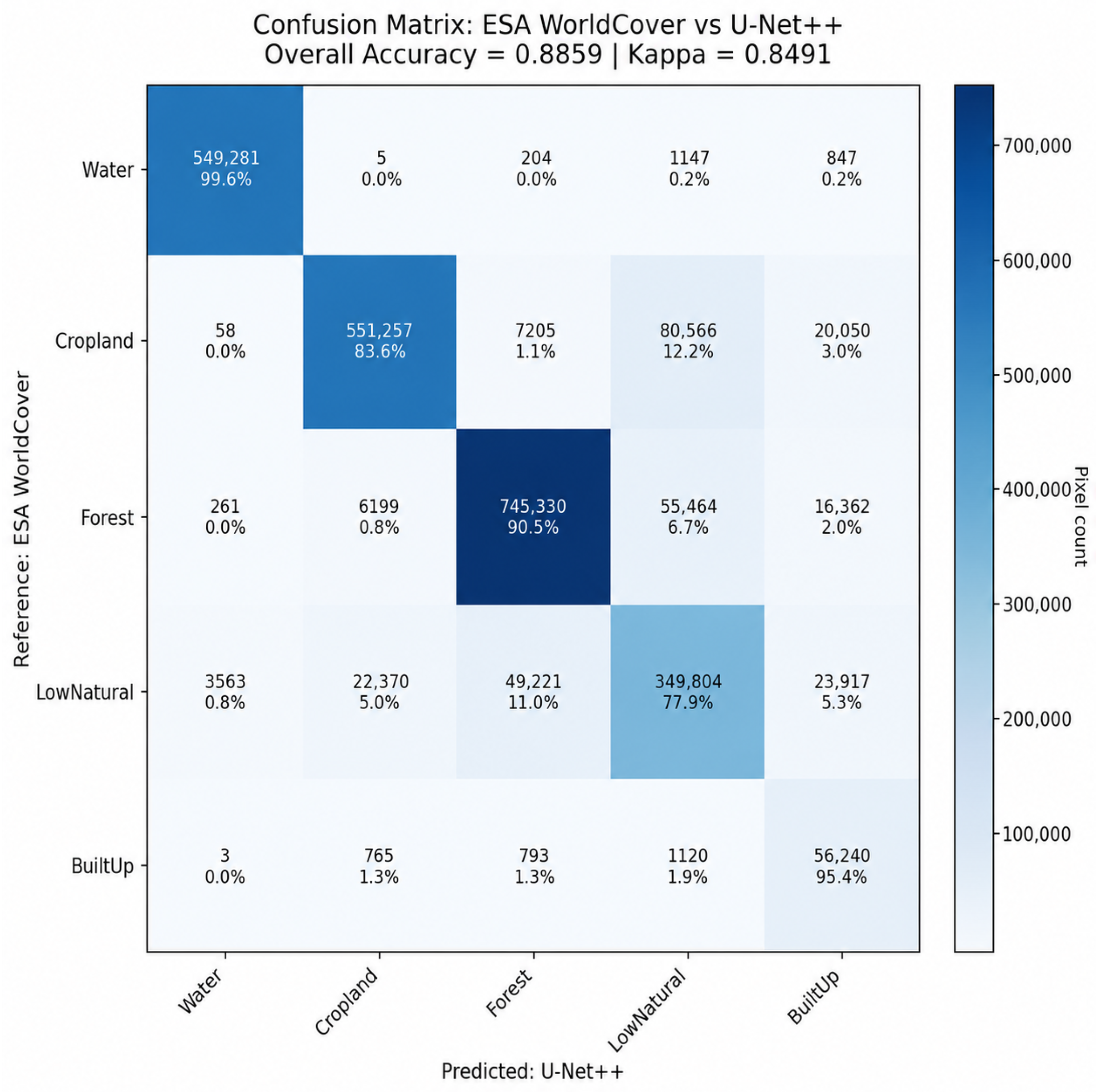
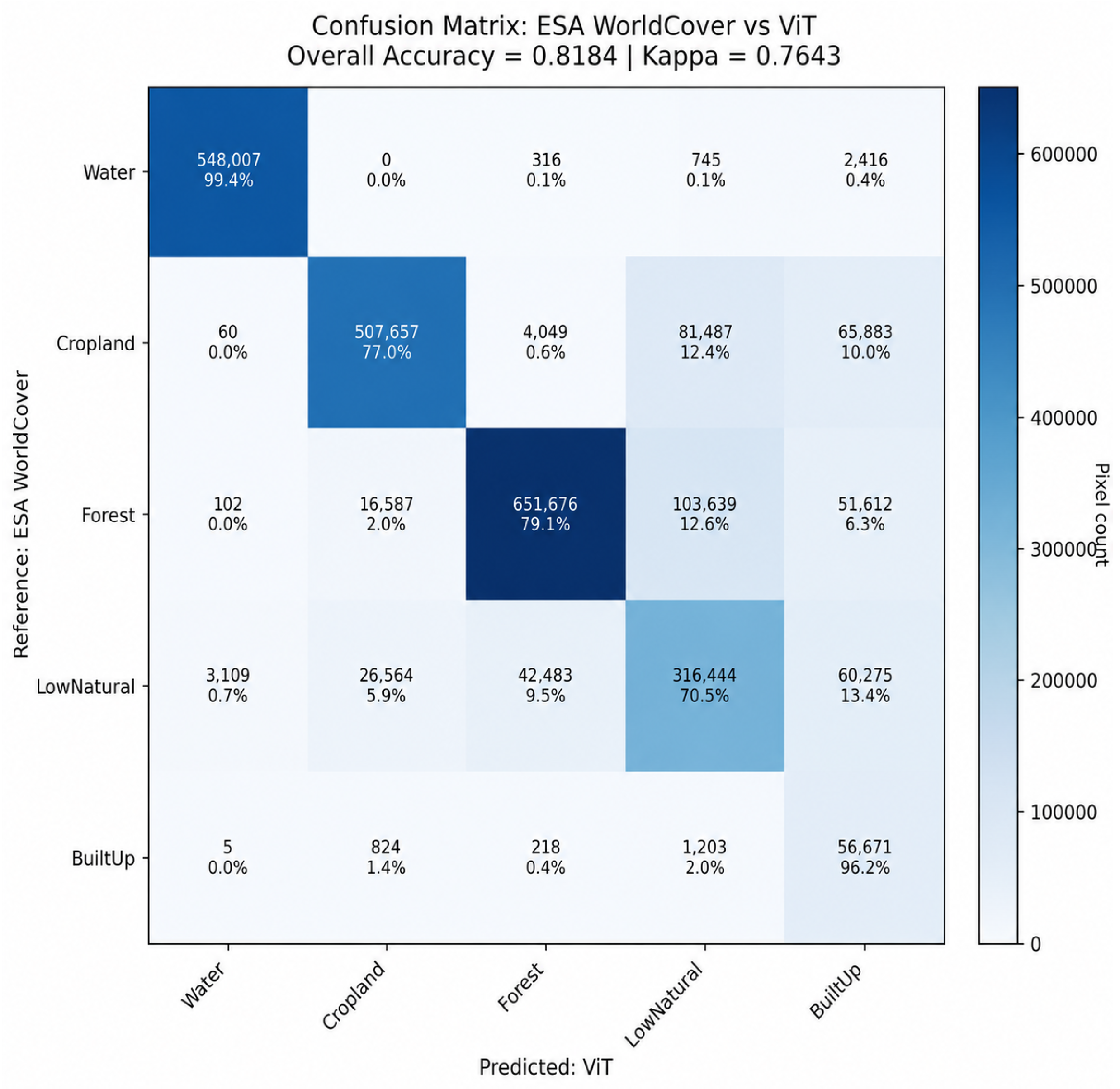
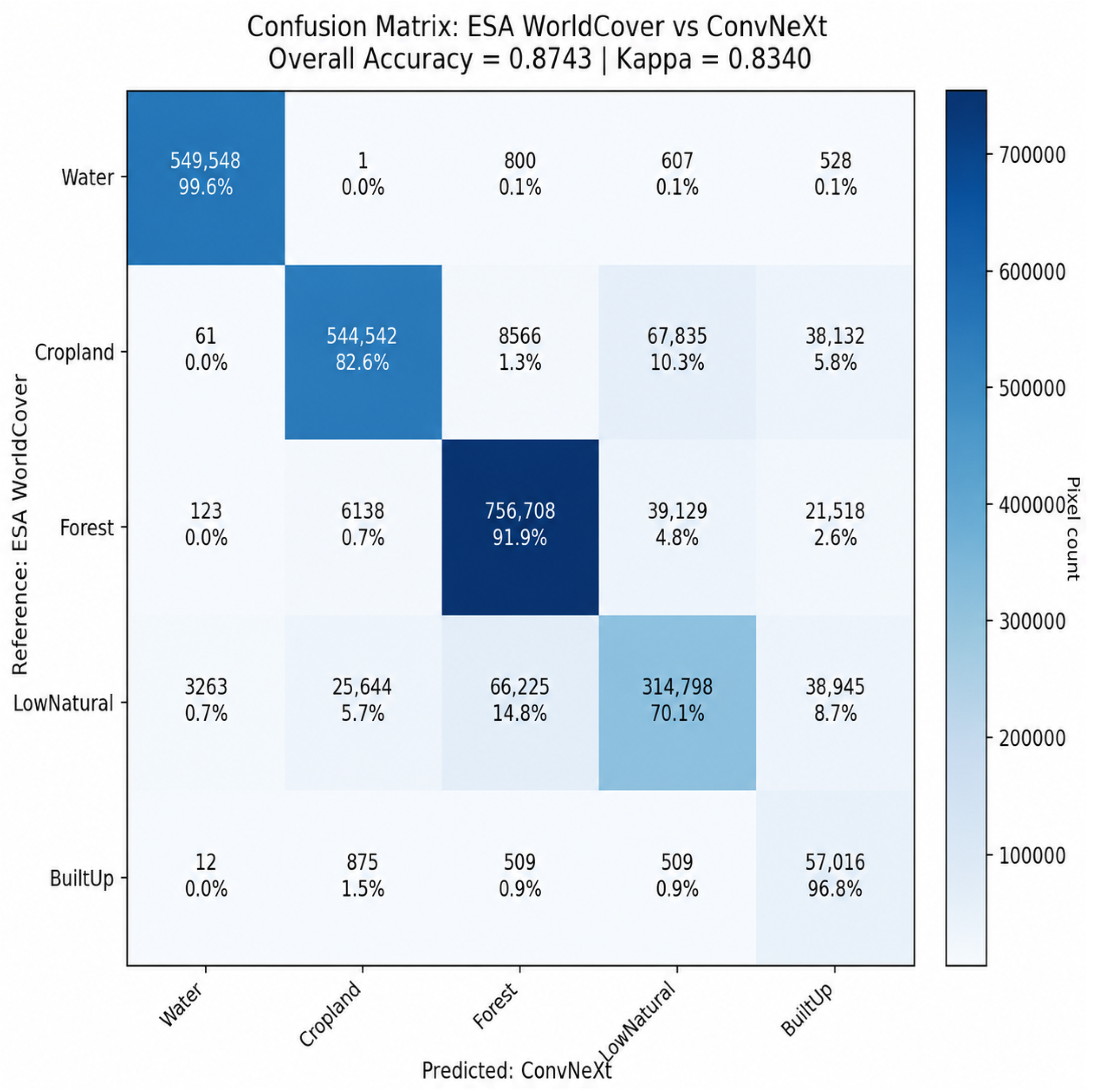
To further evaluate the regional transferability of the trained models, class-wise confusion matrices were generated for the Lake Doirani transfer area using ESA WorldCover as reference data. Figure 11, Figure 12, Figure 13 and Figure 14 present the confusion matrices for the CNN, UNet++, ViT and ConvNeXt architectures, respectively. This analysis allows the transfer performance to be examined beyond aggregate accuracy metrics by identifying the dominant class-specific error pathways.

The results show that CNN and UNet++ achieve the strongest transfer performance in the Lake Doirani area. CNN obtains the highest overall accuracy, with an Overall Accuracy of 0.8869 and a Kappa coefficient of 0.8500, while UNet++ follows very closely with an Overall Accuracy of 0.8859 and a Kappa coefficient of 0.8491. ConvNeXt achieves a slightly lower but still competitive performance, with an Overall Accuracy of 0.8743 and a Kappa coefficient of 0.8340. In contrast, ViT presents the weakest transfer performance, with an Overall Accuracy of 0.8184 and a Kappa coefficient of 0.7643. Therefore, ConvNeXt does not outperform the CNN-based architectures in this transfer experiment, but it provides a clearly more reliable classification structure than ViT.

Across all models, Water is the most stable class. CNN, UNet++ and ConvNeXt correctly classify 99.6% of reference Water pixels, while ViT correctly classifies 99.4%. This indicates that spectrally distinct classes transfer well between areas. The main errors are concentrated in the vegetation-related classes, where agricultural land, forested areas and low or natural vegetation present stronger spectral and semantic overlap.

For ConvNeXt, the Producer’s Accuracy is very high for Water, Forest and Built-up pixels. Specifically, 99.6% of reference Water pixels, 91.9% of reference Forest pixels and 96.8% of reference Built-up pixels are correctly classified. However, the main confusion remains concentrated in the vegetation-related classes. In particular, 10.3% of reference Cropland pixels are classified as Low/Natural Vegetation, while 14.8% of reference Low/Natural Vegetation pixels are classified as Forest. This confirms that, even in the transfer area, the dominant errors are mainly associated with the separation of agricultural land, forest and transitional natural vegetation.

A further issue concerns the reliability of the Built-up class (

Table 8. Built-up class reliability in the Lake Doirani transfer area. Producer’s Accuracy indicates how many reference Built-up pixels were correctly detected, while User’s Accuracy indicates how reliable the pixels predicted as Built-up are.

Model	Overall Accuracy	Kappa	Built-Up PA	Built-Up UA
CNN	0.8869	0.8500	95.6%	44.9%
UNet++	0.8859	0.8491	95.4%	47.9%
ViT	0.8184	0.7643	96.2%	23.9%
ConvNeXt	0.8743	0.8340	96.8%	36.5%

). Although all models detect most reference Built-up pixels, the User’s Accuracy of the Built-up class remains considerably lower than its Producer’s Accuracy. For ConvNeXt, the Built-up Producer’s Accuracy reaches 96.8%, but the Built-up User’s Accuracy is only 36.5%. This means that ConvNeXt successfully detects most existing Built-up pixels, but it also assigns a substantial number of non-Built-up pixels to the Built-up class. Specifically, 99,123 non-Built-up pixels are falsely predicted as Built-up, mainly originating from Cropland, Forest and Low/Natural Vegetation (

Table 9. False Built-up predictions in the Lake Doirani transfer area. Values represent non-Built-up ESA WorldCover pixels that were incorrectly assigned to the Built-up class.

Model	Water	Cropland	Forest	Low/Natural	Total False Built-Up
CNN	837	20,302	19,039	29,030	69,208
UNet++	847	20,050	16,362	23,917	61,176
ViT	2416	65,883	51,612	60,275	180,186
ConvNeXt	528	38,132	21,518	38,945	99,123

). This commission error is substantially lower than that of ViT, which produces 180,186 false Built-up predictions, but it remains higher than the corresponding errors of CNN and UNet++.

Overall, the Lake Doirani transfer results show that CNN and UNet++ provide the most accurate and reliable transfer performance, with nearly identical overall agreement. ConvNeXt remains competitive and improves substantially over ViT, especially in terms of overall accuracy, Kappa agreement and reduced Built-up commission errors. However, ConvNeXt still produces more false Built-up predictions than CNN and UNet++ and it does not resolve the confusion between vegetation-related classes. The main limitation across all architectures is therefore not the detection of spectrally distinct classes such as Water, but the separation of mixed or transitional land-cover categories and the over-assignment of heterogeneous rural pixels to the Built-up class.

3.4. Statistical Evaluation

To assess whether the observed performance differences among the four architectures were systematic across the spatial cross-validation folds, a non-parametric repeated-measures statistical procedure was applied. This choice was motivated by the structure of the experimental design. All architectures were evaluated on the same four held-out spatial folds; therefore, the resulting performance estimates are paired by fold rather than independent observations. Moreover, per-class F1 scores obtained from the same confusion matrix are not independent, because class-wise errors are coupled and class difficulty can act as a strong blocking factor. Consequently, the statistical analysis was performed on the fold-level Macro-F1 scores, using the spatial fold as the blocking factor and the model architecture as the repeated factor.

The fold-level Macro-F1 scores used for the statistical analysis are reported in

Table 10. Fold-level Macro-F1 scores used for the non-parametric repeated-measures statistical analysis. Each row corresponds to one held-out spatial cross-validation fold.

Spatial Fold	CNN	UNet++	ConvNeXt	ViT
Fold 1	0.844807	0.826009	0.816090	0.763357
Fold 2	0.759889	0.771458	0.738847	0.628753
Fold 3	0.795969	0.793538	0.795516	0.657023
Fold 4	0.802793	0.795128	0.799753	0.622602

. Each value represents one aggregate performance estimate for a given architecture on one held-out spatial test fold.

A Friedman test was used to evaluate the null hypothesis that all four architectures have equivalent performance ranks across the four spatial folds. The test indicated a statistically significant overall difference among the architectures (${\chi }_F^2=9.300$, $p=0.0256$). Kendall’s coefficient of concordance was $W=0.775$, indicating strong agreement in the fold-wise ranking pattern.

The mean Macro-F1, standard deviation and average Friedman ranks are reported in

Table 11. Mean fold-level Macro-F1, standard deviation and average Friedman rank for each architecture. Lower average rank indicates better performance.

Architecture	Mean Macro-F1	SD	Average Rank
CNN	0.800864	0.034821	1.25
UNet++	0.796533	0.022424	2.25
ConvNeXt	0.787551	0.033659	2.50
ViT	0.667934	0.065357	4.00

. Lower average rank values indicate better relative performance. CNN obtained the best average rank, followed by UNet++ and ConvNeXt, whereas the tested no-pretraining ViT configuration obtained the weakest average rank.

Post-hoc pairwise comparisons were performed using the Nemenyi procedure on the Friedman ranks. The only pairwise comparison that reached the $\alpha =0.05$ significance level was CNN versus ViT ($p=0.0138$). The remaining comparisons did not reach statistical significance: CNN versus UNet++ ($p=0.6923$), CNN versus ConvNeXt ($p=0.5187$), UNet++ versus ConvNeXt ($p=0.9928$), UNet++ versus ViT ($p=0.2208$) and ConvNeXt versus ViT ($p=0.3543$). Because the analysis is based on only four spatial folds, these pairwise post-hoc results should be interpreted cautiously and should not be over-generalized beyond the present experimental setting.

Overall, the statistical analysis supports a conservative interpretation of the model comparison. The three convolutional architectures, namely CNN, UNet++ and ConvNeXt, showed broadly comparable spatial cross-validation performance, with small differences in mean Macro-F1 and no statistically significant pairwise separation among them. In contrast, the tested no-pretraining ViT configuration ranked last in all four spatial folds and showed the lowest mean Macro-F1 (Figure 15), indicating weaker and less stable performance within the present Sentinel-2 case-study setup. This result should be interpreted as evidence about the specific ViT configuration trained from scratch under the current data regime, rather than as a general conclusion that Vision Transformers are unsuitable for remote-sensing land-cover classification.

3.5. Regional Transferability to Lake Doirani

To evaluate regional transferability, each architecture was applied directly to the independent Lake Doirani test basin without any fine-tuning or domain adaptation. The resulting OA and Macro-F1 scores on the Doirani dataset are reported in

Table 12. Regional transferability performance on the independent Lake Doirani region. Models were deployed directly after training on Lake Kerkini, without fine-tuning.

Architecture	OA	Macro-F1
CNN	0.887	0.832
UNet++	0.886	0.837
ConvNeXt	0.874	0.808
ViT	0.818	0.747

.

The Lake Doirani regional transferability evaluation shows that the CNN and UNet++ architectures achieved the strongest regional transferability among the tested models. CNN obtained the highest OA score, while UNet++ achieved the highest Macro-F1 score, indicating that both architectures generalized well to the independent basin under the present experimental setting. This suggests that convolutional inductive biases and, in the case of UNet++, multi-scale feature aggregation supported stable regional transfer performance from Lake Kerkini to Lake Doirani.

The ConvNeXt model also maintained competitive transferability, although its performance was slightly lower than that of CNN and UNet++. This result indicates that its convolution-based design and Transformer-inspired architectural choices provided reasonable generalization but did not surpass the simpler CNN or the encoder–decoder UNet++ configuration in this regional transferability evaluation.

The ViT configuration produced the lowest transferability scores among the four models, with both OA and Macro-F1 clearly below the convolution-based architectures. This finding suggests that, in the present no-pretraining and limited-domain training setting, the tested Transformer-based model was less robust to regional distribution shifts. Therefore, its performance should be interpreted within this experimental context, as ViT-based approaches may benefit from larger and more geographically diverse training datasets or external pretraining.

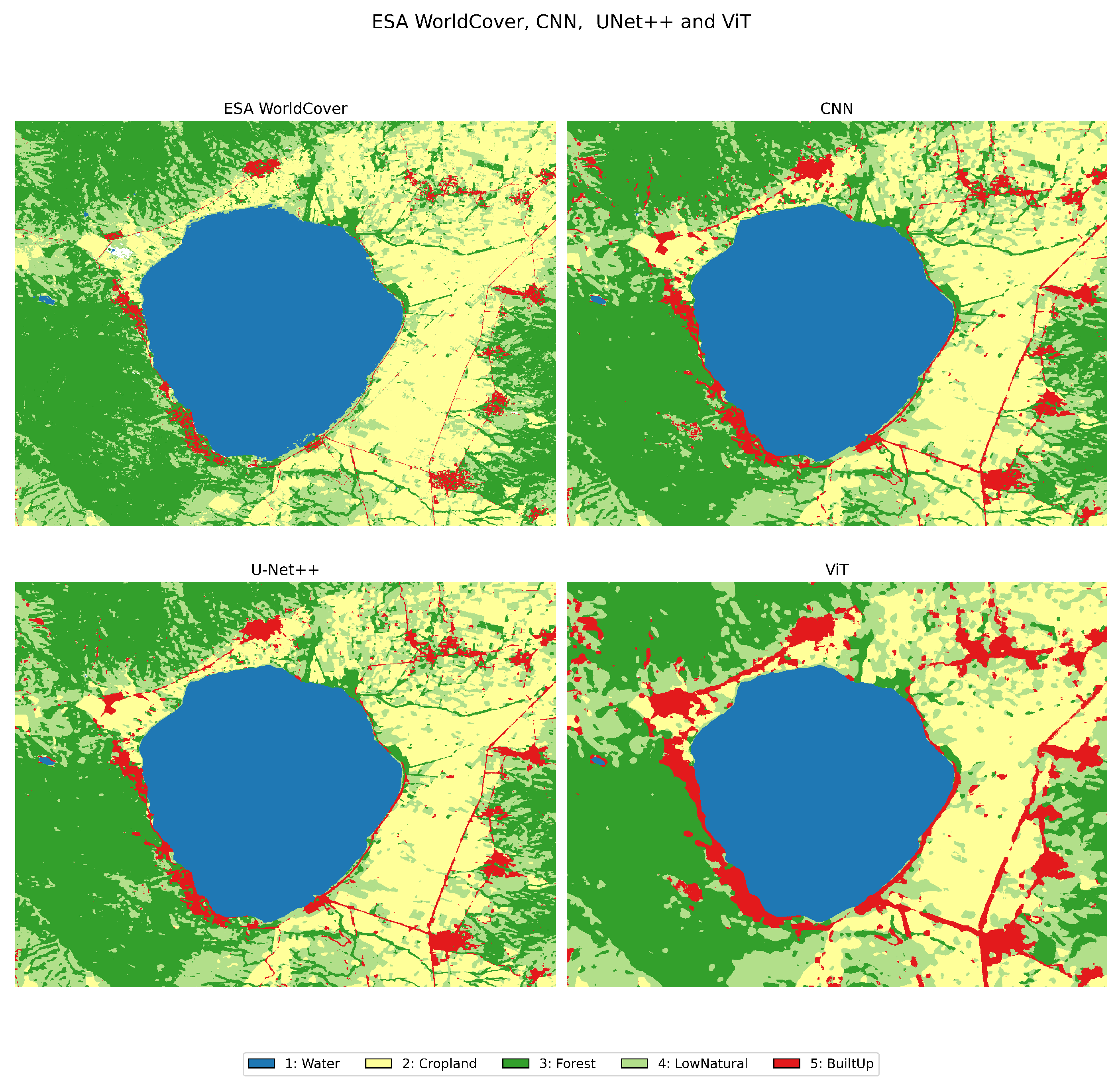
For the visual comparison in Figure 16, a representative subset of outputs is shown to reduce figure size and avoid redundancy. The figure includes the ESA WorldCover reference map, the two strongest-performing models in the transfer experiment, namely CNN and UNet++ and the weakest-performing model, ViT, as a lower-bound comparison. ConvNeXt is therefore excluded from the visual comparison figure, because its performance is already reported quantitatively in Table 12 and it did not represent either the best-performing or the worst-performing transfer case.

Visual inspection of Figure 16 shows that the main spatial differences among the models occur in the terrestrial classes rather than in the mapped water extent. CNN and UNet++ preserve more of the fine-grained Cropland and Low/Natural Vegetation mosaic visible in the WorldCover-derived reference, although some disagreements remain at the transitions among Cropland, Forest and Low/Natural Vegetation and along parts of the lake margin. In contrast, the ViT output is spatially more generalized, with larger homogeneous patches and a visibly stronger overprediction of Built-up areas, particularly along the western and southern shoreline and within the eastern settlement and road network. These spatial patterns are consistent with the confusion-matrix analysis, which identified vegetation-class confusion and Built-up commission errors as important sources of disagreement.

3.6. Band Importance Assessment

To investigate the spectral and seasonal factors driving model predictions, a comprehensive feature importance analysis was performed on an independent external evaluation area following the methodology described in Section 2.7. The consensus importance rankings, derived by averaging the rank positions from the occlusion-based and Gradient × Input attribution methods, are summarized in

Table 13. Top-10 consensus band importance rankings for each architecture, derived by averaging occlusion and Gradient × Input rank positions. Lower rank values indicate higher importance.

CNN		UNet++		ConvNeXt		ViT
Rank	Band	Rank	Band	Rank	Band	Rank	Band
3.5	B12_summer	3.5	B2_summer	3.0	B2_winter	2.0	B2_summer
3.5	B2_winter	4.5	B2_winter	4.0	B2_summer	3.0	B2_winter
4.0	B3_summer	5.5	B12_summer	4.5	B3_summer	5.5	B4_summer
4.5	B2_summer	5.5	B4_winter	5.0	B12_summer	6.5	B3_winter
7.0	B4_summer	6.5	B4_summer	5.0	B4_summer	7.5	B3_summer
7.5	B5_summer	10.5	B2_spring	8.0	B3_winter	9.5	B12_summer
10.0	B12_spring	11.5	B12_autumn	10.5	B4_winter	10.0	B12_autumn
10.5	B12_autumn	12.0	B11_spring	11.5	B2_autumn	10.0	B2_spring
11.0	B4_winter	12.5	B3_summer	13.5	B2_spring	10.5	B5_winter
11.5	B3_winter	13.0	B3_winter	14.0	B4_autumn	12.0	B11_winter

for each architecture.

Several consistent patterns emerge from the consensus rankings across all four architectures. B2 (Blue band) during winter and summer was consistently identified as the most influential input channel, with either the winter or summer acquisition appearing as the top-ranked channel for all architectures. This finding underscores the discriminative value of the Blue spectral region across seasons, capturing the strong phenological contrast between water bodies, bare agricultural fields and evergreen vegetation. The dual high ranking of B2_winter and B2_summer suggests that reduced vegetation activity in winter and drought-induced changes in summer both make surface reflectance differences in the Blue spectrum highly apparent.

The B12 (Short-Wave Infrared, SWIR) band during summer consistently appeared within the top-ranked channels for all four models (rank 3.5–9.5), particularly dominating in the CNN architecture (tied for rank 3.5). The SWIR band is highly responsive to leaf moisture content, canopy water stress and soil moisture, all of which are strongly differentiated during the dry Mediterranean summer. Correspondingly, B3 (Green) and B4 (Red) during summer also ranked prominently across most architectures, reflecting the heightened spectral contrast associated with summer drought stress, senescence and differences between natural and agricultural vegetation classes.

Visible bands from the winter and summer seasons, particularly B3 (Green) and B4 (Red), appeared consistently within the top-10 rankings, highlighting the importance of the key phenological extremes (wet/cold vs dry/hot) for discriminating cropland from forest and low vegetation. The B12 (SWIR) band during autumn and spring was also prominently ranked, especially for the CNN, UNet++ and ViT models, capturing valuable transition-season dynamics.

In contrast, derived spectral indices, including NDVI, NDWI, NDBI and NDRE, were generally ranked outside the top-10 channels and tended to appear in the lower half of the importance spectrum across architectures and seasons. This result should be interpreted cautiously. The indices used in this study are deterministic transformations of raw Sentinel-2 bands that were already included in the same input feature stack. Therefore, their lower attribution scores do not imply that spectral indices are generally uninformative or less useful for land-cover classification. Rather, they suggest that, in the present full-input configuration, these indices may be partly redundant when their constituent reflectance bands are also available to the networks.

This interpretation is particularly relevant for indices such as NDVI and NDWI, which are mathematically derived from combinations of visible, near-infrared and short-wave infrared bands. Under strong feature collinearity, attribution methods such as occlusion and Gradient × Input may distribute importance unevenly between raw bands and derived indices. Consequently, low attribution for an index may simply indicate that similar vegetation-, water-, moisture- or built-up-related information can be recovered by the model from the original spectral channels.

The high degree of agreement in the top-ranked channels across independently trained spatial folds, quantified by Spearman rank correlations, further confirmed the stability of these attributions, indicating that the identified spectral priorities reflect genuine model-learned patterns rather than fold-specific artefacts. Nevertheless, these results should be interpreted as model-specific explanations of the trained networks’ behavior rather than as causal evidence of the standalone physical importance of individual bands or indices. Overall, the feature importance analysis indicates that the Blue (B2), Red (B4) and SWIR (B12) bands during the summer and winter extremes were consistently influential within the present full-feature modeling setup, while derived indices appeared to provide limited additional attribution when the corresponding raw Sentinel-2 bands were already included.

4. Discussion

The results of this case study show that, under spatially separated validation, the three convolution-based architectures formed a clearly stronger and more stable group than the tested no-pretraining Vision Transformer configuration. Numerically, the CNN achieved the highest fold-mean aggregate performance in the Lake Kerkini spatial cross-validation experiment, with an OA of 81.53% and a Macro-F1 of 80.09%. UNet++ followed very closely, with an OA of 80.84% and a Macro-F1 of 79.65%, while also showing the lowest fold-to-fold variability in Macro-F1. ConvNeXt remained competitive, with an OA of 80.09% and a Macro-F1 of 78.76%.

In contrast, ViT produced substantially lower mean performance, with an OA of 70.74% and a Macro-F1 of 66.79%. Therefore, the main architectural conclusion is not that a single convolutional model clearly dominates, but that convolutional architectures were consistently more reliable than the tested no-pretraining ViT configuration in this multi-seasonal Sentinel-2, WorldCover-derived and spatially constrained setting.

This interpretation is supported by the statistical evaluation. Although the CNN was numerically the best model in the fold-mean results, the non-parametric repeated-measures analysis indicated that the small numerical differences among CNN, UNet++ and ConvNeXt were not statistically sufficient to establish a clear ranking among the three convolutional architectures. The Friedman test indicated a significant overall architecture effect across the four spatial folds, while Kendall’s coefficient of concordance showed strong agreement in the fold-wise ranking pattern. In the post-hoc Nemenyi comparisons, the only pairwise difference that reached the 0.05 significance level was between CNN and ViT. Therefore, the statistical evidence should be interpreted conservatively: CNN, UNet++ and ConvNeXt formed a broadly comparable high-performing group, whereas the tested no-pretraining ViT configuration consistently ranked last across the spatial folds, although not all pairwise differences between ViT and the convolutional architectures reached statistical significance under the conservative post-hoc test.

The stronger behavior of the convolutional models is consistent with recent computer-vision evidence showing that convolutional design remains highly competitive, especially when modernized with architectural choices inspired by Transformers. ConvNeXt, for example, was developed by progressively modernizing a ResNet-like convolutional architecture toward Transformer-style design choices, while still retaining a purely convolutional structure [32]. This supports the interpretation that the local spatial priors of convolutional models remain useful for image-classification and segmentation problems. In the present land-cover classification task, such priors are well matched to patch-based Sentinel-2 classification, where many discriminative cues are local or semi-local, including field boundaries, riparian vegetation patterns, forest texture and built-up edges.

UNet++ may additionally benefit from its encoder–decoder structure and nested dense skip pathways. The original UNet++ formulation introduced redesigned skip pathways to reduce the semantic gap between encoder and decoder feature maps [5]. This design is relevant for land-cover classification because the task requires both contextual information and preservation of fine spatial detail, particularly in fragmented agricultural fields, narrow vegetation corridors and mixed land-cover boundaries. However, the present results also show that the additional architectural complexity of UNet++ and ConvNeXt did not produce a statistically significant improvement over the simpler CNN baseline. This is an important point: under the current dataset, input stack and spatial validation design, architectural sophistication alone was not sufficient to establish a clear performance advantage.

The lower performance of the tested ViT configuration should be interpreted carefully. It does not demonstrate that Vision Transformers are generally unsuitable for remote sensing or land-cover classification. Rather, it indicates that the specific ViT configuration evaluated here, trained from scratch without ImageNet, remote-sensing or other external pretraining, was less effective under the available local training-data regime and the strict spatial validation protocol. The original ViT study showed that Vision Transformers can perform very well when pre-trained on large amounts of data and then transferred to smaller recognition benchmarks [33]. Similarly, remote-sensing ViT studies have reported promising scene-classification performance when attention-based models are combined with appropriate training strategies such as transfer learning and data augmentation [34]. Therefore, the present result should be limited to the no-pretraining ViT configuration tested in this study, rather than generalized to all transformer-based remote-sensing models.

The class-wise confusion analysis indicates that most remaining errors were not randomly distributed across classes. In both the Kerkini spatial test folds and the Doirani transfer region, the dominant error pathways involved Cropland, Forest and Low/Natural Vegetation. This pattern is expected given the adopted five-class scheme. The Low/Natural Vegetation class aggregates shrubland, grassland, herbaceous wetland and transitional vegetation, which can overlap spectrally and phenologically with both agricultural fields and sparse or edge forest areas. Previous Sentinel-2 land-cover classification studies have shown that seasonal and spectral–temporal information is important because different land-cover classes exhibit distinct phenological behavior across the year [35]. Similarly, crop-classification studies using multi-temporal Sentinel-2 data emphasize that temporal information helps capture crop phenological stages [36]. Therefore, part of the confusion observed here likely reflects the inherent spectral and phenological overlap among vegetation-related classes, as well as the semantic breadth of the aggregated Low/Natural Vegetation category.

The Built-up class requires particular caution. In Kerkini, some models showed high producer-side detection of reference Built-up pixels, but this did not always translate into equally reliable Built-up predictions. The issue became clearer in the Doirani transfer analysis, where all models detected most reference Built-up pixels but produced low Built-up User’s Accuracy. For example, the Built-up User’s Accuracy ranged from 23.9% for ViT to 47.9% for UNet++, despite producer accuracies above 95% for all architectures. This means that the models tended to over-assign some heterogeneous rural, bare-soil or transitional pixels to the Built-up class. Therefore, the Built-up maps should not be presented as fully reliable urban masks without additional validation or post-processing. This point is important because reporting only OA or producer accuracy would overstate the practical reliability of the Built-up output.

The Lake Doirani experiment provides useful evidence of regional transferability, but its scope should not be overstated. CNN and UNet++ achieved the strongest transfer performance, with CNN obtaining the highest OA and UNet++ the highest Macro-F1. ConvNeXt also transferred reasonably well, while ViT remained the weakest model. However, Doirani is geographically nearby and belongs to a broadly similar Mediterranean context. Moreover, the evaluation was again based on remapped ESA WorldCover-derived reference labels. The results should therefore be interpreted as regional transfer to a nearby independent basin under the same reference-label framework, not as proof of broad geographic generalization. This caution is consistent with the area-of-applicability concept in spatial prediction, according to which model performance estimates are most defensible in areas where the predictor conditions are sufficiently represented by the training data [37].

The feature-importance results suggest that the models relied strongly on specific raw spectral-seasonal channels, especially B2 in winter and summer and B12 in summer. The importance of seasonal information is consistent with Sentinel-2 studies showing that seasonal composites and phenology-based features can improve vegetation and land-cover mapping [35,38]. The prominence of SWIR information is also consistent with prior Sentinel-2 tree-species mapping work, where feature-importance analysis highlighted the relevance of Sentinel-2 SWIR bands [38]. In the present Mediterranean landscape, the high ranking of summer SWIR information is plausible because summer conditions can increase contrast among cropland, natural vegetation, forest and exposed soils. Nevertheless, these results should be treated as model-attribution evidence rather than causal evidence of the standalone physical importance of individual bands.

This caution is especially important for the derived indices. NDVI, NDWI, NDBI and NDRE were generally ranked below the top raw bands, but this does not mean that vegetation, water or built-up indices are generally unimportant for land-cover mapping. The indices are deterministic functions of Sentinel-2 bands that were already included in the same input stack. Under this collinear full-feature setting, the networks may recover equivalent information directly from the raw spectral channels, causing attribution to concentrate on the original bands rather than on the derived indices. More generally, interpretation methods can lead to misleading conclusions if feature dependencies and causal interpretation are not handled carefully [39]. A separate ablation experiment, in which models are retrained with and without spectral indices, would be required to quantify the actual incremental value of these indices.

Finally, the validation design is central to the interpretation of the study. The use of geographically separated test regions and buffer zones reduced spatial leakage and provided a more conservative estimate than random pixel-level splitting. This is important because random cross-validation can produce overly optimistic error estimates when data have spatial, temporal or hierarchical structure, whereas blocked cross-validation is generally more appropriate for estimating performance on new spatial data [10]. At the same time, the labels used in this study were derived from ESA WorldCover 2021 and should be understood as pseudo-reference labels rather than independent field observations. ESA WorldCover 2021 is a 10 m global land-cover product derived from Sentinel-1 and Sentinel-2 data [40]. Independent validation studies of recent 10 m global land-cover products show that accuracy varies across products, classes, regions and heterogeneous landscapes [41]. Consequently, the reported metrics measure agreement with a remote-sensing-derived reference product, not direct field-verified ground-truth accuracy.

Overall, the study shows that multi-seasonal Sentinel-2 imagery combined with spatially rigorous validation can support reliable broad land-cover classification under the spatial and regional conditions examined in this Mediterranean case study. For the present case study, convolution-based models were more reliable than the tested no-pretraining ViT configuration, but the differences among CNN, UNet++ and ConvNeXt were not statistically sufficient to establish a definitive ranking. Future work should validate the framework using independent field or high-resolution reference data, extend testing to multiple years and more distant regions, compare seasonal composites with denser temporal representations and evaluate pretrained transformer or hybrid CNN–Transformer architectures.

5. Conclusions

This study evaluated CNN, UNet++, ConvNeXt and ViT architectures for five-class land-cover classification using multi-seasonal Sentinel-2 composites and WorldCover-derived reference labels. The use of four spatially independent test folds with buffer zones provided a conservative assessment of model behavior under reduced spatial leakage, making the reported results more realistic than those expected from random pixel-level validation.

The main finding is that the convolution-based architectures were more robust than the tested no-pretraining ViT configuration. CNN achieved the highest numerical fold-mean performance in the Lake Kerkini spatial cross-validation experiment (OA = 81.53%, Macro-F1 = 80.09%), followed closely by UNet++ (OA = 80.84%, Macro-F1 = 79.65%) and ConvNeXt (OA = 80.09%, Macro-F1 = 78.76%). The non-parametric repeated-measures statistical evaluation indicated a significant overall architecture effect across the four spatial folds. However, the post-hoc Nemenyi comparisons did not support a statistically significant separation among CNN, UNet++ and ConvNeXt. Therefore, the results do not support a definitive ranking among the three convolutional architectures; they support the broader conclusion that convolutional architectures formed the reliable high-performing model family in this experimental setting. The tested no-pretraining ViT configuration showed clearly lower numerical performance (OA = 70.74%, Macro-F1 = 66.79%) and ranked last across all four spatial folds, although the conservative post-hoc analysis showed a statistically significant pairwise difference only between CNN and ViT.

The external Lake Doirani experiment further showed that CNN and UNet++ transferred best to the nearby independent basin without fine-tuning. CNN achieved the highest OA, while UNet++ achieved the highest Macro-F1. ConvNeXt remained competitive, whereas ViT again produced the weakest transfer performance. This finding supports the regional transfer potential of convolution-based models, but only within the limits of the study design: Doirani is a nearby Mediterranean region and the evaluation used the same WorldCover-derived reference-label framework. The result should not be presented as proof of broad geographic generalization.

The main classification errors were concentrated among Cropland, Forest and the aggregated Low/Natural Vegetation class. This reflects both spectral overlap and the broad semantic definition of the Low/Natural Vegetation category. The Built-up class also requires caution, especially in the transfer region, because high detection of reference Built-up pixels was accompanied by low User’s Accuracy and substantial false Built-up predictions from non-urban classes. These findings show that aggregate accuracy alone is not sufficient for assessing the operational reliability of the maps.

The feature-attribution analysis indicated that the models relied mainly on raw spectral-seasonal channels, particularly Blue-band information in winter and summer and SWIR information in summer. Derived indices such as NDVI, NDWI, NDBI and NDRE received lower attribution scores in the full-feature setting, most likely because their constituent raw Sentinel-2 bands were already available to the networks. This should be interpreted as attribution-level redundancy, not as evidence that spectral indices are generally unimportant.

Overall, the study shows that multi-seasonal Sentinel-2 imagery combined with spatially rigorous validation can support reliable broad land-cover classification under the spatial and regional conditions examined in this Mediterranean case study. For the present case study, convolution-based models were more reliable than the tested no-pretraining ViT configuration. The reported OA and Macro-F1 values quantify agreement with the WorldCover-derived reference labels and should not be interpreted as independently field-validated land-cover accuracy. Future work should validate the framework using independent field observations or systematically visually interpreted high-resolution reference samples, extend testing to more years and more distant regions, compare seasonal composites with denser temporal representations and evaluate pretrained transformer or hybrid CNN–Transformer architectures.