GTSNet: A Global Topography-Aware Segmentation Network for Remote Sensing Identification of Unstable Rock Masses

Highlights

What are the main findings?

• A novel Global Topography-aware Segmentation Network (GTSNet) was developed by integrating UAV imagery and DEM data for unstable rock mass identification.
• GTSNet achieved superior performance on seven hydropower engineering datasets, reaching 90.14% overall accuracy and 60.97% IoU, outperforming six state-of-the-art segmentation models.

What are the implications of the main findings?

• DEM-derived topographic constraints effectively reduce false positives caused by complex terrain, shadows, and visually similar background features.
• The proposed framework provides an efficient and reliable tool for geological hazard investigation and engineering safety assessment in mountainous hydropower regions.

Abstract

The high-precision identification of unstable rock masses in rugged terrain is important for engineering safety and geological hazard prevention. However, shadow occlusion, complex backgrounds, and blurred boundaries caused by rugged terrain often limit the performance of optical feature-based segmentation models, resulting in missed detections and false positives. In this study, to address this issue, we propose a dual-modality deep learning network, named the Global Topography-aware Segmentation Network (GTSNet), that integrates high-resolution unmanned aerial vehicle (UAV) imagery and digital elevation model (DEM) data. The proposed network introduces DEM-derived terrain-semantic information into optical feature modeling through a multi-scale Topography-aware Fusion Module. By using high-level geomorphological context to adaptively recalibrate low-level spatial details, GTSNet improves boundary representation and reduces interference from complex backgrounds. Experiments were conducted on one unstable rock mass dataset compiled from UAV data collected at seven alpine canyon hydropower engineering areas in China. The results show that GTSNet achieved an overall accuracy (Acc) of 90.14%, an F1-score of 75.75%, and an intersection over union (IoU) of 60.97%, showing higher segmentation performance than the six compared semantic segmentation networks under the same RGB + DEM input setting. In addition, GTSNet obtained a Precision of 74.87% and a Recall of 76.66%, indicating a more balanced performance between missed detections and false positives. The results suggest that the integration of RGB imagery and DEM-derived terrain information, together with global context modeling and topography-aware feature fusion, contributes to improved unstable rock mass segmentation in complex canyon environments. This study provides a useful deep learning framework for UAV-based unstable rock mass interpretation in hydropower engineering areas.

1. Introduction

China is one of the countries most vulnerable to geological disasters worldwide. The investigation and identification of collapses, landslides, and surface fractures have long been central topics in geoscience research [1,2]. Unstable rock masses, as the primary source of rockfall hazards in mountainous regions, are characterized by strong suddenness, high destructiveness, and wide impact ranges [3,4]. Once destabilized, they can directly threaten transportation corridors, hydropower infrastructures, and residential areas, posing serious risks to human life, property, and the long-term safety of major engineering projects [5]. Therefore, achieving high-precision identification and real-time monitoring of unstable rock masses is an urgent requirement for improving geological disaster prevention in mountainous areas.

With the development of remote sensing platforms and sensor technologies, high-resolution remote sensing imagery has been widely used in geological disaster identification. Compared to traditional field surveys, remote sensing enables the rapid acquisition of surface information over large areas and effectively improves the efficiency of hazard detection [6,7]. Among these approaches, UAV remote sensing, with its high spatial resolution and operational flexibility, can efficiently acquire detailed surface information in complex and hazardous environments [8,9,10]. It is particularly advantageous in mountainous canyon regions where geological disasters frequently occur, providing robust satellite data for fine-scale identification and investigation [11,12]. Previous studies have shown that integrating UAV aerial imagery with point cloud data, 3D laser scanning, and Building Information Modeling (BIM) technology can achieve centimeter-level 3D reconstruction, providing strong support for the detailed structural analysis of hazard bodies [13]. In addition, UAV-derived products such as digital orthophoto maps (DOMs) and digital surface models (DSMs) can effectively characterize micro-topographic features under complex terrain conditions and have been widely used in landslide mapping, rockfall detection, and slope structure analysis [14,15]. Moreover, combining high-resolution UAV imagery with DEM and machine learning methods can further improve the efficiency of landslide detection [5,16,17].

In recent years, the rapid development of deep learning and computer vision has further driven remote sensing image interpretation toward automation and intelligence, with these methods being widely adopted in geological disaster identification. Compared with traditional machine learning methods, deep learning models integrate multi-layer feature extraction modules to achieve strong feature representation capability, significantly improving the accuracy of disaster monitoring [15,18]. Due to the complex semantic and background characteristics of remote sensing images, convolutional neural networks (CNNs), object detection models (e.g., Faster R-CNN), and semantic segmentation networks (e.g., U-Net) have become research hotspots [19,20,21]. In addition, foundation models (e.g., DeepLabV3+ and MaskFormer) provide new approaches for remote sensing image segmentation and show strong performance in complex background object recognition [22,23,24]. Lie et al. proposed an improved U-Net model for the automatic extraction of post-earthquake landslides from aerial remote sensing imagery [25]; Rukundo et al. systematically investigated the effect of image size on segmentation accuracy [26]; Ge et al. applied deep learning to rock point cloud analysis to achieve fine extraction of structural faults [27]; and Wang et al. applied CNN-based change detection networks to landslide mapping for improved accuracy and feature representation [19]. Through these applications, multi-source remote sensing data fusion has gradually become a mainstream approach. Cheng et al. constructed a dual-branch network to fuse features from spectral imagery and a DEM, which effectively improved the robustness of the recognition method [28]. Menegoni et al. used RPAS-based photogrammetric surveys and DOMs to improve rock slope stability assessment and rockfall volume estimation through multi-source data integration [29]. These studies demonstrated that incorporating topographic information can effectively compensate for the limitations of single optical features and improve the ability to distinguish complex surface objects.

Although these studies have achieved significant progress in typical geological hazard detection, the remote sensing-based identification of unstable rock masses still faces many challenges. Due to the complex terrain conditions of unstable rock masses, which are mainly distributed on steep slopes and canyon cliffs, images are often affected by strong shadow occlusion. At the same time, they usually have a small spatial scale and unclear boundaries, and show limited spectral differences from surrounding bedrock or weathered debris [30,31]. As a result, methods based on single features often fail to achieve reliable performance [32,33]. From the perspective of remote sensing mechanisms, unstable rock masses differ not only in spectral information, but also show certain patterns in texture, shape, and topographic attributes such as elevation [34,35]. Therefore, fusing multi-source features to improve object representation has become a key direction for improving recognition accuracy [36]. Existing studies have shown that combining a DEM with optical imagery can introduce important terrain-related geometric information and improve the description of the spatial structure of hazard bodies [37,38].

On the other hand, existing deep learning methods still have limitations in the detection of unstable rock masses. First, model performance depends heavily on large-scale and high-quality labeled data, while samples of unstable rock masses are difficult to obtain and existing datasets are limited in size [39,40]. Second, most studies focus on large-scale hazards such as landslides, with relatively less attention given to small-scale and highly heterogeneous targets like unstable rock masses [41,42]. In addition, existing methods mostly rely on simple feature stacking and cannot fully exploit the deep complementary information within multi-source data. At the same time, due to differences in terrain type, weathering degree, and rock mass structure, unstable rock masses in different regions show clear inconsistencies in spectral response and spatial distribution [43,44,45,46], limiting the generalization ability of models in cross-region applications. Therefore, it is necessary to select representative typical areas to build training samples and improve the stability and applicability of the method.

Against this background, large-scale water conservancy projects such as hydropower stations, water control hubs, and pumped storage power stations have become important study areas for unstable rock mass detection. These areas are usually located in high-mountain and canyon regions, with steep slopes, fractured rock, and complex geological conditions. They are also strongly affected by engineering activities, which can easily trigger or intensify the instability of unstable rock masses, making them typical zones of concentrated hazards. Once collapse occurs, it not only threatens the safe operation of dams and related facilities, but may also trigger cascading secondary disasters, causing serious impacts on downstream residential areas and energy systems. Therefore, the detailed detection of unstable rock masses in water conservancy project areas is of important engineering safety significance and socio-economic value.

In this study, we use high-resolution UAV imagery from several typical high-mountain canyon water conservancy project areas to construct a dataset for unstable rock mass detection. By designing a new feature extraction module and reconstructing its deep learning architecture, a Global Topography-aware Segmentation Network (GTSNet) is developed that integrates spectral, texture, and topographic features. The network extracts multi-level local features using a convolutional encoder and introduces a Transformer to capture global topographic context. A topography-aware top-down fusion module is used to inject high-level geomorphic semantics into low-level features, enabling multi-scale feature recalibration and boundary enhancement. A progressive decoder is applied to restore spatial resolution, balancing local detail and global semantic interaction, and making the method suitable for steep terrain conditions in water conservancy project areas. Our study achieves the following: (1) a specialized dataset for unstable rock mass detection is built based on high-resolution remote sensing imagery and field validation data; (2) a dual-modal network, GTSNet, is developed by integrating optical imagery and DEM information, jointly modeling appearance features and terrain-related geometric information to achieve the fine-grained segmentation of unstable rock masses; (3) experiments are conducted in typical water conservancy project areas to evaluate accuracy and generalization ability under complex backgrounds, providing decision support for disaster prevention and mitigation in engineering areas.

2. Methodology

2.1. Model Overview

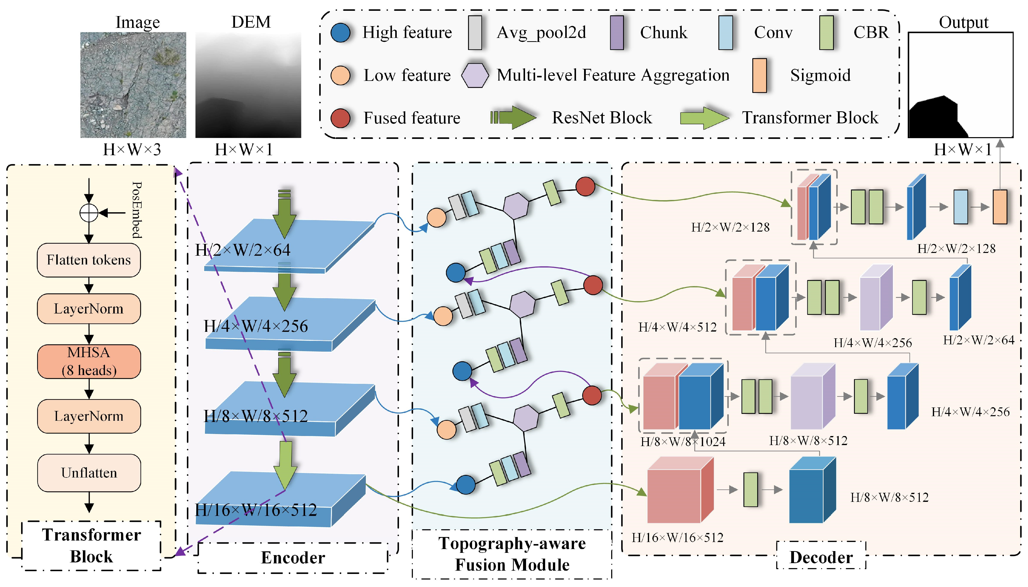
To address the problem of unstable rock mass detection within hydropower station areas under complex mountainous conditions, where local appearance is similar but geomorphic backgrounds are highly heterogeneous, we propose a GTSNet that integrates optical imagery and DEM information (Figure 1).

$$X=\mathit{Cat} (I_{\mathit{rgb}}, D)\in R^{4\times H\times W}$$

(1)

Here $I_{\mathit{rgb}}\in R^{3\times H\times W}$ is the optical image, and $D\in R^{1\times H\times W}$ is the DEM. H and W are the height and width of the input image, respectively.

Overall, GTSNet first uses a convolutional encoder to extract multi-level local texture and semantic features, then introduces a Transformer in the last stage to capture long-range dependencies and global topographic context. Then, a topography-aware top-down fusion module is used to progressively inject high-level geomorphic semantics into low-level high-resolution features, enabling multi-scale feature recalibration and boundary enhancement. Finally, a progressive decoder is used to gradually recover spatial resolution and produce the unstable rock mass segmentation results. This framework balances local detail preservation, global context modeling, and cross-scale semantic interaction, and is well suited for unstable rock mass detection under typical terrain-constrained conditions in hydropower station areas.

2.2. Feature Extraction Module

Unstable rock masses usually have a small spatial scale, fragmented boundaries, and irregular shapes, which means that the encoder must preserve fine details while maintaining strong high-level semantic representation ability. To address this, a hierarchical feature extraction strategy is adopted. The first three stages use a ResNet50 convolutional backbone to extract local structural features and mid-level semantic features, while in the fourth stage, Transformer blocks are introduced after convolutional downsampling to build high-level representations with a global receptive field. If we let the multi-level features produced by the encoder be F₁, F₂, F₃, and F_4, their sizes are as follows:

$$\begin{array}{c}{F}_1\in R^{64 \times {\displaystyle \frac{\mathrm{H}}{2}} \times {\displaystyle \frac{\mathrm{W}}{2}}}\\ F_2\in R^{256 \times {\displaystyle \frac{\mathrm{H}}{4}} \times {\displaystyle \frac{\mathrm{W}}{4}}}\\ F_3\in R^{512 \times {\displaystyle \frac{\mathrm{H}}{8}} \times {\displaystyle \frac{\mathrm{W}}{8}}}\\ F_4\in R^{512 \times {\displaystyle \frac{\mathrm{H}}{16}} \times {\displaystyle \frac{\mathrm{W}}{16}}}\end{array}$$

(2)

Here, F₁, F₂ and F₃ are shallow to mid-high convolutional features, while F₄ is the high-level global feature modeled by the Transformer. This hybrid encoding strategy combines the advantages of convolutional networks in local texture representation with the ability of Transformers in global relationship modeling. The former helps capture local details such as unstable rock mass boundaries, crack shadows, and exposed rock textures, while the latter is more suitable for describing large-scale geomorphic backgrounds such as steep slopes, valley sidewalls, and free-face zones.

When only convolution operators are used, feature responses are mainly constrained by local neighborhoods, while unstable rock mass interpretation often depends on the overall geomorphic environment of the target area. To improve the global context representation ability of the encoder, a Transformer block is introduced in the last stage. First, the output feature from the third stage is downsampled by a convolution operation with stride 2. Then, to alleviate the lack of spatial position information in pure attention modeling, a depthwise separable convolution-based positional encoding is introduced before the self-attention calculation:

$${\tilde{F}}_4 = F_3^{\downarrow } + \mathit{PEG}(F_3^{\downarrow })$$

(3)

Here, $\mathit{PEG}(·)$ is the positional encoding generation operator. The two-dimensional feature map is then flattened into a sequence, followed by multi-head self-attention and a feed-forward network:

$$Z_1 = Z_0 + \mathrm{MHSA}\left(\mathrm{LN}\right({\mathrm{Z}}_0\left)\right)$$

(4)

$$Z_2=Z_1+\mathrm{MLP}\left(\mathrm{LN}\right(Z_1\left)\right)$$

(5)

Here, ${Z_0 = \mathrm{Flatten}(\stackrel{\mathrm{~}}{\mathrm{F}}}_4)$ and $\mathrm{LN}(·)$ is layer normalization. Finally, the sequence is reshaped back into a two-dimensional space to obtain the high-level global feature F₄.

It should be noted that the Transformer is only applied in the last stage. This is because shallow features mainly focus on fine-grained details such as boundaries and textures, and convolutional structures are sufficient for local representation at this level. In contrast, the highest-level features have a stronger semantic abstraction ability. Introducing global attention at this stage enables the modeling of cross-region topographic relationships with a manageable computational cost, while providing stable global semantic priors for subsequent multi-scale fusion. Therefore, this design reduces model complexity while improving the encoder’s ability to capture overall geomorphic structure and provides a global receptive field for the subsequent fusion modules.

Table 1. Information of the feature extraction network module.

Stage	Input Feature Size	Encoder Module	Number of Output Channels	Output Size
1	$4 \times \mathrm{H} \times \mathrm{W}$	ResNet50 shallow convolutional encoding	64	${\displaystyle \frac{\mathrm{H}}{2}} \times {\displaystyle \frac{\mathrm{W}}{2}}$
2	$64 \times {\displaystyle \frac{\mathrm{H}}{2}} \times {\displaystyle \frac{\mathrm{W}}{2}}$	ResNet50 mid-level convolutional encoding	256	${\displaystyle \frac{\mathrm{H}}{4}} \times {\displaystyle \frac{\mathrm{W}}{4}}$
3	$256 \times {\displaystyle \frac{\mathrm{H}}{4}} \times {\displaystyle \frac{\mathrm{W}}{4}}$	ResNet50 deep convolutional encoding	512	${\displaystyle \frac{\mathrm{H}}{8}} \times {\displaystyle \frac{\mathrm{W}}{8}}$
4	$512 \times {\displaystyle \frac{\mathrm{H}}{8}} \times {\displaystyle \frac{\mathrm{W}}{8}}$	$3 \times 3$ stride convolution + Transformer block	512	${\displaystyle \frac{\mathrm{H}}{16}} \times {\displaystyle \frac{\mathrm{W}}{16}}$

shows the detailed configuration of the feature extraction module. It can be seen that the first three stages use a convolutional backbone to progressively extract local features and mid-level semantic features, while the fourth stage uses “convolutional downsampling + Transformer” to form global semantic representations for the subsequent topography-aware fusion.

2.3. Topography-Aware Fusion Module (TFM)

A key challenge in unstable rock mass detection is that similar local textures may correspond to completely different semantic categories under different topographic backgrounds. For example, similar exposed rock textures may appear in unstable rock mass areas on steep slopes, but may also correspond to ordinary exposed rock surfaces. If detection relies only on shallow texture responses, false detections are likely to occur. In contrast, relying only on high-level semantic responses may weaken boundary and detail information. To address this problem, a Topography-aware Fusion Module is designed to progressively use large-scale geomorphic semantics from high-level features to modulate low-level high-resolution features, thereby incorporating terrain-related geometric cues while preserving boundary details.

In contrast to conventional Feature Pyramid Networks or simple concatenation strategies, this model does not directly perform linear fusion of multi-scale features. Instead, a Multi-scale Topography-Aware Module is used to apply pixel-wise modulation to low-level features. The core idea is to treat the topographic context and the global semantics encoded in high-level features as conditional priors to adjust the response strength of different spatial locations in low-level features. Meanwhile, considering that unstable rock mass boundaries usually correspond to local elevation changes or slope discontinuities in the DEM, the module further enhances the high-frequency components in low-level features to highlight potential boundary information. Therefore, the module does not perform a simple multi-scale aggregation, but rather a local feature recalibration process guided by large-scale geomorphic semantics.

Let the high-level input feature be $\mathrm{H} \in {\mathrm{R}}^{{\mathrm{C}}_{\mathrm{h}}\times \mathrm{h}\times \mathrm{w}}$, and the low-level input feature be $\mathrm{L} \in {\mathrm{R}}^{512\times {\displaystyle \frac{\mathrm{H}}{8}}\times {\displaystyle \frac{\mathrm{W}}{8}}}$. First, bilinear interpolation is applied to the high-level feature to align its spatial resolution with the low-level feature:

$$H^{\uparrow } = \mathrm{UP}(H)$$

(6)

Then, the upsampled high-level feature is used to generate the scaling and shifting parameters:

$$\left[\gamma ,\beta \right] = \varphi \left(H^{\uparrow }\right)$$

(7)

where $\varphi (·)$ denotes a convolutional mapping function. The scaling parameter is normalized using a sigmoid function:

$$\gamma = \mathsf{\sigma }\left(\mathsf{\gamma }\right)$$

(8)

To enhance local boundary-related variations in the low-level feature, a local average response is first computed through average pooling:

$$L_{avg} = \mathrm{AvgPool}\left(L\right)$$

(9)

The locally varying high-frequency component is then obtained as follows:

$$E=L-L_{avg}$$

(10)

Here, $L_{\mathit{avg}}$ is the local average response, and E is the locally varying high-frequency component. In unstable rock mass scenes, such high-frequency information usually corresponds to cliff edges, slope break lines, and abrupt elevation changes. Then, a depthwise convolution is applied to further extract edge-enhanced information, yielding the refined low-level feature:

$$\widetilde{L }= L + {\mathrm{DWConv}}_{3\times 3}(E)$$

(11)

On this basis, the pixel-wise parameters generated from high-level semantics are used to perform spatially variant modulation on the enhanced low-level feature:

$$\widehat{L }= \gamma \odot \tilde{L}+\beta$$

(12)

Here, $\tilde{L}$ represents the low-level features after edge enhancement, $\widehat{L}$ is the low-level feature after spatially variant modulation, and $\odot$ represents element-wise multiplication. In contrast to channel attention with uniform weights, this design assigns different modulation strengths to different spatial locations, making it more suitable for mountainous scenes with highly heterogeneous terrain distribution.

Finally, the modulated low-level feature is concatenated with the upsampled high-level feature, and a convolution operation is applied to obtain the output of the current stage:

$$F_{\mathrm{out}} = \psi \left(\mathrm{Cat}\right(\widehat{L},H^{\uparrow }\left)\right)$$

(13)

Here, $\psi (·)$ is the convolutional fusion function, and $F_{\mathrm{out}}$ is the fused feature at the current stage. Through this process, high-level macroscopic topographic information and low-level local details are effectively complemented within a unified framework.

In the network implementation, this module is performed in a top-down manner with a three-level cascade. Let the encoder outputs be F₁, F₂, F₃, and F₄, the fusion process can be expressed as follows:

$$F_3^{\prime } = M(F_4,F_3)$$

(14)

$$F_2^{\prime }=M(F_3^{\prime },F_2)$$

(15)

$$F_1^{\prime }=M(F_2^{\prime },F_1)$$

(16)

Here, $M(·)$ is the Multi-scale Topography-Aware Module. Finally, the fused multi-scale feature set is obtained as $\left\{F_1^{\prime },F_2^{\prime },F_3^{\prime },F_4^{\prime }\right\}$.

This cascaded design has three main advantages. First, the global topographic priors carried by high-level Transformer features are progressively propagated to shallow layers, so that high-resolution features are no longer dependent only on local appearance but are also constrained by macroscopic geomorphic semantics. Second, the edge enhancement branch explicitly preserves local high-frequency information, which helps improve boundary completeness and localization accuracy of unstable rock masses. Finally, pixel-wise modulation has stronger spatial adaptability than simple concatenation or summation and can better represent the spatial heterogeneity of unstable rock masses in different geomorphic positions such as ridge tops, cliff faces, and valley sidewalls. From an application perspective, this module essentially builds a recognition mechanism that constrains local discrimination with macroscopic geomorphology, which can effectively reduce misclassification caused by confusing objects such as exposed rock, shadows, and artificial cut slopes. Detailed information on TFM is provided in Algorithm 1.

Algorithm 1. Topography-aware Fusion Module (TFM).

Input: XL ∈ ${\mathrm{R}}^{\mathrm{B}\times {\mathrm{C}}_{\mathrm{l}}\times {\mathrm{H}}_{\mathrm{l}}\times {\mathrm{W}}_{\mathrm{l}}}$   //Low-level features XH ∈ ${\mathrm{R}}^{\mathrm{B}\times {\mathrm{C}}_{\mathrm{H}}\times {\mathrm{H}}_{\mathrm{H}}\times {\mathrm{W}}_{\mathrm{H}}}$ //High-level features Output: Y ∈ ${\mathrm{R}}^{\mathrm{B}\times {\mathrm{C}}_{\mathrm{l}}\times {\mathrm{H}}_{\mathrm{l}}\times {\mathrm{W}}_{\mathrm{l}}}$  1. // Step 1: Low-level high-frequency enhancement  2. ${\mathrm{X}}_{\mathrm{a}\mathrm{v}\mathrm{g}}\leftarrow \mathrm{A}\mathrm{v}\mathrm{g}\mathrm{P}\mathrm{o}\mathrm{o}\mathrm{l}2\mathrm{d}\left({\mathrm{X}}_{\mathrm{L}}\right)$  3. ${\mathrm{X}}_{\mathrm{e}\mathrm{d}\mathrm{g}\mathrm{e}}\leftarrow {\mathrm{X}}_{\mathrm{L}}-{\mathrm{X}}_{\mathrm{a}\mathrm{v}\mathrm{g}}$  4. ${\mathrm{X}}_{\mathrm{L}\mathrm{E}}\leftarrow {\mathrm{C}\mathrm{o}\mathrm{n}\mathrm{v}(\mathrm{X}}_{\mathrm{e}\mathrm{d}\mathrm{g}\mathrm{e}}$)  5. // Step 2: High-level feature up-sampling  6. ${\mathrm{X}}_{\mathrm{H}\mathrm{U}}\leftarrow {\mathrm{U}\mathrm{p}\mathrm{S}\mathrm{a}\mathrm{m}\mathrm{p}\mathrm{l}\mathrm{i}\mathrm{n}\mathrm{g}(\mathrm{X}}_{\mathrm{H}},\mathrm{s}\mathrm{i}\mathrm{z}\mathrm{w}=({\mathrm{H}}_{\mathrm{l}},{\mathrm{W}}_{\mathrm{l}}))$  7. $\mathrm{P}\leftarrow {\mathrm{C}\mathrm{B}\mathrm{R}(\mathrm{X}}_{\mathrm{H}\mathrm{U}})$  8. $\mathrm{P}\leftarrow \mathrm{C}\mathrm{o}\mathrm{n}\mathrm{v}\left(\mathrm{P}\right)$  9. // Step 4: Split modulation parameters  10. $\mathrm{g},\mathrm{b}\leftarrow \mathrm{C}\mathrm{h}\mathrm{u}\mathrm{n}\mathrm{k}\left(\mathrm{P}\right)$  11. // Step 5: Normalize the scaling parameter  12. $\mathrm{g}\leftarrow \mathrm{S}\mathrm{i}\mathrm{g}\mathrm{m}\mathrm{o}\mathrm{i}\mathrm{d}\left(\mathrm{g}\right)$  13. // Step 6: Spatially variant modulation  14. $\mathrm{Y}\leftarrow {\mathrm{Y}}_{\mathrm{m}}+{\mathrm{X}}_{\mathrm{H}\mathrm{U}}$  15. // Step 8: Feature refinement  16. $\mathrm{Y}\leftarrow \mathrm{C}\mathrm{B}\mathrm{R}\left(\mathrm{Y}\right)$  17. return Y

2.4. Progressive Decoder

To recover pixel-level prediction results from the fused multi-scale features, a progressive decoder is used for stepwise upsampling and feature reconstruction. The decoder follows a coarse-to-fine reconstruction path, where each layer uses “upsampling + skip connection + double convolution” to fuse the current decoding feature with the corresponding scale encoder feature, gradually restoring spatial structure information. By letting the fused features be ${\mathrm{F}}_1^{\prime }, {\mathrm{F}}_2^{\prime },{ \mathrm{F}}_3^{\prime }, {\mathrm{F}}_4^{\prime }$, the decoding process can be written as follows:

$${\mathrm{D}}_4 = \mathrm{Conv}\left(\mathrm{Cat}\right(\mathrm{Up}({\mathrm{F}}_4),{\mathrm{F}}_3^{\prime }\left)\right)$$

(17)

$${\mathrm{D}}_3=\mathrm{Conv}\left(\mathrm{Cat}\right(\mathrm{Up}({\mathrm{D}}_4),{\mathrm{F}}_2^{\prime }\left)\right)$$

(18)

$${\mathrm{D}}_{2 }=\mathrm{Conv}\left(\mathrm{Cat}\right(\mathrm{Up}({\mathrm{D}}_3),{\mathrm{F}}_1^{\prime }\left)\right)$$

(19)

$${\mathrm{D}}_1=\mathrm{Conv}\left(\mathrm{Up}\right({\mathrm{D}}_2\left)\right)$$

(20)

$$\mathrm{Y}={ \mathrm{Conv}}_{1\times 1}\left({\mathrm{D}}_1\right)$$

(21)

Here, ${\mathrm{D}}_1,$ ${\mathrm{D}}_2$, ${\mathrm{D}}_3$ and ${\mathrm{D}}_4$ are the output features at different decoding stages; $\mathrm{Up}(·)$ is bilinear upsampling. $\mathrm{Conv}(·)$ is a double convolution unit composed of two $1 \times 1$ convolutions, batch normalization, and ReLU; and Y is the final predicted map of unstable rock masses.

This decoder has two main functions. First, skip connections continuously introduce shallow detail information, which effectively compensates for the loss of spatial resolution in deep features and improves boundary recovery of unstable rock masses. Second, the progressive decoding process allows high-level semantic information to continuously interact with topography-aware features at different scales during stepwise reconstruction, leading to segmentation results that are both semantically consistent and boundary-preserving. Overall, the decoding process of GTSNet is not a simple spatial resolution recovery process, but a progressive reconstruction process that jointly integrates global semantics, terrain-related geometric cues, and local edge information, making it more suitable for fine-grained unstable rock mass detection in complex mountainous environments within hydropower station areas.

2.5. Loss Functions

To address pixel-level classification and boundary ambiguity in unstable rock mass segmentation, the training objective combines binary cross-entropy loss and boundary loss. The binary cross-entropy loss is used to provide region-level pixel supervision, while the boundary loss is introduced to enhance the model’s sensitivity to target contours under severe class imbalance.

2.5.1. Binary Cross-Entropy (BCE)

Binary cross-entropy (BCE) loss is adopted to measure the discrepancy between the predicted probability map and the binary ground-truth mask. It is defined as follows:

$${\mathrm{L}}_{\mathrm{B}\mathrm{C}\mathrm{E}} =-{\displaystyle \frac{1}{\mathrm{N}}}{\sum }_{\mathrm{i}=1}^{\mathrm{N}}\left[{\mathrm{y}}_{\mathrm{i}}\mathrm{l}\mathrm{o}\mathrm{g}\right({\mathrm{p}}_{\mathrm{i}})+(1-{\mathrm{y}}_{\mathrm{i}}\left)\mathrm{l}\mathrm{o}\mathrm{g}\right({1-\mathrm{p}}_{\mathrm{i}}\left)\right]$$

(22)

where N is the number of image pixels and y_i ∈ {0, 1} is the label category of pixel i in the image, with y_i = 1 denoting an unstable rock mass and y_i = 0 denoting a stable rock mass. The probability of predicting pixel i as having label y_i is denoted as p_i ∈ [0, 1].

2.5.2. Boundary Loss Function

A pronounced category imbalance is common in recognition tasks for unstable rock masses from imagery—the region of interest occupies only a tiny fraction of the scene, while the background dominates. This stems from the fact that unstable rock masses occur far less frequently than other geological features in nature.

To overcome the limitations of standard region-based losses in severely imbalanced segmentation, a boundary-based loss has been recently proposed that measures distances on contour space rather than integrating over regions [47]. This design was motivated by the fact that the commonly used cross-entropy loss for unstable rock mass identification assumes equal importance across all pixels and classes, which in highly skewed cases leads to unstable training and biased decision boundaries favoring the majority [48]. Traditional countermeasures include downsampling the prevalent classes to rebalance the prior, though this reduces the effective training set. Another approach, class weighting, gives higher weights to rare classes and lower weights to frequent ones; however, it remains ineffective when the imbalance is extreme. Furthermore, the gradient of cross-entropy computed from only a few pixels tends to be noisy, and weighting rare classes further magnifies this noise, aggravating training instability [49]. In contrast, the boundary loss avoids region-wise integration and instead computes integrals along boundaries, thereby mitigating the pitfalls of region-based losses under high imbalance.

To define the boundary loss, we compute two Euclidean distances between pixel points: first, the shortest distance from the foreground (the true unstable rock mass region) to the background, denoted as $d_F^i$; second, the shortest distance from the background to that foreground region, denoted as $d_B^j$. The formulation is given below [50]:

$$\begin{array}{c}{d}_F^i=\underset{\mathit{jϵB}}{\min }\left(\sqrt{{(x_i-x_j)}^2+{(y_i-y_j)}^2}\right),(i\in F)\\ d_B^i=\underset{\mathit{jϵF}}{\min }\left(\sqrt{{(x_j-x_i)}^2+{(y_j-y_i)}^2}\right),(i\in B)\end{array}$$

(23)

Let F denote the set of foreground pixels (i.e., the unstable rock mass region) and B denote the set of background pixels. For any pixel, its location is given by the horizontal and vertical coordinates x and y, respectively. The weight function for the boundary penalty is then formulated by combining the two directional distances, and $d_F^i$ and $d_B^j$.

$$W_{boundary}^k=\left\{\begin{array}{c}\begin{array}{cc}1-d_F^k,& \left(kϵF\right)\end{array}\\ \begin{array}{cc}{d}_B^k,& \left(kϵB\right)\end{array}\end{array}\right.$$

(24)

When the pixel belongs to the background and is far away from the boundary, it will be assigned a larger penalty weight. When the pixel belongs to the foreground and is the boundary, its penalty weight is 0. When the pixel belongs to the foreground and is not the boundary, its weight is negative. Finally, the boundary penalty loss function is defined as follows [41]:

$$L_{boundary}={\displaystyle \frac{1}{N}}{\displaystyle {\sum }_k^N}{p}_k{W}_{boundary}^k$$

(25)

Here,${ p}_k$ denotes the predicted probability for pixel k, and N is the total pixel count of the image. During gradient descent, a pixel that falls outside the true unstable rock mass region yields a positive gradient, which in turn reduces its prediction probability. Conversely, a pixel lying inside that region produces a negative gradient, thereby increasing its predicted probability.

3. Experiments and Analysis

3.1. Datasets

3.1.1. Study Areas

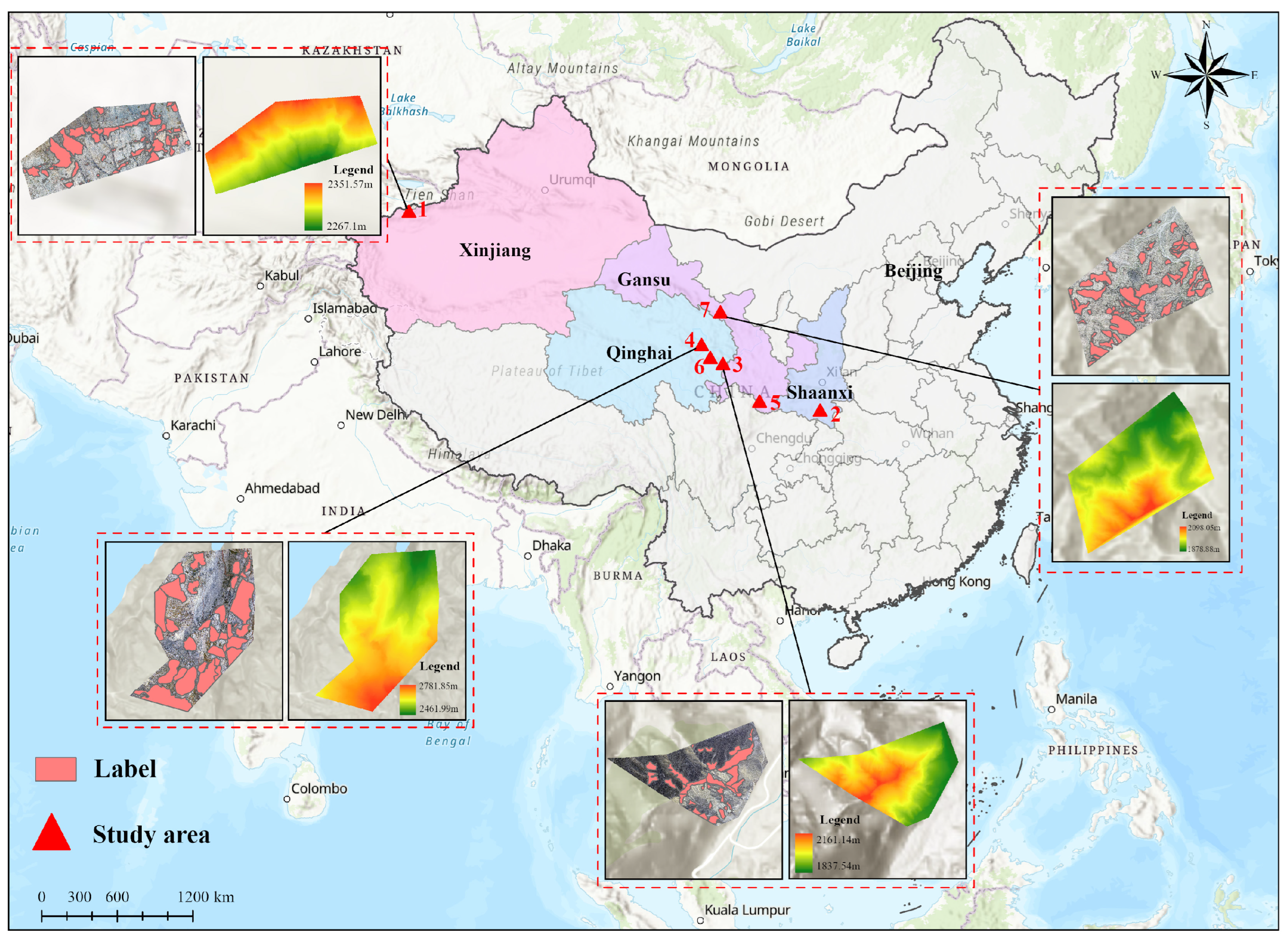
Seven typical hydropower engineering areas were selected for this study, including water conservancy hubs, hydropower stations, and pumped storage power stations: Daxiagu Water Conservancy Hub, Hanbin Pumped Storage Power Station, Jishixia Hydropower Station, Laxiwa Hydropower Station, Miaojia Dam Hydropower Station, Yangqu Hydropower Station, and Yongchang Pumped Storage Power Station. They are labeled with different numbers in Figure 2 and correspond to the descriptions below. These sites are distributed in typical mountainous regions of northwest and southwest China, covering Xinjiang, Shaanxi, Qinghai, and Gansu, and are highly representative of these areas.

• Daxiagu Water Conservancy Hub

Daxiagu Water Conservancy Hub is located in the Kumalak River gorge at the junction of Wensu County and Ushi County in Aksu Prefecture, Xinjiang, at 41.7°N and 78°E, representing a typical high-mountain canyon landform. The study area has a warm temperate arid climate, with low precipitation, high evaporation, and large diurnal temperature variation. The dam site valley shows a deep V-shaped profile, with steep slopes on both sides, sparse vegetation, and significant rock weathering. Local loose deposits and paleo-channel sediments are also developed, providing typical conditions for unstable rock mass formation.

2.

Hanbin Pumped Storage Power Station

Hanbin Pumped Storage Power Station is located in Yinghu Town, Hanbin District, Ankang City, Shaanxi Province, in the upper reaches of the Hanjiang River, at 32.7°N and 109.0°E. The study area has a humid subtropical climate with relatively abundant precipitation and strong seasonal variation. The terrain is dominated by mid- and low-mountain valleys, with higher elevations in the northwest and lower elevations in the southeast, and deeply incised river valleys. The power station adopts an integrated layout of a newly constructed upper reservoir and the Ankang Reservoir as the lower reservoir. The upper reservoir area is mainly composed of metamorphic rocks, with local loose deposits. The lower reservoir area is underlain by hard granite and sandstone. The region shows potential conditions for unstable rock mass distribution.

3.

Jishixia Hydropower Station

Jishixia Hydropower Station is located in the Jishixia reach of the upper Yellow River, at the boundary between Qinghai and Gansu Provinces, at 35.8°N and 102.7°E. The study area has a plateau continental climate, characterized by dry conditions, low precipitation, frequent strong winds, and a large diurnal temperature variation. The dam site valley is a deeply incised V-shaped canyon, with thick mountain masses and steep slopes on both sides. The bedrock is mainly composed of granite and gneiss, with relatively intact rock masses but well-developed joints, forming a typical high and steep rock slope environment.

4.

Laxiwa Hydropower Station

Laxiwa Hydropower Station is located in the Laxiwa gorge reach of the Yellow River in Qinghai Province, at the geomorphic transition zone from the Qinghai–Tibet Plateau to the Loess Plateau, at 36.0°N and 101.2°E. The study area has a plateau continental climate with dry conditions and large diurnal temperature variation, and the dam site valley is narrow with steep slopes (about 40–60°). The bedrock is mainly granite, with local unloading zones and loose deposits, and slope stability issues are prominent.

5.

Miaojia Dam Hydropower Station

Miaojia Dam Hydropower Station is located in the downstream reach of the Bailong River in Wen County, Gansu Province, at 32.9°N and 104.7°E, and is a mountain canyon-type reservoir. The study area lies in the transitional zone from a subtropical monsoon climate to a temperate climate, with precipitation concentrated in summer and strong seasonal variation in runoff. The reservoir channel is highly sinuous, and the slopes on both sides are mainly composed of metamorphic rocks and slate. Faults and joint fractures are well developed, and local colluvial deposits and small landslide bodies are present, resulting in relatively complex geological conditions.

6.

Yangqu Hydropower Station

Yangqu Hydropower Station is located at the boundary between Xinghai County and Guinan County in Qinghai Province along the upper Yellow River, at 35.6°N and 100.8°E, with an elevation above 3000 m, representing a typical plateau canyon landform. The study area has long sunshine duration, cold and long winters, and high evaporation. The dam site is located in a narrow reach of the Yangqu gorge, with low vegetation coverage on the surrounding mountains. The slopes on both sides are mainly rock slopes with well-developed joints and fractures, and local weathered layers and loose deposits are present.

7.

Yongchang Pumped Storage Power Station

Yongchang Pumped Storage Power Station is located on the northern foothills of the Qilian Mountains in Yongchang County, Gansu Province, at 38.2°N and 102.0°E, within the mountain canyon region of the Hexi Corridor. The study area belongs to the Xida River system of the Shiyang River basin, where precipitation is concentrated from June to September, accounting for more than 70% of the annual total. Floods are mainly rainstorm-induced, with a high peak, low volume, and short duration. The terrain is highly undulating with well-developed valleys. The rock mass is relatively intact with a thin weathered layer, and local small-scale loose deposits are present.

Figure 2 shows the spatial distribution of the seven study areas, all of which are marked by red symbols. Due to layout limitations, four representative areas are enlarged for visual illustration. The selected regions are mostly located in high-mountain canyon areas with strong topographic relief and steep slopes. The rock masses are strongly affected by tectonic and weathering processes, and unstable rock masses are widely developed with diverse types. These areas are ideal for the remote sensing-based detection of unstable rock masses in complex surface environments. In addition, the introduction of multiple regions and engineering scenarios helps build a dataset with good generalization ability, thereby improving the applicability and robustness of the model under different terrain conditions.

3.1.2. Production of Sample Database

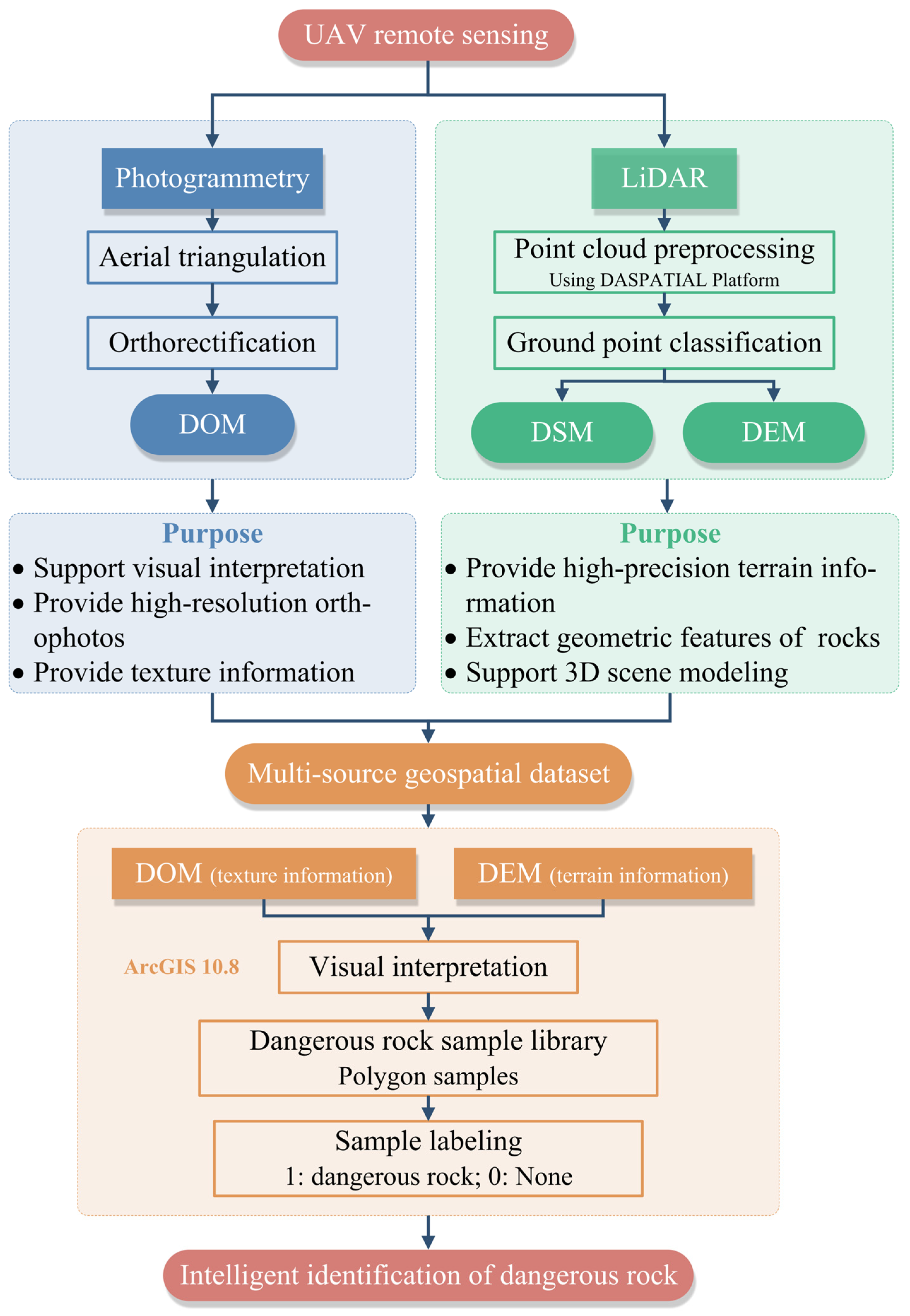
UAV RGB images and LiDAR point cloud data were acquired over seven study regions and processed using the DASpatial platform. UAV images were corrected and orthorectified to generate the RGB DOM, while LiDAR point clouds were preprocessed through trajectory correction, registration, noise filtering, and ground-point classification. Ground points were then extracted and interpolated to generate the DEM, which was co-registered with the RGB DOM to ensure spatial consistency. The UAV RGB DOM has a spatial resolution of 0.5 m, while the DEM has a spatial resolution of 0.5 m. A DSM was used only for DOM orthorectification during UAV photogrammetric preprocessing and was not used as a model input or involved in sample generation. The data acquisition and processing workflow is shown in Figure 3.

Unstable rock mass annotations were produced through manual visual interpretation in ArcGIS 10.8 based on the high-resolution RGB DOM and typical spectral, textural, and morphological features of unstable rock masses. The boundaries of unstable rock masses were vectorized to generate binary labels, where unstable rock mass pixels were assigned a value of 1 and background pixels were assigned a value of 0. To improve annotation consistency, a multi-person cross-interpretation and consistency checking strategy was adopted. Ambiguous or inconsistent boundaries were re-examined and corrected to reduce subjective interpretation errors.

In the data preprocessing and sample construction process, multi-source data were jointly processed, and standardized samples were generated. Supervised deep learning models rely heavily on well-annotated datasets. However, the considerable variation in the spatial scale of unstable rock masses poses a challenge when determining a universal patch size for model training. Drawing upon established practices in deep learning-based geohazard detection [26,51,52,53], a uniform sliding window of 256 × 256 pixels was adopted to systematically traverse and crop the study area. The complete dataset, including negative samples (256 × 256 pixels), was divided into training, validation, and test sets at a ratio of 6:2:2. Specifically, samples from each of the seven study regions were independently split into training, validation, and test subsets using the same ratio, so that all subsets contained samples from each region. Each cropped patch was assigned a unique identifier according to its region and spatial position, and duplicate checking was performed to ensure that no identical patch appeared in more than one subset. However, because the samples were generated using a sliding-window strategy, adjacent patches from the same unstable rock mass may still share a similar spatial context. Therefore, the current evaluation should be interpreted as patch-level performance on a multi-region dataset rather than strict site-disjoint generalization.

3.2. Experimental Setup

All experiments were conducted on a Windows 11 workstation equipped with an NVIDIA GeForce RTX 4090 GPU with 24 GB of memory. All models were implemented using PyTorch v2.1.1 and accelerated with CUDA 11.8. The training process was set to 100 epochs, with a batch size of 8. The input remote sensing images were normalized to a size of 4 × 256 × 256, and stochastic gradient descent (SGD) [54] was used for optimization. Based on preliminary empirical tests with different initial learning rates ranging from 1 × 10⁻¹ to 1 × 10⁻⁵, the optimal initial learning rate was set to 1 × 10⁻⁴. To improve model convergence, a ReduceLROnPlateau scheduler was adopted to implement a dynamic learning rate decay strategy. Specifically, if the training metric did not improve for 10 consecutive epochs, the learning rate was reduced by 20%, that is, multiplied by 0.8. In unstable rock mass detection tasks, the dataset is highly imbalanced, and positive samples usually account for only a small proportion of the overall data. This imbalanced distribution can cause the model to be biased toward the majority class, namely the background class, since optimizing background features can more easily reduce the overall loss. Although this may result in apparently high overall accuracy, it weakens the model’s ability to detect the minority class of interest. To address this issue, a boundary loss function was introduced to improve the segmentation performance of GTSNet [55]. The measured inference latency and peak memory usage are further reported in Section 3.5.

3.3. Comparison with Different Inputs and Methods

To comprehensively evaluate the effectiveness and superiority of the proposed GTSNet for unstable rock mass detection, we conducted quantitative comparison experiments with six common deep learning semantic segmentation networks (HFENet [56], ESANet [57], CMFNet [58], ASMFNet [59], PSPNet [60], and Swin Transformer [61]). All models were trained and tested under the same hardware and software environment and identical hyperparameter settings to ensure a fair comparison. Quantitative evaluation was conducted using five core metrics: overall accuracy (Acc), F1-score (F1), intersection over union (IoU), Precision (P), and Recall (R).

As shown in

Table 2. Quantitative comparison of different models under RGB-only, DEM-only, and RGB+DEM input settings (unit: %).

Model	Input	Acc	F1	IoU	P	R
HFENet	DEM	79.67	50.69	33.95	49.45	51.99
	RGB	83.70	58.07	40.91	60.14	56.13
	RGB+DEM	79.45	62	44.93	49.34	83.38
ESANet	DEM	83.41	55.09	38.02	60.41	50.63
	RGB	85.55	61.34	44.23	66.36	57.02
	RGB+DEM	84.9	69.83	53.64	58.36	86.9
CMFNet	DEM	60.25	46.94	30.67	32.08	87.47
	RGB	86.86	67.22	50.63	67.43	67.02
	RGB+DEM	89.4	73.75	58.41	73.42	74.09
ASMFNet	DEM	78.80	43.61	27.88	46.86	40.78
	RGB	83.59	61.36	44.26	58.25	64.83
	RGB+DEM	86.59	67.90	51.40	65.41	70.59
PSPNet	DEM	32.32	35.84	21.83	22.14	94.04
	RGB	75.26	59.17	42.01	44.27	89.20
	RGB+DEM	78.51	62.38	45.33	48.13	88.64
Swin Transformer	DEM	36.18	38.58	23.90	23.91	99.70
	RGB	84.06	68.99	52.66	56.64	88.24
	RGB+DEM	84.15	69.98	53.83	56.5	91.93
GTSNet (ours)	DEM	73.33	58.11	40.96	42.46	92.04
	RGB	88.62	71.14	55.20	72.58	69.76
	RGB+DEM	90.14	75.75	60.97	74.87	76.66

, for all compared models, the RGB + DEM input achieves higher F1-score and IoU than either the DEM-only or RGB-only input. Specifically, compared with the RGB-only input, the IoU values of HFENet, ESANet, CMFNet, ASMFNet, PSPNet, Swin Transformer, and GTSNet increase by 4.02%, 9.41%, 7.78%, 7.14%, 3.32%, 1.17%, and 5.77%, respectively. Compared with DEM-only input, the corresponding IoU improvements are 10.98%, 15.62%, 27.74%, 23.52%, 23.50%, 29.93%, and 20.01%, respectively. These consistent improvements indicate that RGB imagery and DEM provide complementary information for unstable rock mass segmentation. RGB imagery mainly contributes spectral, textural, and surface appearance information, while DEM provides terrain-related geometric cues associated with elevation variations. Therefore, the improvement obtained by RGB + DEM should first be interpreted as the benefit of multi-modal information integration rather than as the contribution of a specific network alone.

The comparison between DEM-only and RGB-only inputs further shows that the two modalities provide different but incomplete information. DEM-only input can provide terrain-related information, but it lacks detailed surface texture and spectral characteristics. As a result, several DEM-only models show relatively low Precision but high Recall, such as PSPNet and Swin Transformer, indicating a tendency toward over-detection. RGB-only input generally achieves better target delineation than DEM-only input because optical imagery contains richer visual appearance features. However, RGB-only models may still be affected by shadows, exposed bedrock, gravel surfaces, and visually similar backgrounds. These results explain why combining RGB and DEM generally leads to better target-level segmentation performance than using either modality alone. Under the same RGB+DEM input condition, GTSNet achieves the highest overall performance among the compared models, with an Acc of 90.14%, an F1-score of 75.75%, and an IoU of 60.97%. Considering the severe class imbalance in unstable rock mass detection, IoU and F1-score are more informative than overall accuracy for evaluating target-level segmentation performance. Compared with the second-best model CMFNet, GTSNet improves IoU by 2.56% and F1-score by 2.00%. Compared with the Swin Transformer baseline, GTSNet improves IoU by 7.14% and F1-score by 5.77%. Since all models are evaluated using the same RGB+DEM input, these improvements should not be attributed to DEM alone, but are more reasonably associated with the proposed network architecture, including global context modeling and topography-aware feature fusion.

Further analysis of Precision and Recall shows that some comparison models exhibit an imbalanced prediction tendency under the RGB + DEM setting. For example, PSPNet and Swin Transformer achieve high Recall values of 88.64% and 91.93%, respectively, but their Precision values are only 48.13% and 56.50%. This indicates that these models tend to detect more candidate target regions while introducing more false positives. In contrast, GTSNet obtains a Precision of 74.87% and a Recall of 76.66%, showing a more balanced Precision–Recall performance under the tested condition. This result suggests that GTSNet can better exploit the complementary information between RGB imagery and DEM, thereby reducing background confusion while maintaining a reasonable target detection capability.

Further analysis of Precision and Recall shows that some comparison models exhibited an imbalanced prediction tendency. For example, Swin Transformer and PSPNet achieved relatively high Recall values of 91.93% and 88.64%, respectively, but their Precision values were only 56.50% and 48.13%. This indicates that these models tend to detect more candidate target regions while introducing more false positives, such as exposed bedrock, mountain shadows, and engineering-disturbed slopes. In contrast, GTSNet obtained a Precision of 74.87% and a Recall of 76.66%, showing a more balanced Precision–Recall performance under the tested conditions. This suggests that GTSNet can better suppress background interference from visually similar non-target regions while maintaining a reasonable detection rate.

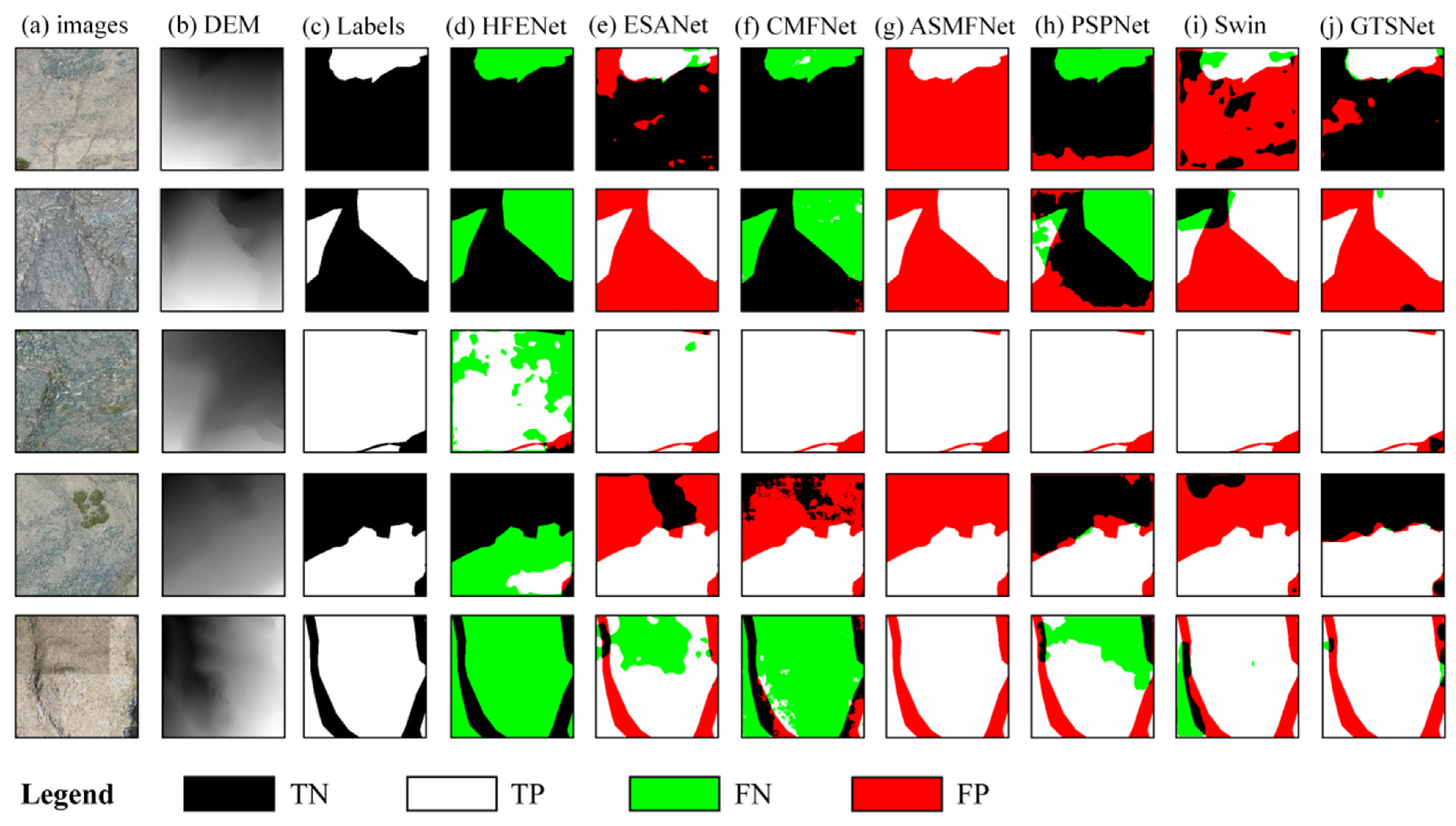
Figure 4 intuitively shows the segmentation prediction masks of the proposed GTSNet and six other segmentation models under typical complex geological scenes. Through visualization analysis of the spatial distribution of true positives (TP, white), true negatives (TN, black), false positives (FP, red), and false negatives (FN, green), the intrinsic differences in feature extraction and spatial boundary constraint ability among different models can be further examined. From an overall visual perspective, existing segmentation networks generally exhibit two extreme error tendencies when dealing with complex unstable rock mass detection: severe feature omission or overly aggressive over-segmentation.

On the one hand, HFENet, CMFNet, and PSPNet in some cases show clear limitations in feature representation, leading to significant omission errors (i.e., large green FN regions in the prediction maps). For example, in the second-row and fifth-row samples in Figure 4, the target unstable rock masses and surrounding non-target surfaces (such as normal rock–vegetation transition zones) exhibit highly similar spectral and texture features. In these cases, HFENet and CMFNet fail to extract sufficiently discriminative high-level semantic features and incorrectly classify large areas of true unstable rock masses as background. This conservative prediction behavior indicates that traditional shallow networks struggle to separate targets in complex terrain, and the high miss rate seriously limits their practical applicability in geological hazard monitoring.

On the other hand, ESANet, ASMFNet, and the baseline Swin model suffer from severe over-detection (i.e., many red FP regions in the images). As shown in the first, second, and fourth rows of Figure 4, when bare soil, slope shadows, or geological structures with similar shapes to fracture surfaces appear in the background, these models show very high sensitivity but poor robustness to interference, incorrectly identifying large areas of safe background as unstable rock masses. This qualitative observation is consistent with the quantitative results discussed above, where these models exhibit high Recall and low Precision, further confirming that they lack effective spatial contextual constraints to suppress background noise caused by complex geomorphic conditions.

3.4. Ablation Studies of GTSNet Components

To further verify the contributions of the key components in the proposed GTSNet architecture, a series of ablation experiments was conducted, using Acc, F1, IoU, P, and R as evaluation metrics. The performance gains of the Multi-scale Topography-Aware Module (Fusion) and the Transformer-based backbone encoder (Backbone) were systematically isolated and quantified and the quantitative ablation results are shown in

Table 3. Ablation results of GTSNet on the unstable rock mass dataset.

DEM	Fusion	Backbone	Acc	F1	IoU	P	R
✓	✗	✗	89.36	72.72	57.13	75	70.57
✓	✗	✓	89.29	73.37	57.94	73.36	73.38
✓	✓	✗	89.39	73.61	58.24	73.6	73.62
✓	✓	✓	90.14	75.75	60.97	74.87	76.66

. The following analysis discusses the effectiveness of each module from two perspectives based on the experimental results.

3.4.1. Spatial Refinement Ability of the Topography-Aware Fusion Module

In remote sensing image segmentation, high-level semantic feature extraction often leads to the loss of spatial details, which may cause boundary ambiguity or fragmented predictions when dealing with unstable rock masses with irregular shapes. To evaluate the contribution of the proposed Topography-aware Fusion Module, controlled ablation experiments were conducted by comparing model variants with and without the fusion module under the same input settings.

As shown in Table 3, when the Transformer backbone is used but the fusion module is removed, the model achieves an IoU of 57.94% and an F1-score of 73.37%. After introducing the proposed fusion module, the IoU increases to 60.97%, and the F1-score improves to 75.75%. Precision and Recall also increase from 73.36% and 73.38% to 74.87% and 76.66%, respectively. These results suggest that the fusion module contributes to improving target-level segmentation performance, especially in terms of boundary delineation and target completeness. A similar trend can also be observed when the Transformer backbone is not used. Compared to the model without the fusion module, introducing the fusion module increases the IoU from 57.13% to 58.24% and the F1-score from 72.72% to 73.61%, indicating that the proposed fusion module can still provide useful multi-scale feature refinement in a CNN-based architecture. Overall, the ablation results suggest that the Topography-aware Fusion Module helps integrate high-level terrain-semantic information with low-level spatial details, thereby improving the segmentation of unstable rock masses under complex geomorphic backgrounds.

3.4.2. Contribution of the Transformer Backbone

To evaluate the contribution of the Transformer backbone to global contextual representation, we further compared the model variants with and without the Transformer backbone, as shown in Table 3. When the Topography-aware Fusion Module is not used, introducing the Transformer backbone increases the IoU from 57.13% to 57.94% and the F1-score from 72.72% to 73.37%. Recall also increases from 70.57% to 73.38%, suggesting that the Transformer backbone helps the model capture more target-related regions by introducing broader contextual information.

When the Topography-aware Fusion Module is included, the contribution of the Transformer backbone becomes more evident. Compared with the model without the Transformer backbone, the complete model improves the IoU from 58.24% to 60.97% and the F1-score from 73.61% to 75.75%. Precision and Recall also increase from 73.60% and 73.62% to 74.87% and 76.66%, respectively. This result indicates that the high-level contextual features extracted by the Transformer backbone can provide useful semantic guidance for the subsequent topography-aware fusion process.

Overall, the Transformer backbone contributes to unstable rock mass segmentation by enhancing global contextual representation. Local texture information alone is often insufficient for distinguishing unstable rock masses from visually similar backgrounds, such as exposed bedrock, slope shadows, and engineering-disturbed surfaces. By modeling long-range dependencies, the Transformer backbone provides more stable high-level semantic information. Its effect is further strengthened when combined with the Topography-aware Fusion Module, indicating that global context modeling and multi-scale feature refinement are complementary in GTSNet.

3.4.3. Ablation Study on Transformer Placement

To further examine the influence of Transformer placement on unstable rock mass segmentation, an additional ablation experiment was conducted under the same RGB+DEM input, training strategy, loss function, and Topography-aware Fusion Module settings. Four model variants were compared: CNN-only + Fusion, GTSNet-S3, GTSNet-S4, and GTSNet-S3+S4. Here, GTSNet-S3, GTSNet-S4, and GTSNet-S3+S4 denote variants in which the Transformer block is placed at Stage 3, Stage 4, and both Stage 3 and Stage 4, respectively. The CNN-only + Fusion variant was used as the no-Transformer baseline, and GTSNet-S4 corresponds to the final configuration adopted in this study. According to the results shown in

Table 4. Ablation study on Transformer placement in GTSNet.

Model Variant	Transformer Placement	Acc	F1	IoU	P	R
CNN-only + Fusion	None	89.39	73.61	58.24	73.6	73.62
GTSNet-S3	Stage 3	87.91	70.85	54.86	68.72	73.12
GTSNet-S4	Stage 4	90.14	75.75	60.97	74.87	76.66
GTSNet-S3+S4	Stage 3 + Stage 4	88.80	72.21	56.51	72.24	72.39

, the CNN-only + Fusion variant achieves an Acc of 89.39%, an F1-score of 73.61%, and an IoU of 58.24%. When the Transformer is placed at Stage 3 only, GTSNet-S3 obtains an Acc of 87.91%, an F1-score of 70.85%, and an IoU of 54.86%, which are lower than those of the CNN-only + Fusion baseline. This indicates that introducing the Transformer at an intermediate feature stage does not improve segmentation performance in the current framework. A possible reason is that Stage 3 features still retain relatively rich local spatial details and background textures, and applying global self-attention at this stage may weaken boundary-related local information or introduce redundant contextual responses.

In contrast, when the Transformer is placed at Stage 4 only, GTSNet-S4 achieves the best performance among the tested variants, with an Acc of 90.14%, an F1-score of 75.75%, and an IoU of 60.97%. Compared with the CNN-only + Fusion baseline, GTSNet-S4 improves the F1-score by 2.14% and the IoU by 2.73%. This result suggests that Stage 4 is more suitable for Transformer-based global context modeling because the features at this stage contain more abstract semantic information and have a larger receptive field. Therefore, the Transformer can provide high-level contextual guidance for the subsequent topography-aware feature fusion process.

When Transformers are placed at both Stage 3 and Stage 4, GTSNet-S3 + S4 obtains an Acc of 88.80%, an F1-score of 72.21%, and an IoU of 56.51%, which are still lower than those of GTSNet-S4. This result suggests that adding an additional Transformer at Stage 3 does not bring further improvement and may instead introduce redundant global responses or increase optimization difficulty. Therefore, the Stage 4-only placement was adopted in the final GTSNet because it provides the most favorable segmentation performance among the tested Transformer placement strategies.

3.4.4. Qualitative Visualization of the Feature Fusion Process

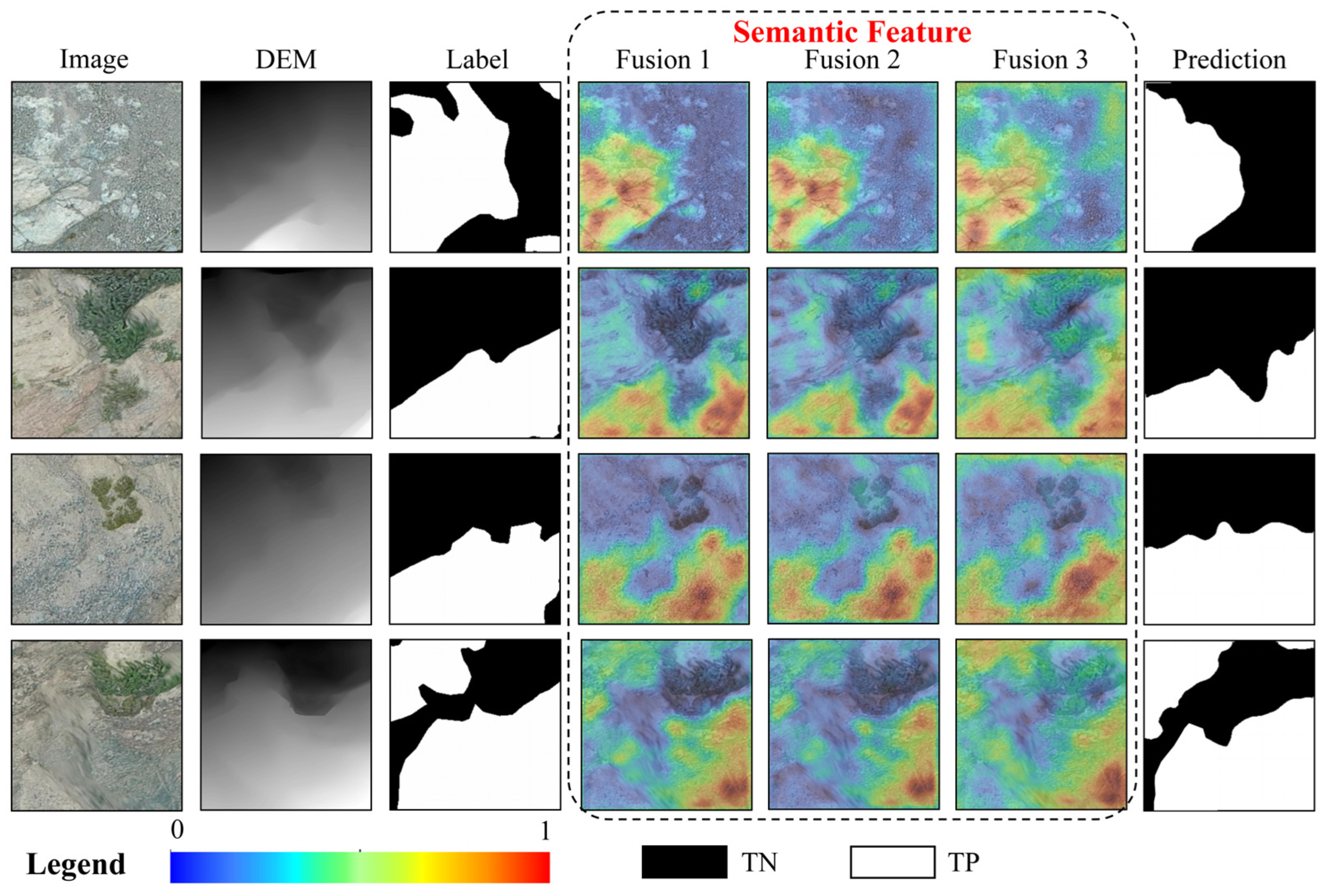
To further interpret the feature fusion process, Class Activation Mapping (CAM) [62] was used to visualize the intermediate responses of different fusion stages, as shown in Figure 5. It should be noted that CAM is only used as a qualitative visualization tool and does not participate in feature fusion or model training. In the heatmaps, red regions indicate higher activation responses, while blue regions indicate lower responses. The Fusion 1 heatmap mainly reflects high-level semantic responses from deeper features and broadly covers potential target regions. However, due to the relatively low spatial resolution of deep features, the activated regions remain coarse and may include adjacent background areas.

In Fusion 2, the activation responses become more concentrated after incorporating mid-level features. Compared with Fusion 1, the highlighted regions show better consistency with terrain-related boundary cues. Since the network uses the raw DEM as input rather than explicitly derived slope, gradient, or curvature products, these responses should be interpreted as data-driven terrain-related features learned from DEM-derived elevation variations. These results suggest that DEM information may help reduce the interference caused by homogeneous optical appearances, such as bare soil, gravel surfaces, and slope shadows.

In Fusion 3, high-resolution shallow features are further introduced, and the activation responses become more spatially refined. The highlighted regions are more concentrated around unstable rock mass areas, indicating that the fusion process gradually shifts from coarse semantic localization to finer boundary representation. These CAM results are used only as qualitative visualization and should be interpreted together with the quantitative ablation results in Table 3.

3.5. Model Complexity and Deployment Efficiency Analysis

To comprehensively evaluate the practical application potential of different networks, we compared both model complexity and deployment-relevant inference efficiency. In addition to parameter count and floating-point operations, per-image inference latency and peak GPU memory usage were measured, as these metrics provide more direct evidence for practical deployment. All measurements were conducted on the same NVIDIA GeForce RTX 4090 GPU with a batch size of 1 and an input size of 4 × 256 × 256. The latency was calculated as the average inference time per image after GPU warm-up, and the peak memory usage was recorded during inference. The results are shown in

Table 5. Model complexity and deployment efficiency of the compared networks.

Models	Params (M)	Flops (G)	Latency (ms/Image)	Peak Memory (MB)
HFENet	21.28	32.63	11.09	231.25
ESANet	23.92	5.21	14.91	237.69
CMFNet	98.49	78.33	36.48	801.11
ASMFNet	80.46	17.93	23.24	742.65
PSPNet	17.42	27.48	13.45	708.07
Swin Transformer	27.95	5.84	15.06	258.93
GTSNet	28.26	52.13	14.47	295.58

.

According to the results shown in Table 5, GTSNet contains 28.26 M parameters and requires 52.13 G FLOPs, with an inference latency of 14.47 ms/image and a peak GPU memory usage of 295.58 MB. Compared with high-parameter models such as CMFNet and ASMFNet, GTSNet has a much smaller parameter size. Specifically, the number of parameters is reduced by approximately 71.3% compared with CMFNet and 64.9% compared with ASMFNet. In terms of memory usage, GTSNet also requires substantially less peak GPU memory than CMFNet, ASMFNet, and PSPNet. Although the FLOPs of GTSNet are not the lowest among the compared models, its inference latency remains within a range comparable to lightweight models such as ESANet and Swin Transformer. Meanwhile, GTSNet achieves a higher segmentation accuracy, F1-score, and IoU under the same experimental settings. Therefore, GTSNet provides a reasonable balance between segmentation performance and deployment efficiency for patch-based UAV image interpretation. For full-resolution UAV images, direct prediction for the entire image is usually limited by GPU memory because the original images are much larger than the network input size. Therefore, full-resolution inference was performed using a tile-based sliding-window strategy. Each full-resolution image was divided into 256 × 25,6256/times 25,6256 × 256 patches, and each patch was independently predicted by the trained model. The patch-level prediction results were then mosaicked back to the original spatial extent to generate the final unstable rock mass map. Under this strategy, the total inference time depends mainly on the image size and the number of generated patches, while the per-patch latency reported in Table 5 provides a basis for estimating full-resolution inference efficiency.

4. Discussion

4.1. Effectiveness Analysis of DEM Multi-Modal Features on Spatial Topological Constraints

To quantitatively evaluate the contribution of the DEM in complex geological environments, we performed a comparative analysis using a baseline version of GTSNet that relies solely on optical imagery. As shown in

Table 6. Ablation study on the impact of DEM spatial constraints and data augmentation strategies on network segmentation performance.

Metrics	Acc	F1	IoU	P	R
RGB	88.6	70.65	54.62	73.21	68.27
RGB + DEM	90.14	75.75	60.97	74.87	76.66

, without incorporating the DEM, GTSNet achieves an IoU of only 54.62% and an F1-score of 70.65%. Under the same GTSNet architecture, the introduction of the DEM improved the model performance: specifically, the IoU increased from 54.62% to 60.97%, the F1-score increased from 70.65% to 75.75%, and the Recall increased from 68.27% to 76.66%. These results suggest that DEM information may provide complementary terrain-related geometric cues to optical imagery.

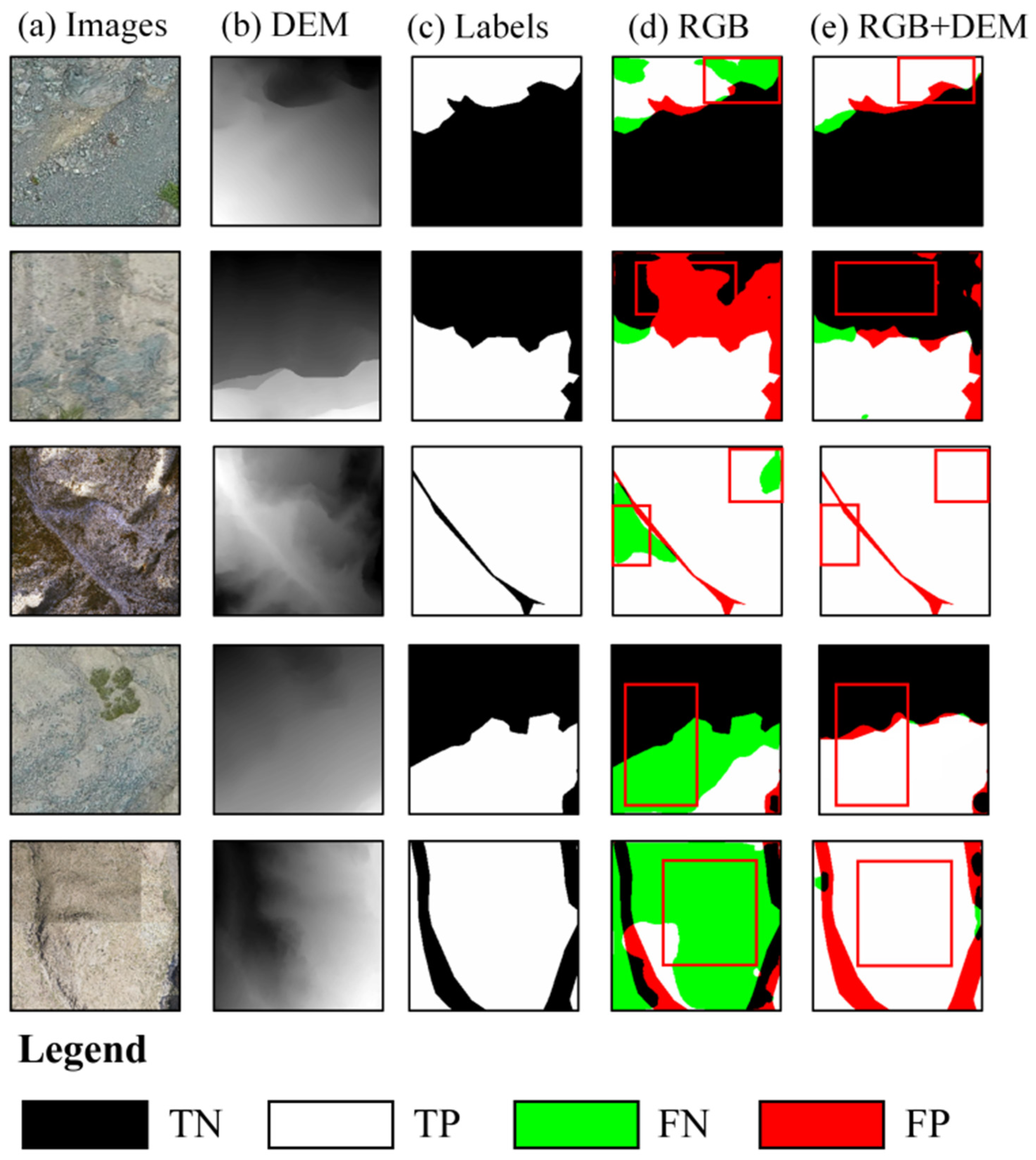
To intuitively and comprehensively evaluate the effectiveness of multi-modal data fusion, Figure 6 presents a visual comparison between two models—one relying solely on optical imagery (RGB) and the other incorporating elevation data (RGB+DEM)—under typical and highly challenging geological scenarios. In the figure, the red boxes highlight regions where significant differences in network performance are observed. Green indicates FN, while red indicates FP. It is worth noting that in the DEM visualization, darker pixels represent higher elevation, whereas lighter pixels correspond to lower elevation.

First, the elevation information provided by the DEM substantially reduces FP (red regions) caused by homogeneous textures. As shown in the second-row and third-row samples, the optical images in column (a) exhibit highly similar gravel or rock–soil textures between targets and backgrounds. As a result, the original GTSNet without DEM integration produces a large number of false positive regions in column (d), such as the extensive red areas in the upper-right part of the second row. However, the DEM data in column (b) show that the misclassified background regions appear darker (indicating higher elevation), whereas the actual sliding surfaces or target regions appear lighter (indicating lower-lying or stepped terrain areas). After integrating the DEM, GTSNet effectively captures this sharp elevation transition from dark to light and successfully removes the misclassified regions within the red boxes in column (e), converting them into correctly classified background areas (black, TN). As a result, the predicted boundaries closely align with the actual terrain.

DEM-derived topographic features effectively alleviate FN (green regions) caused by surface camouflage. In complex field environments, vegetation cover, shadows, or uneven illumination can easily disrupt the continuity of visual features. As shown in the fourth-row sample, obvious green vegetation patches appear in the center of the optical image, causing the original GTSNet to be disturbed by visual noise and produce severe false negative regions within the red box in column (d). However, in the corresponding DEM image, the elevation variation in this region shows a smooth transition, indicating that the area beneath the vegetation belongs to a continuous geological body. In column (e), the originally missed green regions are successfully restored to white regions representing TP. The fifth-row sample is more representative. Strong shadows and abrupt soil variations in the RGB image cause the RGB-based model to almost completely miss the core target region, resulting in large FN areas (green). In contrast, the DEM image clearly delineates a typical valley structure with dark regions on both sides (high elevation) and a bright region in the center (low elevation). Guided by this strong geometric prior, the prediction result in the red box of column (e) successfully reconstructs the target region.

The DEM not only provides the network with an additional dimension independent of optical imagery, but more importantly, the elevation distribution offers indispensable geomorphological interpretation for unstable rock mass boundaries. The deep collaboration between optical features and elevation data therefore enables effective scene understanding in highly complex real geological environments.

4.2. Effectiveness Evaluation of the Data Augmentation Strategy

In intelligent identification tasks for complex geological targets driven by multi-source remote sensing data, such as landslides and unstable rock masses, deep learning models often face multiple challenges, including the scarcity of high-quality labeled samples, large intra-class geomorphic variability, and strong background interference. In particular, in upstream basins or mountainous canyon regions with dramatic terrain fluctuations, limited samples can easily increase the risk of overfitting. In this section, to address this issue and further evaluate the effect of data augmentation on GTSNet, we analyze the performance changes before and after applying augmentation strategies. During training, data augmentation was applied to increase sample diversity and reduce overfitting. The spatial geometric transformations included random horizontal flipping, random vertical flipping, random rotation, and random scaling/cropping. The radiometric perturbations included random brightness adjustment, random contrast adjustment, and noise perturbation. All augmentation operations were applied only to the training set, while the validation and test sets were kept unchanged.

Table 7. Comparison of model recognition performance before and after data augmentation.

Metrics	Acc	F1	IoU	P	R
Before data augmentation	90.14	75.75	60.97	74.87	76.66
After data augmentation	90.82	77.29	62.98	76.86	77.72

presents a detailed comparison of all evaluation metrics between the original GTSNet and the model trained with data augmentation.

From an overall performance perspective, the introduction of data augmentation improves the model’s performance under the current experimental settings: specifically, the IoU increases from 60.97% to 62.98%, with a gain of 2.01%, while the F1-score rises from 75.75% to 77.29%. These results suggest that augmentation strategies, such as spatial geometric transformations and radiometric perturbations, can enlarge the effective distribution of the training data and reduce the risk of overfitting. By exposing the model to more diverse spatial and radiometric variations, data augmentation may help the network learn more robust feature representations, thereby improving its adaptability to complex terrain scenarios.

A detailed analysis of the evaluation metrics in Table 7 shows that Precision increases from 74.87% to 76.86%. In unstable rock mass interpretation, higher Precision indicates that the model produces fewer false positive predictions, suggesting a reduced tendency to misclassify visually similar background areas, such as exposed rock–soil surfaces or non-hazardous slopes, as target hazard objects. Meanwhile, Recall also increases from 76.66% to 77.72%, indicating that the model maintains or slightly improves its sensitivity to unstable rock mass targets while reducing false detections.

4.3. Limitations and Future Work

Although the proposed GTSNet achieves significant performance in fusing optical imagery and DEM elevation data, effectively mitigating visual interference in complex terrains and enabling fine-grained unstable rock mass segmentation, this study still has certain limitations in terms of the dynamic evolution of data modalities and computational cost during model deployment.

First, while the current network architecture mainly relies on static optical imagery from a specific time phase and a DEM for spatial feature extraction, the initiation and evolution of geological hazards are highly complex spatiotemporal dynamic processes. Although static topographic and textural features can effectively identify already existing or morphologically distinct hazard bodies, they remain insufficient for capturing subtle deformation precursors prior to hazard occurrence. Second, at the architectural level, although the introduction of the Transformer module endows the network with strong global context modeling capability, the computational complexity of its self-attention mechanism increases quadratically with the input resolution. When processing large-scale remote sensing imagery in upstream basins or extensive transportation corridors, this imposes considerable demands on computational resources, particularly GPU memory, which to some extent limits frequent large-area real-time deployment of the model on edge devices or in geological disaster emergency response scenarios.

To address the above limitations, future research will focus on the following two key directions to further enhance hazard perception capabilities in complex geological environments.

(1)

Although the duplicate-checking procedure confirmed that no identical cropped image patch appeared in more than one subset, the current dataset was randomly split at the patch level rather than by strict geographic site separation. Therefore, spatially adjacent patches from the same unstable rock mass or the same engineering site may still exist in different subsets, which may introduce spatial correlation and result in a relatively optimistic performance estimation. Future work will further adopt site-level hold-out validation or spatial block-based cross-validation to more rigorously evaluate the geographic transferability and cross-site generalization ability of GTSNet.

(2)

Introduction of multi-source temporal remote sensing and a dynamic susceptibility evaluation mechanism: Future research will surpass the limitations of static imagery and focus on the deep integration of temporal optical imagery and InSAR technology, which has a millimeter-level ground deformation monitoring capability. By constructing a 3D spatiotemporal multi-source fusion framework combining “temporal optical appearance features + DEM static foundation + InSAR dynamic deformation features”, the network can not only identify the boundaries of unstable rock masses but also quantitatively extract the temporal deformation characteristics of landslides and unstable rock masses. Based on this multi-source temporal perception framework, the research focus will shift from single “unstable rock mass detection” to “dynamic susceptibility evaluation of unstable rock masses”, thereby providing more forward-looking scientific support for early warning and dynamic risk assessment of geological hazards in complex high-mountain canyon areas and along major engineering corridors.

(3)

Exploration of model lightweighting and vision foundation model-based zero-shot boundary refinement: To alleviate high computational costs and reduce dependence on large-scale pixel-level annotated data, future work will explore the introduction of lightweight backbone networks with spatial–channel joint attention mechanisms to replace part of the redundant convolutional layers. In addition, given the strong segmentation generalization capability demonstrated by general vision foundation models (such as the Segment Anything Model, SAM) on large-scale datasets, future work will explore a prompt-driven adapter mechanism that uses the coarse-grained semantic features output by GTSNet as spatial prompts to be fed into the SAM model. Leveraging the zero-shot boundary refinement capability of large models, the micro-topological edges of geological targets can be further refined, thereby achieving further improvement in geomorphological feature extraction accuracy while ensuring lightweight model deployment.

5. Conclusions

China is one of the countries most frequently affected by geological hazards in the world. Among these hazards, unstable rock masses in high-mountain canyon hydropower engineering areas are highly unpredictable and destructive; once destabilized, they pose serious threats to surrounding residents and to the long-term safe operation of major engineering infrastructures. To address the issues of missed detection and over-segmentation in traditional remote sensing interpretation and single optical features under complex terrain, shadow occlusion, and blurred object boundaries, we have proposed and developed a dual-modal deep learning framework—the Global Topography-aware Segmentation Network (GTSNet)—that integrates high-resolution UAV optical imagery and a DEM. The model combines CNN-based encoders for local detail extraction with the global representation capability of Transformer architectures, and introduces an innovative multi-scale Topography-aware Fusion Module to achieve deep collaborative modeling of appearance textures and three-dimensional terrain constraints. Using a professional unstable rock mass dataset covering seven typical hydropower engineering regions in China, we conducted a comprehensive qualitative and quantitative evaluation of the proposed model.

• The network achieves an overall accuracy of 90.14% and an IoU of 60.97%, effectively overcoming the common “high Recall, low Precision” limitation of existing mainstream segmentation networks in complex geological scenarios and achieving a better balance between missed detections and false positives.
• The ablation results suggest that the performance improvement of GTSNet is associated with the combined contribution of DEM information, global context modeling, and the multi-scale Topography-aware Fusion Module. DEM-derived terrain cues may help alleviate the confusion caused by homogeneous textures and complex backgrounds, while data augmentation may improve robustness by increasing the diversity of training samples.
• By applying spatial and radiometric perturbation-based augmentation strategies, the training data distribution is effectively expanded, enabling the network to learn more invariant intrinsic features with respect to scale and rotation, further improving the IoU to 62.98%.
• To address the limitations of static features and high computational cost, future research will integrate InSAR technology to conduct a dynamic susceptibility evaluation of unstable rock masses and will explore lightweight architectures combined with vision foundation models (such as SAM) for large-scale real-time deployment and zero-shot boundary refinement.

References

1. Xu, Q.; Zhao, B.; Dai, K.; Dong, X.; Li, W.; Zhu, X.; Yang, Y.; Xiao, X.; Wang, X.; Huang, J.; et al. Remote Sensing for Landslide Investigations: A Progress Report from China. Eng. Geol. 2023, 321, 107156. [Google Scholar] [CrossRef] [Scilit]
2. Bubeck, A.; Wilkinson, M.; Roberts, G.P.; Cowie, P.A.; McCaffrey, K.J.W.; Phillips, R.; Sammonds, P. The Tectonic Geomorphology of Bedrock Scarps on Active Normal Faults in the Italian Apennines Mapped Using Combined Ground Penetrating Radar and Terrestrial Laser Scanning. Geomorphology 2015, 237, 38–51. [Google Scholar] [CrossRef] [Scilit]
3. Matasci, B.; Stock, G.M.; Jaboyedoff, M.; Carrea, D.; Collins, B.D.; Guérin, A.; Matasci, G.; Ravanel, L. Assessing Rockfall Susceptibility in Steep and Overhanging Slopes Using Three-Dimensional Analysis of Failure Mechanisms. Landslides 2018, 15, 859–878. [Google Scholar] [CrossRef] [Scilit]
4. Liu, C.; Bao, H.; Zhang, J.; Yang, J.; Dong, X. Quantitative Identification and Hazard Assessment of Potentially Unstable Rock Masses along Mountainous Transportation Corridors. Eng. Fail. Anal. 2026, 183, 110273. [Google Scholar] [CrossRef] [Scilit]
5. Casagli, N.; Intrieri, E.; Tofani, V.; Gigli, G.; Raspini, F. Landslide Detection, Monitoring and Prediction with Remote-Sensing Techniques. Nat. Rev. Earth Environ. 2023, 4, 51–64. [Google Scholar] [CrossRef] [Scilit]
6. Du, Y.; Xie, M. Indirect Method for the Quantitative Identification of Unstable Rock. Nat. Hazards 2022, 112, 1005–1012. [Google Scholar] [CrossRef] [Scilit]
7. Scaioni, M.; Longoni, L.; Melillo, V.; Papini, M. Remote Sensing for Landslide Investigations: An Overview of Recent Achievements and Perspectives. Remote Sens. 2014, 6, 9600–9652. [Google Scholar] [CrossRef] [Scilit]
8. Chen, B.; Maurer, J.; Gong, W. Applications of UAV in Landslide Research: A Review. Landslides 2025, 22, 3029–3048. [Google Scholar] [CrossRef] [Scilit]
9. Li, C.; Zhang, G.; Lei, T.; Gong, A. Quick Image-Processing Method of UAV without Control Points Data in Earthquake Disaster Area. Trans. Nonferrous Met. Soc. China 2011, 21, s523–s528. [Google Scholar] [CrossRef] [Scilit]
10. Lian, X.; Li, Z.; Yuan, H.; Liu, J.; Zhang, Y.; Liu, X.; Wu, Y. Rapid Identification of Landslide, Collapse and Crack Based on Low-Altitude Remote Sensing Image of UAV. J. Mt. Sci. 2020, 17, 2915–2928. [Google Scholar] [CrossRef] [Scilit]
11. Casagli, N.; Frodella, W.; Morelli, S.; Tofani, V.; Ciampalini, A.; Intrieri, E.; Raspini, F.; Rossi, G.; Tanteri, L.; Lu, P. Spaceborne, UAV and Ground-Based Remote Sensing Techniques for Landslide Mapping, Monitoring and Early Warning. Geoenviron. Disasters 2017, 4, 9. [Google Scholar] [CrossRef] [Scilit]
12. Lindner, G.; Schraml, K.; Mansberger, R.; Hübl, J. UAV Monitoring and Documentation of a Large Landslide. Appl. Geomat. 2016, 8, 1–11. [Google Scholar] [CrossRef] [Scilit]
13. Hu, S.; Qiu, H.; Wang, X.; Gao, Y.; Wang, N.; Wu, J.; Yang, D.; Cao, M. Acquiring High-Resolution Topography and Performing Spatial Analysis of Loess Landslides by Using Low-Cost UAVs. Landslides 2018, 15, 593–612. [Google Scholar] [CrossRef] [Scilit]
14. Nex, F.; Remondino, F. UAV for 3D Mapping Applications: A Review. Appl. Geomat. 2014, 6, 1–15. [Google Scholar] [CrossRef] [Scilit]
15. Gonzalez, D.; Patricio, M.A.; Berlanga, A.; Molina, J.M. A Convolutional Neural Network Model for Superresolution Enhancement of UAV Images. In Proceedings of the 2019 IEEE International Conference on Pervasive Computing and Communications Workshops (PerCom Workshops), Kyoto, Japan, 11–15 March 2019; pp. 992–997. [Google Scholar] [CrossRef] [Scilit]
16. Du, W.; Sheng, Q.; Fu, X.; Chen, J.; Zhou, Y. Extensions of the Two-Phase Double-Point Material Point Method to Simulate the Landslide-Induced Surge Process. Eng. Anal. Bound. Elem. 2021, 133, 362–375. [Google Scholar] [CrossRef] [Scilit]
17. Gojcic, Z.; Schmid, L.; Wieser, A. Dense 3D Displacement Vector Fields for Point Cloud-Based Landslide Monitoring. Landslides 2021, 18, 3821–3832. [Google Scholar] [CrossRef] [Scilit]
18. Zheng, X.; He, G.; Wang, S.; Wang, Y.; Wang, G.; Yang, Z.; Yu, J.; Wang, N. Comparison of Machine Learning Methods for Potential Active Landslide Hazards Identification with Multi-Source Data. Int. J. Geo-Inf. 2021, 10, 253. [Google Scholar] [CrossRef] [Scilit]
19. Wang, L.; Zhang, M.; Shen, X.; Shi, W. Landslide Mapping Using Multilevel-Feature-Enhancement Change Detection Network. IEEE J. Sel. Top. Appl. Earth Obs. Remote Sens. 2023, 16, 3599–3610. [Google Scholar] [CrossRef] [Scilit]
20. Liu, X.; Wang, H.; Jing, H.; Shao, A.; Wang, L. Research on Intelligent Identification of Rock Types Based on Faster R-CNN Method. IEEE Access 2020, 8, 21804–21812. [Google Scholar] [CrossRef] [Scilit]
21. Jin, C.; Wang, K.; Han, T.; Lu, Y.; Liu, A.; Liu, D. Segmentation of Ore and Waste Rocks in Borehole Images Using the Multi-Module Densely Connected U-Net. Comput. Geosci. 2022, 159, 105018. [Google Scholar] [CrossRef] [Scilit]
22. Li, L.; Zhou, T.; Wang, W.; Li, J.; Yang, Y. Deep Hierarchical Semantic Segmentation. In Proceedings of the 2022 IEEE/CVF Conference on Computer Vision and Pattern Recognition (CVPR), New Orleans, LA, USA, 19–20 June 2022; pp. 1236–1247. [Google Scholar]
23. Cheng, B.; Schwing, A.G.; Kirillov, A. Per-Pixel Classification Is Not All You Need for Semantic Segmentation. Adv. Neural Inf. Process. Syst. 2021, 34, 17864–17875. [Google Scholar] [CrossRef] [Scilit]
24. Chen, L.-C.; Zhu, Y.; Papandreou, G.; Schroff, F.; Adam, H. Encoder-Decoder with Atrous Separable Convolution for Semantic Image Segmentation. In Computer Vision—ECCV 2018; Ferrari, V., Hebert, M., Sminchisescu, C., Weiss, Y., Eds.; Lecture Notes in Computer Science; Springer International Publishing: Cham, Switzerland, 2018; Volume 11211, pp. 833–851. [Google Scholar] [CrossRef] [Scilit]
25. Liu, P.; Wei, Y.; Wang, Q.; Chen, Y.; Xie, J. Research on Post-Earthquake Landslide Extraction Algorithm Based on Improved U-Net Model. Remote Sens. 2020, 12, 894. [Google Scholar] [CrossRef] [Scilit]
26. Rukundo, O. Evaluation of Extra Pixel Interpolation with Mask Processing for Medical Image Segmentation with Deep Learning. Signal Image Video Process. 2024, 18, 7703–7710. [Google Scholar] [CrossRef] [Scilit]
27. Ge, Y.; Wang, H.; Liu, G.; Chen, Q.; Tang, H. Automated Identification of Rock Discontinuities from 3D Point Clouds Using a Convolutional Neural Network. Rock Mech. Rock Eng. 2025, 58, 3683–3700. [Google Scholar] [CrossRef] [Scilit]
28. Cheng, Z.; Gong, W.; Tang, H.; Juang, C.H.; Deng, Q.; Chen, J.; Ye, X. UAV Photogrammetry-Based Remote Sensing and Preliminary Assessment of the Behavior of a Landslide in Guizhou, China. Eng. Geol. 2021, 289, 106172. [Google Scholar] [CrossRef] [Scilit]
29. Menegoni, N.; Giordan, D.; Perotti, C. Reliability and Uncertainties of the Analysis of an Unstable Rock Slope Performed on RPAS Digital Outcrop Models: The Case of the Gallivaggio Landslide (Western Alps, Italy). Remote Sens. 2020, 12, 1635. [Google Scholar] [CrossRef] [Scilit]
30. Du, B.; Huang, W.; Ye, J.; Tong, B.; Yin, Y. A Deformable Dual-Branch Visual State-Space Network for Landslide Identification with Multi-Scale Recognition and Irregular Boundary Enhancement. Remote Sens. 2026, 18, 707. [Google Scholar] [CrossRef] [Scilit]
31. Wu, L.; Liu, R.; Ju, N.; Zhang, A.; Gou, J.; He, G.; Lei, Y. Landslide Mapping Based on a Hybrid CNN-Transformer Network and Deep Transfer Learning Using Remote Sensing Images with Topographic and Spectral Features. Int. J. Appl. Earth Obs. Geoinf. 2024, 126, 103612. [Google Scholar] [CrossRef] [Scilit]
32. Ural, S.; Hussain, E.; Shan, J. Building Population Mapping with Aerial Imagery and GIS Data. Int. J. Appl. Earth Obs. Geoinf. 2011, 13, 841–852. [Google Scholar] [CrossRef] [Scilit]
33. Martha, T.R.; Kerle, N.; Jetten, V.; Van Westen, C.J.; Kumar, K.V. Characterising Spectral, Spatial and Morphometric Properties of Landslides for Semi-Automatic Detection Using Object-Oriented Methods. Geomorphology 2010, 116, 24–36. [Google Scholar] [CrossRef] [Scilit]
34. Han, L.; Duan, P.; Liu, J.; Li, J. Research on Landslide Trace Recognition by Fusing UAV-Based LiDAR DEM Multi-Feature Information. Remote Sens. 2023, 15, 4755. [Google Scholar] [CrossRef] [Scilit]
35. Zhang, B.; Lu, J.; Guo, H.; Xu, J.; Zhao, C. Object-Oriented Change Detection for Multi-Source Images Using Multi-Feature Fusion. In Proceedings of the 2016 Third International Conference on Artificial Intelligence and Pattern Recognition (AIPR), Lodz, Poland, 19–21 September 2016; pp. 1–6. [Google Scholar] [CrossRef] [Scilit]
36. Fang, C.; Fan, X.; Wang, X.; Nava, L.; Zhong, H.; Dong, X.; Qi, J.; Catani, F. A Globally Distributed Dataset of Coseismic Landslide Mapping via Multi-Source High-Resolution Remote Sensing Images. Earth Syst. Sci. Data 2024, 16, 4817–4842. [Google Scholar] [CrossRef] [Scilit]
37. Tsutsui, K.; Rokugawa, S.; Nakagawa, H.; Miyazaki, S.; Cheng, C.-T.; Shiraishi, T.; Yang, S.-D. Detection and Volume Estimation of Large-Scale Landslides Based on Elevation-Change Analysis Using DEMs Extracted from High-Resolution Satellite Stereo Imagery. IEEE Trans. Geosci. Remote Sens. 2007, 45, 1681–1696. [Google Scholar] [CrossRef] [Scilit]
38. Barlow, J.; Franklin, S.; Martin, Y. High Spatial Resolution Satellite Imagery, DEM Derivatives, and Image Segmentation for the Detection of Mass Wasting Processes. Photogramm. Eng. Remote Sens. 2006, 72, 687–692. [Google Scholar] [CrossRef] [Scilit]
39. Ghorbanzadeh, O.; Blaschke, T.; Gholamnia, K.; Meena, S.R.; Tiede, D.; Aryal, J. Evaluation of Different Machine Learning Methods and Deep-Learning Convolutional Neural Networks for Landslide Detection. Remote Sens. 2019, 11, 196. [Google Scholar] [CrossRef] [Scilit]
40. Chang, M.; Liu, Y.; Zhou, C.; Che, H. Hazard Assessment of a Catastrophic Mine Waste Debris Flow of Hou Gully, Shimian, China. Eng. Geol. 2020, 275, 105733. [Google Scholar] [CrossRef] [Scilit]
41. Intrieri, E.; Gigli, G.; Casagli, N.; Nadim, F. Brief Communication “Landslide Early Warning System: Toolbox and General Concepts”. Nat. Hazards Earth Syst. Sci. 2013, 13, 85–90. [Google Scholar] [CrossRef] [Scilit]
42. Merghadi, A.; Yunus, A.P.; Dou, J.; Whiteley, J.; ThaiPham, B.; Bui, D.T.; Avtar, R.; Abderrahmane, B. Machine Learning Methods for Landslide Susceptibility Studies: A Comparative Overview of Algorithm Performance. Earth-Sci. Rev. 2020, 207, 103225. [Google Scholar] [CrossRef] [Scilit]
43. Prakash, N.; Manconi, A.; Loew, S. Mapping Landslides on EO Data: Performance of Deep Learning Models vs. Traditional Machine Learning Models. Remote Sens. 2020, 12, 346. [Google Scholar] [CrossRef] [Scilit]
44. Hourngir, D.; Panegrossi, G.; Casella, D.; Sanò, P.; D’Adderio, L.P.; Liu, C. A 4-Year Climatological Analysis Based on GPM Observations of Deep Convective Events in the Mediterranean Region. Remote Sens. 2021, 13, 1685. [Google Scholar] [CrossRef] [Scilit]
45. Howard, A.D.; Tierney, H.E. Taking the Measure of a Landscape: Comparing a Simulated and Natural Landscape in the Virginia Coastal Plain. Geomorphology 2012, 137, 27–40. [Google Scholar] [CrossRef] [Scilit]
46. Van Der Meer, F.D.; Van Der Werff, H.M.A.; Van Ruitenbeek, F.J.A.; Hecker, C.A.; Bakker, W.H.; Noomen, M.F.; Van Der Meijde, M.; Carranza, E.J.M.; Smeth, J.B.D.; Woldai, T. Multi- and Hyperspectral Geologic Remote Sensing: A Review. Int. J. Appl. Earth Obs. Geoinf. 2012, 14, 112–128. [Google Scholar] [CrossRef] [Scilit]
47. Wang, G.; Wang, F.; Zhou, H.; Lin, H. Fire in Focus: Advancing Wildfire Image Segmentation by Focusing on Fire Edges. Forests 2024, 15, 217. [Google Scholar] [CrossRef] [Scilit]
48. Pawara, P.; Okafor, E.; Groefsema, M.; He, S.; Schomaker, L.R.B.; Wiering, M.A. One-vs-One Classification for Deep Neural Networks. Pattern Recognit. 2020, 108, 107528. [Google Scholar] [CrossRef] [Scilit]
49. Wang, P.; Chung, A.C.S. Relax and Focus on Brain Tumor Segmentation. Med. Image Anal. 2022, 75, 102259. [Google Scholar] [CrossRef] [Scilit] [PubMed]
50. Ma, J.; Liang, P.; Yu, W.; Chen, C.; Guo, X.; Wu, J.; Jiang, J. Infrared and Visible Image Fusion via Detail Preserving Adversarial Learning. Inf. Fusion. 2020, 54, 85–98. [Google Scholar] [CrossRef] [Scilit]
51. Xu, X.; Li, W.; Ran, Q.; Du, Q.; Gao, L.; Zhang, B. Multisource Remote Sensing Data Classification Based on Convolutional Neural Network. IEEE Trans. Geosci. Remote Sens. 2018, 56, 937–949. [Google Scholar] [CrossRef] [Scilit]
52. Ji, S.; Wei, S.; Lu, M. Fully Convolutional Networks for Multisource Building Extraction from an Open Aerial and Satellite Imagery Data Set. IEEE Trans. Geosci. Remote Sens. 2019, 57, 574–586. [Google Scholar] [CrossRef] [Scilit]
53. Hackel, T.; Savinov, N.; Ladicky, L.; Wegner, J.D.; Schindler, K.; Pollefeys, M. SEMANTIC3D.NET: A New Large-Scale Point Cloud Classification Benchmark. ISPRS Ann. Photogramm. Remote Sens. Spat. Inf. Sci. 2017, IV-1/W1, 91–98. [Google Scholar] [CrossRef] [Scilit]
54. Nhu, V.-H.; Hoang, N.-D.; Nguyen, H.; Ngo, P.T.T.; Thanh Bui, T.; Hoa, P.V.; Samui, P.; Tien Bui, D. Effectiveness Assessment of Keras Based Deep Learning with Different Robust Optimization Algorithms for Shallow Landslide Susceptibility Mapping at Tropical Area. Catena 2020, 188, 104458. [Google Scholar] [CrossRef] [Scilit]
55. Kervadec, H.; Bouchtiba, J.; Desrosiers, C.; Granger, E.; Dolz, J.; Ben Ayed, I. Boundary Loss for Highly Unbalanced Segmentation. Med. Image Anal. 2021, 67, 101851. [Google Scholar] [CrossRef] [Scilit] [PubMed]
56. Wang, D.; Yang, R.; Liu, H.; He, H.; Tan, J.; Li, S.; Qiao, Y.; Tang, K.; Wang, X. HFENet: Hierarchical Feature Extraction Network for Accurate Landcover Classification. Remote Sens. 2022, 14, 4244. [Google Scholar] [CrossRef] [Scilit]
57. Seichter, D.; Kohler, M.; Lewandowski, B.; Wengefeld, T.; Gross, H.-M. Efficient RGB-D Semantic Segmentation for Indoor Scene Analysis. In Proceedings of the 2021 IEEE International Conference on Robotics and Automation (ICRA), Xi’an, China, 30 May–5 June 2021; pp. 13525–13531. [Google Scholar] [CrossRef] [Scilit]
58. Ma, X.; Zhang, X.; Pun, M.-O. A Crossmodal Multiscale Fusion Network for Semantic Segmentation of Remote Sensing Data. IEEE J. Sel. Top. Appl. Earth Obs. Remote Sens. 2022, 15, 3463–3474. [Google Scholar] [CrossRef] [Scilit]
59. Ma, X.; Xu, X.; Zhang, X.; Pun, M.-O. Adjacent-Scale Multimodal Fusion Networks for Semantic Segmentation of Remote Sensing Data. IEEE J. Sel. Top. Appl. Earth Obs. Remote Sens. 2024, 17, 20116–20128. [Google Scholar] [CrossRef] [Scilit]
60. Zhao, H.; Shi, J.; Qi, X.; Wang, X.; Jia, J. Pyramid Scene Parsing Network. In Proceedings of the 2017 IEEE Conference on Computer Vision and Pattern Recognition (CVPR), Honolulu, HI, USA, 21–26 July 2017; pp. 6230–6239. [Google Scholar] [CrossRef] [Scilit]
61. Liu, Z.; Lin, Y.; Cao, Y.; Hu, H.; Wei, Y.; Zhang, Z.; Lin, S.; Guo, B. Swin Transformer: Hierarchical Vision Transformer Using Shifted Windows. In Proceedings of the IEEE/CVF International Conference on Computer Vision (ICCV), Montreal, QC, Canada, 11–17 October 2021; pp. 9992–10002. [Google Scholar] [CrossRef] [Scilit]
62. Zhou, B.; Khosla, A.; Lapedriza, A.; Oliva, A.; Torralba, A. Learning Deep Features for Discriminative Localization. In Proceedings of the 2016 IEEE Conference on Computer Vision and Pattern Recognition (CVPR), Las Vegas, NV, USA, 27–30 June 2016; pp. 2921–2929. [Google Scholar] [CrossRef] [Scilit]
Figure 1. Architecture of Global Topography-aware Segmentation Network (GTSNet).
Remotesensing 18 02445 g001
Figure 2. Spatial distribution of the seven study areas.
Remotesensing 18 02445 g002
Figure 3. Methodological Framework for Multi-source Remote Sensing Data Processing and Sample Generation.
Remotesensing 18 02445 g003
Figure 4. Experimental results of different models on the unstable rock mass dataset test set.
Remotesensing 18 02445 g004
Figure 5. Different-stage CAM visualization results of structural and semantic features.
Remotesensing 18 02445 g005
Figure 6. Qualitative comparison of prediction results between RGB-only and RGB+DEMs.
Remotesensing 18 02445 g006