1. Introduction
Many statistical analyses assume that observations follow a normal distribution, enabling the use of well-established parametric inference methods [
1,
2]. This assumption is widely adopted because Gaussian models are mathematically tractable and provide analytical solutions for estimation, hypothesis testing, and uncertainty propagation [
3]. However, real-world datasets often deviate from Gaussian behavior and exhibit skewness, heavy tails, or outliers [
4]. When such departures occur, the validity of statistical conclusions may be affected. Identifying such deviations is essential for reliable parameter estimation, uncertainty quantification, and robust decision making. In particular, validating distributional assumptions is crucial when measurement errors are used for positioning accuracy assessment, integrity monitoring, and uncertainty propagation. Incorrect normality assumptions may lead to underestimated uncertainty and misleading statistical inference.
The problem becomes especially important in the context of Global Navigation Satellite System (GNSS) measurements. The GNSS includes multiple constellations, such as GPS (USA), Galileo (EU), GLONASS (Russia), and BeiDou (China), providing global positioning and timing information [
5]. In practice, the Gaussian assumption is widely used in GNSS error modeling and underpins many positioning algorithms and integrity monitoring frameworks. However, GNSS observations are affected by ionospheric and tropospheric delays, multipath from ground obstacles, satellite geometry, environmental conditions, and receiver quality [
6,
7]. These time-varying effects generate asymmetric and impulsive disturbances, leading to non-Gaussian error characteristics such as skewness, heavy tails, and occasional extreme deviations [
8]. Such deviations are particularly pronounced for low-cost receivers in partially obstructed environments. Multipath reflections and signal attenuation can substantially distort the observed error distribution [
6]. Despite the practical importance of this issue, many GNSS studies rely on Gaussian assumptions without systematically verifying their validity under realistic operating conditions. This limitation may affect the reliability of measurement uncertainty estimation and integrity assessment [
9]. GNSS positioning errors are inherently three-dimensional; however, analyzing individual components provides a controlled approach without multivariate dependence. In this study, we focus on the latitude component as a representative one-dimensional case, allowing for distributional characteristics to be examined more transparently. This component exhibited pronounced skewness and heavy-tail characteristics in the analyzed dataset, making it suitable for assessing deviations from Gaussian assumptions.
Assessing the normality of GNSS errors and evaluating widely used tests is essential for GNSS data analysis. In this study, seven widely used normality tests are evaluated using latitude observations collected at a 1 Hz sampling frequency over a continuous 48-h period. This configuration provides a representative range of satellite geometries and environmental conditions, while preserving short-term variability in positioning errors. The data correspond to stationary observations obtained using a low-cost GNSS receiver, enabling the analysis of intrinsic measurement noise and environmental effects under practical conditions. Test performance is evaluated using graphical diagnostics, descriptive statistics, and Monte Carlo (MC) simulations, with empirical power and median p-value as primary evaluation metrics.
In addition to deviations from normality, GNSS measurement errors often exhibit heavy-tailed behavior due to multipath, atmospheric variability, and changing satellite geometry. To better characterize this behavior, the GNSS error distribution is modeled using non-Gaussian families, including Student’s t distribution and a Gaussian–Student’s t mixture model. These models offer greater flexibility for representing extreme deviations and improve robustness in GNSS positioning and integrity monitoring applications. The mixture formulation enables separation between nominal measurement noise and impulsive disturbances commonly observed in real GNSS measurements.
This study combines normality assessment and heavy-tailed modeling within a single framework for GNSS error analysis. Specifically, the work provides:
The application of multiple classical normality tests to long-duration real GNSS latitude data rather than purely simulated distributions;
The use of Monte Carlo bootstrapping on empirical GNSS measurements to estimate empirical power and median p-values across varying sample sizes and significance levels;
The combined interpretation of normality diagnostics and heavy-tailed error modeling within a unified GNSS error characterization framework;
Practical methodological guidance for selecting normality tests and statistical models under non-Gaussian GNSS error conditions.
The findings emphasize the need to consider non-Gaussian behavior in GNSS error modeling and statistical analysis. This study is presented as a one-dimensional case using GNSS latitude data, and the proposed framework can be extended to multidimensional positioning errors and dynamic scenarios in future work. Such extensions may provide further insight into the statistical behavior of GNSS measurements under a broader range of operating conditions.
2. Related Works
2.1. Normality Tests: Theory and Comparative Studies
Assessing normality is fundamental in statistical analysis because many methods rely on distributional assumptions [
5]. Graphical tools such as histograms, box plots, and quantile–quantile (Q–Q) plots are commonly used for visual inspection, but they do not quantify deviations from a specified distribution [
10,
11]. Early studies also emphasized the importance of skewness and kurtosis in characterizing GNSS data distributions [
12].
Numerous works have evaluated the performance of normality tests under different conditions. Comparative studies examined power, Type I error, and sensitivity to skewness and kurtosis using simulated datasets [
13,
14,
15,
16,
17]. Later research extended these comparisons using additional metrics such as confidence intervals, Receiver Operating Characteristic (ROC) analysis, and empirical power evaluation [
18,
19,
20]. Other studies investigated the impact of sample size, distribution shape, and tail behavior on test performance, showing that no single test is universally optimal [
21,
22,
23].
More recent investigations show that classical normality tests may deteriorate under spatial dependence, heavy-tailed distributions, and structured departures from normality [
3,
24,
25]. This suggests that relying on a single test may be insufficient when analyzing data with non-Gaussian characteristics.
2.2. Normality, Heavy-Tailed Behavior, and Non-Gaussian Modeling in GNSS Research
In many applications, including GNSS data analysis, Gaussian models are commonly adopted due to mathematical simplicity and compatibility with classical inference methods. Consequently, model quality is often evaluated relative to Gaussian assumptions, even when real data show non-Gaussian characteristics. Recent GNSS studies indicate that this approach may overlook important distributional features present in real measurements. As a result, normality diagnostics and flexible distributional models have gained increasing attention for analyzing GNSS observations under realistic operating conditions [
26,
27].
Normality assumptions play a critical role in GNSS data processing. Early work showed that GNSS residuals often deviate from Gaussian distributions and exhibit skewness and heavy tails [
12]. Subsequent studies confirmed that GNSS-coordinate time series contain non-stationary and spatially correlated errors that challenge Gaussian-based inference [
28].
Several recent studies have shown that GNSS measurement noise may deviate significantly from Gaussian assumptions under multipath, signal blockage, and challenging observation environments. This motivates the use of more flexible distribution models. For example, Gaussian–Student’s
t mixture models have been used to capture heavy-tailed GNSS noise, while Wasserstein-distance-based approaches revealed multimodal residual distributions [
26,
28]. Other studies introduced generalized extreme value (GEV) and hybrid overbounding models to better represent tail behavior and improve integrity monitoring [
9,
29,
30].
Parallel work has also developed robust non-Gaussian filtering and fault detection techniques. These include jackknife-based detectors and Student’s
t filtering approaches designed to remain reliable under heavy-tailed noise and multipath-induced outliers [
31,
32].
Taken together, the literature indicates that GNSS measurement errors often exhibit features not well captured by Gaussian models. Normality tests therefore remain important tools for assessing distributional assumptions in practice. At the same time, heavy-tailed and mixture models provide greater flexibility for representing realistic GNSS error behavior. These approaches better account for asymmetric deviations and extreme observations commonly present in GNSS data. Motivated by these observations, the performance of normality tests is evaluated using GNSS latitude data. Heavy-tailed statistical modeling is also applied to better characterize non-Gaussian behavior.
3. Materials and Methods
3.1. Proposed Methodology
Normality assessment techniques are grouped into three categories: graphical methods, descriptive statistics, and statistical hypothesis tests. Each approach provides complementary insight into the data distribution. This study considers GNSS latitude residuals as a representative one-dimensional case for evaluating normality diagnostics and distributional modeling. To maintain clarity, the evaluation focuses on empirical power and median p-values, while descriptive statistics are used only for interpretation.
The evaluation framework is designed to reflect real GNSS measurement conditions, where error distributions are unknown and may deviate from Gaussian assumptions. The objective is to represent typical measurement environments encountered in practical applications rather than ideal or optimized conditions. Therefore, data-driven evaluation methods are preferred over purely theoretical or parametric approaches.
To assess the reliability of normality tests, we employ a Monte Carlo bootstrapping strategy. Bootstrap resampling is applied directly to the observed GNSS data, enabling performance evaluation without predefined distributional assumptions. For each sample size, multiple bootstrap datasets are generated, and normality tests are applied repeatedly. This approach enables empirical estimation of rejection rates and p-value distributions under realistic data conditions. It also accounts for time-varying GNSS effects by preserving variability across epochs during resampling.
Alternative approaches based on predefined distributions or analytical power estimation may be considered. However, they rely on assumptions that may not hold for GNSS error data. Therefore, a bootstrap-based Monte Carlo framework is adopted to preserve the empirical characteristics of the observations.
We also include a non-Gaussian error modeling component. This addition is motivated by heavy-tailed and asymmetric GNSS measurements caused by multipath, atmospheric variability, and changing satellite geometry. These effects introduce non-stationary and impulsive error components not captured by Gaussian models. To address these deviations, we model the GNSS latitude error distribution using Student’s t distribution and a Gaussian–Student’s t mixture. These models capture extreme values and tail behavior more effectively than standard Gaussian approaches.
The combined framework enables systematic evaluation of normality tests and comparison of Gaussian and heavy-tailed models for GNSS latitude data.
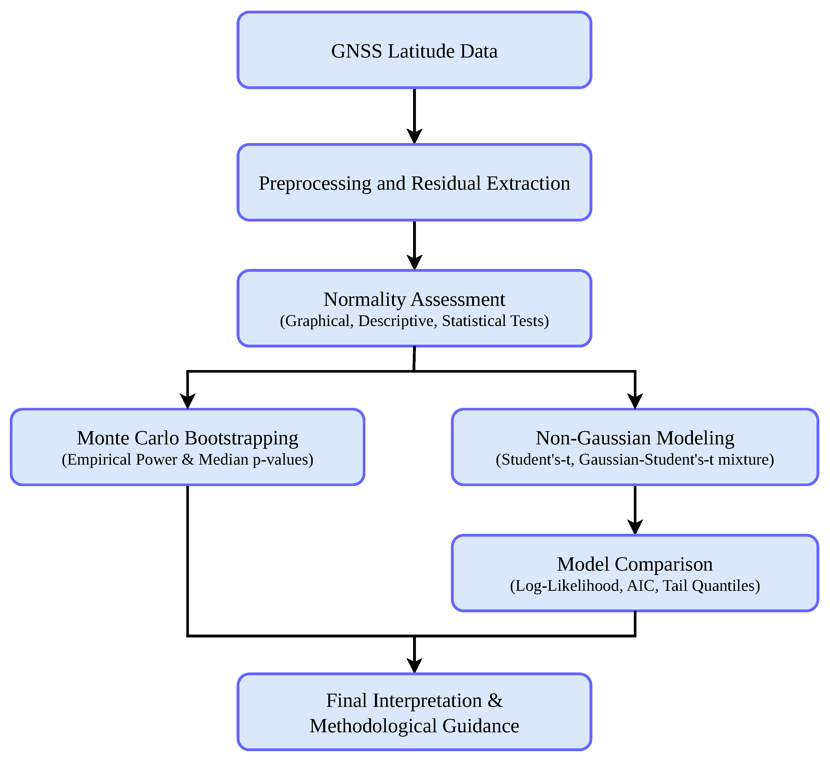
Figure 1 summarizes the complete analysis workflow, including normality assessment, test performance evaluation, and non-Gaussian error modeling.
3.1.1. Graphical Methods
Graphical tools provide an intuitive way to identify departures from normality [
8]. They do not provide formal statistical evidence but are widely used for preliminary assessment. A histogram shows the frequency of observations across defined intervals. A box plot summarizes data using five statistics: the minimum, lower quartile (
), median (
), upper quartile (
), and maximum. The whiskers extend from
and
to the most extreme non-outlier observations, indicating data spread beyond the central range. A normal Q–Q plot compares observed quantiles with those of a theoretical normal distribution; alignment along the reference line indicates a similar distributional shape. Although graphical methods provide valuable insight into distributional behavior, they are inherently qualitative and do not offer definitive evidence of normality [
33]. For this reason, graphical assessment is complemented by descriptive measures and formal statistical hypothesis tests.
3.1.2. Descriptive Statistical Measures
Descriptive statistics provide a concise way to summarize distributional properties, particularly asymmetry and tail behavior. In this study, skewness and kurtosis are used as indicators of deviations from normality. The fundamental concepts in this section are adapted from our previous work [
34].
Skewness
S measures the asymmetry of a probability distribution and is defined as
where
n is the sample size,
is the
ith observation,
is the sample mean, and
s is the sample standard deviation. A value of
corresponds to a symmetric distribution, whereas positive and negative values indicate right- and left-skewness, respectively [
35]. Skewness can also be approximated using Pearson’s second coefficient
where
denotes the sample median [
36].
Kurtosis
K describes tail heaviness and peak sharpness relative to the normal distribution and is defined as
The expression corresponds to excess kurtosis, so a normal distribution yields
. Values
indicate heavy tails and a sharper peak (leptokurtic behavior). Values
indicate lighter tails (platykurtic behavior) relative to the normal distribution [
37].
They may arise from measurement errors, unusual experimental conditions, or inherent variability in the underlying process. Outliers can distort statistical analyses and affect summary measures such as the mean and standard deviation, leading to misleading interpretations [
38]. In this study, outliers are detected using the
Z-score, defined as
The
Z-score expresses the distance between an observation and the sample mean in standard deviation units and is widely used for outlier detection. A
Z-score greater than 3 or less than
is commonly classified as an outlier under the assumption of normality [
39]. For non-Gaussian distributions, the
rule should be interpreted with caution because heavy tails, skewness, and other irregularities may increase the occurrence of extreme observations.
3.1.3. Statistical Hypothesis Testing
Statistical hypothesis testing for normality is broadly categorized into parametric and nonparametric methods. Parametric tests rely on assumptions such as independence, normality of residuals, homogeneity of variance, and interval or ratio-level measurements [
40]. In contrast, nonparametric tests relax these assumptions and are suitable for nominal or ordinal data. The present work examines seven widely used parametric normality tests, summarized in
Table 1 together with their formulae.
The assessment of normality is based on two complementary metrics: the test statistic and the corresponding p-value. The test statistic quantifies the deviation between empirical data and the assumed normal distribution. The p-value provides a probabilistic basis for hypothesis testing of .
To summarize results across repeated samples, the median
p-value is used as a robust indicator of central tendency. It is defined as
where
denotes the
p-value from the
ith repetition, with values ordered as
. As a robust measure of central tendency, the median reduces the influence of extreme
p-values and provides a stable summary of statistical evidence [
11]. In general,
p-values below a chosen significance level (e.g., 5%) lead to the rejection of
, indicating non-normality, whereas larger values indicate insufficient evidence against normality.
To quantify the performance of each test, the empirical power is defined as
where
is an indicator function that equals 1 if
and 0 otherwise. This metric estimates the probability of rejecting
and, under non-Gaussian conditions, reflects the ability of the test to detect deviations from normality [
37].
Median p-values and empirical power are jointly analyzed across varying sample sizes and significance levels. Evaluating both metrics provides a more complete assessment of test sensitivity and robustness under non-Gaussian GNSS conditions.
3.1.4. Heavy-Tailed Error Modeling
Given that GNSS measurements often exhibit non-Gaussian and heavy-tailed characteristics, this study also models GNSS latitude errors using flexible heavy-tailed distributions. The analysis focuses on latitude residuals as a representative one-dimensional case for investigating non-Gaussian behavior in GNSS positioning data. Recent studies indicate that GNSS measurement noise can deviate substantially from Gaussian assumptions under challenging conditions. It exhibits skewness, multimodality, and heavy-tailed behavior due to multipath, atmospheric disturbances, and signal obstruction [
26,
27,
30].
Student’s t Distribution
Student’s t distribution is a widely used heavy-tailed alternative to the Gaussian distribution that retains a unimodal and symmetric shape. In this study, the model is applied to GNSS latitude residuals to capture extreme deviations in one-dimensional positioning errors. Its probability density function is governed by location , scale , and degrees of freedom . Smaller values correspond to heavier tails and greater robustness to outliers.
Recent GNSS research shows that Student’s
t models improve robustness in measurement fusion and filtering under heavy-tailed noise and challenging environmental conditions [
27,
32]. The parameters
are estimated using maximum likelihood estimation (MLE). Numerical optimization uses a quasi-Newton method with positivity constraints on
and
. Student’s
t probability density function for a random variable
X with location
, scale
, and degrees of freedom
is given by:
where
denotes the Euler gamma function. As
decreases, the tails become heavier and extreme observations occur more frequently. Conversely, the distribution approaches the Gaussian model as
.
Gaussian–Student’s t Mixture Model
To represent both nominal and extreme error behavior, a two-component Gaussian–Student’s
t mixture model is employed. The choice is motivated by evidence that GNSS measurement noise may transition between approximately Gaussian and heavy-tailed regimes under varying observation conditions [
27]. The model is formulated using a latent binary variable
that assigns each observation
to one of two components. These are a Gaussian component with probability
w and a Student’s
t component with probability
. Within this framework, the Gaussian component represents nominal measurement noise under stable conditions, whereas Student’s
t component captures impulsive disturbances associated with environmental and propagation effects. Conditional on this unobserved label, the data follow
where
and
denote the mean and standard deviation of the Gaussian component, while
and
denote the location and scale of the Student’s
t component. Using the law of total probability, the marginal density of
is
where
and
denote the mixing probabilities of the Gaussian and Student’s
t components, respectively. Substituting Equation (
8) into Equation (
9) yields the mixture model representation
where
is the mixture weight that controls the relative contribution of the Gaussian component.
Model parameters are estimated using the expectation–maximization (EM) algorithm under a latent-variable formulation. In the E-step, posterior responsibilities are computed as , representing the probability that belongs to the Gaussian component. In the M-step, parameters are updated by maximizing the expected complete-data log-likelihood.
The mixture weight
w quantifies the proportion of observations associated with the Gaussian component. The term
represents the contribution of the heavy-tailed component. A larger Student’s
t contribution indicates stronger non-Gaussian behavior. A dominant Gaussian component suggests more stable measurement conditions. Together, the two components provide a flexible representation of the central distribution and the extreme deviations observed in GNSS measurements affected by environmental disturbances [
26,
29].
3.1.5. Model Evaluation and Comparison
To compare the non-Gaussian models with the Gaussian baseline, several complementary metrics are used to assess both overall fit and tail behavior. These metrics are particularly relevant for GNSS latitude error analysis, where heavy-tailed distributions and extreme deviations are common.
Log-Likelihood
The goodness-of-fit of a probabilistic model can be quantified using the log-likelihood
, which evaluates how well the model explains observed data. For a sample
and density
, it is defined as [
5]
where
denotes the model parameters. Larger values indicate a better fit to the empirical distribution. For Student’s
t distribution defined in Equation (
7) with parameters
, the log-density is
Substituting Equation (
12) into Equation (
11) yields the total log-likelihood expression
The same principle extends to the Gaussian–Student’s
t mixture model. For this model, with parameter vector
, the log-likelihood is obtained by substituting the mixture density from Equation (
10) into Equation (
11)
Tail Quantiles
Extreme positioning errors are particularly important in GNSS applications because they directly influence reliability and integrity monitoring. Their behavior is assessed using the 99% and 99.9% tail quantiles [
28,
42]. The
p-th quantile of a fitted distribution
is defined as
where
denotes the inverse cumulative distribution function. It gives the value
x such that
. Here,
. These quantiles assess how well models capture extreme-value behavior.
Root Mean Squared Error
Agreement between observations and model predictions is evaluated using Root Mean Squared Error (RMSE), a common accuracy metric [
4]. It is defined as
where
are observations, and
are model predictions. Smaller RMSE indicates closer agreement between the model and data. For Student’s
t model,
, yielding
For the Gaussian–Student’s
t mixture, the predicted value is
and substituting Equation (
19) into Equation (
17) yields
3.2. Experimental Setup and Data Acquisition
The measurement conditions were designed to reflect a harsh real-world environment. A low-cost GNSS receiver with the L76X GPS module was used in a stationary setup. The reference position was obtained from the Geoportal database [
43] and is
N and
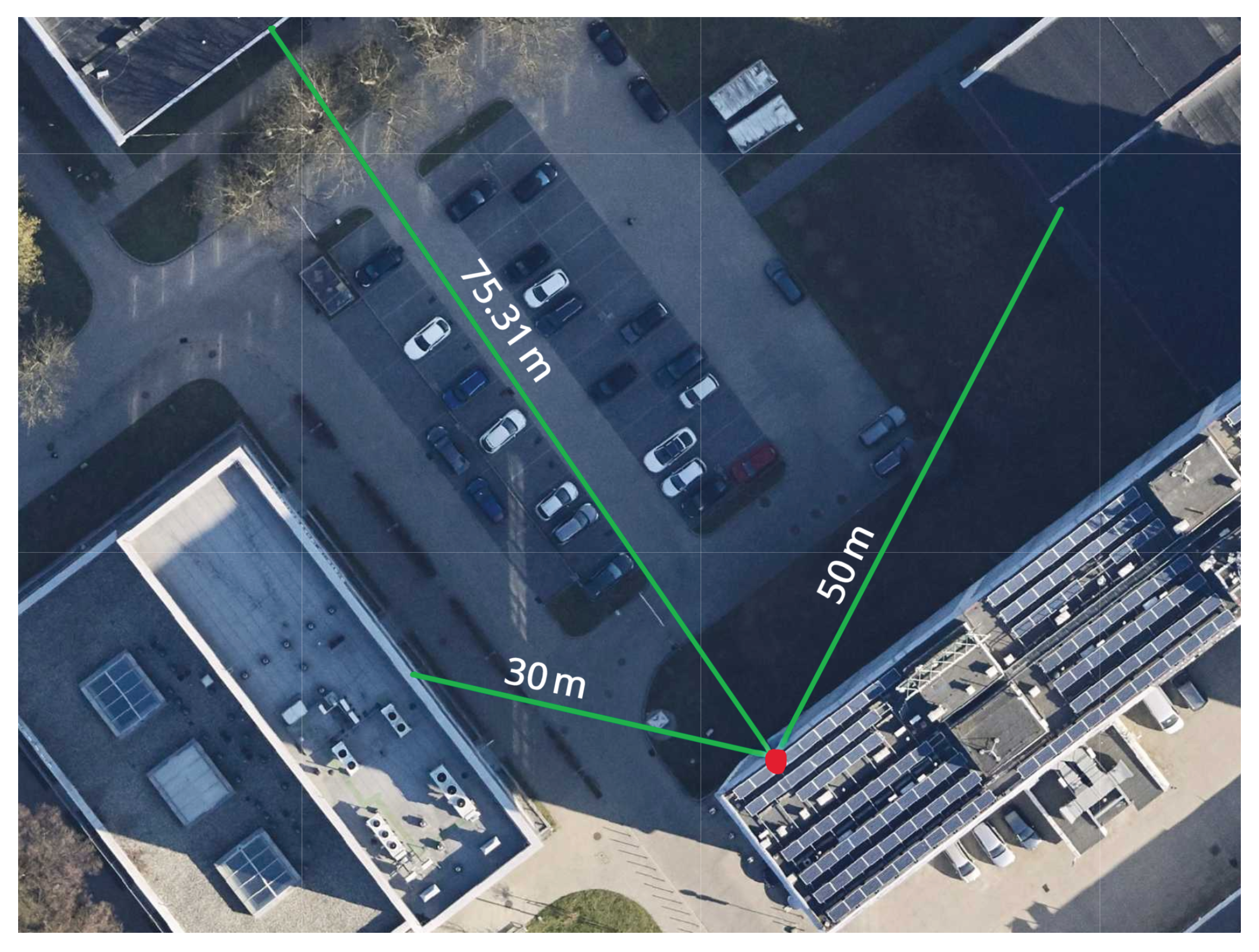
E. The receiver was placed on a windowsill in a typical urban environment with partial sky visibility (
Figure 2). The building height is approximately 30 m, and the receiver was located about 4.5 m above ground level. Surrounding structures block signals and introduce reflections, causing multipath, attenuation, and intermittent non-line-of-sight reception. This setup reflects practical GNSS use rather than optimized conditions. The aim is to represent typical environments rather than maximize positioning performance.
Real GNSS data were recorded continuously for a 48-h period at a 1 Hz sampling frequency, with an average of 12–15 tracked satellites. This resulted in 977,532 NMEA sentences. The observations include signals mainly from the GPS constellation, with temporal variations in the number of tracked satellites due to changes in visibility and satellite geometry. This long-duration dataset captures time-varying measurement conditions associated with these variations.
The stationary configuration minimizes motion-induced effects, allowing observed position variations to be attributed mainly to measurement uncertainties. However, GNSS errors remain influenced by time-varying environmental and propagation effects. Therefore, the setup provides a controlled framework for analyzing GNSS error statistics under quasi-static conditions rather than fully isolating intrinsic noise. The focus is not on optimizing measurement conditions, but on capturing representative GNSS error behavior in typical real-world environments.
From this dataset, 162,922 rows containing the $GPGGA message were extracted. These messages provide GNSS position solutions derived from real-time receiver processing. The study is based on these GNSS position solutions and reflects both measurement noise and geometric effects.
Latitude observations were used for statistical analysis as a representative one-dimensional case. A one-dimensional framework provides a clear and controlled setting for investigating distributional properties and normality test performance. It avoids multivariate dependence and serves as a basis for future two- and three-dimensional analyses. This approach makes latitude suitable for evaluating sensitivity to normality tests and heavy-tailed behavior under GNSS noise conditions.
In our previous work [
5], we analyzed covariance and correlation between latitude and longitude and evaluated two-dimensional horizontal positioning errors. Therefore, this study focuses on the one-dimensional latitude component to enable controlled distributional analysis. This simplification allows clearer assessment of distributional characteristics without multivariate dependence. Extending the framework to joint latitude–longitude modeling represents a natural continuation of this work.
All data processing and statistical analyses were carried out using standard numerical and statistical procedures in a reproducible Python 3.14-based environment. The methodology is independent of specific GNSS processing software because the primary objective is to evaluate statistical normality tests rather than positioning accuracy. The approach relies on standard GNSS receiver outputs, ensuring that results reflect typical measurement conditions while remaining reproducible across platforms. The workflow includes data preprocessing, descriptive statistics, normality testing, and Monte Carlo-based performance assessment, as summarized in
Figure 3.
After preprocessing, normality was evaluated using histograms, Q-Q plots, and several parametric normality tests. To assess the robustness of these tests under empirical GNSS error distributions, a Monte Carlo bootstrapping approach was used. Bootstrap samples were generated directly from the observed GNSS data, allowing statistical performance to be evaluated without assuming an underlying error distribution.
For each configuration, bootstrap samples were generated by resampling the 162,922 latitude observations with replacement. A total of 10,000 bootstrap replicates were generated for each sample size and significance level ( and ). For each test, p-values and rejection rates were aggregated. Median p-values and empirical power were then computed to quantify each test’s ability to detect deviations from normality.
4. Results
This section presents GNSS latitude error analysis. It covers outlier detection and graphical and statistical evaluation of normality. It also assesses test performance using Monte Carlo bootstrapping and compares non-Gaussian models for heavy-tailed behavior.
The considered GNSS latitude measurements are influenced by time-varying factors, including satellite constellation, atmospheric conditions, and receiver characteristics. Therefore, the observed behavior reflects GNSS errors under the specific experimental conditions of the dataset.
4.1. Data Outlier Detection
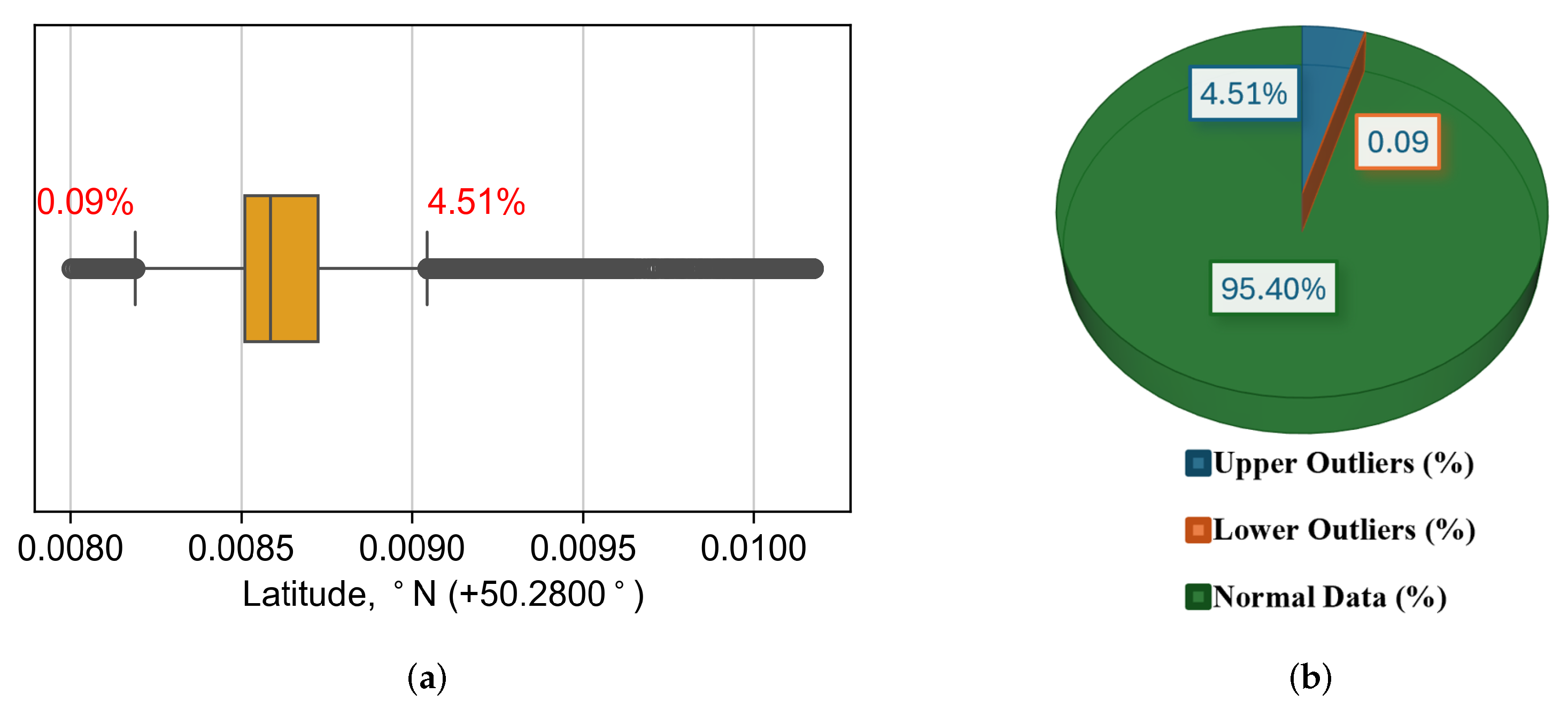
Figure 4a shows a box plot of the GNSS latitude data, and
Figure 4b presents the corresponding outlier distribution. The median lies slightly below the center of the interquartile range, indicating asymmetry. The lower (
) and upper (
) quartiles define a narrow central region of typical values. A substantial number of outliers appear beyond the upper whisker, while only a negligible fraction is observed below the lower whisker. This imbalance indicates a pronounced right-skewed behavior, with extreme values concentrated in the upper tail. Such asymmetry is consistent with GNSS measurement conditions influenced by the time-varying factors discussed earlier, which introduce large positioning errors [
6]. Quantitatively, upper outliers account for 4.51% of the dataset, whereas lower outliers are negligible.
4.2. Graphical Data Analysis
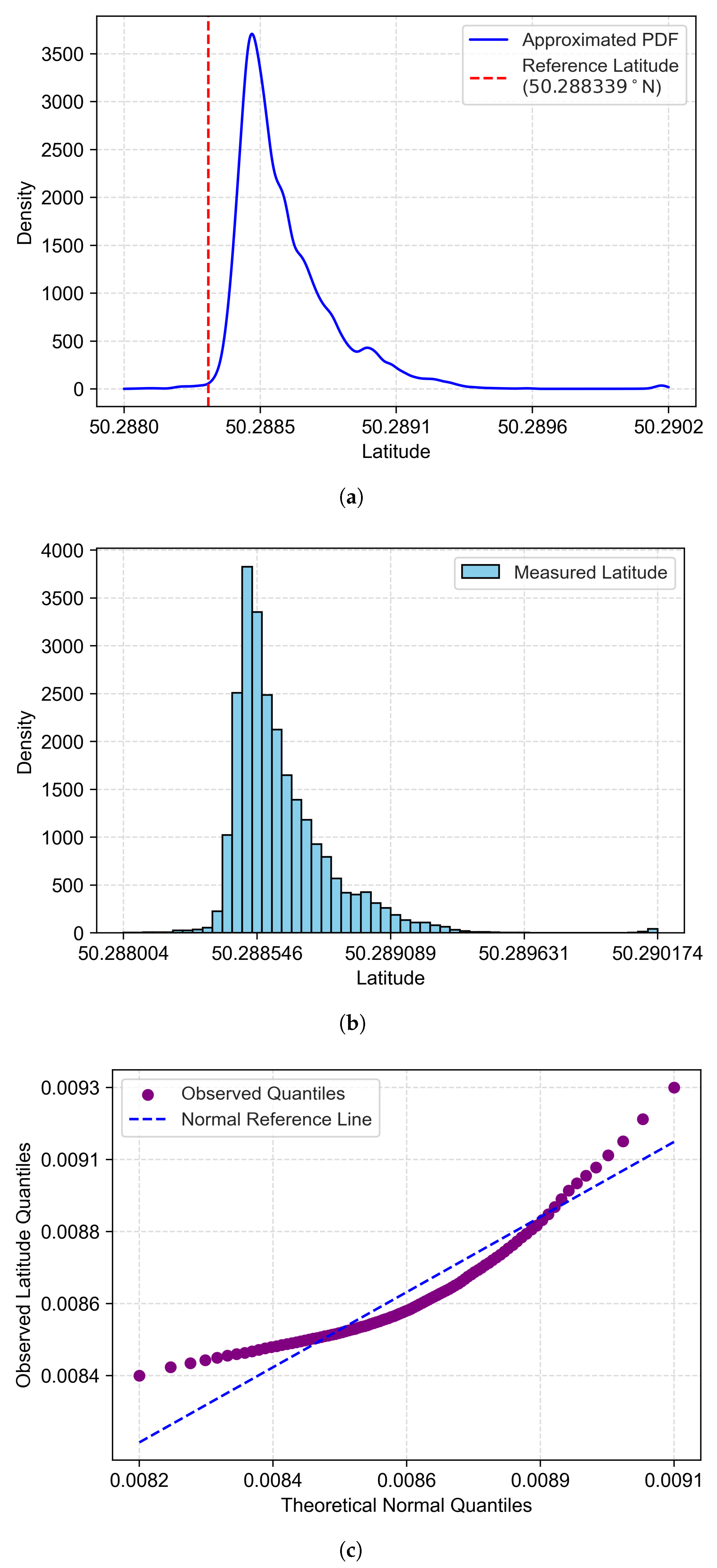
The GNSS latitude data show clear deviations from Gaussian behavior, characterized by positive skewness and a heavy-tailed distribution. The estimated probability density function confirms a peaked distribution with a long right tail, indicating leptokurtic behavior (
Figure 5a). The histogram deviates from the symmetric Gaussian curve, with increased probability mass in the upper tail (
Figure 5b). The Q–Q plot shows systematic divergence from the normal reference line, especially in the upper quantiles (
Figure 5c). These observations indicate strong departures from normality and pronounced right-skewness. The deviations are consistent with GNSS conditions affected by multipath, NLOS, and interference, producing asymmetric and heavy-tailed errors.
4.3. Descriptive Data Analysis (Skewness and Kurtosis)
A skewness value of
, computed using Equation (
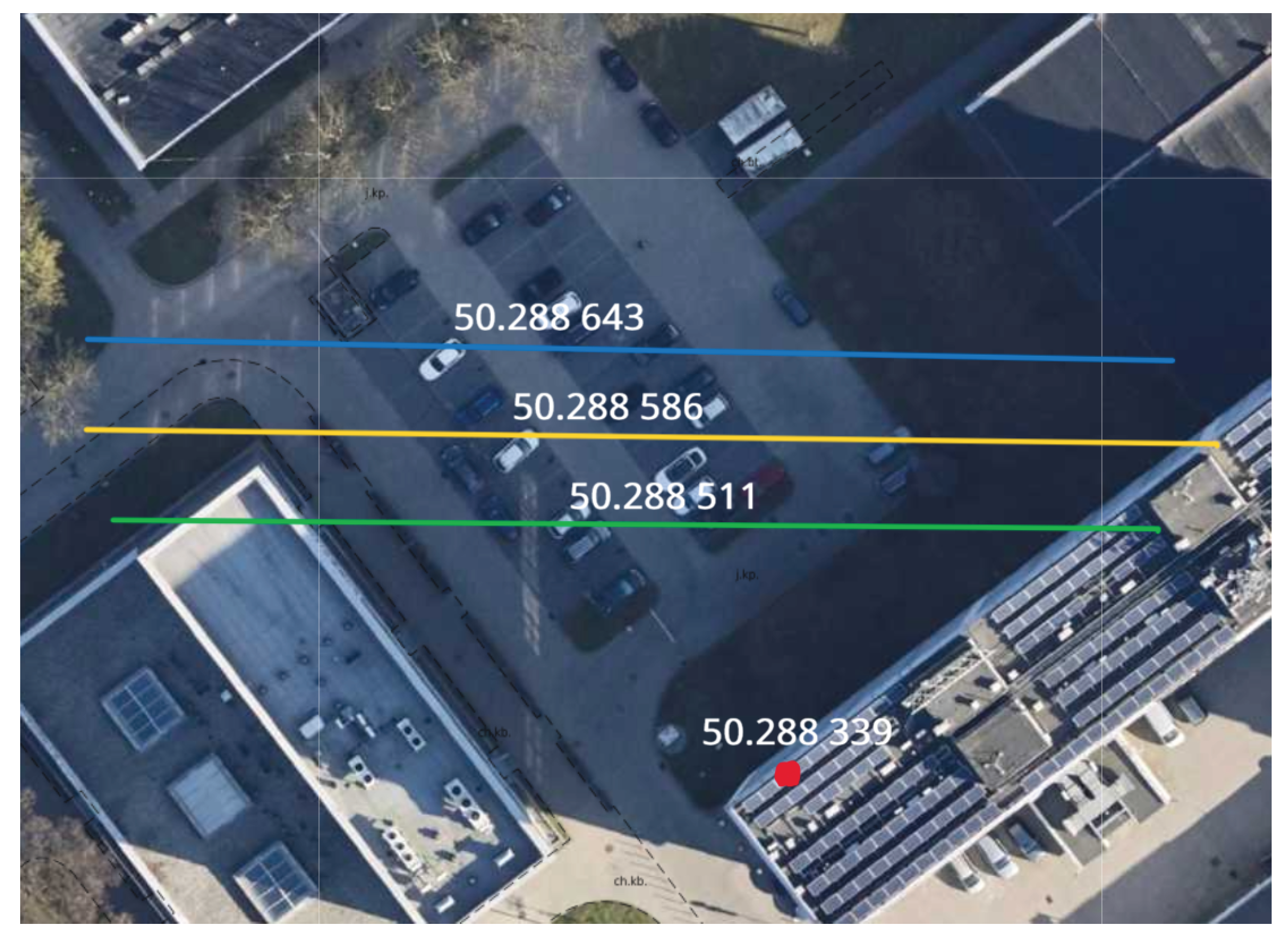
2), together with the fact that the mean exceeds the median, and the median exceeds the mode, confirms positive skewness. The mean, median, and mode are 50.288643°, 50.288586°, and 50.288511°, respectively (
Figure 6). This ordering characterizes a positively skewed distribution and indicates dominance of deviations above the Geoportal reference value 50.288339°N. The same pattern appears in
Figure 5, where the upper tail is substantially longer than the lower tail. This indicates that extreme positive deviations dominate the error distribution. This asymmetry is consistent with the observation environment, where the northern sky is relatively open, while the southern direction is fully blocked by the building. Consequently, lower-latitude observations occur less frequently.
4.4. Statistical Value of Tests
Test statistics for most tests, particularly AD, DA, JB, AJB, and CM, increase with sample size, indicating improved sensitivity to non-normality (
Table 2). Significant differences appear between small and large samples, especially for tests sensitive to higher-order moments such as skewness and kurtosis. The SW test shows strong sensitivity for small samples, whereas AD, DA, JB, and AJB become more effective as sample size increases, while LF shows comparatively low sensitivity.
These observations indicate that the detection capability of normality tests depends on both sample size and the underlying error structure. For GNSS data, this reflects time-varying factors such as satellite geometry, atmospheric effects, and receiver performance. High statistic values for AD, DA, JB, and AJB confirm strong deviations from Gaussian assumptions, consistent with heavy-tailed behavior in
Figure 5. The CM test shows a similar increasing trend with sample size in
Table 2.
4.5. Performance Evaluation of Normality Tests
The study evaluates the performance of AD, LF, SW, DA, JB, and AJB tests in empirical power and median p-value plots. The CM test is included only for computing statistical values. The evaluation uses GNSS latitude residuals as a one-dimensional case to assess test sensitivity under non-Gaussian behavior.
4.5.1. Comparison of Empirical Power for Latitude Data
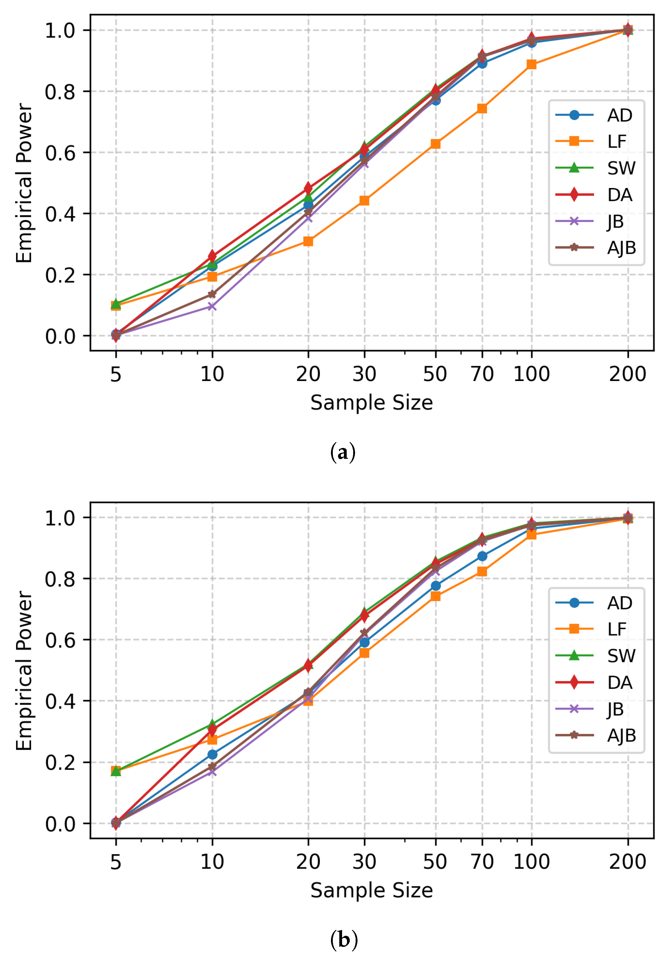
Empirical power increases with sample size for all tests (
Figure 7), with larger differences for small samples. The SW test dominates for
, while the DA test performs similarly for
. Both show strong sensitivity to non-normality under limited data.
At moderate sample sizes, the AD, JB, and AJB tests also achieve high power, whereas the LF test requires larger samples to reach similar performance. This trend highlights the dependence of test performance on sample size, especially for GNSS data where non-Gaussian features may require more observations.
Increasing the significance level from
to
improves the power of all tests, especially for small samples, as shown in
Figure 7b and
Table 3. The most notable improvement occurs for the SW test, followed by DA, JB, and AJB tests. Although AD and LF also improve, they remain less sensitive for smaller sample sizes
.
Higher significance levels increase sensitivity but also raise the risk of false rejection, indicating a trade-off between detection capability and false positives. Overall, empirical power increases with both sample size and significance level, demonstrating improved detection of non-normality under favorable conditions.
4.5.2. Comparison of the Median p-Value for Latitude Data
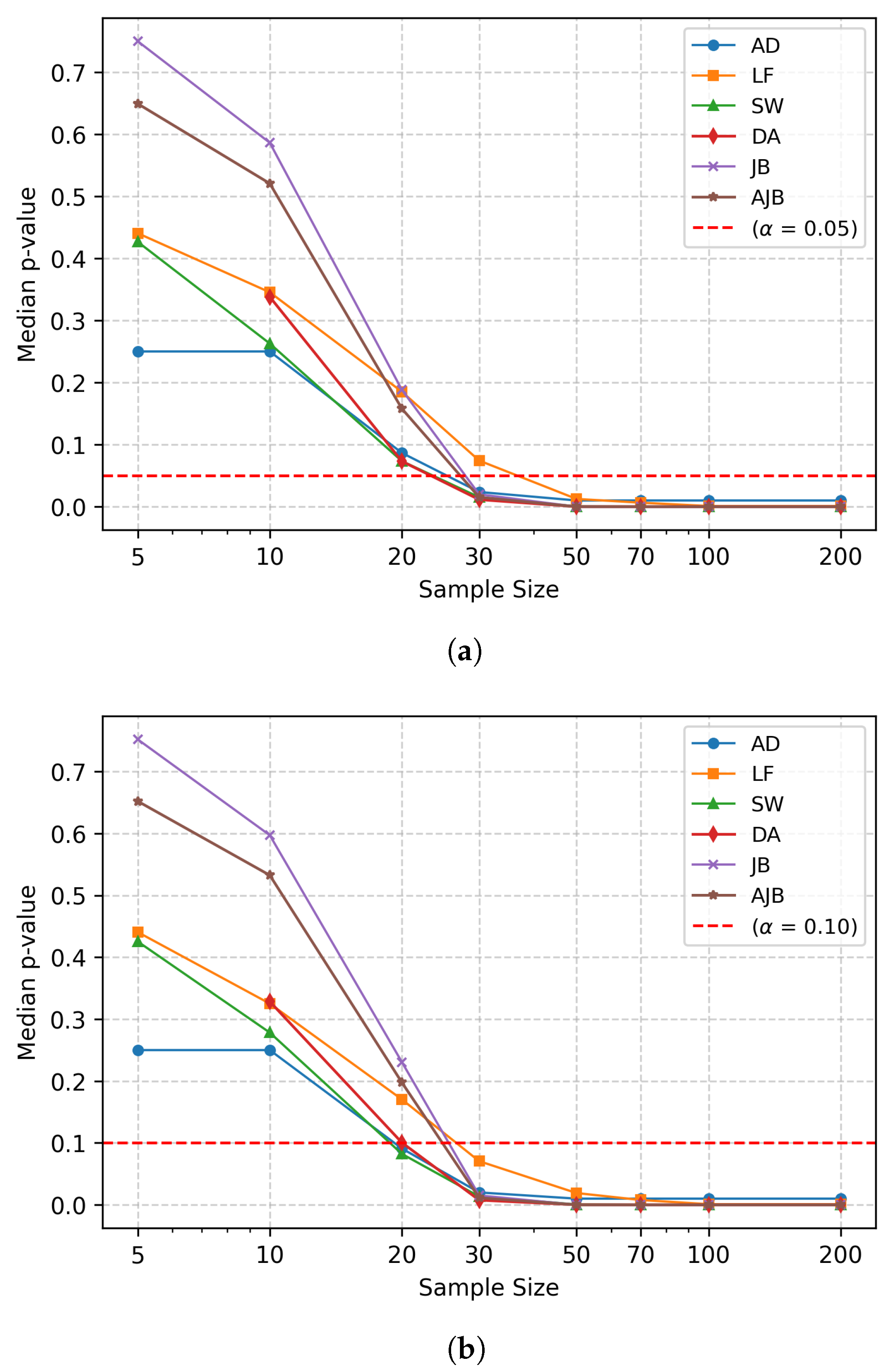
Median
p-values decrease with increasing sample size (
Figure 8), indicating improved detection of non-normality. For small samples
,
p-values often exceed 0.05 (
Table 4), so normality is not rejected despite clear deviations in
Figure 5.
This behavior reflects limited statistical power in small samples and may cause misclassification of GNSS errors as Gaussian. Increasing the significance level improves sensitivity but increases false positives. This trade-off highlights the importance of combining multiple tests and diagnostic methods when analyzing GNSS measurement distributions.
Overall, the results indicate a strong dependence of normality test performance on sample size and significance level. For small samples, most tests show low statistical power and often fail to reject normality. This occurs despite clear deviations observed in graphical diagnostics. This limitation highlights the risk of misinterpreting GNSS error distributions as Gaussian when sample sizes are insufficient.
4.6. Goodness-of-Fit Under Non-Gaussian Models
The data in
Table 5 show improved distributional fit as models transition from Gaussian to heavy-tailed and mixture representations. These models are fitted to GNSS latitude residuals to assess non-Gaussian behavior in a one-dimensional case study. The Gaussian model yields the lowest log-likelihood and overestimates moderate quantiles (e.g.,
). It also underrepresents extreme tail behavior compared to Student’s
t model at
. This inconsistency indicates that the Gaussian distribution does not capture the full range of deviations in the data.
Student’s t model improves the fit by accounting for heavy-tailed behavior related to impulsive errors. This leads to higher likelihood values and reduced estimates, indicating better representation of moderate deviations. However, the relatively large value suggests that a single heavy-tailed component cannot fully capture both nominal noise and rare extreme errors.
The Gaussian–Student’s t mixture model achieves the highest log-likelihood and lowest AIC, indicating the best overall fit. This model combines a narrow Gaussian core with a heavy-tailed Student’s t component that captures multipath and intermittent disturbances. Reduced and values show improved modeling of extreme positioning errors. This is important for GNSS reliability and integrity analysis. These observations agree with studies showing that mixture models outperform single-component approaches in challenging environments.
The Kolmogorov–Smirnov (KS) statistic measures the maximum absolute difference between empirical and theoretical cumulative distribution functions (CDFs) [
44,
45]. It provides a global measure of goodness-of-fit. Smaller KS values indicate better agreement between the model and observed data.
The goodness-of-fit metrics in
Table 6 show consistent improvement with heavier-tailed and mixture models. The Gaussian model has the highest KS, CM, AD, and RMSE values. This confirms a poor fit due to its inability to capture heavy-tailed behavior. Student’s
t model improves all metrics, especially AD, indicating better tail representation.
The Gaussian–Student’s t mixture model provides the best overall fit, with the lowest values across all metrics. It also shows a substantial reduction in CM and RMSE. This indicates that GNSS latitude errors are better described by a Gaussian core with a heavy-tailed component. This is consistent with measurement noise influenced by multipath and environmental disturbances.
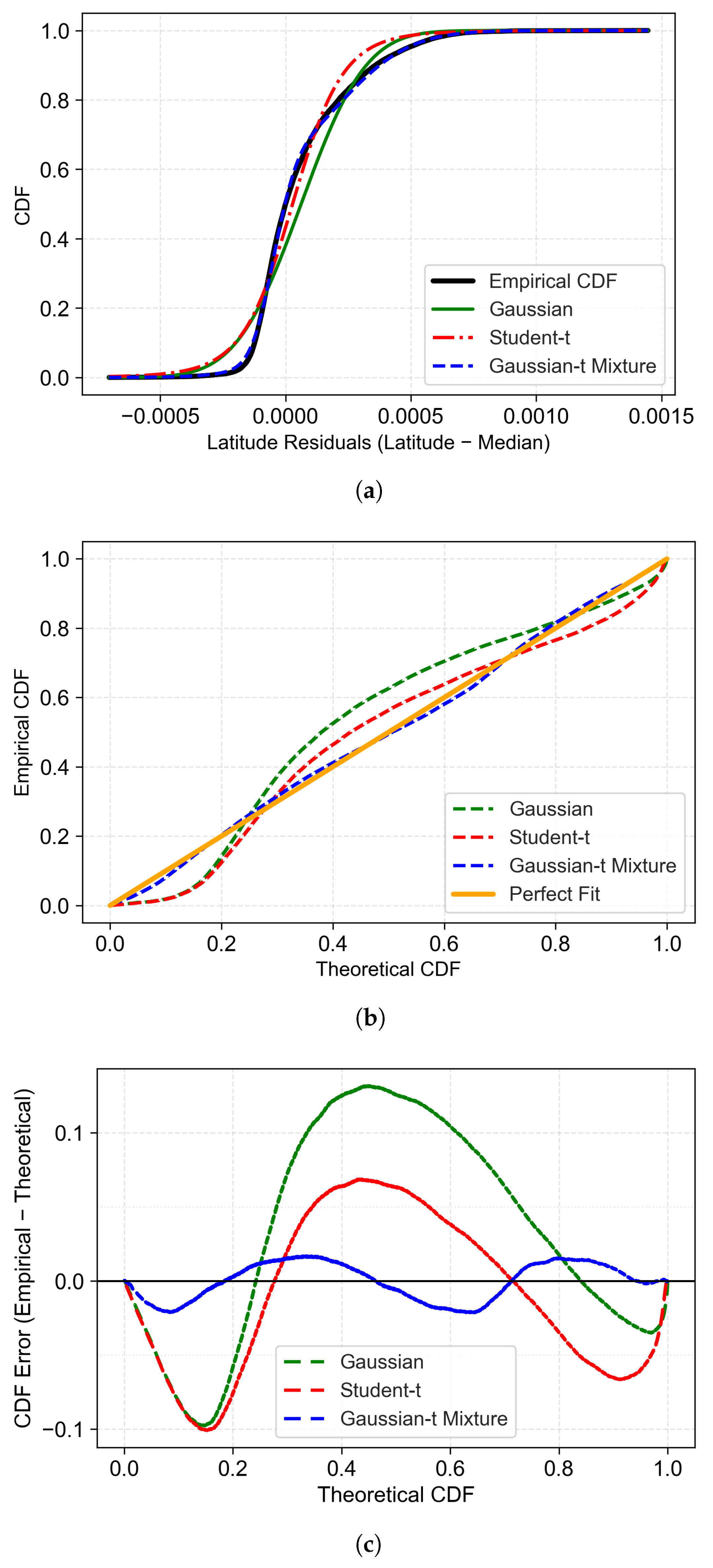
The goodness-of-fit diagnostics (
Figure 9) show that the Gaussian model provides the weakest fit to the GNSS residual distribution. Clear deviations appear in both the CDF and Q–Q plots. The largest discrepancies in the CDF error curves reach approximately
. Student’s
t model improves the fit by capturing heavy-tailed behavior. However, it still shows noticeable deviations.
In contrast, the Gaussian–Student’s t mixture model provides the closest agreement with the empirical distribution across all diagnostics. It shows near-linear alignment in the Q–Q plot and minimal errors, within approximately . GNSS latitude residuals exhibit non-Gaussian, heavy-tailed behavior. Flexible mixture models provide the most suitable representation of these characteristics.
The mixture weight provides insight into the relative contributions of nominal and impulsive GNSS errors. A higher Gaussian weight corresponds to more stable conditions dominated by receiver noise and favorable satellite geometry. In contrast, an increased Student’s t weight reflects the influence of multipath propagation, signal obstruction, or atmospheric disturbances. These effects introduce heavy-tailed deviations. Therefore, variations in mixture weights indicate changes in underlying GNSS error mechanisms under different environmental conditions.
5. Discussion
The presented results show that the performance of normality tests for GNSS latitude errors depends on sample size and error characteristics. For small samples, most tests have limited statistical power. This results in frequent non-rejection of the null hypothesis despite clear deviations observed in graphical diagnostics. This limitation introduces a critical risk in GNSS data analysis. It may lead to misinterpreting error distributions as Gaussian when the sample size is insufficient.
As sample size increases, all tests show improved sensitivity, allowing more consistent detection of non-Gaussian behavior. The SW and DA tests perform best for small and moderate samples. JB and adjusted AJB become more reliable for larger datasets. However, performance dependence on sample size shows that no single test is universally robust. This observation supports the use of a multi-test approach.
The behavior of median p-values further supports these observations. For small sample sizes, high p-values indicate only weak evidence against normality. This persists even when graphical diagnostics suggest clear departures. For larger samples, p-values decrease rapidly, indicating improved detection of deviations. Raising the significance level increases sensitivity but also elevates the risk of false rejection. This reflects a trade-off between detection capability and statistical reliability.
From a GNSS perspective, these findings relate to the measurement process. GNSS errors are affected by time-varying factors, including satellite geometry, atmospheric delays, multipath, and receiver limitations. These effects introduce nonstationarity and impulsive components not captured by Gaussian assumptions. They also vary across observation epochs. Accordingly, the study evaluates aggregate GNSS error behavior under varying conditions rather than assuming identical properties across epochs.
The goodness-of-fit diagnostics further support this interpretation. The Gaussian model provides the weakest representation of the GNSS latitude residual distribution. It shows significant deviations in both tails across the empirical CDF, Q–Q plots, and error metrics. These discrepancies indicate that Gaussian assumptions fail to capture both central tendency and extreme deviations.
In contrast, Student’s t model improves the fit by accounting for heavy-tailed behavior and reducing errors from impulsive deviations. The Gaussian–Student’s t mixture model provides the closest agreement with the empirical distribution. It shows strong alignment with the empirical CDF, improved adherence to the Q–Q reference line, and minimal residual errors. This indicates that the mixture model captures both Gaussian-like behavior and heavy-tailed extremes in GNSS error distributions.
The identification of non-Gaussian characteristics in GNSS latitude errors has important implications for data processing. Gaussian-based models tend to underestimate extreme deviations under heavy-tailed behavior. This may lead to overconfident uncertainty estimates. In contrast, heavy-tailed models, such as Student’s t and the Gaussian–Student’s t mixture, provide improved robustness. They account for impulsive disturbances caused by environmental interference.
Integrating non-Gaussian modeling into GNSS processing frameworks can improve reliability. It also provides a more realistic representation of positioning uncertainty. Such approaches are particularly relevant for applications requiring robust performance under challenging environmental conditions.
However, these findings should be interpreted within the context of the experimental setup. In this work, GNSS latitude data are obtained from a stationary, low-cost receiver based on NMEA outputs, which include uncorrected error sources. As a result, observed non-Gaussian characteristics may be amplified relative to high-precision frameworks such as PPP or RTK, where advanced corrections are applied. Previous studies evaluating ionospheric correction strategies show that positioning accuracy and residual statistics vary with the adopted correction model and processing framework [
46,
47].
Overall, pronounced non-Gaussian behavior appears under the analyzed conditions, although its general applicability remains limited. Behavior may change in higher-precision GNSS solutions or in dynamic scenarios, where different error sources dominate. At the same time, persistent heavy-tailed and asymmetric features point to clear limitations of Gaussian assumptions. These characteristics support the use of more flexible statistical models for GNSS error characterization.
6. Conclusions
This study examines long-duration GNSS latitude observations to assess departures from Gaussian assumptions and evaluate widely used normality tests. Graphical diagnostics, descriptive statistics, and seven parametric tests point to non-Gaussian behavior, with skewness, heavy tails, and outliers. Monte Carlo analysis indicates that Shapiro–Wilk (SW) and D’Agostino (DA) are most sensitive for small and moderate samples. Jarque–Bera (JB) and adjusted Jarque–Bera (AJB) become more reliable as sample size increases. The SW test dominates for , while DA behaves similarly for . Under limited data, both capture deviations effectively. JB and AJB improve more rapidly with increasing sample size than Lilliefors (LF) and Anderson–Darling (AD). The same tendency appears in both empirical power and median p-value metrics. No single test performs well across all cases, which supports combining several diagnostics in GNSS analysis.
Based on these findings, an empirical guideline for GNSS data analysis is proposed. For datasets with fewer than 50 samples, SW and DA provide superior detection of non-Gaussian behavior. JB and AJB offer complementary reliability for larger datasets. The combined use of multiple tests, including tail-sensitive and omnibus statistics, improves reliability in assessing distributional assumptions.
To further characterize these deviations, heavy-tailed models, including Student’s t and the Gaussian–Student’s t mixture, are fitted to GNSS latitude data. These models improve goodness-of-fit relative to the Gaussian baseline, particularly for extreme deviations. The mixture model achieves the best performance and indicates that GNSS latitude errors are better described by Gaussian noise with occasional heavy-tailed disturbances. These findings show that Gaussian models may underestimate uncertainty, whereas heavy-tailed models provide a more robust and realistic representation of GNSS errors.
The proposed framework integrates normality diagnostics with non-Gaussian modeling to support reliable GNSS uncertainty assessment. It provides practical guidance for selecting appropriate statistical models under realistic conditions. This approach improves robustness in statistical inference, positioning algorithms, and integrity monitoring.
The findings are based on observations from a stationary low-cost receiver in a partially obstructed urban environment using NMEA-derived positioning outputs. This setup reflects practical GNSS use and enables realistic error characterization. However, statistical properties may vary with receiver type, processing strategy, environment, and dynamic conditions. Focusing on the latitude component as a one-dimensional case study may also limit generality.
Future work will incorporate high-precision reference solutions such as PPP or RTK to compare uncorrected and corrected positioning outputs. This comparison will clarify how advanced correction strategies influence GNSS error distributions and their conformity to Gaussian assumptions. It will complement findings obtained from NMEA-based analysis. The framework will also be extended to dynamic receivers, multi-location datasets, and joint latitude–longitude modeling. These extensions will allow for the evaluation of temporal correlation, satellite geometry, and environmental variability effects on GNSS errors.
Author Contributions
Investigation, data collection and assembly, data analysis and interpretation, visualization, methodology, software, and writing of the original manuscript, A.B.; writing, review and editing, O.K. and J.W.; resources, conceptualization, validation, supervision, and project administration, J.W.; funding acquisition, A.B., O.K. and J.W. All authors have read and agreed to the published version of the manuscript.
Funding
This work was funded by the Polish Ministry of Science and Higher Education under Grant No. 02/050/BKM26/0058.
Data Availability Statement
The raw data supporting the conclusions of this article will be made available by the authors upon reasonable request.
Acknowledgments
Microsoft M365 Copilot (GPT-5 chat model) was used during manuscript preparation and revision to assist with language refinement, grammar, spelling, punctuation, sentence structure, formatting, and readability. All suggestions were critically reviewed, revised where necessary, and validated by the authors. Particular attention was given to improving readability and reducing repetitive or formulaic language. The authors take full responsibility for the final content of the manuscript.
Conflicts of Interest
The authors declare no conflicts of interest.
References
- Hoskin, T. Parametric and Nonparametric: Demystifying the Terms. Mayo Clin. Res. 2025, 5, 1–5. [Google Scholar]
- Ghasemi, A.; Zahediasl, S. Normality tests for statistical analysis: A guide for non-statisticians. Int. J. Endocrinol. Metab. 2012, 10, 486–489. [Google Scholar] [CrossRef] [Scilit] [PubMed]
- Chen, W.; Genton, M.G. Are You All Normal? It Depends! Int. Stat. Rev. 2023, 91, 114–139. [Google Scholar]
- Hasan, A.M.; Chen, Y.-J. Flexible Modeling of Multivariate Skewed and Heavy-Tailed Data via a Non-Central Skew-t Distribution: Application to Tumor Shape Data. arXiv 2025, arXiv:2507.10465. [Google Scholar]
- Bantu, A.; Wiora, J. Statistical characterisation of GNSS data for a stationary receiver using non-Gaussian distributions. Meas. Sci. Rev. 2025, 25, 6. [Google Scholar] [CrossRef] [Scilit]
- Bantu, A.; Wiora, J. Impact of non-Gaussian noise on position accuracy provided by Global Navigation Satellite Systems (GNSS). IEEE Access 2025, 13, 161750–161761. [Google Scholar] [CrossRef] [Scilit]
- Yasyukevich, Y.; Zhang, B.; Devanaboyina, V. Advances in GNSS positioning and GNSS remote sensing. Sensors 2024, 24, 1200. [Google Scholar] [CrossRef] [Scilit] [PubMed]
- Kanhere, A.V.; Gupta, S.; Shetty, A.; Gao, G. Improving GNSS positioning using neural-network-based corrections. NAVIGATION 2022, 69, navi.548. [Google Scholar] [CrossRef] [Scilit]
- Alghananim, M.S.; Ochieng, W.Y. A General Extreme-Value-Based Gaussian GNSS Measurement Error Distribution for Mission-Critical Applications. J. Navig. 2024, 77, 695–708. [Google Scholar] [CrossRef] [Scilit]
- O’Shaughnessy, E.; Detrinidad, E.; Soyer, P.; Lecler, A. An introductory guide to statistics for the radiologist. Diagn. Interv. Imaging 2024, 106, 49–52. [Google Scholar] [CrossRef] [Scilit] [PubMed]
- Habibzadeh, F. Data distribution: Normal or abnormal. J. Korean Med. Sci. 2024, 39, e35. [Google Scholar] [CrossRef] [Scilit] [PubMed]
- Tiberius, C.; Borre, K. Are GPS data normally distributed. In Geodesy Beyond 2000, Proceeding of the Challenges of the First Decade, IAG General Assembly Birmingham, 19–30 July 1999; Springer: Berlin/Heidelberg, Germany, 2000; (IAG, 2000); pp. 243–248. [Google Scholar]
- Torabi, H.; Montazeri, N.H.; Grané, A. A test for normality based on the empirical distribution function. SORT 2016, 40, 55–88. [Google Scholar] [CrossRef] [Scilit]
- Uhm, T.; Yi, S. A comparison of normality testing methods by empirical power and distribution of p-values. Commun. Stat.-Simul. Comput. 2023, 52, 4445–4458. [Google Scholar]
- Demir, S. Comparison of normality tests in terms of sample sizes under different skewness and kurtosis coefficients. Int. J. Assess. Tools Educ. 2022, 9, 397–409. [Google Scholar] [CrossRef] [Scilit]
- Khatun, N. Applications of normality test in statistical analysis. Open J. Stat. 2021, 11, 113–122. [Google Scholar] [CrossRef]
- D’Agostino, R.B. An Omnibus Test of Normality for Moderate and Large Size Samples. Biometrika 1971, 58, 341–348. [Google Scholar] [CrossRef]
- Patrício, M.; Ferreira, F.; Oliveiros, B.; Caramelo, F. Comparing the performance of normality tests with ROC analysis and confidence intervals. Commun. Stat.-Simul. Comput. 2017, 46, 7535–7551. [Google Scholar] [CrossRef] [Scilit]
- Yap, B.W.; Sim, C.H. Comparisons of various types of normality tests. J. Stat. Comput. Simul. 2011, 81, 2141–2155. [Google Scholar] [CrossRef] [Scilit]
- Pettitt, A. A Cramér–von Mises type goodness of fit statistic related to b1 and b2. J. R. Stat. Soc. B 1977, 39, 364–370. [Google Scholar] [CrossRef] [Scilit]
- Öztuna, D.; Elhan, A.H.; T üccar, E. Investigation of four different normality tests in terms of type 1 error rate and power under different distributions. Turk. J. Med. Sci. 2006, 36, 171–176. [Google Scholar]
- Thadewald, T.; Büning, H. Jarque–Bera test and its competitors for testing normality—A power comparison. J. Appl. Stat. 2007, 34, 87–105. [Google Scholar] [CrossRef] [Scilit]
- Knief, U.; Forstmeier, W. Violating the normality assumption may be the lesser of two evils. Behav. Res. Methods 2021, 53, 2576–2590. [Google Scholar] [CrossRef] [Scilit] [PubMed]
- Horváth, L.; Kokoszka, P.; Wang, S. Testing normality of data on a multivariate grid. J. Multivar. Anal. 2020, 179, 104640. [Google Scholar] [CrossRef] [Scilit]
- Castro, C.; Henriques, L.; Prata, F. Comparative Analysis of Normality Tests: Integrating Classical and Contemporary Approaches; Lecture Notes in Civil Engineering; Springer: Cham, Switzerland, 2024; Volume 494, pp. 356–365. [Google Scholar]
- Chen, J.; Zhang, W.; Feng, B.; Zhi, N.; Zhao, Y.; Lu, M. A Wasserstein Distance-Based Technique for the Evaluation of GNSS Error Characterization. GPS Solut. 2024, 28, 91. [Google Scholar] [CrossRef] [Scilit]
- Wu, J.; Jiang, J.; Tang, Y.; Liu, J. Gaussian–Student’s t Mixture Distribution-Based Robust Kalman Filter for GNSS/INS/Odometer Data Fusion. Remote Sens. 2024, 16, 4716. [Google Scholar] [CrossRef] [Scilit]
- Li, A.; Wang, Y.; Guo, M. Analysis of the Spatial Distribution and Common Mode Error Correlation in a Small-Scale GNSS Network. Sensors 2024, 24, 5731. [Google Scholar] [CrossRef] [Scilit] [PubMed]
- Barbero, T.; Matera, E.R.; Ekambi, B.; Chamard, J.; Abbia, M.E. Toward an Interpretable Multipath Error Model from GNSS Observables Through Deep Learning. Eng. Proc. 2026, 126, 14. [Google Scholar] [CrossRef] [Scilit]
- Li, Z.; Yan, P.; Wen, W.; Hsu, L.-T. Cauchy–Gaussian Overbound for Heavy-Tailed GNSS Measurement Errors. arXiv 2026, arXiv:2601.07299. [Google Scholar]
- Yan, P.; Song, B.; Xia, X.; Wen, W.; Hsu, L.-T. An Efficient Detector for Faulty GNSS Measurements under Non–Gaussian Noise Using Jackknife Statistics. arXiv 2025, arXiv:2507.03987. [Google Scholar]
- Qian, M.; Chen, W.; Sun, R. A Student’s t-Distribution-Based Filter Design for SINS/GNSS with Heavy-Tailed Noise. IET Electr. Power Appl. 2025, 19, e70076. [Google Scholar] [CrossRef] [Scilit]
- Koh, K.L.; Ahad, N.A. Normality for non-normal distributions. J. Sci. Math. Lett. 2020, 8, 51–60. [Google Scholar] [CrossRef] [Scilit]
- Bantu, A.; Kozyra, A.; Wiora, J. Normality tests for transformed large measured data: A comprehensive analysis. Stat. Transit. New Ser. 2025, 26, 195–208. [Google Scholar] [CrossRef] [Scilit]
- Tabachnick, B.G.; Fidell, L.S.; Ullman, J.B. Using Multivariate Statistics, 7th ed.; Pearson: Boston, MA, USA, 2019. [Google Scholar]
- Botev, Z.I.; Grotowski, J.F.; Kroese, D.P. Kernel density estimation via diffusion. Ann. Stat. 2010, 38, 2916–2957. [Google Scholar] [CrossRef] [Scilit]
- Joanes, D.N.; Gill, C.A. Comparing Measures of Sample Skewness and Kurtosis. Statistician 1998, 47, 183–189. [Google Scholar] [CrossRef] [Scilit]
- Mazarei, A.; Sousa, R.; Mendes-Moreira, J.; Molchanov, S.; Ferreira, H.M. Online boxplot-derived outlier detection. Int. J. Data Sci. Anal. 2025, 19, 83–97. [Google Scholar]
- Yaro, A.S.; Maly, F.; Prazak, P. Outlier detection in time-series received signal strength observation using z-score method with SN scale estimator for indoor localization. Appl. Sci. 2023, 13, 3900. [Google Scholar] [CrossRef] [Scilit]
- Lapko, A.V.; Lapko, V.A. Analysis of optimization methods for nonparametric estimation of probability density in large samples. Meas. Tech. 2024, 66, 839–847. [Google Scholar] [CrossRef] [Scilit]
- Linnet, K. Testing normality of transformed data. J. R. Stat. Soc. Ser. (Appl. Stat.) 1988, 37, 180–186. [Google Scholar] [CrossRef] [Scilit]
- Alghananim, M.S.; Ochieng, W.Y. Maximum Non-Bounded Difference (MnBD) Method for Overbounding GNSS Errors. GPS Solut. 2024, 29, 22. [Google Scholar] [CrossRef] [Scilit]
- Geoportal Poland. Geoportal Map Viewer. Geoportal Poland 2024. Available online: https://mapy.geoportal.gov.pl/imap/Imgp_2.html?}gpmap=gp0 (accessed on 9 June 2026).
- Drezner, Z.; Turel, O.; Zerom, D. A modified Kolmogorov–Smirnov test for normality. Commun. Stat. Simul. Comput. 2010, 39, 693–704. [Google Scholar] [CrossRef] [Scilit]
- Molin, P.; Abdi, H. New Table and Numerical Approximations for Kolmogorov–Smirnov/Lilliefors/van Soest Normality Test; Technical Report; University of Bourgogne: Dijon, France, 1998. [Google Scholar]
- Rovira-Garcia, A.; Ibáñez-Segura, D.; Orús-Perez, R.; Juan, J.M.; Sanz, J.; González-Casado, G. Assessing the quality of ionospheric models through GNSS positioning error: Methodology and results. GPS Solut. 2020, 24, 4. [Google Scholar] [CrossRef] [Scilit]
- Li, M.; Yuan, Y.; Zhang, T.; Xu, H.; Huo, X.; Zhang, W. Investigation of the Contribution of Five Broadcast Ionospheric Models (GPSK, NTCMG, NEQG, BDGIM, and BDSK) and IRTG to GNSS Positioning During Different Solar Activities in Solar Cycle 25. Space Weather 2024, 22, e2023SW003829. [Google Scholar] [CrossRef] [Scilit]
Figure 1.
Workflow of the proposed methodology for normality assessment and heavy-tailed GNSS error modeling.
Figure 1.
Workflow of the proposed methodology for normality assessment and heavy-tailed GNSS error modeling.
Figure 2.
Aerial view of the GNSS observation environment showing the spatial relationship between the receiver (red dot) and distances to nearby buildings. The base map is adapted from Geoportal Poland [
43].
Figure 2.
Aerial view of the GNSS observation environment showing the spatial relationship between the receiver (red dot) and distances to nearby buildings. The base map is adapted from Geoportal Poland [
43].
Figure 3.
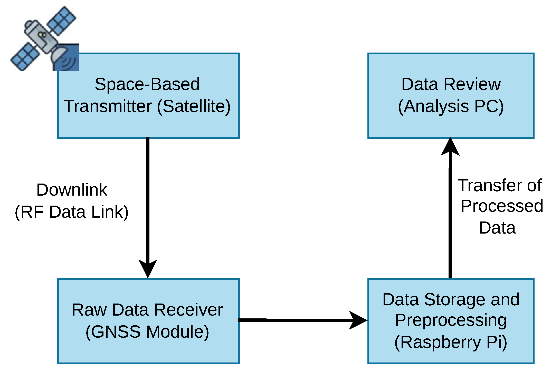
Experimental setup and GNSS data processing pipeline, illustrating the flow from data acquisition to analysis.
Figure 3.
Experimental setup and GNSS data processing pipeline, illustrating the flow from data acquisition to analysis.
Figure 4.
Distribution of outliers in GNSS latitude observations: (a) Box plot and (b) pie chart. For clarity, the latitude axis in (a) is referenced to the offset N, and only the least significant digits are shown.
Figure 4.
Distribution of outliers in GNSS latitude observations: (a) Box plot and (b) pie chart. For clarity, the latitude axis in (a) is referenced to the offset N, and only the least significant digits are shown.
Figure 5.
GNSS latitude distribution (degrees): (a) PDF via KDE, (b) latitude histogram, and (c) Q–Q plot. For clarity, the axes in (c) are referenced to an offset of N, with only the least significant digits shown.
Figure 5.
GNSS latitude distribution (degrees): (a) PDF via KDE, (b) latitude histogram, and (c) Q–Q plot. For clarity, the axes in (c) are referenced to an offset of N, with only the least significant digits shown.
Figure 6.
Spatial relationship between the receiver (red) and statistical measures of the GNSS latitude observations. The mode (green), median (yellow), and mean (blue) exhibit a progressive northward displacement relative to the Geoportal reference coordinate (50.288339°N). The base map is adapted from Geoportal Poland [
43].
Figure 6.
Spatial relationship between the receiver (red) and statistical measures of the GNSS latitude observations. The mode (green), median (yellow), and mean (blue) exhibit a progressive northward displacement relative to the Geoportal reference coordinate (50.288339°N). The base map is adapted from Geoportal Poland [
43].
Figure 7.
Empirical power for various normality tests across small and large sample sizes at significance levels (a) and (b) . Values are based on GNSS latitude data using 10,000 Monte Carlo simulations.
Figure 7.
Empirical power for various normality tests across small and large sample sizes at significance levels (a) and (b) . Values are based on GNSS latitude data using 10,000 Monte Carlo simulations.
Figure 8.
Median p-value for normality tests across small and large sample sizes at (a) and (b) . Values are obtained from GNSS latitude data using 10,000 bootstrap Monte Carlo simulations.
Figure 8.
Median p-value for normality tests across small and large sample sizes at (a) and (b) . Values are obtained from GNSS latitude data using 10,000 bootstrap Monte Carlo simulations.
Figure 9.
Goodness-of-fit diagnostics for fitted distributions: (a) Empirical versus theoretical CDFs, (b) Q–Q plot, and (c) CDF error curves for Gaussian, Student’s t, and Gaussian–Student’s t mixture models.
Figure 9.
Goodness-of-fit diagnostics for fitted distributions: (a) Empirical versus theoretical CDFs, (b) Q–Q plot, and (c) CDF error curves for Gaussian, Student’s t, and Gaussian–Student’s t mixture models.
Table 1.
Formulae for commonly used statistical normality tests.
Table 1.
Formulae for commonly used statistical normality tests.
| Test Name | Test Statistic | Ref. |
|---|
| Anderson–Darling (AD) | | [40] |
| Lilliefors (LF) | | [41] |
| Shapiro–Wilk (SW) | | [21] |
| D’Agostino (DA) | | [17] |
| Jarque–Bera (JB) | | [22] |
| Adjusted Jarque–Bera (AJB) | | [22] |
| Cramér–von Mises (CM) | | [20] |
Table 2.
Observed test statistic values for different normality tests at significance level .
Table 2.
Observed test statistic values for different normality tests at significance level .
| | Normality Tests |
|---|
| AD | LF | SW | DA | JB | AJB | CM |
|---|
| 5 | 0.339 | 0.257 | 0.896 | NaN | 0.622 | 0.934 | 1.67 |
| 10 | 0.500 | 0.221 | 0.885 | 2.53 | 1.24 | 1.51 | 3.33 |
| 20 | 0.858 | 0.192 | 0.880 | 5.77 | 3.92 | 4.33 | 6.67 |
| 30 | 1.24 | 0.181 | 0.876 | 9.42 | 8.10 | 8.66 | 10.0 |
| 100 | 3.92 | 0.154 | 0.871 | 31.0 | 49.4 | 50.4 | 33.3 |
| 200 | 7.54 | 0.144 | 0.860 | 69.1 | 162 | 164 | 66.7 |
Table 3.
Empirical power of normality tests at significance levels and .
Table 3.
Empirical power of normality tests at significance levels and .
| | | Normality Tests |
|---|
| | AD | LF | SW | DA | JB | AJB |
|---|
| 5 | 0.05 | 0.00 | 0.09 | 0.09 | 0.00 | 0.00 | 0.00 |
| | 0.10 | 0.00 | 0.16 | 0.17 | 0.00 | 0.00 | 0.00 |
| 10 | 0.05 | 0.22 | 0.17 | 0.24 | 0.25 | 0.13 | 0.11 |
| | 0.10 | 0.23 | 0.28 | 0.32 | 0.32 | 0.18 | 0.14 |
| 20 | 0.05 | 0.49 | 0.35 | 0.50 | 0.50 | 0.41 | 0.40 |
| | 0.10 | 0.43 | 0.41 | 0.52 | 0.52 | 0.43 | 0.41 |
| 30 | 0.05 | 0.58 | 0.44 | 0.61 | 0.60 | 0.57 | 0.56 |
| | 0.10 | 0.62 | 0.56 | 0.68 | 0.66 | 0.60 | 0.58 |
| 100 | 0.05 | 0.96 | 0.88 | 0.98 | 0.97 | 0.97 | 0.97 |
| | 0.10 | 0.96 | 0.94 | 0.99 | 0.99 | 0.99 | 0.99 |
| 200 | 0.05 | 1.00 | 1.00 | 1.00 | 1.00 | 1.00 | 1.00 |
| | 0.10 | 1.00 | 1.00 | 1.00 | 1.00 | 1.00 | 1.00 |
Table 4.
Median p-values for different normality tests at a significance level of .
Table 4.
Median p-values for different normality tests at a significance level of .
| | Normality Tests |
|---|
| AD | LF | SW | DA | JB | AJB |
|---|
| 5 | 0.25 | 0.38 | 0.38 | NaN | 0.73 | 0.62 |
| 10 | 0.19 | 0.20 | 0.15 | 0.28 | 0.54 | 0.43 |
| 20 | 0.02 | 0.06 | 0.01 | 0.06 | 0.14 | 0.11 |
| 30 | 0.01 | 0.02 | 0.00 | 0.09 | 0.02 | 0.01 |
| 100 | 0.01 | 0.00 | 0.00 | 0.00 | 0.00 | 0.00 |
| 200 | 0.01 | 0.00 | 0.00 | 0.00 | 0.00 | 0.00 |
Table 5.
Performance metrics for Gaussian, Student’s t, and Gaussian–Student’s t mixture models fitted to GNSS latitude data.
Table 5.
Performance metrics for Gaussian, Student’s t, and Gaussian–Student’s t mixture models fitted to GNSS latitude data.
| | Performance Metrics |
|---|
| Model | | | | |
|---|
| | () | () | () | () |
|---|
| Gaussian | 1.92 | −3.84 | 6.81 | 9.09 |
| Student’s t | 1.93 | −3.86 | 5.49 | 9.41 |
| Gaussian–Student’s t mixture | 1.97 | −3.94 | 5.35 | 6.90 |
Table 6.
Goodness-of-fit statistics for Gaussian, Student’s t, and Gaussian–Student’s t mixture models applied to GNSS latitude data.
Table 6.
Goodness-of-fit statistics for Gaussian, Student’s t, and Gaussian–Student’s t mixture models applied to GNSS latitude data.
| | Goodness-of-Fit Metrics |
|---|
| Model | KS | CM | AD | RMSE |
|---|
| Gaussian | 0.132 | 0.00612 | 958 | 0.0801 |
| Student’s t | 0.101 | 0.00324 | 680 | 0.0544 |
| Gaussian–Student’s t mixture | 0.0212 | 0.000325 | 308 | 0.0121 |
| Disclaimer/Publisher’s Note: The statements, opinions and data contained in all publications are solely those of the individual author(s) and contributor(s) and not of MDPI and/or the editor(s). MDPI and/or the editor(s) disclaim responsibility for any injury to people or property resulting from any ideas, methods, instructions or products referred to in the content. |