Task-Specific Negative Sample Selection for Multi-Hazard Susceptibility Mapping of Slope-Instability Hazards

Highlights

What are the main findings?

• A task-specific negative-sample selection method was proposed to reduce background mismatch in multi-hazard slope-instability susceptibility mapping.
• Task-specific negative samples improved the AUC and F1-score by 14.47% and 12.25% on average, respectively, compared with the other strategies.

What are the implications of the main findings?

• Negative-sample selection strongly affects both classification performance and study area-wide susceptibility-map quality.
• Hazard-specific adaptability in feature space is essential for balancing sample separability, boundary discrimination, and background representativeness.

Abstract

AI-based multi-hazard susceptibility mapping has become an important approach for identifying slope-instability hazards over large areas. However, in multi-hazard modeling, negative samples do not have a consistent stable meaning across hazard types: a background unit that is stable for one hazard may correspond to a potentially susceptible environment for another. Existing studies mainly focus on model optimization and accuracy improvement, but pay limited attention to task-level label confusion and background-sample mismatch caused by this issue. To address this gap, this study proposes a task-specific negative sample selection method based on the feature-space distribution of hazard-specific positive samples. Specifically, for each hazard type, the method uses its positive-sample centroid as a reference to rank the shared candidate background pool by feature-space distance. Rather than selecting only hard or easy negatives, it combines hard negatives closer to the centroid, easy negatives farther from it, and randomly supplemented background units to improve diversity. Taking the Minjiang River Basin in southeastern coastal China as the study area, the proposed method was compared with five benchmark strategies—random sampling, easy negative sampling, hard negative sampling, outside-buffer sampling, and buffer-ring sampling—using random forest (RF), boosted regression tree (BRT), multilayer perceptron (MLP), support vector machine (SVM), and logistic regression (LR). The results show that the dataset constructed using the proposed method improves the overall classification performance of the models, with average improvements of 14.47% and 12.25% in AUC and F1-score, respectively. The corresponding susceptibility maps also show the highest spatial screening efficiency, with the top 10% susceptible areas capturing 39.26% of historical hazard events, and only 27.06% of slope units were required to cover 80% of the hazards. In addition, this study further discusses the influence of hazard-specific adaptability on the feature-space distribution of negative samples, as well as the relationships among negative-sample selection strategies, classification performance, and study area-wide susceptibility-map quality. This study provides a new method for constructing reliable negative samples in regional multi-hazard susceptibility mapping of slope-instability hazards.

1. Introduction

Driven by climate change, urban expansion, land-use change, and other environmental disturbances, geohazards are increasing in both frequency and severity worldwide [1,2]. Among them, slope failures such as landslides, collapses, and debris flows are major sources of infrastructure damage and economic loss [3]. In mountainous regions, these hazards can coexist within the same topographic and hydrogeomorphic systems and exhibit spatially overlapping distributions due to shared regional-scale predisposing and triggering conditions [4,5]. Despite this spatial association, they differ in their movement processes and dominant environmental controls. Landslides involve the downslope displacement of soil or rock masses along a failure surface, whereas collapses entail the rapid detachment and falling of rock or soil from steep slopes [6]. By contrast, debris flows are characterized by the rapid channelized movement of water-laden sediment mixtures, and their development is strongly influenced by sediment supply, runoff conditions, and hillslope–channel connectivity [7,8]. Accurately identifying the susceptibility of these coexisting yet process-distinct hazards is therefore essential for regional risk screening and targeted disaster mitigation.

AI-based multi-hazard susceptibility mapping has become an increasingly important tool for geohazard prevention and mitigation [9,10,11]. By capturing nonlinear relationships between hazard occurrences and conditioning factors, machine learning techniques enable susceptibility modeling and spatial prediction across large areas [12]. For example, Cao et al. [4] constructed a multi-hazard inventory for Jiuzhaigou, China, using Google Earth interpretation and GIS, and generated susceptibility maps for collapses, landslides, and debris flows using RF, SVM, and XGBoost. Ullah et al. [13] developed a CNN-based multi-hazard susceptibility-mapping framework for the eastern Hindu Kush, Pakistan. Ye et al. [14] used ensemble machine learning models to map landslide and rockfall susceptibility in three hilly areas of southwestern China, namely Qijiang, Chishui, and Wuxi. Youssef et al. [15] applied BRT, GLM, RF, and other machine learning models to predict susceptibility to landslides, floods, and gully erosion in Saudi Arabia. Dai et al. [16] extended multi-hazard susceptibility assessment to Zhejiang Province, China, and revealed inter-hazard differences in spatial distribution and dominant conditioning-factor responses. Together, these studies highlight the value of machine learning in improving the accuracy and reliability of multi-hazard susceptibility mapping. However, existing multi-hazard studies have mainly focused on improving model performance. Comparatively less attention has been paid to training-dataset construction.

The effectiveness of susceptibility models depends not only on the data-driven algorithms used for modeling, but also on the quality of the susceptibility dataset [17,18,19]. This issue is particularly important in multi-hazard susceptibility mapping, where many existing studies still build separate single-hazard models and then integrate their outputs. As a result, the reliability of the final multi-hazard map largely depends on the quality of the training dataset constructed for each hazard type. Unlike positive samples, which are usually obtained from historical hazard inventories, negative samples are rarely observed as truly stable units. Instead, they are commonly constructed from background areas without recorded hazards according to predefined sampling rules [20,21].

Existing negative-sample construction methods mainly include random background sampling, buffer-constrained sampling, and environmental similarity-based selection [20,22]. Random background sampling treats units without recorded hazards as candidate stable samples, whereas buffer-constrained sampling excludes areas near known hazards or uses distance-stratified rules to improve spatial reliability and local environmental representativeness. These methods are simple and easy to implement, but they rely on the implicit assumption that unrecorded or distant areas can represent stable background conditions, which is not always valid in practice [23,24]. Environmental similarity-based methods further shift negative-sample selection from geographic space to feature space by comparing candidate background units with hazard samples in terms of topographic, geological, hydrological, and other environmental attributes [20,23,25,26]. However, these methods are commonly applied to individual hazard-specific susceptibility tasks and generally rely on a single sampling rule. In a multi-hazard context, the same candidate background unit may have different feature-space relationships with the positive samples of different hazards. A unified negative-sample selection rule may therefore be unable to accommodate task-specific differences in environmental conditions, boundary similarity, and sample discrimination difficulty.

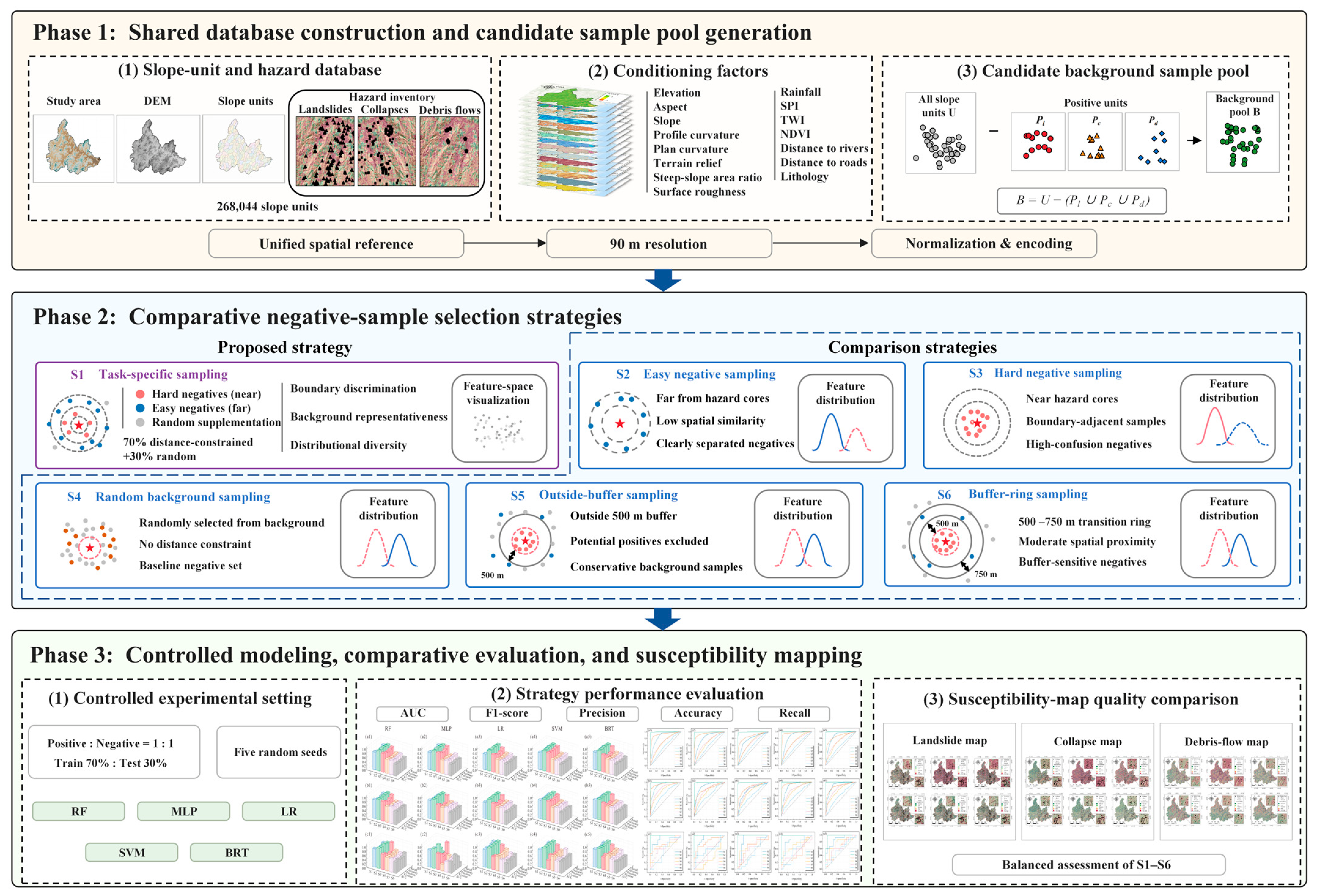
To address these issues, this study proposes a task-specific negative-sample selection method based on the feature-space distribution of positive samples for each hazard type (Figure 1). The method aims to construct negative-sample sets that better balance hazard-specific adaptability, boundary discrimination, and background representativeness in multi-hazard susceptibility mapping. Specifically, the positive-sample centroids of landslides, collapses, and debris flows are used as references to rank shared background samples by feature-space distance. Hard and easy negatives are then selected in a stratified manner and supplemented with randomly sampled background units to improve diversity, thereby producing negative samples tailored to the decision requirements of different hazards. Using the Minjiang River Basin as the study area, the proposed method is systematically compared with random background sampling, easy negative sampling, hard negative sampling, outside-buffer sampling, and buffer-ring sampling. Multiple machine learning models are further used to evaluate these strategies from two perspectives: classification performance and the spatial capture efficiency of study area-wide susceptibility maps [27,28]. The main contributions of this study are as follows:

Figure 1. Overall workflow of the paper.

(1) A task-specific negative-sample selection framework is proposed for multi-hazard susceptibility mapping of slope-instability hazards. Unlike conventional strategies that treat background units as a unified stable class, the proposed method constructs hazard-specific negative samples according to the feature-space distribution of positive samples for each hazard type.

(2) The study systematically evaluates how different negative-sample selection strategies affect both sample-level classification performance and study area-wide susceptibility-map quality. By comparing task-specific sampling with easy negative sampling, hard negative sampling, random background sampling, outside-buffer sampling, and buffer-ring sampling, this study reveals the inconsistency between high classification accuracy and reliable spatial hazard capture.

(3) Using landslides, collapses, and debris flows in the Minjiang River Basin as case studies, the proposed method is shown to improve the adaptability and stability of multi-hazard susceptibility mapping. The results demonstrate that task-specific negative samples can better balance sample separability, boundary discrimination, and background representativeness, thereby producing more reliable susceptibility maps across different hazard types.

2. Materials

2.1. Study Area

The Minjiang River is located in Fujian Province on the southeastern coast of China and is the largest river in the province. The basin covers approximately 5.99 × 10⁴ km², accounting for nearly half of the province’s land area [29]. The river system mainly consists of the Minjiang main stem and its major upstream tributaries, including the Jianxi, Shaxi, and Futunxi rivers, and drains southeastward into the East China Sea. The basin has a subtropical monsoon climate, with a mean annual temperature of approximately 17–19 °C and mean annual precipitation of approximately 1600–1700 mm. Precipitation is highly seasonal, with 70–80% of the annual total occurring during the flood season from April to September. This period can be further divided, according to the dominant weather systems, into Meiyu rainfall from April to June and typhoon-related rainfall from July to September [30]. Topographically, the basin generally descends from the Wuyi Mountains in the northwest toward the southeast. The upper basin is dominated by middle- and low-mountain terrain, deeply incised valleys, and steep channel gradients, whereas the middle and lower reaches gradually transition into hills and plains with widened, bead-like valley plains. The combination of mountainous–hilly terrain and concentrated heavy rainfall favors slope-runoff concentration, gully erosion, and slope instability.

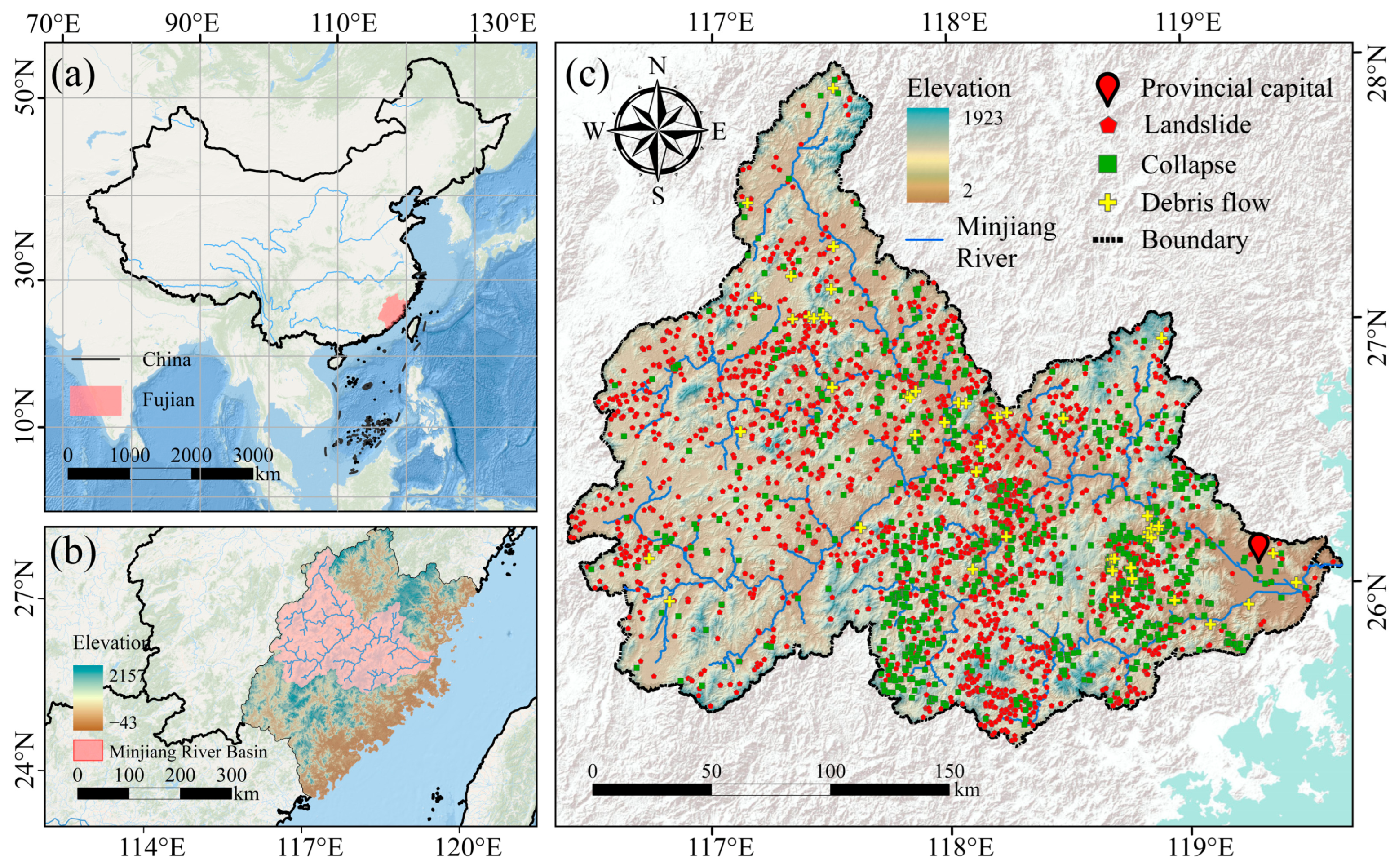
According to the Fujian Institute of Geological Survey, the Minjiang River Basin had recorded 3770 slope-instability hazard events as of December 2024, including landslides, collapses, and debris flows. Landslides were the most frequent, with 2685 events, whereas debris flows were the least frequent, with only 52 recorded events. Overall, slope-instability hazards in the Minjiang River Basin show marked differences among hazard types, with substantial variations in regional frequency and spatial occurrence conditions (Figure 2).

Figure 2. Geographical location and spatial distribution of landslides, collapses, and debris flows in the Minjiang River Basin. (a) Location of Fujian Province in China; (b) location of the Minjiang River Basin in Fujian Province; and (c) spatial distribution of the recorded landslides, collapses, and debris flows within the Minjiang River Basin. Different symbols and colors represent the three hazard types, as indicated in the legend.

2.2. Geohazard Conditioning Factors

Conditioning-factor selection directly affects the reliability of susceptibility models [31,32]. Because landslides, collapses, and debris flows share broadly similar environmental controls but differ in their occurrence mechanisms, their samples were constructed and compared within a unified environmental feature space. This unified factor system provides a common basis for comparing the three hazard tasks and for evaluating positive-sample distributions, background-sample similarity, and the suitability of negative samples for each task.

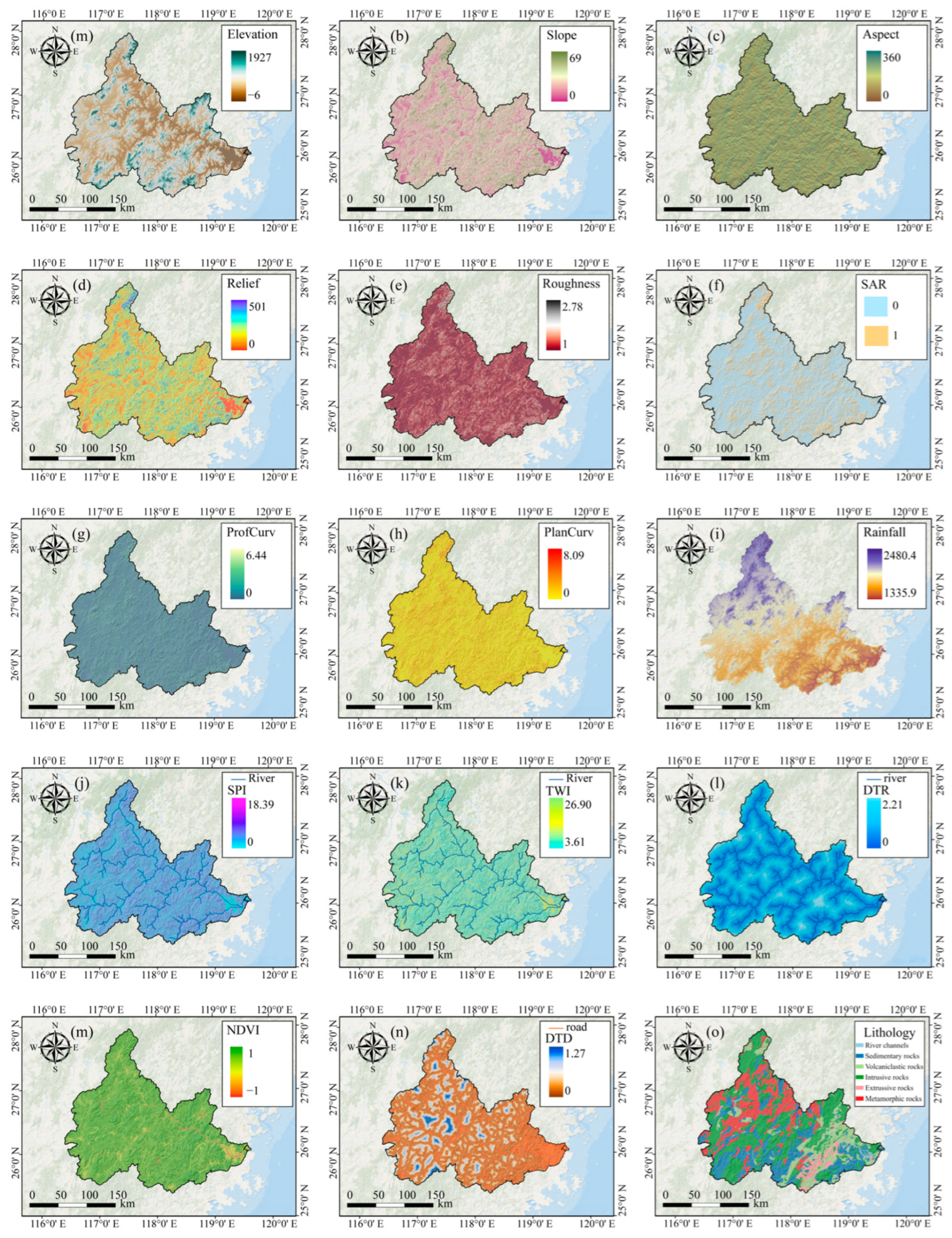
To comprehensively characterize the commonalities and specificities of the three hazards in terms of occurrence processes and environmental conditions, this study selected 15 commonly used susceptibility factors based on previous studies [33,34,35]. These factors represent terrain relief, slope morphology, hydrological convergence, geological conditions, vegetation cover, rainfall, and human activity. They include elevation, aspect, slope, profile curvature, plan curvature, terrain relief, steep-slope area ratio, surface roughness, rainfall, stream power index (SPI), topographic wetness index (TWI), normalized difference vegetation index (NDVI), distance to roads (DTDs), distance to rivers (DTRs), and lithology (Figure 3). Table 1 lists the main data sources and native spatial resolutions or map scales of the 15 hazard-related factors. To ensure consistency among spatial datasets from different sources, all conditioning factors were processed under a unified spatial reference and spatial resolution. All raster data were resampled to 90 m × 90 m and projected to the WGS 84/UTM zone 50N coordinate system.

Figure 3. Spatial distribution of the conditioning factors used for multi-hazard susceptibility modeling in the Minjiang River Basin: (a) elevation; (b) slope; (c) aspect; (d) relief; (e) roughness; (f) SAR; (g) ProfCurv; (h) PlanCurv; (i) rainfall; (j) river SPI; (k) river TWI; (l) river DTR; (m) NDVI; (n) road DTD; and (o) lithology.

Table 1. Conditioning factors used for multi-hazard susceptibility modeling, their data sources, and native spatial resolutions.

Factor	Description	Source	Native Spatial Resolution/Scale
Elevation (m)	Indicates regional topographic setting and controls variations in gravitational potential, temperature, moisture, and weathering environment.	Derived from DEM (https://www.gscloud.cn) using ArcGIS Pro 3.5.2	30 m × 30 m
Slope (°)	Describes the inclination of terrain and directly influences shear stress, runoff velocity, and the likelihood of slope failure.
Aspect	Represents slope orientation, which affects solar radiation, vegetation growth, soil moisture, and freeze–thaw or drying–wetting conditions.
Relief (m)	Measures local elevation variation and characterizes the intensity of terrain dissection and geomorphic energy.
Roughness	Describes the irregularity of the terrain surface and helps indicate local topographic fragmentation and erosion intensity.
Steep-slope area ratio (SAR)	Quantifies the proportion of steep terrain within each slope unit and represents the development degree of potentially unstable slope areas.
Profile curvature (ProfCurv)	Characterizes curvature along the downslope direction and influences runoff acceleration, erosion, and material transport.
Plan curvature (PlanCurv)	Characterizes curvature perpendicular to the slope direction and indicates flow convergence or divergence across the slope surface.
Stream power index (SPI)	Describes the potential erosive power of concentrated runoff and indicates areas prone to channel incision or slope toe erosion.
Topographic wetness index (TWI)	Estimates the tendency of water accumulation and indicates spatial differences in soil moisture and saturation potential.
Distance to rivers (DTR) (m)	Measures proximity to river channels and represents the potential influence of river incision, lateral erosion, and toe undercutting.
Rainfall (mm)	Represents the hydrological triggering condition by controlling infiltration, pore-water pressure variation, and surface runoff generation.	https://data.cma.cn/	1000 m × 1000 m
Normalized difference vegetation index (NDVI)	Indicates vegetation cover conditions, which are related to root reinforcement, interception, and surface erosion resistance.	Calculated from satellite imagery (https://www.gscloud.cn) using ArcGIS Pro 3.5.2	30 m × 30 m
Distance to road (DTD) (m)	Measures proximity to road networks and represents the possible effects of excavation, slope cutting, loading, and human disturbance.	Calculated from road vector (https://www.gisrs.cn/) using ArcGIS Pro 3.5.2	30 m × 30 m
Lithology	Describes the spatial variation in rock and soil types, which determines material strength, weathering resistance, and structural stability.	Geological Map of China, https://www.gisrs.cn/	1:2,500,000 scale (Raster data mapped to 30 m × 30 m based on ArcGIS pro 3.5.2)

3. Methods

3.1. Construction of Slope Units and Feature Extraction

A reasonable mapping unit is fundamental to susceptibility modeling of slope-instability hazards [36]. Compared with regular grid cells, slope units are typically delineated by natural topographic boundaries such as drainage divides and gully lines. They can therefore better preserve the geomorphic integrity of slopes and enhance both within-unit homogeneity and between-unit heterogeneity in topographic attributes [37,38,39]. Accordingly, this study used slope units as the basic spatial units for susceptibility modeling of landslides, collapses, and debris flows.

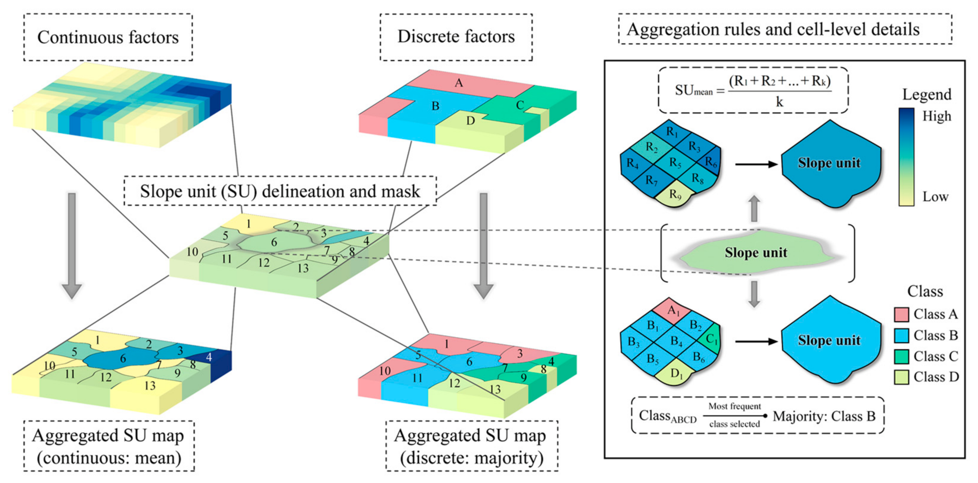
Slope units in the Minjiang River Basin were delineated using the r.slopeunits module proposed by Alvioli et al. [40]. After boundary correction and topological checking, a total of 268,044 slope units were obtained. Historical hazard points for landslides, collapses, and debris flows were then spatially overlaid with the slope units to identify positive units for each hazard type. The inventories were provided as point-based event records, with each point representing a documented event location rather than the full spatial extent of the event. The slope unit containing each point was therefore labeled as positive for the corresponding hazard type, and the resulting susceptibility was interpreted at the slope-unit scale. When multiple records of the same hazard type occurred within a single slope unit, only the occurrence attribute was retained to avoid double counting. Positive units of different hazard types were then used separately for the corresponding binary classification tasks. The numbers of slope units affected by landslides, collapses, and debris flows in the Minjiang River Basin were 2428, 928, and 51, respectively. Because different conditioning factors have different spatial representations, factor-specific rules were used to extract slope-unit attributes (Figure 4). For continuous factors, the mean pixel value within each slope unit was used to represent the overall environmental condition of that unit. For categorical factors, the category with the largest areal proportion within each slope unit was assigned as its dominant attribute.

Figure 4. Slope unit-based aggregation workflow for continuous and categorical conditioning factors.

3.2. Negative-Sample Selection Strategies

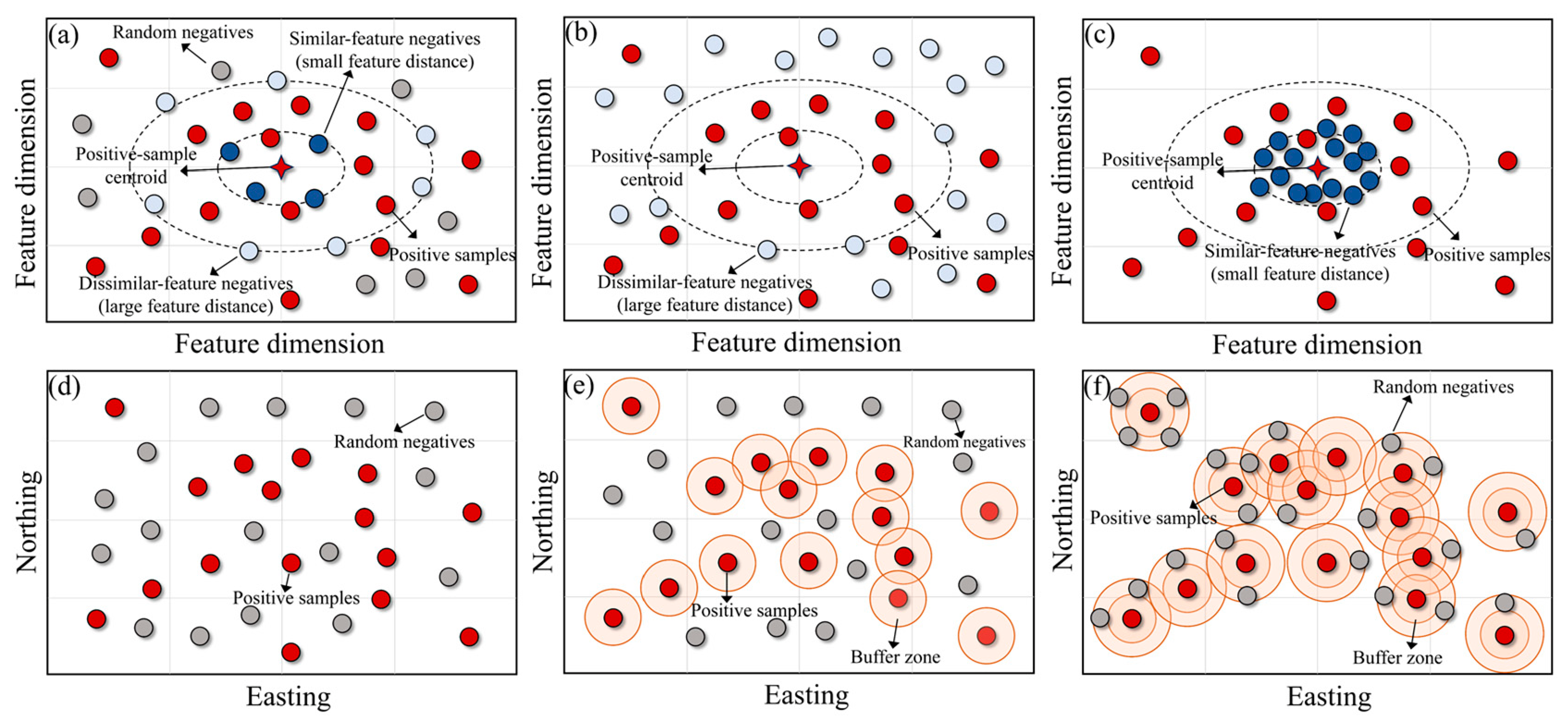
Figure 5 summarizes the proposed task-specific strategy and the five comparison strategies schemes adopted in this study from both feature-space and geographic-space perspectives. Specifically, feature space-based strategies select negative samples according to their distance from the positive-sample centroid, whereas spatially constrained strategies define candidate negatives using buffer zones around known positive samples. Based on this framework, the following subsections describe the construction of the candidate background pool and the implementation of each negative-sample selection strategy.

Figure 5. Illustration of negative-sample selection strategies in feature space and geographic space. (a) task-specific sampling (S1); (b) easy negative sampling (S2); (c) hard negative sampling (S3); (d) random background sampling (S4); (e) outside-buffer sampling (S5); and (f) buffer-ring sampling (S6). Colors indicate the sample categories shown in the legend, and dashed lines indicate distance or buffer constraints.

3.2.1. Candidate Background Sample Pool Construction

In susceptibility modeling of slope-instability hazards, positive samples can usually be identified directly by spatially overlaying historical hazard inventories with mapping units, whereas negative samples lack equally clear observational support [23]. Therefore, this study first constructed a candidate background sample pool as a common sampling source for different negative-sample selection strategies, rather than treating it as a set of truly stable units [18,20].

Let the set of all slope units in the study area be $U=\{u_1,u_2,\dots ,u_n\}$. For landslides, collapses, and debris flows, the corresponding sets of positive slope units are denoted as $P_l$, $P_c$, and $P_d$, respectively. $P_d$ To avoid misclassifying known unstable slope units as negative samples, all recorded positive slope units were removed from the full slope-unit set to construct a shared candidate background sample pool:

$$B=U-(P_l \cup P_c \cup P_d)$$

(1)

It should be emphasized that $B$ denotes only background units that were not recorded as slope-instability units in the historical hazard inventory. It does not imply that all units in $B$ are strictly stable. Therefore, all subsequent negative-sample selection strategies drew candidate samples from $B$, and hazard-specific negative samples were further screened using different sampling rules. For any hazard type h, if the number of positive samples is denoted as $\left|P_h\right|$, the same number of negative samples was selected from $B$. This produced a binary classification dataset with a positive-to-negative ratio of 1:1. This balanced setting was adopted to keep the sample size consistent across different negative-sample selection strategies and to facilitate a systematic comparison of how these strategies affect classification performance and susceptibility-map quality.

3.2.2. Task-Specific Negative-Sample Selection Strategy Based on Hazard-Specific Feature Space

In multi-hazard susceptibility mapping, different hazard types are usually modeled as separate binary classification tasks. Although recorded slope-instability units have been excluded from the candidate background pool, the meaning of a background unit as a negative sample still depends on the target hazard. A given background slope unit may have different feature-space distances and boundary relationships with the positive samples of landslides, collapses, and debris flows, and may therefore provide different information for different hazard models. Accordingly, negative-sample construction should not aim to identify a universally stable sample set. Instead, it should select and combine background samples that are better suited to hazard-specific discrimination and high-quality susceptibility mapping.

To this end, this study proposes a task-specific negative-sample selection method in hazard-specific feature space. For each target hazard, the positive-sample centroid is used as the reference, and shared candidate background samples are ranked according to their feature-space distance from this centroid. The ranked samples are then stratified and combined to include boundary-adjacent samples, typical background samples, and randomly supplemented samples. In this way, the proposed method constructs hazard-specific datasets that balance decision-boundary learning, background representativeness, and study area-wide mapping quality. For any hazard type $h$, the centroid of the positive samples is first calculated from its positive-sample set $P_h$:

$$c_h={\displaystyle \frac{1}{\left|P_h\right|}}{\displaystyle \sum _{u_i\in P_h}\varphi (x_i)}$$

(2)

where $x_i$ denotes the vector of conditioning factors for slope unit $u_i$, $\varphi (\cdot )$ denotes the standardized and encoded feature representation, and $c_h$ denotes the positive-sample centroid for hazard type $h$. The centroid is defined in the standardized environmental feature space rather than in geographic space. It represents the average environmental state of the recorded positive slope units for a given hazard type and is used to summarize the typical hazard-forming environmental conditions associated with that hazard. The feature-space distance between each candidate background unit in $B$ and the positive-sample centroid of hazard type $h$ was then calculated as follows:

$$d_h(u_j)={‖\varphi (x_j)-c_h‖}_2,u_j\in B$$

(3)

Here, $d_h(u_j)$ denotes the feature-space distance of candidate background slope unit $u_j$ relative to hazard type $h$ The L₂-norm was used to measure this feature-space distance because it provides a direct summary of the overall difference between standardized environmental feature vectors. This distance characterizes the similarity between a candidate background sample and the positive-sample distribution of the target hazard. A smaller distance indicates that the background sample is closer to the positive samples in feature space and therefore has stronger relevance for boundary discrimination. Conversely, a larger distance indicates greater separation from the positive-sample distribution and a higher likelihood of representing a typical background environment.

The candidate background sample pool $B$ was ranked according to $d_h(u_j)$. Samples close to the positive-sample centroid were treated as candidate hard negatives, representing boundary samples that are environmentally similar to the target hazard but have opposite labels. Samples far from the centroid were treated as candidate easy negatives, representing typical background samples that are clearly separated from the hazard samples. Rather than relying on either extreme alone, the proposed method combines distance-constrained screening with random supplementation to improve background coverage and distributional diversity in the negative-sample set.

For hazard type $h$, the number of negative samples was set equal to the number of positive samples; that is, $\left|N_h^{-}\right|=\left|P_h\right|$. The task-specific negative-sample set was composed of main negative samples and randomly supplemented negative samples:

$$N_h^{-} =N_h^{\mathrm{main}} \cup N_h^{\mathrm{rand}}$$

(4)

where $N_h^{main}$ represents the main negative samples selected from the candidate hard and easy intervals according to feature-space distance, and $N_h^{rand}$ represents the randomly supplemented negative samples drawn from the remaining candidate background pool. Let $\beta$ denote the random supplementation ratio; then:

$$\left|N_h^{\mathrm{rand}}\right|=\beta \left|N_h^{-}\right|$$

(5)

$$\left|N_h^{main}\right|=(1-\beta )\left|N_h^{-}\right|$$

(6)

In this study, $\beta$ was set to 0.3 based on preliminary parameter testing, which showed a relatively balanced performance between classification metrics and susceptibility-map quality. Detailed sensitivity results for different random supplementation ratios are provided in Tables S1 and S2 in the Supplementary Materials. Accordingly, 70% of the negative samples were obtained through distance-constrained screening, and 30% were randomly supplemented from the remaining candidate background pool. The distance-constrained component was further divided equally between the two ends of the hazard-specific distance ranking. Specifically, 35% of the negative samples were selected from the nearest candidate background units as hard negatives, and 35% were selected from the farthest candidate background units as easy negatives. Finally, the positive-sample set $P_h$ and the task-specific negative-sample set $N_h^{-}$ were combined to form the binary classification dataset for hazard type $h$:

$$D_h=P_h\cup N_h^{-}$$

(7)

Positive samples were labeled as 1, and negative samples were labeled as 0.

3.2.3. End-Member Negative-Sample Selection Strategies Based on Feature-Space Distance

End-member negative-sample selection strategies based on feature-space distance were used to examine how a single distance-screening logic affects model training and susceptibility mapping. Unlike the task-specific strategy, these strategies do not combine boundary-adjacent samples, distant background samples, and random supplementary samples. Instead, they select negative samples from the two extremes of the ranked feature-space distances, corresponding to hard and easy negatives. For hazard type $h$, the candidate background sample pool $B$ was ranked according to $d_h(u_j)$ in ascending and descending order as follows:

$$R_h^{\mathrm{desc}} =Sor{t}_{\mathrm{desc} }(B,d_h (u_j))$$

(8)

$$R_h^{\mathrm{asc}} =Sor{t}_{\mathrm{asc} }(B,d_h (u_j))$$

(9)

In these expressions, $R_h^{\mathrm{desc}}$ and $R_h^{\mathrm{asc}}$ denote the sequences of candidate background samples ranked by feature-space distance in descending and ascending order, respectively.

Under the easy negative-sample strategy, the first $\left|P_h\right|$ samples in $R_h^{\mathrm{desc}}$ were selected to form the easy negative-sample set $N_h^{\mathrm{easy}}$:

$$N_h^{\mathrm{easy}} =To{p}_{\left|P_h\right| }(R_h^{\mathrm{desc}})$$

(10)

These samples are far from the positive-sample centroid of the target hazard and therefore provide typical background information that is clearly differentiated from the hazard samples.

Correspondingly, under the hard negative-sample strategy, the first $\left|P_h\right|$ samples in $R_h^{\mathrm{asc}}$ were selected to form the hard negative-sample set $N_h^{\mathrm{hard}}$:

$$N_h^{\mathrm{hard}} =To{p}_{\left|P_h\right| }(R_h^{\mathrm{asc}})$$

(11)

where $N_h^{\mathrm{hard}}$ denotes the hard negative-sample set for hazard type $h$. These samples are close to the positive-sample centroid of the target hazard in feature space and therefore provide boundary-adjacent samples that are environmentally similar to the positive samples but have opposite labels.

Finally, the easy and hard negative-sample sets were separately combined with the corresponding positive-sample set to form two binary classification datasets:

$$D_h^{\mathrm{easy}} =P_h \cup N_h^{\mathrm{easy}}$$

(12)

$$D_h^{\mathrm{hard}} =P_h \cup N_h^{\mathrm{hard}}$$

(13)

3.2.4. Negative-Sample Selection Strategy Based on Random Background Sampling

Random background sampling is one of the most commonly used strategies for constructing negative samples in susceptibility mapping. It randomly selects samples from the candidate background pool without considering their feature similarity to the positive samples of the target hazard or their spatial distance from known hazard units. Therefore, it is often used as a baseline for evaluating other negative-sample selection strategies [25,41].

For any hazard type $h$, slope units equal in number to the positive samples were randomly drawn without replacement from the candidate background sample pool $B$ to construct the random negative-sample set $N_h^{\mathrm{rand}}$:

$$N_h^{\mathrm{rand}} =\mathrm{RandomSample}(B,\left|P_h\right|)$$

(14)

where $\mathrm{RandomSample}(\cdot )$ denotes random sampling without replacement. The random negative-sample set was then combined with the corresponding positive-sample set to form the binary classification dataset under the random background-sampling strategy:

$$D_h^{\mathrm{rand}}=P_h\cup N_h^{\mathrm{rand}}$$

(15)

3.2.5. Negative-Sample Selection Strategy Based on Buffer-Constrained Sampling

Buffer-constrained spatial sampling introduces spatial-distance restrictions into random background sampling. These methods still rely on random selection from candidate background slope units, but constrain the spatial locations of negative samples by setting distance thresholds relative to known hazard units. This helps reduce the likelihood that negative samples are drawn from areas close to known hazards. According to the spatial constraint used, the two most common buffer-based strategies are outside-buffer sampling and buffer-ring sampling [18,42].

For any hazard type $h$, the positive slope-unit set $P_h$ was used as the basis for buffer construction. Let $r$ denote the buffer distance; in this study, $r$ = 500 m. The corresponding buffer can be expressed as:

$${ℬ}_h(r)=\mathrm{Buffer}(P_h ,r)$$

(16)

Candidate background slope units located within this buffer were excluded from the negative-sample selection domain, yielding the outside-buffer candidate set:

$$B_h^{\mathrm{out}}=B-\{u_j\in B|u_j\cap {ℬ}_h(500)\ne \varnothing \}$$

(17)

Next, the same number of slope units as the positive samples were randomly drawn without replacement from $B_h^{\mathrm{out}}$ to form the outside-buffer negative-sample set:

$$N_h^{\mathrm{out}}=\mathrm{RandomSample}(B_h^{\mathrm{out}},\left|P_h\right|)$$

(18)

The basic assumption of this strategy is that areas close to known hazard units may have higher environmental similarity and greater label uncertainty; therefore, they should not be directly used as negative samples.

Under the buffer-ring sampling strategy, two buffer distances were further defined, with $r_1$ = 500 m and $r_2$ = 750 m. The annular zone between the two buffers was used as the candidate range for negative-sample selection. The corresponding buffer-ring area can be expressed as follows:

$${ℛ}_h(500,750)={ℬ}_h(750)-{ℬ}_h(500)$$

(19)

By spatially overlaying the candidate background sample pool $B$ with this buffer-ring area, the buffer-ring candidate set was obtained:

$$B_h^{\mathrm{ring}}=\{u_j \in B\mid u_j \cap {ℛ}_h (500,750)\ne \varnothing \}$$

(20)

The same number of slope units as the positive samples were then randomly drawn without replacement from $B_h^{\mathrm{ring}}$ to form the buffer-ring negative-sample set:

$$N_h^{\mathrm{ring}}=\mathrm{RandomSample}(B_h^{\mathrm{ring}},\left|P_h\right|)$$

(21)

Compared with outside-buffer sampling, buffer-ring sampling does not draw negative samples from all background areas distant from known hazards. Instead, it restricts sampling to a transitional belt at a specified distance from known hazard units. By excluding highly uncertain near-hazard areas while retaining local geomorphic similarity to hazard-prone environments, this strategy provides negative samples with more controlled spatial context.

3.3. Machine Learning-Based Susceptibility-Mapping Models

To avoid strategy evaluation being dependent on a single model, this study used five machine learning models with different learning mechanisms to assess the effects of negative-sample selection on multi-hazard slope-instability susceptibility modeling. These models covered ensemble learning, neural networks, linear probabilistic modeling, kernel-based classification, and tree-based boosting. For each negative-sample strategy, binary datasets were constructed separately for landslides, collapses, and debris flows, and all models were trained using the same conditioning-factor system to ensure comparability across sampling strategies.

3.3.1. Random Forest (RF)

Random forest (RF) is an ensemble tree-based method [43]. It constructs multiple decision trees using bootstrap sampling and aggregates their outputs to generate final prediction probabilities. Because randomness is introduced in both sample selection and feature selection, RF reduces the sensitivity of individual trees to training data perturbations and improves generalization performance [44]. In geoscience, ecology, and remote-sensing classification, RF is widely used to model nonlinear relationships, mixed variable types, and interactions among conditioning factors [45].

3.3.2. Multilayer Perceptron (MLP)

A multilayer perceptron (MLP) is a feedforward neural network model composed of an input layer, one or more hidden layers, and an output layer [46]. Through successive nonlinear transformations, MLP maps environmental factors into higher-level feature representations and learns complex nonlinear relationships between positive and negative samples [47]. Compared with linear models, MLP is better able to capture implicit interactions among conditioning factors.

3.3.3. Logistic Regression (LR)

Logistic regression (LR) is a probabilistic classification model that estimates the probability of a sample belonging to the target class from a linear combination of input factors [48]. As a generalized linear model, LR has limited ability to represent complex nonlinear relationships and higher-order interactions among variables. However, its simple structure, interpretability, and stable training make it a commonly used baseline model in machine learning classification tasks [49].

3.3.4. Support Vector Machine (SVM)

Support vector machine (SVM) discriminates samples by identifying an optimal classification boundary that maximizes the margin between classes [50]. For nonlinearly separable problems, SVM uses kernel functions to map the original features into a higher-dimensional space, thereby improving its ability to model complex decision boundaries. Because slope-instability hazards are often controlled by multiple environmental factors and the boundary between positive and negative samples may be complex, SVM is well suited to small-sample and moderate-dimensional settings.

3.3.5. Boosted Regression Tree (BRT)

Boosted regression trees (BRTs) are ensemble tree models based on boosting [51]. By sequentially combining multiple weak learners, BRT can model nonlinear relationships and interactions among variables more effectively than a single decision tree. It is therefore suitable for capturing complex hazard-susceptibility patterns under heterogeneous environmental conditions [52]. In this study, BRT was used as the representative boosted-tree model.

3.4. Evaluation Criteria

This study evaluated model performance from two perspectives: classification performance and study area-wide susceptibility-map quality. Classification performance was assessed using accuracy, precision, recall, F1-score (F1), and AUC. Susceptibility-map quality was evaluated using two types of indicators: the hazard capture rate within high-susceptibility zones and the area proportion required to achieve a fixed hazard capture rate. The classification metrics were used to evaluate sample-level discrimination on the held-out positive–negative test subsets, whereas the map-quality metrics were used to examine how the trained models ranked all slope units across the study area.

3.4.1. Criteria for Evaluating Classification Performance

For each hazard-specific binary classification task, model predictions were categorized as true positives (TPs), true negatives (TNs), false positives (FPs), and false negatives (FNs).

Accuracy measures the proportion of correctly classified samples and reflects the overall correctness of the model:

$$\mathrm{Accuracy}={\displaystyle \frac{\mathrm{TP}+\mathrm{TN}}{\mathrm{TP}+\mathrm{TN}+\mathrm{FP}+\mathrm{FN}}}$$

(22)

Precision measures the proportion of predicted hazard samples that are true hazard samples and reflects the reliability of positive predictions:

$$\mathrm{Precision}={\displaystyle \frac{\mathrm{TP}}{\mathrm{TP}+\mathrm{FP}}}$$

(23)

Recall measures the proportion of actual hazard samples that are correctly identified by the model and reflects the ability to detect historical hazard samples:

$$\mathrm{Recall}={\displaystyle \frac{\mathrm{TP}}{\mathrm{TP}+\mathrm{FN}}}$$

(24)

The F1-score is the harmonic mean of Precision and Recall and summarizes the balance between the reliability and completeness of positive-sample identification:

$$\mathrm{F}1={\displaystyle \frac{2\times \mathrm{Precision}\times \mathrm{Recall}}{\mathrm{Precision}+\mathrm{Recall}}}$$

(25)

AUC is the area under the receiver operating characteristic (ROC) curve and measures the model’s overall ability to distinguish positive from negative samples across classification thresholds. Unlike threshold-dependent metrics, AUC reflects the ranking ability of predicted probabilities; values closer to 1 indicate stronger discrimination between hazard and background samples.

3.4.2. Criteria for Evaluating Susceptibility-Map Quality

Beyond classification performance, the core objective of susceptibility mapping is to use model-output probabilities to rank all slope units across the study area and identify as many potential hazard units as possible within a limited spatial extent. To characterize differences among negative-sample selection strategies in study area-wide mapping, this study evaluated susceptibility-map quality in terms of both hazard capture and spatial screening efficiency [53,54].

For any hazard type $h$, predicted probabilities were first obtained for all slope units in the study area using the trained model. All slope units were then ranked in descending order of predicted probability, and the top $q$% of slope units were extracted as the high-susceptibility set, denoted as $A_{h,q}$. On this basis, the hazard capture rate $C_q$ for hazard type $h$ was calculated as follows:

$$C_q ={\displaystyle \frac{\left|A_q\cap P_h\right|}{\left|P_h\right|}}$$

(26)

To quantify the spatial screening efficiency of susceptibility maps, the minimum area proportion required to capture a given proportion of historical hazard units was further calculated. Let $R$ denote the target hazard capture rate. The corresponding minimum area proportion $A_R$ can be expressed as:

$$A_R=\min \left\{q\right|C_q\ge R\}$$

(27)

A lower $A_R$ indicates that the model can capture the target proportion of historical hazards within a smaller high-susceptibility area, and therefore has higher spatial screening efficiency.

3.5. Data Preprocessing and Model Parameter Settings

To ensure a consistent comparison across different negative-sample selection strategies, all sample data were uniformly preprocessed before model training, and all experiments were conducted under the same data-partitioning scheme, conditioning-factor system, and model-parameter settings. For landslides, collapses, and debris flows, each negative-sample strategy was used to construct a binary dataset with a positive-to-negative ratio of 1:1. Stratified sampling was then used to divide each hazard-specific dataset into training and test sets at a ratio of 7:3, thereby preserving the positive-to-negative class proportion in both subsets.

For feature preprocessing, different conditioning factors had different units and value ranges. Variables with larger numerical ranges could dominate model training and feature-distance calculation if used directly. Therefore, continuous factors were normalized to the range [0, 1] using Min–Max normalization to ensure comparability among factors in feature space. Categorical factors, such as lithology, were numerically encoded and likewise scaled to [0, 1]. After preprocessing, all slope units were represented as feature vectors on a unified scale, providing consistent inputs for subsequent negative-sample screening, model training, and study area-wide susceptibility prediction.

The hyperparameters of RF, BRT, MLP, SVM, and LR were optimized using grid search. Parameter optimization was performed only within the training set using five-fold stratified cross-validation. The test set was not involved in hyperparameter selection and was used only for final model performance evaluation. To ensure a fair comparison among the six negative-sample selection strategies, the same hyperparameter search space and cross-validation settings were used for all hazard types and all sampling strategies. Parameter selection was based on the mean AUC from the five-fold cross-validation. The optimal parameter settings are listed in Table 2.

Table 2. Hyperparameter settings of the five machine learning models.

Hazard Type	Model	Hyperparameter Set
Landslide	RF	n_estimators = 100, max_depth = 12, min_samples_leaf = 5, max_features = sqrt
	BRT	n_estimators = 80, learning_rate = 0.05, max_depth = 3, subsample = 0.8, min_samples_leaf = 5
	MLP	hidden_layer_sizes = (64, 32), activation = relu, alpha = 0.0005, learning_rate_init = 0.001, max_iter = 500
	SVM	C = 2, kernel = rbf, gamma = scale, probability = true
	LR	penalty = l2, C = 1.0, solver = lbfgs, max_iter = 1000
Collapse	RF	n_estimators = 100, max_depth = 8, min_samples_leaf = 4, max_features = sqrt
	BRT	n_estimators = 100, learning_rate = 0.05, max_depth = 3, subsample = 0.8, min_samples_leaf = 5
	MLP	hidden_layer_sizes = (32, 16), activation = relu, alpha = 0.005, learning_rate_init = 0.001, max_iter = 800
	SVM	C = 1.0, kernel = rbf, gamma = scale, probability = true
	LR	penalty = l2, C = 0.5, solver = lbfgs, max_iter = 1000
Debris flow	RF	n_estimators = 100, max_depth = 4, min_samples_leaf = 3, max_features = sqrt
	BRT	n_estimators = 50, learning_rate = 0.01, max_depth = 2, subsample = 0.7, min_samples_leaf = 3
	MLP	hidden_layer_sizes = (16, 8), activation = relu, alpha = 0.05, learning_rate_init = 0.001, max_iter = 1000
	SVM	C = 0.5, kernel = rbf, gamma = scale, probability = true
	LR	penalty = l2, C = 0.1, solver = lbfgs, max_iter = 1000

Considering that some negative-sample selection strategies involve random sampling, sample construction and model training were repeated using five random seeds. The overall performance of each strategy was evaluated based on the repeated experiments. For visualizations, including susceptibility maps and sample distributions, one representative random seed was selected for display. This seed was not chosen according to the best performance, but rather as the run whose performance was closest to the mean performance of the corresponding strategy. This ensured that the visual results reflected the general characteristics of that strategy.

4. Results and Analysis

4.1. Differences in Feature-Space Distributions Among Negative-Sample Strategies

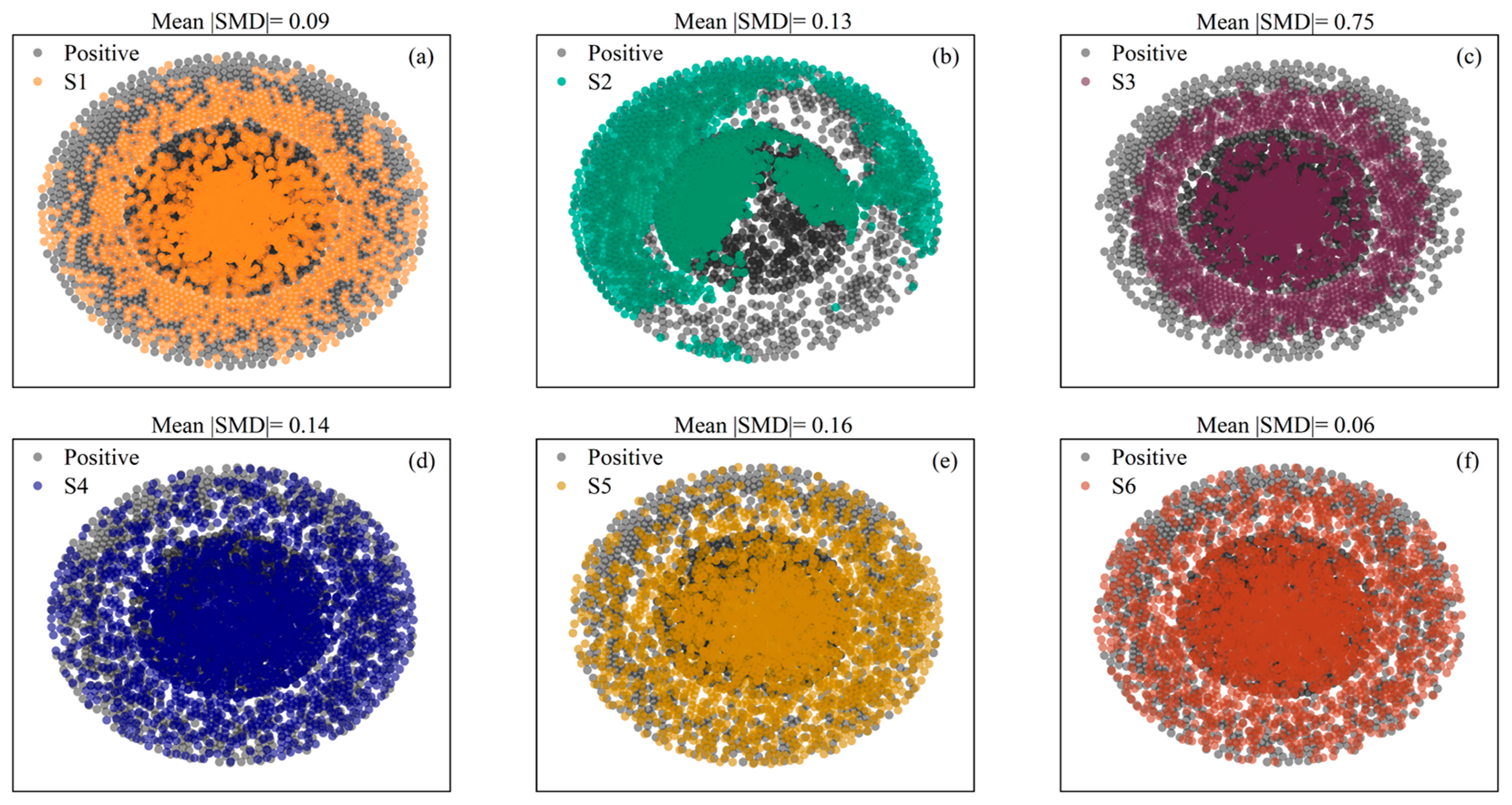
To analyze how different negative-sample selection strategies affected sample feature-space structure, t-SNE was used to project the feature matrices of the three hazard types into two-dimensional space. Figure 6, Figure 7 and Figure 8 show the distributions of positive samples for the landslide, collapse, and debris-flow tasks, together with the negative samples generated by the six strategies: task-specific sampling (S1), easy negative sampling (S2), hard negative sampling (S3), random background sampling (S4), outside-buffer sampling (S5), and buffer-ring sampling (S6). The corresponding feature-separation metric, Mean ∣SMD∣, is also shown. This metric represents the mean absolute standardized mean difference between negative and positive samples across all conditioning factors. Larger values indicate stronger overall feature separation between positive and negative samples, whereas smaller values indicate more similar feature distributions.

Figure 6. The t-SNE visualization results of positive and negative samples under six negative-sample selection strategies for landslide susceptibility modeling: (a) S1; (b) S2; (c) S3; (d) S4; (e) S5; and (f) S6.

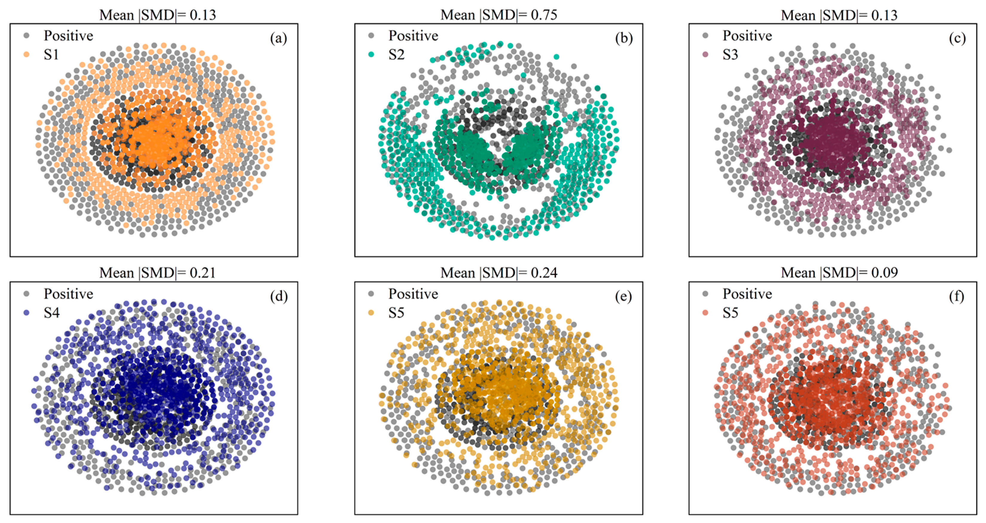
Figure 7. The t-SNE visualization results of positive and negative samples under six negative-sample selection strategies for collapse susceptibility modeling: (a) S1; (b) S2; (c) S3; (d) S4; (e) S5; and (f) S6.

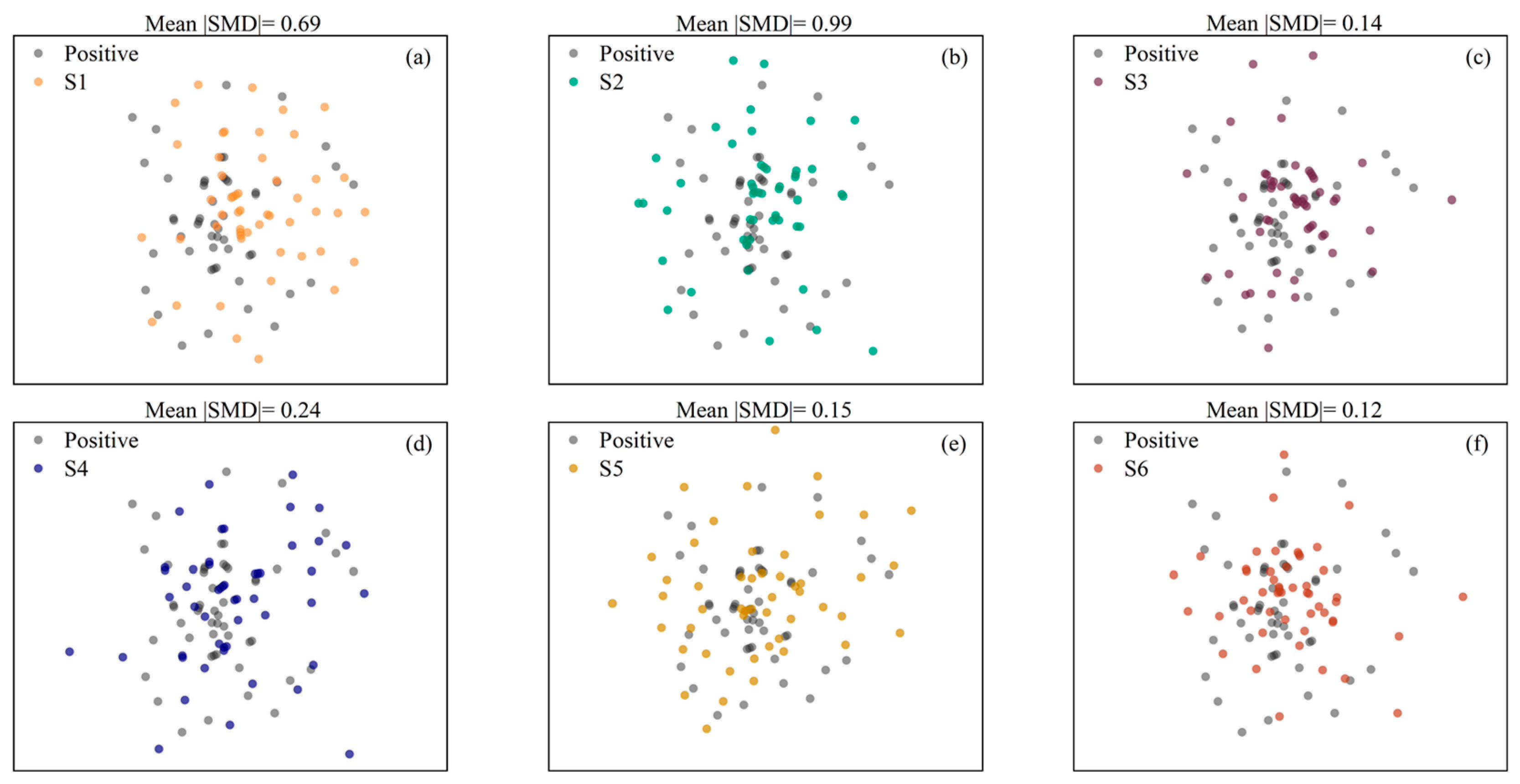
Figure 8. The t-SNE visualization results of positive and negative samples under six negative-sample selection strategies for debris-flow susceptibility modeling: (a) S1; (b) S2; (c) S3; (d) S4; (e) S5; and (f) S6.

Among the six strategies, S2 showed the strongest separation between positive and negative samples. Its Mean ∣SMD∣ values reached 0.75, 0.75, and 0.99 for the landslide, collapse, and debris-flow tasks, respectively, representing the highest values among all strategies. This indicates the most pronounced overall environmental differences between negative and positive samples. In contrast, S6 produced the lowest Mean ∣SMD∣ values for all three hazards, with values of 0.06, 0.09, and 0.12, respectively, suggesting substantial feature-space overlap between the selected negative samples and the hazard samples. S3, S4, and S5 showed intermediate levels of feature separation. The proposed S1 strategy exhibited the clearest inter-hazard differences. Its Mean ∣SMD∣ values were 0.09 for landslides and 0.13 for collapses, indicating that the negative samples remained relatively close to the positive samples in feature space. For debris flows, however, the value increased to 0.69, indicating that the negative-sample structure shifted toward a more separable configuration.

4.2. Model Performance Evaluation

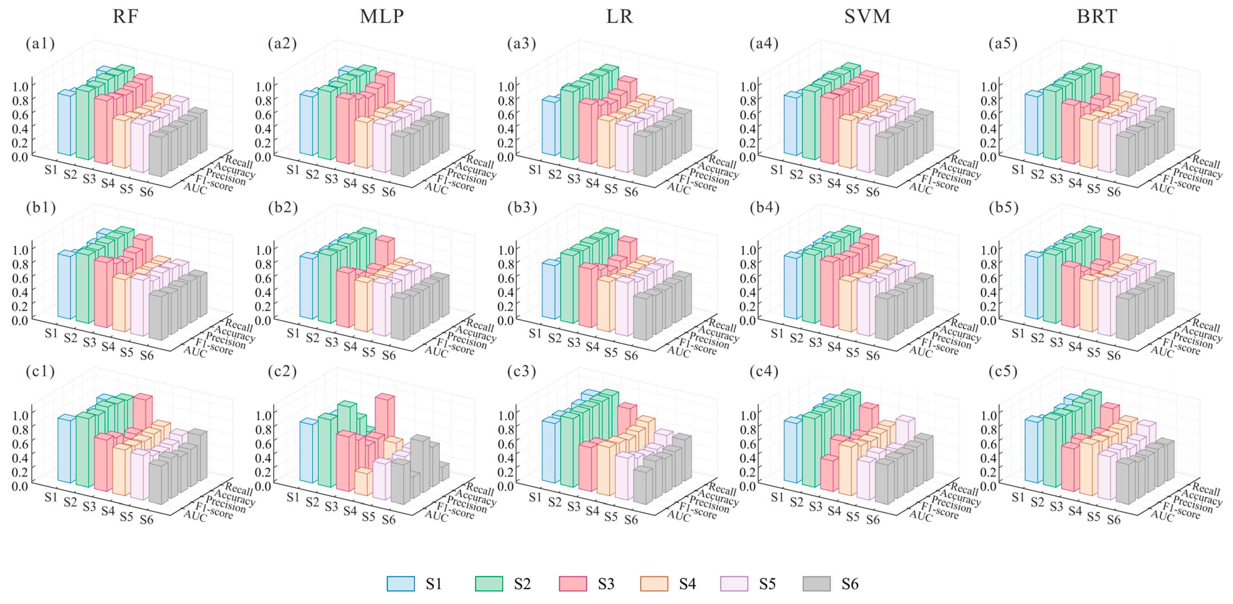
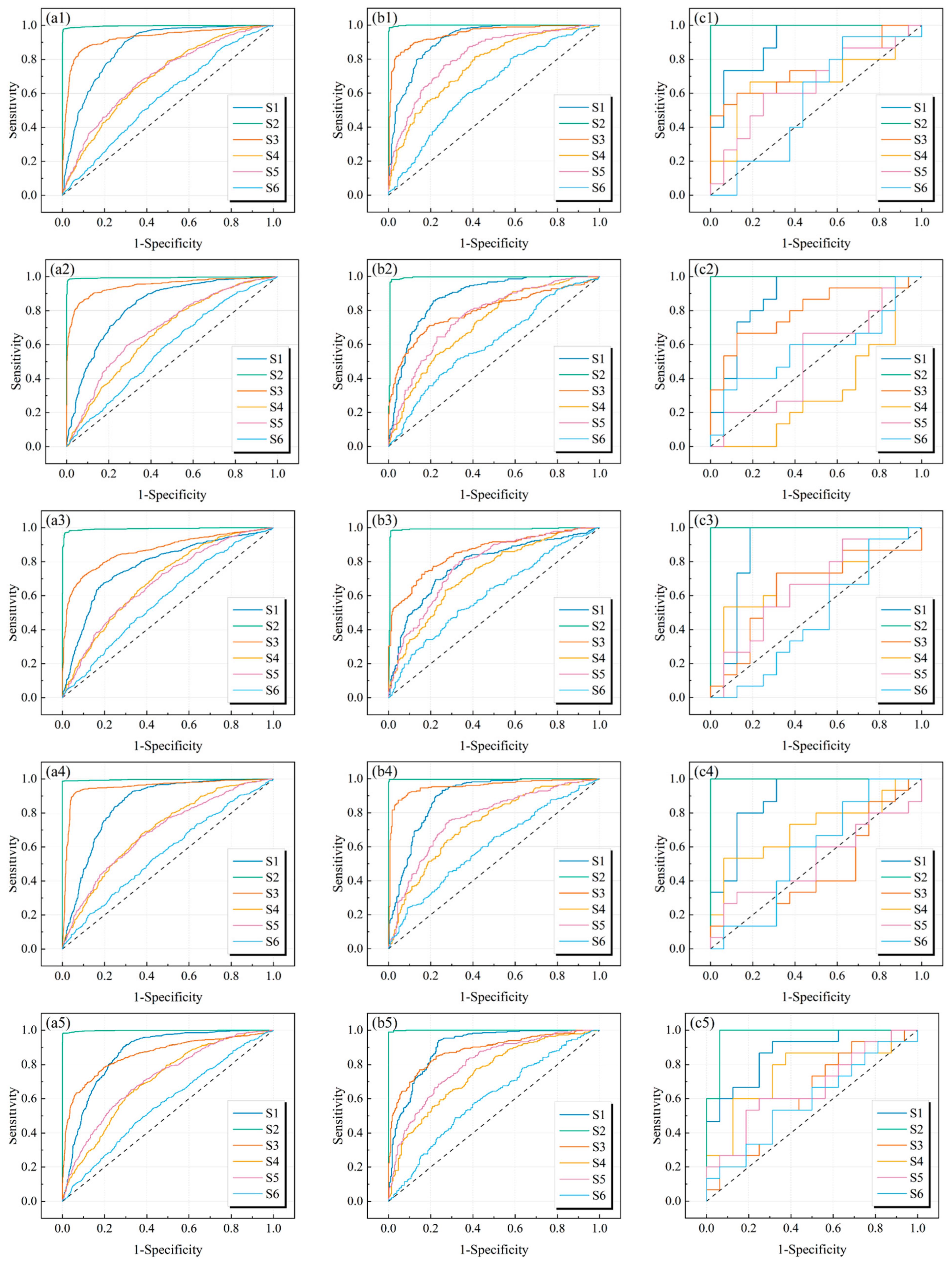
Figure 9 shows the classification performance of different machine learning models for landslide, collapse, and debris-flow susceptibility modeling under the six negative-sample selection strategies. To further evaluate the discriminative ability of different negative-sample selection strategies, the ROC curves of the five machine learning models were plotted for landslide, collapse, and debris-flow susceptibility modeling (Figure 10). Table 3 summarizes the mean evaluation metrics of the five machine learning models for each hazard type and negative-sample strategy. Overall, the choice of negative-sample strategy clearly affected model classification performance, and this effect was consistently reflected in AUC, F1-score, precision, accuracy, and recall.

Figure 9. The classification performance of different machine learning models under six negative-sample selection strategies for landslide, collapse, and debris-flow susceptibility modeling: (a1–a5) landslide; (b1–b5) collapse; and (c1–c5) debris flow.

Figure 10. The ROC curves of different machine learning models under six negative-sample selection strategies for landslide, collapse, and debris-flow susceptibility modeling: (a1–a5) landslide; (b1–b5) collapse; and (c1–c5) debris flow.

Table 3. Mean classification performance of the five machine learning models under different negative-sample selection strategies.

Hazard Type	Strategy	AUC	F1-Score	Precision	Accuracy	Recall
Landslide	S1	0.8402	0.7811	0.7698	0.7791	0.7989
	S2	0.9955	0.9813	0.9955	0.9816	0.9676
	S3	0.9100	0.8328	0.7762	0.8126	0.9060
	S4	0.6901	0.6373	0.6321	0.6350	0.6442
	S5	0.6919	0.6542	0.6280	0.6394	0.6827
	S6	0.5739	0.5599	0.5530	0.5546	0.5679
Collapse	S1	0.8733	0.8007	0.7905	0.7993	0.8122
	S2	0.9960	0.9880	0.9956	0.9882	0.9806
	S3	0.8876	0.7870	0.6899	0.7390	0.9288
	S4	0.7386	0.6718	0.6600	0.6664	0.6842
	S5	0.7842	0.7043	0.7263	0.7135	0.6842
	S6	0.6117	0.5773	0.5785	0.5788	0.5763
Debris flow	S1	0.8746	0.7909	0.7650	0.7935	0.8267
	S2	0.9933	0.9139	0.9875	0.9355	0.8800
	S3	0.6525	0.6571	0.5123	0.5355	0.9200
	S4	0.6325	0.5375	0.5169	0.6387	0.5600
	S5	0.5950	0.5535	0.5047	0.5226	0.6267
	S6	0.5517	0.5127	0.5744	0.5548	0.5200

In terms of the overall average performance of the six negative-sample selection strategies, S2 achieved the highest classification performance, with mean AUC, F1-score, precision, accuracy, and recall values of 0.9950, 0.9611, 0.9928, 0.9684, and 0.9427, respectively. This indicates that when negative samples are mainly drawn from regions that are clearly separated from positive samples in feature space, the models can distinguish the two classes more easily and obtain higher classification scores. By contrast, S3 produced mean AUC, F1-score, precision, accuracy, and recall values of 0.8167, 0.7590, 0.6595, 0.6957, and 0.9183, respectively. Although S3 achieved high recall, its precision and accuracy were markedly lower than those of S2. This suggests that when negative samples are mainly selected from regions similar to the positive samples, the models can identify more true hazard samples but are also more likely to misclassify similar background units as hazards, thereby increasing false positives. The proposed S1 strategy maintained more balanced overall classification performance, with mean AUC, F1-score, precision, accuracy, and recall values of 0.8627, 0.7909, 0.7751, 0.7907, and 0.8126, respectively. Compared with the average performance of the other five strategies, S1 improved AUC, F1-score, precision, accuracy, and recall by 14.47%, 12.25%, 12.54%, 12.99%, and 9.52%, respectively.

In addition, the effects of negative-sample selection varied among hazard types. For landslide and debris flow, the performance gaps between S1 and the two buffer-based strategies were particularly pronounced. In the landslide task, S1 achieved mean AUC, F1-score, precision, accuracy, and recall values of 0.8402, 0.7811, 0.7698, 0.7791, and 0.7989, respectively. These values were substantially higher than those of S5, which yielded 0.6919, 0.6542, 0.6280, 0.6394, and 0.6827, and S6, which further declined to 0.5739, 0.5599, 0.5530, 0.5546, and 0.5679. A similar pattern was observed for debris flows. S1 reached 0.8746, 0.7909, 0.7650, 0.7935, and 0.8267 for the five metrics, respectively, clearly outperforming S5 and S6. The corresponding values were 0.5950, 0.5535, 0.5047, 0.5226, and 0.6267 for S5, and 0.5517, 0.5127, 0.5744, 0.5548, and 0.5200 for S6.

In the collapse task, S5 performed closer to S1, although a clear gap remained. S1 achieved mean AUC, F1-score, precision, accuracy, and recall values of 0.8733, 0.8007, 0.7905, 0.7993, and 0.8122, respectively, whereas S5 yielded 0.7842, 0.7043, 0.7263, 0.7135, and 0.6842. This indicates that although S5 retained relatively high precision for collapses, its recall was clearly lower than that of S1, suggesting limited completeness in identifying positive collapse samples. By contrast, S6 remained weak in the collapse task, with values of 0.6117, 0.5773, 0.5785, 0.5788, and 0.5763 for the five metrics, respectively.

4.3. Hazard Susceptibility Mapping

Compared with classification metrics, susceptibility maps provide a more direct representation of spatial variation in hazard proneness and potential hazard-prone zones. Therefore, using the three best-performing models—RF, SVM, and BRT—this study generated susceptibility probabilities for landslide, collapse, and debris-flow hazards for all slope units in the study area. Historical hazard records were then used to calculate the corresponding $C_{10\%}$, $C_{20\%}$, $C_{30\%}$, $A_{50\%}$, and $A_{80\%}$ values, as reported in Table 4, Table 5 and Table 6.

Table 4. Quantitative evaluation of landslide susceptibility maps generated by different models and negative-sample selection strategies.

Model	Sampling Strategy	${\mathit{C}}_{10\mathbf{\%}}$	${\mathit{C}}_{20\mathbf{\%}}$	${\mathit{C}}_{30\mathbf{\%}}$	${\mathit{A}}_{50\mathbf{\%}}$	${\mathit{A}}_{80\mathbf{\%}}-{\mathit{A}}_{50\mathbf{\%}}$	${\mathit{A}}_{80\mathbf{\%}}$
RF	S1	74.67%	82.01%	87.49%	2.01%	16.72%	18.73%
	S2	0.00%	0.00%	25.00%	38.88%	22.37%	61.25%
	S3	12.19%	23.60%	37.36%	39.50%	32.72%	72.22%
	S4	34.02%	56.05%	71.75%	17.20%	19.63%	36.83%
	S5	60.71%	79.28%	86.41%	6.40%	14.45%	20.85%
	S6	71.17%	80.97%	85.21%	3.97%	14.46%	18.43%
SVM	S1	33.94%	49.59%	61.45%	20.32%	31.55%	51.87%
	S2	0.00%	12.77%	22.90%	51.06%	26.41%	77.47%
	S3	27.88%	45.68%	58.48%	23.22%	29.66%	52.88%
	S4	17.75%	32.70%	43.95%	35.31%	31.39%	66.70%
	S5	31.01%	48.64%	62.11%	20.84%	27.62%	48.46%
	S6	20.22%	36.20%	73.43%	25.16%	14.46%	39.62%
BRT	S1	32.25%	50.70%	64.87%	19.60%	25.52%	45.12%
	S2	17.13%	30.31%	43.53%	36.54%	36.26%	72.80%
	S3	21.66%	42.96%	45.84%	30.64%	33.28%	63.92%
	S4	29.00%	46.46%	60.42%	22.15%	29.31%	51.46%
	S5	31.34%	49.38%	62.81%	20.35%	27.84%	48.19%
	S6	28.83%	47.08%	60.67%	21.68%	28.85%	50.53%

Note: $A_{80\%}-A_{50\%}$ indicates the additional proportion of slope units required to increase the hazard-capture rate from 50% to 80%.

Table 5. Quantitative evaluation of collapse susceptibility maps generated by different models and negative-sample selection strategies.

Model	Sampling Strategy	${\mathit{C}}_{10\mathbf{\%}}$	${\mathit{C}}_{20\mathbf{\%}}$	${\mathit{C}}_{30\mathbf{\%}}$	${\mathit{A}}_{50\mathbf{\%}}$	${\mathit{A}}_{80\mathbf{\%}}-{\mathit{A}}_{50\mathbf{\%}}$	${\mathit{A}}_{80\mathbf{\%}}$
RF	S1	79.19%	85.91%	89.33%	1.46%	10.28%	11.74%
	S2	0.00%	0.00%	53.13%	27.63%	31.31%	58.94%
	S3	12.93%	22.63%	34.59%	43.11%	34.59%	77.70%
	S4	53.13%	72.52%	82.22%	8.90%	18.80%	27.70%
	S5	72.31%	84.91%	89.33%	4.75%	9.34%	14.09%
	S6	75.88%	83.13%	88.25%	3.65%	9.21%	12.86%
SVM	S1	43.43%	58.62%	65.73%	13.48%	30.95%	44.43%
	S2	0.32%	11.53%	19.50%	52.70%	23.76%	76.46%
	S3	18.53%	33.19%	46.12%	33.28%	32.34%	65.62%
	S4	21.23%	37.18%	77.37%	23.13%	9.71%	32.84%
	S5	38.58%	57.65%	68.43%	15.10%	32.95%	48.05%
	S6	37.07%	54.96%	67.67%	16.78%	29.27%	46.05%
BRT	S1	45.47%	64.55%	75.11%	11.80%	23.76%	35.56%
	S2	7.54%	43.75%	51.72%	28.26%	38.72%	66.98%
	S3	12.18%	23.17%	37.07%	40.19%	30.64%	70.83%
	S4	35.13%	54.53%	70.91%	17.33%	22.01%	39.34%
	S5	40.09%	58.08%	70.04%	15.15%	26.70%	41.85%
	S6	43.00%	59.16%	71.98%	14.43%	24.23%	38.66%

Note: $A_{80\%}-A_{50\%}$ indicates the additional proportion of slope units required to increase the hazard-capture rate from 50% to 80%.

Table 6. Quantitative evaluation of debris-flow susceptibility maps generated by different models and negative-sample selection strategies.

Model	Sampling Strategy	${\mathit{C}}_{10\mathbf{\%}}$	${\mathit{C}}_{20\mathbf{\%}}$	${\mathit{C}}_{30\mathbf{\%}}$	${\mathit{A}}_{50\mathbf{\%}}$	${\mathit{A}}_{80\mathbf{\%}}-{\mathit{A}}_{50\mathbf{\%}}$	${\mathit{A}}_{80\mathbf{\%}}$
RF	S1	86.27%	90.20%	92.16%	1.88%	5.78%	7.66%
	S2	31.37%	52.94%	64.71%	14.63%	33.30%	47.93%
	S3	25.49%	37.25%	47.06%	31.70%	17.38%	49.08%
	S4	49.02%	68.63%	78.43%	11.08%	22.27%	33.35%
	S5	82.35%	86.27%	88.24%	1.82%	4.68%	6.50%
	S6	74.51%	80.39%	90.20%	0.87%	19.00%	19.87%
SVM	S1	23.53%	84.31%	92.16%	12.70%	2.93%	15.63%
	S2	15.69%	29.41%	39.22%	38.49%	13.85%	52.34%
	S3	5.88%	13.73%	23.53%	59.60%	27.00%	86.60%
	S4	39.22%	60.78%	68.63%	14.95%	30.91%	45.86%
	S5	45.10%	58.82%	66.67%	11.78%	35.20%	46.98%
	S6	0.00%	7.84%	7.84%	94.82%	4.72%	99.54%
BRT	S1	84.31%	86.27%	90.20%	3.47%	2.69%	6.16%
	S2	5.88%	11.76%	15.69%	56.26%	14.39%	70.65%
	S3	25.49%	35.29%	45.10%	32.15%	29.27%	61.42%
	S4	56.86%	74.51%	84.31%	7.98%	19.27%	27.25%
	S5	45.10%	60.78%	84.31%	13.93%	12.55%	26.48%
	S6	74.51%	80.39%	80.39%	2.00%	14.12%	16.12%

Note: $A_{80\%}-A_{50\%}$ indicates the additional proportion of slope units required to increase the hazard-capture rate from 50% to 80%.

For landslide susceptibility mapping, S1 showed strong overall hazard-capture ability and spatial screening efficiency. Taking the RF model as an example, S1 captured 74.67%, 82.01%, and 87.49% of historical landslides within the top 10%, 20%, and 30% high-susceptibility slope units, respectively, and required only 2.01% and 18.73% of slope units to cover 50% and 80% of the historical landslides. The corresponding $A_{80\%}-A_{50\%}$ was 16.72%, indicating that the expansion from the 50% to 80% hazard-capture target remained relatively limited. In contrast, S2 and S3 required much larger total screening extents, with $A_{80\%}$ values of 61.25% and 72.22%, respectively. By contrast, under RF, S2 yielded 0.00% for both $C_{10\%}$ and $C_{20\%}$, and even when the high-susceptibility extent is expanded to the top 30%, it captures only 25.00% of historical landslides, indicating that despite its excellent classification performance, it did not form an effective study area-wide susceptibility ranking. Similarly, in collapse susceptibility mapping, S1 retained a clear advantage in study area-wide mapping. Under the RF model, the $C_{10\%}$, $C_{20\%}$, and $C_{30\%}$ values of S1 are 79.19%, 85.91%, and 89.33%, respectively, with corresponding $A_{50\%}$ and $A_{80\%}$ values of only 1.46% and 11.74%. Its $A_{80\%}-A_{50\%}$ was 10.28%, showing that only a small additional screening extent was needed after 50% of the collapse records had been captured. The RF results of S5 and S6 were also close to S1 in terms of $A_{80\%}-A_{50\%}$ with values of 9.34% and 9.21%, respectively, which is consistent with their relatively similar mapping performance in the collapse task. Notably, S5 yields 72.31%, 84.91%, and 89.33%, and S6 yields 75.88%, 83.13%, and 88.25%, meaning that their mapping performance is relatively close to that of S1. However, when the SVM and BRT results are considered jointly, the proposed S1 exhibited more stable spatial screening efficiency. Its mean $A_{50\%}$ and $A_{80\%}$ are 12.64% and 40.00%, both clearly better than the mean performance of the buffer-related strategies S5 and S6, which are 15.37% and 43.65%, respectively.

Owing to the limited number of historical debris-flow samples, the study area-wide susceptibility ranking is more sensitive to variations in negative-sample selection strategy. Overall, S1 showed strong hazard-capture ability under both RF and BRT, with the corresponding $C_{10\%}$ values reaching 86.27% and 84.31%, and $A_{80\%}$ values of only 7.66% and 6.16%. The corresponding $A_{80\%}-A_{50\%}$ values were 5.78% and 2.69%, respectively, indicating that the 80% hazard-capture target could be reached with only a limited expansion beyond the 50% capture area. By contrast, S2 and S3 required much larger $A_{80\%}$ values under most models, suggesting lower spatial screening efficiency despite their feature-space separation effects. Although the $C_{10\%}$ of S1 under the SVM model is only 23.53%, the capture rate rises rapidly to 84.31% and 92.16% when the high-susceptibility range is expanded to the top 20% and 30%, indicating that the strategy can still achieve high hazard concentration within a limited spatial extent. By contrast, S5 and S6 are more strongly model-dependent in the debris-flow task. In particular, S6 under SVM almost lost effective ranking ability, with $C_{10\%}$, $C_{20\%}$, and $C_{30\%}$ of only 0.00%, 7.84%, and 7.84%, respectively, and $A_{50\%}$ and $A_{80\%}$ as high as 94.82% and 99.54%. Its $A_{80\%}-A_{50\%}$ was only 4.72%, but this was mainly because its $A_{50}$ had already reached 94.82%, indicating that most of the study area had to be included before a meaningful hazard-capture level could be achieved.

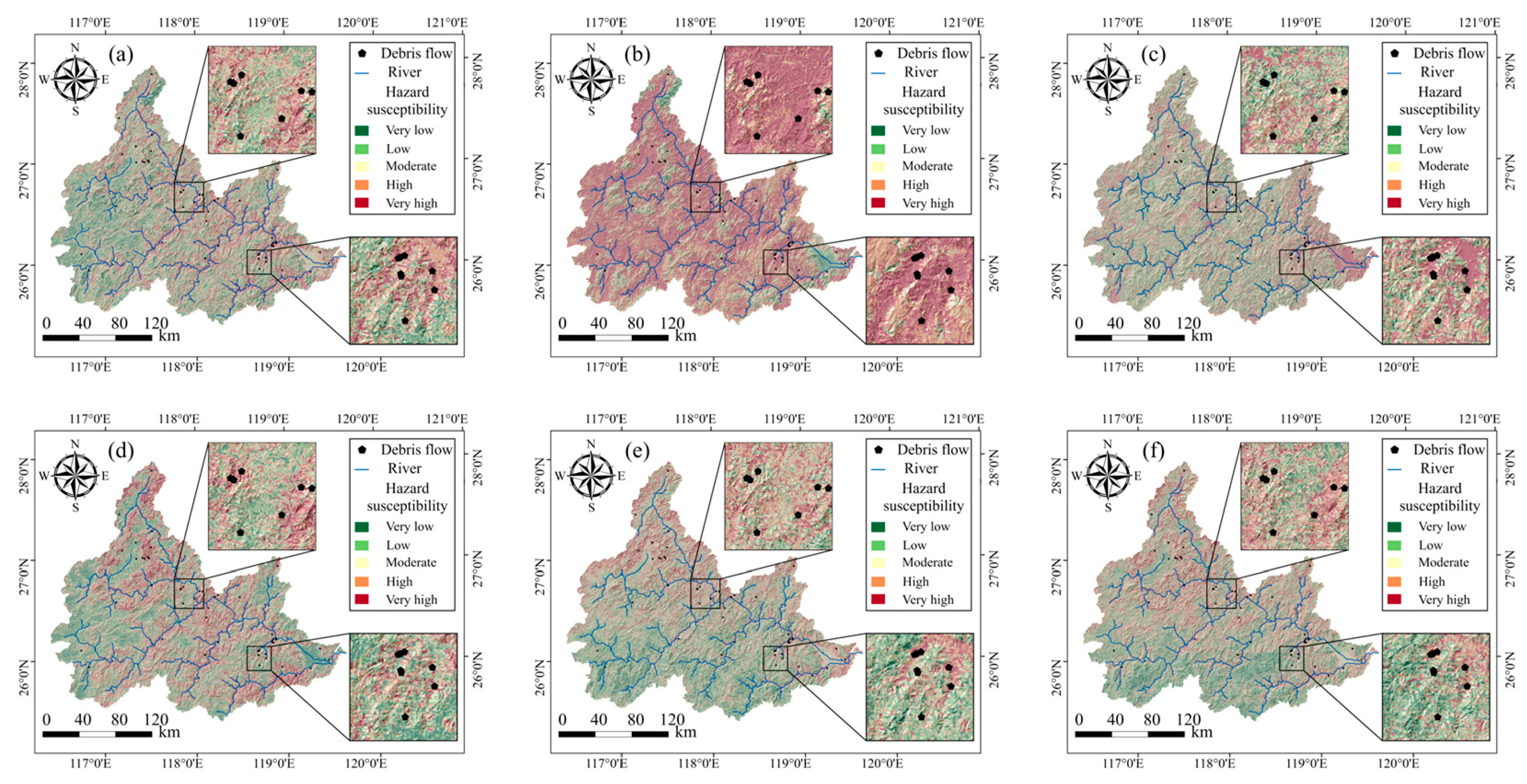
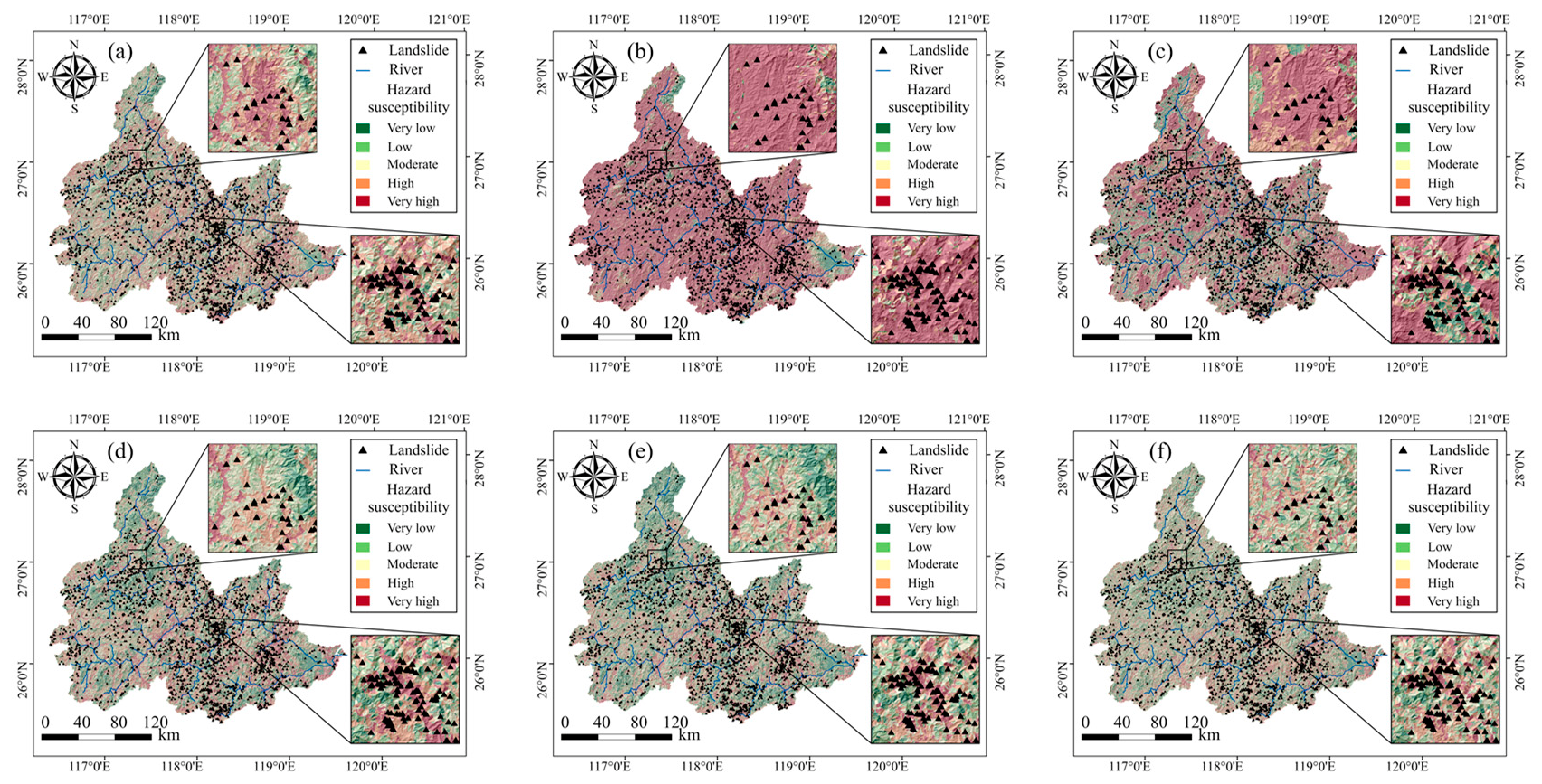
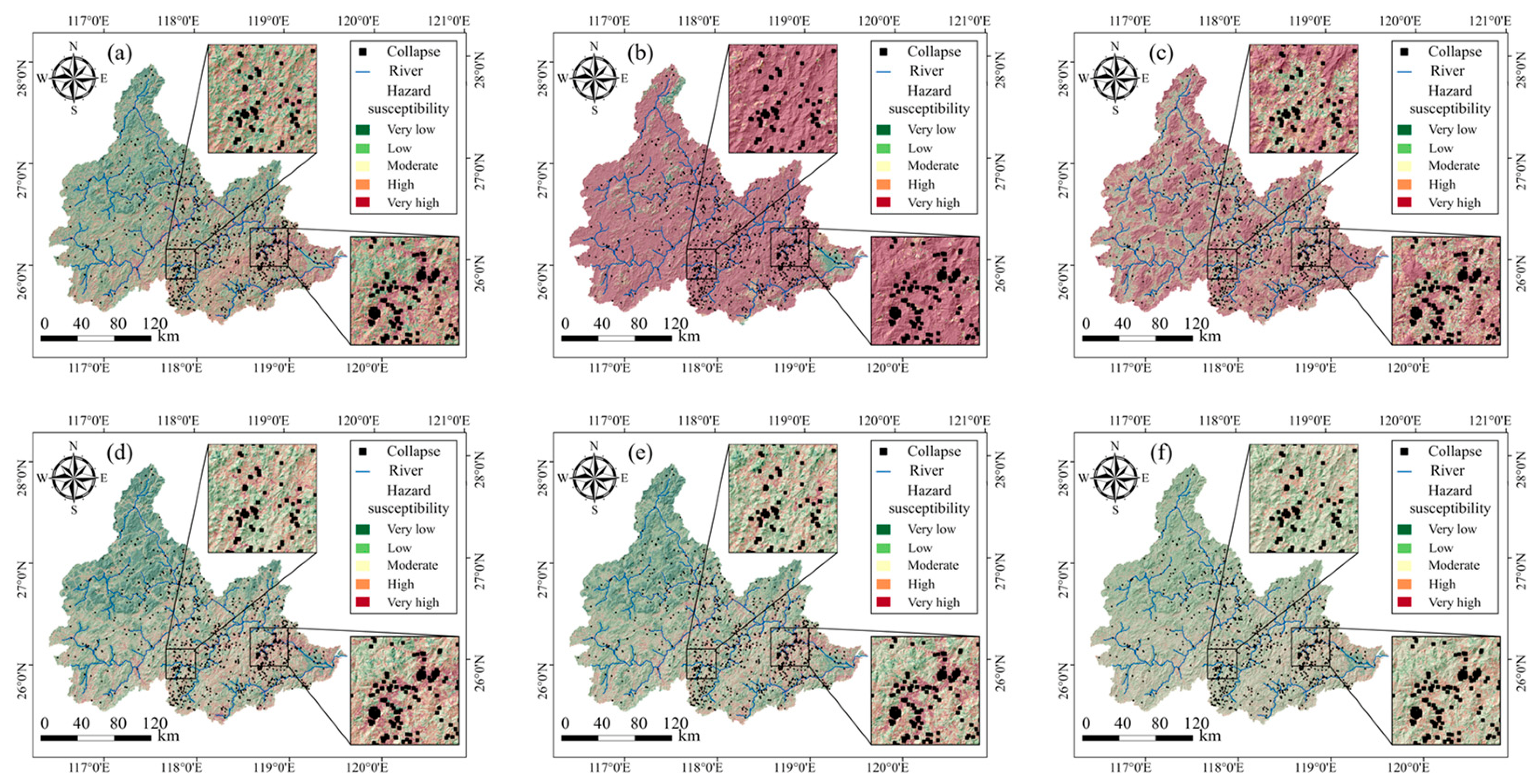
Considering the above classification and mapping-quality results together, the RF model showed high hazard-capture ability and relatively stable spatial ranking for all three hazard types. Therefore, RF was selected as the representative model to display susceptibility maps for landslide, collapse, and debris flow under different negative-sample strategies (Figure 11, Figure 12 and Figure 13).

Figure 11. Landslide susceptibility maps generated by the RF model under six negative-sample selection strategies: (a) S1; (b) S2; (c) S3; (d) S4; (e) S5; and (f) S6.

Figure 12. Collapse susceptibility maps generated by the RF model under six negative-sample selection strategies: (a) S1; (b) S2; (c) S3; (d) S4; (e) S5; and (f) S6.

Figure 13. Debris-flow susceptibility maps generated by the RF model under six negative-sample selection strategies: (a) S1; (b) S2; (c) S3; (d) S4; (e) S5; and (f) S6.

The susceptibility maps of the three hazard types generated by the RF model showed that different negative-sample strategies substantially altered the spatial organization of high-susceptibility zones and their correspondence with historical hazard points. Overall, S1 exhibited relatively stable spatial performance in landslide, collapse, and debris-flow mapping. Its high-susceptibility zones are mainly concentrated in areas with dense historical hazard points and their adjacent slope or channel units, thereby covering the major hazard clusters while avoiding excessive expansion of high-susceptibility areas. In contrast, although S2 achieved the highest sample-level classification performance, its susceptibility maps showed extensive high-value expansion, with high-susceptibility zones extending broadly across the study area. This pattern was particularly evident in the landslide and collapse maps, where broad and continuous high-susceptibility patches were observed. This suggests that although distant negative samples enhance the separability between positive and negative samples during training, they may lead the model to overestimate the risk of background slope units during full-area prediction, thereby weakening the ability of high-susceptibility zones to spatially screen true hazard clusters. S3, S4, S5, and S6 showed varying degrees of spatial fragmentation, local over-contraction, or discontinuous high-susceptibility patches. Among them, S5 and S6 exhibited spatial patterns relatively close to S1 in the collapse task, indicating a certain degree of applicability. However, their stability is insufficient in the landslide and debris-flow tasks, particularly when the number of debris-flow samples is limited, where the high-susceptibility zones are more sensitive to the form of spatial constraints imposed during negative-sample selection.

Overall, the performance of different negative-sample selection strategies is not consistent across classification performance and study area-wide susceptibility mapping. Although S2 performed best in classification, it suffers from serious deficiencies in hazard-capture ability within high-susceptibility areas in hazard mapping, especially for landslides. S3 can increased the discriminative difficulty between positive and negative samples, but its mapping performance is strongly affected by model type and is difficult to stabilize across hazards. S5 and S6 showed some effectiveness in the collapse task, but their stability remains insufficient in the landslide and debris-flow tasks, with particularly pronounced fluctuations in small-sample debris-flow mapping. By contrast, although S1 did not achieve the highest value on every individual metric, it consistently maintained high hazard-capture rates and low area requirements across landslide, collapse, and debris flow, thereby exhibiting more stable study area-wide mapping ability.

5. Discussion

5.1. Mechanisms by Which Negative-Sample Selection Shapes Model Decision Boundaries

In this study, when the hazard type, conditioning-factor system, and prediction model were held constant, changing only the negative-sample selection strategy led to clear differences in AUC, F1-score, precision, accuracy, and recall. This indicates that negative-sample selection is not merely a preprocessing step, but a key factor shaping the classification boundary of susceptibility models [18,19].

From the perspective of negative-sample construction, S4, S5, and S6 are all non-feature-adaptive strategies. S4 emphasizes the overall representativeness of candidate background samples, based on the implicit assumption that, after known hazard units are excluded, the remaining background samples can collectively represent non-hazard conditions. This strategy is easy to implement and avoids imposing strong prior constraints, which explains its widespread use in susceptibility-mapping studies. However, background areas without recorded hazards are not equivalent to homogeneous stable regions; they may still contain slope units that are highly similar to the positive samples of the target hazard [55,56]. S5 and S6 can be regarded as spatially constrained variants of S4. By excluding areas adjacent to known hazards or restricting sampling to a buffer ring, they attempt to reduce the likelihood that near-hazard background units are mistakenly selected as negative samples. However, their underlying assumptions remain idealized: slope units far from known hazards, or located within a specific buffer ring, are assumed to have more suitable negative-sample characteristics. In fact, slope-instability processes are not controlled by spatial distance alone. The same buffer distance may correspond to very different environmental contexts under different geomorphic positions, gully systems, road-disturbance conditions, and lithological settings [57]. Moreover, S5 and S6 remain fundamentally stochastic spatial-sampling strategies and cannot explicitly represent the feature-space distance or discriminative difficulty between candidate negative samples and the positive samples of different hazards. Consequently, in a multi-hazard susceptibility-mapping context, these strategies may limit the model’s ability to learn hazard-specific environmental differences, thereby weakening robustness and generalization [58].

Therefore, the key to negative-sample selection lies in determining what discriminative information candidate background units can provide in environmental feature space, rather than simply moving samples away from hazard locations. For machine learning models, decision boundaries are shaped by the distributional relationships among samples in feature space, not merely by their spatial proximity. This explains the contrasting classification performance of S2 and S3 observed in this study. By selecting background units far from the positive-sample distribution, S2 increased feature separability between positive and negative samples and thus achieved high AUC, precision, and accuracy, with mean values of 0.9949, 0.9929, and 0.9684 across the three hazards, respectively. Conversely, S3 selected background units closer to the positive-sample distribution, which increases decision-boundary learning difficulty and yields higher recall but lower precision and accuracy. Compared with S2, the precision and accuracy of S3 decreased by 33.58% and 28.16%, respectively.

However, if negative-sample construction relies exclusively on one extreme of feature-space distance, the resulting decision boundary may become biased toward a single discrimination pattern. For this reason, the proposed S1 strategy does not rely solely on easy or hard negatives. Instead, it combines typical background samples that are clearly distinct from hazard samples, boundary-adjacent samples that are close to positive samples, and randomly supplemented background samples that help maintain overall representativeness. Its core advantage is that it improves the fit between negative samples and the target hazard-classification task while keeping discriminative difficulty within a reasonable range. Accordingly, S1 produced more balanced AUC, F1-score, Precision, Accuracy, and Recall in the present results, suggesting that composite negative-sample construction can provide a stable balance among sample separability, boundary discrimination, and background representativeness.

5.2. Inconsistency Between Classification Performance and Study Area-Wide Mapping Quality

An inconsistency may exist between classification performance and study area-wide mapping quality. Although AUC, F1-score, and related metrics are widely used to evaluate the discriminative ability of susceptibility models, previous studies have shown that classification performance is not directly equivalent to susceptibility-map quality, which also depends on spatial transferability and predictive uncertainty [27]. In other words, high classification scores do not necessarily guarantee susceptibility maps with equally strong hazard-capture ability.

The results of this study further confirm the existence of this inconsistency. Although S2 achieved the highest mean AUC, F1-score, precision, accuracy, and recall, its classification advantage did not consistently translate into better spatial capture of hazards across the study area. In study area-wide susceptibility mapping, the model is not applied to an idealized binary sample set, but to a continuous landscape of slope units that includes intermediate states, boundary-similar background units, and complex environmental combinations. When S2 is trained mainly on background units far from the positive-sample distribution, the model may become overly dependent on strong feature contrasts between positive and negative samples. This can weaken its ability to rank intermediate-gradient and boundary-similar slope units by susceptibility probability. For example, in the RF landslide model, S2 captured no historical landslides within either the top 10% or top 20% high-susceptibility areas, and captured only 25.00% of historical landslides even when the high-susceptibility area was expanded to the top 30%. This result shows that strong sample-level classification performance does not necessarily lead to effective study area-wide hazard ranking. The area-based indicators further support this interpretation: under the RF landslide model, S2 required 61.25% of slope units to capture 80% of the historical landslides, whereas S1 required only 18.73%. This difference indicates that high classification separability may still lead to an inefficient spatial screening pattern when the trained model is applied to all slope units.

By contrast, the advantage of the proposed S1 strategy does not lie in achieving an extreme optimum for a single metric, but in establishing a more stable balance between classification discrimination and study area-wide susceptibility ranking. Unlike S2, S1 does not rely solely on distant background samples to artificially enlarge class separability. Although its classification performance is lower than that of S2, S1 better preserves the model’s ability to identify susceptibility in complex transitional zones. Unlike S3, S5, and S6, S1 also avoids overconcentrating negative samples in boundary-adjacent areas, boundary-similar zones, or predefined distance ranges. This reduces the likelihood that the model decision boundary becomes biased toward a single sample structure. As a result, S1 achieved relatively balanced performance in terms of hazard capture rate, required area proportion, and classification discrimination, demonstrating greater stability for study area-wide susceptibility mapping. In practical terms, lower $A_{50}$, $A_{80}-A_{50}$, and $A_{80}$ values indicate that a given proportion of known hazards can be captured within a narrower priority screening area, which is more useful for regional risk screening and prioritizing field investigation or mitigation resources.

5.3. Hazard Adaptability of Negative-Sample Strategies and Differences in Feature Space

In multi-hazard susceptibility mapping, landslide, collapse, and debris flow can all be treated as slope-instability hazards and are therefore often modeled within a unified feature space [5]. However, differences in triggering mechanisms, occurrence frequency, and environmental controls among these hazards cannot be ignored [6,59]. Negative samples should therefore not be regarded as a single stable background shared across hazard types, but as background samples associated with specific hazard-discrimination tasks.

This point is clearly reflected in the feature-space distributions produced by different negative-sample selection strategies. S2 produced distributions far from the positive samples for all three hazards (Figure 6b, Figure 7b and Figure 8b), indicating that it mainly selected distant background samples that were strongly differentiated from the hazard samples. By contrast, S6 showed clearer adjacency and overlap with the positive samples (Figure 6f, Figure 7f and Figure 8f), suggesting that its negative samples were closer to the environmental feature range occupied by the hazard samples. S3, S4, and S5 showed intermediate feature-space structures, rather than forming either a purely distant separation pattern or a highly overlapping structure (Figure 6c–e, Figure 7c–e and Figure 8c–e). These results indicate that different negative-sample selection strategies substantially alter the relative relationship between positive and negative samples in feature space.

Notably, S3, as a hard negative-sample strategy based on feature-space distance, was expected to select samples closer to the positive samples; however, its Mean |SMD| was not the lowest among all strategies. This phenomenon is likely related to its centroid-based screening criterion. Specifically, S3 selects candidate background samples according to their distance from the centroid of the positive-sample distribution. For hazard samples with dispersed feature-space distributions, proximity to the mean centroid does not necessarily indicate the highest similarity across all conditioning-factor dimensions. Consequently, some background samples located close to the centroid may still differ substantially from certain parts of the positive-sample distribution, resulting in a Mean |SMD| value that is not the lowest among the six strategies.

Compared with the fixed-logic sampling strategies discussed above, the proposed S1 strategy showed stronger hazard-specific adaptability. It remained relatively close to the positive samples for landslide and collapse but formed a more clearly separated overall structure for debris flow (Figure 6a, Figure 7a and Figure 8a). This indicates that S1 did not impose a fixed negative-sample distance pattern across the three hazards. Instead, it formed hazard-specific combinations of negative samples according to the distributional characteristics of the positive samples for each hazard. For landslide and collapse, retaining a certain number of boundary-adjacent samples helped preserve the model’s ability to discriminate similar slope environments. For debris flow, where the sample size was smaller and the feature-space distribution was less stable, stronger background separation helped to prevent negative samples from becoming overly concentrated around the positive samples.

5.4. Limitations and Future Work

This study has several limitations that warrant further investigation. First, a 1:1 positive-to-negative sample ratio was adopted to ensure a controlled comparison among different negative-sample selection strategies. Although this setting helps isolate the effect of sampling strategy, regional geohazard occurrence is usually highly imbalanced, and differences in inventory size among hazard types may affect positive-sample centroid estimation and feature-space distance ranking, especially for small-sample hazards such as debris flows. Therefore, the mapping performance of the proposed strategy under different sample ratios and inventory sizes should be further examined. Second, Euclidean distance was used to rank candidate background samples in standardized feature space. This metric is consistent with the centroid-based framework, but alternative distance measures may produce different rankings and negative-sample sets. Additional, the method was evaluated only in the Minjiang River Basin. Its applicability and robustness should be further tested under different regional settings and modeling architectures, including deep learning-based susceptibility models.

Finally, the debris-flow inventory was available as point-based records rather than event polygons or process-zone delineations. Consequently, labeling only the slope unit containing the recorded point may not fully represent the spatial extent and environmental heterogeneity of the event. Moreover, if inventory points are preferentially located in a particular geomorphic position, such as the depositional zone near settlements or infrastructure, the derived positive-sample distribution may be biased toward the corresponding topographic and hydrological conditions. This positional uncertainty may affect the estimated positive-sample centroid, the feature-space ranking of candidate negative samples, and the resulting debris-flow susceptibility pattern. The absence of detailed event boundaries and process-zone attributes prevents a complete evaluation of this uncertainty. Future studies should incorporate polygon-based debris-flow inventories and explicitly distinguish source, transport, and deposition zones when sufficient field and remote-sensing information becomes available.

6. Conclusions

This study developed a task-specific negative-sample selection method for multi-hazard susceptibility mapping of landslides, collapses, and debris flows. The main findings are as follows:

(1) The proposed method generated hazard-specific negative-sample structures, with Mean |SMD| values of 0.09, 0.13, and 0.69 for landslides, collapses, and debris flows, respectively.

(2) Compared with the mean performance of the five benchmark strategies, the proposed method increased AUC and F1-score by 14.47% and 12.25%, respectively, while maintaining a better balance between sample-level classification and study area-wide susceptibility ranking.

(3) The top 10% of susceptible slope units captured 39.26% of historical hazard events, and 27.06% of the slope units were required to capture 80% of the events.

Overall, the results highlight the importance of hazard-specific negative-sample construction in regional multi-hazard susceptibility mapping.

References

- Godes, C.R.; Lim, O.-B.; Rodrigazo, S.A.; Kim, Y.; Kim, Y.; Lee, S.; Yeon, J. Advancing geohazard risk assessment—A digital tool for steep slope management. Prog. Disaster Sci. 2025, 26, 100418. [Google Scholar] [CrossRef] [Scilit]
- Gbadebo, A.M.; Adedeji, O.H.; Edogbo, A.S. GIS-based landslide susceptibility assessment in Eyinoke Hilly Area of Okeigbo, SW, Nigeria. J. Appl. Sci. Environ. Manag. 2018, 22, 917–924. [Google Scholar] [CrossRef] [Scilit]
- Froude, M.J.; Petley, D.N. Global fatal landslide occurrence from 2004 to 2016. Nat. Hazards Earth Syst. Sci. 2018, 18, 2161–2181. [Google Scholar] [CrossRef] [Scilit]
- Cao, J.; Zhang, Z.; Du, J.; Zhang, L.; Song, Y.; Sun, G. Multi-geohazards susceptibility mapping based on machine learning—A case study in Jiuzhaigou, China. Nat. Hazards 2020, 102, 851–871. [Google Scholar] [CrossRef] [Scilit]
- Zhang, Q.; Ma, W.; Gao, Y.; Zhang, T.; Ma, X.; Li, L.; Zhou, Q.; Liu, F. Zoning of the Disaster-Inducing Environment and Driving Factors for Landslides, Collapses, and Debris Flows on the Qinghai–Tibet Plateau. Appl. Sci. 2025, 15, 6569. [Google Scholar] [CrossRef] [Scilit]
- Hungr, O.; Leroueil, S.; Picarelli, L. The Varnes classification of landslide types, an update. Landslides 2014, 11, 167–194. [Google Scholar]
- Iverson, R.M. The physics of debris flows. Rev. Geophys. 1997, 35, 245–296. [Google Scholar] [CrossRef] [Scilit]
- Benda, L.; Dunne, T. Stochastic forcing of sediment supply to channel networks from landsliding and debris flow. Water Resour. Res. 1997, 33, 2849–2863. [Google Scholar] [CrossRef] [Scilit]
- He, K.; Chen, X.; Yu, X.; Dong, C.; Zhao, D. Evaluation and prediction of compound geohazards in highly urbanized regions across China’s Greater Bay Area. J. Clean. Prod. 2024, 449, 141641. [Google Scholar] [CrossRef] [Scilit]
- Kim, C.; Park, S.; Han, H. Multi-Hazard susceptibility mapping using machine learning approaches: A case study of South Korea. Remote Sens. 2025, 17, 1660. [Google Scholar] [CrossRef] [Scilit]
- Pourhashemi, S.; Asadi, M.A.Z.; Boroughani, M. Multi-hazard susceptibility mapping in the Salt Lake watershed. Environ. Chall. 2025, 18, 101079. [Google Scholar] [CrossRef] [Scilit]
- Liu, S.; Wang, L.; Zhang, W.; He, Y.; Pijush, S. A comprehensive review of machine learning-based methods in landslide susceptibility mapping. Geol. J. 2023, 58, 2283–2301. [Google Scholar] [CrossRef] [Scilit]
- Liu, S.; Wang, L.; Zhang, W.; He, Y.; Pijush, S. Multi-hazard susceptibility mapping based on Convolutional Neural Networks. Geosci. Front. 2022, 13, 101425. [Google Scholar] [CrossRef] [Scilit]
- Ye, P.; Yu, B.; Chen, W.; Feng, Y.; Zhou, H.; Luo, X.; Li, Y. Risk assessment of landslide and rockfall hazards in hilly region of southwestern China: A case study of Qijiang, Wuxi and Chishui. Environ. Earth Sci. 2024, 83, 398. [Google Scholar] [CrossRef] [Scilit]
- Youssef, A.M.; Mahdi, A.M.; Al-Katheri, M.M.; Pouyan, S.; Pourghasemi, H.R. Multi-hazards (landslides, floods, and gully erosion) modeling and mapping using machine learning algorithms. J. Afr. Earth Sci. 2023, 197, 104788. [Google Scholar] [CrossRef] [Scilit]
- Dai, Z.; Fang, J.; Yang, W.; Bai, Z.; Lin, D.; Zhou, L.; Tang, M. Multi-geohazard susceptibility assessment and influencing factors in Zhejiang Province, China: A machine learning approach. Geomat. Nat. Hazards Risk 2026, 17, 2617015. [Google Scholar] [CrossRef] [Scilit]
- Guo, Z.; Tian, B.; Zhu, Y.; He, J.; Zhang, T. How do the landslide and non-landslide sampling strategies impact landslide susceptibility assessment?—A catchment-scale case study from China. J. Rock. Mech. Geotech. Eng. 2024, 16, 877–894. [Google Scholar] [CrossRef] [Scilit]
- Gu, T.; Duan, P.; Wang, M.; Li, J.; Zhang, Y. Effects of non-landslide sampling strategies on machine learning models in landslide susceptibility mapping. Sci. Rep. 2024, 14, 7201. [Google Scholar] [CrossRef] [Scilit] [PubMed]
- Dou, H.; He, J.; Huang, S.; Jian, W.; Guo, C. Influences of non-landslide sample selection strategies on landslide susceptibility mapping by machine learning. Geomat. Nat. Hazards Risk 2023, 14, 2285719. [Google Scholar] [CrossRef] [Scilit]
- Ye, C.; Tang, R.; Wei, R.; Guo, Z.; Zhang, H. Generating accurate negative samples for landslide susceptibility mapping: A combined self-organizing-map and one-class SVM method. Front. Earth Sci. 2023, 10, 1054027. [Google Scholar] [CrossRef] [Scilit]
- Wang, J.; Wang, Z.; Li, M.; Qi, Z.; Cheng, L.; Qi, H.; Zhang, X. Improved landslide susceptibility assessment: A new negative sample collection strategy and a comparative analysis of zoning methods. Ecol. Indic. 2024, 169, 112948. [Google Scholar] [CrossRef] [Scilit]
- Lu, Y.; Xu, H.; Wang, C.; Yan, G.; Huo, Z.; Peng, Z.; Liu, B.; Xu, C. A novel strategy coupling optimised sampling with heterogeneous ensemble machine-learning to predict landslide susceptibility. Remote Sens. 2024, 16, 3663. [Google Scholar] [CrossRef] [Scilit]
- Rabby, Y.W.; Li, Y.; Hilafu, H. An objective absence data sampling method for landslide susceptibility mapping. Sci. Rep. 2023, 13, 1740. [Google Scholar] [CrossRef] [Scilit] [PubMed]
- Liu, L.-L.; Zhao, S.-L.; Yang, C.; Zhang, W. Quantifying uncertainty in landslide susceptibility mapping due to sampling randomness. Int. J. Disaster Risk Reduct. 2024, 114, 104966. [Google Scholar] [CrossRef] [Scilit]
- Zhu, A.-X.; Miao, Y.; Liu, J.; Bai, S.; Zeng, C.; Ma, T.; Hong, H. A similarity-based approach to sampling absence data for landslide susceptibility mapping using data-driven methods. Catena 2019, 183, 104188. [Google Scholar] [CrossRef] [Scilit]
- Chen, S.; Miao, Z.; Wu, L.; Zhang, A.; Li, Q.; He, Y. A one-class-classifier-based negative data generation method for rapid earthquake-induced landslide susceptibility mapping. Front. Earth Sci. 2021, 9, 609896. [Google Scholar] [CrossRef] [Scilit]
- Steger, S.; Brenning, A.; Bell, R.; Petschko, H.; Glade, T. Exploring discrepancies between quantitative validation results and the geomorphic plausibility of statistical landslide susceptibility maps. Geomorphology 2016, 262, 8–23. [Google Scholar] [CrossRef] [Scilit]
- Crawford, M.M.; Koch, H.J.; Dortch, J.M. Evaluating map quality and model performance through iterative statistics-based landslide susceptibility in eastern KY. Nat. Hazards 2025, 121, 11633–11661. [Google Scholar] [CrossRef] [Scilit]
- Lu, Y.; Wang, Y.; Liu, Q.; Chen, X.; Zhang, Y.; Gao, L.; Chen, Y.; Liu, M.; Deng, H. Evapotranspiration variations of the Minjiang River Basin in Southeastern China from 2000 to 2019. Atmosphere 2022, 13, 562. [Google Scholar] [CrossRef] [Scilit]
- Li, X.; Chen, X.; Yang, T.; Tang, Z.; Wen, Z.; Meng, B. Projection of extreme precipitation in the Minjiang river basin, Southeast China. J. Water Clim. Change 2022, 13, 4177–4193. [Google Scholar] [CrossRef] [Scilit]
- Chen, C.; Fan, L. Selection of contributing factors for predicting landslide susceptibility using machine learning and deep learning models. Stoch. Environ. Res. Risk Assess. 2025, 39, 4169–4194. [Google Scholar]
- Meena, S.R.; Puliero, S.; Bhuyan, K.; Floris, M.; Catani, F. Assessing the importance of conditioning factor selection in landslide susceptibility for the province of Belluno (region of Veneto, northeastern Italy). Nat. Hazards Earth Syst. Sci. 2022, 22, 1395–1417. [Google Scholar] [CrossRef] [Scilit]
- Ahmad, H.; Alam, M.; Yinghua, Z.; Najeh, T.; Gamil, Y.; Hameed, S. Landslide risk assessment integrating susceptibility, hazard, and vulnerability analysis in Northern Pakistan. Discov. Appl. Sci. 2024, 6, 7. [Google Scholar] [CrossRef] [Scilit]
- Al-kordi, H.; Al-Amri, A. Landslide susceptibility mapping using geospatial, analytical hierarchy process (AHP), and binary logistic regression (BLR) techniques—A study of Wadi Habban Basin, Shabwah, Yemen. Results Earth Sci. 2025, 3, 100103. [Google Scholar] [CrossRef] [Scilit]
- Wang, H.; Zhu, J.; Chen, L.; Shi, H. Incorporating Dynamic Factors in Geological Hazard Risk Assessment: Integrating InSAR Deformation and Rainfall Conditions. Atmosphere 2025, 16, 360. [Google Scholar] [CrossRef] [Scilit]
- Carrara, A.; Cardinali, M.; Detti, R.; Guzzetti, F.; Pasqui, V.; Reichenbach, P. GIS techniques and statistical models in evaluating landslide hazard. Earth Surf. Processes Landf. 1991, 16, 427–445. [Google Scholar] [CrossRef] [Scilit]
- Guzzetti, F.; Carrara, A.; Cardinali, M.; Reichenbach, P. Landslide hazard evaluation: A review of current techniques and their application in a multi-scale study, Central Italy. Geomorphology 1999, 31, 181–216. [Google Scholar] [CrossRef] [Scilit]
- Ba, Q.; Chen, Y.; Deng, S.; Yang, J.; Li, H. A comparison of slope units and grid cells as mapping units for landslide susceptibility assessment. Earth Sci. Inform. 2018, 11, 373–388. [Google Scholar] [CrossRef] [Scilit]
- Deng, N.; Li, Y.; Ma, J.; Shahabi, H.; Hashim, M.; de Oliveira, G.; Chaeikar, S.S. A comparative study for landslide susceptibility assessment using machine learning algorithms based on grid unit and slope unit. Front. Environ. Sci. 2022, 10, 1009433. [Google Scholar] [CrossRef] [Scilit]
- Alvioli, M.; Marchesini, I.; Reichenbach, P.; Rossi, M.; Ardizzone, F.; Fiorucci, F.; Guzzetti, F. Automatic delineation of geomorphological slope units with r. slopeunits v1. 0 and their optimization for landslide susceptibility modeling. Geosci. Model Dev. 2016, 9, 3975–3991. [Google Scholar] [CrossRef] [Scilit]
- Hong, H.; Miao, Y.; Liu, J.; Zhu, A.-X. Exploring the effects of the design and quantity of absence data on the performance of random forest-based landslide susceptibility mapping. Catena 2019, 176, 45–64. [Google Scholar] [CrossRef] [Scilit]
- Chen, H.; Ma, T.; Shen, L.; Ye, B.; Ni, S.; Ni, X.; Sun, H. Negative sample selection for landslide susceptibility prediction: A hybrid optimization approach using an AHP-KDE multi-ring sampling strategy. Ecol. Indic. 2025, 180, 114304. [Google Scholar] [CrossRef] [Scilit]
- Breiman, L. Random forests. Mach. Learn. 2001, 45, 5–32. [Google Scholar] [CrossRef] [Scilit]
- Breiman, L. Bagging predictors. Mach. Learn. 1996, 24, 123–140. [Google Scholar] [CrossRef] [Scilit]
- Belgiu, M.; Drăguţ, L. Random forest in remote sensing: A review of applications and future directions. ISPRS J. Photogramm. Remote Sens. 2016, 114, 24–31. [Google Scholar] [CrossRef] [Scilit]
- Aggarwal, C.C. Neural Networks and Deep Learning; Springer: Cham, Switzerland, 2018. [Google Scholar]
- Alzubaidi, L.; Zhang, J.; Humaidi, A.J.; Al-Dujaili, A.; Duan, Y.; Al-Shamma, O.; Santamaría, J.; Fadhel, M.A.; Al-Amidie, M.; Farhan, L. Review of deep learning: Concepts, CNN architectures, challenges, applications, future directions. J. Big Data 2021, 8, 53. [Google Scholar] [CrossRef] [Scilit] [PubMed]
- Cox, D.R. The regression analysis of binary sequences. J. R. Stat. Soc. Ser. B Stat. Methodol. 1958, 20, 215–232. [Google Scholar] [CrossRef] [Scilit]
- James, G.; Witten, D.; Hastie, T.; Tibshirani, R. An Introduction to Statistical Learning: With Applications in R; Springer: New York, NY, USA, 2013. [Google Scholar]
- Cortes, C.; Vapnik, V. Support-vector networks. Mach. Learn. 1995, 20, 273–297. [Google Scholar] [CrossRef] [Scilit]
- Friedman, J.H. Stochastic gradient boosting. Comput. Stat. Data Anal. 2002, 38, 367–378. [Google Scholar] [CrossRef] [Scilit]
- De’Ath, G. Boosted trees for ecological modeling and prediction. Ecology 2007, 88, 243–251. [Google Scholar] [CrossRef] [Scilit] [PubMed]
- Süzen, M.L.; Doyuran, V. A comparison of the GIS based landslide susceptibility assessment methods: Multivariate versus bivariate. Environ. Geol. 2004, 45, 665–679. [Google Scholar]
- Pawluszek-Filipiak, K.; Oreńczak, N.; Pasternak, M. Investigating the effect of cross-modeling in landslide susceptibility mapping. Appl. Sci. 2020, 10, 6335. [Google Scholar] [CrossRef] [Scilit]
- Fu, Z.; Wang, F.; Dou, J.; Nam, K.; Ma, H. Enhanced absence sampling technique for data-driven landslide susceptibility mapping: A case study in Songyang County, China. Remote Sens. 2023, 15, 3345. [Google Scholar] [CrossRef] [Scilit]
- Zhou, C.; Wang, Y.; Cao, Y.; Singh, R.P.; Ahmed, B.; Motagh, M.; Wang, Y.; Chen, L.; Tan, G.; Li, S. Enhancing landslide susceptibility modelling through a novel non-landslide sampling method and ensemble learning technique. Geocarto Int. 2024, 39, 2327463. [Google Scholar] [CrossRef] [Scilit]
- Chang, Z.; Huang, J.; Huang, F.; Bhuyan, K.; Meena, S.R.; Catani, F. Uncertainty analysis of non-landslide sample selection in landslide susceptibility prediction using slope unit-based machine learning models. Gondwana Res. 2023, 117, 307–320. [Google Scholar] [CrossRef] [Scilit]
- Jia, Z.; Cheng, Z.; Chang, Z.; Li, Q.; Huang, F.; Peng, Y. Non-landslide sample for landslide susceptibility prediction modeling: A review of selection strategies and their influence rules. J. Rock Mech. Geotech. Eng. 2025, 18, 2859–2880. [Google Scholar] [CrossRef] [Scilit]
- Guthrie, R.H.; Evans, S.G. Analysis of landslide frequencies and characteristics in a natural system, coastal British Columbia. Earth Surf. Processes Landf. J. Br. Geomorphol. Res. Group 2004, 29, 1321–1339. [Google Scholar] [CrossRef] [Scilit]
Disclaimer/Publisher’s Note: The statements, opinions and data contained in all publications are solely those of the individual author(s) and contributor(s) and not of MDPI and/or the editor(s). MDPI and/or the editor(s) disclaim responsibility for any injury to people or property resulting from any ideas, methods, instructions or products referred to in the content. |
© 2026 by the authors. Licensee MDPI, Basel, Switzerland. This article is an open access article distributed under the terms and conditions of the Creative Commons Attribution (CC BY) license.