Landslide Susceptibility Mapping Using an Image–Tabular Joint Deep Learning Framework: A Case Study of the Tacheng Region, Xinjiang, China

Highlights

What are the main findings?

• A FiLM-conditioned U-Net (FiLM-U-Net) is proposed to integrate structured landslide attributes with raster-based conditioning factors for landslide susceptibility mapping.
• FiLM-U-Net achieves the best performance (AUC = 0.953) and produces spatially continuous and geologically consistent susceptibility maps.

What are the implications of the main findings?

• Incorporating tabular landslide attributes improves spatial representation and prediction accuracy in LSM.
• The proposed image–tabular joint framework provides a scalable solution for regional-scale landslide hazard assessment.

Abstract

Accurate landslide susceptibility mapping (LSM) is important for hazard prevention and land use planning in mountainous regions. Existing machine learning and deep learning methods mainly use raster-based conditioning factors. They often ignore landslide-related attribute information and spatial context. To address this issue, this study proposes an image–tabular joint deep learning framework for regional-scale LSM. The framework is based on a FiLM-conditioned U-Net. The model combines raster patches with an estimated soft attribute-prior vector and uses FiLM to guide condition-aware spatial feature learning. The proposed framework was tested in the Tacheng region, Xinjiang, China. The dataset includes a landslide inventory and conditioning factors related to terrain, hydrology, vegetation, geology, land cover, and human activities. Model performance was evaluated using stratified five-fold cross-validation, an independent test set, buffer-radius sensitivity tests, and spatial hold-out validation. FiLM-U-Net achieved the best performance among the tested models. It obtained an accuracy of 89.73%, an F1-score of 89.41%, and an AUC of 0.953 on the independent test set. In the spatial hold-out validation area, the model achieved an AUC of 0.921. Feature importance analysis showed that distance to roads, rainfall, NDVI, and terrain factors provided important predictive information. These results suggest that the proposed image–tabular joint framework can improve condition-aware feature learning and support regional landslide susceptibility assessment.

1. Introduction

Landslides are a common geological hazard in mountainous regions worldwide, posing serious threats to public safety, infrastructure, and socio-economic sustainability [1]. Climate change, increasing extreme weather events, population growth, and rapid urbanization are further intensifying landslide risks [2]. To effectively reduce landslide impacts, it is essential to accurately identify potential landslide-prone areas and conduct systematic landslide susceptibility mapping and monitoring. Landslide susceptibility maps provide an intuitive representation of spatial variations in landslide potential and serve as an essential scientific basis for disaster prevention and mitigation, risk management, and land use planning [3].

In recent years, remote sensing (RS) and geographic information system (GIS) technologies have advanced significantly [4]. The continuous improvement in multi-source and multi-scale remote sensing data acquisition has provided richer and more reliable datasets for extracting, analyzing, and modeling spatial information related to landslide hazards. Meanwhile, rapid advances in artificial intelligence, especially deep learning, have enabled advanced data-driven models and high-performance computing frameworks [5]. With increasingly abundant data, these methods show strong potential for landslide prediction and spatial modeling [6]. Consequently, landslide susceptibility mapping (LSM) research has gradually shifted from traditional experience-driven approaches toward data-driven and intelligent methodologies, achieving notable improvements in accuracy, efficiency, and generalization capability [7].

Early landslide susceptibility mapping (LSM) approaches mainly relied on expert knowledge and statistical correlation analysis. These methods integrate environmental conditioning factors, such as topography, geology, and hydrology, with historical landslide inventories. They then use GIS-based spatial overlay analysis combined with expert judgment to assess landslide susceptibility. Representative methods include the Analytic Hierarchy Process (AHP), which assigns weights to conditioning factors and generates susceptibility zonation maps through weighted overlay analysis [8,9]; the Weights of Evidence (WoE) model, which estimates spatial probabilities based on statistical associations between landslide occurrences and conditioning factors [10]; and the Frequency Ratio (FR) model, which quantifies landslide likelihood using the proportional relationships between landslide occurrences and conditioning factor classes [11].

With increasing computational capacity and data availability, machine learning techniques have been widely applied to landslide susceptibility mapping. These techniques include logistic regression (LR), support vector machines (SVMs), random forests (RF), artificial neural networks (ANNs), and deep neural networks (DNNs), and they have significantly improved mapping accuracy [12]. These methods exhibit clear advantages in modeling complex nonlinear relationships, process adaptability, and predictive performance [13]. However, conventional machine learning models generally rely on manually engineered features and perform direct classification on input data, lacking the ability to automatically learn high-dimensional feature representations. As a result, their feature expressiveness, generalization ability, and adaptability to complex geological environments remain limited. Moreover, when sample sizes are insufficient or feature redundancy is high, such models are prone to overfitting during training, potentially leading to convergence toward locally optimal solutions [14].

In contrast, deep learning approaches can automatically learn more discriminative high-level semantic features through multilayer neural network architectures, effectively overcoming the limitations of traditional machine learning models in feature extraction [15]. In landslide susceptibility studies, convolutional neural networks (CNNs), in particular, have been extensively employed for historical landslide detection, landslide hazard analysis, and landslide recognition based on remote sensing imagery. Numerous studies have demonstrated that deep learning models generally outperform shallow learning methods in terms of predictive accuracy and model robustness for landslide susceptibility assessment [16].

Most existing LSM models use landslide inventories and multi-source conditioning factors to learn the relationship between environmental conditions and landslide occurrence [17,18,19,20]. In practice, however, landslide inventories are often simplified as point-based positive samples. Only the locations of landslides are used in the model. Other attribute information, such as hazard type, triggering factor, material type, hazard magnitude, and activity level, is rarely considered. This limits the ability of existing models to describe the heterogeneity and process diversity of landslides [21].

Recent studies have attempted to improve LSM performance through deep feature fusion and multimodal representation learning. CNN-based models have been used to extract local spatial patterns from rasterized conditioning factors, while Transformer-based models have been introduced to capture long-range dependencies and global contextual information, thereby improving multi-scale feature extraction and the spatial continuity of susceptibility maps [22]. In addition, feature-fusion-based frameworks have been developed to integrate heterogeneous environmental information, including topographic factors, optical remote sensing features, deformation-related variables, and other conditioning-factor layers [23]. Nevertheless, most of these studies still focus mainly on rasterized spatial factors or image-derived features, whereas landslide-related tabular attributes remain insufficiently explored.

To address this limitation, this study proposes an image–tabular joint deep learning framework for landslide susceptibility mapping. Compared with existing multimodal or feature-fusion-based LSM approaches, the proposed framework has three main characteristics.

First, it uses multi-channel raster patches to represent spatial conditioning factors and introduces a soft attribute-prior vector derived from landslide-related attributes and their associations with environmental descriptors. This design allows the model to incorporate hazard-related attribute knowledge while avoiding the direct assignment of unavailable event-specific attributes to non-landslide samples.

Second, the framework adopts feature-wise linear modulation rather than simple feature concatenation. The tabular condition vector dynamically generates channel-wise scaling and shifting parameters to modulate convolutional feature maps, allowing attribute-related information to guide spatial feature extraction at multiple semantic levels.

Third, the framework is built on a U-Net architecture to generate grid-cell-level landslide susceptibility probabilities. When estimating the susceptibility of each grid cell, the model uses not only the conditioning-factor information of the cell itself, but also the spatial contextual information from the surrounding area.

Through these designs, the proposed FiLM-U-Net framework provides a condition-aware spatial representation strategy for integrating rasterized environmental factors with landslide-related attribute priors in LSM.

2. Study Area and Data

2.1. Study Area

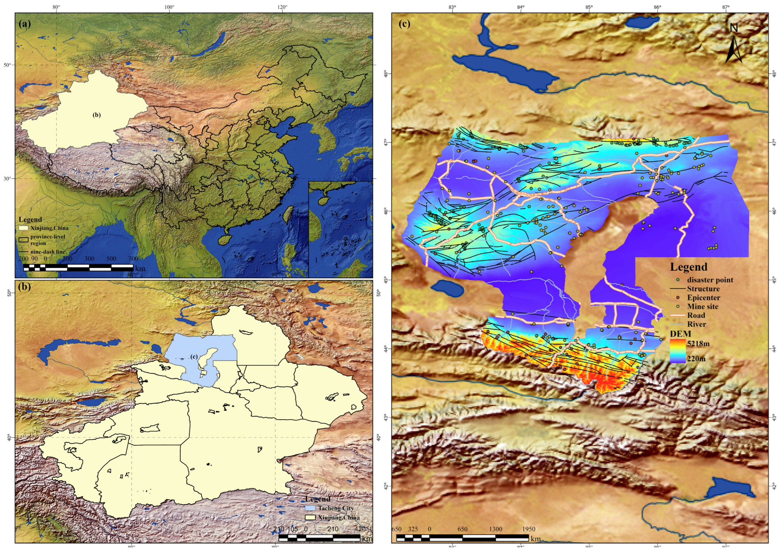
As shown in Figure 1, the Tacheng region is located in northwestern Xinjiang, China, between approximately 43°25′–47°15′N and 82°16′–87°21′E. It includes the western Junggar Mountains in the north and west, the northern Tianshan Mountains in the south, and the intervening Junggar Basin and intermontane depressions. The landscape comprises mountain ranges, basins, piedmont zones, and deeply incised river valleys. Geological hazards are concentrated mainly along river valleys, mountain roads, and piedmont margins, where fluvial incision and slope excavation have created numerous steep natural and engineered slopes.

The exposed stratigraphic succession ranges from the Ordovician to the Neogene and includes carbonate rocks, conglomerate, sandstone, siltstone, mudstone, shale, volcanic rocks, metamorphic rocks, and intrusive rocks [24]. Quaternary gravel, sandy gravel, fine sand, silt, and residual–colluvial deposits are widely distributed on mountain slopes, terraces, valley floors, and piedmont areas. The main failure-prone materials include loose Quaternary silt and gravelly soil, weak mudstone and shale, interbedded strong and weak clastic rocks, and intensely weathered or tectonically fractured bedrock. Most regional landslides are shallow soil slides developed within residual–colluvial cover or along the soil–bedrock contact, where contrasts in permeability and mechanical strength promote water accumulation and shear strength reduction.

Tectonically, northern and central Tacheng belong mainly to the western Junggar domain, whereas Wusu and Shawan in the south are influenced by the Junggar foreland and northern Tianshan tectonic systems [25]. Major strike–slip faults, including the East Tacheng and Tuoli faults, occur in western Junggar, and Late Quaternary activity has been documented along the Tuoli Fault. The northern Tianshan margin is characterized by Cenozoic folding, faulting, and crustal shortening [26]. Faults, joints, bedding discontinuities, and crushed zones reduce rock mass integrity, provide potential failure surfaces, and facilitate water infiltration, particularly where river erosion or road cutting removes slope support.

The region has a temperate arid to semi-arid climate, with precipitation strongly controlled by elevation and topographic exposure. Geological hazards occur mainly during spring snowmelt and the summer rainy season [27]. Rainfall and snowmelt infiltration increase soil moisture and pore water pressure in loose deposits, fractures, and weak soil–bedrock interfaces, thereby reducing effective stress and shear resistance [28]. Intense runoff can also erode and entrain loose slope and channel materials, promoting channelized debris flows [29]. Based on field investigations and historical records, as of June 2020, a total of 1260 geological hazard sites have been identified in the region, threatening 2172 people and assets valued at approximately 155 million CNY. Therefore, selecting this area as the study region for landslide susceptibility assessment and the investigation of landslide-triggering mechanisms is of significant scientific and practical value.

2.2. Dataset

2.2.1. Historical Landslides

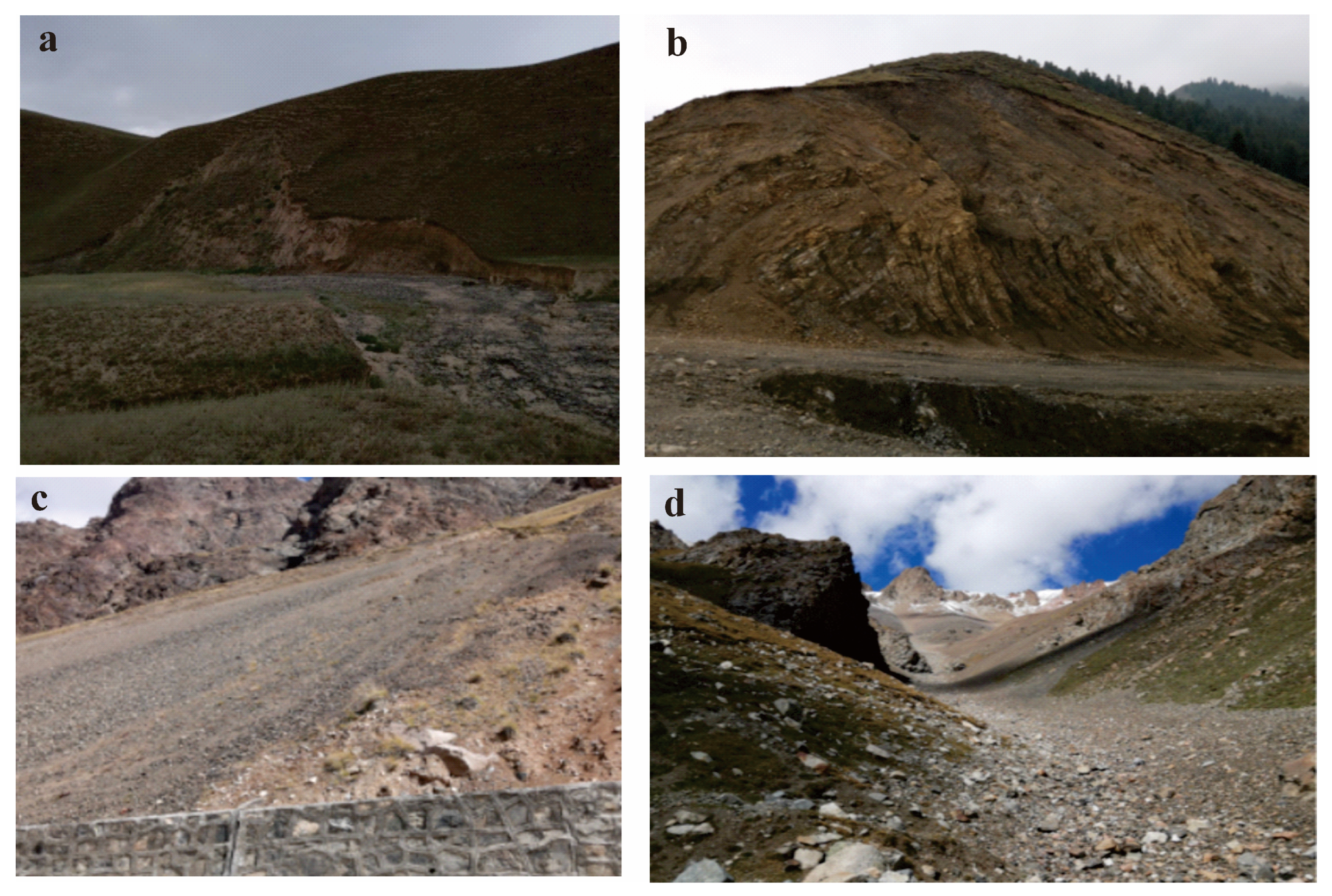
As of 2025, a total of 164 representative slope instability events were compiled from field investigations, historical records, and satellite image interpretation. The inventory includes slide-type landslides, channelized debris flows, and inventoried unstable slopes with evidence of incipient deformation. For attribute encoding, unstable slopes with clear evidence of incipient deformation were grouped into the landslide category. Consistent with the regional geological setting described in Section 2.1, the inventoried events are dominated by shallow failures in Quaternary residual–colluvial cover, with fewer failures occurring in weathered and fractured bedrock. Representative engineering–geological types are illustrated in Figure 2 and include: (a) shallow intra-layer soil slides; (b) soil–bedrock contact slides; (c) shallow rock slides controlled by bedding planes, joints, or other discontinuities; and (d) channelized debris flows [30]. In the broad geomorphological sense, landslides encompass several forms of gravity-driven mass movement, including flows, and debris flows are commonly classified as flow-type landslides [29]. Previous studies have therefore incorporated shallow landslides and debris flows into common landslide susceptibility frameworks [31,32]. Following this convention, slide-type landslides and debris flows were jointly incorporated into the unified susceptibility framework, while their differences in hazard type and associated attributes were explicitly retained through the tabular input.

The landslide inventory used in this study records landslide events as centroid locations. These centroid points were used to represent the occurrence locations of individual landslide events and to construct samples for landslide susceptibility modeling. To mitigate class imbalance, an equal number of non-landslide points were selected using a random sampling strategy. A 2 km buffer was established around each landslide centroid, and non-landslide points were sampled outside these buffers to reduce spatial autocorrelation and potential labeling ambiguity [33]. Therefore, the final sample dataset contained 328 samples, including 164 positive samples and 164 negative samples.

2.2.2. Rasterized Spatial Conditioning Factors

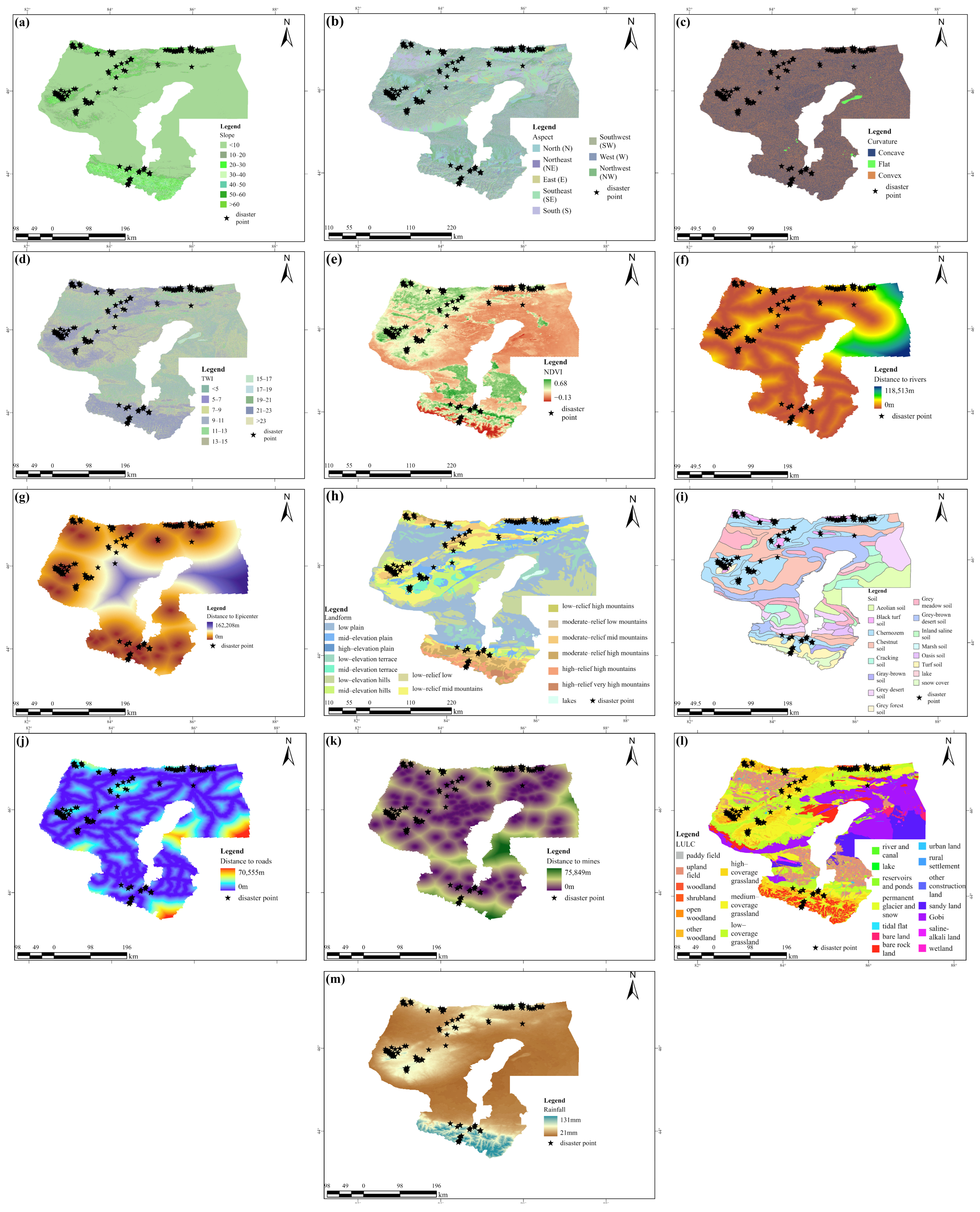
The performance of landslide susceptibility mapping (LSM) depends strongly on the selection of conditioning factors [34]. This study considers multiple types of conditioning factors, including topographic, land cover, geological, hydrological, climatic, and anthropogenic variables. Among these factors, elevation plays a key role in landslide initiation and spatial distribution [35]. Elevation data were obtained from the ALOS PALSAR digital elevation model (DEM). Slope, aspect, curvature, and the topographic wetness index (TWI) were derived from the DEM using ArcGIS Pro 3.0.2. Land use/land cover (LULC) data were extracted from Sentinel-2 imagery. Rainfall and NDVI data were obtained from the Tibetan Plateau Data Center. Geological factors include landform types and distances to roads, rivers, and mining sites. These factors were derived from geological maps using cumulative distance analysis. Distances to historical earthquake epicenters were calculated from seismic records provided by the National Earthquake Data Center [36]. Detailed information on all conditioning factors, data sources, and spatial resolutions is provided in

Table 1. Candidate conditioning factors initially considered in this study.

S.No	Variables	Sources	Resolution	Description
1	Slope, elevation, Aspect, Curvature, TWI	Digital elevation model	12.5 m	ALOS-PALSAR-DEM (https://search.asf.alaska.edu/)
2	LULC	Sentinel-2 imagery	10 m	https://www.impactobservatory.com/
3	Distance to roads Distance to rivers Distance to mines landform	Geological Map	/	Geological Survey of Tacheng
4	Rainfall, NDVI	TDPC	0.0083333°	https://www.tpdc.ac.cn/home
5	soil types	CERN	30 m	http://soilhub.cn/
6	distance to Epicenter	NEDC	/	https://data.earthquake.cn/

and Figure 3.

Topographic factors play a fundamental role in controlling landslide occurrence and spatial distribution. Elevation influences geomorphic evolution and the distribution of gravitational potential energy, which affects slope stability. Slope directly controls stress distribution and material accumulation on hillslopes [37]. Aspect regulates solar radiation conditions and surface moisture regimes, which in turn affect weathering intensity and slope stability [38]. Curvature reflects the spatial geometric characteristics of the terrain surface and describes the concave–convex features of slopes and their variation trends. Different curvature conditions influence surface runoff pathways, material transport processes, and local stress distribution, thus playing an important role in slope stability. In general, concave terrains tend to facilitate the convergence of water and loose materials, whereas convex terrains are more prone to erosion; both processes are closely associated with landslide initiation and development [39]. The topographic wetness index (TWI) integrates slope and upstream contributing area and is used to characterize areas susceptible to water accumulation and elevated pore water pressure [40].

Vegetation and surface characteristics also exert a significant influence on slope stability. The normalized difference vegetation index (NDVI) is used to characterize vegetation cover; vegetation can enhance slope stability by reinforcing soil through root systems and reducing surface erosion, thereby affecting landslide occurrence [41]. Land use/land cover (LULC) data reflect surface modifications caused by human activities such as deforestation, agricultural practices, and urban expansion, which can alter slope conditions and are closely related to landslide occurrence [42,43]. Soil type represents the mechanical and hydraulic properties of near-surface materials, including cohesion, permeability, and weathering susceptibility, and is therefore a key factor influencing slope stability [44]. In addition, geomorphological units (e.g., low-elevation plains, mid-altitude hills, and high-elevation mountains) integrate the combined effects of terrain relief, tectonic setting, and surface processes, providing important indicators for landslide development [45].

Hydrological and triggering factors play an important role in landslide occurrence. Rainfall is one of the main triggering factors of landslides, as prolonged or intense precipitation can increase soil moisture and lead to slope failure [35]. Distance to rivers reflects the impact of fluvial erosion on slope toes, and slopes located closer to rivers are more prone to instability [46]. Distance to historical earthquake epicenters represents the influence of seismic activity on slope stability. In addition, distances to roads and mining sites are used to characterize disturbances caused by human engineering activities, which often weaken slope stability and trigger landslides [47].

After comprehensively considering data availability and landslide formation mechanisms, multiple landslide conditioning factors were selected for modeling and analysis in this study. All factors were converted into raster format and resampled to a uniform spatial resolution of 30 m. Categorical variables, including geomorphological type, soil type, and land use/land cover (LULC), were classified according to established standards, while continuous variables were discretized based on expert knowledge and previous studies to optimize their value distributions. To ensure comparability among factors and to improve model convergence, all continuous variables were normalized using the min–max normalization method, scaling their values to the range of 0–1. This ensures the comparability of different factors in the modeling process while also accelerating model convergence and enhancing prediction stability and accuracy [48].

2.2.3. Landslide Attribute Data

In addition to raster-based conditioning factors, this study used tabular attribute information to enrich the model inputs. These attributes describe the basic characteristics of landslide and debris flow events. They provide complementary information that cannot be fully represented by raster variables alone. As shown in

Table 2. Landslide and debris flow attribute variables used in this study.

Variable	Description	Type	Example
Hazard Type	Type of geological hazard event recorded in the inventory	Categorical	Landslide, Debris flow
Triggering Factor	Primary external factor responsible for initiating the hazard event	Categorical	Rainfall, Earthquake, Human activity
Material Type	Dominant geological material involved in the mass movement	Categorical	Soil, Rock, Mixed
Hazard Magnitude	Estimated overall scale or intensity level of the hazard event	Ordinal	Small, Medium, Large
Activity Level	Current activity status of the hazard body	Ordinal	Active, Dormant, Stabilized

, the tabular dataset includes hazard type, triggering factor, material type, hazard magnitude, and activity level. These attributes describe the event type, possible triggering mechanism, material composition, overall scale, and activity state of each hazard event.

To enable quantitative analysis of the relationships between environmental conditions and landslide attributes, the recorded attributes were encoded according to their variable types. Hazard type, triggering factor, and material type were treated as nominal categorical variables and encoded using one-hot encoding. For example, hazard type was encoded as landslide = [1, 0] and debris flow = [0, 1]. Triggering factor was encoded as rainfall = [1, 0, 0], earthquake = [0, 1, 0], and human activity = [0, 0, 1]. Material type was encoded as soil = [1, 0, 0], rock = [0, 1, 0], and mixed = [0, 0, 1]. In contrast, hazard magnitude and activity level were treated as ordinal variables because they contain explicit ranking information. Hazard magnitude was encoded as small = 0, medium = 1, and large = 2, whereas activity level was encoded as stabilized = 0, dormant = 1, and active = 2. Representative attribute records and their corresponding encoded vectors are provided in

Table 3. Examples of landslide attribute records and encoded vectors.

Sample ID	Hazard Type	Trigger	Material	Magnitude	Activity	Encoded
001	Landslide	Rainfall	Soil	Medium	Active	[1,0; 1,0,0; 1,0,0; 1; 2]
002	Debris flow	Rainfall	Mixed	Medium	Active	[0,1; 1,0,0; 0,0,1; 1; 2]
003	Landslide	Human activity	Rock	Small	Dormant	[1,0; 0,0,1; 0,1,0; 0; 1]
004	Landslide	Earthquake	Rock	Large	Stabilized	[1,0; 0,1,0; 0,1,0; 2; 0]

. These encoded attributes were used only to quantify environmental–attribute associations and construct category-specific environmental prototypes; they were not directly supplied to the FiLM-U-Net. Instead, all samples were represented by the unified soft attribute-prior vectors described in Section 2.2.4.

2.2.4. Soft Attribute-Prior Estimation for Non-Landslide Samples

Event-specific landslide attributes, such as hazard type, triggering factor, material type, hazard magnitude, and activity level, are only available for inventoried landslide events. These attributes are unavailable for unknown regional pixels. Directly assigning null values, zeros, or fixed values to these fields may cause the model to distinguish landslide and non-landslide samples based on attribute availability. This can lead to information leakage and reduce the reliability of regional susceptibility mapping. To address this problem, this study developed an association-weighted soft attribute-prior estimation strategy.

To ensure a consistent tabular representation, recorded landslide attributes were used only to establish environmental–attribute relationships, while all samples and regional pixels were represented by uniformly estimated soft attribute priors.

First, a fixed-length environmental descriptor vector was extracted from each 512 × 512 raster patch. For the ten continuous factors, including slope, aspect, curvature, TWI, rainfall, NDVI, and distances to roads, rivers, mining sites, and earthquake epicenters, the mean, standard deviation, center-pixel value, minimum, and maximum were calculated, yielding 50 descriptors. For the categorical factors, including LULC, soil types, and landform, the proportion of valid pixels belonging to each class was calculated as

$$r_{i,k}={\displaystyle \frac{n_{i,k}}{N_i}}$$

(1)

where $n_{i,k}$ is the number of pixels assigned to class $k$ in patch $i$, and $N_i$ is the total number of valid pixels. All descriptors were concatenated into a vector of dimension $p=50+K_{\mathrm{L}\mathrm{U}\mathrm{L}\mathrm{C}}+K_{\mathrm{s}\mathrm{o}\mathrm{i}\mathrm{l}}+K_{\mathrm{l}\mathrm{a}\mathrm{n}\mathrm{d}\mathrm{f}\mathrm{o}\mathrm{r}\mathrm{m}},$ with NoData pixels excluded from the calculation of all statistics and class proportions.

The inventoried landslide samples in the training subset were then used to quantify the associations between environmental descriptors and recorded landslide attributes. For each nominal attribute category, a binary indicator was generated using one-hot encoding. Spearman’s rank correlation coefficient was calculated between each encoded attribute category and each environmental descriptor. The absolute correlation coefficients were normalized to obtain category-specific association weights:

$$w_{A,c,j}={\displaystyle \frac{∣{\rho }_{A,c,j}∣}{{\displaystyle {\sum }_{m=1}^p}∣{\rho }_{A,c,m}∣+ϵ}}$$

(2)

where ${\rho }_{A,c,j}$ denotes the Spearman correlation coefficient between category $c$ of attribute $A$ and environmental descriptor $j$, and $ϵ$ is a small constant used to avoid division by zero. Environmental descriptors that were more strongly associated with a particular attribute category therefore received greater weights in the subsequent similarity calculation.

An environmental prototype was subsequently constructed for each category or ordered level of every landslide attribute. Let ${\mathcal{I}}_{A,c}$ denote the set of training landslide samples belonging to category $c$ of attribute $A$. The prototype of the $j$-th environmental descriptor was defined as

$${\mu }_{A,c,j}={\displaystyle \frac{1}{\mid {\mathcal{I}}_{A,c}\mid }}\sum _{n\in {\mathcal{I}}_{A,c}}{z}_{n,j}$$

(3)

The prototype vector ${\mu }_{A,c}$ therefore represents the typical environmental conditions associated with category $c$ of attribute $A$. For every sample, irrespective of whether it was an inventoried landslide or a non-landslide sample, its environmental descriptor vector was compared with the prototypes of all categories within each landslide attribute. The association-weighted similarity score was calculated using a standardized weighted $L_1$ distance:

$$S_{i,A,c}=-{\displaystyle \sum _{j=1}^p}{w}_{A,c,j}{\displaystyle \frac{∣z_{i,j}-{\mu }_{A,c,j}∣}{{\sigma }_j+ϵ}}$$

(4)

where $S_{i,A,c}$ denotes the similarity between sample $i$ and category $c$ of attribute $A$, $w_{A,c,j}$ is the corresponding association weight, and ${\sigma }_j$ is the standard deviation of descriptor $j$ estimated from the training subset. The negative sign converts the weighted environmental distance into a similarity score, such that a closer match to a category prototype produces a higher score.

The category-specific similarity scores were then normalized within each attribute using a group-wise softmax function:

$$P\left(A=c\mid X_i\right)={\displaystyle \frac{\exp \left(S_{i,A,c}\right)}{{\displaystyle {\sum }_{k=1}^{K_A}}\exp \left(S_{i,A,k}\right)}}$$

(5)

where $K_A$ is the number of categories or ordered levels of attribute $A$. For example, when $A$ denotes the triggering factor, the softmax output represents the probabilities associated with rainfall, earthquake, and human activity.

For nominal attributes, including hazard type, triggering factor, and material type, the complete category probability vectors were retained as the soft attribute-prior representations. For ordinal attributes, including hazard magnitude and activity level, the category probabilities were converted into expected ordinal scores:

$${\widehat{o}}_{i,A}={\displaystyle \sum _{c=0}^{K_A-1}}c P\left(A=c\mid X_i\right)$$

(6)

This formulation preserves the ordering among attribute levels without assigning a deterministic category. Finally, the soft priors of all five attributes were concatenated in a fixed order:

$$a_i=\left[p_i^{\mathrm{h}\mathrm{a}\mathrm{z}\mathrm{a}\mathrm{r}\mathrm{d}},p_i^{\mathrm{t}\mathrm{r}\mathrm{i}\mathrm{g}\mathrm{g}\mathrm{e}\mathrm{r}},p_i^{\mathrm{m}\mathrm{a}\mathrm{t}\mathrm{e}\mathrm{r}\mathrm{i}\mathrm{a}\mathrm{l}},{\widehat{o}}_i^{\mathrm{m}\mathrm{a}\mathrm{g}\mathrm{n}\mathrm{i}\mathrm{t}\mathrm{u}\mathrm{d}\mathrm{e}},{\widehat{o}}_i^{\mathrm{a}\mathrm{c}\mathrm{t}\mathrm{i}\mathrm{v}\mathrm{i}\mathrm{t}\mathrm{y}}\right]$$

(7)

The five attribute priors were combined into a ten-dimensional vector, consisting of 2, 3, and 3 dimensions for the three nominal attributes and one dimension for each ordinal attribute. This vector was used as the tabular input to the FiLM-U-Net. To prevent information leakage, all descriptor standardization parameters, Spearman association weights, and environmental prototypes were estimated exclusively from the training data. During five-fold cross-validation, these quantities were fitted using only the training folds and then applied to the held-out validation fold. Soft attribute priors for the training samples were generated using an out-of-fold procedure so that the recorded attribute of a sample was not used to construct the rule that generated its own prior. For the final independent test evaluation, the association weights and prototypes were estimated using the complete development set and then applied to the independent test set. No validation or independent-test information was used during soft attribute-prior construction.

3. Method

3.1. U-Net

Convolutional neural networks (CNNs) take raw raster data as inputs. They extract hierarchical features through convolution operations, nonlinear activation functions, and downsampling. The learned features are then mapped to the target task through upsampling and reconstruction, which enables probabilistic prediction. Although many CNN architectures have been developed, most of them follow a similar structure, including an input layer, convolutional layers, pooling layers, and an output layer.

U-Net is a classical encoder–decoder convolutional neural network with a symmetric architecture. It consists of an encoder and a decoder. Skip connections are used to combine low-level spatial details with high-level semantic information. This design improves spatial localization accuracy and enhances the representation of multi-scale features. Unlike traditional CNNs, U-Net is designed for pixel-level classification tasks. The model predicts each pixel (raster cell) in the input image. As a result, it can generate continuous and high-resolution spatial prediction results for the study area [49].

In addition, U-Net is suitable for multi-source information fusion. The encoder can extract features from multi-channel input data. Skip connections combine original spatial information with high-level semantic features. This provides rich contextual and local detail information for the model. Therefore, U-Net is well suited for joint modeling of raster data and tabular data or multi-channel factor data. It enables efficient multimodal data fusion and improves the predictive performance of landslide susceptibility mapping [50].

3.2. FiLM

FiLM (Feature-wise Linear Modulation) is a conditional modulation mechanism designed to inject external information into convolutional neural networks, enabling multi-modal feature fusion [51]. Its core idea is to linearly scale and shift each channel of the convolutional feature map using a condition vector, allowing the feature representation to dynamically adapt according to the conditional information. Let the $c$-th channel of a convolutional feature map be ${ F}_c\in {\mathbb{R}}^{H\times W}$ and the condition vector be $z\in {\mathbb{R}}^d$. The FiLM modulation process can be expressed as:

$$\mathrm{F}\mathrm{i}lM\left(F_c\right)={\gamma }_c·F_c+{\beta }_c$$

(8)

where ${\gamma }_c$ and ${\beta }_c$ are generated from the condition vector:

$${\gamma }_c,{\beta }_c=f_c\left(z\right)$$

(9)

Here, $f_c(\cdot )$ is typically a small, fully connected network that maps the condition vector to modulation parameters for each channel.

In a U-Net with FiLM, the raster data are first processed by the encoder to extract features, while the soft attribute-prior vector is mapped to a condition vector via a tabular encoder. In the down-sampling modules or intermediate convolutional layers, FiLM modulates the feature maps channel-wise according to the condition vector. The modulated features are then concatenated with the corresponding encoder features through skip connections, fed into the decoder for up-sampling and reconstruction, and ultimately produce pixel-level predictions.

At the batch and spatial dimensions, FiLM can be written as:

$$F^{\prime }={\gamma }_c\odot F+\beta \left(c\right)$$

(10)

where $F\in {\mathbb{R}}^{B\times C\times H\times W}$, $\gamma (c),\beta (c)\in {\mathbb{R}}^{B\times C\times 1\times 1}$, and $\odot$ denotes channel-wise broadcasted multiplication. This mechanism not only achieves efficient fusion of raster features and tabular information while preserving spatial structure but also enhances the model’s adaptability to multi-modal inputs.

3.3. FiLM-U-Net

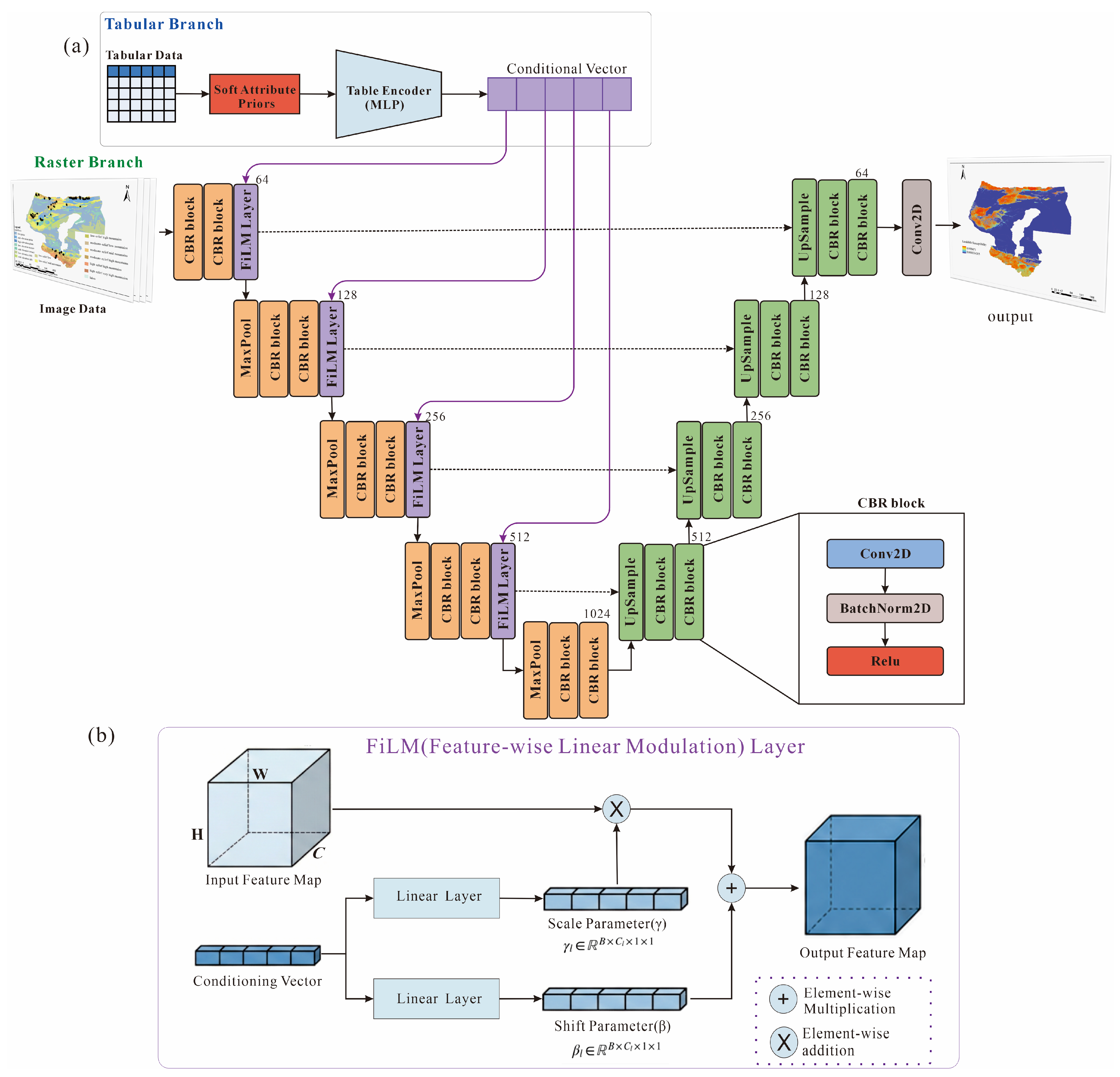
To integrate rasterized spatial conditioning factors with landslide-related tabular attributes, this study develops a multi-stage FiLM-conditioned U-Net architecture, as illustrated in Figure 4. The proposed model consists of two parallel input branches: a raster branch for spatial feature extraction and a tabular branch for conditional-information encoding.

Let $X\in {\mathbb{R}}^{B\times C_x\times H\times W}$ denote a multi-channel raster patch containing the retained landslide conditioning factors, and let $a\in {\mathbb{R}}^{B\times d_a}$ denote the soft attribute-prior vector. The raster branch adopts a U-Net encoder–decoder architecture. The encoder progressively extracts multi-scale spatial features through convolutional blocks and max-pooling operations, while the decoder gradually reconstructs spatial details through up-sampling and skip connections. In parallel, the soft attribute-prior vector is processed by an independent tabular encoder. The tabular attributes include hazard type, triggering factor, material type, hazard magnitude, and activity level. The tabular encoder consists of three fully connected layers with output dimensions of 64, 128, and 64, respectively. Each fully connected layer is followed by batch normalization and a ReLU activation function. The final output is a 64-dimensional condition vector:

$$z\in {\mathbb{R}}^{B\times 64}$$

(11)

Image–tabular fusion is performed at four encoder stages using FiLM modules, with feature-channel dimensions of 64, 128, 256, and 512. At stage $l$, the convolutional block outputs a feature tensor $F_l$.

$$F_l\in {\mathbb{R}}^{B\times C_l\times H_l\times W_l},C_l\in \left\{64, 128, 256, 512\right\}$$

(12)

For each encoder stage, two stage-specific linear mappings transform the shared condition vector into scaling and shifting parameters:

$${\gamma }_l=h_l^{\gamma }\left(z\right),{\beta }_l=h_l^{\beta }\left(z\right)$$

(13)

where ${\gamma }_l,{\beta }_l\in {\mathbb{R}}^{B\times C_l}$, with one scaling and one shifting parameter generated for each feature channel. They are reshaped to ${\mathbb{R}}^{B\times C_l\times 1\times 1}$ and applied uniformly across all spatial locations of the corresponding channels. The encoder features are then modulated as follows.

$${\tilde{F}}_l={\gamma }_l\odot F_l+{\beta }_l$$

(14)

Although the same 64-dimensional condition vector is supplied to all four FiLM modules, each encoder stage has independent mappings $h_l^{\gamma }$ and $h_l^{\beta }$. Therefore, the tabular information can modulate feature channels differently at different spatial resolutions. At each encoder stage, FiLM modulation is applied after the convolutional blocks and before the feature tensor is transferred to the next down-sampling stage. The FiLM-modulated feature ${\tilde{F}}_l$ is also passed to the corresponding decoder stage through the skip connection. FiLM modules are applied at the four encoder stages, while no additional modulation is performed at the 1024-channel bottleneck.

During decoding, the lower-resolution features are progressively up-sampled. At each decoder stage, the up-sampled decoder feature is concatenated with the corresponding FiLM-modulated encoder feature. The combined feature is then processed by convolution–batch-normalization–ReLU blocks. This design preserves fine spatial information while transferring condition-aware semantic features from the encoder to the decoder. Finally, a $1\times 1$ convolution maps the reconstructed feature tensor to pixel-wise landslide susceptibility probabilities, producing a continuous susceptibility map.

The proposed strategy differs from conventional feature concatenation and late fusion. In concatenation-based fusion, the tabular vector is first expanded and concatenated with the image features, and subsequent convolutional layers learn the interactions between them. In contrast, FiLM transforms the tabular condition vector into channel-wise scaling and shifting parameters and directly modulates the image features at the encoder stages. This approach not only avoids the increase in feature channels caused by concatenation but also enables the model to selectively enhance or suppress image feature channels according to the tabular attributes. Moreover, by applying modulation at multiple encoder stages, the tabular information can guide multi-scale feature extraction throughout the network rather than contributing only near the output stage.

The soft attribute prior provides sample-specific contextual information for FiLM modulation. The tabular encoder first transforms the prior into a shared condition vector, which is further mapped to stage-specific scaling and shifting parameters for multi-scale feature modulation. During training, the spatial prediction loss optimizes the tabular encoder, FiLM mappings, and U-Net, allowing the model to learn how the prior information should be utilized at different feature levels. In this way, the soft prior supplies environmentally derived semantic cues, while FiLM translates these cues into task-adaptive spatial feature modulation.

The principal hyperparameters were selected through grid search using only the model development set. Candidate learning rates of {1 × 10⁻⁵, 5 × 10⁻⁵, 1 × 10⁻⁴, 5 × 10⁻⁴}, batch sizes of {4, 8, 16}, early-stopping patience values of {10, 20, 30}, and condition-vector dimensions of {32, 64, 128} were evaluated. The mean AUC across the stratified five-fold cross-validation was used as the selection criterion. The final configuration consisted of a learning rate of 1 × 10⁻⁴, a batch size of 16, a patience value of 20, and a 64-dimensional condition vector. The independent test set was not used during hyperparameter selection.

4. Experiments and Results

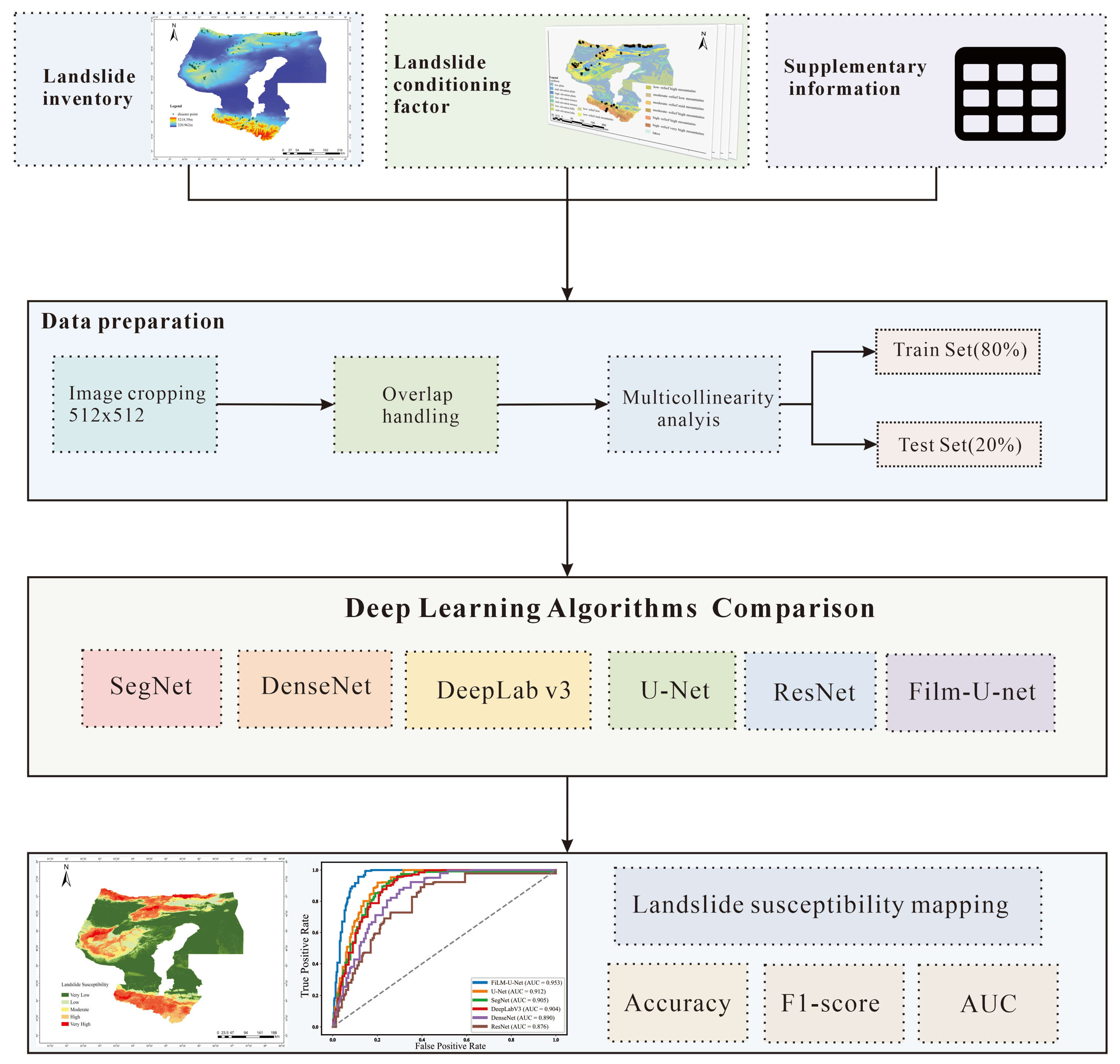
In this study, landslide inventory data, landslide conditioning factors, and relevant supplementary tabular data were collected to construct a comprehensive landslide dataset. Subsequently, the dataset was cropped and overlaid, and the potential collinearity among the landslide conditioning factors was examined. The final dataset was first divided into a model development set and an independent test set using a stratified 80/20 split. Stratified five-fold cross-validation was then performed on the development set for model training and validation, while the independent test set was used only for final performance evaluation. Finally, the complete raster dataset of the study area was input into the trained models to estimate landslide susceptibility probabilities across the entire region. The overall workflow of this study is illustrated in Figure 5.

4.1. Data Preparation

In the study area, landslide samples were constructed using the inventoried landslide points as patch centers. An equal number of non-landslide points were uniformly sampled at 1 km intervals outside a 2 km buffer surrounding each landslide location. The corresponding conditioning-factor layers were then cropped into 512 × 512-pixel patches to form the basic sample units.

Because the inventory records landslide centroids rather than complete source, transport, and depositional boundaries, a neighborhood radius was required for pixel-level label construction. Regional studies have characterized the spatial distribution and environmental controls of landslides across Xinjiang [27]. More detailed investigations show that most loess landslides in the Yili Valley have lengths and widths of 10–300 m [52], while maximum runout distances of 12 landslides in the Piliqinghe Basin range from approximately 47 to 375 m [53]. However, highly mobile events may travel much farther; for example, the flow-like Areletuobie landslide travelled approximately 1.8 km along a valley [54]. InSAR-, UAV-, LiDAR-, and field-based studies further indicate that landslide boundaries are strongly controlled by slope morphology and deformation patterns [55]. These findings demonstrate that landslide extent in Xinjiang varies with failure type, mobility, and terrain conditions, and cannot be represented by a universal physical radius [52,53,54,55].

Because measured landslide dimensions and runout distances cannot be directly converted into a circular radius around a centroid, the literature was used to define a plausible range of candidate neighborhood scales. A radius of 300 m represented a relatively conservative labeling scheme, whereas 800 m represented a more expansive scheme that was more likely to cross topographic boundaries. The 500 m radius was therefore adopted as an intermediate baseline and evaluated through sensitivity experiments using 300, 500, and 800 m radii. Pixels within 500 m of each landslide centroid were assigned positive labels, whereas pixels outside this radius within the same patch were assigned negative labels. For spatially overlapping samples, only one sample was retained, and overlapping areas in the remaining samples were excluded during training using a masking mechanism. The conditioning factors were subsequently examined for multicollinearity and normalized before model input.

The final dataset was divided using a stratified 80/20 split. The development set contained 262 samples, including 131 positive and 131 negative samples, while the independent test set contained 66 samples, including 33 positive and 33 negative samples. Stratified five-fold cross-validation was further performed on the development set, with the class ratio preserved in each fold. Model performance was reported as the mean and standard deviation across the five folds.

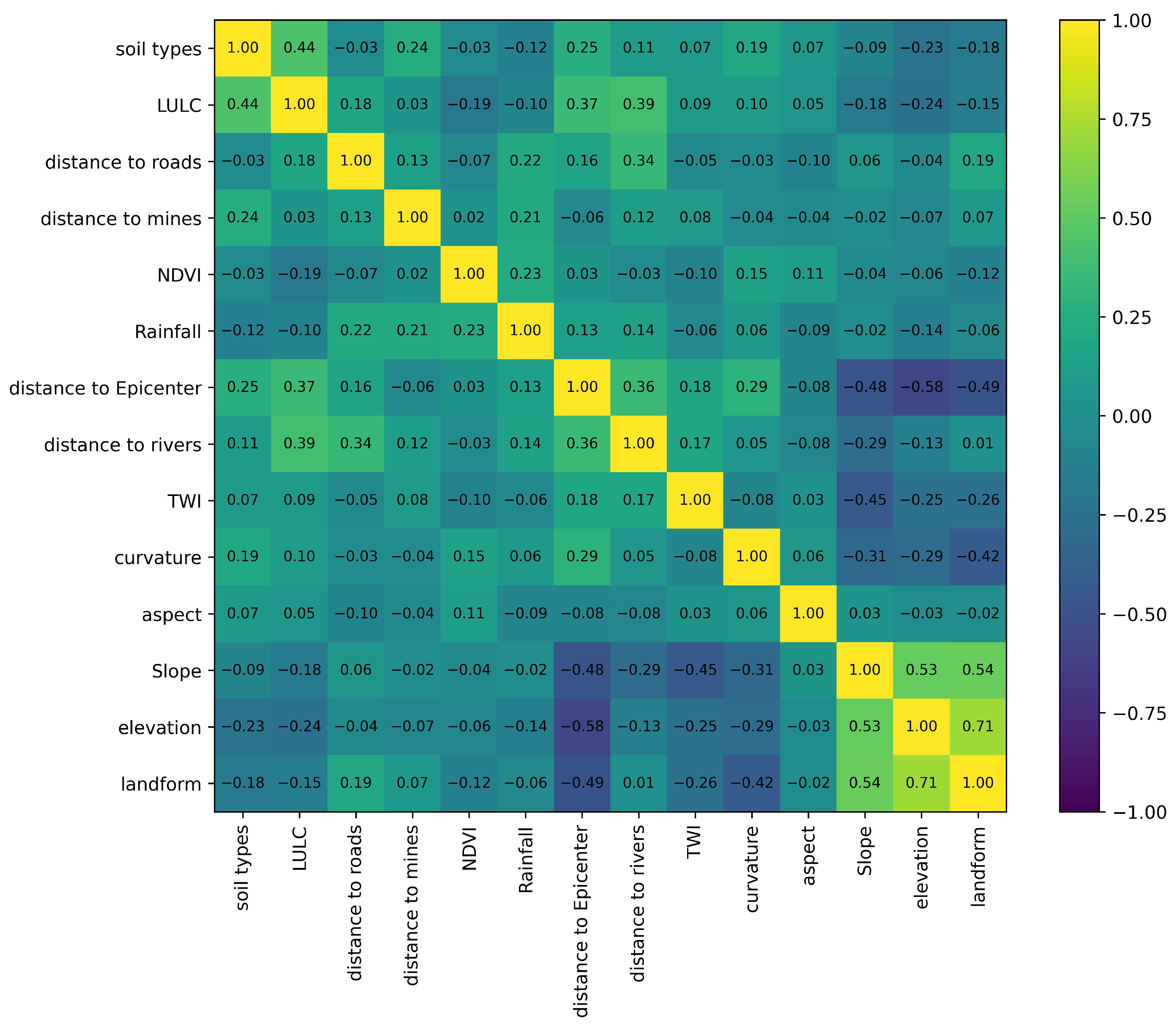
Previous studies have shown that, in landslide susceptibility mapping, highly correlated landslide conditioning factors may introduce redundant information, increase model complexity, and reduce the stability of variable-importance estimates [56,57]. Therefore, before model development, Spearman’s rank correlation coefficient was used to identify and screen highly correlated factors. Landslide occurrence is often influenced by threshold effects, factor interactions, geological complexity, and cumulative effects, resulting in relationships with conditioning factors that are frequently nonlinear and difficult to characterize accurately using simple linear models. As a rank-based and non-parametric measure, Spearman’s correlation coefficient can characterize monotonic relationships that are not necessarily linear, making it more appropriate for landslide susceptibility assessment than Pearson’s correlation coefficient, which primarily measures linear associations [27,58]. Following previous landslide susceptibility studies, an absolute Spearman correlation coefficient of $\mid {\rho }_s\mid >0.60$ was used to identify strong pairwise associations and potential factor redundancy [59,60]. As shown in Figure 6, elevation was removed because of its strong correlation with landform (${\rho }_s=0.71$).

4.2. Model Evaluation

Model performance was evaluated using a stratified five-fold cross-validation strategy combined with an independent test set. As described in Section 3.1, the final dataset contained 328 samples, including 164 positive samples and 164 negative samples. A stratified 80/20 split was first applied to divide the dataset into a model development set and an independent test set. The development set contained 262 samples, including 131 positive samples and 131 negative samples, whereas the independent test set contained 66 samples, including 33 positive samples and 33 negative samples. Stratified five-fold cross-validation was then performed on the development set. In each fold, four-fifths of the development samples were used for model training, and the remaining one-fifth was used for validation. The positive-to-negative sample ratio was preserved in each fold. Accuracy, F1-score, and AUC were calculated on the held-out validation fold, and the cross-validation results were reported as the mean and standard deviation across the five folds. After cross-validation, each model was retrained using the full development set and evaluated on the independent test set. The independent test set was not used during model training, hyperparameter tuning, or cross-validation. To avoid information leakage, all preprocessing operations that required statistical estimation, including normalization parameters and soft attribute-prior prototypes, were fitted only on the training subset of each fold and then applied to the corresponding validation subset. For the final independent test evaluation, these parameters were fitted using the full development set and applied to the independent test set.

Model performance was comprehensively evaluated using Accuracy, F1-score, and receiver operating characteristic (ROC) curves. In Equations (15) and (16), TP, TN, FP, and FN denote true positives, true negatives, false positives, and false negatives, respectively, and all evaluation metrics were derived from the confusion matrix. In addition, the ROC curves and the corresponding areas under the curve (AUCs) were calculated to further quantify the classification performance [61].

$$Accuracy={\displaystyle \frac{TP+TN}{TP+TN+FP+FN}}, F1-Score={\displaystyle \frac{2\times TP}{2\times TP+FP+FN}}$$

(15)

$$\mathrm{F}\mathrm{N}\mathrm{R}={\displaystyle \frac{FN}{FN+TP}}, \mathrm{F}\mathrm{D}\mathrm{R}={\displaystyle \frac{FP}{FP+TP}}, FPR={\displaystyle \frac{FP}{FP+TN}}$$

(16)

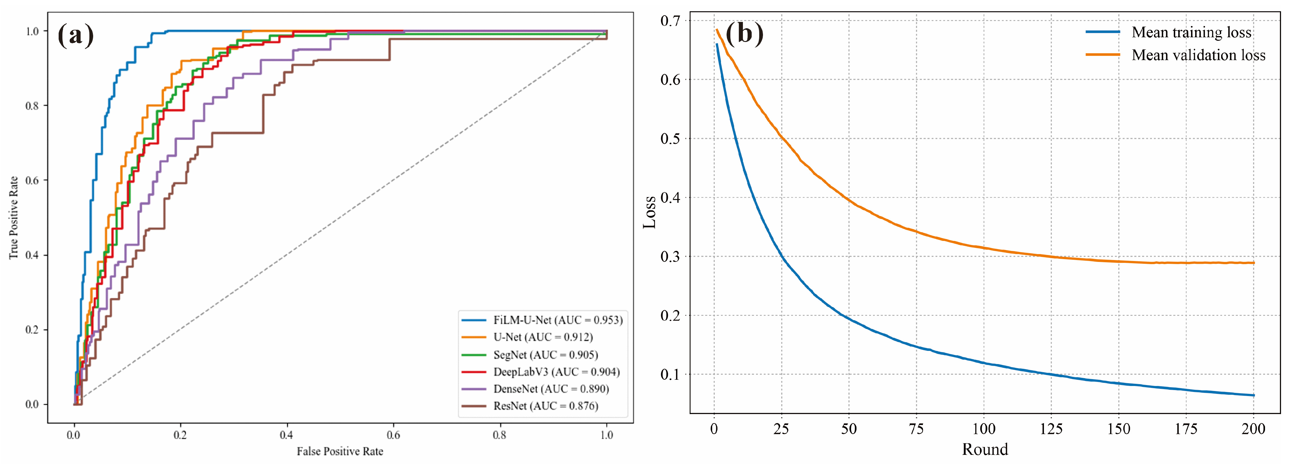
As shown in

Table 4. Performance comparison of different models based on five-fold cross-validation and independent testing.

Model	Five-Fold Cross-Validation			Independent Test Dataset
	Accuracy	F1-Score	AUC	Accuracy	F1-Score	AUC	FPR	FNR	FDR
FiLM-U-Net	91.84 $\pm$ 0.71	91.52 $\pm 0.76$	0.968 $\pm 0.005$	89.73	89.41	0.953	7.25	13.29	7.71
U-Net	89.26 $\pm$ 0.84	88.94 $\pm$ 0.88	0.934 $\pm 0.006$	87.58	87.12	0.912	8.85	15.99	9.53
SegNet	88.63 $\pm$ 1.12	88.17 $\pm 1.16$	0.928 $\pm 0.008$	86.92	86.45	0.905	9.61	16.55	10.33
DeepLab v3	87.74 $\pm$ 1.57	87.26 $\pm 1.61$	0.918 $\pm 0.011$	85.96	85.41	0.904	10.27	17.81	11.11
DenseNet	86.82 $\pm$ 1.49	86.31 $\pm 1.52$	0.900 $\pm 0.010$	84.78	84.21	0.890	11.61	18.83	12.51
ResNet	85.31 $\pm$ 0.95	84.88 $\pm 0.98$	0.892 $\pm$ 0.007	83.47	82.91	0.876	13.25	19.81	14.18
Late-Fusion U-Net	89.74 $\pm$ 0.82	89.31 $\pm$ 0.86	0.943 $\pm$ 0.006	87.84	87.42	0.926	8.82	15.5	9.45

Values under five-fold cross-validation are reported as the mean ± standard deviation calculated across the five held-out validation folds of the development set. Independent-test-set results were obtained after retraining each model on the complete development set.

, all models exhibit satisfactory classification performance in both the five-fold cross-validation and the independent test set. Among them, FiLM-U-Net achieved the best performance on the independent test set, with an accuracy of 89.73%, an F1-score of 89.41%, and an AUC of 0.953. It also obtained the lowest FPR, FNR, and FDR values of 7.25%, 13.29%, and 7.71%, respectively, indicating fewer false alarms and missed landslide predictions. Late-Fusion U-Net achieved the second-best performance among the tested models, followed by U-Net.

The remaining models show slightly lower but still competitive performance. SegNet and DeepLab v3 achieve test accuracies of 86.92% and 85.96%, with F1-scores of 86.45% and 85.41%, respectively, and AUC values of 0.905 and 0.904. DenseNet and ResNet obtain comparatively lower results, with test accuracies of 84.78% and 83.47%, and F1-scores of 84.21% and 82.91%, respectively.

Table 4 also reports the mean and standard deviation of the evaluation metrics obtained across the five held-out validation folds. The independent-test results were generally consistent with the cross-validation results, indicating stable predictive performance and reasonable generalization ability.

Furthermore, Table 4 and Figure 7a present the ROC curves and the corresponding AUC values for all models. Most models achieve test AUC values close to or higher than 0.90, demonstrating strong discriminative ability for landslide susceptibility prediction in the study area. In particular, the proposed FiLM-U-Net model achieves the highest AUC value, further confirming its superior capability in capturing the complex relationships between environmental factors and landslide occurrence. In addition, the mean training and validation loss curves in Figure 7b decreased steadily and remained close to each other, indicating stable convergence.

To evaluate the effects of the tabular attribute input and the FiLM modulation mechanism, we conducted an ablation analysis using three models: U-Net, Late-Fusion U-Net, and FiLM-U-Net. The U-Net model used only raster-based conditioning factors. The Late-Fusion U-Net added the soft attribute-prior vector at a late fusion stage. The FiLM-U-Net used the same attribute-prior vector for FiLM-based feature modulation. As shown in Table 4, the results show that Late-Fusion U-Net performed slightly better than U-Net. The test AUC increased from 0.912 to 0.926. This result indicates that the tabular attribute-prior vector provides useful supplementary information. Late-Fusion U-Net improved the test AUC from 0.912 to 0.926, indicating that the soft attribute-prior vector provides complementary information. FiLM-U-Net further increased the test AUC to 0.953 and reduced the FPR, FNR, and FDR to 7.25%, 13.29%, and 7.71%, respectively, suggesting that introducing the same soft prior during multi-scale spatial feature extraction is more effective than incorporating it only at the late-fusion stage. These results demonstrate the complementary roles of the two components: the soft prior provides sample-specific environmental and hazard-related context, while FiLM translates this context into stage-specific channel modulation, enabling more effective condition-aware feature learning.

The computational efficiency of all evaluated models was measured under the same hardware and software environment. All experiments were implemented using Python 3.10 and PyTorch 2.8.0 with CUDA 12.8 and executed on a workstation equipped with an NVIDIA GeForce RTX 5060 GPU. As shown in

Table 5. Computational efficiency comparison of the evaluated models.

Model	Parameters (M)	Total Training Time (Min/Epoch)	Inference Time (ms/Patch)
FiLM-U-Net	31.186	3.884	2447.59
U-Net	31.043	2.811	1958.79
SegNet	29.441	2.418	1544.15
DeepLab v3	39.665	3.843	1205.15
DenseNet	22.299	3.649	711.55
ResNet	40.950	3.124	680.71

, FiLM-U-Net contained 31.186 million trainable parameters, which was only 0.143 million more than the standard U-Net, corresponding to an increase of approximately 0.46%. This indicates that the tabular encoder and multi-stage FiLM modules introduced only a limited parameter overhead. Overall, the proposed model achieves a reasonable trade-off between predictive accuracy and computational efficiency.

4.3. Robustness and Generalization Evaluation

To further assess the effectiveness, spatial generalization ability, and robustness of the proposed framework, this study conducted an independent regional validation experiment, and buffer-radius sensitivity tests with 300 m, 500 m, and 800 m labeling radii.

4.3.1. Sensitivity Analysis of the Landslide-Label Radius

To evaluate the effect of the binary-label construction strategy, we tested three buffer-radius settings: 300 m, 500 m, and 800 m. The 300 m radius represents a conservative labeling scheme. In this setting, only pixels close to the landslide centroid were labeled as positive. The 500 m radius was used as the baseline setting in the main experiment. The 800 m radius represents a more relaxed labeling scheme. It covers a larger area around each landslide centroid, but it may also introduce more label uncertainty. In this experiment, only the label-generation radius was changed. The landslide sample locations, non-landslide sample selection strategy, conditioning factors, model architecture, hyperparameters, and train–test split procedure were kept the same. The results are shown in

Table 6. Performance comparison of FiLM-U-Net under different buffer-radius settings.

Extent	Five-Fold Cross-Validation			Independent Test Dataset
	Accuracy	F1-Score	AUC	Accuracy	F1-Score	AUC	FPR	FNR	FDR
300 m	90.76 $\pm$ 0.84	90.31 $\pm$ 0.88	0.958 $\pm$ 0.006	88.05	87.80	0.940	9.90	14.00	10.32
500 m	91.84 $\pm$ 0.71	91.52 $\pm 0.76$	0.968 $\pm 0.005$	89.73	89.41	0.953	7.25	13.29	7.71
800 m	91.11 $\pm$ 1.03	90.54 $\pm$ 1.07	0.956 $\pm$ 0.008	85.64	85.18	0.936	11.26	17.46	12.00

. Overall, FiLM-U-Net achieved high AUC values under all three buffer-radius settings. The 500 m setting achieved the best performance. It obtained a test accuracy of 89.73%, an F1-score of 89.41%, and an AUC of 0.953, together with the lowest FPR, FNR, and FDR values of 7.25%, 13.29%, and 7.71%, respectively. Under the 300 m setting, the test accuracy, F1-score, and AUC were 88.05%, 87.80%, and 0.940, respectively, with corresponding FPR, FNR, and FDR values of 9.90%, 14.00%, and 10.32%. Under the 800 m setting, these values were 85.64%, 85.18%, and 0.936, with corresponding FPR, FNR, and FDR values of 11.26%, 17.46%, and 12.00%, respectively. Compared with the 500 m baseline, the largest decrease in test AUC was 0.017. This indicates that the model maintained relatively stable discriminative ability under different buffer-radius settings. However, the 800 m setting showed a clearer decrease in accuracy and F1-score, together with higher omission and commission errors. This may be because the larger buffer introduced more uncertain positive labels around landslide centroids. Therefore, the 500 m radius provides a reasonable balance between conservative labeling and excessive expansion of positive labels. It was selected as the baseline label generation radius for the main experiment.

However, the 800 m setting showed a clearer decrease in accuracy and F1-score, together with higher omission and commission errors. As shown in

Table 7. Radial variations in slope and landform characteristics around hazard points.

Radial Zone	Mean Slope (°)	Pixels with Slope < 15° (%)	Low-Relief Landforms (%)	Pixels with a Landform Type Different from the Centroid (%)
0–300 m	13.45	61.77	48.97	4.70
300–500 m	14.60	55.61	49.48	8.18
500–800 m	15.77	55.05	51.00	11.45

, spatial examination of the additional positive pixels within the 500–800 m annulus showed a mean slope of 14.77°, with 55.05% of the pixels located on slopes below 15° and 51.00% occurring in low-relief landform classes. More importantly, 11.45% of the pixels had a landform type different from that at the hazard-point centroid, compared with 4.70% in the 0–300 m zone and 8.18% in the 300–500 m zone. Thus, although the outer annulus was not uniformly flatter than the inner zones, it showed greater geomorphological heterogeneity. Because a circular buffer does not conform to actual topographic boundaries, expanding the radius to 800 m is more likely to cross valley floors, ridgelines, or adjacent hillslopes and assign positive labels to environmentally dissimilar pixels. These pixels reduce the environmental consistency of the positive class, increase commission errors in surrounding non-landslide terrain, and weaken the model’s ability to distinguish the central landslide-affected area. Therefore, the 500 m radius provides a more reasonable balance between overly conservative labeling and excessive spatial expansion.

4.3.2. Spatially Independent Validation

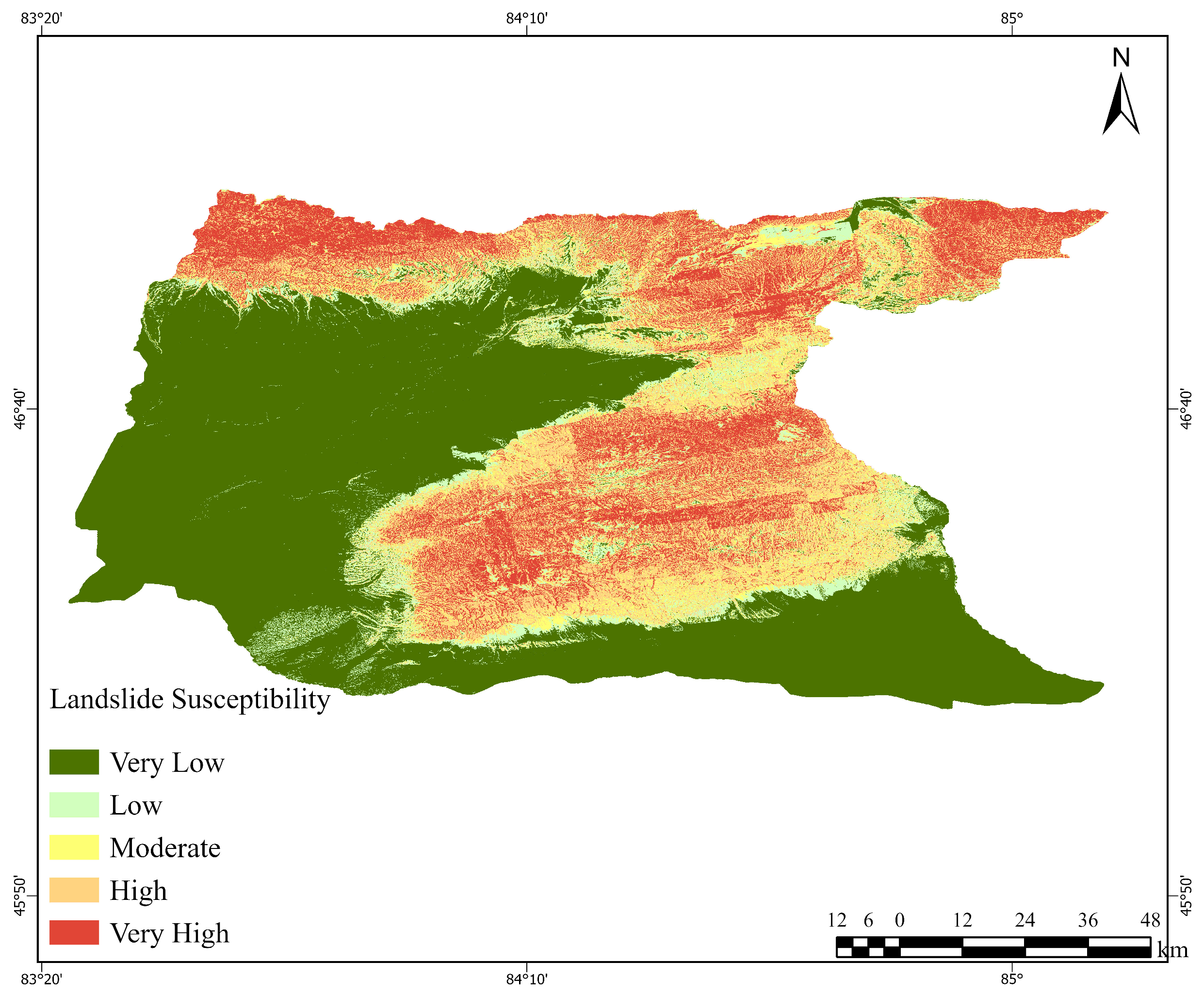
In addition to the stratified random train–test split and five-fold cross-validation, this study further conducted an administrative hold-out validation experiment to evaluate the spatial generalization ability of the proposed model. Random sample splitting may assign nearby samples with similar environmental conditions to both the training and testing subsets, which can lead to an optimistic estimation of model performance. Therefore, Emin County in Tacheng Prefecture was selected as an independent test area, while the remaining parts of the study area were used for model training and validation. In this experiment, the held-out administrative region was not involved in model training, hyperparameter selection, normalization parameter estimation, or soft attribute-prior construction. The quantitative results are summarized in

Table 8. Spatially independent validation results in Emin County.

Zone	Five-Fold Cross-Validation			Independent Test Dataset
	Accuracy	F1-Score	AUC	Accuracy	F1-Score	AUC
Emin County	90.28 $\pm$ 1.93	89.84 $\pm$ 1.97	0.951 $\pm$ 0.014	86.64	86.18	0.921

, and the landslide susceptibility map of Emin County is shown in Figure 8. The proposed FiLM-U-Net achieved an accuracy of 86.64%, an F1-score of 86.18%, and an AUC of 0.921 in Emin County. Although these values were slightly lower than those obtained from the random test set, the model still maintained acceptable predictive performance under spatially independent validation. As shown in Figure 8, the predicted high- and very high-susceptibility areas were mainly distributed in the central and northern parts of Emin County, while low-susceptibility areas were mainly concentrated in the southern and southwestern parts. The high-susceptibility zones generally correspond to areas with stronger terrain variation, more developed surface dissection, and potential influences from hydrological or human disturbance factors. These results indicate that the model learned relationships with a certain degree of transferability between landslide occurrence and conditioning factors.

4.4. Landslide Susceptibility Mapping

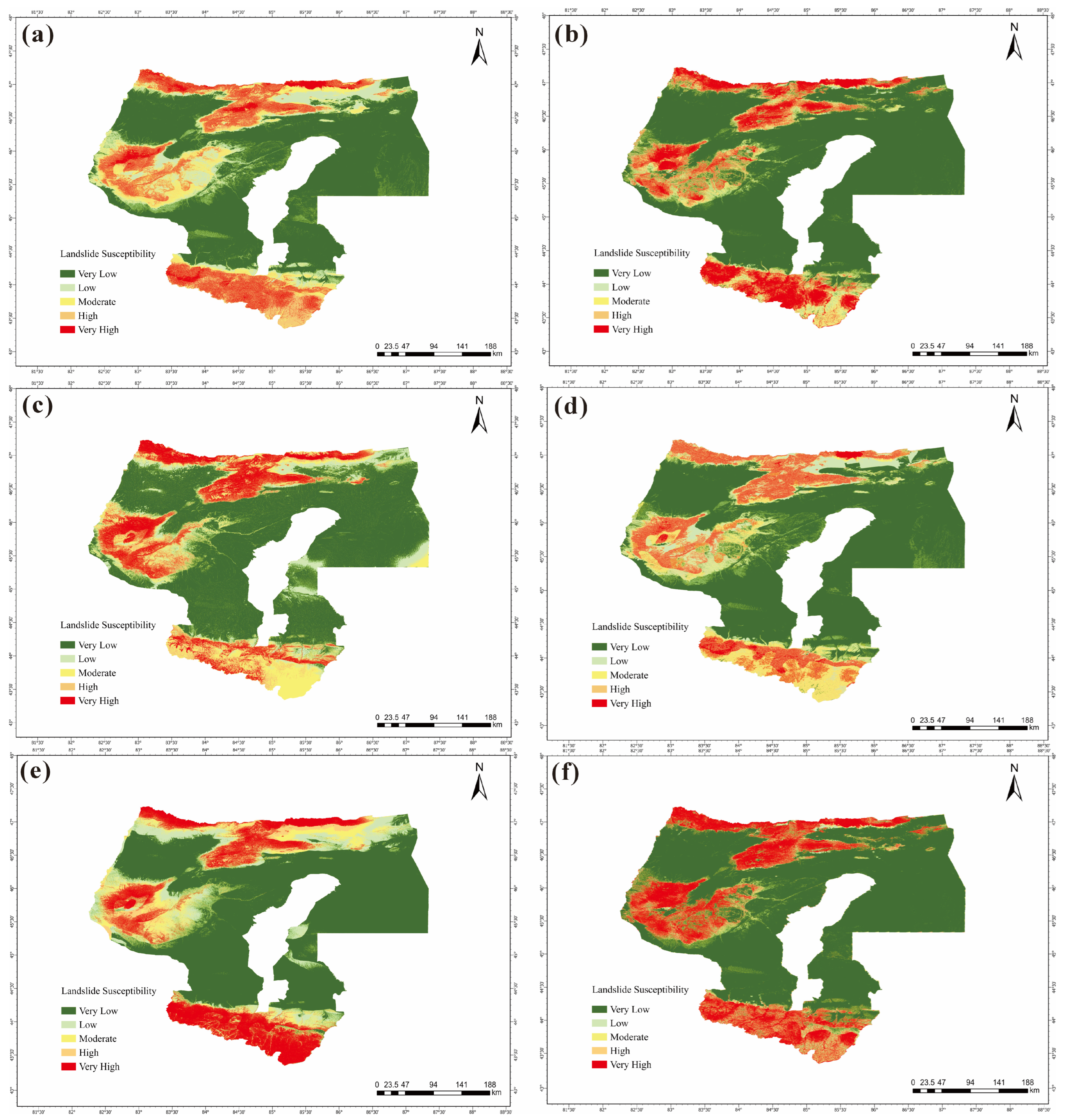
After inputting the complete dataset of the study area into the trained models, landslide susceptibility maps (LSMs) were generated using the FiLM-U-Net, U-Net, SegNet, DeepLab v3, DenseNet, and ResNet models, as shown in Figure 9. Overall, the spatial patterns of landslide susceptibility predicted by the different models are highly consistent. All models indicate that areas with high landslide susceptibility are mainly concentrated in the western, southern, and northern marginal zones of the study area, whereas the central and eastern regions are dominated by very low and low susceptibility levels.

By combining geospatial data with field investigation results, it can be observed that the southern and western parts of the study area exhibit high landslide susceptibility under the combined influence of multiple unfavorable conditioning factors. These areas show adverse combinations of terrain relief, slope conditions, river erosion effects, fault development, and disturbances from human engineering activities. In addition, rainfall conditions and land cover types in these areas also correspond well with the high-susceptibility zones. The spatial distribution of landslides is therefore controlled by the combined effects of topographic, geological, hydrological, climatic, and anthropogenic factors. Although some differences exist among models in the detailed boundaries and local patterns of high-susceptibility areas, the overall locations and spatial distribution of high-value zones remain highly consistent across models.

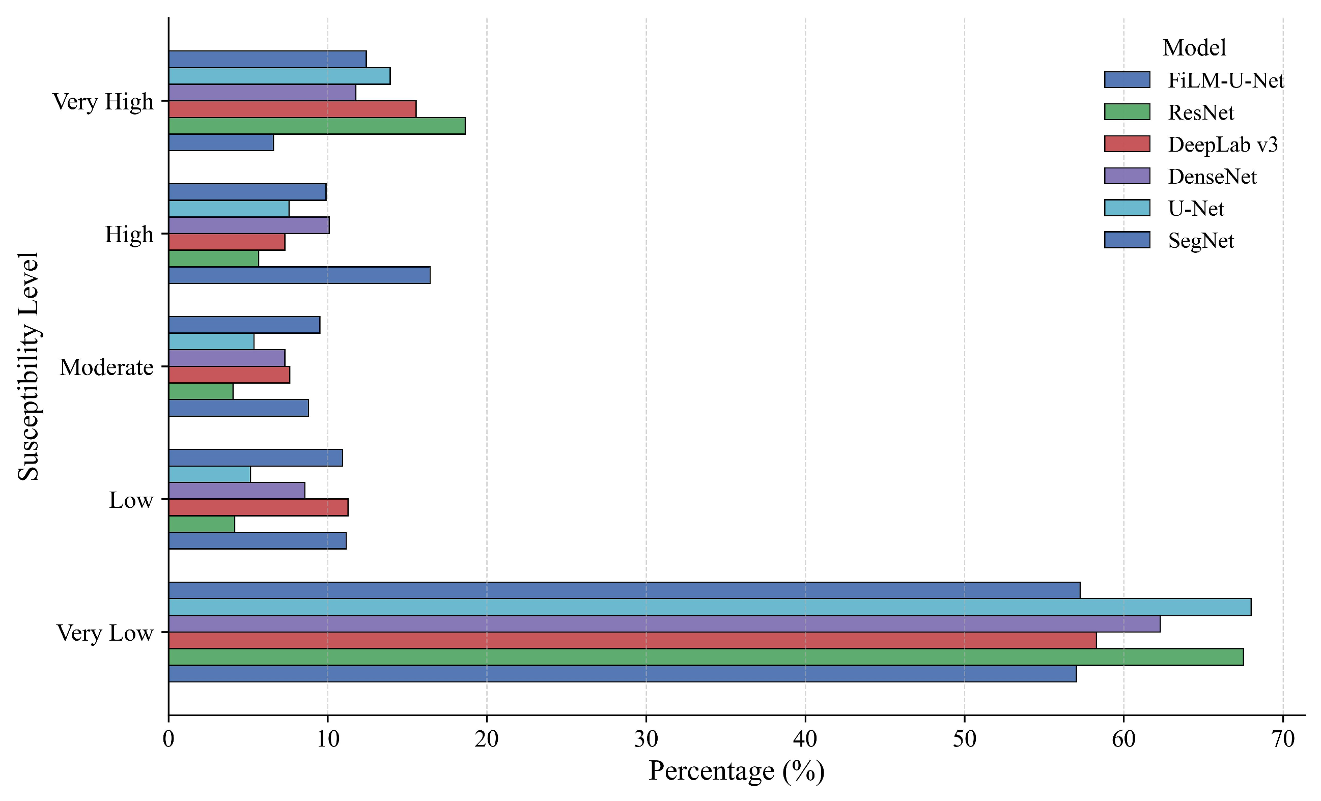
Figure 10 presents the area statistics of the five susceptibility classes for each model derived from the Natural Breaks classification. The results show that the very low susceptibility class occupies the largest proportion of the study area for all models, exceeding 55%. This indicates that the overall landslide susceptibility of the study area is relatively low, and landslide risk is mainly concentrated in localized areas. The low and moderate susceptibility classes account for the next largest proportions, with relatively small differences among the models. For the high and very high susceptibility classes, noticeable differences are observed in the area proportions predicted by different models. Some baseline models tend to assign a larger proportion of the study area to the very high susceptibility class. In contrast, deep learning–based models show better performance in terms of spatial continuity and discrimination of high-susceptibility zones. Overall, despite differences in the proportions of susceptibility classes, all models produce similar spatial distribution patterns that are consistent with the actual geological and environmental conditions of the study area. This demonstrates the high reliability of the proposed models for landslide susceptibility assessment.

5. Discussion

5.1. Feature Importance Analysis

To further investigate the contribution of individual landslide conditioning factors (LCFs) to model performance, a feature importance analysis was conducted based on the AUC drop method, as summarized in

Table 9. Feature importance of landslide conditioning factors based on AUC drop analysis.

Feature	AUC	AUC Drop
Distance to roads	0.877	0.076
Rainfall	0.888	0.065
NDVI	0.895	0.058
Aspect	0.901	0.052
Curvature	0.908	0.045
landform	0.915	0.038
Distance to river	0.923	0.03
Slope	0.928	0.025
soil types	0.931	0.022
TWI	0.933	0.02
Distance to mines	0.941	0.012
LULC	0.944	0.009
Distance to epicenter	0.950	0.003

. This approach evaluates the relative importance of each factor by removing the corresponding feature and assessing the change in AUC. A larger decrease in AUC indicates a stronger contribution of the feature to landslide susceptibility prediction.

The results indicate that anthropogenic and hydrological factors play a dominant role in controlling landslide occurrence in the study area. Distance to roads exhibits the largest AUC drop (0.076), suggesting that human engineering activities, such as road construction and slope cutting, significantly disturb slope stability and increase landslide susceptibility. Similarly, distance to water-related features (rainfall and river) shows relatively high importance, highlighting the critical role of fluvial erosion and surface–subsurface hydrological processes in triggering slope failures.

Vegetation-related indicators, including NDVI, also demonstrate a notable contribution. The relatively large AUC drop associated with NDVI (0.058) reflects the stabilizing effect of vegetation cover on slopes through root reinforcement and erosion control, while areas with sparse vegetation are more prone to landslide initiation. The terrain-related factors, such as aspect, curvature, landform, and slope, exhibit moderate yet consistent importance, emphasizing the influence of topographic configuration on stress distribution, material accumulation, and moisture conditions.

Soil-related parameters and hydrological indices, including soil types and the Topographic Wetness Index (TWI), further contribute to landslide susceptibility by characterizing the mechanical properties of near-surface materials and potential water accumulation. In contrast, land use/land cover (LULC) and seismic proximity (distance to earthquake epicenters) show relatively smaller AUC drops, indicating a comparatively weaker but non-negligible influence under the regional geological and environmental context of the study area.

Overall, the feature importance analysis reveals that landslide susceptibility in the study area is controlled by the combined effects of human disturbance, hydrological processes, terrain conditions, and surface material properties. The consistency between the importance ranking and the known geological and environmental characteristics of the region further supports the reliability of the proposed modeling framework.

5.2. Limitations

Although the proposed image–tabular joint deep learning framework achieved promising performance in landslide susceptibility mapping, several limitations should be acknowledged.

First, the landslide inventory remains limited in both sample size and spatial detail. Although the inventory used in this study was compiled from multiple sources and carefully processed, only a limited number of landslide events were available for model training and validation. This may affect the statistical robustness and generalization ability of the deep learning model. In addition, the landslide records were represented by centroid points rather than complete landslide polygons. As a result, the exact landslide boundaries, affected areas, and internal spatial structures could not be fully described. The buffer-based label construction provides a practical approximation, but it may introduce uncertainty because real landslide boundaries are often irregular. These limitations may introduce bias during model training and affect the reliability of the predicted susceptibility results [62].

Second, the applicability of the framework is limited by the slope instability types represented in the current inventory. The model mainly targets shallow soil slides, soil–bedrock contact slides, shallow rock slides, unstable slopes, and channelized debris flows, and its performance has not been fully validated for deep-seated landslides, large rotational failures, or rockfalls.

Third, the proposed framework is primarily based on remote sensing data with a fixed spatial resolution and a single temporal snapshot. However, landslide occurrence is inherently a dynamic process jointly driven by time-varying factors, including rainfall intensity, land use change, and human engineering activities. The lack of multi-temporal remote sensing data and dynamic triggering factors limits the model’s ability to capture short-term triggering mechanisms and the temporal evolution of landslide susceptibility [63].

Finally, the interpretability of deep learning models remains a challenge. Although the image–tabular joint architecture outperforms traditional machine learning models in terms of predictive performance, its internal decision-making process cannot be directly linked to explicit physical or geological mechanisms. This limitation constrains the direct translation of model outputs into geoscientific interpretations and practical decision-making for landslide risk management [64].

6. Conclusions

This study proposes an image–tabular joint deep learning framework for landslide susceptibility mapping. The framework integrates multi-channel raster data and structured landslide attribute information using a FiLM-conditioned U-Net architecture. Unlike conventional raster-only models, the proposed framework introduces a soft attribute-prior vector. It also uses feature-wise linear modulation to guide multi-scale convolutional feature learning. This design enables the model to incorporate non-spatial landslide-related information during spatial feature extraction. It avoids relying only on simple late-stage feature concatenation.

The proposed FiLM-U-Net model was applied to the Tacheng region of Xinjiang, China, and compared with several baseline deep learning models, including U-Net, SegNet, DeepLab v3, DenseNet, ResNet, and Late-Fusion U-Net. FiLM-U-Net achieved the best performance on the independent test set, with an accuracy of 89.73%, an F1-score of 89.41%, and an AUC of 0.953. The buffer-radius sensitivity analysis showed that the model maintained high AUC values under the 300 m, 500 m, and 800 m label-radius settings. However, the accuracy and F1-score varied with the label radius. Among the three settings, the 500 m radius achieved the best overall performance, suggesting that it provided a reasonable balance between conservative labeling and excessive expansion of positive labels. In addition, the spatial hold-out validation in Emin County achieved an AUC of 0.921. This indicates that the proposed model had reasonable spatial generalization ability beyond the random train–test split. Feature importance analysis further indicates that landslide occurrence is jointly controlled by human disturbance, hydrological processes, and terrain conditions.

Overall, the proposed image–tabular joint modelling strategy provides a useful and extensible framework for regional-scale landslide susceptibility assessment. By using FiLM-based conditional modulation, the model can integrate landslide-related attribute priors into spatial feature learning. The proposed framework has several advantages:

(1)

It enables condition-aware feature learning at multiple encoder levels. This helps the model capture spatial patterns related to different landslide-related conditions.

(2)

It reduces the dependence on simple feature concatenation. Raster features and tabular condition vectors can interact during the feature extraction process.

(3)

It provides good flexibility. FiLM modules can be inserted at different depths of the encoder according to the input data scale and model structure.

(4)

It introduces only lightweight modulation layers. Therefore, it can improve feature representation without greatly increasing model complexity.

(5)

It is potentially suitable for regional-scale landslide susceptibility mapping. The resulting susceptibility maps can provide useful information for landslide hazard assessment and risk management.

References

1. Zhang, Q.; Wang, T. Deep learning for exploring landslides with remote sensing and geo-environmental data: Frameworks, progress, challenges, and opportunities. Remote Sens. 2024, 16, 1344. [Google Scholar] [CrossRef] [Scilit]
2. Abedini, M.; Ghasemian, B.; Shirzadi, A.; Shahabi, H.; Chapi, K.; Pham, B.T.; Bin Ahmad, B.; Tien Bui, D. A novel hybrid approach of bayesian logistic regression and its ensembles for landslide susceptibility assessment. Geocarto Int. 2019, 34, 1427–1457. [Google Scholar]
3. Ali, N.; Chen, J.; Fu, X.; Ali, R.; Hussain, M.A.; Daud, H.; Hussain, J. Integrating machine learning ensembles for landslide susceptibility mapping in Northern Pakistan. Remote Sens. 2024, 16, 988. [Google Scholar] [CrossRef] [Scilit]
4. Raihan, A. A comprehensive review of the recent advancement in integrating deep learning with geographic information systems. Res. Briefs Inf. Commun. Technol. Evol. 2023, 9, 98–115. [Google Scholar] [CrossRef] [Scilit]
5. Kudaibergenov, M.; Nurakynov, S.; Iskakov, B.; Iskaliyeva, G.; Maksum, Y.; Orynbassarova, E.; Akhmetov, B.; Sydyk, N. Application of artificial intelligence in landslide susceptibility assessment: Review of recent progress. Remote Sens. 2024, 17, 34. [Google Scholar] [CrossRef] [Scilit]
6. Jiang, P.; Ma, Z.; Mei, G. Review article: Deep learning for potential landslide identification: Data, models, applications, challenges, and opportunities. Nat. Hazards Earth Syst. Sci. 2026, 26, 487–529. [Google Scholar] [CrossRef] [Scilit]
7. Ado, M.; Amitab, K.; Maji, A.K.; Jasińska, E.; Gono, R.; Leonowicz, Z.; Jasiński, M. Landslide susceptibility mapping using machine learning: A literature survey. Remote Sens. 2022, 14, 3029. [Google Scholar] [CrossRef] [Scilit]
8. Chen, W.; Zhang, S. GIS-based comparative study of Bayes network, Hoeffding tree and logistic model tree for landslide susceptibility modeling. Catena 2021, 203, 105344. [Google Scholar] [CrossRef] [Scilit]
9. Panchal, S.; Shrivastava, A.K. Landslide hazard assessment using analytic hierarchy process (AHP): A case study of National Highway 5 in India. Ain Shams Eng. J. 2022, 13, 101626. [Google Scholar] [CrossRef] [Scilit]
10. Alsabhan, A.H.; Singh, K.; Sharma, A.; Alam, S.; Pandey, D.D.; Rahman, S.A.S.; Khursheed, A.; Munshi, F.M. Landslide susceptibility assessment in the Himalayan range based along Kasauli–Parwanoo road corridor using weight of evidence, information value, and frequency ratio. J. King Saud Univ.-Sci. 2022, 34, 101759. [Google Scholar] [CrossRef] [Scilit]
11. Karaman, M.O.; Çabuk, S.N.; Pekkan, E. Utilization of frequency ratio method for the production of landslide susceptibility maps: Karaburun Peninsula case, Turkey. Environ. Sci. Pollut. Res. 2022, 29, 91285–91305. [Google Scholar] [CrossRef] [Scilit]
12. Zêzere, J.L.; Pereira, S.; Melo, R.; Oliveira, S.C.; Garcia, R.A.C. Mapping landslide susceptibility using data-driven methods. Sci. Total Environ. 2017, 589, 250–267. [Google Scholar] [CrossRef] [Scilit] [PubMed]
13. Sun, D.; Wen, H.; Wang, D.; Xu, J. A random forest model of landslide susceptibility mapping based on hyperparameter optimization using Bayes algorithm. Geomorphology 2020, 362, 107201. [Google Scholar] [CrossRef] [Scilit]
14. Azarafza, M.; Azarafza, M.; Akgün, H.; Atkinson, P.M.; Derakhshani, R. Deep learning-based landslide susceptibility mapping. Sci. Rep. 2021, 11, 24112. [Google Scholar] [CrossRef] [Scilit] [PubMed]
15. Pham, V.D.; Nguyen, Q.-H.; Nguyen, H.-D.; Pham, V.-M.; Vu, V.M.; Bui, Q.-T. Convolutional neural network—Optimized moth flame algorithm for shallow landslide susceptible analysis. IEEE Access 2020, 8, 32727–32736. [Google Scholar] [CrossRef] [Scilit]
16. Dao, D.V.; Jaafari, A.; Bayat, M.; Mafi-Gholami, D.; Qi, C.; Moayedi, H.; Phong, T.V.; Ly, H.-B.; Le, T.-T.; Trinh, P.T.; et al. A spatially explicit deep learning neural network model for the prediction of landslide susceptibility. Catena 2020, 188, 104451. [Google Scholar] [CrossRef] [Scilit]
17. Ullah, I.; Chen, Z.; Hussain, M.A.; Shah, S.U.; Ali, N. Hybrid Machine Learning and SBAS-InSAR Integration for Landslide Susceptibility Mapping Along the Balakot–Naran Route, Pakistan. Remote Sens. 2025, 17, 3464. [Google Scholar] [CrossRef] [Scilit]
18. Joshi, B.R.; Bhandary, N.P.; Acharya, I.P.; KC, N.; Bhandari, C. Landslide Susceptibility Mapping Optimization for Improved Risk Assessment Using Multicollinearity Analysis and Machine Learning Technique. Appl. Sci. 2025, 15, 12152. [Google Scholar] [CrossRef] [Scilit]
19. Wang, H.; Zhang, L.; Luo, H.; He, J.; Cheung, R.W.M. AI-powered landslide susceptibility assessment in Hong Kong. Eng. Geol. 2021, 288, 106103. [Google Scholar] [CrossRef] [Scilit]
20. Deng, H.; Wu, X.; Zhang, W.; Liu, Y.; Li, W.; Li, X.; Zhou, P.; Zhuo, W. Slope-unit scale landslide susceptibility mapping based on the random forest model in deep valley areas. Remote Sens. 2022, 14, 4245. [Google Scholar] [CrossRef] [Scilit]
21. Pugliese Viloria, A.d.J.; Folini, A.; Carrion, D.; Brovelli, M.A. Hazard susceptibility mapping with machine and deep learning: A literature review. Remote Sens. 2024, 16, 3374. [Google Scholar] [CrossRef] [Scilit]
22. Bao, S.; Liu, J.; Wang, L.; Zhao, X. Application of transformer models to landslide susceptibility mapping. Sensors 2022, 22, 9104. [Google Scholar] [CrossRef] [Scilit] [PubMed]
23. Chen, Y.; Ming, D.; Ling, X.; Lv, X.; Zhou, C. Landslide susceptibility mapping using feature fusion-based CPCNN-ML in Lantau Island, Hong Kong. IEEE J. Sel. Top. Appl. Earth Obs. Remote Sens. 2021, 14, 3625–3639. [Google Scholar] [CrossRef] [Scilit]
24. Gong, Y.M.; Zong, R.W. Paleozoic stratigraphic regionalization and paleogeographic evolution in western Junggar, Northwestern China. Earth Sci.-J. China Univ. Geosci. 2015, 40, 461–484. [Google Scholar]
25. Charvet, J.; Shu, L.; Laurent-Charvet, S.; Wang, B.; Faure, M.; Cluzel, D.; Chen, Y.; De Jong, K. Palaeozoic tectonic evolution of the Tianshan belt, NW China. Sci. China Earth Sci. 2011, 54, 166–184. [Google Scholar] [CrossRef] [Scilit]
26. Sun, J.; Li, Y.; Zhang, Z.; Fu, B. Magnetostratigraphic data on Neogene growth folding in the foreland basin of the southern Tianshan Mountains. Geology 2009, 37, 1051–1054. [Google Scholar] [CrossRef] [Scilit]
27. Feng, X.; Wu, Z.; Wu, Z.; Bai, J.; Liu, S.; Yan, Q. Landslide Susceptibility Mapping in Xinjiang: Identifying Critical Thresholds and Interaction Effects Among Disaster-Causing Factors. Land 2025, 14, 555. [Google Scholar] [CrossRef] [Scilit]
28. Iverson, R.M. Landslide triggering by rain infiltration. Water Resour. Res. 2000, 36, 1897–1910. [Google Scholar] [CrossRef] [Scilit]
29. Highland, L.M.; Bobrowsky, P. The Landslide Handbook—A Guide to Understanding Landslides; US Geological Survey: Reston, VA, USA, 2008.
30. Natural Resources Bureau of Tacheng Prefecture. Geological Hazard Risk Investigation and Assessment Report for Wusu City, Xinjiang; Unpublished Report; Natural Resources Bureau of Tacheng Prefecture: Tacheng, China, 2023. (In Chinese)
31. Shu, H.; Guo, Z.; Qi, S.; Song, D.; Pourghasemi, H.R.; Ma, J. Integrating landslide typology with weighted frequency ratio model for landslide susceptibility mapping: A case study from Lanzhou city of northwestern China. Remote Sens. 2021, 13, 3623. [Google Scholar] [CrossRef] [Scilit]
32. Kritikos, T.; Davies, T. Assessment of rainfall-generated shallow landslide/debris-flow susceptibility and runout using a GIS-based approach: Application to western Southern Alps of New Zealand. Landslides 2015, 12, 1051–1075. [Google Scholar]
33. Hu, X.; Mei, H.; Zhang, H.; Li, Y.; Li, M. Performance evaluation of ensemble learning techniques for landslide susceptibility mapping at the Jinping county, Southwest China. Nat. Hazards 2021, 105, 1663–1689. [Google Scholar]
34. Zeng, T.; Jin, B.; Glade, T.; Xie, Y.; Li, Y.; Zhu, Y.; Yin, K. Assessing the imperative of conditioning factor grading in machine learning-based landslide susceptibility modeling: A critical inquiry. Catena 2024, 236, 107732. [Google Scholar] [CrossRef] [Scilit]
35. Yi, Y.; Zhang, W.; Xu, X.; Zhang, Z.; Wu, X. Evaluation of neural network models for landslide susceptibility assessment. Int. J. Digit. Earth 2022, 15, 934–953. [Google Scholar] [CrossRef] [Scilit]
36. Yi, Y.; Zhang, Z.; Zhang, W.; Xu, Q.; Deng, C.; Li, Q. GIS-based earthquake-triggered-landslide susceptibility mapping with an integrated weighted index model in Jiuzhaigou region of Sichuan Province, China. Nat. Hazards Earth Syst. Sci. 2019, 19, 1973–1988. [Google Scholar] [CrossRef] [Scilit]
37. Aditian, A.; Kubota, T.; Shinohara, Y. Comparison of GIS-based landslide susceptibility models using frequency ratio, logistic regression, and artificial neural network in a tertiary region of Ambon, Indonesia. Geomorphology 2018, 318, 101–111. [Google Scholar] [CrossRef] [Scilit]
38. Ciurleo, M.; Cascini, L.; Calvello, M. A comparison of statistical and deterministic methods for shallow landslide susceptibility zoning in clayey soils. Eng. Geol. 2017, 223, 71–81. [Google Scholar] [CrossRef] [Scilit]
39. Oh, H.J.; Pradhan, B. Application of a neuro-fuzzy model to landslide-susceptibility mapping for shallow landslides in a tropical hilly area. Comput. Geosci. 2011, 37, 1264–1276. [Google Scholar] [CrossRef] [Scilit]
40. Beven, K.J.; Kirkby, M.J. A physically based, variable contributing area model of basin hydrology/Un modèle à base physique de zone d’appel variable de l’hydrologie du bassin versant. Hydrol. Sci. J. 1979, 24, 43–69. [Google Scholar] [CrossRef] [Scilit]
41. Wang, Q.; Wang, Y.; Niu, R.; Peng, L. Integration of information theory, K-means cluster analysis and the logistic regression model for landslide susceptibility mapping in the Three Gorges Area, China. Remote Sens. 2017, 9, 938. [Google Scholar] [CrossRef] [Scilit]
42. Li, P.; Wang, H.; Li, H.; Ni, Z.; Deng, H.; Sui, H.; Xu, G. Refined landslide susceptibility mapping considering land use changes and InSAR deformation: A case study of Yulin City, Guangxi. Remote Sens. 2024, 16, 3016. [Google Scholar] [CrossRef] [Scilit]
43. Yu, X.; Xia, Y.; Zhou, J.; Jiang, W. Landslide susceptibility mapping based on multitemporal remote sensing image change detection and multiexponential band math. Sustainability 2023, 15, 2226. [Google Scholar] [CrossRef] [Scilit]
44. Shahabi, H.; Hashim, M. Landslide susceptibility mapping using GIS-based statistical models and Remote sensing data in tropical environment. Sci. Rep. 2015, 5, 9899. [Google Scholar] [CrossRef] [Scilit] [PubMed]
45. Sun, D.; Chen, D.; Zhang, J.; Mi, C.; Gu, Q. Landslide susceptibility mapping based on interpretable machine learning from the perspective of geomorphological differentiation. Land 2023, 12, 1018. [Google Scholar] [CrossRef] [Scilit]
46. Roy, J.; Saha, S. Landslide susceptibility mapping using knowledge driven statistical models in Darjeeling District, West Bengal, India. Geoenviron. Disasters 2019, 6, 11. [Google Scholar] [CrossRef] [Scilit]
47. Petley, D. Global patterns of loss of life from landslides. Geology 2012, 40, 927–930. [Google Scholar] [CrossRef] [Scilit]
48. An, B.; Zhang, Z.; Xiong, S.; Zhang, W.; Yi, Y.; Liu, Z.; Liu, C. Landslide Susceptibility Mapping Based on Ensemble Learning in the Jiuzhaigou Region, Sichuan, China. Remote Sens. 2024, 16, 4218. [Google Scholar] [CrossRef] [Scilit]
49. Zhu, X.X.; Tuia, D.; Mou, L.; Xia, G.-S.; Zhang, L.; Xu, F.; Fraundorfer, F. Deep learning in remote sensing: A comprehensive review and list of resources. IEEE Geosci. Remote Sens. Mag. 2017, 5, 8–36. [Google Scholar] [CrossRef] [Scilit]
50. Ronneberger, O.; Fischer, P.; Brox, T. U-net: Convolutional networks for biomedical image segmentation. In International Conference on Medical Image Computing and Computer-Assisted Intervention; Springer International Publishing: Cham, Switzerland, 2015; pp. 234–241. [Google Scholar]
51. Perez, E.; Strub, F.; De Vries, H.; Dumoulin, V.; Courville, A. Film: Visual reasoning with a general conditioning layer. In Proceedings of the AAAI Conference on Artificial Intelligence, New Orleans, LA, USA, 2–7 February 2018; p. 32. [Google Scholar]
52. Wu, Z.; Ye, W.; Wang, J.; Wang, G.; Wang, Q.; Wang, H.; Wang, L. Characteristics and mechanism of snow-melt loess landslides in Yili Valley, Xinjiang autonomous region. Environ. Earth Sci. 2024, 83, 390. [Google Scholar] [CrossRef] [Scilit]
53. Yang, L.; Wei, Y.; Wang, W.; Zhu, S. Numerical runout modeling analysis of the loess landslide at Yining, Xinjiang, China. Water 2019, 11, 1324. [Google Scholar] [CrossRef] [Scilit]
54. Wang, W.; Yin, Y.; Zhu, S.; Wei, Y.; Zhang, N.; Yan, J. Dynamic analysis of a long-runout, flow-like landslide at Areletuobie, Yili River valley, northwestern China. Bull. Eng. Geol. Environ. 2019, 78, 3143–3157. [Google Scholar] [CrossRef] [Scilit]
55. Fan, B.; Luo, G.; Hellwich, O.; Shi, X.; Yuan, X.; Ma, X.; Shang, M.; Wang, Y. Monitoring creeping landslides with InSAR in a loess-covered mountainous area in the ILI valley, Central Asia. PFG J. Photogramm. Remote Sens. Geoinf. Sci. 2024, 92, 235–251. [Google Scholar] [CrossRef] [Scilit]
56. Dormann, C.F.; Elith, J.; Bacher, S.; Buchmann, C.; Carl, G.; Carré, G.; Marquéz, J.R.G.; Gruber, B.; Lafourcade, B.; Leitão, P.J.; et al. Collinearity: A review of methods to deal with it and a simulation study evaluating their performance. Ecography 2013, 36, 27–46. [Google Scholar]
57. Meena, S.R.; Puliero, S.; Bhuyan, K.; Floris, M.; Catani, F. Assessing the importance of conditioning factor selection in landslide susceptibility for the province of Belluno (region of Veneto, northeastern Italy). Nat. Hazards Earth Syst. Sci. 2022, 22, 1395–1417. [Google Scholar] [CrossRef] [Scilit]
58. Liao, M.; Wen, H.; Yang, L. Identifying the essential conditioning factors of landslide susceptibility models under different grid resolutions using hybrid machine learning: A case of Wushan and Wuxi counties, China. Catena 2022, 217, 106428. [Google Scholar] [CrossRef] [Scilit]
59. Tyagi, A.; Salhotra, R.; Agrawal, A.; Vashist, I.; Malhotra, R.K. Use of Pearson and Spearman correlation testing in Indian anesthesia journals: An audit. J. Anaesthesiol. Clin. Pharmacol. 2023, 39, 550–556. [Google Scholar] [PubMed]
60. Badavath, N.; Sahoo, S. Geospatial assessment and mapping landslide susceptibility for the Garo Hills Division, Meghalaya, India. Geol. J. 2025, 60, 1184–1201. [Google Scholar] [CrossRef] [Scilit]
61. Du, J.; Glade, T.; Woldai, T.; Chai, B.; Zeng, B. Landslide susceptibility assessment based on an incomplete landslide inventory in the Jilong Valley, Tibet, Chinese Himalayas. Eng. Geol. 2020, 270, 105572. [Google Scholar] [CrossRef] [Scilit]
62. Guzzetti, F.; Mondini, A.C.; Cardinali, M.; Fiorucci, F.; Santangelo, M.; Chang, K.-T. Landslide inventory maps: New tools for an old problem. Earth-Sci. Rev. 2012, 112, 42–66. [Google Scholar] [CrossRef] [Scilit]
63. Reichenbach, P.; Rossi, M.; Malamud, B.D.; Mihir, M.; Guzzetti, F. A review of statistically-based landslide susceptibility models. Earth-Sci. Rev. 2018, 180, 60–91. [Google Scholar] [CrossRef] [Scilit]
64. Merghadi, A.; Yunus, A.P.; Dou, J.; Whiteley, J.; ThaiPham, B.; Bui, D.T.; Avtar, R.; Abderrahmane, B. Machine learning methods for landslide susceptibility studies: A comparative overview of algorithm performance. Earth-Sci. Rev. 2020, 207, 103225. [Google Scholar] [CrossRef] [Scilit]
Figure 1. (a,b) Geographical location of the study area; (c) elevation of the study area.
Remotesensing 18 02436 g001
Figure 2. Representative slope instability types in the study area: (a) shallow intra-layer soil slide; (b) soil–bedrock contact slide; (c) shallow rock slide; and (d) channelized debris flow.
Remotesensing 18 02436 g002
Figure 3. Landslide conditioning factors of LSM. (a) Slope, (b) aspect, (c) curvature, (d) TWI, (e) NDVI, (f) distance to rivers, (g) distance to epicenter, (h) landform, (i) soil types, (j) distance to roads, (k) distance to mines, (l) LULC, (m) rainfall.
Remotesensing 18 02436 g003
Figure 4. (a) Architecture of the proposed FiLM-U-Net. (b) Structure of the FiLM Layer.
Remotesensing 18 02436 g004
Figure 5. Flowchart of the LSM.
Remotesensing 18 02436 g005
Figure 6. Spearman’s correlation coefficient matrix.
Remotesensing 18 02436 g006
Figure 7. Model performance evaluation. (a) ROC curves of different models on the independent test set. (b) Mean training and validation loss curves across the five folds.
Remotesensing 18 02436 g007
Figure 8. Landslide susceptibility map of Emin County.
Remotesensing 18 02436 g008
Figure 9. Landslide susceptibility mapping by (a) FiLM-U-Net, (b) U-Net, (c) SegNet, (d) DenseNet, (e) DeepLab v3, (f)ResNet.
Remotesensing 18 02436 g009
Figure 10. Landslide probability rating of the study area.
Remotesensing 18 02436 g010