Reliability Analysis of Agricultural Foundation Models Under Distribution Shift

Highlights

What are the main findings?

• Extends the FARM framework with a systematic drift monitoring pipeline for agricultural foundation models under distribution shift.
• Quantifies drift using Mahalanobis, cosine, and Euclidean distances in both input (spectral) space and learned latent embedding space.
• Validates the detection of an anomalous drift year (2021) versus a stable year (2022), showing latent-space Mahalanobis distance is more sensitive to drift.

What are the implications of the main findings?

• Demonstrates a key disconnect: large drift scores do not reliably imply large prediction errors, and some out-of-distribution samples are predicted accurately.
• Highlights the need for reliability-aware monitoring by emphasizing limitations of drift-only indicators and motivating integration of uncertainty and adaptation strategies.

Abstract

Recent geospatial foundation models (GFMs) have shown strong performance for crop yield prediction across regions and spatial scales, but operational deployment requires reliable performance under distribution drift. In agricultural settings, distribution drift may arise through temporal, label, concept, domain, or representation shifts, each of which can alter the relationship between incoming data and model behavior. This paper extends the previously published Fine-Tuning Agricultural Regression Models (FARM) framework, which adapts the Prithvi-EO-2.0-600M Vision Transformer for dense canola yield estimation over the Canadian Prairies, by introducing a systematic drift monitoring and reliability analysis pipeline. The proposed framework measures Mahalanobis, cosine, and Euclidean distances in both input and latent spaces. These distances characterize distributional shifts and allow us to evaluate their relationship with prediction error. Experiments on county-level and 30 m precision-agriculture datasets, spanning a normal growing season (2022) and a drift growing season (2021), show that both input-space and latent-space distances provide a useful signal of drift with latent-space metrics offering the clearest separation of anomalous conditions. At the same time, the results show that large drift scores do not necessarily correspond to large prediction errors. Some out-of-distribution samples are predicted accurately, while some in-distribution samples incur high error. These findings identify a critical gap between drift detection and uncertainty estimation and demonstrate that distributional distance alone is insufficient for operational reliability assessment. The results therefore motivate reliability-aware monitoring strategies for agricultural foundation models that combine drift detection with explicit uncertainty or error estimation in non-stationary environments.

1. Introduction

Reliable and timely crop yield prediction is central to modern agricultural management with implications for on-farm operational planning, input allocation, commodity markets, public policy, and agricultural insurance design [1,2,3]. In the Canadian Prairies, one of the world’s most productive canola-growing regions, this challenge is particularly important. Canola production there is exposed to substantial interannual climate variability, which is driven by oscillating moisture regimes, temperature extremes, and episodic drought events that can materially reduce yields [4,5]. Accurate, spatially explicit yield forecasts therefore matter not only for agronomic decision making but also for actuarially credible insurance design and broader risk-transfer mechanisms [1].

Historically, crop yield forecasting has relied on a combination of process-based crop simulation models, statistical regression on vegetation indices derived from coarse-resolution satellite imagery, and shallow machine-learning architectures [6,7]. While these approaches have demonstrated utility at regional scales, they share a fundamental limitation. Their generalization capacity degrades sharply when applied beyond the geographic, temporal, or agronomic conditions represented in their training data. Convolutional neural networks (CNNs) and recurrent architectures such as Long Short-Term Memory (LSTM) networks [8] have improved the spatiotemporal modeling of yield variability [6]. However, they require large, labeled datasets for each target region and remain sensitive to the covariate shift caused by changing climate conditions or heterogeneous sensor characteristics [9].

The emergence of geospatial foundation models (GFMs) pre-trained on petabyte-scale satellite imagery archives represents a paradigm shift in remote-sensing-based agriculture [10,11,12,13]. By learning rich, transferable spatiotemporal representations through self-supervised objectives—such as masked autoencoding over multi-spectral, multi-temporal image stacks—these models can be fine-tuned for diverse downstream tasks with comparatively limited labeled data [14]. Among the most capable such models, Prithvi-EO-2.0-600M [11] is a Vision Transformer (ViT) pre-trained on Landsat-8 and Sentinel-2 imagery that encodes 3D spatiotemporal patches through 32 transformer layers, enabling a nuanced representation of crop phenological dynamics across the growing season. Complementary work, such as TerraMind [12], further demonstrates the breadth of Earth-observation tasks addressable by large-scale generative multimodal foundation models.

Building on these advances, the previously published Fine-Tuning Agricultural Regression Models (FARM) framework [13] adapted Prithvi-EO-2.0-600M for dense canola yield estimation over the Canadian Prairies. FARM first trains on a multi-year county-level yield dataset sourced from official agricultural statistics (FARM-C), achieving a Root Mean Square Error (RMSE) of $0.437$ t/ha and an $R^2$ of $0.811$, before being fine-tuned on high-resolution precision-agriculture (PA) yield monitor data to produce FARM-PA, which attains an RMSE of $0.628$ t/ha and an $R^2$ of $0.768$. These results show that a pre-trained GFM backbone, adapted with comparatively modest labeled datasets, can substantially outperform conventional regression baselines in capturing intra-field yield variability at 30 m spatial resolution.

Despite these promising predictive capabilities, translating GFMs from controlled research settings into operational agricultural monitoring systems introduces a fundamental reliability challenge, namely distribution drift. In real-world deployments, the statistical properties of incoming data inevitably diverge from the training distribution, arising from multiple distinct mechanisms. Temporal drift occurs when anomalous growing seasons, such as the severe drought that affected the Canadian Prairies in 2021, produce spectral signatures and phenological patterns not represented in historical training data. Concept drift manifests as evolving relationships between remotely sensed observations and yield outcomes due to changes in crop varieties, management practices, or disease pressure. Domain shift arises when models trained on imagery from one sensor configuration, region, or spatial resolution are applied to data from different acquisition conditions. Label drift reflects changes in the reporting conventions or measurement methodologies underlying ground-truth yield data, while representation shift captures changes in the learned latent feature distribution that may occur even when raw input statistics appear stable [15,16].

The operational consequences of undetected distribution drift can be substantial. In practical settings, forecast errors arising under anomalous growing conditions may affect decisions in areas such as insurance underwriting, government response, and farm management. The key issue is therefore not only whether a model performs well on average but whether it can indicate when prediction reliability may be compromised and, conversely, when apparent distributional anomalies do not materially affect predictive performance.

Out-of-distribution (OOD) detection has been extensively studied in computer vision and medical imaging [17], where the objective is to identify test inputs that deviate significantly from the training manifold. Statistical distance measures, including Mahalanobis distance [18], cosine similarity [19], and Euclidean distance [20], have emerged as practical and computationally tractable tools for quantifying such deviations in both input feature spaces and learned latent representations. Prior work in medical imaging and radiological monitoring suggests that these metrics, especially when computed in latent space, can provide an effective early warning of data quality issues [17,21]. By contrast, their systematic evaluation for agricultural GFMs remains limited.

A critical and often overlooked distinction separates drift detection from uncertainty quantification. Although drift detection identifies inputs that are statistically anomalous relative to the training distribution, it does not directly determine whether those anomalies will result in degraded predictive performance. In practice, a model with sufficiently expressive and generalizable representations may remain accurate on out-of-distribution samples, while some in-distribution samples may still produce high errors because of label noise, measurement uncertainty, or complex local variability [22]. Distinguishing distributional novelty from predictive unreliability is therefore essential for the design of trustworthy operational monitoring systems.

This paper addresses these challenges by extending the FARM framework with a systematic drift monitoring and reliability assessment pipeline. The FARM-C and FARM-PA models are treated as fixed baselines, and a multi-space distance-based framework is developed with two objectives. The first is to detect distributional shifts by comparing new growing-season data against a reference baseline constructed from the training years. The second is to assess the extent to which detected drift corresponds to degraded predictive accuracy. The framework is motivated by the Catch–Adapt–Operate cycle for monitoring machine learning systems under distribution drift [23], which structures reliability work into sensing drift, adapting to it, and operating reliably at scale. This paper focuses on the Catch phase, which concerns drift detection, and the Operate phase, which concerns reliability assessment, while deferring the Adapt phase, including error-aware recalibration and continual fine-tuning strategies, to future work.

As the central question of this paper, we ask whether distance-based drift signals are reliable indicators of prediction error, and we find that they are not: across two spatial scales, three distance metrics, and individual spectral bands and months, the magnitude of detected drift does not order samples by their error. The FARM models predict some strongly drifted samples accurately, and at the precision-agriculture scale, the drift–error rank correlation is negative. We therefore report these observations as evidence for this drift–error decoupling. Establishing this decoupling, and its operational consequence that drift detection must be paired with explicit error or uncertainty estimation, is the primary contribution of this work.

The contributions of this paper are summarized as follows:

• We design a multi-space drift detection framework that computes distance metrics (Mahalanobis, cosine and Euclidean) in both the input spectral space and the model’s latent embedding space to identify out-of-distribution inputs.
• Through experiments on county-level and precision-agriculture datasets across 2021–2022, we evaluate the distribution differences and the ability of these distance metrics to detect drift and show that latent-space Mahalanobis distances can highlight drift years, although high distances do not consistently correspond to high prediction error.
• Our analysis reveals that some points flagged as out-of-distribution have prediction errors comparable to in-distribution points, indicating that distributional distance alone is insufficient for uncertainty quantification and motivating integrated adaptation strategies.

The remainder of this paper is organized as follows. Section 2 describes the FARM baseline, the datasets, and the proposed multi-space drift monitoring framework. Section 3 presents the experimental results, first evaluating the framework’s ability to detect the 2021 drift event and then examining the disconnect between distributional distance and prediction error. Section 4 interprets these findings in the context of prior work and discusses their implications for robust agricultural AI systems, and Section 5 represents a summary and statement of future work.

2. Methodology

Our analysis centers on two fine-tuned variants of the FARM crop-yield model: FARM-C, trained on the county-level dataset, and FARM-PA, which is obtained by fine-tuning FARM-C on the higher-resolution precision-agriculture (PA) dataset. Both are detailed in Section 2.2.

2.1. Dataset

Our experiments are conducted using two ground-truth yield datasets with different spatial resolutions:

County-level yield dataset: This dataset comprises multi-year (2018–2023) yield values aggregated from official agricultural statistics for the Canadian Prairies. Each label represents the average yield for an entire county, providing broad geographic coverage but relatively coarse spatial detail. While these administrative areas are officially designated as Rural Municipalities (RMs) in Manitoba and Saskatchewan, we refer to them as ’counties’ throughout this paper to maintain consistency with the terminology commonly used in the agricultural remote sensing literature.

Precision-agriculture (PA) yield dataset: This dataset contains high-resolution (∼30 m) yield measurements collected by combine-mounted yield monitors within field boundaries. Labels capture intra-field yield variability rather than county-level aggregates and are therefore more suitable for fine-grained modeling. The FARM-PA model is obtained by fine-tuning the FARM-C model using this dataset. Both FARM models share the same Earth-observation input. Sentinel-2 surface-reflectance imagery in the Harmonized Landsat-Sentinel-2 (HLS) product was used. For each location and year, we form one cloud-screened monthly composite for each month of the canola growing season (May–September), discarding scenes with more than $10\%$ cloud cover; this yields a five-step image time series per sample. Each band is standardized using channel-wise statistics computed on the training years.

Input representation: For both datasets, multi-temporal satellite imagery is processed into fixed-size image chips ($224\times 224$ and $112\times 112$ pixels for country and PA level, respectively), each covering the growing season from May through September. To capture localized spatial variation, each chip is further partitioned into non-overlapping $16\times 16$ pixel patches. Chip-level representations are used for county-scale analyses, while patch-level representations enable fine-grained modeling and drift analysis for the PA dataset.

Additional details regarding spatial resolution, label construction, and train–test splits are provided in [13].

2.2. FARM Baseline Model: Architecture and Fine-Tuning Summary

Foundation-model backbone. The backbone used in FARM model is Prithvi-EO-2.0-600M, which is an open, general-purpose geospatial foundation model released by IBM and NASA [11]. It is not specific to crop yield estimation and is used in the FARM model [13] as a fixed pre-trained encoder. Prithvi-EO-2.0-600M is a Vision Transformer (ViT) with approximately 600 million parameters, which is pre-trained in a self-supervised manner with a masked-autoencoder (MAE) objective [14] on a large global archive of Harmonized Landsat-Sentinel-2 (HLS) imagery, in which the model learns to reconstruct masked spatiotemporal patches. Rather than processing images independently, it tokenizes 3D spatiotemporal patches and augments the patch tokens with positional, temporal, and geo-location embeddings, so that a single backbone can represent multi-band image time series and capture phenological dynamics across a growing season. Publicly released Prithvi-EO-2.0-600M weights were used without altering the pre-training procedure; the contribution of FARM [13], and of this paper, lies in how this backbone is adapted and analyzed for canola yield rather than in the foundation model itself.

FARM adaptation and architecture. To adapt Prithvi to dense crop-yield regression, FARM stacks the five monthly composites and six spectral bands of a chip into a single multi-channel input tensor $X\in {\mathbb{R}}^{(C·T)\times H\times W}$ ($C=6$ bands, $T=5$ months, i.e., 30 input channels). The patch-embedding layer partitions this tensor into non-overlapping $14\times 14$ patches (distinct from the $16\times 16$ analysis patches used for drift statistics in Section 2.1) and projects them into the token space, after which the full 32-layer encoder is processed. The entire encoder is fine-tuned (its weights are not frozen) so that the pre-trained representation can specialize to canola. Because a yield value is required for every pixel, FARM pairs the encoder with a dense-prediction decoder rather than a global-pooling head: a UPerNet decoder fuses features from four evenly spaced encoder stages (layers 8, 16, 24, and 32) through a feature-pyramid network and a pyramid-pooling module, and a convolutional regression head (three $3\times 3$ convolutions, each with batch normalization and ReLU) maps the fused features to a single-channel yield map. A lighter auxiliary decoder provides deep supervision during training with a loss weight of $0.2$. Full architectural and training details are reported in [13].

For model training, we hold out the two evaluation years, 2021 and 2022, entirely from model development. FARM-C and FARM-PA are trained and validated on 2018, 2019, 2020, and 2023 with both 2021 and 2022 withheld; the resulting model is then applied to 2021 (the drift year) and 2022 (the control year) for inference. The training/validation split is not defined by year. Within the retained years, the chip-level samples are partitioned into training and validation subsets using a spatially disjoint 80/20 split. Because neither evaluation year appears in training or validation, the drift statistics and prediction errors reported in Section 3 reflect generalization to unseen growing seasons rather than performance on previously fitted data.

Regarding the ground-truth crop yield values, our previous study proceeded in two phases [13]. First, the architecture was trained on a large county-level yield dataset with lower spatial resolution (see Section 2.1 for more details). These county-level yield values were up-sampled to the pixel level to enable training, and the resulting model—denoted FARM-C —achieved an RMSE of $0.4368$ and an $R^2$ of $0.8105$. Because this coarse-resolution dataset provides broad coverage but lacks field-level detail, we next fine-tuned the FARM-C model on a smaller, high-resolution Precision-Agriculture (PA) yield dataset (Experiment 2 in [13]). The fine-tuned model, denoted FARM-PA, achieved an RMSE of $0.628$ and an $R^2$ of $0.768$, representing a substantial improvement over existing baseline models and demonstrating that the foundation model offers a strong starting point for fine-grained yield estimation. These models were trained and evaluated on years 2018, 2019, 2020, 2022 and 2023 [13]. Throughout the remainder of this paper, we retrain FARM-C and FARM-PA to meet the study-design requirement. We then treat them as fixed baselines and focus on assessing their prediction reliability under distribution drift.

2.3. Drift Monitoring Framework

Beyond assessing predictive accuracy, we evaluate prediction reliability in the inference phase by detecting deviations between new inputs and the training distribution. The first step is to compute a baseline distribution from the training set and define distance-based metrics relative to that reference. Throughout this paper, we monitor drift in two complementary feature spaces: the input space, consisting of multi-spectral satellite image features, and the latent space, consisting of learned representations extracted from the foundation model encoder.

2.3.1. Baseline Distribution and Metric Specification

Baseline construction. The baseline distribution is computed exclusively from the four training years (2018, 2019, 2020, and 2023) used to fit FARM-C and FARM-PA. The two evaluation years, 2021 and 2022, are excluded from both the baseline and model training (Section 2.2); they are instead compared against this fixed reference. The same baseline is used for both evaluation years. We aggregate chip- and patch-level statistics across the training years to form a baseline distribution. Multi-temporal image chips ($224\times 224$ for county-level and $112\times 112$ for PA-level) are partitioned into $16\times 16$-pixel patches. For each chip or patch, we compute a single mean and standard deviation of reflectance pooled across all six spectral bands and the five monthly time steps of the growing season (May–September), producing a two-dimensional feature vector that defines the baseline in the input space. The input space baseline histograms in Section 3.1 are therefore empirical distributions over spatial units: each chip or patch contributes a single pooled-reflectance value, and the histogram aggregates these per-unit values over all chips/patches of the four baseline years. It is thus the distribution of per-unit summary statistics rather than a single grand average over all pixels. For the latent space, we pass the training chips through the Prithvi-EO-2.0-600M backbone of the fine-tuned FARM model, extract features from the neck layer where transformer tokens are reshaped into a spatial grid, and apply adaptive average pooling to obtain a $7\times 7$ grid of latent vectors [11]. These chip- and patch-level vectors constitute the baseline distribution for subsequent drift analysis. Evaluation-year (2021, 2022) chips and patches are processed through this identical pipeline and overlaid on the baseline to quantify drift.

Distance metrics. We quantify deviation from the baseline using Mahalanobis distance, cosine similarity and Euclidean distance [17]. Denote by $\mu$ and $\Sigma$ the mean vector and covariance matrix of the baseline distribution (in either input or latent space). For a sample v, we compute the following: (i) Mahalanobis distance $d_M\left(v\right)=\sqrt{{(v-\mu )}^{\top }{\Sigma }^{-1}(v-\mu )}$, which accounts for feature variances and covariances [18]; (ii) cosine similarity $\cos (v,\mu )=\frac{v·\mu }{\parallel v\parallel \parallel \mu \parallel }$, capturing directional (semantic) differences [19]; and (iii) Euclidean distance $d_E\left(v\right)={\parallel v-\mu \parallel }_2$, capturing absolute magnitude differences [20]. These metrics are applied to both input and latent feature vectors at chip and patch resolutions. We will reference this baseline and metric specification in subsequent sections rather than repeating methodological details.

The three metrics are chosen to be complementary: Euclidean distance captures isotropic displacement magnitude, Mahalanobis distance captures displacement after whitening by the baseline covariance (appropriate given the strong feature correlations of the latent space), and cosine similarity captures magnitude-invariant directional change. Thus, they span magnitude-only, covariance-aware, and direction-only views of a shift. We note that latent-space Mahalanobis detection is itself a density-based detector: the squared Mahalanobis distance is monotone in the negative log-likelihood of a single multivariate Gaussian fitted to the baseline, making it the latent-space form of a standard parametric density-based OOD score [24]. We adopt this parametric form rather than fully nonparametric density estimators (kernel density estimation, k-NN density, or Gaussian-mixture likelihood) because nonparametric density estimation is unreliable in the native high-dimensional latent space [25], introduces bandwidth or component-count hyperparameters that conflict with the goal of a cheap label-free monitor, and is less directly interpretable than a single closed-form score per spatial unit.

Latent-space PCA projection. To visualize the structure of the latent space of baseline and its shift in drift, we reduce the latent feature vectors to two dimensions using principal component analysis (PCA). The projection is fit on the baseline (reference) distribution only: each latent feature is first standardized to zero mean and unit variance using statistics estimated from the baseline samples, and the principal axes are obtained from the singular value decomposition of the resulting standardized baseline matrix. Evaluation-year samples (e.g., 2021) are standardized with the same baseline statistics and projected onto these fixed components so that PC1 and PC2 form a common, leakage-free coordinate system across years, and any observed separation reflects movement relative to the reference manifold. We emphasize that PCA is used exclusively as a diagnostic visualization; all quantitative drift metrics (Mahalanobis, cosine, Euclidean) are computed on the full latent vectors and are independent of this projection.

Implementation and computational environment. All drift and reliability computations were implemented in Python [3.11] using NumPy [1.26], SciPy [1.11], and scikit-learn [1.3]; the Mahalanobis, cosine, and Euclidean distances were computed with SciPy and the PCA projection with scikit-learn. Inference with the Prithvi-EO-2.0-600M encoder was run in PyTorch [2.1] with the TerraTorch [0.99] library, and all figures were produced with Matplotlib [3.8]. All experiments were run on an NVIDIA [A100] GPU (NVIDIA Corporation, Santa Clara, CA, USA).

2.3.2. Catch: Detecting Distribution Drift

Building directly on the distance metrics defined in Section 2.3.1, we now specify the mechanism that converts these metrics into a drift decision. The Catch phase applies the baseline and metrics defined above to identify distributional shifts. Each candidate drift year is compared against a single fixed reference distribution computed from the training years (2018, 2019, 2020, 2023) defined in Section 2.3.1. That is, $\mu$ and $\Sigma$ are estimated from the training years only, excluding the evaluation years. We then compute the distance metrics defined in Section 2.3.1 for the year under assessment. Comparing the distribution of year y to this baseline reveals whether it is out-of-distribution (OOD). Based on preliminary validation detailed in Section 3.1, we establish three criteria for the Catch mechanism. First, regarding metric sensitivity, we rely primarily on latent-space Mahalanobis distance, as it demonstrates higher sensitivity to true distribution drift than input-space metrics. Second, we normalize distances relative to the baseline and apply z-score normalization to enable accurate cross-space and cross-year comparisons. Finally, a “Catch” event is triggered when there is a statistically significant shift in the normalized latent Mahalanobis distribution for a given year relative to the aggregate baseline, which is supported by increased alignment (correlation) between input and latent distances.

2.3.3. Performance Quantification

Having defined how drift is detected, we now describe how we quantify the model’s prediction reliability, which the subsequent analysis contrasts against the detected drift. The accuracy metric used throughout the reliability analysis is RMSE, which is computed between predicted and observed yield; we report it at chip and patch granularity so that accuracy is examined at the same spatial resolution as the drift metrics, and we report aggregate RMSE, and MAE per evaluation year The fine-tuned models (FARM-C and FARM-PA) are applied to multi-temporal imagery from a designated evaluation year for which drift status is assessed (the drift year). In this paper, 2021 serves as the primary drift year, as it was identified through agronomic records as a non-typical growing season characterized by widespread drought conditions across the Canadian Prairies [26]. Yield estimates generated for this year are compared against ground-truth measurements at both the county and PA resolutions. Calculating error metrics at chip and patch levels provides localized insight into model performance with the same spatial precision as the drift metrics. The model applied to a given evaluation year is trained without that year, so the error metrics reported below are computed on a year the model has never observed.

3. Results

This section is organized around this paper’s central finding and the factors that modulate it. We first establish that the framework detects the 2021 drift event (Section 3.1). We then present the main result that the magnitude of detected drift is not a reliable proxy for prediction error. We further examine how this drift–error relationship depends on three factors: the feature space in which distance is measured (input spectral space versus latent embedding space), the spatial scale of analysis (county/chip versus PA/patch), and the choice of distance metric (Mahalanobis, cosine, Euclidean). Section 3.3 then decomposes the analysis by individual spectral band and monthly composite.

3.1. Validating Drift Detection

We first validate the sensitivity of our drift metrics by comparing a known anomalous year (2021) and a known normal year (2022) against the fixed baseline constructed from the training years (2018, 2019, 2020, 2023), which excludes both evaluation years.

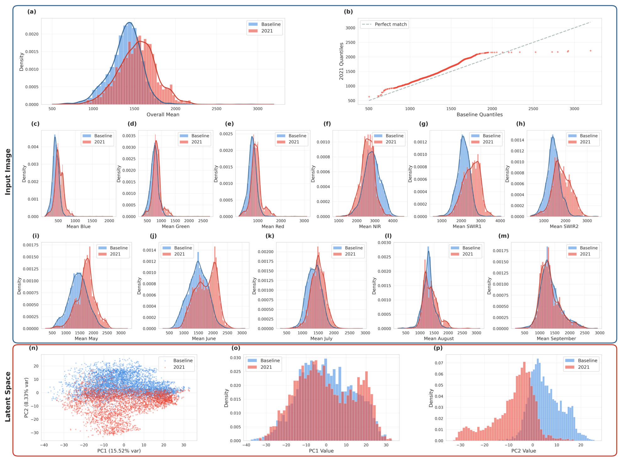
Detecting the 2021 Drift. Figure 1 presents a comparison between the baseline distribution and the 2021 growing season at the PA patch level. In the input space, the overall mean distribution for 2021 is right-shifted relative to the baseline with the Q-Q plot exhibiting systematic deviations and heavier upper tails. This indicates a pronounced covariate shift. Band-wise analyses reveal coherent mean shifts across all spectral channels (particularly NIR and SWIR), though substantial overlap remains. In the latent space, the distributional shift becomes more structured. Using the baseline-fit PCA defined in Section 2.3.1, the projections show that the separation between baseline and 2021 samples is driven primarily by the second principal component (PC2), while PC1 distributions largely overlap. The PC2 distribution for 2021 exhibits a clear shift in both location and shape. This indicates that the foundation model encodes the 2021 drift as a directional change within a specific latent subspace rather than as a uniform shift.

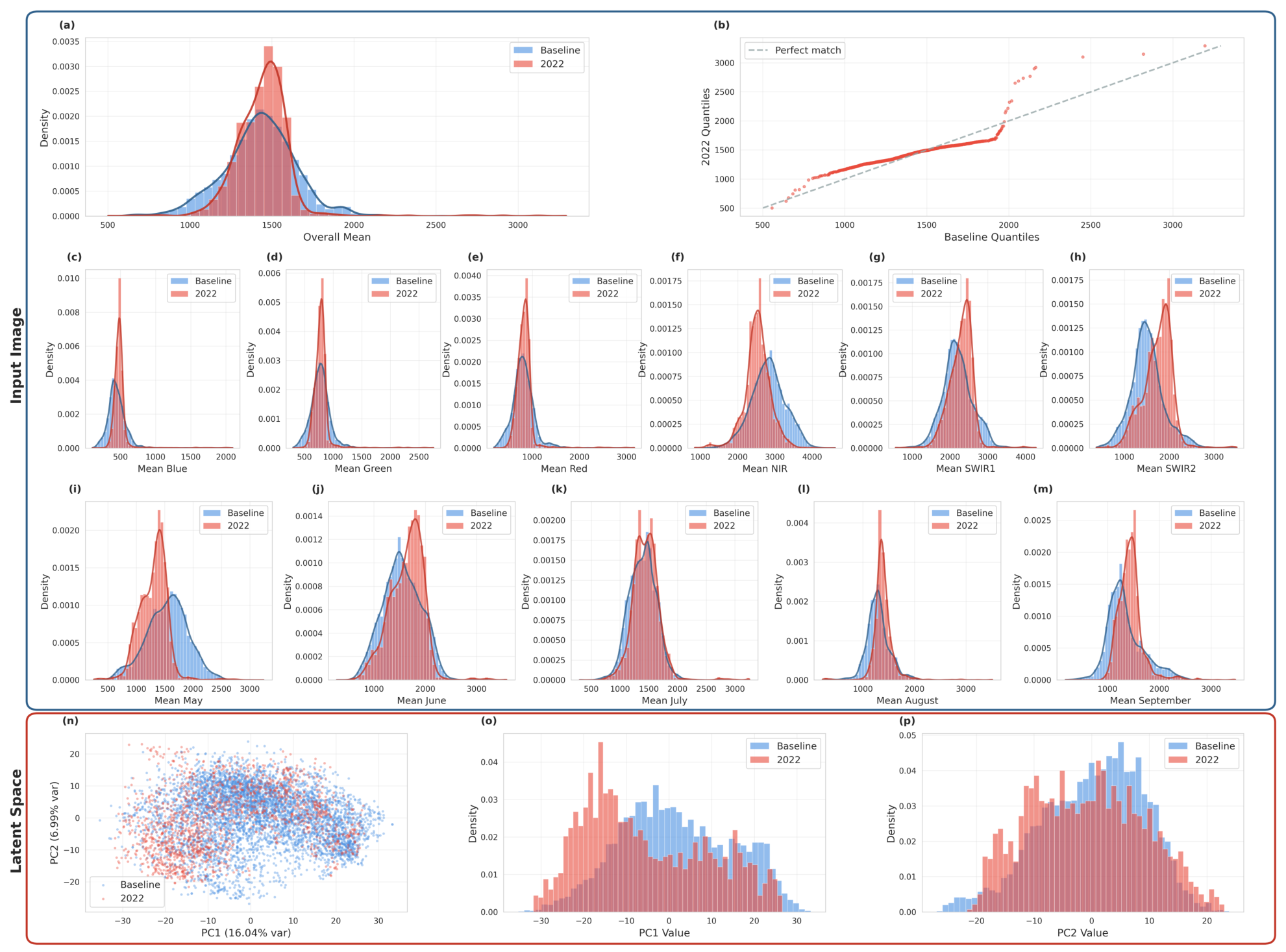
Verifying Stability in 2022. In contrast to the pronounced shifts observed for 2021, the 2022 growing season closely aligns with the baseline distribution in both input and latent spaces (Figure 2). The normalized distance distributions for 2022 largely overlap with those of the reference years. This is reflected in the substantially smaller dispersion of latent-space distances and a lower correlation between input- and latent-space drift metrics ($r\approx 0.46$) compared to the stronger coupling observed for 2021 ($r\approx 0.75$). These results confirm that our framework correctly identifies 2022 as an in-distribution reference year and 2021 as an OOD year.

These observations lead to three properties of the Catch mechanism. First, latent-space Mahalanobis distance is more sensitive to true distribution drift than input-space metrics. Second, normalization and baseline construction are essential for cross-space and cross-year comparisons. Third, comparing a single year against the aggregate training-year baseline provides a label-free signal for detecting OOD years. We define the Catch trigger as a statistically significant shift in the normalized latent Mahalanobis distribution for a given year relative to its baseline, which is supported by increased alignment between input and latent distances. Nevertheless, the detection of distributional drift alone does not necessarily imply that a sample will incur a high prediction error. In our next experiment, we explore the relationship between drift metrics and prediction error across both county and patch scales.

3.2. The Disconnect: Drift vs. Prediction Error

Having established that our metrics can detect drift, we next evaluate whether distributional distance metrics can serve as reliable indicators of prediction error. A common assumption in drift-aware monitoring is that model reliability degrades as inputs deviate from the training manifold [27,28]; here, we explicitly examine whether samples exhibiting larger statistical distances from the baseline distribution also incur higher yield estimation error. To this end, chip- and patch-level RMSE values are compared against Mahalanobis, Euclidean, and cosine distance metrics computed in both the input spectral space and the learned latent representation space. These analyses are conducted across spatial scales and for both county-level and PA-level datasets. The results of the FARM-C and FARM-PA model performance are show in

Table 1. FARM-C and FARM-PA model performance.

Model	RMSE	MAE	R2
FARM-C	0.4418	0.3482	0.7803
FARM-PA	0.6584	0.492	0.7271

.

Table 2. Aggregate evaluation accuracy of the FARM models on the in-distribution control year (2022) and the out-of-distribution drift year (2021).

Model	Year	RMSE	MAE
FARM-C	2022 (control)	0.425	0.348
	2021 (drift)	0.581	0.414
FARM-PA	2022 (control)	0.653	0.483
	2021 (drift)	0.792	0.579

expresses model stability directly in terms of accuracy: moving from the control year (2022) to the drift year (2021), the aggregate RMSE of FARM-C changes from 0.425 to 0.581 and that of FARM-PA from 0.653 to 0.792. The comparatively modest degradation in aggregate accuracy, despite the pronounced latent-space drift documented in Section 3.1, is the accuracy-level counterpart of the per-sample disconnect analyzed below: a large distributional shift does not translate into a proportionate loss of predictive accuracy.

3.2.1. County Level

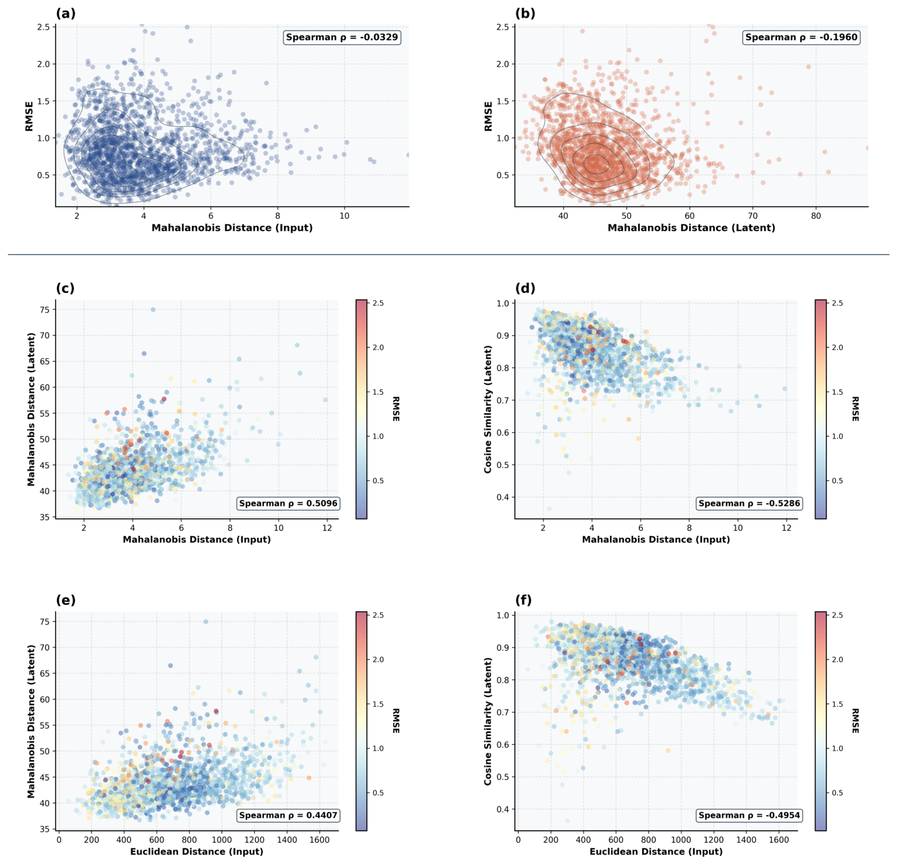
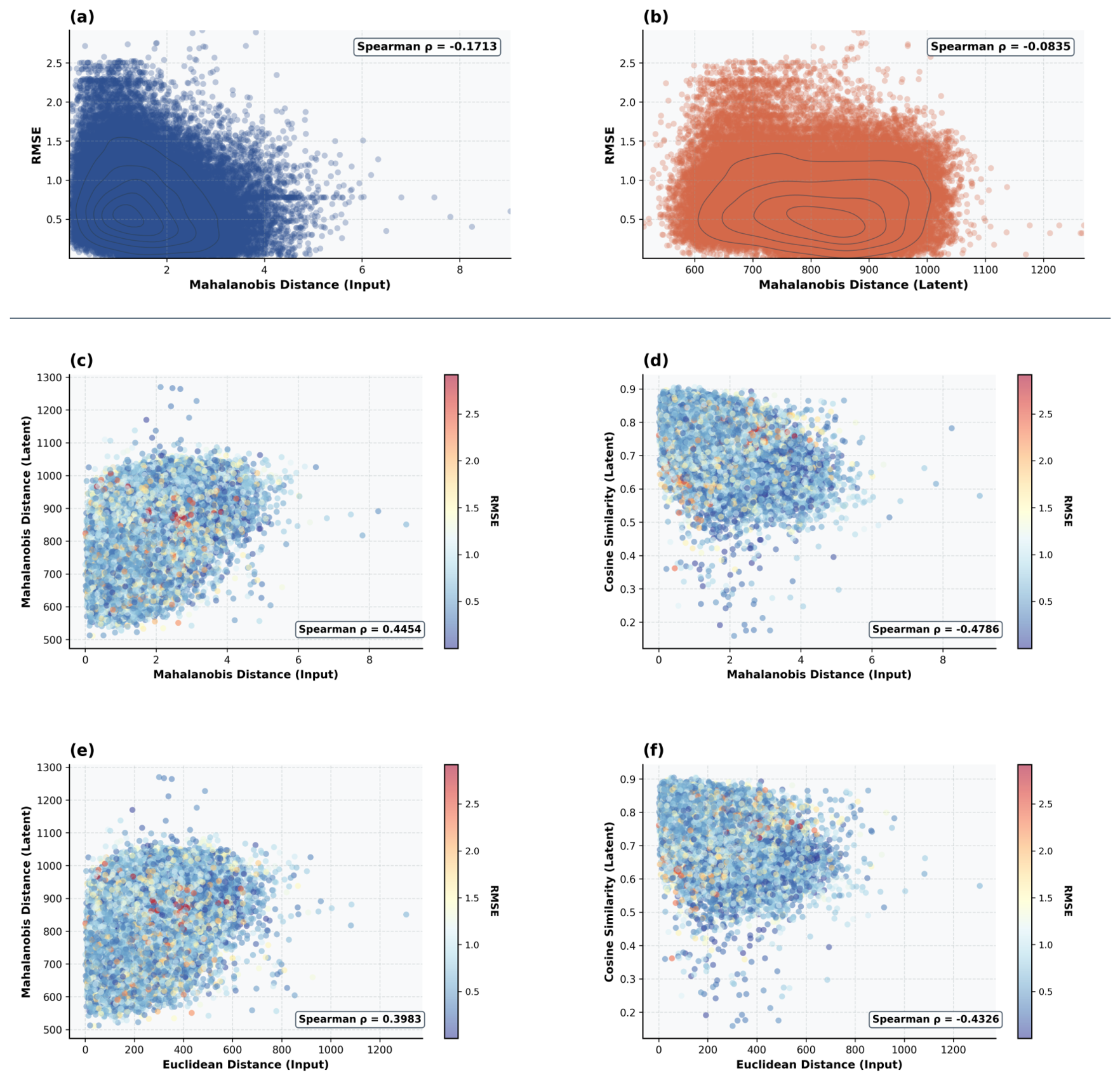
Figure 3 summarizes the results for the 2021 growing season—identified as a drift year—using the FARM-C model and county-level ground-truth yields at the chip level. Contrary to the expectation that larger distributional distance corresponds to increased error, we observe no strong positive relationship between drift magnitude and RMSE. Scatter plots of RMSE versus Mahalanobis distance in both the input space and latent space (Figure 3a,b) show that some counties with the largest drift scores incur low prediction error, while several samples that are close to the training distribution exhibit large RMSE values.

Spearman rank correlations [29] between distance metrics and RMSE are weak or negative ($\rho =-0.03$ for input-space and $\rho =-0.20$ for latent-space Mahalanobis distance), indicating that distance alone explains little of the observed error variability. While latent-space Mahalanobis distance exhibits greater sensitivity to distributional shift than its input-space counterpart, this increased sensitivity does not translate into reliable error prediction. Similar behavior is observed for cosine similarity and input-space Euclidean distance (Figure 3c–f).

3.2.2. PA Level

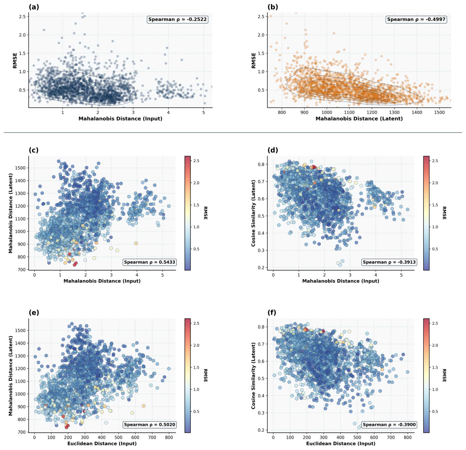
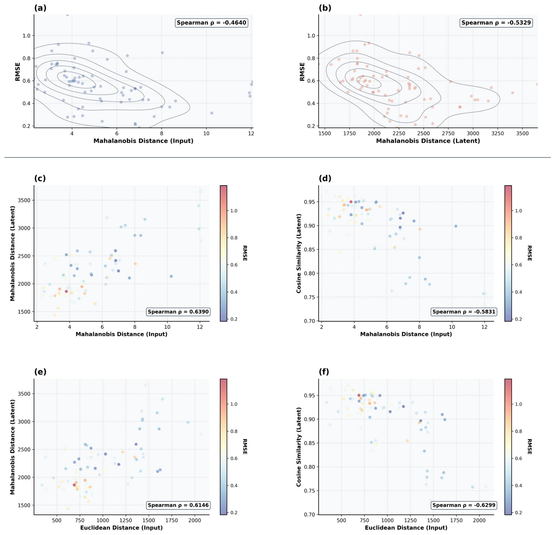
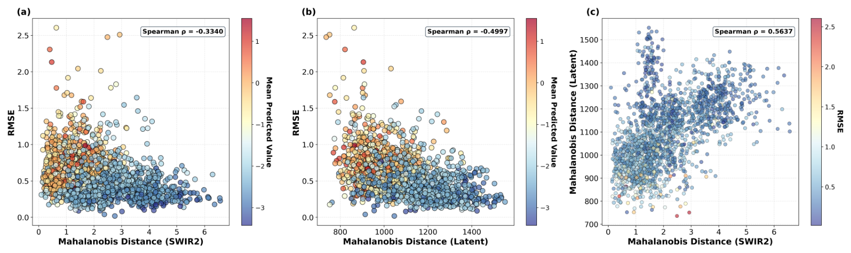
At the PA scale, we observe stronger monotonic relationships between drift metrics and prediction error compared to the county-level analysis, particularly in the latent space. Figure 4a,b plot patch-level RMSE against Mahalanobis distance in both the input and latent spaces for the 2021 growing season. While the input-space Mahalanobis distance exhibits a moderate negative Spearman correlation with RMSE ($\rho \approx -0.36$), the latent-space Mahalanobis distance shows a substantially stronger negative association ($\rho \approx -0.50$). This indicates that patches that are more distant in latent space are, on average, predicted with lower error [30].

Despite this stronger correlation, the scatter remains broad with considerable overlap across the drift spectrum: patches with large latent distances can still incur low or moderate error and vice versa. Similar behavior is observed when comparing input-space distances to latent-space cosine similarity (Figure 4c–f), where moderate correlations reflect structured drift without yielding a sharp separation between low- and high-error samples. Overall, although latent-space metrics are more sensitive to distributional shift at the PA level, distributional distance alone remains insufficient as a reliable proxy for prediction error. This suggests that the model can remain accurate on some distributionally distant samples.

To further validate the consistency of these findings across spatial resolutions, we extend this analysis to alternate cross-scale configurations in Appendix A, where county-level data are examined at the patch scale and PA-level data are examined at the chip scale.

3.3. Fine-Grained Analysis

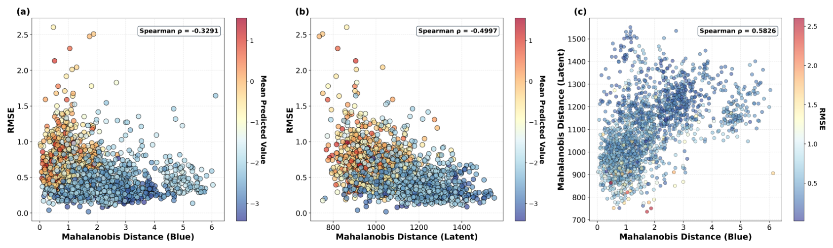
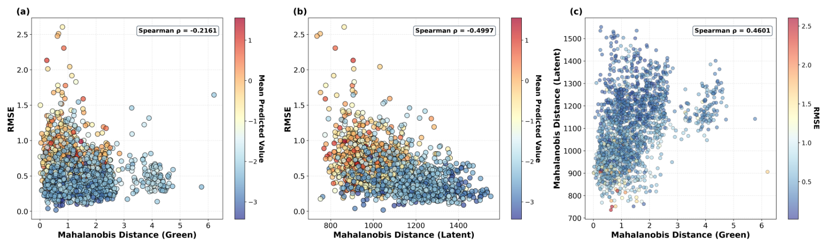
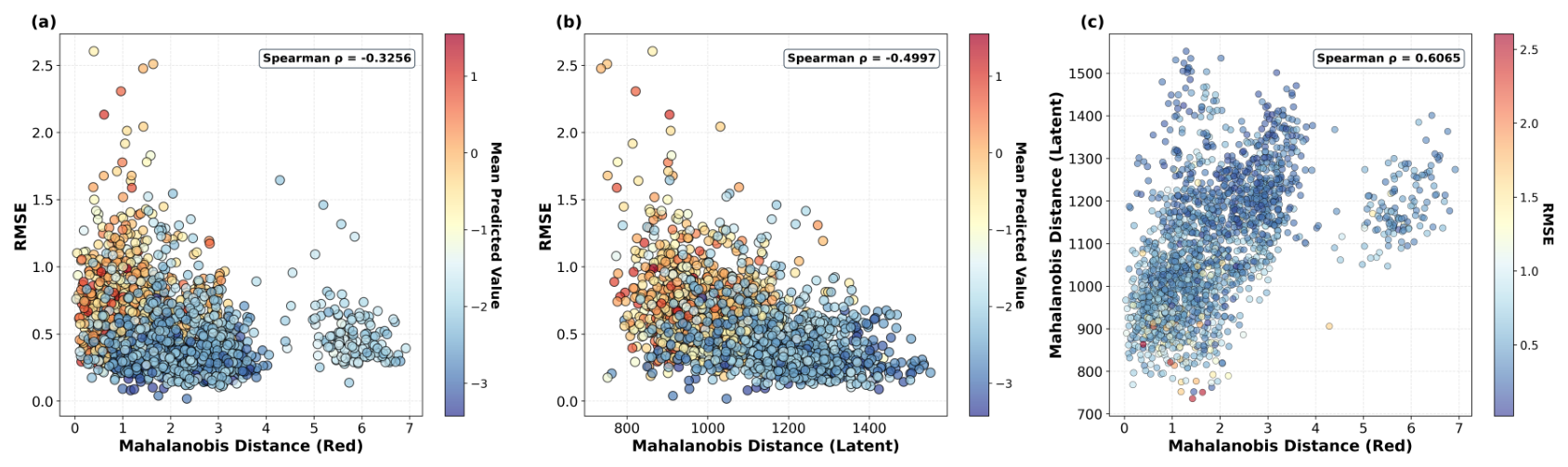
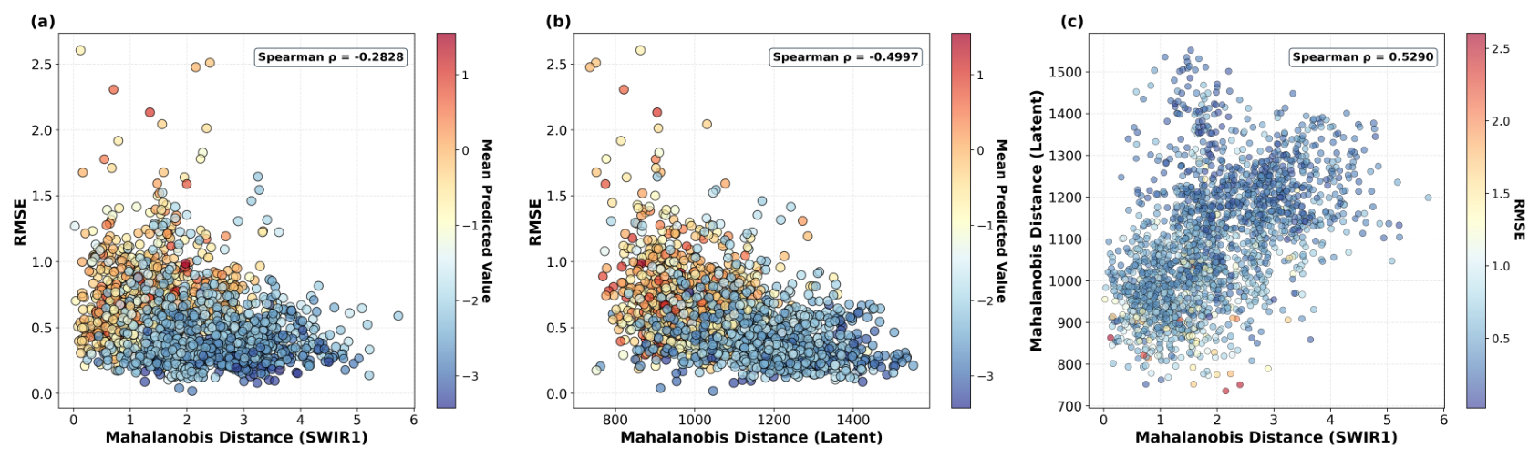
This experiment was motivated by our prior exploratory interpretability analysis of the FARM model, which showed that certain months and spectral bands contribute more strongly to yield prediction [13]. We therefore examined whether the degree of drift in each individual spectral band or monthly composite would exhibit a different relationship with RMSE when analyzed in isolation. To this end, we computed Mahalanobis, Euclidean, and cosine distances separately for each of the six spectral bands and for each monthly composite from May through September, and we correlated these per-band and per-month drift measures with prediction error.

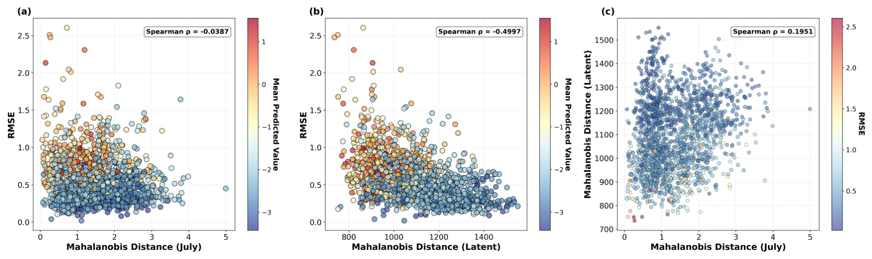
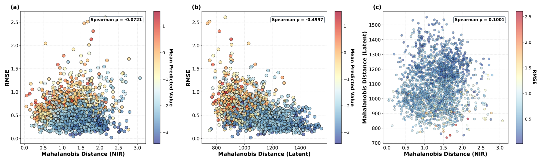
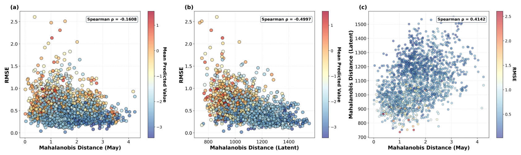
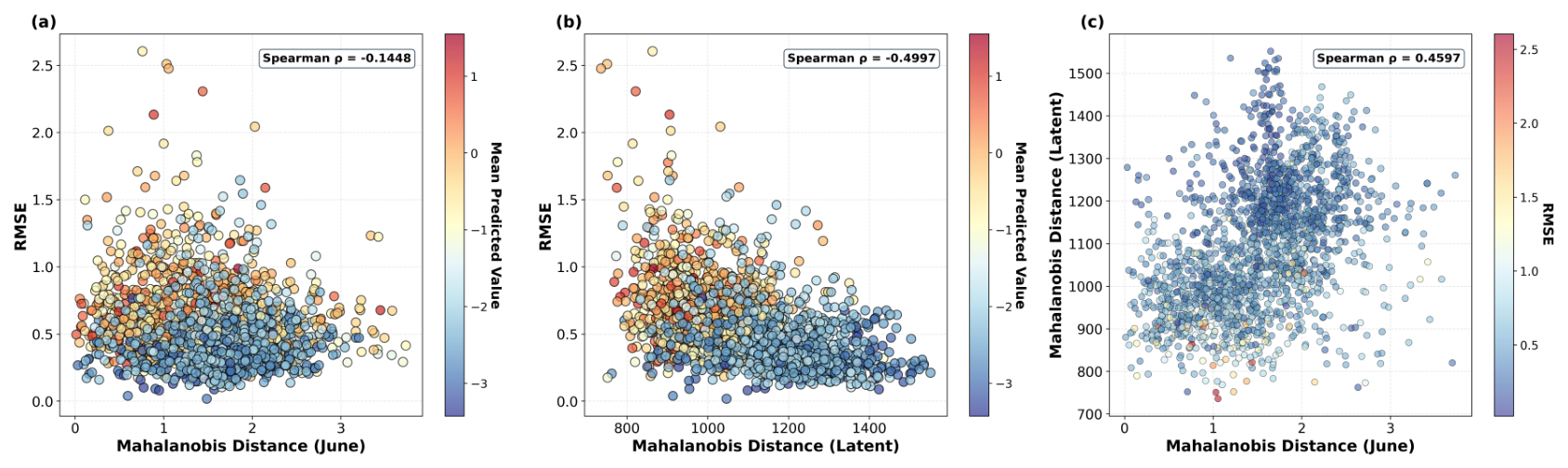
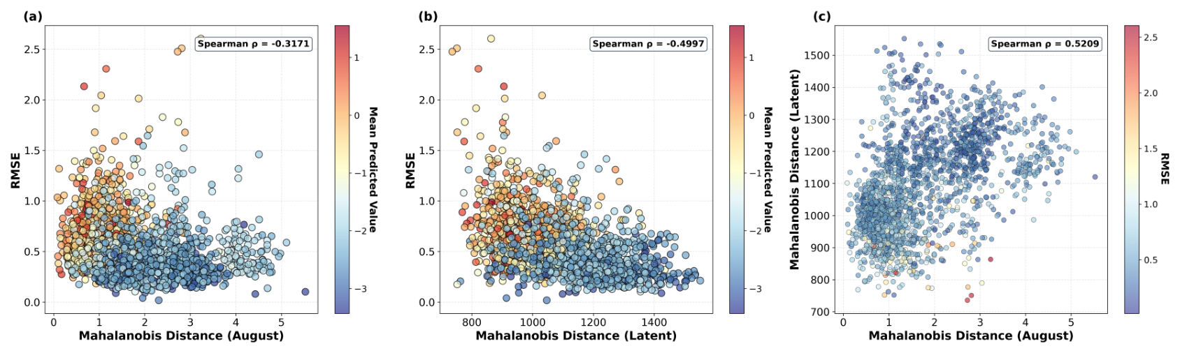
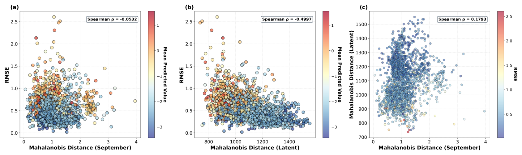
Although space constraints prevent us from presenting all results, Figure 5 and Figure 6 illustrate representative cases. The complete set of figures for all spectral bands and monthly composites is provided in Appendix B. In particular, Figure 5 shows RMSE plotted against Mahalanobis distance in both the input (image) space and the latent space for the July composite, while Figure 6 presents the same analysis for the NIR band. In both cases, Mahalanobis distance in the latent space exhibits a substantially stronger negative Spearman correlation with RMSE than the corresponding image-space Mahalanobis distance, while input-space drift shows only a weak or negligible association with error magnitude despite statistical significance driven by sample size. Color-coding points by normalized true yield in Figure 5a,b reveals no clear relationship between yield magnitude and RMSE: both low- and high-yield samples achieve low prediction error across the latent drift spectrum. This indicates that the observed latent-space correlation with RMSE is not driven by extreme yield values but instead reflects properties of the learned representation.

Importantly, despite the stronger latent-space correlation, the overall trend remains inconsistent and non-predictive: large drift values—whether computed per band or per month—do not reliably correspond to high RMSE values. This observation holds across all spectral bands and temporal composites. These results reinforce our earlier findings that distributional drift, even when isolated to specific bands or phenological stages, is not a reliable proxy for performance degradation. The FARM model is therefore able to extrapolate into drifted spectral–temporal regimes without systematically incurring large prediction errors; we report this extrapolation as the explanation for the band- and month-level drift-error decoupling rather than as a guarantee of robustness.

4. Discussion

The results support two principal findings. First, distance metrics computed in the model’s latent space, particularly latent-space Mahalanobis distance, detect the 2021 growing season as anomalous more clearly than the corresponding input-space metrics. The shift is expressed as a directional change confined to a specific latent subspace (PC2) rather than as a uniform displacement. Second, and more consequentially for operational use, the magnitude of this distributional shift is a poor predictor of prediction error: across county and PA scales and across individual spectral bands and monthly composites, large drift scores do not reliably coincide with high RMSE, and some of the most out-of-distribution samples are among the most accurately predicted.

The higher sensitivity of latent-space metrics is consistent with evidence from medical-imaging and radiological monitoring, where distances computed in learned representations provide an earlier and cleaner warning of data shift than input-space statistics [17,21]. Our results extend this observation to agricultural geospatial foundation models for which such metrics had not previously been evaluated systematically. A plausible mechanism is that the Prithvi backbone encodes seasonal phenology, so a drought year manifests as a structured directional shift in the latent manifold even where raw spectral distributions still overlap substantially with the baseline [11].

The disconnect between drift magnitude and prediction error is this paper’s most important result, and it runs counter to a common assumption in drift-aware monitoring: that model reliability degrades monotonically as inputs move away from the training manifold [27,28]. Our findings instead align with work showing that distance- and uncertainty-based signals can decouple from actual error under dataset shift [30]. They also align with the broader observation that aggregate in-distribution behavior does not translate into reliable per-sample error prediction once the distribution moves [22]. The negative rank correlation at the PA scale (latent-space Spearman $\rho \approx -0.50$ versus input-space $\rho \approx -0.36$), in which more distant patches are on average predicted with lower error, is counter-intuitive under the manifold-distance assumption but is consistent with the strong extrapolation capacity reported for the FARM models on distributionally distant inputs [13].

The relationship between drift and error is also data resolution dependent. At the county scale, the association is weak or negligible, whereas at the PA scale, it strengthens but remains broad with substantial overlap between low- and high-error samples across the drift spectrum. We attribute part of this contrast to spatial aggregation and to the coarse, potentially noisy county-level labels in which a single yield value is assigned to an entire administrative unit. The high-error in-distribution cases are therefore better explained by label and measurement uncertainty—the label-drift mechanism introduced in Section 2—than by distributional novelty, reinforcing the conclusion that distance alone cannot serve as a proxy for predictive reliability.

Limitations and Operational Implications

Taken together, these results carry an operational implication: the reliable deployment of agricultural foundation models requires monitoring that distinguishes distributional novelty from genuinely harmful performance degradation, pairing drift detection with explicit error- or uncertainty-aware estimation rather than relying on distance thresholds alone. For the FARM framework specifically, this suggests a two-stage operational design. Latent-space Mahalanobis distance is inexpensive, label-free, and computable at the inference time, and it can therefore serve as an early-warning flag for anomalous growing seasons such as 2021. However, because a large drift score does not imply a large prediction error in our experiments, such a flag must not be used on its own to gate, down-weight, or abstain on predictions: doing so would discard the accurate predictions that FARM produces on many out-of-distribution inputs while failing to catch the high-error in-distribution samples that distance does not flag. We therefore recommend that an operational FARM pipeline couple the Catch (drift-detection) stage with an explicit per-sample error- or uncertainty-estimation stage before any Adapt action is taken, and that, in the interim, regions flagged as drifted be routed to human or agronomic review and targeted ground-truth collection rather than being automatically rejected.

Several limitations bound the scope of these conclusions. First, our evaluation focuses on a single, agronomically verified drift event, the 2021 Canadian Prairie drought, as it is the only such anomaly documented within our 2018–2023 record. The drift–error disconnect is therefore established for one drift mechanism; confirming that it generalizes to other anomaly types, such as flooding, heat stress, or pest outbreaks, will require multi-event datasets and is an important direction for future work. Second, the findings are conditional on two fixed baselines (FARM-C and FARM-PA) both built on the Prithvi-EO-2.0-600M backbone; whether the same decoupling holds for other architectures or task heads is untested. Third, the input-space drift descriptor pools reflectance into a two-dimensional (mean, standard deviation) summary and so cannot, in isolation, resolve drift confined to an individual band or phenological stage. Fourth, the coarse, up-sampled county-level labels act as a confound in the county-scale analysis and are a plausible source of the high-error in-distribution cases. Finally, this paper is diagnostic: we do not calibrate the drift detector to a fixed operational decision threshold nor do we implement the complementary error- or uncertainty-estimation stage (the deferred Adapt phase) that our results motivate. Addressing these limitations, particularly the integration and validation of an explicit error-estimation stage across multiple independent drift events, is the principal focus of future work.

5. Conclusions

This paper presents a systematic reliability analysis framework for the FARM model under distribution drift. Using Mahalanobis, cosine, and Euclidean distances in both input and latent spaces, we showed that representation-aware metrics can effectively detect distributional drift, including the anomalous 2021 growing season, while also demonstrating that large drift scores do not necessarily correspond to large prediction errors. As discussed in Section 4, this disconnect between drift detection and predictive unreliability means that distributional distance alone is insufficient for operational reliability assessment and that robust deployment requires monitoring able to separate distributional novelty from harmful performance degradation. Future work will extend this framework along several directions. These include error-aware drift indicators, a tighter integration of uncertainty estimation with representation-space metrics [31,32,33], and adaptation strategies that distinguish harmful shifts from benign distributional change [34]. We also plan evaluation across additional independent drift events and analysis of the causal drivers underlying the mismatch between drift magnitude and prediction error.

References

1. Li, H.; Porth, L.; Tan, K.S.; Zhu, W. Improved index insurance design and yield estimation using a dynamic factor forecasting approach. Insur. Math. Econ. 2021, 96, 208–221. [Google Scholar] [CrossRef]
2. Basso, B.; Liu, L. Chapter Four—Seasonal crop yield forecast: Methods, applications, and accuracies. In Advances in Agronomy; Academic Press: Cambridge, MA, USA, 2019; Volume 154, pp. 201–255. [Google Scholar] [CrossRef]
3. Lobell, D.B.; Schlenker, W.; Costa-Roberts, J. Climate Trends and Global Crop Production Since 1980. Science 2011, 333, 616–620. [Google Scholar] [CrossRef] [PubMed]
4. Lesk, C.; Rowhani, P.; Ramankutty, N. Influence of extreme weather disasters on global crop production. Nature 2016, 529, 84–87. [Google Scholar] [CrossRef] [PubMed]
5. Wheaton, E.; Kulshreshtha, S. Adaptations to prairie drought by farmers and ranchers. Prairie Forum 2008, 33, 99–123. [Google Scholar]
6. Khaki, S.; Wang, L.; Archontoulis, S.V. A CNN-RNN framework for crop yield prediction. Front. Plant Sci. 2020, 10, 1750. [Google Scholar] [CrossRef] [PubMed]
7. Leng, G.; Hall, J. Crop yield sensitivity of global major agricultural countries to droughts and the projected changes in the future. Sci. Total Environ. 2019, 654, 811–821. [Google Scholar] [CrossRef] [PubMed]
8. Tian, H.; Wang, P.; Tansey, K.; Zhang, J.; Zhang, S.; Li, H. An LSTM neural network for improving wheat yield estimates by integrating remote sensing data and meteorological data in the Guanzhong Plain, PR China. Agric. For. Meteorol. 2021, 310, 108629. [Google Scholar] [CrossRef]
9. Tuia, D.; Persello, C.; Bruzzone, L. Domain adaptation for the classification of remote sensing data: An overview of recent advances. IEEE Geosci. Remote Sens. Mag. 2016, 4, 41–57. [Google Scholar] [CrossRef]
10. Wulder, M.A.; Roy, D.P.; Radeloff, V.C.; Loveland, T.R.; Anderson, M.C.; Johnson, D.M.; Healey, S.; Zhu, Z.; Scambos, T.A.; Pahlevan, N.; et al. Fifty years of Landsat science and impacts. Remote Sens. Environ. 2022, 280, 113195. [Google Scholar] [CrossRef]
11. Szwarcman, D.; Roy, S.; Fraccaro, P.; Gíslason, Þ.E.; Blumenstiel, B.; Ghosal, R.; de Oliveira, P.H.; Almeida, J.L.D.S.; Sedona, R.; Kang, Y.; et al. Prithvi-eo-2.0: A versatile multi-temporal foundation model for earth observation applications. arXiv 2024, arXiv:2412.02732. [Google Scholar]
12. Jakubik, J.; Yang, F.; Blumenstiel, B.; Scheurer, E.; Sedona, R.; Maurogiovanni, S.; Bosmans, J.; Dionelis, N.; Marsocci, V.; Kopp, N.; et al. TerraMind: Large-Scale Generative Multimodality for Earth Observation. In Proceedings of the IEEE/CVF International Conference on Computer Vision (ICCV), Honolulu, HI, USA, 19–23 October 2025; pp. 7383–7394. [Google Scholar]
13. Nejadshamsi, S.; Zhang, Y.; Porth, B.; Zaki, S.; Porth, L.; Khoshdel, V. FARM: Crop Yield Prediction via Regression on Prithvi’s Encoder for Satellite Sensing. AgriEngineering 2026, 8, 2. [Google Scholar] [CrossRef]
14. He, K.; Chen, X.; Xie, S.; Li, Y.; Dollár, P.; Girshick, R. Masked Autoencoders Are Scalable Vision Learners. In Proceedings of the IEEE/CVF Conference on Computer Vision and Pattern Recognition (CVPR), New Orleans, LA, USA, 21–24 June 2022; pp. 16000–16009. [Google Scholar] [CrossRef]
15. Lu, J.; Liu, A.; Dong, F.; Gu, F.; Gama, J.; Zhang, G. Learning under concept drift: A review. IEEE Trans. Knowl. Data Eng. 2018, 31, 2346–2363. [Google Scholar] [CrossRef]
16. Gama, J.; Žliobaitė, I.; Bifet, A.; Pechenizkiy, M.; Bouchachia, A. A survey on concept drift adaptation. ACM Comput. Surv. 2014, 46, 44. [Google Scholar] [CrossRef] [PubMed]
17. Zamzmi, G.; Venkatesh, K.; Nelson, B.; Prathapan, S.; Yi, P.; Sahiner, B.; Delfino, J.G. Out-of-distribution detection and radiological data monitoring using statistical process control. J. Imaging Inform. Med. 2024, 38, 997–1015. [Google Scholar] [CrossRef] [PubMed]
18. Mahalanobis, P.C. On the generalized distance in statistics. Proc. Natl. Inst. Sci. India 1936, 2, 49–55. [Google Scholar]
19. Singhal, A. Modern information retrieval: A brief overview. IEEE Data Eng. Bull. 2001, 24, 35–43. [Google Scholar]
20. Deza, E.; Deza, M.M. Encyclopedia of Distances; Springer: Berlin/Heidelberg, Germany, 2009. [Google Scholar] [CrossRef]
21. Yang, J.; Zhou, K.; Li, Y.; Liu, Z. Generalized Out-of-Distribution Detection: A Survey. arXiv 2021, arXiv:2110.11334. [Google Scholar]
22. Miller, J.P.; Taori, R.; Raghunathan, A.; Sagawa, S.; Koh, P.W.; Sagawa, S.; Liang, P.; Carmon, Y.; Schmidt, L. Accuracy on the Line: On the Strong Correlation Between Out-of-Distribution and In-Distribution Generalization. In Proceedings of the International Conference on Machine Learning (ICML), PMLR, Virtual, 18–24 July 2021; pp. 7721–7735. [Google Scholar]
23. ICLR 2026 CAO Workshop Organizers. Catch, Adapt, and Operate (CAO): Monitoring ML Models Under Drift. In Proceedings of the ICLR 2026 Workshop, Rio de Janeiro, Brazil, 23–27 April 2026.
24. Lee, K.; Lee, K.; Lee, H.; Shin, J. A Simple Unified Framework for Detecting Out-of-Distribution Samples and Adversarial Attacks. In Proceedings of the Advances in Neural Information Processing Systems (NeurIPS), Montreal, QC, Canada, 3–8 December 2018; Volume 31. [Google Scholar]
25. Nalisnick, E.; Matsukawa, A.; Teh, Y.W.; Gorur, D.; Lakshminarayanan, B. Do deep generative models know what they don’t know? In Proceedings of the International Conference on Learning Representations (ICLR), New Orleans, LA, USA, 6–9 May 2019. [Google Scholar]
26. Agriculture and Agri-Food Canada. Drought Conditions in the Canadian Prairies: 2021 Season Overview; Technical report; Agriculture and Agri-Food Canada: Ottawa, ON, Canada, 2021.
27. Hendrycks, D.; Gimpel, K. A Baseline for Detecting Misclassified and Out-of-Distribution Examples in Neural Networks. In Proceedings of the International Conference on Learning Representations (ICLR), Toulon, France, 24–26 April 2017. [Google Scholar]
28. Lakshminarayanan, B.; Pritzel, A.; Blundell, C. Simple and Scalable Predictive Uncertainty Estimation using Deep Ensembles. In Proceedings of the Advances in Neural Information Processing Systems (NeurIPS), Long Beach, CA, USA, 4–9 December 2017; Volume 30. [Google Scholar]
29. Spearman, C. The proof and measurement of association between two things. Am. J. Psychol. 1904, 15, 72–101. [Google Scholar] [CrossRef] [PubMed]
30. Ovadia, Y.; Fertig, E.; Ren, J.; Nado, Z.; Sculley, D.; Nowozin, S.; Dillon, J.V.; Lakshminarayanan, B.; Snoek, J. Can You Trust Your Model’s Uncertainty? Evaluating Predictive Uncertainty Under Dataset Shift. In Proceedings of the Advances in Neural Information Processing Systems (NeurIPS), Vancouver, BC, Canada, 8–14 December 2019; Volume 32. [Google Scholar]
31. Angelopoulos, A.N.; Bates, S. Conformal Prediction: A Gentle Introduction. Found. Trends Mach. Learn. 2023, 16, 494–591. [Google Scholar] [CrossRef]
32. Gal, Y.; Ghahramani, Z. Dropout as a Bayesian Approximation: Representing Model Uncertainty in Deep Learning. In Proceedings of the International Conference on Machine Learning (ICML), PMLR, New York, NY, USA, 20–22 June 2016; pp. 1050–1059. [Google Scholar]
33. De Lange, M.; Aljundi, R.; Masana, M.; Parisot, S.; Jia, X.; Leonardis, A.; Slabaugh, G.; Tuytelaars, T. A Continual Learning Survey: Defying Forgetting in Classification Tasks. IEEE Trans. Pattern Anal. Mach. Intell. 2021, 44, 3366–3385. [Google Scholar] [CrossRef] [PubMed]
34. Geifman, Y.; El-Yaniv, R. Selective prediction in deep neural networks. In Proceedings of the Advances in Neural Information Processing Systems (NeurIPS), Long Beach, CA, USA, 4–9 December 2017; Volume 30. [Google Scholar]
Figure 1. Comprehensive distribution comparison between the baseline years and the 2021 growing season at the PA patch level. Panels (a,b) report the overall input-space mean: (a) histogram with kernel-density estimate (KDE) of the patch-level overall mean for the baseline and 2021; (b) the corresponding quantile–quantile (Q–Q) plot with the dashed line indicating perfect agreement. Panels (ch) show the band-wise input-space mean distributions for (c) blue, (d) green, (e) red, (f) NIR, (g) SWIR1 and (h) SWIR2. Panels (im) show the month-wise input-space mean distributions for (i) May, (j) June, (k) July, (l) August and (m) September. Panels (np) summarize the latent space: (n) scatter of the first two principal components (PC1 vs. PC2) of the latent embeddings; (o) the PC1 marginal distribution; (p) the PC2 marginal distribution. In all panels, blue denotes the baseline and red the 2021 test year; rows 1–3 correspond to the input image space and row 4 to the latent space.
Remotesensing 18 02416 g001
Figure 2. Comprehensive distribution comparison between the baseline years and the 2022 growing season at the PA patch level. Panels (a,b) report the overall input-space mean: (a) histogram with kernel-density estimate (KDE) of the patch-level overall mean for the baseline and 2022; (b) the corresponding quantile–quantile (Q–Q) plot with the dashed line indicating perfect agreement. Panels (ch) show the band-wise input-space mean distributions for (c) blue, (d) green, (e) red, (f) NIR, (g) SWIR1 and (h) SWIR2. Panels (im) show the month-wise input-space mean distributions for (i) May, (j) June, (k) July, (l) August and (m) September. Panels (np) summarize the latent space: (n) scatter of the first two principal components (PC1 vs. PC2) of the latent embeddings; (o) the PC1 marginal distribution; (p) the PC2 marginal distribution. In all panels, blue denotes the baseline and red the 2022 test year; rows 1–3 correspond to the input image space and row 4 to the latent space.
Remotesensing 18 02416 g002
Figure 3. Reliability analysis of the FARM-C model under 2021 distribution drift at the county chip level. Panels (a,b) show the error–distance relationship: chip-level RMSE against Mahalanobis distance in (a) the input spectral space and (b) the latent embedding space. Panels (cf) show the multi-space metric comparison between input-space and latent-space distance metrics: (c) input Mahalanobis vs. latent Mahalanobis distance, (d) input Mahalanobis distance vs. latent cosine similarity, (e) input Euclidean vs. latent Mahalanobis distance, and (f) input Euclidean distance vs. latent cosine similarity. In panels (cf), points are color-coded by RMSE to visualize the distribution of error across the drift spectrum. The Spearman rank correlation ρ is annotated within each panel. RMSE is expressed in normalized yield units.
Remotesensing 18 02416 g003
Figure 4. Reliability analysis of the FARM-PA model under 2021 distribution drift at the PA patch level. Panels (a,b) show the error–distance relationship: patch-level RMSE against Mahalanobis distance in (a) the input spectral space and (b) the latent embedding space. Panels (cf) show the multi-space metric comparison between input-space and latent-space distance metrics: (c) input Mahalanobis vs. latent Mahalanobis distance, (d) input Mahalanobis distance vs. latent cosine similarity, (e) input Euclidean vs. latent Mahalanobis distance, and (f) input Euclidean distance vs. latent cosine similarity. In panels (cf), points are color-coded by RMSE to visualize the distribution of error across the drift spectrum. The Spearman rank correlation ρ is annotated within each panel.
Remotesensing 18 02416 g004
Figure 5. PA-level patch-wise analysis for the 2021 drift year (July composite). (a) RMSE vs. input-space Mahalanobis distance. (b) RMSE vs. latent-space Mahalanobis distance. (c) Input-space vs. latent-space Mahalanobis distance. Points in (a,b) are color-coded by normalized true yield; points in (c) are color-coded by RMSE.
Remotesensing 18 02416 g005
Figure 6. PA-level patch-wise analysis for the 2021 drift year (NIR). (a) RMSE vs. input-space Mahalanobis distance. (b) RMSE vs. latent-space Mahalanobis distance. (c) Input-space vs. latent-space Mahalanobis distance. Points in (a,b) are color-coded by normalized true yield; points in (c) are color-coded by RMSE.
Remotesensing 18 02416 g006