On the Use of SAR Images for Predicting Vegetation Indices: Challenges and Limitations

Highlights

What are the main findings?

• An investigation of how an SAR-to-multispectral reconstruction framework can produce vegetation indices statistically equivalent to dedicated SAR-to-index-specific models.
• An ablation study on the use of SAR and WorldCover inputs and on the use of the conventional evaluation metrics that yields statistically indistinguishable reconstruction performance across all evaluated indices.

What are the implications of the main findings?

• A single multispectral reconstruction model can replace multiple dedicated indexspecific models, reducing training overhead while preserving accuracy.
• The use of solely conventional metrics (MAE, PSNR, SSIM) does not represent the real quantitative performance of the reconstruction models, thus more discriminative evaluation protocols are needed.

Abstract

Optical vegetation and soil indices are widely used in Earth observation, although their estimation is strongly affected by cloud coverage and illumination variability. Synthetic-aperture radar (SAR) has therefore attracted increasing interest as an alternative source for spectral index prediction. Most existing studies focus on directly estimating a single index from SAR observations. In this work, we investigate a more flexible formulation in which Sentinel-2 multispectral bands are first reconstructed from Sentinel-1 SAR data and subsequently used to derive multiple spectral indices. Experiments are conducted on the SEN12TP dataset, exploiting near-synchronous paired Sentinel-1 and Sentinel-2 acquisitions together with auxiliary elevation and land-cover information. Three SAR-to-multispectral reconstruction strategies are compared, namely, Efficient-UNet, Pix2Pix, and a conditional flow matching model. The resulting indices are then evaluated against those obtained through dedicated index-specific reconstruction models. The results show that Efficient-UNet achieves the best overall multispectral reconstruction performance among the evaluated architectures. Moreover, indices derived from reconstructed multispectral bands achieve performance comparable to dedicated index-specific models while offering substantially greater flexibility, as multiple indices can be computed within a single framework without retraining task-specific models. At the same time, the experiments highlight important intrinsic limitations of SAR-based spectral reconstruction. Although the reconstructed products preserve the large-scale spatial organization of the scenes, they do not fully recover fine spectral and vegetation-sensitive details. Consequently, SAR-derived spectral indices should be regarded as approximate proxies of optical observations rather than direct substitutes, particularly in applications requiring accurate biophysical interpretation.

1. Introduction

Monitoring the Earth’s surface is essential for understanding how land conditions evolve over time and how such variations affect vegetation status, water bodies, and other environmental dynamics. These aspects are particularly relevant in applications such as precision agriculture and environmental monitoring [1]. To describe these dynamics, several spectral indices are commonly used, including the Normalized Difference Vegetation Index (NDVI), the Normalized Difference Water Index (NDWI), and the Soil-Adjusted Vegetation Index (SAVI), among others [2]. These indices are typically derived from multispectral optical imagery.

In this context, synthetic-aperture radar (SAR) has attracted increasing interest because, unlike optical data, it is not affected by cloud cover and does not depend on solar illumination [3,4]. Recent studies have therefore investigated the possibility of predicting vegetation indices, such as NDVI, directly from SAR observations using deep learning approaches [5]. In these settings, SAR data are usually employed either alone or together with auxiliary information, such as land-cover maps or elevation models, in order to estimate a specific target index. Although this line of research has shown promising results on several datasets, most existing approaches remain tied to the prediction of a single index at a time.

In this work, we investigate a different strategy which, to the best of our knowledge, has been explored less extensively in the literature: instead of directly predicting a vegetation index from SAR, we first reconstruct the corresponding Sentinel-2 spectral bands and then derive the desired indices from the inferred multispectral information. Compared with direct index reconstruction, this formulation removes the need to design and train a dedicated model for each individual index.

This choice offers a potentially more flexible framework for Earth observation analysis. Once the multispectral bands have been reconstructed, multiple indices can be computed within the same pipeline, including NDVI, NDWI, SAVI, and other related products, without requiring additional task-specific training. From an application-oriented perspective, this makes the approach more versatile and potentially more suitable for real-world scenarios, in which several indices may be needed simultaneously.

Our experimental analysis is structured in two stages. First, we compare different methodologies for SAR-to-multispectral reconstruction in order to identify the most effective strategy for recovering Sentinel-2 bands from SAR and auxiliary inputs. Second, we compare the indices derived from the reconstructed bands with those obtained using dedicated index-specific models, with the goal of assessing the practical effectiveness of the intermediate spectral reconstruction paradigm.

Overall, our study shows that reconstructing vegetation indices through intermediate Sentinel-2 band estimation is a promising and flexible alternative to direct index prediction. At the same time, the experiments highlight an important limitation that is independent of the adopted architecture: SAR-based estimation remains only an approximate surrogate of optical measurements. In particular, while the reconstructed products can preserve the broad spatial structure of the scene, they do not always recover fine spectral details with sufficient fidelity, especially for vegetation-sensitive information. For this reason, the resulting indices should be interpreted with caution in applications requiring accurate biophysical consistency.

The main contribution of this work is therefore twofold: on the one hand, we evaluate whether a single SAR-to-multispectral model can provide competitive index estimates with respect to dedicated index-specific models; on the other hand, we discuss the intrinsic limitations of SAR-based vegetation index reconstruction beyond architectural choices alone.

2. Background

This section is divided into two parts. First, we review the main methodological directions proposed for SAR-to-optical image translation, with particular attention to approaches that are relevant to multispectral reconstruction. Second, we summarize the main large-scale datasets adopted in SAR–optical learning, focusing on benchmarks based on Sentinel-1 and Sentinel-2 data.

2.1. From SAR to Optical

A large body of research has investigated the estimation of optical reflectance from SAR imagery. However, many existing studies focus on reconstructing only a limited subset of optical channels, typically RGB or RGB+NIR representations, rather than the richer multispectral information required to derive multiple remote sensing indices. As a consequence, the potential use of reconstructed products for downstream analytical tasks is often restricted. To our knowledge, SAR-to-multispectral reconstruction targeting products such as Sentinel-2 bands, and therefore enabling the derivation of indices from synthesized spectra, has only been explored in a limited number of studies [6,7]. For this reason, this section first reviews the main approaches proposed for SAR-to-optical translation and then highlights the relatively small number of contributions explicitly addressing richer spectral reconstruction.

Generative adversarial networks (GANs) have historically represented one of the most common paradigms for SAR-to-optical translation [8]. Early studies explored cycle-consistent and conditional adversarial learning for SAR-to-RGB and SAR-to-RG+NIR image translation [9,10]. Subsequent works extended this line of research through cascade residual generators for reciprocal SAR–optical translation [11] and sequential architectures in which despeckling and colorization were addressed in separate stages [12].

Several studies also focused on improving the preservation of structural details. For instance, conditional adversarial frameworks have investigated the role of edge information and polarization channels in the reconstruction process [6], while edge-preserving convolutional GANs were introduced to better retain boundaries and image structures during translation [13]. Other contributions proposed multi-scale discriminators, texture-aware objectives, or wavelet-based feature learning to improve local realism and spectral consistency [14,15,16]. Hybrid architectures combining convolutional networks and Vision Transformers have also been explored to capture both local and global image dependencies in SAR-to-optical translation [17].

More recently, diffusion-based generative models have emerged as an alternative to adversarial training. These approaches have been applied mainly to SAR-to-RGB or electro-optical translation tasks, including flood-related applications and conditional image-generation settings [18,19,20]. Their results suggest that diffusion-based formulations can provide competitive perceptual quality while alleviating some of the optimization instabilities commonly associated with GAN training.

In parallel, physically inspired approaches have also been proposed. Recent studies introduced interpretable or differential-equation-based architectures to regularize the translation process and better preserve structural information in the generated optical products [21,22]. Although conceptually different from purely data-driven approaches, these methods remain mostly focused on limited spectral outputs.

Only a small number of recent works have explicitly addressed multispectral reconstruction. Examples include the method proposed by Zhang et al. [6], S2MS-GAN [7], and, more recently, ReflectanceGAN [23]. In particular, ReflectanceGAN combines an SRGAN-style backbone with band-aware decoders, a cross-band mixer, and physics-guided objectives to preserve spectral integrity and decision usefulness, while focusing on five bands, namely, blue, green, red, NIR, and SWIR.

Overall, the literature shows substantial progress in SAR-to-optical image translation. Nevertheless, most efforts still concentrate on visually plausible RGB reconstruction or a reduced number of bands, whereas multispectral recovery remains less explored. This gap motivates the present study, in which multispectral reconstruction is investigated as an intermediate representation for flexible index estimation.

2.2. Sentinel-1 and -2 Datasets

Progress in SAR-to-optical and SAR-to-NDVI learning has been driven by several curated, large-scale benchmarks. The SEN1-2 dataset [5] was the first global collection of paired Sentinel-1 and Sentinel-2 image patches, providing a foundation for early cross-modal deep learning tasks such as SAR colorization and unpaired translation. Building on this, SEN12MS [24] offered a much larger and systematically curated benchmark with more than 180,000 Sentinel-1 and Sentinel-2 patches co-registered with land-cover labels to support data fusion and semantic mapping tasks. The dataset includes triplets spanning four seasons and multiple continents.

The SEN12MS-CR-TS dataset [25] extended this idea to the temporal domain, providing 30 multi-temporal acquisitions across 2018 for 53 regions of interest worldwide. It is widely used for multimodal and multi-temporal cloud removal, and optical reconstruction studies that rely on dense S1–S2 time-series alignment.

For vegetation monitoring, the SEN12TP dataset [26,27] is particularly relevant because it contains near-synchronous paired Sentinel-1 and Sentinel-2 acquisitions, typically within 6–12 h. By including auxiliary layers such as DEM and land cover, SEN12TP minimizes temporal decorrelation between radar and optical measurements and enables more reliable training and evaluation of SAR→NDVI and SAR→optical models.

In the domain of hydrological hazards, the Sen1Floods11 [28] and SEN12-FLOOD [29] datasets provide global collections of SAR and optical imagery focused on flood detection and segmentation tasks. Although these datasets are not directly designed for vegetation index estimation, they demonstrate the benefits of paired and time-series SAR–optical data for modeling rapid surface dynamics.

Finally, ESA WorldCover [30,31] offers globally consistent land-cover maps at 10 m resolution, derived primarily from Sentinel-1 and Sentinel-2 inputs. These maps are frequently used as ancillary layers for multimodal datasets such as SEN12TP, supporting spatial regularization and class-wise performance analysis in vegetation studies.

Table 1. Comparison of the main SAR–optical datasets relevant to SAR→NDVI and SAR→optical research. The table highlights the available modalities, temporal alignment, geographic coverage, spatial resolution, and main application domain of each dataset, with particular emphasis on Sentinel-1/Sentinel-2 benchmarks commonly used for multispectral reconstruction and vegetation-related analysis.

Dataset	Input Modalities	Temporal Pairing	Coverage/Scale	Patch Size/Resolution	Main Applications
SEN1-2 [5]	S1 (VV/VH); S2 (RGB/NIR/others)	Paired (co-registered); no strict simultaneity	Global; ∼282,000 pairs across seasons	$256\times 256$ @ 10 m	Cross-modal learning; SAR↔optical translation
SEN12MS [24]	S1 (VV/VH), S2 (13 bands)	Paired, multi-season snapshots	Global; >180,000 triplets (S1, S2, LC)	$256\times 256$ @ 10 m	Fusion, classification, regression; LC labels provided
SEN12MS-CR-TS [25]	S1 (VV/VH), S2 (13 bands, cloudy/clear)	Time series (30 dates across 2018)	53 ROIs; 15,578 locations × 30 dates	$256\times 256$ @ 10 m	Cloud removal, optical reconstruction, temporal fusion
SEN12TP [26,27]	S1 (VV/VH), S2 (13 bands), DEM, LC layers	Near-synchronous paired(within 6–12 h)	Global; 2319 paired scenes	$256\times 256$ @ 10 m	NDVI and reflectance regression; minimal decorrelation
Sen1Floods11 [28]	S1 (VV/VH); optional S2 RGB	Event-based, partially paired	Global; 4831 chips across 11 flood events	$512\times 512$ @ 10 m	Flood extent mapping; annotated water masks
SEN12-FLOOD [29]	S1 (VV/VH), S2 (bands) time series	Co-registered S1/S2 time series	Regional flood events (multi-temporal)	Patches @ 10 m	Flood detection from SAR+optical sequences
ESA WorldCover [30,31,32]	S1, S2-derived LC classes (11 global classes)	N/A (static product)	Global (2020–2021); 10 m GSD	Tiles @ 10 m	Land-cover mapping; ancillary for model training

summarizes the main characteristics of the datasets discussed above. Early benchmarks such as SEN1-2 and SEN12MS were instrumental in enabling supervised SAR–optical learning at scale, while later extensions introduced temporal information and more challenging reconstruction settings. In particular, SEN12TP is especially relevant for the present study because its near-synchronous paired Sentinel-1 and Sentinel-2 acquisitions reduce temporal decorrelation between radar and optical observations. This property is particularly important when evaluating SAR-based reconstruction of spectral bands and vegetation-related indices.

3. Material

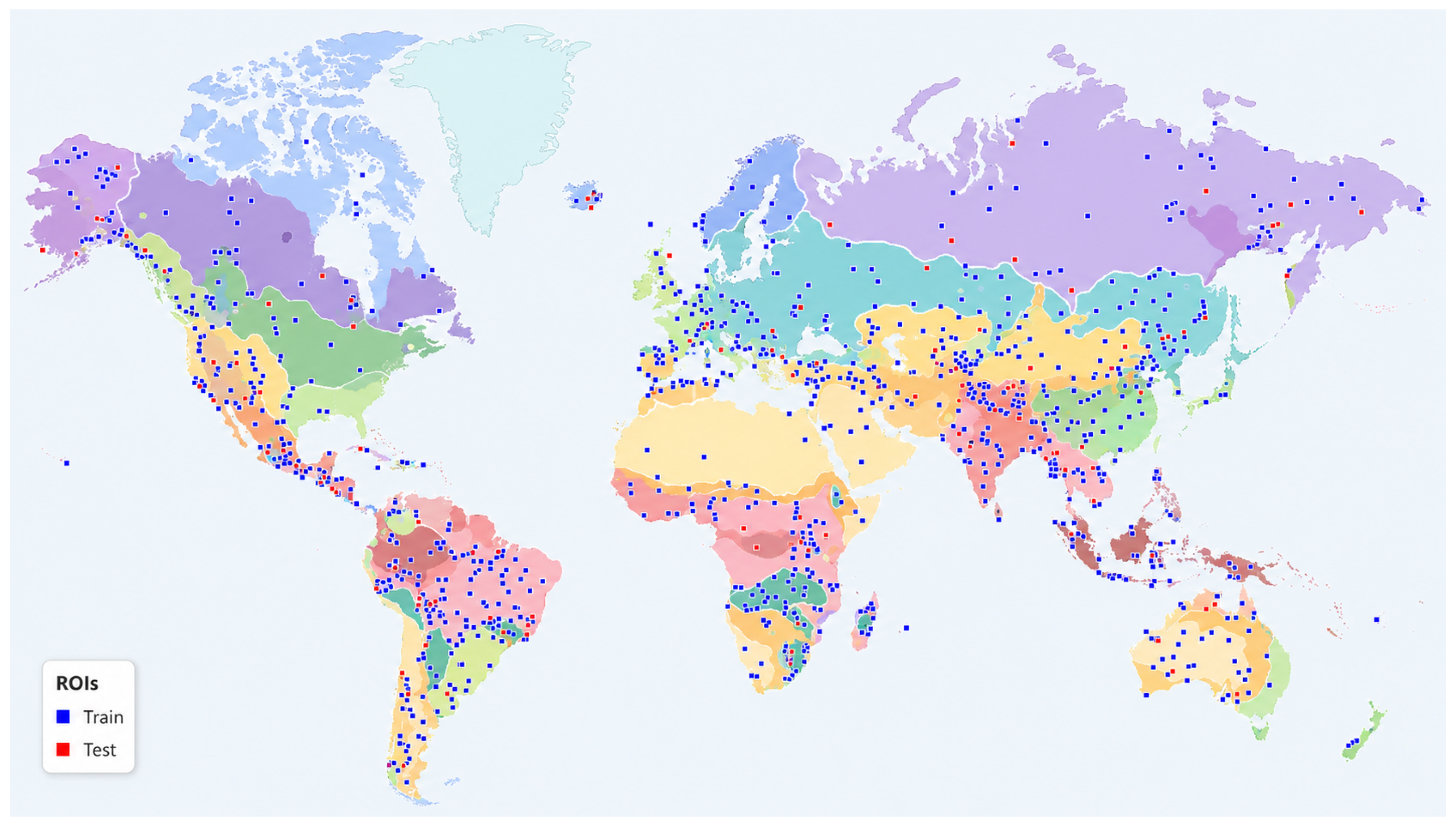
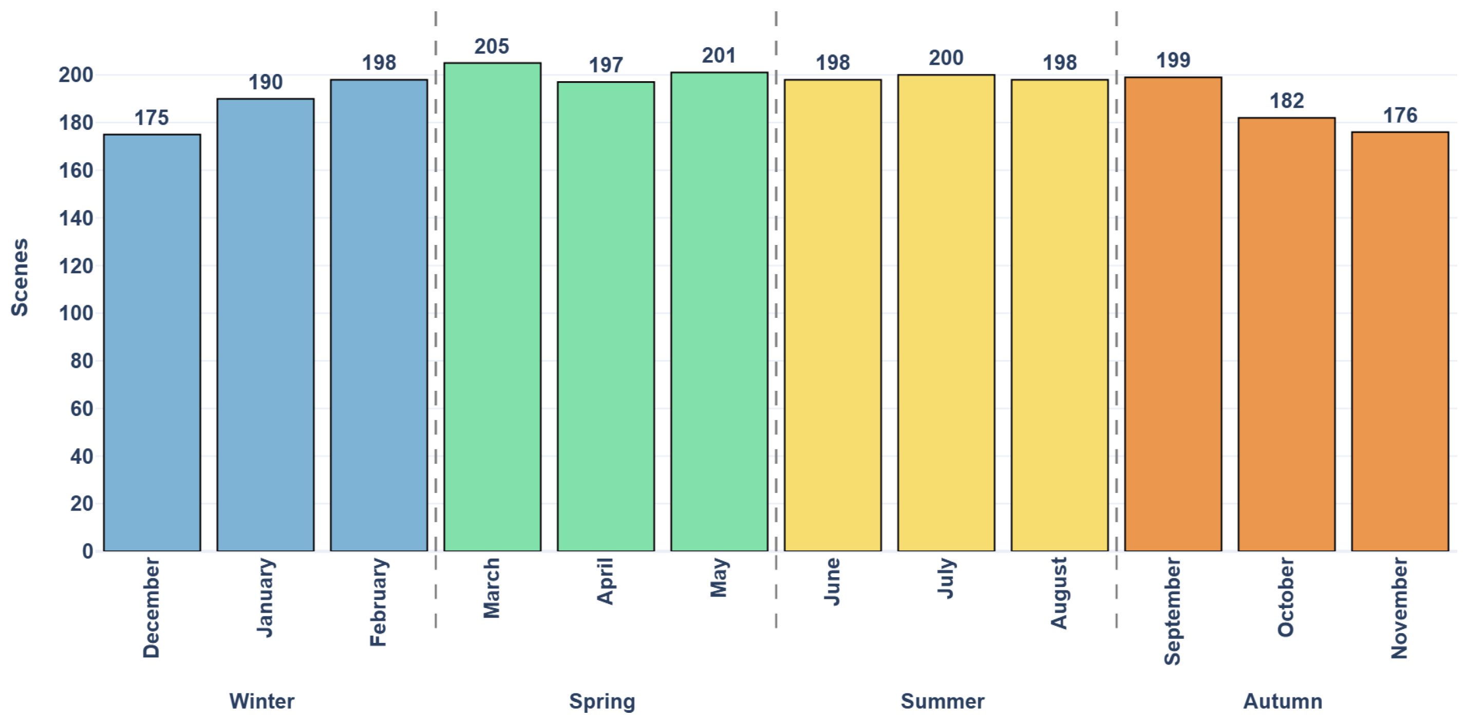
The dataset used in our experiments is SEN12TP [26,27]. It consists of 2321 globally distributed scenes (as visible in Figure 1), each covering an area of $20\times 20\mathrm{km}$. Each scene includes a near-synchronous paired Sentinel-1 and Sentinel-2 acquisition, together with a digital elevation model (DEM) and a land-cover map. The dataset was selected because the short temporal gap between radar and optical observations reduces cross-sensor decorrelation, which is particularly important for image translation and regression tasks. Moreover, as Figure 2 shows, the acquisitions cover all the seasonal variability and their numbers are balanced in all the periods, making it a perfect dataset to build generalized methods.

The Sentinel-1 Ground Range Detected (GRD) data correspond to orthorectified and radiometrically corrected SAR backscatter imagery with a spatial resolution of $10\times 10$ m. Five layers are provided: ${\sigma }_{VV}^0$, ${\sigma }_{VH}^0$, ${\gamma }_{VV}^0$, ${\gamma }_{VH}^0$, and $incAngle$. The variables ${\sigma }_{VV}^0$ and ${\sigma }_{VH}^0$ denote the backscatter coefficients for the VV and VH polarizations without radiometric terrain flattening, whereas ${\gamma }_{VV}^0$ and ${\gamma }_{VH}^0$ represent the terrain-flattened backscatter coefficients. The $incAngle$ layer stores the local incidence angle.

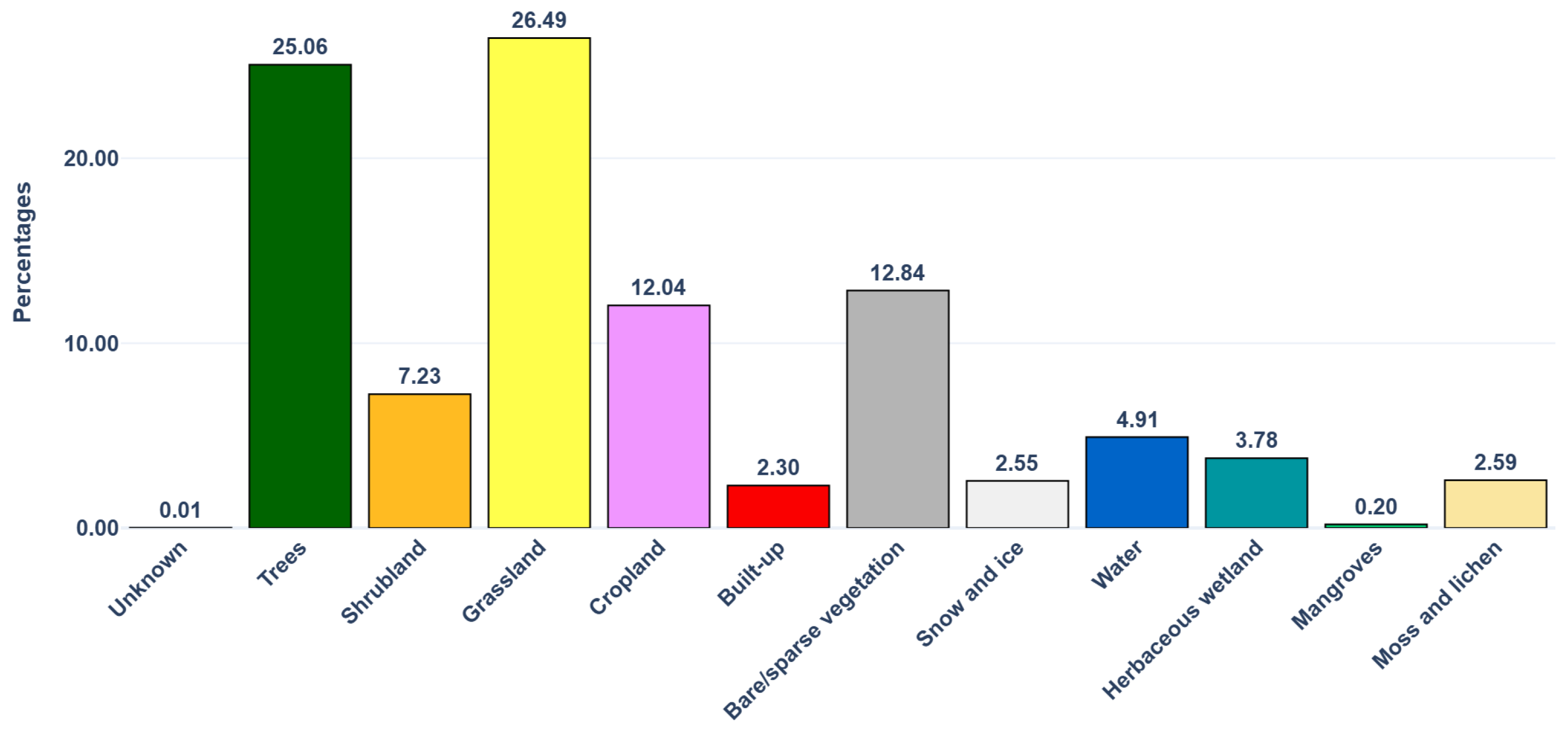
Sentinel-2 data provide multispectral optical information and include the following bands and auxiliary layer: b1 (aerosol), b2 (blue), b3 (green), b4 (red), b5 (red edge), b6 (red edge), b7 (red edge), b8 (NIR), b8A, b9, b10, b11 (SWIR), b12 (SWIR), and $cloud\_probability$. The optical data are provided at 10 m spatial resolution. The DEM is derived from ALOS World 3D and has a native spatial resolution of 30 m and gives information about the height of the surface and general structure. Finally, the land-cover layer is obtained from ESA WorldCover [30,31,32] at 10 m resolution and maps the selected areas into 10 different semantic classes, including Tree cover, Shrubland, Grassland, Cropland, Built-up, Bare/sparse vegetation, Snow and ice, Water, Herbaceous wetland, Mangroves, and Moss and lichen. Figure 3 reports the distribution of the land-cover classes in terms of percentage.

In our experiments, Sentinel-1, the elevation layer, and WorldCover are used as inputs, while Sentinel-2 bands are used as targets. For the SAR component, we retain only the terrain-flattened backscatter coefficients ${\gamma }_{VV}^0$ and ${\gamma }_{VH}^0$, since they are less sensitive to topographic effects and local incidence angle variations, thus providing a more stable representation across different terrain conditions. The SAR component is already preprocessed by the original authors of SEN12TP [26,27]. The preprocessing procedure, as described by the Google Earth Engine documentation https://developers.google.com/earth-engine/guides/sentinel1 (accessed on 13 July 2026), includes applying the orbit file, GRD border noise removal, thermal noise removal, and radiometric calibration. A radiometric terrain correction (RTC) [33], using volume scattering on the ground for the model optimization [34], is also applied to counter the negative impact that the terrain correction and orthorectification can have on the relation between SAR and NDVI. No additional speckle filtering was applied by the authors beyond the preprocessing already included in the SEN12TP product. For the optical targets, we exclude bands b1, b8A, b9, and b10, and reconstruct the remaining bands: b2, b3, b4, b5, b6, b7, b8, b11, and b12. These bands contain the spectral information required to compute most vegetation and soil indices considered in this study.

4. Methodology

4.1. General Pipeline

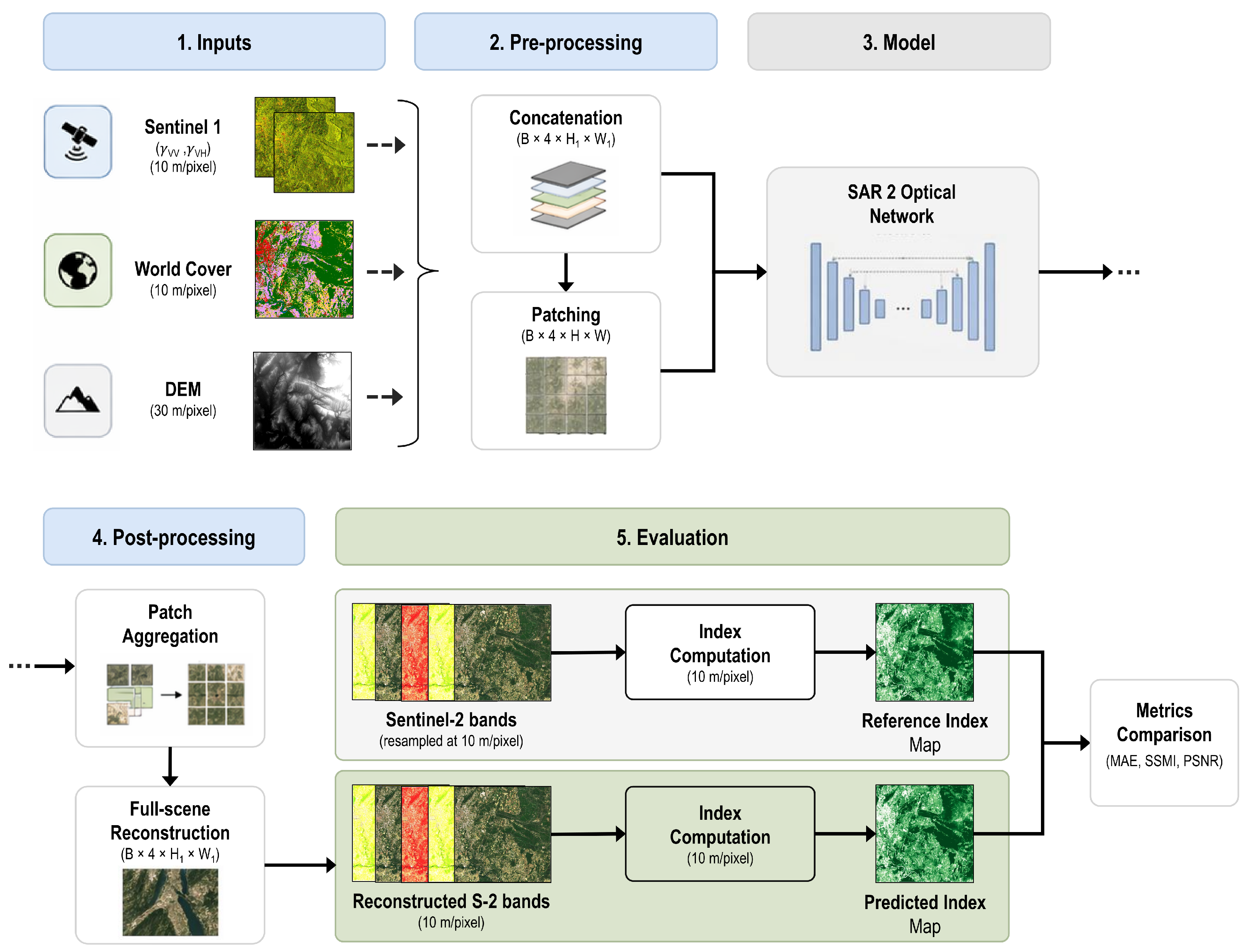
This section describes the general methodology adopted in our experiments, independently of the specific architectural and training choices. The considered architectures and optimization strategies are detailed in Section 4.2. An overview of the complete workflow is reported in Figure 4.

The objective of this study is twofold. First, we investigate the reconstruction of Sentinel-2 multispectral bands from SAR observations and auxiliary information. Second, we evaluate whether the reconstructed spectral information can be effectively used to derive vegetation and soil indices, comparing this strategy against the standard direct SAR-to-index formulation.

Both approaches share the same multimodal input configuration. Each scene includes Sentinel-1 SAR backscatter coefficients (VV and VH polarizations), ESA WorldCover semantic labels, and a digital elevation model (DEM). These heterogeneous sources are integrated through an early-fusion strategy. In particular, all modalities are spatially aligned and resampled to a common spatial resolution of 10 m/pixel when necessary, and subsequently concatenated into a unified input tensor.

For model training and patch-level validation/testing, each scene is partitioned into non-overlapping patches of size $H\times W$, with $H=W=128$. This non-overlapping patch-wise formulation reduces computational requirements, avoids redundant training samples, and enables efficient optimization on high-resolution scenes. The resulting patches correspond to four-channel tensors of spatial size $128\times 128$, which are then used as inputs to the neural networks.

Depending on the considered reconstruction strategy, the output layer of the network differs as follows:

• SAR-to-multispectral reconstruction: The network predicts nine Sentinel-2 spectral bands covering the visible, red edge, near-infrared, and short-wave infrared spectral regions, namely, blue (b2), green (b3), red (b4), red edge (b5, b6, b7), near infrared (b8), and short-wave infrared (b11, b12). The reconstructed multispectral outputs are subsequently used to derive the spectral indices considered in this study.
• SAR-to-index reconstruction: The network directly predicts a single target index. In this case, the model is trained separately for each index using the corresponding Sentinel-2-derived product as supervision.

The reconstructed multispectral bands are used to derive a set of spectral indices commonly adopted in Earth observation applications. In particular, we consider the Normalized Difference Vegetation Index (NDVI), the Green Normalized Difference Vegetation Index (GNDVI), the Normalized Difference Red Edge Index (NDRE), the Soil-Adjusted Vegetation Index (SAVI), the Normalized Difference Water Index (NDWI), the Bare Soil Index (BSI), and the Normalized Difference Snow Index (NDSI). For the direct SAR-to-index formulation, an independent model is trained for each target index. This distinction allows us to evaluate the trade-off between the flexibility of multispectral reconstruction and the specialization of direct index prediction.

For full-scene inference, the trained models are applied using an overlapping sliding-window strategy. Specifically, we use patches of size $128\times 128$ with a stride of 32 pixels, corresponding to a 75% overlap between adjacent patches in both spatial directions. At the image boundaries, the last patch is shifted when necessary to ensure complete coverage of the scene. The predicted patches are then reassembled to reconstruct the original full-scene products. To reduce boundary discontinuities and tiling artifacts introduced by the patch-wise processing, overlapping regions are merged through Gaussian-weighted blending. In this formulation, pixels closer to the patch center receive higher weights than those near the borders, resulting in smoother transitions between adjacent patches and improved spatial consistency in the reconstructed scenes.

4.2. Model Architectures

This section describes the neural architectures adopted for SAR-to-multispectral reconstruction. In particular, we compare three different paradigms: a deterministic Efficient-UNet, an adversarial Pix2Pix framework, and a conditional flow matching model based on a UNet backbone.

4.2.1. Efficient-UNet

The Efficient-UNet is a U-shaped network with EfficientNet [35] as the encoder. The encoder, including the bottleneck, is composed of 17 Mobile Inverted Bottleneck Convolution (MBConv) layers, which represent the core building block of EfficientNet [35]. The decoder consists of five deconvolutional layers connected to the encoder through skip connections. The final decoder layer predicts the nine Sentinel-2 surface reflectance bands. The model is trained in a supervised setting using Sentinel-2 multispectral images or indices as ground-truth targets. The reconstruction objective is defined separately for each translation paradigm, spectral band translation (SAR-to-multispectral) and vegetation index translation (SAR-to-index), as the two tasks differ in their outputs. In the SAR-to-multispectral setting, the model predicts nine Sentinel-2 surrogate spectral bands, whereas in the SAR-to-index setting it directly predicts a single Sentinel-2-derived index map. Accordingly, we adopt two task-specific loss functions.

For SAR-to-multispectral reconstruction, the training objective combines pixel-wise radiometric agreement ${\mathcal{L}}_{\mathrm{L}1}^{\mathrm{MS}}$, perceptual consistency ${\mathcal{L}}_{\mathrm{VGG}}$, and spectral fidelity ${\mathcal{L}}_{\mathrm{SAM}}$:

$${\mathcal{L}}_{\mathrm{MS}}={\alpha }_{\mathrm{MS}}{\mathcal{L}}_{\mathrm{L}1}^{\mathrm{MS}}+{\beta }_{\mathrm{MS}}{\mathcal{L}}_{\mathrm{VGG}}+{\gamma }_{\mathrm{MS}}{\mathcal{L}}_{\mathrm{SAM}},$$

(1)

where ${\alpha }_{\mathrm{MS}}$, ${\beta }_{\mathrm{MS}}$, and ${\gamma }_{\mathrm{MS}}$ are non-negative weighting coefficients.

The three components of Equation (1) are defined with respect to the multimodal input patch $\mathbf{x}$, the target Sentinel-2 multispectral patch $\mathbf{y}$, and the corresponding network prediction $\widehat{\mathbf{y}}=G\left(\mathbf{x}\right)$. The L1 term measures the average pixel-wise radiometric discrepancy between predicted and reference bands:

$${\mathcal{L}}_{\mathrm{L}1}^{\mathrm{MS}}={\mathbb{E}}_{(\mathbf{x},\mathbf{y})}\left[{∥\widehat{\mathbf{y}}-\mathbf{y}∥}_1\right].$$

(2)

To complement this pixel-wise constraint with a higher-level spatial representation, the perceptual term is computed on a false-color RGNIR image built from Sentinel-2 bands b8, b4, and b3:

$${\mathcal{L}}_{\mathrm{VGG}}={\mathbb{E}}_{(\mathbf{x},\mathbf{y})}\left[{∥{\mathbf{F}}^{\left(4\right)}\left({\widehat{\mathbf{y}}}_{\mathrm{RGNIR}}\right)-{\mathbf{F}}^{\left(4\right)}\left({\mathbf{y}}_{\mathrm{RGNIR}}\right)∥}_1\right],$$

(3)

where ${\mathbf{F}}^{\left(4\right)}(·)$ denotes the feature map extracted from the fourth convolutional block of a VGG16 network pre-trained on natural images. Finally, spectral consistency across the reconstructed bands is encouraged through the Spectral Angle Mapper loss:

$${\mathcal{L}}_{\mathrm{SAM}}={\displaystyle \frac{1}{HW}}{\displaystyle \sum _{i=1}^{HW}}arccos\left({\displaystyle \frac{{\widehat{\mathbf{y}}}_i·{\mathbf{y}}_i}{{\parallel {\widehat{\mathbf{y}}}_i\parallel }_2{\parallel {\mathbf{y}}_i\parallel }_2}}\right),$$

(4)

where H and W are the patch height and width, and ${\widehat{\mathbf{y}}}_i$ and ${\mathbf{y}}_i$ are the predicted and reference spectral vectors at pixel i.

For direct SAR-to-index reconstruction, the network predicts one Sentinel-2-derived index map at a time rather than a full multispectral image. Since the target is a single-index product, the VGG and SAM terms used for multispectral reconstruction are replaced by domain-oriented structural terms that do not rely on RGB-like representations or ImageNet-derived features. The adopted objective combines pixel-wise index agreement, multi-scale edge preservation, and structural similarity:

$${\mathcal{L}}_{\mathrm{IDX}}={\alpha }_{\mathrm{IDX}}{\mathcal{L}}_{\mathrm{L}1}^{\mathrm{IDX}}+{\beta }_{\mathrm{IDX}}{\mathcal{L}}_{\mathrm{MS-Grad}}+{\gamma }_{\mathrm{IDX}}{\mathcal{L}}_{\mathrm{SSIM}},$$

(5)

where ${\alpha }_{\mathrm{IDX}}$, ${\beta }_{\mathrm{IDX}}$, and ${\gamma }_{\mathrm{IDX}}$ are non-negative weighting coefficients controlling the contribution of the three terms. As for the multispectral objective, these coefficients were selected empirically over alternative parameter combinations.

The three components of Equation (5) are defined with respect to the multimodal input patch $\mathbf{x}$, the target Sentinel-2-derived index patch $\mathbf{z}$, and the corresponding network prediction $\widehat{\mathbf{z}}=G\left(\mathbf{x}\right)$. The L1 term measures the average pixel-wise discrepancy between the predicted and reference index values:

$${\mathcal{L}}_{\mathrm{L}1}^{\mathrm{IDX}}={\mathbb{E}}_{(\mathbf{x},\mathbf{z})}\left[{∥\widehat{\mathbf{z}}-\mathbf{z}∥}_1\right].$$

(6)

To better preserve local spatial variations, boundaries, and fine-scale structures in the index maps, we include a multi-scale gradient loss:

$${\mathcal{L}}_{\mathrm{MS-Grad}}={\mathbb{E}}_{(\mathbf{x},\mathbf{z})}\left[{\displaystyle \frac{1}{{\sum }_s{w}_s}}{\displaystyle \sum _{s=0}^{S-1}}{w}_s{\mathcal{L}}_{\mathrm{Grad}}\left({\widehat{\mathbf{z}}}^{\left(s\right)},{\mathbf{z}}^{\left(s\right)}\right)\right],w_s={\displaystyle \frac{1}{2^s}},$$

(7)

where ${\widehat{\mathbf{z}}}^{\left(s\right)}$ and ${\mathbf{z}}^{\left(s\right)}$ are obtained by downsampling the predicted and target index maps s times by average pooling. At each scale, the gradient loss compares finite differences along the horizontal and vertical directions:

$${\mathcal{L}}_{\mathrm{Grad}}(\widehat{\mathbf{z}},\mathbf{z})={∥{\partial }_x\widehat{\mathbf{z}}-{\partial }_x\mathbf{z}∥}_1+{∥{\partial }_y\widehat{\mathbf{z}}-{\partial }_y\mathbf{z}∥}_1,$$

(8)

with ${\partial }_x{f}_{h,w}=f_{h,w+1}-f_{h,w}$ and ${\partial }_y{f}_{h,w}=f_{h+1,w}-f_{h,w}$. Finally, local structural consistency is encouraged through an SSIM-based loss:

$${\mathcal{L}}_{\mathrm{SSIM}}={\mathbb{E}}_{(\mathbf{x},\mathbf{z})}\left[1-\mathrm{SSIM}(\widehat{\mathbf{z}},\mathbf{z})\right],$$

(9)

where the SSIM map is computed using Gaussian-windowed local statistics with window size $k=11$ and $\sigma =1.5$. The stability constants are $C_1={\left(K_{1}L\right)}^2$ and $C_2={\left(K_{2}L\right)}^2$, with $K_1=0.01$ and $K_2=0.03$.

The influence of ${\alpha }_{\mathrm{MS}}$, ${\beta }_{\mathrm{MS}}$, and ${\gamma }_{\mathrm{MS}}$ on the reconstruction performance was evaluated through an ablation study over alternative parameter combinations. To determine the weighting coefficients of the multispectral reconstruction loss, we first performed a preliminary binary ablation on the loss components. This analysis showed that the pixel-wise $L_1$ term should always be retained as the main reconstruction constraint, whereas the perceptual and spectral-consistency terms are more effective as auxiliary regularizers. Based on this observation, we fixed ${\alpha }_{MS}=1$ and performed a grid search over ${\beta }_{MS}$ and ${\gamma }_{MS}$ in the set $\{0,0.01,0.05,0.1,0.5,1,2,5\}$. Model selection was carried out on the validation set using a composite score obtained from the normalized MAE, PSNR, and SSIM values, with error-based metrics inverted so that higher scores consistently indicated better performance. The best configuration was obtained for ${\beta }_{MS}=0.01$ and ${\gamma }_{MS}=0.05$, and these values were adopted in all subsequent multispectral reconstruction experiments.

The implementation of the network architectures was based on the segmentation_models.pytorch library (https://github.com/qubvel-org/segmentation_models.pytorch, accessed on 13 July 2026). EfficientNet-B0 was selected as the encoder backbone to provide a compromise between computational efficiency and reconstruction performance.

4.2.2. Pix2Pix

Pix2Pix is a conditional generative adversarial framework designed for paired image-to-image translation [36]. Unlike the deterministic Efficient-UNet, this approach relies on two jointly trained neural networks: a generator $\mathbf{G}$ that maps SAR inputs to multispectral outputs, and a discriminator $\mathbf{D}$ that enforces local realism and input consistency.

The generator follows a standard U-Net encoder–decoder architecture with skip connections. At the same time, the discriminator adopts a PatchGAN formulation [36], which evaluates the realism of local image patches rather than producing a single global classification output.

Given the conditioning input $\mathbf{x}$ and either the real target $\mathbf{y}$ or the generated output $\widehat{\mathbf{y}}$, the discriminator processes their channel-wise concatenation and produces a spatial probability map indicating the likelihood that each local patch corresponds to a real multispectral observation.

The two networks are jointly optimized through a combination of adversarial and reconstruction losses. As a reconstruction objective, we adopt the same three-component loss introduced in Equations (1) and (5). The adversarial component corresponds to the discriminator objective:

$${\mathcal{L}}_{\mathrm{ADV}}={\mathbb{E}}_{\mathbf{x},\mathbf{y}}\left[\log \mathbf{D}(\mathbf{x},\mathbf{y})\right]+{\mathbb{E}}_{\mathbf{x}}\left[\log (1-\mathbf{D}(\mathbf{x},\mathbf{G}\left(\mathbf{x}\right)))\right].$$

(10)

The generator is instead trained using the combined objective:

$${\mathcal{L}}_{GEN}={\mathcal{L}}_{\mathrm{ADV}}+{\lambda }_{\mathrm{rec}}{\mathcal{L}}_{\mathrm{REC}}.$$

(11)

where ${\lambda }_{\mathrm{rec}}=100$, following the standard Pix2Pix configuration.

4.2.3. Conditional Flow Matching

Flow matching is a generative modeling framework based on continuous normalizing flows, where the objective is to learn a deterministic transformation between a simple probability distribution and a complex target distribution [37].

In this work, we adopt the image conditional flow matching paradigm proposed by Tong et al. [38]. The conditioning input corresponds to the four-channel tensor $\mathbf{x}$, composed of SAR backscatter, elevation, and WorldCover information, while the target distribution corresponds to the nine-channel Sentinel-2 multispectral reflectance tensor.

Unlike the previously discussed approaches, flow matching does not directly learn a deterministic mapping between $\mathbf{x}$ and the target image ${\mathbf{y}}_0$. Instead, the model learns a conditioned time-dependent velocity field:

$${\displaystyle \frac{d\mathbf{y}}{dt}}=v_{\theta }(\mathbf{y}\left(t\right),t\mid \mathbf{x})$$

(12)

where $\mathbf{y}\left(t\right)$ follows a linear interpolation path between the target sample ${\mathbf{y}}_0$ and a Gaussian noise realization ${\mathbf{y}}_1\sim \mathcal{N}(0,\mathbf{I})$:

$$\mathbf{y}\left(t\right)=(1-t){\mathbf{y}}_0+t{\mathbf{y}}_1$$

(13)

The velocity field $v_{\theta }$ is parameterized using a depth-two UNet conditioned on both the auxiliary inputs and temporal embeddings. The network receives as input the noisy sample $\mathbf{y}\left(t\right)$, the conditioning tensor $\mathbf{x}$, and a sinusoidal temporal embedding vector.

Conditioning is introduced through channel-wise concatenation at multiple resolution levels of the network. During encoding, both the feature maps and the conditioning inputs are progressively downsampled while preserving spatial alignment. In the decoding stage, conditioning information is upsampled and combined with encoder skip connections to preserve fine-scale spatial details. Temporal embeddings are injected through feature-wise modulation mechanisms.

The model is trained using the flow matching objective [37], corresponding to an ${\ell }_2$ loss between the predicted velocity field and the target interpolation direction $({\mathbf{y}}_1-{\mathbf{y}}_0)$. At each training iteration, a timestep t is sampled uniformly in $[0,1]$, and the model learns to predict a consistent denoising direction regardless of the considered noise level.

4.3. Training Details

All models are implemented in PyTorch 2.12.1+cu126 and trained using the Adam optimizer. For Efficient-UNet and conditional flow matching, the learning rate is set to ${10}^{-4}$, whereas Pix2Pix adopts a learning rate of $2\times {10}^{-4}$ with momentum parameters $({\beta }_1,{\beta }_2)=(0.5,0.999)$, following the original implementation [36]. It should be noted that the overlapping sliding-window strategy is used only during full-scene inference and aggregation, whereas the training patches are extracted without overlap.

Gradient clipping is applied during training to improve optimization stability. Early stopping is adopted in all experiments based on validation performance in order to reduce overfitting. Unless otherwise specified, training is performed on patches of size $128\times 128$.

For the conditional flow matching model, inference is performed through numerical integration of the learned velocity field using 50 timesteps.

Finally, the dataset is split into train, validation, and test. In particular, the original split is adopted, with a ratio of 80/10/10 for training, validation, and test, respectively.

4.4. Evaluation Metrics

To evaluate the quality of the reconstructed multispectral bands and derived spectral indices, we adopt three complementary metrics commonly used in image reconstruction and translation tasks: mean absolute error (MAE), peak signal-to-noise ratio (PSNR), and structural similarity index measure (SSIM).

MAE (Equation (14)) measures the average pixel-wise absolute difference between the reference image y and the reconstructed output $\widehat{y}$:

$$\mathrm{MAE}={\displaystyle \frac{1}{n}}{\displaystyle \sum _{i=1}^n}\left|y_i-{\widehat{y}}_i\right|$$

(14)

where n denotes the total number of pixels. This metric provides a direct estimate of reconstruction accuracy at the pixel level, although it does not explicitly account for structural or perceptual consistency.

PSNR (Equation (15)) evaluates the reconstruction fidelity in terms of the logarithmic signal-to-noise ratio:

$$\mathrm{PSNR}=10{log}_{10}\left({\displaystyle \frac{{\mathrm{MAX}}^2}{\mathrm{MSE}}}\right)$$

(15)

where $MAX$ is the maximum possible pixel value and MSE denotes the mean squared error between the reconstructed and reference images. Higher PSNR values indicate improved reconstruction quality.

SSIM (Equation (16)) measures perceptual similarity by jointly considering luminance, contrast, and structural consistency between the reconstructed and reference images:

$$\mathrm{SSIM}(x,y)={\displaystyle \frac{(2{\mu }_x{\mu }_y+C_1)(2{\sigma }_{xy}+C_2)}{({\mu }_x^2+{\mu }_y^2+C_1)({\sigma }_x^2+{\sigma }_y^2+C_2)}}$$

(16)

where ${\mu }_x$ and ${\mu }_y$ are the mean intensities, ${\sigma }_x^2$ and ${\sigma }_y^2$ denote the variances, and ${\sigma }_{xy}$ is the covariance between the two images. The constants $C_1$ and $C_2$ are introduced to improve numerical stability. In particular, $C_1={\left(k_{1}L\right)}^2$ and $C_2={\left(k_{2}L\right)}^2$, where $k_1=0.01$, $k_2=0.03$, and L represents the dynamic range of the pixel values. In our experiments, all spectral bands are normalized within the $[0,1]$ interval, therefore $L=1$.

All metrics are computed both on reconstructed spectral bands and on the derived spectral index maps.

In addition, to evaluate the reconstruction of the spectral bands, we also adopt Spectral Angle Mapper (SAM), which gives us a general overview of the entire reconstruction of the spectral signal, considering the entire spectrum at the same time.

SAM (Equation (17)) is usually used in remote sensing and image processing to determine the spectral similarity between two spectra and is computed as follows:

$$\mathrm{SAM}={\displaystyle \frac{1}{n}}{\displaystyle \sum _{i=1}^n}arccos\left({\displaystyle \frac{y_i·\widehat{y_i}}{\parallel y_i\parallel \parallel \widehat{y_i}\parallel }}\right)$$

(17)

where $y_i$ and $\widehat{y_i}$ are corresponding pixels in the reference image and reconstructed image, respectively, and n is the total number of pixels. Even with this metric, the achieved results are to be read as the lower the better.

5. Results and Discussion

In this section, we first present the results achieved in spectral band reconstruction and, second, compare the two approaches for estimating vegetation indices. The first investigation considers the methodology described in the previous section, while the second considers the best approach of the first analysis and reports the results of this architecture on the direct estimation of the indices and from the inference of the spectral bands.

5.1. Band Reconstruction

The first analysis compares the three different deep learning approaches for spectral-band reconstruction. Efficient-UNet, Pix2Pix, and flow matching are compared both in terms of metric performance (with MAE, PSNR, and SSIM) and from a qualitative/visual point of view.

5.1.1. Performance Overview

Table 2. Quantitative comparison of the SAR-to-multispectral reconstruction approaches. Lower MAE and higher PSNR/SSIM indicate better reconstruction quality.

Metric	Band	Efficient-UNet	Pix2Pix	Flow Matching
MAE ↓	Blue (b2)	0.072 ± 0.106	0.079 ± 0.100	0.125 ± 0.156
	Green (b3)	0.075 ± 0.103	0.082 ± 0.097	0.124 ± 0.148
	Red (b4)	0.081 ± 0.101	0.087 ± 0.095	0.130 ± 0.144
	Red edge (b5)	0.082 ± 0.100	0.089 ± 0.094	0.128 ± 0.141
	Red edge (b6)	0.090 ± 0.091	0.098 ± 0.085	0.137 ± 0.125
	Red edge (b7)	0.093 ± 0.085	0.100 ± 0.079	0.140 ± 0.114
	NIR (b8)	0.096 ± 0.087	0.104 ± 0.083	0.144 ± 0.115
	SWIR (b11)	0.055 ± 0.027	0.063 ± 0.030	0.087 ± 0.036
	SWIR (b12)	0.047 ± 0.026	0.055 ± 0.028	0.075 ± 0.034
	Overall	0.077 ± 0.081	0.084 ± 0.077	0.121 ± 0.108
PSNR ↑	Blue (b2)	25.341 ± 9.566	24.002 ± 9.643	17.897 ± 6.978
	Green (b3)	24.465 ± 8.973	23.220 ± 9.030	18.041 ± 6.740
	Red (b4)	23.199 ± 8.279	22.032 ± 8.149	17.543 ± 6.327
	Red edge (b5)	22.968 ± 7.923	21.774 ± 7.831	17.663 ± 6.211
	Red edge (b6)	21.205 ± 6.247	19.947 ± 6.095	16.838 ± 5.084
	Red edge (b7)	20.582 ± 5.675	19.530 ± 5.556	16.434 ± 4.526
	NIR (b8)	20.189 ± 5.597	19.134 ± 5.489	16.110 ± 4.464
	SWIR (b11)	23.773 ± 3.749	22.530 ± 3.748	19.684 ± 3.100
	SWIR (b12)	25.127 ± 4.172	23.788 ± 4.002	20.975 ± 3.452
	Overall	22.983 ± 6.687	21.773 ± 6.616	17.909 ± 4.875
SSIM ↑	Blue (b2)	0.707 ± 0.238	0.646 ± 0.255	0.530 ± 0.236
	Green (b3)	0.703 ± 0.233	0.643 ± 0.254	0.529 ± 0.232
	Red (b4)	0.657 ± 0.215	0.590 ± 0.232	0.459 ± 0.199
	Red edge (b5)	0.694 ± 0.211	0.623 ± 0.228	0.523 ± 0.207
	Red edge (b6)	0.631 ± 0.192	0.527 ± 0.191	0.439 ± 0.157
	Red edge (b7)	0.608 ± 0.183	0.508 ± 0.184	0.408 ± 0.142
	NIR (b8)	0.542 ± 0.184	0.446 ± 0.180	0.338 ± 0.128
	SWIR (b11)	0.722 ± 0.120	0.601 ± 0.186	0.529 ± 0.130
	SWIR (b12)	0.745 ± 0.112	0.623 ± 0.192	0.551 ± 0.130
	Overall	0.668 ± 0.188	0.579 ± 0.211	0.478 ± 0.160

reports the quantitative results achieved by the SAR-to-multispectral reconstruction models considered. Overall, all methods exhibit consistent reconstruction trends across spectral bands, suggesting that reconstruction difficulty is primarily driven by the intrinsic spectral characteristics of each band rather than by the specific modeling strategy.

Among the evaluated approaches, Efficient-UNet achieves the best overall performance across all evaluation metrics, consistently outperforming Pix2Pix and flow matching in terms of MAE, PSNR, and SSIM. Even considering SAM on the entire spectral reconstruction. Efficient-UNet achieves an SAM of $0.155\pm 0.081$, while Pix2Pix achieves $0.187\pm 0.089$ and flow matching $0.269\pm 0.010$, corroborating the conclusion that, among them, Efficient-UNet is the best-performing. To assess the statistical reliability of the reported differences, we applied Welch’s two-sample t-tests to all pairwise comparisons, using the reported means and standard deviations as population proxies over the $n=232$ test samples. The statistical tests were conducted using per-scene metric values as the sample units, since each scene represents statistically independent observations. The Welch’s two-sample t-test was preferred over the standard Student’s t-test as it does not assume equal variances between the two compared models. For MAE, the advantage of Efficient-UNet over Pix2Pix is not statistically significant for most spectral bands ($p>0.10$), with the exception of SWIR (b11) and SWIR (b12), where a small but significant effect is observable ($p=0.003$ and $p=0.002$, respectively). The overall MAE gap is also non-significant ($p=0.34$), confirming that the two models produce comparable pixel-wise absolute errors across the majority of the spectrum. For PSNR, Efficient-UNet achieves a statistically significant advantage only on the spectrally challenging bands, red edge ($p=0.029$ for b6, and $p=0.044$ for b7), NIR ($p=0.041$), and SWIR ($p<0.001$), while no significant differences emerge for the visible bands (b2, b3, b4) and red edge (b5) ($p>0.10$), and the overall PSNR gap just misses the conventional significance threshold ($p=0.05$). This suggests that the signal-to-noise advantage of Efficient-UNet is concentrated in the longer-wavelength bands rather than being a widespread phenomenon. For SSIM, Efficient-UNet significantly outperforms Pix2Pix across all bands (with $p<0.01$ in all cases and, in more detail, $p<0.001$ for the red edge, NIR, and both SWIR bands), indicating it consistently produces structurally less faithful reconstructions despite the comparable pixel-wise error observed in MAE. Regarding flow matching and Efficient-UNet, the latter is significantly superior across all bands and all metrics, with all p-values below $0.0001$, and no band or metric representing an exception. This confirms a consistent and robust advantage of Efficient-UNet over flow matching across the full spectral range.

A band-wise analysis reveals that the reconstruction difficulty strongly depends on the spectral region. In particular, the red edge (b6 and b7) and NIR (b8) bands represent the most challenging channels to reconstruct, whereas the visible and SWIR (b11 and b12) bands achieve comparatively higher reconstruction fidelity.

The SWIR (b11 and b12) bands consistently achieve the best reconstruction results across all metrics. This behavior can be partially explained by the stronger sensitivity of SAR backscatter to structural- and moisture-related properties that are also reflected within the SWIR spectral region.

Conversely, the NIR (b8) and red edge bands are strongly influenced by vegetation biochemical properties, including chlorophyll content and canopy structure, which are only indirectly observable through SAR measurements. As a consequence, the relationship between radar backscatter and these spectral responses is weak, indirect, highly nonlinear, and scene-dependent, leading to lower reconstruction accuracy and larger variability for b6, b7, and b8.

In more detail, SAR backscatter depends mostly on surface roughness and the dielectric properties, and thus on the moisture content in both soil and vegetation [39,40]. On the other hand, the red edge bands are sensitive to chlorophyll concentration and subtle pigment changes [41,42], while NIR (b8) is shaped by internal leaf structure and dry matter content rather than water content [43,44]. Therefore, the model must infer band values from the SAR input that actually have a weak and indirect physical correlation with each other, possibly causing the higher error and larger standard deviations observed.

The visible bands achieve comparatively high PSNR and SSIM values, indicating that the models are generally able to preserve the large-scale spatial organization of the scene. Nevertheless, the corresponding MAE values suggest residual inaccuracies in spectral reconstruction. This behavior is coherent with the nature of SAR observations, which are primarily sensitive to geometric structure and surface roughness rather than to chromatic reflectance properties. Consequently, the reconstructed visible bands tend to preserve spatial organization more effectively than precise spectral appearance.

5.1.2. Visual Overview

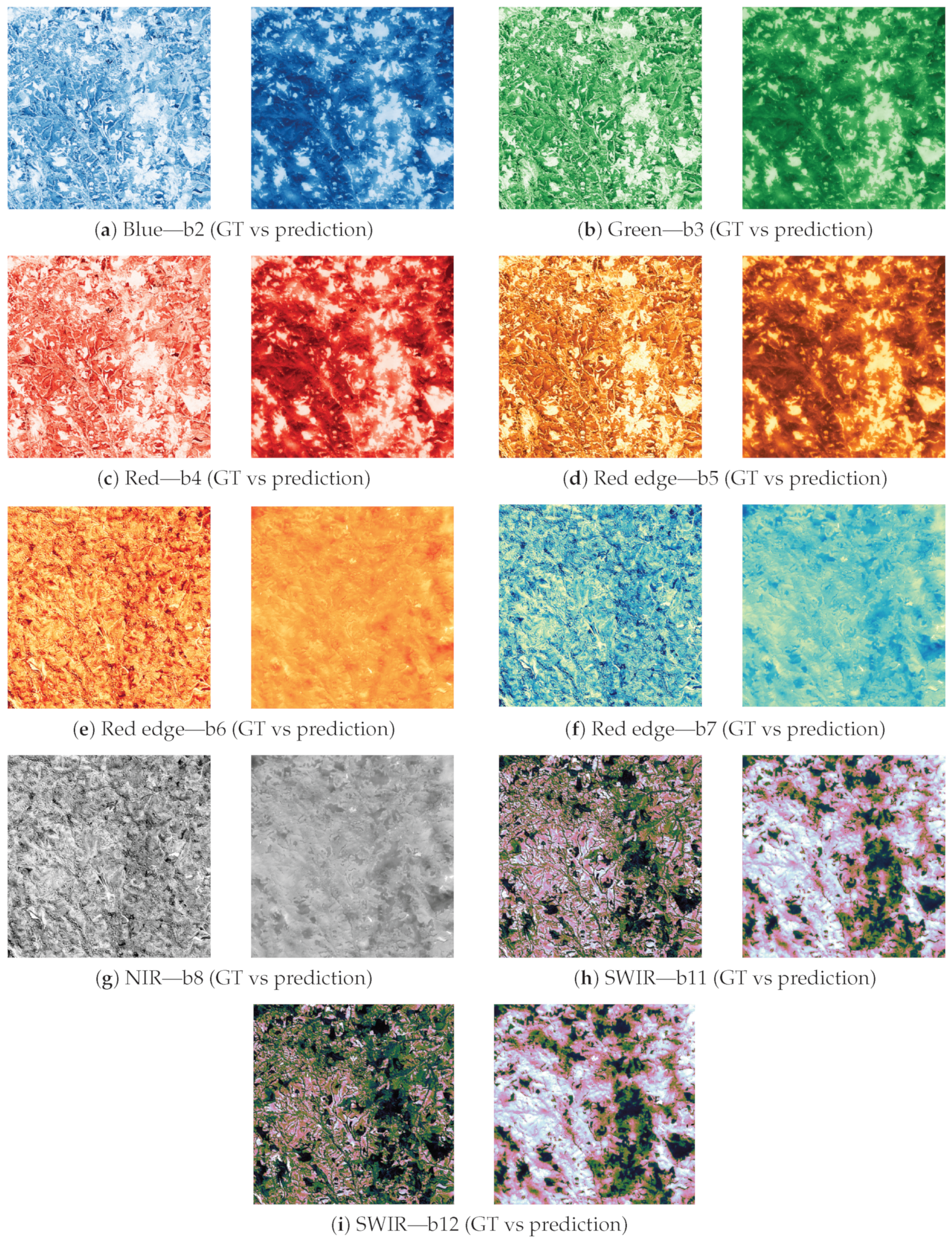
Figure 5 qualitatively confirms the quantitative evaluation reported in Table 2. For each band, the left image corresponds to the Sentinel-2 reference observation and the right image to the reconstructed output generated by Efficient-UNet. The qualitative results were obtained using the Efficient-UNet architecture, which achieved the best overall quantitative performance among the evaluated approaches.

The reconstructed bands preserve the global spatial organization of the scenes, including large homogeneous regions and major structural transitions. However, fine spatial details and localized spectral variations remain more difficult to recover, particularly in vegetation-sensitive regions. Although the reconstructed bands remain visually coherent with the corresponding Sentinel-2 targets, some smoothing effects are still observable around sharp transitions and high-frequency spatial structures. This behavior is consistent with the quantitative analysis, where the visible and SWIR bands exhibit comparatively higher reconstruction fidelity than the red edge and NIR channels.

5.2. Index Reconstruction

In this section, we compare two alternative strategies for spectral index estimation from SAR observations. The first strategy corresponds to direct index reconstruction through dedicated index-specific models, similarly to previous state-of-the-art approaches [27]. The second strategy derives the indices from the reconstructed multispectral bands generated by the SAR-to-multispectral framework proposed in this work. As a consequence of the previous investigation, for both the approaches the Efficient-UNet is considered as the deep learning framework.

The considered indices include the Bare Soil Index (BSI), Green Normalized Difference Vegetation Index (GNDVI), Normalized Difference Red Edge (NDRE), Normalized Difference Snow Index (NDSI), Normalized Difference Vegetation Index (NDVI), Normalized Difference Water Index (NDWI), and Soil-Adjusted Vegetation Index (SAVI).

5.2.1. Performance Overview

Table 3. Quantitative comparison between direct SAR-to-index reconstruction (custom model) and index derivation from reconstructed multispectral bands (inferred bands). Lower MAE and higher PSNR/SSIM indicate better reconstruction quality.

Metric	Index	Custom Model	Inferred Bands	$\Delta$
MAE ↓	BSI	0.100 ± 0.057	0.100 ± 0.058	0.000
	GNDVI	0.094 ± 0.050	0.096 ± 0.051	−0.002
	NDRE	0.042 ± 0.019	0.042 ± 0.020	0.000
	NDSI	0.134 ± 0.131	0.139 ± 0.138	−0.005
	NDVI	0.102 ± 0.055	0.104 ± 0.053	−0.002
	NDWI	0.094 ± 0.050	0.096 ± 0.051	−0.002
	SAVI	0.066 ± 0.030	0.069 ± 0.030	−0.003
	Overall	0.090 ± 0.056	0.092 ± 0.057	−0.002
PSNR ↑	BSI	24.695 ± 4.529	24.700 ± 4.495	−0.005
	GNDVI	24.901 ± 4.226	24.672 ± 4.015	0.229
	NDRE	31.421 ± 4.087	31.395 ± 4.206	0.026
	NDSI	22.803 ± 6.146	22.512 ± 6.199	0.291
	NDVI	24.416 ± 4.751	24.166 ± 4.343	0.250
	NDWI	24.898 ± 4.225	24.672 ± 4.015	0.226
	SAVI	28.193 ± 4.136	27.901 ± 4.043	0.292
	Overall	25.904 ± 4.586	25.717 ± 4.474	0.187
SSIM ↑	BSI	0.522 ± 0.272	0.514 ± 0.276	0.008
	GNDVI	0.671 ± 0.190	0.648 ± 0.203	0.023
	NDRE	0.631 ± 0.186	0.622 ± 0.195	0.009
	NDSI	0.648 ± 0.205	0.633 ± 0.213	0.015
	NDVI	0.627 ± 0.177	0.602 ± 0.179	0.025
	NDWI	0.671 ± 0.190	0.648 ± 0.203	0.023
	SAVI	0.679 ± 0.161	0.656 ± 0.170	0.023
	Overall	0.636 ± 0.197	0.618 ± 0.206	0.018

reports a quantitative comparison between direct SAR-to-index reconstruction (custom models) and the proposed multispectral reconstruction strategy (inferred bands). The latter computes the indices from the multispectral Sentinel-2 bands reconstructed by the Efficient-UNet model.

Considering the NDVI reconstruction, the obtained performance is comparable with previous studies (MAE = 0.106, PSNR = 22.079, SSIM = 0.594) [27], supporting the validity of the proposed experimental setting and confirming the effectiveness of the adopted SAR-to-index reconstruction pipeline. Overall, direct index-specific models consistently achieve slightly better quantitative performance across all evaluation metrics. Nevertheless, the performance gap between the two strategies remains limited for all the considered indices. In particular, the average MAE difference is approximately $0.002$, while the average SSIM reduction remains below 0.018, indicating that the inferred multispectral bands preserve most of the structural and spectral information required for index computation. The largest performance differences are observed for NDRE, NDVI, and SAVI, especially in terms of PSNR. This behavior is coherent with the previous spectral-band analysis, where the NIR and red edge channels represent the most challenging bands to reconstruct. Since these indices strongly depend on vegetation-sensitive spectral regions, even small reconstruction inaccuracies may propagate and slightly degrade the final index estimation. This effect is particularly relevant for indices that explicitly use the NIR or red edge bands, such as NDVI, GNDVI, NDRE, and SAVI, whereas indices relying more on visible or SWIR information are comparatively less affected by the b6–b8 reconstruction errors.

Although the direct index-specific models consistently achieve better quantitative performance, the gap with respect to the multispectral reconstruction strategy remains relatively small across all evaluation metrics. This result is particularly relevant because the proposed multispectral formulation enables the simultaneous derivation of multiple spectral indices without requiring dedicated training for each target product. Statistical testing confirms that the performance gap between the custom model and the inferred approach is not statistically significant for MAE across any of the evaluated indices (all $p>0.28$), nor for PSNR (all $p>0.44$), nor for SSIM (all $p>0.13$). This implies that the two strategies are statistically indistinguishable across all metrics and all indices. Crucially, the absence of significant differences across all three metrics and all seven indices provides strong statistical support for the practical equivalence of the two reconstruction paradigms and reinforces the case for the proposed multispectral approach as a flexible and competitive alternative to dedicated index-specific models.

From an operational perspective, this substantially increases the flexibility of the framework, allowing the extraction of additional spectral indices without retraining specialized models. Therefore, the slight reduction in reconstruction accuracy is compensated by a significant gain in scalability, generalization capability, and practical usability for large-scale Earth observation applications. A model that can directly extract the spectral information from a type of data that is robust to weather and light variations, such as SAR, has different advantages. First of all, the acquisition does not depend on time, date, or weather conditions that characterize the area, making it easier to decide how, when, and where to acquire data, without constraints and allowing for continuous monitoring. At the same time, the capability of substituting spectral information can help in training other models where the optical data are essential, using synthetic data. In situations where acquisition is challenging, due to clouds or light conditions, and emergencies, such as natural disasters, it can help in faster responses, compensating for both the limited interpretability of SAR and the lack of spectral information. In general, a model of this kind can remove the direct dependence on multispectral information and create a more robust solution in different fields and situations linked to remote sensing.

5.2.2. Visual Overview

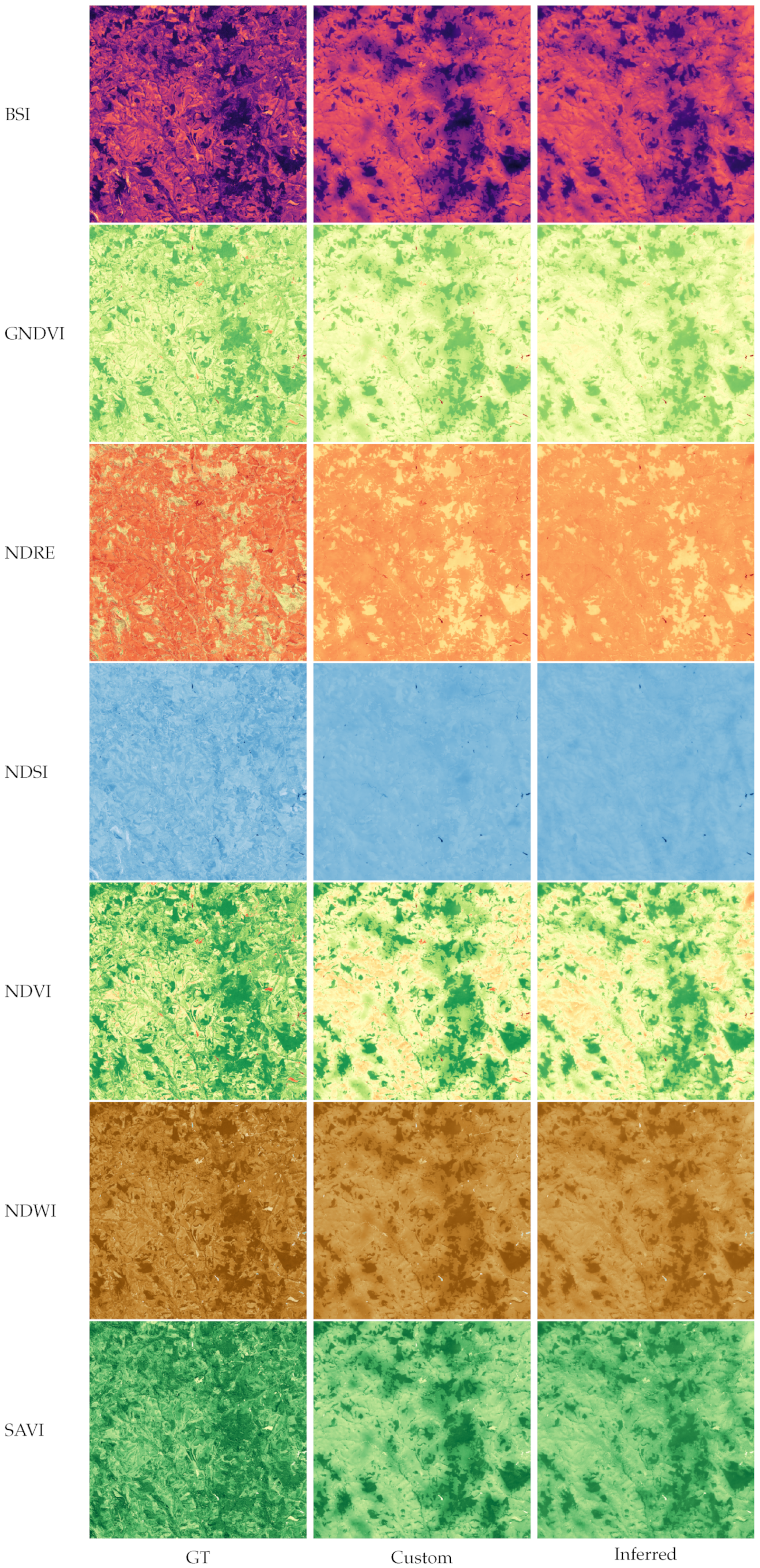
Figure 6 qualitatively confirms the quantitative evaluation reported in Table 3. For each index, the first column corresponds to the Sentinel-2 reference product, the second column to the direct SAR-to-index reconstruction (custom), and the third column to the indices derived from the reconstructed multispectral bands (inferred).

Overall, both approaches preserve the main spatial patterns and large-scale semantic structures of the target indices. The reconstructed products remain visually coherent with the corresponding ground truths, particularly for large homogeneous regions and high-contrast spatial structures. However, direct index-specific models generally recover finer spatial details more accurately than the multispectral reconstruction strategy.

The differences become more evident in vegetation-sensitive indices such as NDRE and NDVI. In these cases, the inferred-band approach occasionally misses localized high-response regions or produces smoother transitions compared to the custom models. This behavior is coherent with the previous spectral-band analysis, where NIR and red edge channels represented the most challenging bands to reconstruct.

At the same time, both approaches successfully preserve the dominant spatial responses of the indices. For example, strong-activation regions in NDSI are consistently reconstructed by both strategies, indicating that high-contrast semantic structures are effectively captured from SAR observations.

Despite the promising results, both approaches still exhibit limitations in reconstructing fine-scale spatial variability and sharp spectral transitions. Compared with the ground-truth products, the reconstructed indices tend to appear spatially smoother and occasionally amplify local contrast differences between bright and dark regions.

These observations suggest that SAR-based reconstruction is currently more reliable for large-scale spatial analysis and semantic interpretation than for precise radiometric estimation at fine spatial resolution. Nevertheless, the overall consistency between the reconstructed and reference indices demonstrates the feasibility of deriving meaningful vegetation and soil indicators directly from SAR observations.

6. Ablation Studies

6.1. Analysis of the Results per Class

In addition to the overall analysis of the reconstruction of the spectral information and of the indices in the entire scene, we also investigate the performance of these reconstructions, focusing on single classes of land cover from WorldCover. This analysis aims to study how well the conversions work on a specific type of land. The investigation is composed of two parts. The former is the analysis of the performance of the spectral reconstruction per band on specific land-cover classes. The latter investigates the relationship between the reconstruction of the indices and the specific land-cover area.

Both investigations consider MAE, PSNR, and SSIM, which are the three metrics used on the single bands and the single indices in the previous sections. For better readability of the results, we have combined the three metrics into a single score. The score is computed by normalizing each metric between its max and min values and then averaging their normalizations. In this score, the MAE is inverted to remain coherent with the increasing trend of PSNR and SSIM. The resulting scores are values between 0 and 1, where the higher the value the better. The first investigation considers Efficient-UNet, while the second one considers the inferred bands methodology.

In this analysis, the WorldCover classes are used as landscape-specific subsets of the test data. In particular, Cropland is used to analyze agricultural areas, Tree cover and Mangroves represent forested or woody vegetation conditions, while Bare/sparse vegetation is used as a proxy for arid or sparsely vegetated regions.

6.1.1. Spectral Bands per Class

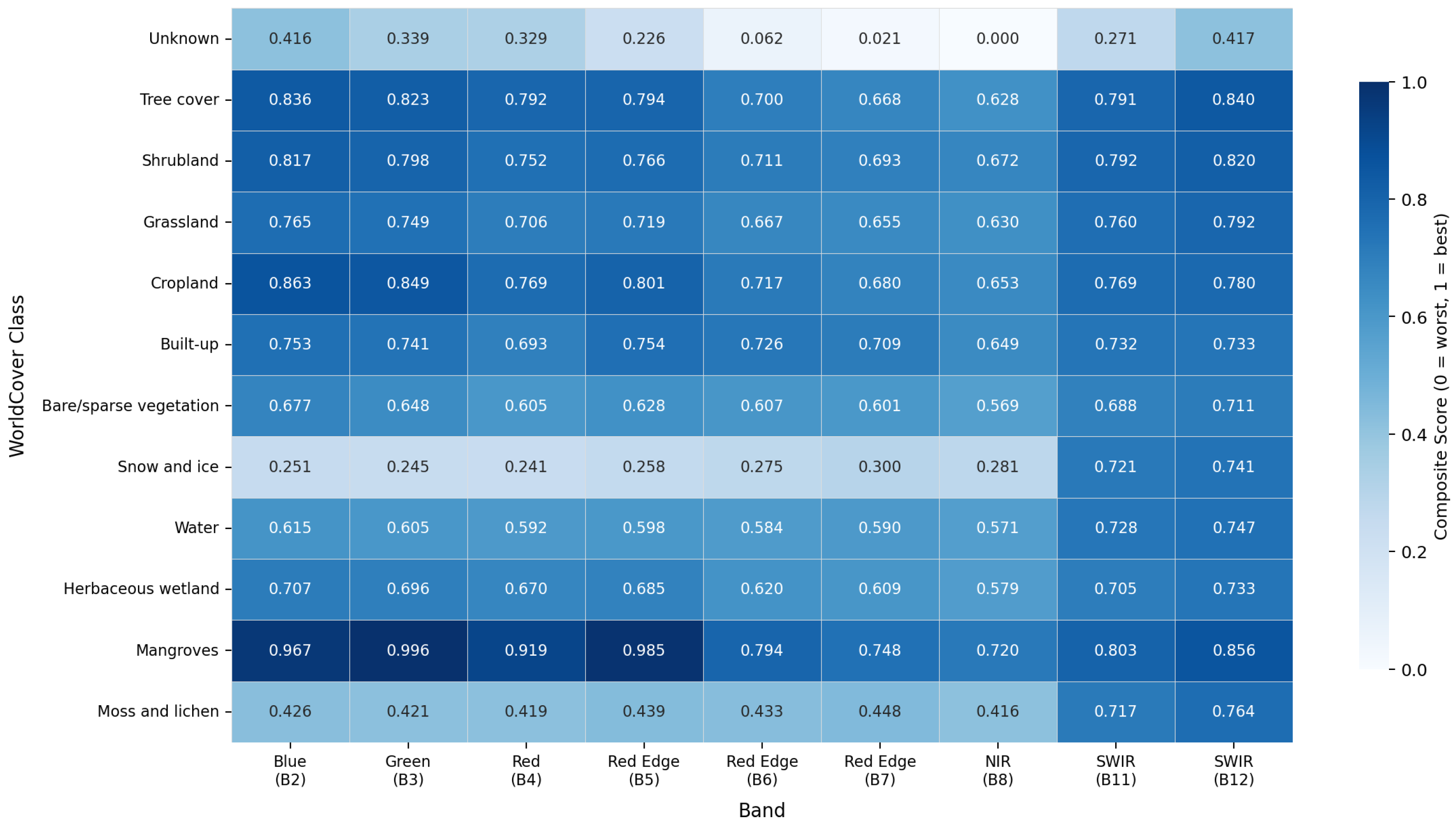
Figure 7 shows a heatmap which reports the scores achieved between the land-cover classes and the spectral bands reconstructed. It is important to note that scores are derived from min–max normalization, so values of 0 and 1 indicate the relatively worst- and best-performing cells in the matrix rather than indicating absolute failure or perfect reconstruction.

Focusing on the land-cover classes, it is immediately observable that most of the classes achieve a good score on all the bands. However, the model is not able to reconstruct the spectrum information of the Unknown, Snow and Ice, and Moss and lichen classes well, where it achieve the worse results overall. The Mangroves and vegetated classes, such as Tree cover, Shrubland, and Cropland, achieve the highest reconstruction scores, particularly in the visible and SWIR bands. This is consistent with the known sensitivity of SAR to vegetation structure, which correlates with the spectral response in these bands. Grassland and Herbaceous wetland show intermediate performance, reflecting a moderate SAR–spectral relationship. The same is observed for Built-up and Bare/sparse vegetation, which show moderate scores, suggesting that while SAR is sensitive to urban structures and bare soil roughness, the spectral diversity within these classes introduces uncertainty in the reconstruction, especially for the red edge and NIR bands. Snow and ice and Unknown show the lowest scores overall, particularly in the visible and red edge bands. For Snow and ice, this is expected: SAR backscatter over frozen surfaces is dominated by volume scattering and surface roughness effects that are poorly correlated with optical reflectance. The Unknown class, likely comprising mixed or unclassified pixels, shows inherently high spectral variability that SAR backscatter cannot reliably predict. Finally, the Water class also performs poorly in the visible and red edge range, though it partially recovers in the SWIR, where the near-zero reflectance of water creates a more predictable and consistent target.

Now, focusing instead on the spectral bands, we can confirm the conclusion of the previous sections. The reconstruction quality is highest in the visible bands (blue, green, and red) and in the SWIR bands, while it progressively degrades toward the NIR (b8) and the red edge bands (b6, b7). The general trend in the score, which degrades in those spectrum areas, is generally the same for all the classes, showing that there is no direct relationship between the reconstructed band and class.

Overall, these results suggest that SAR-to-multispectral reconstruction is most reliable for vegetated land cover and in the visible and SWIR spectral range, while it remains fundamentally limited for spectrally homogeneous or spectrally complex surfaces, where the SAR–optical relationship is weak or ambiguous. This has direct implications for index computation: indices relying on NIR and red edge bands, such as NDVI, NDRE, and SAVI, will carry higher reconstruction uncertainty than those exploiting SWIR or visible bands, such as NDSI and BSI.

6.1.2. Vegetation Indices per Class

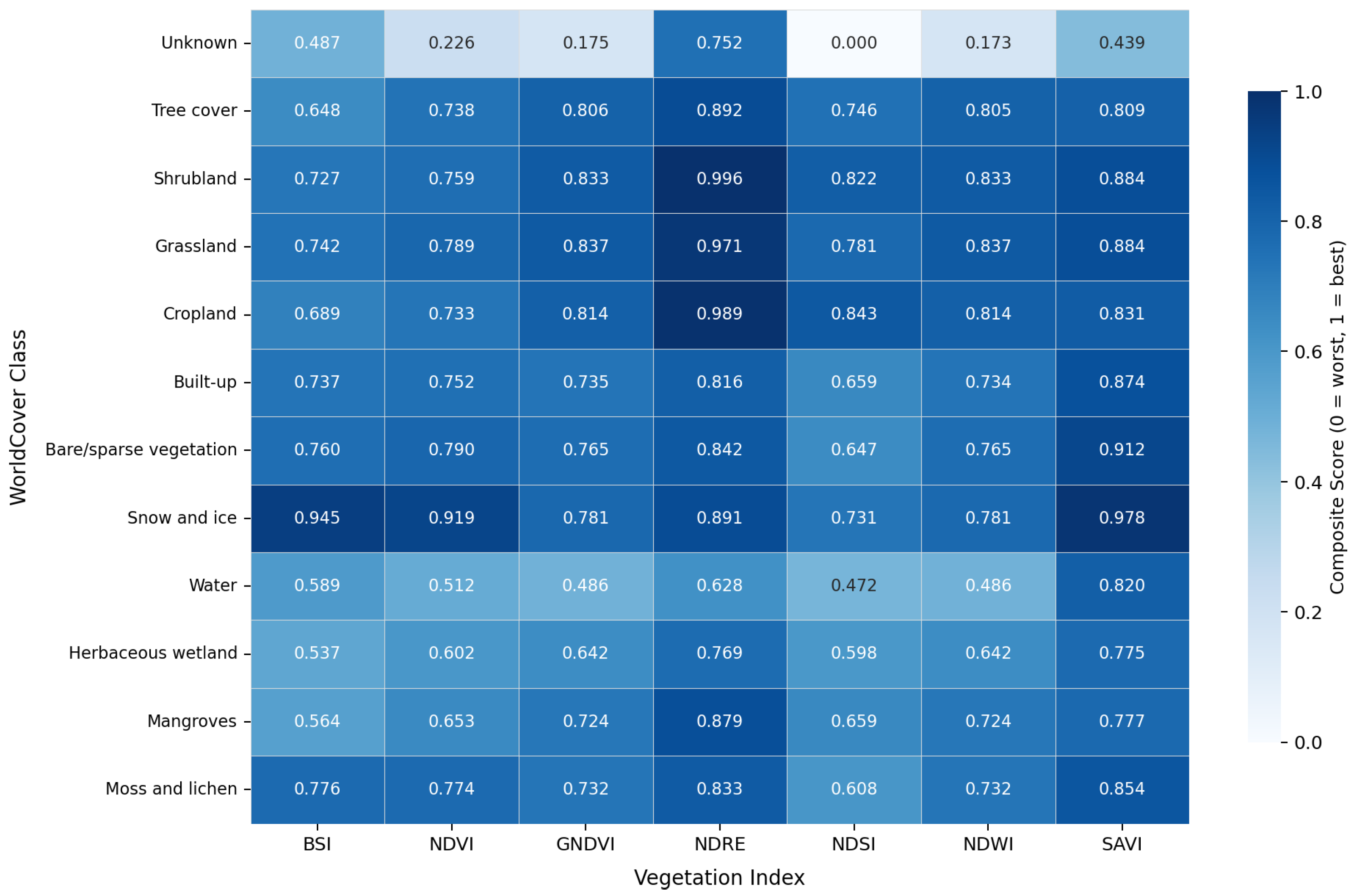
Figure 8 shows a heatmap that reports the relative scores achieved between the land-cover classes and the spectral bands reconstructed.

Focusing on the land-cover classes, Snow and ice, and vegetated classes such as Shrubland, Grassland, and Cropland achieve the highest overall reconstruction scores across indices. The strong performance for Snow and ice is partly attributable to the spectrally constrained and homogeneous nature of this class, which simplifies index reconstruction regardless of the underlying band-level accuracy. On the other hand, the vegetated classes Shrubland, Grassland, and Cropland achieve scores coherent with the established sensitivity of SAR backscatter to vegetation density and moisture conditions, and the better spectral reconstruction demonstrated on these land-cover areas (as discussed in Section 6.1.1).

On the other hand, Unknown and Water are the worst-performing classes. The Unknown class follows the same conclusion of the spectral reconstruction and is likely composed of mixed land-cover pixels for which the SAR and spectral relationship is not well defined. Instead, water bodies present near-zero reflectance in the NIR and red bands, making indices that exploit these bands (NDVI, NDRE, SAVI) unreliable even when the underlying band reconstruction is nominally accurate, reducing the overall performance of the class.

Now, considering the vegetation indices, we can confirm the already discussed behavior (see Section 5.2.1). It is noticeable that NDRE consistently achieves the highest mean score across all the classes, followed by SAVI. On the contrary, the other indices perform similarly over all the land-cover classes (not considering the Unknown class). Among them, NDSI, BSI, and NDVI perform comparatively poorly.

Discussing the relationship between the class and the vegetation indices, NDRE is the best-performing index for all vegetated classes (Tree cover, Shrubland, Grassland, Cropland, Mangroves), while SAVI dominates for non-vegetated or structurally complex classes (Built-up, Bare/sparse vegetation, Snow and ice, Water, Herbaceous wetland, Moss and lichen). Notably, GNDVI and NDWI produce near-identical scores across all classes. Considering that both rely on the NIR and green bands, differing only in index directionality, the moderate score achieved is due to the reconstruction errors of the NIR spectral band.

Generally, the results indicate that vegetation index reconstruction via inferred multispectral bands is most reliable for vegetated land cover and for vegetation indices, while multi-band indices, such as BSI and NDSI, and spectrally ambiguous classes, such as Unknown and Water, remain the most challenging targets.

6.2. Impact of SAR and WorldCover

To further analyze the usefulness of SAR in reconstructing soil indices and to investigate the performance similarities among different approaches, we investigate how well the indices can be estimated by removing or keeping the SAR as an input source. Specifically, using the custom model approach that gave us the best performance in terms of pure evaluation metrics, we compare the same approach in three different configurations for all the indices seen previously. These configurations take in input different sources of information and provide insight into the impact that the SAR data has on the final results. In particular, we test the multimodal approach described in the previous section, with SAR, DEM, and WorldCover, an approach that exploits only WorldCover, and an approach with only SAR as input.

Table 4. Result indices with Efficient-UNet using different configurations of features as an ablation study. Lower MAE and higher PSNR/SSIM indicate better reconstruction quality.

Metric	Index	SAR–DEM–WC	WC-Only	SAR-Only
MAE ↓	BSI	0.100 ± 0.057	0.123 ± 0.077	0.114 ± 0.060
	GNDVI	0.094 ± 0.050	0.126 ± 0.083	0.114 ± 0.059
	NDRE	0.042 ± 0.019	0.045 ± 0.022	0.045 ± 0.021
	NDSI	0.134 ± 0.131	0.195 ± 0.213	0.168 ± 0.159
	NDVI	0.102 ± 0.055	0.145 ± 0.096	0.121 ± 0.060
	NDWI	0.094 ± 0.050	0.126 ± 0.083	0.114 ± 0.060
	SAVI	0.066 ± 0.030	0.091 ± 0.055	0.077 ± 0.034
	Overall	0.090 ± 0.056	0.121 ± 0.090	0.108 ± 0.069
PSNR ↑	BSI	24.695 ± 4.529	23.496 ± 5.036	23.327 ± 4.013
	GNDVI	24.901 ± 4.226	23.414 ± 5.214	22.910 ± 4.374
	NDRE	31.421 ± 4.087	31.185 ± 4.330	30.466 ± 4.437
	NDSI	22.803 ± 6.146	21.199 ± 7.600	20.734 ± 6.285
	NDVI	24.416 ± 4.751	22.509 ± 5.945	22.727 ± 4.165
	NDWI	24.898 ± 4.225	23.422 ± 5.219	22.867 ± 4.433
	SAVI	28.193 ± 4.136	26.236 ± 5.273	26.689 ± 4.029
	Overall	25.904 ± 4.585	24.494 ± 5.517	24.246 ± 4.534
SSIM ↑	BSI	0.522 ± 0.272	0.452 ± 0.329	0.462 ± 0.266
	GNDVI	0.671 ± 0.190	0.620 ± 0.235	0.617 ± 0.231
	NDRE	0.631 ± 0.186	0.596 ± 0.223	0.599 ± 0.216
	NDSI	0.648 ± 0.205	0.579 ± 0.287	0.595 ± 0.229
	NDVI	0.627 ± 0.177	0.565 ± 0.218	0.562 ± 0.215
	NDWI	0.671 ± 0.190	0.620 ± 0.235	0.617 ± 0.231
	SAVI	0.679 ± 0.161	0.616 ± 0.209	0.626 ± 0.211
	Overall	0.636 ± 0.197	0.578 ± 0.247	0.583 ± 0.228

reports the performance achieved by the three configurations. The results show that the multimodal approach is the one that performs the best among the configurations. However, it is observable that, focusing on the single-modality configurations, the results achieved are overall competitive even without the multimodal approach. While this behavior might be expected in the SAR-only configuration, the results achieved by the WorldCover-only experiments are remarkable. In fact, when the single-modality approaches are compared, the performances are comparable. The SAR-only performance is slightly better when it comes to RMSE and SSIM, but the WorldCover-only configuration is unexpectedly able to outperform the SAR-only one in terms of PSNR. Performance-wise, this means that it is possible to achieve comparable reconstructions even by using only the semantic context of the scene, without having any kind of information about the structural characteristics of the area. This leads to two possible conclusions: either the reconstruction, independently of the tested input sources, is a too limited and too approximate estimation of the real indices; or the evaluation metrics typically used in this field are not accurate enough to describe the real value of our reconstruction.

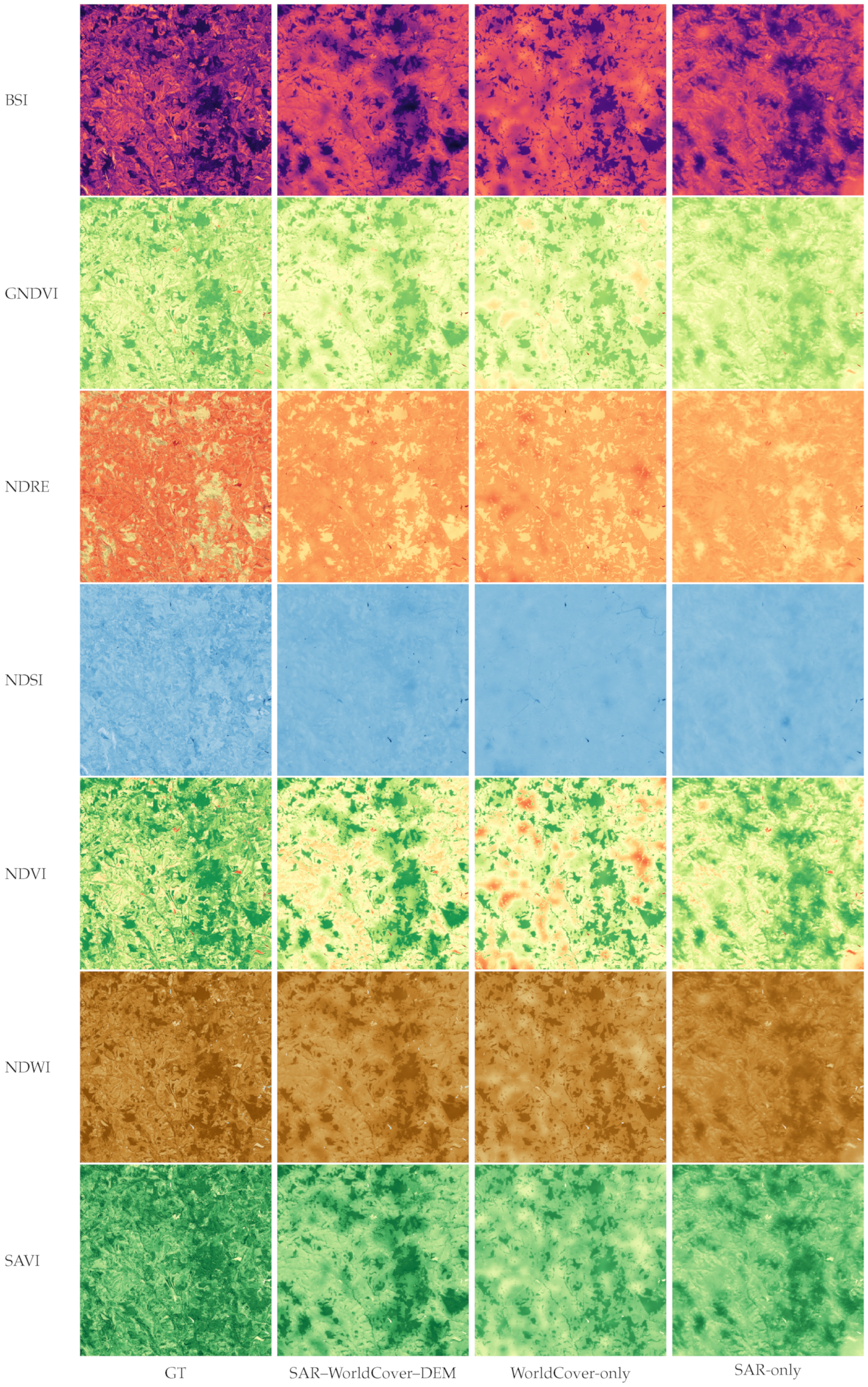
Figure 9 shows a visual comparison between the reconstructions achieved by the different configurations. It is clearly visible that all the configurations achieve different results. While the multimodal approach keeps all the limitations we have already described, it is closer to the ground truth. The other two configurations are less capable of reconstructing indices that resemble the real ones. Nonetheless, it is observable, in particular looking at NDVI, GNDVI, BSI, and SAVI, that the indices reconstructed using the WorldCover-only approach resemble the real indices the least. The results achieved by this configuration are completely lacking the fine details of the original indices, presenting a much more flattened reconstruction, probably derived from the nature of the input source, which does not capture this kind of information. In addition, the reconstructions show much greater contrast in comparison to the other configurations and the ground truths.

Considering the visual analysis, we can conclude two main points: (1) WorldCover, contrary to the suggestion from the metric performance, is not suitable to be used alone, but it represents auxiliary information; and (2) the evaluation metrics typically used for this task are not suitable and lead to wrong considerations about the real results of the model reconstructions.

These conclusions are reinforced by the statistical analysis of the configurations. The investigation shows that the multimodal configuration (SAR–WorldCover–DEM) is significantly superior to both single-modality baselines for most indices. In particular, regarding the comparison with the WorldCover-only and SAR-only approaches, for MAE, p < 0.003 and p < 0.013 are, respectively, obtained for five out of seven indices, while for SSIM, p < 0.03 is obtained for most indices except NDRE. This confirms that combining SAR, DEM, and WorldCover provides a statistically meaningful gain over any individual input source. However, the most critical finding concerns the comparison between the two single-modality configurations: WorldCover-only and SAR-only are not significantly different for any index across any metric. For MAE and for PSNR, all p-values are greater than 0.07, while for SSIM, the achieved p-values for all indices are greater than 0.50. This result provides statistical confirmation that, under the metrics and experimental conditions considered here, SAR backscatter does not carry demonstrably more predictive information than a static land-cover prior. While the visual results reveal qualitative differences that the metrics fail to capture, the quantitative equivalence of SAR-only and WorldCover-only reinforces the need for more discriminative evaluation protocols in SAR-based spectral reconstruction research.

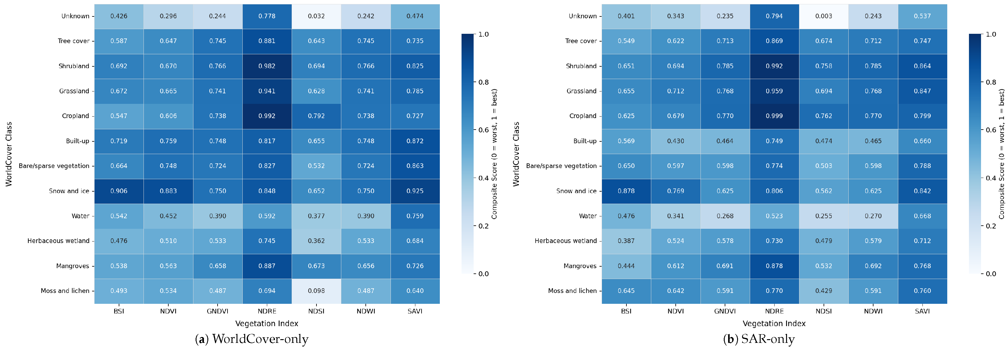
To complete the analysis, we investigate the impact of the two single-modality approaches on the land-cover classes. Figure 10 reports the heatmaps for the WorldCover-only (a) and SAR-only (b) approaches. The heatmaps were constructed in the same way as described in Section 6.1. In this investigation we wants to contextualize the performance of the multimodal approach by revealing how much each individual modality contributes and, at the same time, we want to highlight the complementary strengths and weaknesses of the two single-modality approaches across land-cover classes and vegetation indices. Both single-modality approaches reproduce similar structural patterns observed in the multimodal approach model. NDRE achieves the highest scores across all classes in both the WorldCover-only and SAR-only configurations. Similarly, SAVI ranks as the second-best index performance-wise in both configurations, in particular, for non-vegetated and structurally heterogeneous classes. NDSI, BSI, and NDVI remain in the same pattern, making the reconstruction results more difficult.

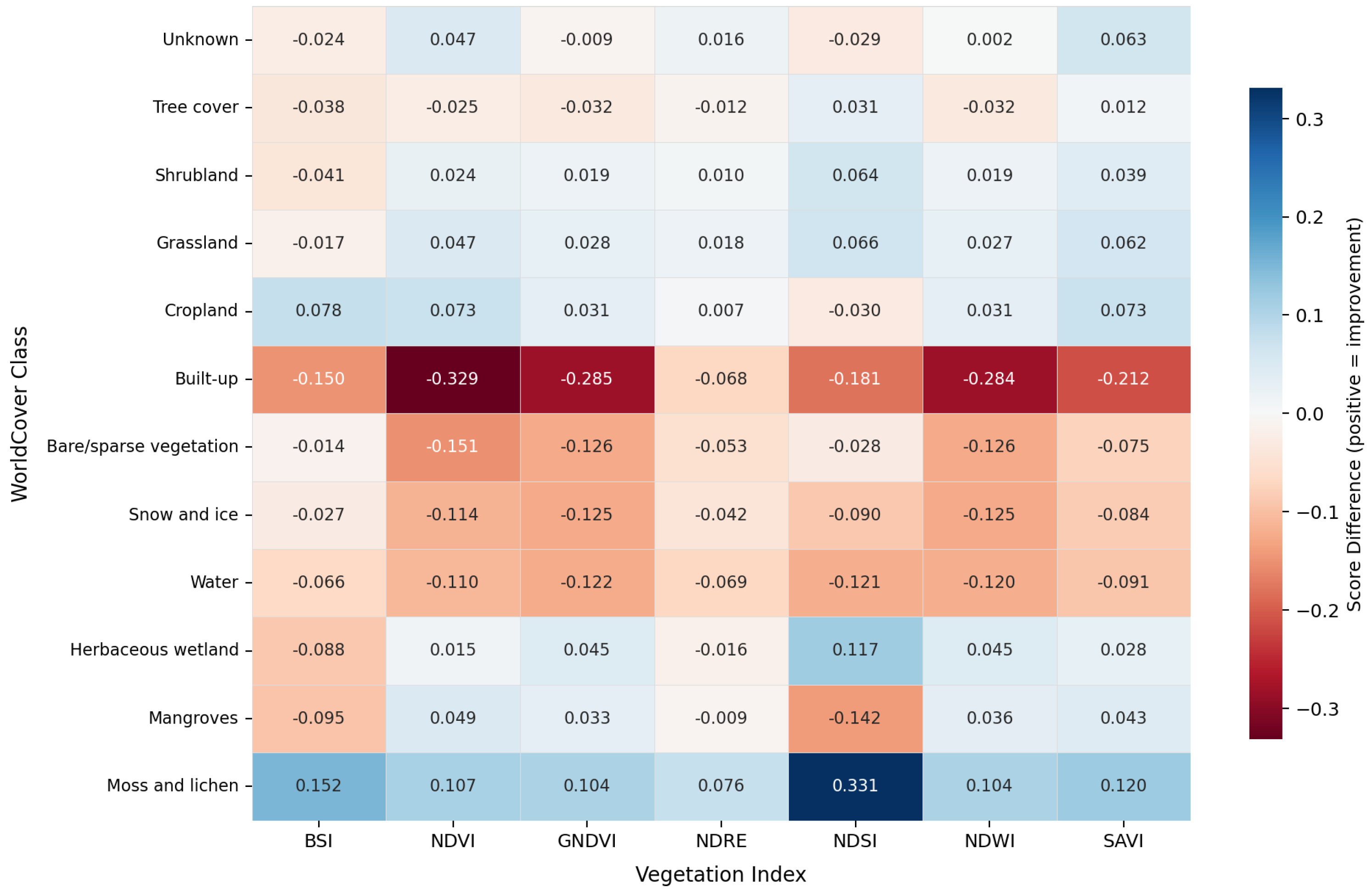
To better understand the difference between the two single-modality approaches, Figure 11 reports the difference between their two heatmaps. The red color indicates the cells where the WorldCover-only approach outperforms the SAR-only one, while the blue color indicates the opposite. Despite the structural similarity, the two configurations diverge substantially in specific class–index combinations. The most pronounced difference concerns the Built-up class, where WorldCover-only outperforms SAR-only across all indices. This is physically interpretable: SAR backscatter in urban environments is dominated by double-bounce and specular scattering from buildings and hard surfaces [45], which are structurally unrelated to the optical reflectance properties driving vegetation index values. WorldCover’s explicit categorical label for built-up areas provides a far more informative spectral prior for index reconstruction, explaining its substantial advantage. A similar, though less extreme, pattern is observed for Snow and ice and Bare/sparse vegetation, where WorldCover-only outperforms SAR-only for NDVI, GNDVI, and NDWI, as the categorical land-cover label constrains the model’s spectral prediction space more effectively than radar scattering mechanisms, which are largely decoupled from optical reflectance in these surface types. In contrast, SAR-only outperforms WorldCover-only for moisture-sensitive and dynamically varying classes. Herbaceous wetland shows consistent positive differences in favor of SAR for NDVI, GNDVI, NDSI, NDWI, and SAVI, reflecting the SAR’s sensitivity to surface and soil moisture dynamics, which a static land-cover label cannot capture. Along the same lines, the Moss and lichen class exhibits the largest positive differences in the entire heatmap, especially for NDSI.

Overall, the difference matrix reveals a clear modality-specificity principle: WorldCover categorical priors are more effective for spectrally constrained, structurally complex, or optically homogeneous surfaces (Built-up, Snow and ice, Water), where radar backscatter carries little information relevant to optical index computation, while SAR is more effective for dynamic, moisture-sensitive, or structurally variable vegetation types (Wetlands, Cropland, Mangroves, Moss and lichen), where static land-cover labels fail to capture the within-class spectral variability that SAR can partially resolve. These results explain why combining the two modalities improves the overall quality of the reconstruction, highlighting the complementary nature of the two modalities.

7. Conclusions

Thanks to SAR’s robustness to different weather conditions, estimating soil indices from SAR data helps to analyze soil characteristics and can replace the extraction of indices from multispectral optical data, which are particularly weather-sensitive. In this article, we compare two approaches for converting SAR to indices, investigating their limitations and, more generally, studying the limitations of studies on this conversion.

The first approach converts SAR directly to a specific index. Although this approach is the most widely studied and used in SOTA [27], it lacks flexibility. This is because a specific model needs to be trained and personalized for each desired index, which makes it difficult and time-consuming to extract different soil characteristics in a specific area. For this reason, the second approach we propose and analyze converts SAR to multispectral data rather than a specific index. The multispectral bands derived from SAR can then be used to extract additional indices as required, without the need for specific models. To compare the two approaches, we first trained a model to extract all the necessary spectral information, testing different SOTA techniques and evaluating the most effective one. Secondly, we compared the indices extracted from the inferred spectral bands with those extracted by training index-specific models.

The results on the SEN12TP dataset show that, although the index-specific models slightly outperform the multispectral-based approach in terms of numerical metrics, the performance achieved by the two strategies is comparable both quantitatively and visually. This supports the initial motivation of the proposed framework: in practical scenarios, reconstructing multispectral information first can provide a more flexible solution, since multiple indices can be derived from the same predicted product without training a dedicated model for each target index.

These findings are consistent with the broader SAR-to-optical and SAR-based vegetation monitoring literature. Previous SAR-to-optical translation studies have often focused on visually plausible RGB reconstruction, RGB+NIR synthesis, or on a limited subset of optical bands [6]. More recent studies have started to address SAR-to-multispectral reconstruction more explicitly, for instance, through architectures designed to generate Sentinel-2-like multispectral products from SAR observations [7]. Compared with these studies, the present work does not focus only on the reconstruction of an optical-like image, but evaluates multispectral reconstruction as an intermediate representation for deriving multiple downstream vegetation and soil indices within a single framework.

This distinction is also relevant with respect to direct SAR-to-index approaches, where a separate model is typically required for each target index. While direct models can provide slightly better performance for the specific index on which they are trained, they are less flexible when several indicators are required simultaneously. Conversely, the SAR-to-multispectral strategy enables the computation of different indices from the same reconstructed spectral bands. Therefore, the significance of the proposed framework lies not only in its reconstruction accuracy, but also in its operational flexibility and reduced need for multiple index-specific training procedures.

However, the results also confirm that SAR-based reconstruction remains intrinsically limited. In the multispectral reconstruction setting, the tested methods are generally able to recover the large-scale spatial structure of the scene, but they do not fully preserve the fine spectral details of the original Sentinel-2 bands. These missing details are then propagated to the derived indices. A similar limitation is observed for the direct SAR-to-index models: even when a model is trained specifically for a given index, part of the fine spatial and spectral variability of the optical reference is still lost. For these reasons, regardless of the adopted strategy, the estimated indices should be considered approximate reconstructions rather than exact replacements of the original optical products.

To further analyze this limitation, we performed an ablation study to assess the actual contribution of the different input modalities. We considered the full multimodal configuration, including SAR, DEM, and WorldCover, as well as reduced configurations based on individual or partial inputs. The results confirm the limitations of SAR-based reconstruction, but also suggest that conventional pixel-wise metrics alone may not fully capture the semantic and structural quality of the reconstructed products. Indeed, although some configurations achieve comparable numerical performance, their visual outputs show clear differences. This indicates that future evaluations should include metrics that better reflect spatial structure, semantic consistency, and downstream usability, rather than relying only on pixel-wise similarity.

The relationship between SAR backscatter and optical vegetation indices can also be interpreted in light of radar-based vegetation descriptors such as the Radar Vegetation Index (RVI). Previous studies have shown that the RVI and dual-polarimetric RVI formulations derived from Sentinel-1 data are sensitive to crop growth dynamics and to biophysical vegetation variables [46,47]. However, this relationship is intrinsically indirect. Radar vegetation indices are mainly governed by microwave scattering mechanisms related to canopy structure, dielectric properties, surface roughness, and moisture conditions, whereas optical indices such as NDVI, GNDVI, NDRE, and SAVI are derived from visible, red edge, and near-infrared reflectance responses associated with greenness, chlorophyll absorption, canopy vigor, and soil-background effects. Similarly, NDWI is influenced by water-related optical contrast and may therefore exhibit a more context-dependent relationship with radar backscatter. Recent analyses of the SAR–NDVI relationship also show that this link varies with crop type, phenological stage, radar frequency, polarization, and acquisition geometry, and that RVI is not necessarily more correlated with NDVI than individual SAR polarization channels [48].

This physical interpretation supports the main conclusion of the study: SAR-based models can recover part of the dominant spatial organization of optical vegetation indices, but the reconstructed indices should be regarded as SAR-informed optical proxies rather than physically equivalent substitutes for optical measurements. In this perspective, SAR represents a valuable complementary modality for Earth observation applications, especially under cloudy or illumination-limited conditions, but not a complete substitute for multispectral optical data. Future work should therefore investigate alternative evaluation strategies for vegetation index reconstruction, including metrics that better capture semantic and structural consistency beyond pixel-wise similarity, as well as hybrid approaches that explicitly combine radar and optical information when available. In addition, the reconstruction of spectral information should focus, in particular, on improving the reconstruction of NIR and red edge bands, which are fundamental for some of the most used vegetation indices and therefore need the reconstruction to be as close as possible to the real spectral values.

References

1. Giovos, R.; Tassopoulos, D.; Kalivas, D.; Lougkos, N.; Priovolou, A. Remote sensing vegetation indices in viticulture: A critical review. Agriculture 2021, 11, 457. [Google Scholar] [CrossRef]
2. Montero, D.; Aybar, C.; Mahecha, M.D.; Martinuzzi, F.; Söchting, M.; Wieneke, S. A standardized catalogue of spectral indices to advance the use of remote sensing in Earth system research. Sci. Data 2023, 10, 197. [Google Scholar] [CrossRef] [PubMed]
3. Xiong, Q.; Li, G.; Yao, X.; Zhang, X. SAR-to-optical image translation and cloud removal based on conditional generative adversarial networks: Literature survey, taxonomy, evaluation indicators, limits and future directions. Remote Sens. 2023, 15, 1137. [Google Scholar] [CrossRef]
4. Sommervold, O.; Gazzea, M.; Arghandeh, R. A survey on SAR and optical satellite image registration. Remote Sens. 2023, 15, 850. [Google Scholar] [CrossRef]
5. Schmitt, M.; Hughes, L.H.; Zhu, X.X. The SEN1-2 Dataset for Deep Learning in SAR-Optical Data Fusion. ISPRS Ann. Photogramm. Remote Sens. Spat. Inf. Sci. 2018, IV-1, 141–146. [Google Scholar] [CrossRef]
6. Zhang, Q.; Liu, X.; Liu, M.; Zou, X.; Zhu, L.; Ruan, X. Comparative analysis of edge information and polarization on sar-to-optical translation based on conditional generative adversarial networks. Remote Sens. 2021, 13, 128. [Google Scholar] [CrossRef]
7. Liu, Y.; Han, Q.; Yang, H.; Hu, H. High-Resolution SAR-to-Multispectral Image Translation Based on S2MS-GAN. Remote Sens. 2024, 16, 4045. [Google Scholar] [CrossRef]
8. Wei, J.; Zhou, H.; Ke, P.; Ma, Y.; Tang, R. Sequential SAR-to-Optical Image Translation. Remote Sens. 2025, 17, 2287. [Google Scholar] [CrossRef]
9. Wang, L.; Xu, X.; Yu, Y.; Yang, R.; Gui, R.; Xu, Z.; Pu, F. SAR-to-optical image translation using supervised cycle-consistent adversarial networks. IEEE Access 2019, 7, 129136–129149. [Google Scholar] [CrossRef]
10. Enomoto, K.; Sakurada, K.; Wang, W.; Kawaguchi, N.; Matsuoka, M.; Nakamura, R. Image translation between SAR and optical imagery with generative adversarial nets. In Proceedings of the 2018 IEEE International Geoscience and Remote Sensing Symposium (IGARSS), Valencia, Spain, 22–27 July 2018; IEEE: New York, NY, USA, 2018; pp. 1752–1755. [Google Scholar]
11. Fu, S.; Xu, F.; Jin, Y.Q. Reciprocal translation between SAR and optical remote sensing images with cascaded-residual adversarial networks. Sci. China Inf. Sci. 2021, 64, 122301. [Google Scholar] [CrossRef]
12. Tan, D.; Liu, Y.; Li, G.; Yao, L.; Sun, S.; He, Y. Serial GANs: A feature-preserving heterogeneous remote sensing image transformation model. Remote Sens. 2021, 13, 3968. [Google Scholar] [CrossRef]
13. Guo, J.; He, C.; Zhang, M.; Li, Y.; Gao, X.; Song, B. Edge-preserving convolutional generative adversarial networks for SAR-to-optical image translation. Remote Sens. 2021, 13, 3575. [Google Scholar] [CrossRef]
14. Yang, X.; Zhao, J.; Wei, Z.; Wang, N.; Gao, X. SAR-to-optical image translation based on improved CGAN. Pattern Recognit. 2022, 121, 108208. [Google Scholar] [CrossRef]
15. Li, H.; Gu, C.; Wu, D.; Cheng, G.; Guo, L.; Liu, H. Multiscale generative adversarial network based on wavelet feature learning for SAR-to-optical image translation. IEEE Trans. Geosci. Remote Sens. 2022, 60, 5236115. [Google Scholar] [CrossRef]
16. Wei, J.; Zou, H.; Sun, L.; Cao, X.; He, S.; Liu, S.; Zhang, Y. CFRWD-GAN for SAR-to-optical image translation. Remote Sens. 2023, 15, 2547. [Google Scholar] [CrossRef]
17. Wang, Z.; Ma, Y.; Zhang, Y. Hybrid cGAN: Coupling global and local features for SAR-to-optical image translation. IEEE Trans. Geosci. Remote Sens. 2022, 60, 5236016. [Google Scholar] [CrossRef]
18. Shi, H.; Cui, Z.; Chen, L.; He, J.; Yang, J. A brain-inspired approach for SAR-to-optical image translation based on diffusion models. Front. Neurosci. 2024, 18, 1352841. [Google Scholar] [CrossRef] [PubMed]
19. Seo, M.; Jung, J.; Choi, D.G. Improved Flood Insights: Diffusion-Based SAR-to-EO Image Translation. Remote Sens. 2025, 17, 2260. [Google Scholar] [CrossRef]
20. Bai, X.; Pu, X.; Xu, F. Conditional Diffusion for SAR to Optical Image Translation. IEEE Geosci. Remote Sens. Lett. 2024, 21, 4000605. [Google Scholar] [CrossRef]
21. Zhang, M.; Zhang, P.; Zhang, Y.; Yang, M.; Li, X.; Dong, X.; Yang, L. SAR-to-optical image translation via an interpretable network. Remote Sens. 2024, 16, 242. [Google Scholar] [CrossRef]
22. Zhang, M.; He, C.; Zhang, J.; Yang, Y.; Peng, X.; Guo, J. SAR-to-Optical Image Translation via Neural Partial Differential Equations. In Proceedings of the International Joint Conference on Artificial Intelligence (IJCAI), Vienna, Austria, 23–29 July 2022; pp. 1644–1650. [Google Scholar]
23. Charoenthammakim, D.; Ganokratanaa, T.; Ketcham, M.; Varnakovida, P.; Worasucheep, C.; Wattanapornprom, W. ReflectanceGAN: Geospatial SAR-to-MSI Translation for Cloud-Agnostic Sentinel-2 Analytics. In Proceedings of the 2025 20th International Joint Symposium on Artificial Intelligence and Natural Language Processing (iSAI-NLP), Phuket, Thailand, 12–14 November 2025; IEEE: New York, NY, USA, 2025; pp. 1–6. [Google Scholar]
24. Schmitt, M.; Hughes, L.H.; Qiu, C.; Zhu, X.X. SEN12MS—A Curated Dataset of Georeferenced Multi-Spectral Sentinel-1/2 Imagery for Deep Learning and Data Fusion. ISPRS Ann. Photogramm. Remote Sens. Spat. Inf. Sci. 2019, IV-2/W7, 153–160. [Google Scholar] [CrossRef]
25. Ebel, P.; Xu, Y.; Schmitt, M.; Zhu, X.X. SEN12MS-CR-TS: A Remote Sensing Data Set for Multi-Modal and Multi-Temporal Cloud Removal. arXiv 2022, arXiv:2201.09613. [Google Scholar] [CrossRef]
26. Roßberg, T.; Schmitt, M. SEN12TP—Sentinel-1 and -2 Images, Timely Paired; Zenodo: Geneva, Switzerland, 2023. Available online: https://zenodo.org/records/7342060 (accessed on 13 July 2026).
27. Roßberg, T.; Schmitt, M. A Globally Applicable Method for NDVI Estimation from Sentinel-1 SAR Backscatter Using a Deep Neural Network and the SEN12TP Dataset. PFG—J. Photogramm. Remote Sens. Geoinf. Sci. 2023, 91, 171–187. [Google Scholar] [CrossRef]
28. Bonafilia, D.; Tellman, B.; Anderson, G.; Huyck, J.I.B. Sen1Floods11: A Georeferenced Dataset to Train and Test Deep Learning Flood Algorithms for Sentinel-1. In Proceedings of the IEEE/CVF Conference on Computer Vision and Pattern Recognition Workshops (CVPRW), Seattle, WA, USA, 13–19 June 2020; pp. 210–219. [Google Scholar]
29. Rambour, C.; Ghamisi, P.; Audebert, N.; Lefèvre, M.; Velasco-Forero, S.; Boulch, A.; Sebastianelli, M.; Molin, M.D.; Ménage, R.; Dedieu, M.; et al. Flood Detection in Time Series of Optical and SAR Images. Int. Arch. Photogramm. Remote Sens. Spat. Inf. Sci. 2020, XLIII-B2, 1343–1350. [Google Scholar] [CrossRef]
30. European Space Agency. ESA WorldCover Data Access and Validation (2020–2021). Project Portal. 2025. Available online: https://esa-worldcover.org/en (accessed on 13 July 2026).
31. ESA WorldCover Consortium. WorldCover 10 m 2021 v200. Google Earth Engine Data Catalog, 2021. Available online: https://developers.google.com/earth-engine/datasets/catalog/ESA_WorldCover_v200 (accessed on 13 July 2026).
32. Zanaga, D.; Van De Kerchove, R.; Daems, D.; De Keersmaecker, W.; Brockmann, C.; Kirches, G.; Wevers, J.; Cartus, O.; Santoro, M.; Fritz, S.; et al. ESA WorldCover 10 m 2021 v200. 2022. Available online: https://zenodo.org/records/7254221 (accessed on 13 July 2026).
33. Small, D. Flattening gamma: Radiometric terrain correction for SAR imagery. IEEE Trans. Geosci. Remote Sens. 2011, 49, 3081–3093. [Google Scholar] [CrossRef]
34. Vollrath, A.; Mullissa, A.; Reiche, J. Angular-based radiometric slope correction for Sentinel-1 on google earth engine. Remote Sens. 2020, 12, 1867. [Google Scholar] [CrossRef]
35. Tan, M.; Le, Q.V. EfficientNetV2: Smaller Models and Faster Training. arXiv 2021, arXiv:2104.00298. [Google Scholar] [CrossRef]
36. Isola, P.; Zhu, J.Y.; Zhou, T.; Efros, A.A. Image-to-image translation with conditional adversarial networks. In Proceedings of the IEEE Conference on Computer Vision and Pattern Recognition, Honolulu, HI, USA, 21–26 July 2017; IEEE: New York, NY, USA, 2017; pp. 1125–1134. [Google Scholar]
37. Lipman, Y.; Chen, R.T.; Ben-Hamu, H.; Nickel, M.; Le, M. Flow matching for generative modeling. arXiv 2022, arXiv:2210.02747. [Google Scholar]
38. Tong, A.; Fatras, K.; Malkin, N.; Huguet, G.; Zhang, Y.; Rector-Brooks, J.; Wolf, G.; Bengio, Y. Improving and generalizing flow-based generative models with minibatch optimal transport. arXiv 2023, arXiv:2302.00482. [Google Scholar]
39. Mardan, M.; Ahmadi, S. Soil moisture retrieval over agricultural fields through integration of synthetic aperture radar and optical images. GISci. Remote Sens. 2021, 58, 1276–1299. [Google Scholar] [CrossRef]
40. Cagnina, C.; Marino, A.; Silva-Perez, C.; Ruiz-Ramos, J.; Suarez, J. Assessment of the Impact of Surface Water Content for Temperate Forests in SAR Data at C-Band. Remote Sens. 2023, 15, 5723. [Google Scholar] [CrossRef]
41. Li, X.; Zhu, B.; Li, S.; Liu, L.; Song, K.; Liu, J. A Comprehensive Review of Crop Chlorophyll Mapping Using Remote Sensing Approaches: Achievements, Limitations, and Future Perspectives. Sensors 2025, 25, 2345. [Google Scholar] [CrossRef] [PubMed]
42. Zhang, H.; Li, J.; Liu, Q.; Lin, S.; Huete, A.; Liu, L.; Croft, H.; Clevers, J.G.; Zeng, Y.; Wang, X.; et al. A novel red-edge spectral index for retrieving the leaf chlorophyll content. Methods Ecol. Evol. 2022, 13, 2771–2787. [Google Scholar] [CrossRef]
43. Ceccato, P.; Flasse, S.; Tarantola, S.; Jacquemoud, S.; Grégoire, J.M. Detecting vegetation leaf water content using reflectance in the optical domain. Remote Sens. Environ. 2001, 77, 22–33. [Google Scholar] [CrossRef]
44. Slaton, M.R.; Raymond Hunt, E., Jr.; Smith, W.K. Estimating near-infrared leaf reflectance from leaf structural characteristics. Am. J. Bot. 2001, 88, 278–284. [Google Scholar] [CrossRef] [PubMed]
45. Chauhan, S.; Srivastava, H.S. Comparative evaluation of the sensitivity of multi-polarised SAR and optical data for various land cover classes. Int. J. Adv. Remote Sens. Gis Geogr. 2016, 4, 1–14. [Google Scholar] [CrossRef]
46. Mandal, D.; Kumar, V.; Ratha, D.; Dey, S.; Bhattacharya, A.; Lopez-Sanchez, J.M.; McNairn, H.; Rao, Y.S. Dual polarimetric radar vegetation index for crop growth monitoring using Sentinel-1 SAR data. Remote Sens. Environ. 2020, 247, 111954. [Google Scholar] [CrossRef]
47. Hu, X.; Li, L.; Huang, J.; Zeng, Y.; Zhang, S.; Su, Y.; Hong, Y.; Hong, Z. Radar vegetation indices for monitoring surface vegetation: Developments, challenges, and trends. Sci. Total Environ. 2024, 945, 173974. [Google Scholar] [CrossRef] [PubMed]
48. Roßberg, T.; Schmitt, M. Comparing the relationship between NDVI and SAR backscatter across different frequency bands in agricultural areas. Remote Sens. Environ. 2025, 319, 114612. [Google Scholar] [CrossRef]
Figure 1. SEN12TP global distribution of the scenes collected in the dataset, divided into train and test, with the original split [27]. Blue areas represent train samples, while red areas represent test samples.
Remotesensing 18 02400 g001
Figure 2. SEN12TP distribution of the scenes per month and seasonality.
Remotesensing 18 02400 g002
Figure 3. WorldCover distribution in terms of number of percentage of pixels belonging to land-cover classes. The total number of pixels corresponds to 9,285,584,472.
Remotesensing 18 02400 g003
Figure 4. Schematic representation of the proposed workflow adopted in this study. Sentinel-1 backscatter coefficients, ESA WorldCover labels, and elevation data are first spatially aligned and concatenated into a multimodal input tensor. The resulting scenes are partitioned into patches and processed by the SAR-to-optical network to reconstruct Sentinel-2 spectral bands. Predicted patches are then aggregated to obtain the full-scene multispectral product. During evaluation, spectral indices are computed both from the original Sentinel-2 observations and from the reconstructed multispectral bands. The resulting index maps are finally compared through quantitative metrics, namely, mean absolute error (MAE), structural similarity index measure (SSIM), and peak signal-to-noise ratio (PSNR).
Remotesensing 18 02400 g004
Figure 5. Qualitative comparison between Sentinel-2 reference bands and the corresponding reconstructions generated by the Efficient-UNet model. For each example, the left image corresponds to the ground truth, the center image to the reconstructed band, and the right image to the absolute reconstruction error. All visualizations are displayed using false-color representations.
Remotesensing 18 02400 g005
Figure 6. Qualitative comparison between the reference spectral indices (GT), the direct SAR-to-index reconstruction approach (custom), and the indices derived from reconstructed multispectral bands (inferred).
Remotesensing 18 02400 g006
Figure 7. Relative score achieved by averaging the normalized metrics MAE (inverted), PSNR, and SSIM, achieved on the reconstruction of single spectral bands per class. The higher the score, the better.
Remotesensing 18 02400 g007
Figure 8. Relative score achieved by averaging the normalized metrics MAE (inverted), PSNR, and SSIM, achieved on the reconstruction of vegetation indices per land-cover class using the inferred band methodology. The higher the score, the better.
Remotesensing 18 02400 g008
Figure 9. Qualitative comparison between the reference spectral indices (GT), the SAR–WorldCover–DEM, WorldCover-only, and SAR-only index reconstructions with custom models.
Remotesensing 18 02400 g009
Figure 10. Relative score achieved by averaging the normalized metrics MAE (inverted), PSNR, and SSIM achieved on the reconstruction of vegetation indices per land-cover class using custom models with the WorldCover-only (a) and SAR-only (b) approaches. The higher the score, the better.
Remotesensing 18 02400 g010
Figure 11. Difference between the score achieved by the reconstruction of vegetation indices per class using custom models with the SAR-only and WorldCover-only approaches. The red color indicates the cells where the WorldCover-only approach outperforms the SAR-only one, while the blue color shows the opposite.
Remotesensing 18 02400 g011