Article

Long-Term Vegetation Dynamics Across Distance Buffers Along the Gonghe–Yushu Expressway Corridor on the Qinghai–Xizang Plateau


1
School of Civil Engineering, Northwest Minzu University, Lanzhou 730030, China
2
State Key Laboratory of Cryospheric Science and Frozen Soil Engineering, Northwest Institute of Eco-Environment and Resources, Chinese Academy of Sciences, Lanzhou 730030, China
*
Author to whom correspondence should be addressed.
Remote Sens. 2026, 18(14), 2354; https://doi.org/10.3390/rs18142354
Submission received: 28 May 2026 / Revised: 3 July 2026 / Accepted: 10 July 2026 / Published: 14 July 2026
(This article belongs to the Section Ecological Remote Sensing)

Highlights

What are the main findings?
  • Landsat observations from 2000 to 2025 reveal widespread vegetation greening along the Gonghe-Yushu Expressway corridor, with no significant decreasing NDVI trends detected at 30 m resolution.
  • The greening trend was established before expressway construction and remained broadly parallel across distance buffers, while NDVI was more strongly associated with warming than precipitation.
What are the implications of the main findings?
  • Multi-decadal remote sensing and buffer-zone analysis can help distinguish regional climate-related greening from road-associated vegetation signals in alpine infrastructure corridors.
  • Potential fine-scale roadside impacts may be masked at Landsat and kilometer-buffer scales, highlighting the need for targeted high-resolution monitoring near transport infrastructure.

Abstract

Highway construction in alpine environments of the Qinghai-Xizang Plateau (QXP) raises concerns about vegetation degradation and ecosystem disruption. However, the long-term ecological dynamics along newer expressway corridors on the QXP remain insufficiently understood. This study investigated vegetation dynamics and land use/land cover (LULC) changes along the Gonghe-Yushu Expressway (G0613, 634 km) corridor from 2000 to 2025, spanning the pre-construction, construction (2011–2017), and post-construction operational periods. Using 25 years of Landsat 5/7/8/9 imagery, we analyzed NDVI trends with Sen’s slope and Mann-Kendall tests, classified LULC into four classes (Grassland, Bare land, Water body, Built-up) using Random Forest, and examined NDVI—climate relationships using TerraClimate data. The results revealed a widespread and significant greening trend, with 77.3% of pixels showing significant NDVI increases (+0.0026/year) and no significant decreasing trends. The greening was established before highway construction and continued uniformly through all periods, with no detectable distance-dependent gradient across buffer zones (0–1, 1–2, 2–5, 5–10 km). LULC transitions were limited, with Bare land and Grassland as the dominant classes in the buffer corridor. NDVI was strongly correlated with temperature (ρ = 0.748, p < 0.001), which increased by +0.068 °C/year over the study period, while precipitation showed no significant trend. These findings indicate that vegetation greening co-varied with regional warming, while no persistent distance-dependent highway-associated NDVI signal was detected at the analyzed scale. Localized roadside impacts may remain unresolved at 30 m resolution, and the long-term implications of continued warming warrant continued monitoring.

1. Introduction

The Qinghai-Xizang Plateau (QXP), often referred to as the “Third Pole” of the Earth, is the highest and most extensive plateau on the planet, covering approximately 2.5 million km2 with an average elevation exceeding 4000 m [1]. The QXP harbors unique and fragile alpine ecosystems, including alpine meadows, alpine steppes, wetlands, and permafrost landscapes, which provide critical ecosystem services such as carbon sequestration, water regulation, and biodiversity conservation [2]. However, these ecosystems are highly sensitive to climate change and human disturbance, and have experienced significant degradation in recent decades [3].
Transportation infrastructure construction has been one of the major drivers of ecological change on the QXP. Extensive road and railway networks have been built across the plateau to support economic development and regional connectivity [4]. The Qinghai-Tibet Railway and Qinghai-Tibet Highway have received considerable scientific attention regarding their ecological impacts, including vegetation responses and broader biophysical effects along transport corridors [5,6]. Road construction and operation can alter vegetation cover, disrupt wildlife corridors, modify surface hydrology, and accelerate permafrost degradation, particularly within the immediate roadside corridor [7,8].
The Gonghe-Yushu Expressway (G0613) is a 634 km highway traversing the northeastern QXP from Gonghe County to Yushu City (Maduo County), with elevations ranging from approximately 2900 to 4500 m. Construction began in 2011, with the first phase completed in December 2014 and the full expressway opening to traffic on 1 August 2017. The highway passes through several ecologically sensitive zones, including alpine meadows, wetlands, and permafrost regions, connecting the Qinghai Lake Basin to the upper reaches of the Yangtze and Mekong Rivers. Despite the ecological significance of this corridor, systematic monitoring of vegetation dynamics and land use changes along the Gonghe-Yushu Expressway remains limited. Most existing studies on QXP road ecology have focused on the Qinghai-Tibet Railway or Highway, while the ecological impacts of newer expressways in the region have received relatively little attention.
Satellite remote sensing provides an effective and cost-efficient approach for monitoring long-term ecological changes across large and inaccessible areas [9]. The Normalized Difference Vegetation Index (NDVI), derived from Landsat or MODIS imagery, has been widely used as a proxy for vegetation cover, productivity, and ecosystem health on the QXP [10,11,12]. Recent QXP vegetation mapping studies have further demonstrated the value of long time-series remote sensing for detecting plateau-scale greening and browning patterns, mapping vegetation types, and separating broad regional vegetation trends from local disturbance signals [13,14]. Long-term NDVI trend analysis using non-parametric methods such as the Mann-Kendall test and Sen’s slope estimator can reveal spatial patterns of vegetation greening or browning over decadal timescales [14,15]. In addition, land use/land cover (LULC) classification based on machine learning algorithms, particularly Random Forest, has been widely used in remote sensing because of its capacity to handle multisource predictor variables and non-linear class boundaries [16].
Buffer zone analysis is a common approach for assessing the distance-dependent effects of roads on surrounding ecosystems. By establishing concentric buffer zones at varying distances from the road centerline, researchers can quantify the gradient of ecological change and identify the spatial extent of road influence [5,17]. Recent QXP transport-corridor studies further emphasize that ecological responses can vary by corridor segment, buffer width, construction or operation phase, and interactions between engineering activity and climate forcing [4,18,19]. This approach has been applied to road ecology studies globally, but has rarely been used for the newer expressway corridors on the QXP. However, buffer-zone analysis is inherently scale dependent. Direct roadside ecological effects are often strongest within meters to hundreds of meters from the road edge, whereas kilometer-scale buffers are better suited for assessing broad corridor-scale vegetation gradients using medium-resolution satellite data. Therefore, the 0–1, 1–2, 2–5, and 5–10 km rings in this study were used to test whether a distance-dependent NDVI signal was detectable within the predefined Landsat-scale corridor, rather than to capture immediate road-edge impacts or to define the maximum spatial extent of highway influence.
In this study, we conducted a comprehensive remote sensing analysis of vegetation dynamics and land cover changes along the Gonghe-Yushu Expressway corridor from 2000 to 2025, spanning the pre-construction period (2000–2011), the construction period (2011–2017), and the post-construction operational period (2017–2025). The specific objectives were: (1) to characterize the spatial and temporal patterns of NDVI change along the highway corridor using 25 years of Landsat imagery; (2) to quantify land cover transitions across three representative periods (2005, 2015, 2025); (3) to examine the gradient of ecological change within multiple buffer zones (0–1, 1–2, 2–5, and 5–10 km) from the highway; and (4) to quantify the relationships between vegetation change and climate variables (temperature and precipitation) to identify the primary drivers of observed NDVI trends. This study aims to provide scientific evidence for ecological conservation and sustainable management of highway corridors on the QXP.

2. Study Area and Dataset

2.1. Study Area

The study area is a 10 km buffer corridor along both sides of the Gonghe-Yushu Expressway (G0613) in the northeastern Qinghai-Xizang Plateau, Qinghai Province, China (Figure 1). The expressway connects Gonghe County to Maduo County, traversing Xinghai County, Madoi County, and Chindu County over a total length of approximately 634 km. Construction began in 2011, with the first phase completed in December 2014 and the full expressway opening to traffic on 1 August 2017.
The corridor spans elevations from approximately 2900 m near Gonghe to 4500 m near the highland passes, encompassing a total corridor area of approximately 8170 km2. The terrain is characterized by intermontane basins, river valleys, and alpine plateaus. Major rivers crossing the corridor include the Yellow River (Huanghe) upper reaches and the Tongtian River (upper Yangtze).
The climate is classified as plateau continental (approximately BSk under the Köppen classification), with mean annual temperatures ranging from −4 °C to 3 °C and annual precipitation of 300–500 mm, concentrated in the summer months (June–September). The region is underlain by continuous and discontinuous permafrost, which is sensitive to surface disturbance and climate warming.
Vegetation is dominated by alpine meadow (Kobresia spp.) and alpine steppe, which together constitute the primary vegetated land cover in the corridor. Wetland vegetation occurs in valley bottoms and lake margins, particularly in the Madoi and Maduo areas. The region supports traditional pastoral livelihoods, with yak and sheep grazing being the primary land use. The study area includes several nationally important ecological zones, including the Sanjiangyuan (Three Rivers Source) National Nature Reserve.

2.2. Data Sources

2.2.1. Satellite Imagery

Landsat Collection 2 Level 2 surface reflectance products were used for NDVI computation and LULC classification [20]. Four Landsat sensors were combined to maximize temporal coverage: Landsat 5 TM (2000–2011), Landsat 7 ETM+ (2000–2025), Landsat 8 OLI (2013–2025), and Landsat 9 OLI-2 (2021–2025). Cloud and snow-affected pixels were masked using QA_PIXEL, and spectral bands were harmonized across TM/ETM+/OLI/OLI-2 sensors before NDVI calculation. Band names were harmonized across sensors (Blue, Green, Red, NIR, SWIR1, SWIR2) to ensure radiometric consistency. All processing was conducted in Google Earth Engine (GEE) at 30 m spatial resolution [21].
Annual maximum NDVI compositing reduces residual cloud contamination, phenological timing differences, and Landsat 7 SLC-off striping by retaining the best available summer observation for each pixel. As an additional consistency check, we inspected annual valid-pixel counts and detrended annual NDVI residuals, with particular attention to the Landsat 7 SLC-off period, the Landsat 8 transition, and the addition of Landsat 9. This approach minimizes the influence of residual cloud contamination and phenological variation.

2.2.2. Terrain Data

The Shuttle Radar Topography Mission (SRTM) Digital Elevation Model (USGS/SRTMGL1_003, 30 m) was used to derive elevation and slope layers. These terrain variables were included as auxiliary bands in the LULC classification to improve class separability between spectrally similar land cover types (e.g., Bare land vs. Built-up at different elevations).

2.2.3. Climate Data

Monthly climate data were obtained from the TerraClimate dataset (IDAHO_EPSCOR/TERRACLIMATE, ~4 km resolution, 1958–2024) [22]. Variables used included mean temperature (derived from tmmn and tmmx) and total precipitation. Annual aggregates were computed for the study area and each buffer zone to examine NDVI—climate relationships. TerraClimate integrates station observations and interpolated climate surfaces; however, a dense independent meteorological-station network within the Gonghe-Yushu corridor was not available for direct validation in this study. Therefore, TerraClimate was used to characterize regional climate variability rather than station-level local microclimate, and NDVI-climate relationships were interpreted as statistical associations.

2.2.4. Highway and Buffer Zone Delineation

The highway centerline was extracted from OpenStreetMap using the Overpass API. The 10 km buffer zone was generated using GIS tools The total study corridor encompasses approximately 8170 km2. The 10 km distance was defined as the study corridor and outer reference zone for this Landsat-scale assessment, rather than as an assumed maximum distance of road influence. To evaluate distance sensitivity within this corridor, the 10 km buffer was further divided into four ring buffers: 0–1, 1–2, 2–5, and 5–10 km.

3. Methods

3.1. NDVI Computation and Trend Analysis

Annual maximum NDVI composites were generated for each year from 2000 to 2025 using all available cloud-free Landsat images from June to September. Four Landsat sensors were combined to maximize temporal coverage: Landsat 5 TM (2000–2011), Landsat 7 ETM+ (2000–2025), Landsat 8 OLI (2013–2025), and Landsat 9 OLI-2 (2021–2025). Note that Landsat 7 ETM+ experienced a scan line corrector failure in May 2003, resulting in striping artifacts in subsequent imagery; the annual maximum composite approach partially mitigates this by selecting the best available pixel across multiple dates. Cloud masking was applied using the QA_PIXEL band to remove pixels affected by cloud shadow and snow. Band names were harmonized across sensors (Blue, Green, Red, NIR, SWIR1, SWIR2) to ensure radiometric consistency. NDVI was calculated as (NIR − Red)/(NIR + Red). For each pixel, the maximum NDVI value from all cloud-free summer images within a given year was retained, minimizing the influence of residual cloud contamination and phenological variation.
NDVI trends were assessed pixel-wise using Sen’s slope estimator [15] and the Mann-Kendall significance test [23]. The significance level was classified into five categories: highly significant increase (p < 0.01), significant increase (0.01 < p < 0.05), not significant (p > 0.05), significant decrease (0.01 < p < 0.05), and highly significant decrease (p < 0.01). All processing was conducted in Google Earth Engine (GEE) at 30 m spatial resolution.
To address spatial autocorrelation explicitly, we calculated a diagnostic global Moran I from a down-sampled Sen slope raster using rook-neighbor adjacency. The resulting Moran I was approximately 0.814, indicating strong positive spatial autocor-relation in the trend field. Accordingly, inferential interpretation emphasizes spatial coherence and buffer-level annual trajectories rather than treating individual pixels as independent statistical observations.

3.2. Land Use/Land Cover Classification

3.2.1. Classification Scheme

Based on the land cover characteristics of the study area and the spatial resolution of Landsat imagery (30 m), we defined four land cover classes: Grassland (including alpine meadow and steppe), Bare land (exposed rock, sand, and gravel), Water body (lakes, rivers, and reservoirs), and Built-up land (urban areas, roads, and infrastructure). Wetland and Glacier/Snow classes were excluded due to insufficient training samples within the study area. This four-class scheme is a simplified version of the dominant land cover structure commonly reported for QXP land cover studies, where grassland and bare land are the major classes and water, built-up land, wetlands, and permanent snow/ice occupy smaller proportions [24].

3.2.2. Sample Collection

Training samples were collected through a two-stage process combining automated spectral pre-classification and visual verification. First, candidate sample points were generated through systematic grid sampling with approximately 2 km spacing across the study area. Spectral values were extracted from a Landsat 8/9 summer composite (June–September 2023–2025) at each grid point, and each point was automatically assigned a preliminary class label using spectral index thresholds (NDVI, NDWI, NDSI) and elevation. Second, all candidate samples were visually verified against Google Earth high-resolution imagery and Landsat false-color composites. Samples at class boundaries or in ambiguous areas were removed, and additional points were manually digitized in homogeneous patches where needed.
From the verified samples, 50 points per class were selected through stratified random sampling, with 24 samples retained for Water body due to limited water pixels within the study area. The final training dataset comprised 174 samples: 50 Grassland, 50 Bare land, 24 Water body, and 50 Built-up. Given the small sample size, all samples were used for training to maximize classification performance, with accuracy assessed through OOB estimation.

3.2.3. Classification Method and Accuracy Assessment

Random Forest (RF) classification was implemented in GEE using the ‘smileRandomForest’ algorithm with 100 decision trees. The input feature set included 13 variables: six spectral bands (Blue, Green, Red, NIR, SWIR1, SWIR2), five spectral indices (NDVI, NDWI, NDBI, NDSI, EVI), and two terrain variables (elevation, slope) derived from SRTM DEM. The RF classifier was applied independently to three composite periods (2005, 2015, 2025) representing pre-construction, construction, and post-construction phases. The LULC classification was conducted over the full Landsat scene extent covering the study corridor, and area statistics were computed over this classification extent.
Classification accuracy was assessed using Out-of-Bag (OOB) estimation, which internally evaluates classification performance using samples not included in each tree’s bootstrap sample. Overall accuracy (OA) and the Kappa coefficient were reported for each classification period and used as the primary internal accuracy metrics for this initial classification assessment. Following good-practice recommendations for land-change accuracy assessment, the absence of independent probability-based validation samples was treated as a limitation when interpreting LULC area estimates [25]. Because independent field validation data were unavailable, the LULC area and transition results were interpreted together with known class-separability limitations, particularly the potential spectral confusion between Built-up and Bare land at 30 m resolution.

3.3. Buffer Zone Analysis

The highway centerline was extracted from OpenStreetMap using the Overpass API. Concentric buffer zones at 1, 2, 5, and 10 km distances were generated from the centerline using GIS tools. The 10 km buffer defines the total study corridor (~8170 km2). Ring buffers (0–1, 1–2, 2–5, and 5–10 km) were created to analyze distance-dependent vegetation gradients.
For each buffer zone and ring buffer, annual mean NDVI and standard deviation were computed by zonal statistics in GEE. LULC area changes were computed by overlaying the classified maps with buffer zone boundaries. The analysis examined whether NDVI trends and LULC transitions showed distance-dependent patterns relative to the highway. We treated the ring-buffer comparison as a distance-gradient sensitivity assessment. The broad, unequal ring buffers were therefore interpreted as a regional corridor-scale sensitivity analysis rather than as a measure of the spatial extent of direct highway effects. Annual mean NDVI, trend slopes, and near-far contrasts were compared among the 0–1, 1–2, 2–5, and 5–10 km rings to test whether the near-road zone diverged from the outer corridor after construction.

3.4. Climate Data and NDVI—Climate Correlation

Monthly climate data were obtained from the TerraClimate dataset (IDAHO_EPSCOR/TERRACLIMATE, ~4 km resolution, 1958–2024) [22]. Variables used included mean temperature (derived from minimum and maximum temperature) and total precipitation. Annual aggregates were computed for the study area and each buffer zone. To evaluate whether TerraClimate produced large artificial climate differences among buffer zones, we calculated annual temperature and precipitation aggregates separately for the 1, 2, 5, and 10 km buffers and examined the annual inter-buffer ranges. This diagnostic was used to assess whether the gridded climate product provided a consistent regional climate background for the corridor-scale NDVI analysis.
Spearman rank correlation coefficients were calculated between annual mean NDVI and each climate variable for the period 2000–2024 (25 years; TerraClimate data were available through 2024 only), consistent with the non-parametric approach used for trend analysis. Shapiro-Wilk tests confirmed that all variables were normally distributed (p > 0.05), and Pearson correlations yielded similar results (NDVI—temperature: r = 0.748; NDVI—precipitation: r = 0.347). Temperature and precipitation trends were assessed using linear regression to quantify the rate of climate change in the study region. All statistical analyses were conducted in Python using SciPy and pandas. To reduce over-interpretation of simple bivariate correlations, we further conducted partial-correlation and standardized ordinary least-squares regression analyses. Partial correlations were used to evaluate the NDVI-temperature and NDVI-precipitation relationships after controlling for precipitation, temperature, and year. Standardized regression models were used to compare the relative associations of temperature, precipitation, and year with annual mean NDVI.

3.5. Software and Data Processing

All remote sensing data processing was conducted in Google Earth Engine. Local statistical analysis and visualization were performed in Python 3 with the following libraries: rasterio (geospatial raster I/O), geopandas (vector data), pandas and NumPy (data manipulation), SciPy (statistical tests), and matplotlib (visualization).
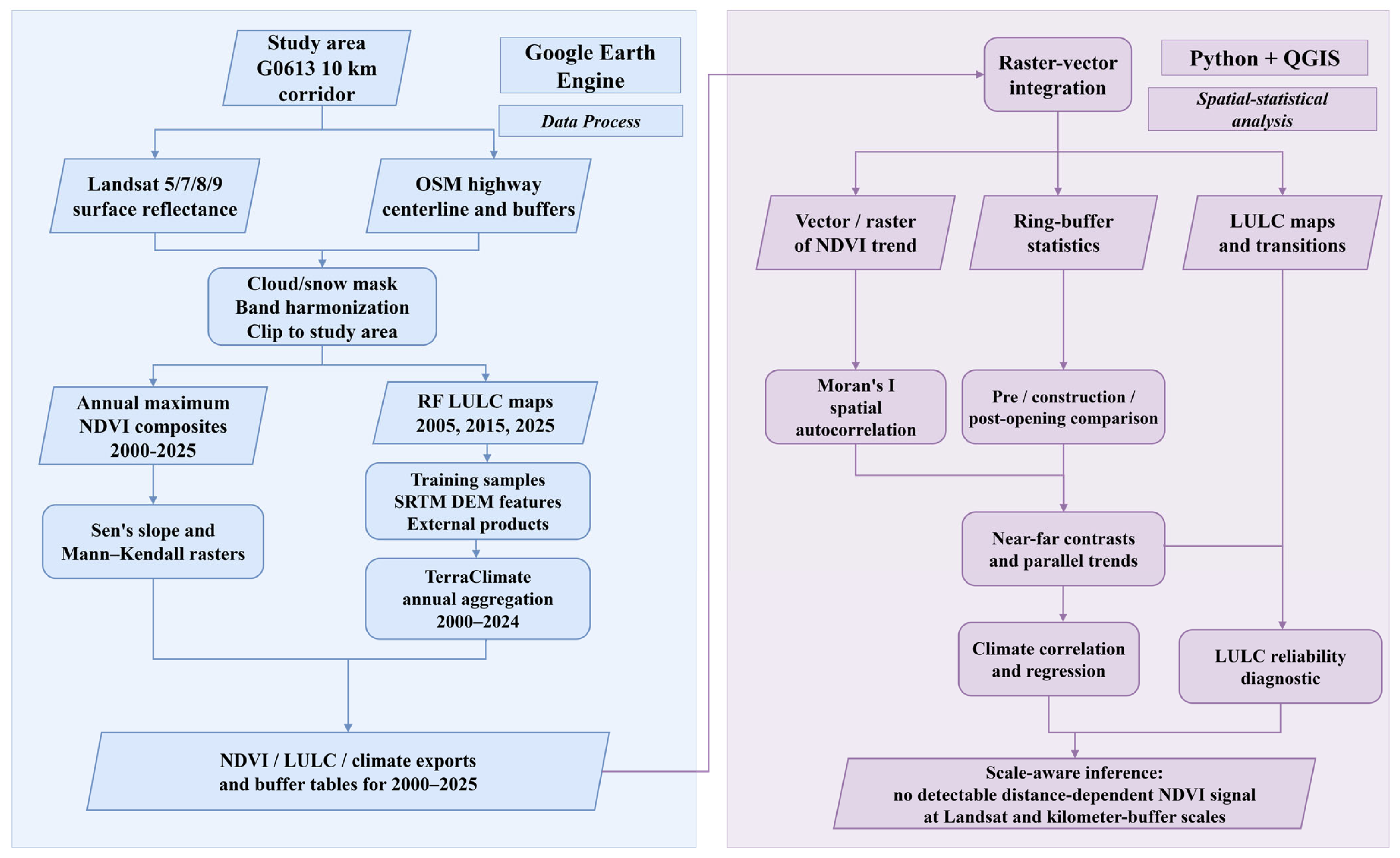
An overview of the data-processing and analysis workflow is shown in Figure 2. The workflow integrates Google Earth Engine-based preprocessing of Landsat, LULC, and climate datasets with subsequent raster-vector integration and spatial-statistical analyses in Python and QGIS. This structure was designed to evaluate whether a distance-dependent NDVI signal associated with the Gonghe-Yushu Expressway could be detected within the predefined 0–10 km corridor, while explicitly considering spatial autocorrelation, buffer-scale sensitivity, LULC reliability, and climate co-variation.

4. Results

4.1. Spatiotemporal Patterns of NDVI Change (2000–2025)

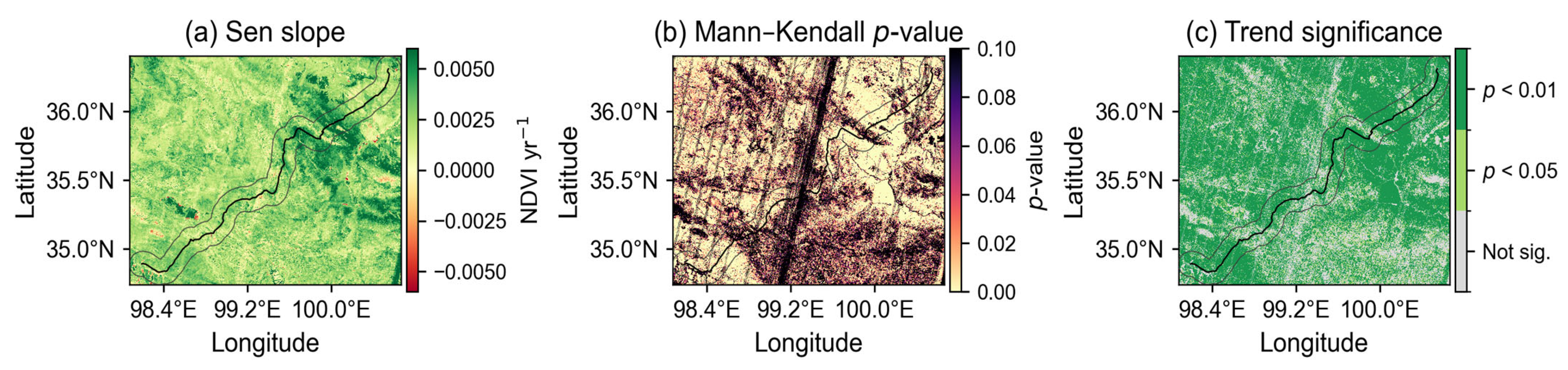
The Sen’s slope analysis revealed a widespread greening trend along the Gonghe-Yushu Expressway corridor over the 25-year study period (Figure 3). The mean NDVI slope was +0.0026 per year across the study area. Of the total valid pixels, 65.9% exhibited a highly significant increasing trend (p < 0.01), 11.4% showed a significant increase (0.01 < p < 0.05), and 22.8% showed no significant trend. Notably, no significant decreasing trends were detected in any part of the study area (Table 1). Annual valid corridor pixels were highly stable across the multi-sensor Landsat record, with a median of 9,096,788 valid pixels and a minimum valid fraction of 0.99 relative to the maximum annual count, suggesting that the mapped greening was not driven by changing raster coverage.
The spatial pattern of greening was relatively uniform across the corridor, with no obvious distance-dependent gradient from the highway (Figure 2). Both proximal (0–1 km) and distal (5–10 km) buffer zones exhibited comparable greening rates (Table 2), suggesting that the observed vegetation recovery was a regional phenomenon rather than a road-specific effect.

4.2. NDVI Dynamics Relative to Highway Construction

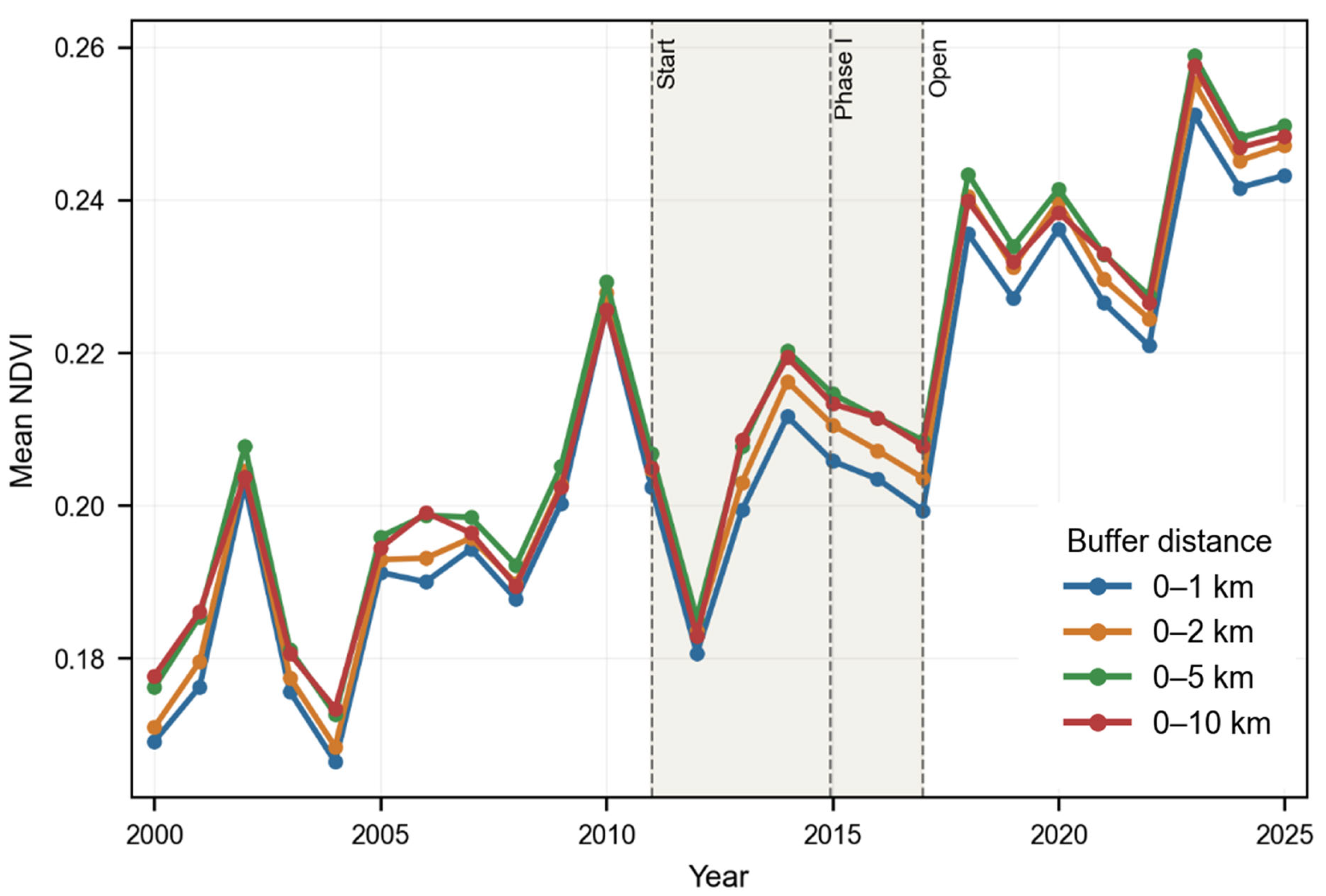
The temporal analysis of mean NDVI across the study area revealed a continuous upward trend that began well before the highway construction period (Figure 4). The mean NDVI in the 10 km buffer zone increased from approximately 0.35 in 2000 to 0.42 in 2025. Importantly, the greening trend was already established during the pre-construction period (2000–2011), with no detectable acceleration or deceleration associated with the construction phase (2011–2017, with the first phase completed in December 2014) or the post-construction operational period (2017–2025).
To examine whether the highway construction had a detectable impact on vegetation, we compared NDVI trends across three sub-periods: pre-construction (2000–2011), construction (2011–2017), and post-construction (2017–2025). The greening rate was consistent across all sub-periods, with slopes of +0.00267 NDVI/year (p = 0.017) for pre-construction, +0.00252 NDVI/year (p = 0.287, n = 7) for construction, and +0.00372 NDVI/year (p = 0.034) for post-construction (Table 3). The construction period slope was not statistically significant, likely due to the short time series (7 years) rather than an absence of trend. The post-construction period showed a slightly higher greening rate, but the difference was not statistically distinguishable given the overlapping confidence intervals. These results indicate that the highway construction did not produce a detectable disruption in the regional NDVI trajectory.

4.3. Land Use/Land Cover Changes

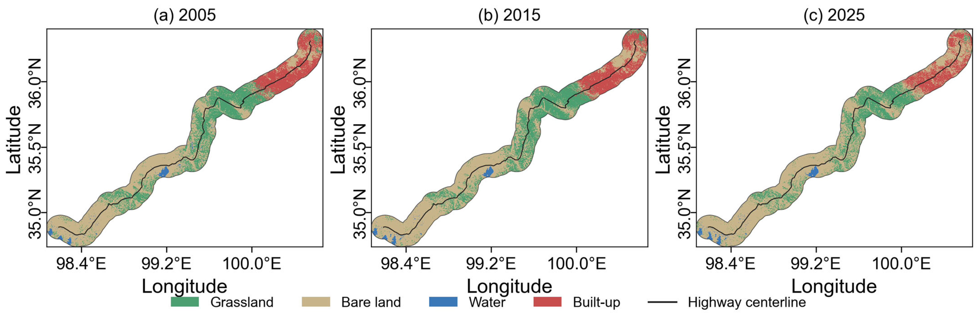
The LULC classification achieved high OOB accuracy estimates for all three periods, with OA values ranging from 0.9828 to 0.9943 and Kappa coefficients from 0.9765 to 0.9922 (Table 4; Figure 5). These OOB estimates indicate strong internal separability among the selected training samples and four target classes. However, these values reflect training-sample separability rather than the overall thematic accuracy of the final LULC maps and are not equivalent to independent external validation. Within the 10 km buffer corridor, Bare land was the dominant class (53.8–63.1%), followed by Grassland (23.2–28.5%), Built-up land (11.9–15.7%), and Water bodies (1.7–1.9%). The predominance of Bare land reflects the high-altitude plateau landscape where exposed soil and sparse vegetation are common, particularly along ridgelines and in rain shadow areas. The unusually high Built-up proportion (11.9–15.7% within the buffer versus 1.8–2.4% in the full Landsat scene) warrants caution: 100% of Built-up-classified pixels fell within the buffer corridor, indicating that the classifier captured the highway pavement, gravel shoulders, and associated infrastructure as a coherent spectral class. Some bare rock and exposed soil near the road may also have been misclassified as Built-up due to spectral similarity at 30 m resolution. The Built-up area statistics should therefore be interpreted as an upper-bound estimate of infrastructure footprint rather than a precise land use measurement.
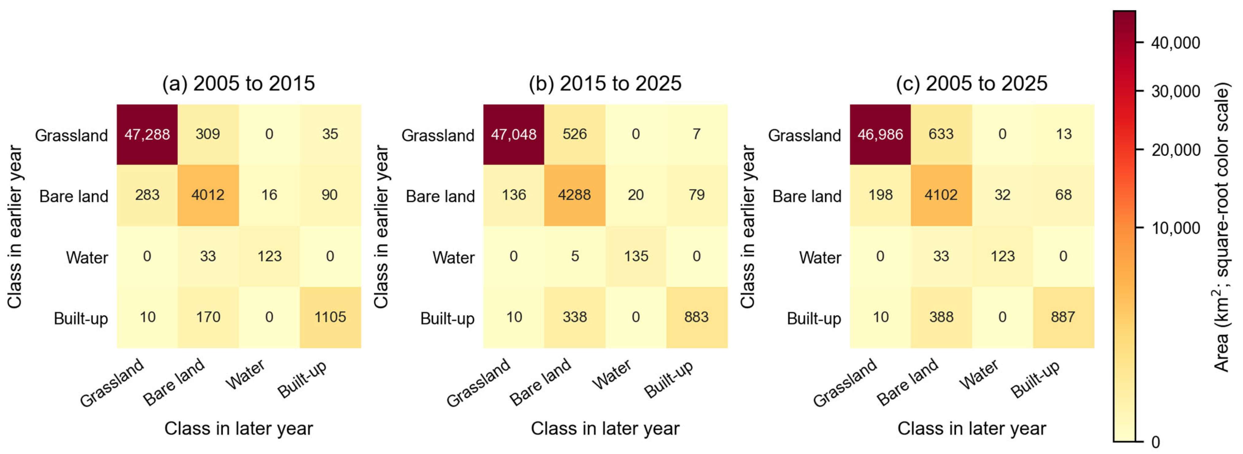
The transition matrix analysis (Table 5, Figure 6) revealed that inter-class transitions were limited in magnitude. The dominant transitions over 2005–2025 were: (1) Grassland to Bare land (633 km2), and (2) Built-up to Bare land (388 km2). These two transitions together account for 1021 km2, offset in part by reverse transitions (Bare land to Grassland: 198 km2; Bare land to Built-up: 68 km2). The net increase in Bare land area (+755 km2) was primarily at the expense of Grassland. Given the classification uncertainty and lack of independent validation, these transition magnitudes should be regarded as approximate landscape-level estimates rather than precise measurements of land-cover change.

4.4. Relationship Between NDVI and Climate Factors

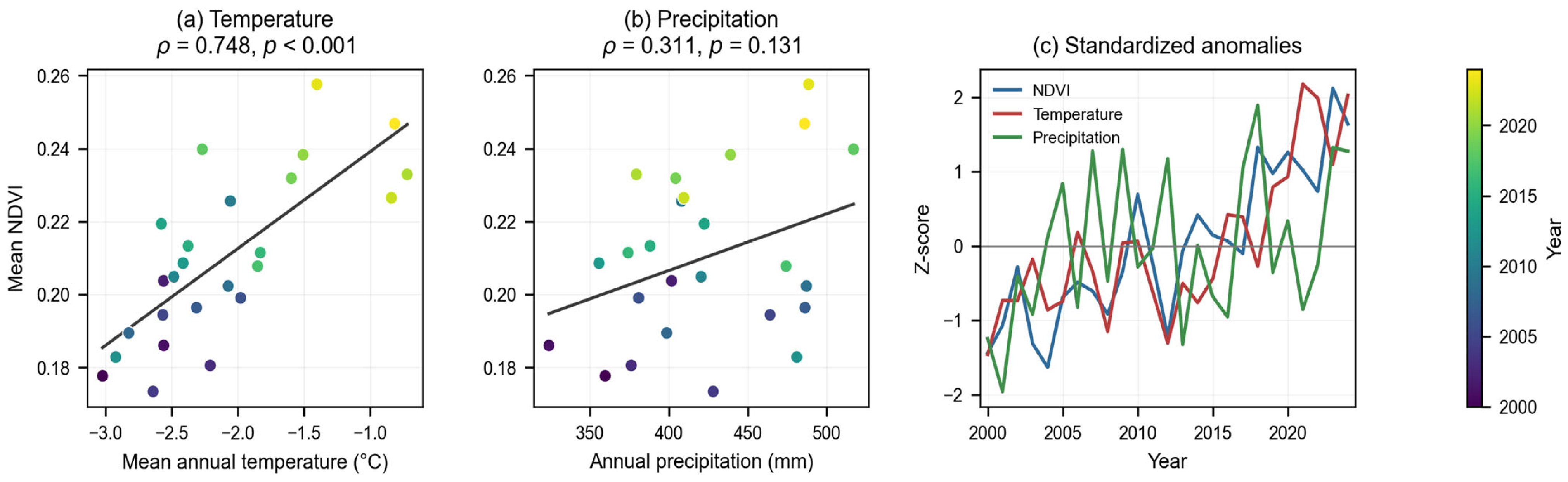
The correlation analysis between annual mean NDVI and climate variables (2000–2024, 25 years; TerraClimate data available through 2024 only) revealed a strong positive association with temperature and a weaker association with precipitation (Figure 7. The Spearman rank correlation coefficient between NDVI and mean annual temperature was ρ = 0.748 (p < 0.001), while the correlation with annual precipitation was ρ = 0.311 (p = 0.131, not significant at α = 0.05). Pearson correlations yielded similar results (r = 0.748, p < 0.001 for temperature; r = 0.347, p = 0.089 for precipitation), and Shapiro-Wilk tests confirmed normal distribution of all variables (p > 0.05). The buffer-level TerraClimate consistency diagnostic showed limited climate variation among the 1, 2, 5, and 10 km buffers. Across years, the mean annual temperature range among buffers averaged 0.263 °C, and the mean annual precipitation range averaged 5.41 mm. These small inter-buffer differences indicate that TerraClimate mainly represents the shared regional climate background of the corridor, rather than fine-scale roadside climatic gradients.
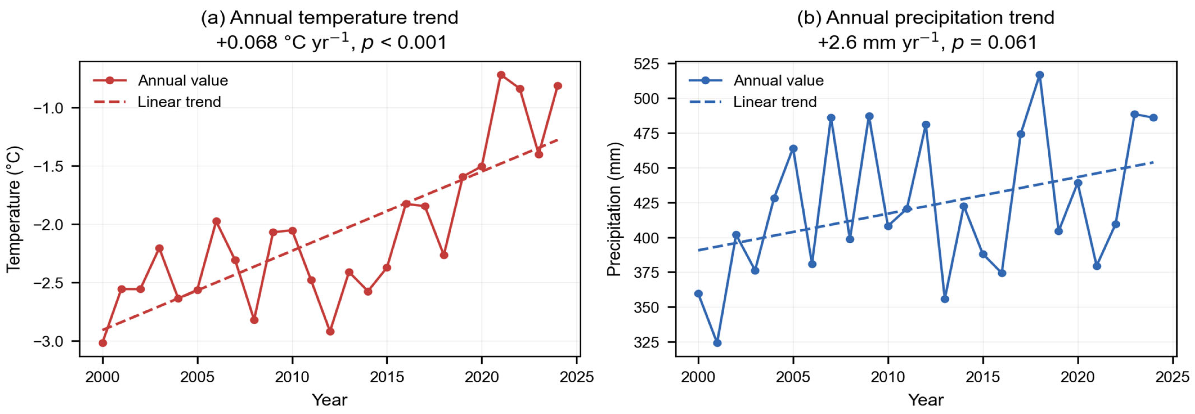
The sensitivity analyses further showed that the NDVI-temperature relationship remained strong after controlling for precipitation (partial r = 0.752, p < 0.001), but weakened after controlling for year (partial r = 0.243, p = 0.241). When both precipitation and year were controlled, the partial correlation between NDVI and temperature was also not significant (partial r = 0.262, p = 0.206). In standardized regression, temperature and precipitation explained 61.9% of annual NDVI variance. However, after year was added to the model, the standardized temperature coefficient decreased from 0.713 to 0.213, while the year coefficient was 0.680. These results indicate that temperature co-varied with the regional greening trend, but the simple NDVI-temperature correlation should not be interpreted as independent causal attribution. The climate trend analysis (2000–2024) showed a significant warming trend of +0.068 °C per year (p < 0.001), corresponding to approximately +1.7 °C over 25 years. The precipitation trend was positive (+2.63 mm/year) but not statistically significant (p = 0.062). The annual climate trajectories underlying these correlations are summarized in Figure 8.
Figure 8 provides the climate-context evidence behind the NDVI-climate correlations. Mean annual temperature shows a clear and sustained increase across the corridor, rising by approximately 1.7 degrees C over 2000–2024, whereas annual precipitation fluctuates strongly from year to year and only shows a weak, statistically non-significant upward tendency. This contrast indicates that the long-term greening signal is more consistent with a persistent thermal relaxation of cold-limited alpine vegetation than with a monotonic precipitation-driven response.
The strong coupling between NDVI and temperature, combined with the consistent greening across all buffer zones, suggests that climate warming is the primary correlate of vegetation recovery in this alpine region. The warming trend may promote vegetation growth through extended growing seasons, increased soil nutrient availability from permafrost thaw, and enhanced moisture conditions in previously cold-limited environments.

4.5. NDVI Gradient Analysis

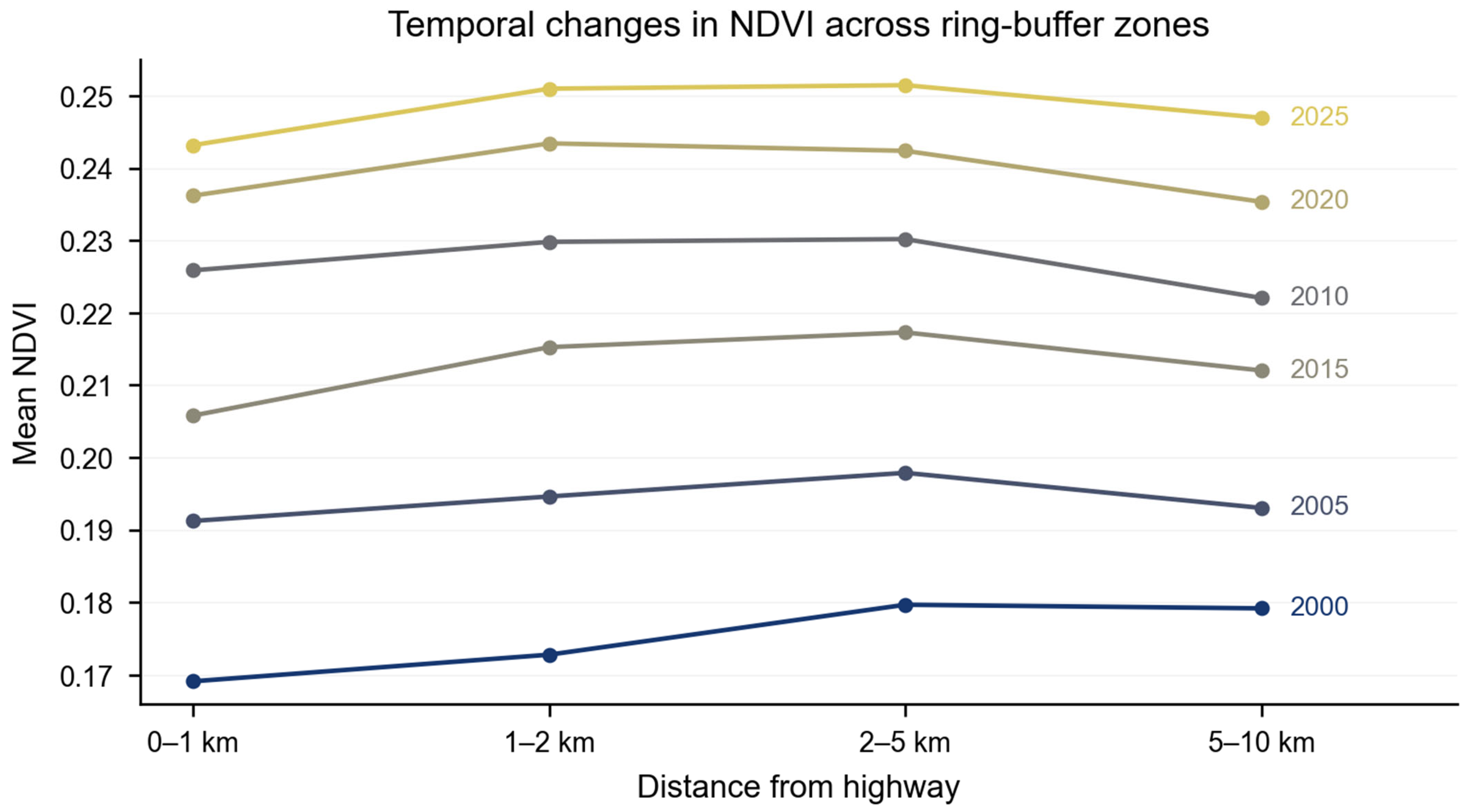
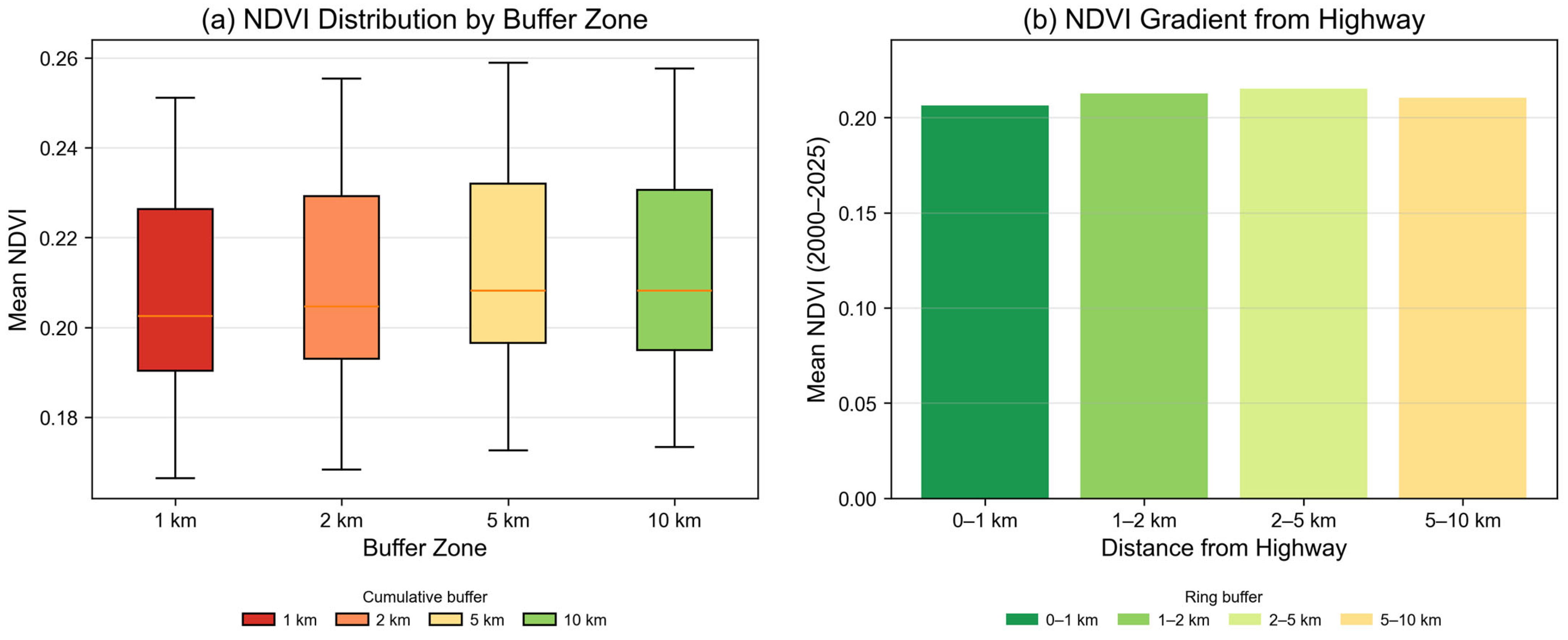
The ring buffer analysis (0–1, 1–2, 2–5, 5–10 km) revealed a subtle NDVI gradient, with slightly higher NDVI values in the 2–5 km zone compared to the immediate roadside (0–1 km) (Figure 9). However, this gradient was small (difference < 0.02 NDVI units) and remained stable throughout the study period, with no evidence of increasing divergence after highway construction. The temporal evolution of the gradient showed that all distance zones experienced parallel greening trajectories, further supporting the interpretation of a climate-driven regional signal rather than a road-disturbance effect. The ring-buffer sensitivity assessment showed similar NDVI trends across all distance zones. The 0–1, 1–2, 2–5, and 5–10 km rings had slopes of +0.00271, +0.00291, +0.00273, and +0.00270 NDVI/year, respectively. Near-far contrasts were small: −0.0039 NDVI for 0–1 km minus 5–10 km, +0.0023 for 1–2 km minus 5–10 km, and +0.0048 for 2–5 km minus 5–10 km. Period comparisons did not show a robust post-construction divergence among rings. All distance zones exhibited parallel greening trajectories, and no persistent distance-dependent highway-associated NDVI signal was detected.
Figure 10 complements the selected-year distance gradient in Figure 8 by summarizing the full buffer-zone distributions and annual trend behavior. The near-road zone and the outer reference zones overlap strongly in their NDVI distributions, and their annual trajectories rise in parallel rather than diverging after construction. This pattern supports the interpretation that kilometer-scale NDVI change is dominated by a regional greening signal; it does not rule out very narrow roadside impacts, but it indicates that such impacts are not expressed as a persistent buffer-scale gradient.

5. Discussion

5.1. Climate Warming as a Regional Correlate of Greening

The dominant finding of this study is a widespread and statistically significant greening trend along the Gonghe-Yushu Expressway corridor, with 77.3% of pixels showing significant NDVI increases over 2000–2025 and no significant decreasing trends detected. Accordingly, the pixel-wise Mann–Kendall significance maps should be interpreted as representations of spatially coherent trend patterns rather than as independent statistical tests for individual pixels. This greening pattern is strongly correlated with the regional warming trend (+0.068 °C/year), while precipitation changes played a minor role. These findings are consistent with previous studies that reported widespread vegetation greening across the QXP and linked vegetation trends to climatic factors and human activities [10,11,12,14,26].
The mechanism underlying the temperature-vegetation relationship in alpine ecosystems is well established. Warming temperatures can alter plant phenology and reproductive success, change the length and timing of the growing season, and interact with frozen-ground dynamics that influence alpine vegetation responses [27,28]. In the study region, where mean annual temperatures range from approximately −4 °C to 3 °C, even modest warming can substantially affect vegetation growth by pushing thermal conditions closer to the optimum for alpine meadow species. The absence of a significant precipitation signal suggests that temperature, rather than moisture, is the limiting factor for vegetation growth in this high-altitude environment, consistent with the energy-limited regime characteristic of the northeastern QXP [29]. Nevertheless, the weakened relationship after controlling for year indicates shared long-term co-variation rather than an independent climatic effect; warming is therefore regarded as the strongest observed correlate, while other environmental and land-management processes may also contribute.

5.2. Limited Detectable Impact of Highway Construction

A key finding of this study is that the Gonghe-Yushu Expressway construction (first phase completed December 2014, full opening August 2017) did not produce a statistically distinguishable change in the regional NDVI trajectory. The greening trend was already established during the pre-construction period (2000–2011), and no acceleration, deceleration, or spatial disruption was associated with the construction (2011–2017) or post-construction operational (2017–2025) phases. Furthermore, the buffer zone analysis revealed no meaningful distance-dependent gradient—all buffer zones (0–1, 1–2, 2–5, 5–10 km) exhibited comparable greening rates (Table 2). However, because this study lacks an independent control corridor and a formal BACI design, the appropriate interpretation is that no persistent distance-dependent NDVI signal was detectable at the analyzed Landsat and kilometer-buffer scales, not that localized highway impacts were absent.
This finding contrasts with earlier transport-corridor studies on the QXP that detected localized vegetation or biophysical changes near the Qinghai-Tibet Railway and Highway [5,6]. Several factors may explain this discrepancy. First, the Gonghe-Yushu Expressway was designed and constructed with more stringent environmental protection standards than earlier roads, potentially including measures such as vegetation restoration on disturbed slopes, wildlife corridors, and permafrost-protective road foundations. Second, the regional greening signal driven by climate warming may have overwhelmed any localized road-disturbance effect at the 30 m Landsat resolution. Third, the 10 km buffer analysis may be too coarse to detect narrow roadside impacts, which often occur within short distances from the road edge [7,17]. Therefore, the absence of a detectable buffer-scale NDVI signal should not be interpreted as evidence that localized roadside impacts were absent. Narrower buffers and higher-resolution imagery may reveal localized patterns that cannot be resolved within the current Landsat-based framework.
The LULC transition analysis provides contextual information on broad land-cover conditions. Within the 10 km buffer corridor, the dominant land cover transitions over 2005–2025 were Grassland to Bare land (633 km2) and Built-up to Bare land (388 km2), which are likely driven by natural variability (e.g., drought years, grazing pressure) rather than road construction. The apparent decrease in Built-up area (−317 km2) is likely an artifact of spectral confusion between Built-up and Bare land classes at 30 m resolution, rather than actual urbanization decline. The concentration of all Built-up pixels within the buffer corridor (100% of the scene total) further suggests that the classifier captured highway-associated surfaces (pavement, gravel, infrastructure) rather than distributed urban land use, and that some bare rocky areas near the road may have been misclassified. Accordingly, the reported LULC changes are interpreted as approximate contextual estimates.

5.3. Comparison with Other QXP Road Ecology Studies

The greening rate observed in this study (+0.0026 NDVI/year) is comparable to reported trends for other parts of the QXP. Piao et al. [10] reported a mean NDVI increase of approximately 0.002/year for China’s temperate vegetation over 1982–2002, while recent QXP-scale remote sensing studies have reported overall greening during the MODIS and Landsat eras [11,12]. The greening rate in the Gonghe-Yushu corridor falls within this broader pattern, suggesting that this region is experiencing vegetation recovery consistent with the wider QXP trend.
The absence of a road-disturbance signal in our study differs from some findings along the Qinghai-Xizang Railway, where vegetation abundance changes were most evident close to the track during the construction period [5]. It is also consistent with more recent evidence that transport-related biophysical effects on the QXP can be spatially heterogeneous and may not form a clear gradient with increasing distance from transport lines [6]. This difference may reflect: (1) the older construction history of the railway versus the expressway; (2) different construction techniques and environmental mitigation measures; or (3) the wider corridor analysis (1–10 km) used in this study, which may dilute narrow roadside effects.

5.4. Implications for Road Ecology and Conservation

The results of this study have two important implications. First, no persistent highway-associated vegetation degradation pattern was detectable at the analyzed Landsat and kilometer-buffer scales. The regional greening associated with climate warming may have masked or compensated for any localized construction disturbance at the spatial resolution used in this study. This suggests that modern highway construction practices in China, combined with the regional greening trend, may reduce the detectability of road-related ecological impacts over decadal timescales.
Second, the strong temperature-vegetation coupling identified in this study highlights the vulnerability of these ecosystems to future climate change. While current warming has promoted vegetation growth, continued warming could eventually exceed the thermal optimum for alpine meadow species, leading to potential degradation or altered phenological and reproductive responses [27,28]. Additionally, permafrost thaw associated with warming could destabilize road foundations and alter surface hydrology, creating new ecological challenges in the coming decades.

5.5. Limitations

This study has several limitations that should be acknowledged. First, the 30 m Landsat resolution may not reliably capture fine-scale roadside vegetation changes occurring within narrow corridors, especially effects associated with embankments, drainage structures, restoration slopes, construction footprints, roadside strips, or mixed pavement-gravel-bare soil surfaces. Although Collection 2 surface reflectance products, QA_PIXEL masking, band harmonization, annual maximum compositing, and valid-pixel diagnostics were used to improve temporal consistency, residual cross-sensor differences, Landsat 7 SLC-off effects, and phenological sampling uncertainty cannot be fully eliminated. Higher-resolution imagery (e.g., Sentinel-2 at 10 m, or sub-meter commercial imagery) would be needed to detect localized road effects. Second, the LULC classification was limited to four classes due to insufficient training samples for Wetland and Glacier/Snow categories, which may have obscured important land cover transitions in these ecologically sensitive types. Third, the training samples (n = 174) were derived from spectral rules and visual verification against high-resolution imagery rather than field surveys, potentially introducing systematic bias. The small sample size, particularly for Water body (n = 24), limits the statistical robustness of per-class accuracy estimates. Moreover, the 174 training samples distributed across the extensive 10 km buffer corridor may not fully capture the environmental heterogeneity of the study area. Fourth, the LULC accuracy assessment used Random Forest OOB estimation as the primary internal accuracy metric. Although OOB estimates are useful for internal model assessment, they may be optimistic when training samples are limited or spatially autocorrelated; independent field or visual validation would further strengthen future versions of the classification product [25]. Fifth, the climate analysis relied on TerraClimate data at ~4 km resolution (available through 2024 only), which may not adequately represent local microclimatic variations in the complex terrain of the study area. TerraClimate provides useful regional climate context, but it was not independently validated against dense in-situ meteorological observations within the corridor; therefore, climate-related results should be interpreted as regional co-variation rather than local causal attribution. Sixth, the study does not include an independent control corridor or a formal BACI design, so it cannot fully separate highway-related effects from broader regional greening trends. Seventh, the Mann-Kendall analyses did not explicitly correct for serial autocorrelation; future work could apply modified Mann-Kendall or pre-whitening approaches to test the robustness of trend significance [30].

6. Conclusions

This study conducted a comprehensive analysis of vegetation dynamics and land cover changes along the Gonghe-Yushu Expressway corridor on the northeastern Qinghai-Xizang Plateau from 2000 to 2025 using 25 years of Landsat imagery and climate data. The main conclusions are as follows:
(1)
A widespread and statistically significant greening trend was detected across the study area, with 77.3% of pixels showing significant NDVI increases and no significant decreasing trends. The mean greening rate was +0.0026 NDVI per year over the 25-year period.
(2)
The greening trend was established before the highway construction (first phase completed December 2014, full opening August 2017) and continued uniformly through the construction and post-construction periods. No statistically distinguishable impact of highway construction on regional NDVI trajectories was detected.
(3)
The LULC classification showed that Bare land and Grassland were the dominant classes within the 10 km buffer corridor, with limited inter-class transitions. Bare land area increased by 17.2% (+755 km2), primarily at the expense of Grassland, while other classes remained relatively stable.
(4)
Climate warming (+0.068 °C/year) was associated with vegetation greening, as evidenced by the strong positive correlation between NDVI and temperature (ρ = 0.748, p < 0.001). Precipitation changes showed no significant correlation with NDVI. This association should be interpreted as long-term co-variation rather than evidence of an independent climatic driving mechanism.
(5)
Within the predefined 0–10 km study corridor at 30 m Landsat resolution, the buffer-zone sensitivity analysis revealed no persistent distance-dependent NDVI divergence among the 0–1, 1–2, 2–5, and 5–10 km rings. However, the absence of a detectable response at 30 m resolution does not exclude localized ecological impacts that cannot be resolved within the current Landsat-based framework.
These findings indicate that the Gonghe-Yushu Expressway corridor has not experienced the vegetation degradation typically associated with highway construction in alpine environments. The absence of detectable road-associated vegetation change, combined with strong climate-driven greening, suggests that either construction impacts were minimal at the spatial and temporal scales examined, or they were masked by the dominant regional greening signal. Future work should use independent reference corridors, higher-resolution imagery, narrower roadside buffers, field or high-resolution visual validation, and ancillary grazing/restoration data to better evaluate localized highway effects.

Author Contributions

Author Contributions: Conceptualization, K.Z. and Y.M.; methodology, K.Z., Y.M. and Z.D.; software, K.Z., Y.M. and Z.D.; validation, K.Z., Y.M. and Z.D.; formal analysis, K.Z., Y.M. and Z.D.; investigation, K.Z., Y.M. and Z.D.; resources, K.Z., Y.M. and Z.D.; data curation, K.Z., Y.M. and Z.D.; writing—original draft preparation, K.Z., Y.M. and Z.D.; writing—review and editing, K.Z., Y.M. and Z.D.; visualization, Y.S. and L.L.; supervision, K.Z., Y.M. and Z.D.; project administration, K.Z., Y.M. and Z.D. All authors have read and agreed to the published version of the manuscript.

Funding

This research was supported by the Talent Project of Northwest Minzu University (No. xbmuyjrc2023018), the Gansu Provincial Natural Science Foundation (No. 25JRRA995), the Science and Technology Program of Gansu Province (No. 23ZDFA017), and the Science and Technology Program of Gansu Province (Nos. 25JRRA535 and 24JRRA099).

Data Availability Statement

The satellite, terrain, and climate datasets used in this study are publicly available from the Google Earth Engine data catalog, including Landsat Collection 2 Level-2 surface reflectance products, SRTM DEM, and TerraClimate. OpenStreetMap data were used to delineate the highway centerline. Derived analysis code and processed tabular outputs should be deposited in a public repository before submission; until deposition, they are available from the corresponding author upon reasonable request.

Acknowledgments

We thank the anonymous reviewers for their insightful and constructive comments on this manuscript. We also thank the editor and the associate editor for their invaluable help on our manuscript.

Conflicts of Interest

The authors declare no conflict of interest.

References

  1. Qiu, J. China: The third pole. Nature 2008, 454, 393–396. [Google Scholar] [CrossRef] [Scilit] [PubMed]
  2. Yao, T.; Thompson, L.; Yang, W.; Yu, W.; Gao, Y.; Guo, X.; Yang, X.; Duan, K.; Zhao, H.; Xu, B.; et al. Different glacier status with atmospheric circulations in Tibetan Plateau and surroundings. Nat. Clim. Change 2012, 2, 663–667. [Google Scholar] [CrossRef] [Scilit]
  3. Cui, X.; Graf, H.F. Recent land cover changes on the Tibetan Plateau: A review. Clim. Change 2009, 94, 47–61. [Google Scholar] [CrossRef] [Scilit]
  4. Yang, S.; Zhang, L.; Zhu, G. Effects of transport infrastructures and climate change on ecosystem services in the integrated transport corridor region of the Qinghai-Tibet Plateau. Sci. Total Environ. 2023, 885, 163961. [Google Scholar] [CrossRef] [Scilit] [PubMed]
  5. Wang, G.; Gillespie, A.R.; Liang, S.; Mushkin, A.; Wu, Q. Effect of the Qinghai-Tibet Railway on vegetation abundance. Int. J. Remote Sens. 2015, 36, 5222–5238. [Google Scholar] [CrossRef] [Scilit]
  6. Zhou, D.; Zhang, L.; Huang, L.; Fan, J.; Li, Y.; Zhang, H. Satellite evidence for small biophysical effects of transport infrastructure in the Qinghai-Xizang Plateau. J. Clean. Prod. 2023, 416, 138002. [Google Scholar] [CrossRef] [Scilit]
  7. Forman, R.T.T.; Alexander, L.E. Roads and their major ecological effects. Annu. Rev. Ecol. Syst. 1998, 29, 207–231. [Google Scholar] [CrossRef] [Scilit]
  8. Trombulak, S.C.; Frissell, C.A. Review of ecological effects of roads on terrestrial and aquatic communities. Conserv. Biol. 2000, 14, 18–30. [Google Scholar] [CrossRef] [Scilit]
  9. Pettorelli, N.; Vik, J.O.; Mysterud, A.; Gaillard, J.M.; Tucker, C.J.; Stenseth, N.C. Using the satellite-derived NDVI to assess ecological responses to environmental change. Trends Ecol. Evol. 2005, 20, 503–510. [Google Scholar] [CrossRef] [Scilit] [PubMed]
  10. Piao, S.; Fang, J.; Zhou, L.; Ciais, P.; Zhu, B. Variations in satellite-derived phenology in China’s temperate vegetation. Glob. Change Biol. 2006, 12, 672–685. [Google Scholar] [CrossRef] [Scilit]
  11. Song, Y.; Jin, L.; Wang, H. Vegetation changes along the Qinghai-Xizang Plateau Engineering Corridor since 2000 induced by climate change and human activities. Remote Sens. 2018, 10, 95. [Google Scholar] [CrossRef] [Scilit]
  12. Chang, Y.; Yang, C.; Xu, L.; Li, D.; Shang, H.; Gao, F. Analysis of vegetation dynamics and driving mechanisms on the Qinghai-Xizang Plateau in the context of climate change. Water 2023, 15, 3305. [Google Scholar] [CrossRef] [Scilit]
  13. Zhou, G.; Ren, H.; Zhang, L.; Lv, X.; Zhou, M. Annual vegetation maps in the Qinghai-Tibet Plateau (QTP) from 2000 to 2022 based on MODIS series satellite imagery. Earth Syst. Sci. Data 2025, 17, 773–797. [Google Scholar] [CrossRef] [Scilit]
  14. Wang, H.; Zhan, J.; Wang, C.; Liu, W.; Yang, Z.; Liu, H.; Bai, C. Greening or browning? The macro variation and drivers of different vegetation types on the Qinghai-Tibetan Plateau from 2000 to 2021. Front. Plant Sci. 2022, 13, 1045290. [Google Scholar] [CrossRef] [Scilit] [PubMed]
  15. Sen, P.K. Estimates of the regression coefficient based on Kendall’s tau. J. Am. Stat. Assoc. 1968, 63, 1379–1389. [Google Scholar] [CrossRef]
  16. Belgiu, M.; Drăguţ, L. Random forest in remote sensing: A review. ISPRS J. Photogramm. Remote Sens. 2016, 114, 24–31. [Google Scholar] [CrossRef] [Scilit]
  17. Forman, R.T.T.; Deblinger, R.D. The ecological road-effect zone of a Massachusetts (U.S.A.) suburban highway. Conserv. Biol. 2000, 14, 36–46. [Google Scholar] [CrossRef] [Scilit]
  18. Zhang, L.; Miao, Y.; Wei, H.; Dai, T. Ecological impacts associated with the Qinghai-Tibet Railway and its influencing factors: A comparison study on diversified research units. Int. J. Environ. Res. Public Health 2023, 20, 4154. [Google Scholar] [CrossRef] [Scilit] [PubMed]
  19. Guo, L.; Li, Y.; Luo, Y.; Gao, J.; Zhang, H.; Zou, Y.; Wu, S. The compound effects of highway reconstruction and climate change on vegetation activity over the Qinghai Tibet Plateau: The G318 Highway as a case study. Remote Sens. 2023, 15, 5473. [Google Scholar] [CrossRef] [Scilit]
  20. Earth Resources Observation and Science (EROS) Center. Landsat Collection 2. U.S. Geological Survey Fact Sheet 2021–3002; U.S. Geological Survey: Reston, VA, USA, 2021. [Google Scholar] [CrossRef] [Scilit]
  21. Gorelick, N.; Hancher, M.; Dixon, M.; Ilyushchenko, S.; Thau, D.; Moore, R. Google Earth Engine: Planetary-scale geospatial analysis for everyone. Remote Sens. Environ. 2017, 202, 18–27. [Google Scholar] [CrossRef] [Scilit]
  22. Abatzoglou, J.T.; Dobrowski, S.Z.; Parks, S.A.; Hegewisch, K.C. TerraClimate, a high-resolution global dataset of monthly climate and climatic water balance from 1958–2015. Sci. Data 2018, 5, 170191. [Google Scholar] [CrossRef] [Scilit] [PubMed]
  23. Mann, H.B. Nonparametric tests against trend. Econometrica 1945, 13, 245–259. [Google Scholar] [CrossRef] [Scilit]
  24. Sun, N.; Chen, Q.; Liu, F.; Zhou, Q.; He, W.; Guo, Y. Land use simulation and landscape ecological risk assessment on the Qinghai-Xizang Plateau. Land 2023, 12, 923. [Google Scholar] [CrossRef] [Scilit]
  25. Olofsson, P.; Foody, G.M.; Herold, M.; Stehman, S.V.; Woodcock, C.E.; Wulder, M.A. Good practices for estimating area and assessing accuracy of land change. Remote Sens. Environ. 2014, 148, 42–57. [Google Scholar] [CrossRef] [Scilit]
  26. Yang, J.; Xin, Z.; Huang, Y.; Liang, X. Multi-source remote sensing data shows a significant increase in vegetation on the Tibetan Plateau since 2000. Prog. Phys. Geogr. Earth Environ. 2023, 47, 597–624. [Google Scholar] [CrossRef] [Scilit]
  27. Dorji, T.; Totland, Ø.; Moe, S.R.; Hopping, K.A.; Pan, J.; Klein, J.A. Plant functional traits mediate reproductive phenology and success in response to experimental warming and snow addition in Tibet. Glob. Change Biol. 2013, 19, 459–472. [Google Scholar] [CrossRef] [Scilit] [PubMed]
  28. Luo, L.; Ma, W.; Zhuang, Y.; Zhang, Y.; Yi, S.; Xu, J.; Long, Y.; Ma, D.; Zhang, Z. The impacts of climate change and human activities on alpine vegetation and permafrost in the Qinghai-Tibet Engineering Corridor. Ecol. Indic. 2018, 93, 24–35. [Google Scholar] [CrossRef] [Scilit]
  29. Shen, M.; Sun, Z.; Wang, S.; Zhang, G.; Kong, W.; Chen, A.; Piao, S. No evidence of continuously advanced green-up dates in the Tibetan Plateau over the last decade. Proc. Natl. Acad. Sci. USA 2013, 110, E2329–E2336. [Google Scholar] [CrossRef] [Scilit] [PubMed]
  30. Hamed, K.H.; Rao, A.R. A modified Mann-Kendall trend test for autocorrelated data. J. Hydrol. 1998, 204, 182–196. [Google Scholar] [CrossRef] [Scilit]
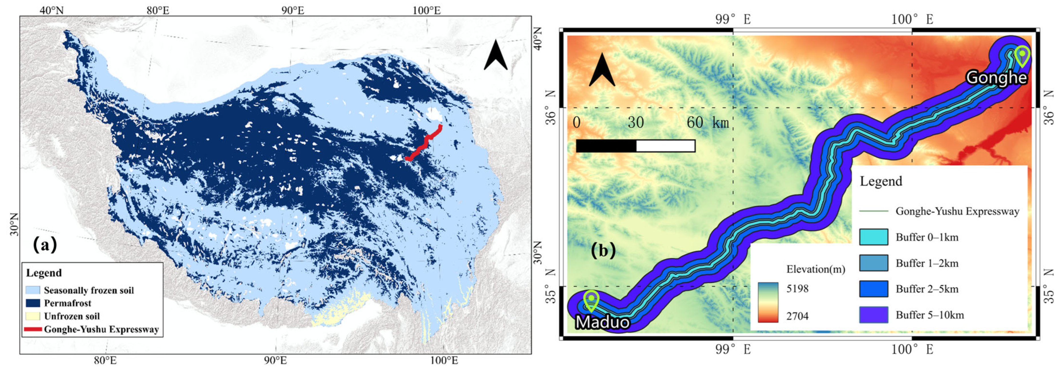
Figure 1. Regional context and study area of the Gonghe-Yushu Expressway (G0613) corridor in Qinghai Province, China. (a) Location of the Gonghe-Yushu Expressway on the Qinghai-Xizang Plateau in relation to seasonally frozen soil, permafrost, and unfrozen soil zones. (b) Study corridor showing SRTM DEM-derived elevation shading within the 10 km buffer, the highway centerline, and concentric ring buffer zones (0–1, 1–2, 2–5, and 5–10 km) from the centerline. Gonghe and Maduo are labeled as key reference locations along the mapped corridor.
Remotesensing 18 02354 g001
Figure 2. Methodological workflow for assessing vegetation dynamics and detectable distance-dependent NDVI signals along the Gonghe-Yushu Expressway corridor. Landsat surface reflectance, OpenStreetMap highway vectors, SRTM DEM, LULC training samples, external land-cover products, and TerraClimate data were processed in Google Earth Engine and then integrated with raster-vector and spatial-statistical analyses in Python 3.9 and QGIS 3.4. The workflow emphasizes ring-buffer statistics, spatial autocorrelation diagnostics, construction-period comparisons, near-far contrasts, climate correlation/regression analysis, and LULC reliability assessment.
Remotesensing 18 02354 g002
Figure 3. Spatial distribution of NDVI trends along the Gonghe-Yushu Expressway corridor (2000–2025). Sen’s slope values were classified by Mann-Kendall significance into highly significant increase (p < 0.01), significant increase (0.01 < p < 0.05), and not significant (p > 0.05). No significant decreasing trends were detected. The highway centerline is shown in black.
Remotesensing 18 02354 g003
Figure 4. Temporal evolution of mean NDVI in the 10 km buffer zone (2000–2025). The vertical dashed lines indicate the construction period: start of construction (2011), completion of first phase (December 2014), and full opening (August 2017). The green line shows the linear trend for the full period (slope = +0.00273 NDVI/year, R2 = 0.777, p < 0.001).
Remotesensing 18 02354 g004
Figure 5. Land use/land cover (LULC) classification maps for three representative periods: (a) 2005, (b) 2015, and (c) 2025. Four classes are shown: Grassland, Bare land, Water body, and Built-up land.
Remotesensing 18 02354 g005
Figure 6. LULC transition matrices for three periods: (a) 2005→2015, (b) 2015→2025, and (c) 2005→2025. Cell values represent transition areas in km2. Diagonal elements indicate persistence of each land cover class. The dominant off-diagonal transitions are Grassland to Bare land and Built-up to Bare land.
Remotesensing 18 02354 g006
Figure 7. Relationships between annual mean NDVI and climate variables (2000–2024). (a) NDVI vs. mean annual temperature (Spearman ρ = 0.748, p < 0.001). (b) NDVI vs. annual precipitation (Spearman ρ = 0.311, p = 0.131). (c) Standardized annual anomalies of NDVI, temperature, and precipitation, showing their temporal co-variation. Color scales in (a,b) indicate year.
Remotesensing 18 02354 g007
Figure 8. Annual temperature and precipitation trends from TerraClimate data for the 10 km buffer corridor.
Remotesensing 18 02354 g008
Figure 9. NDVI gradient across ring buffer zones (0–1, 1–2, 2–5, 5–10 km) for selected years. The gradient is small (<0.02 NDVI units) and remained stable throughout the study period, with no evidence of increasing divergence after highway construction. All distance zones experienced parallel greening trajectories.
Remotesensing 18 02354 g009
Figure 10. NDVI distributions and distance gradients across highway buffers. (a) Annual NDVI distributions within cumulative 1, 2, 5, and 10 km buffers; box colors identify the cumulative buffer extents. (b) Mean NDVI across non-overlapping 0–1, 1–2, 2–5, and 5–10 km ring buffers over 2000–2025; bar colors identify the ring-buffer distance classes.
Remotesensing 18 02354 g010
Table 1. Summary of NDVI trend classification based on Mann-Kendall test (2000–2025).
CategoryArea (%)
Highly significant increase (p < 0.01)65.9
Significant increase (0.01 < p < 0.05)11.4
Not significant (p > 0.05)22.8
Significant decrease (0.01 < p < 0.05)0.0
Highly significant decrease (p < 0.01)0.0
Table 2. NDVI trend slopes by buffer zone distance from the highway.
Buffer ZoneSlope (NDVI/Year)R2p-Value
0–1 km0.002710.745<0.001
1–2 km0.002810.760<0.001
2–5 km0.002760.762<0.001
5–10 km0.002730.777<0.001
Table 3. NDVI trend slopes by sub-period in the 10 km buffer zone.
Sub-PeriodYearsSlope (NDVI/Year)R2p-Value
Pre-construction2000–20110.002670.4500.017
Construction2011–20170.002520.2210.287
Post-construction2017–20250.003720.4970.034
Full period2000–20250.002730.777<0.001
Table 4. LULC classification accuracy estimates based on Random Forest OOB evaluation.
PeriodOAKappa
20050.99430.9922
20150.98280.9765
20250.99430.9922
Table 5. LULC area statistics within the 10 km buffer corridor for three periods (km2).
Class200520152025Change (2005–2025)
Grassland233222801893−439 (−18.8%)
Bare land440045235156+755 (+17.2%)
Water body156140155−1 (−0.6%)
Built-up12861230969−317 (−24.6%)
Total817481748174
Disclaimer/Publisher’s Note: The statements, opinions and data contained in all publications are solely those of the individual author(s) and contributor(s) and not of MDPI and/or the editor(s). MDPI and/or the editor(s) disclaim responsibility for any injury to people or property resulting from any ideas, methods, instructions or products referred to in the content.