Land Use/Land Cover Classification of the Qinghai Lake Basin Using Multitemporal Sentinel-1/2 Imagery

Highlights

What are the main findings?

• Integrating the seasonal optical and SAR data improved the classification accuracy.
• The QLBLC-10 Level-1 and Level-2 LULC datasets achieved apparent overall accuracies of 91.95% and 91.24%, and an area-weighted overall accuracy of 81.50% for Level-2.

What are the implications of the main findings?

• QLBLC-10 outperforms existing global and regional LULC datasets in representing alpine land cover patterns in the Qinghai Lake Basin.
• Provides a regionally adapted classification framework for LULC mapping in complex alpine ecosystems.

Abstract

The Qinghai Lake Basin (QLB) serves as a crucial ecological barrier on the Qinghai–Tibet Plateau, making high-precision mapping of land use/land cover (LULC) essential for eco-hydrological research within the basin. In this study, multitemporal Sentinel-1 radar and Sentinel-2 optical imagery from 2024, DEM-derived terrain information, and features derived from these sources were used to produce a 10-m resolution LULC map for the QLB using a support vector machine classifier. The Level-1 and Level-2 LULC datasets of QLB (QLBLC-10) achieved sample-based apparent overall accuracies (OAs) of 91.95% and 91.24%, respectively, and kappa coefficients of 0.90 for both. In contrast, the area-weighted apparent overall accuracy (OA_w) decreased to 81.50 ± 2.09% (95% confidence interval), indicating that class-area imbalance and small-area classes affect map-level performance. The ablation study confirms the contribution of multisource temporal information and terrain constraints to alpine LULC classification. The OA increased from 77.07% with single-temporal Sentinel-2 to 91.24% when multitemporal Sentinel-1/2 data and DEM-derived features were added, while the kappa coefficient increased from 0.75 to 0.90. The comparison with existing products shows that QLBLC-10 outperforms existing global and regional LULC datasets in representing alpine land cover patterns in the QLB. The LULC system proposed in this study is tailored to the QLB, and the presented LULC classification strategy enhances discrimination among major alpine vegetation types, including temperate and alpine steppes, alpine meadows, and alpine shrublands. It provides an up-to-date (2024) LULC dataset for ecosystem monitoring and land management across the QLB.

1. Introduction

The Qinghai Lake Basin (QLB), located on the northeastern Qinghai–Tibet Plateau (QTP), is a representative area with a high-elevation ecosystem [1]. The unique geographical position of the QLB dictates its importance in alpine eco-hydrological research. However, in recent years, climate change and human activities have accelerated grassland degradation and desertification in the QLB, driving significant changes in land use and land cover (LULC) patterns [2]. Meanwhile, current eco-hydrological studies and sustainable land management efforts are somewhat hindered by the lack of up-to-date, high-accuracy, and internally discriminative LULC datasets with fine spatial resolution.

A wide range of global and regional LULC datasets currently provide baseline information for the QLB [3,4]. Global 10-m products, such as ESA WorldCover, FROM-GLC10, GLC-FCS10, and Dynamic World, have been generated using Sentinel-1/2 imagery combined with machine learning or deep learning algorithms [5,6,7,8,9]. Regional mapping efforts on the QTP have produced valuable historical datasets, including 30-m regional maps [10] and 500-m MODIS-based vegetation series [11]. More recently, Li et al. developed the Tibetan Plateau Land Cover Dataset (TPLCD) at 30-m resolution from 1990 to 2023, with selected categories referencing the International Geosphere–Biosphere Program (IGBP) classification system [12]. However, despite their utility, most existing products adopt generalized classification schemes that are ill-equipped for alpine ecosystems. For example, the widely used IGBP scheme emphasizes detailed forest classifications, which are largely irrelevant to the grassland-dominated and highly heterogeneous landscapes of the QLB [13]. Consequently, establishing an alpine-adapted, high-resolution mapping strategy capable of resolving these grassland subtypes remains a critical gap.

Addressing this gap, however, is hindered by extreme environmental heterogeneity in alpine regions. Elevation, soil moisture, climatic variability, and phenological dynamics create a complex mosaic of spectrally similar vegetation, including temperate steppe, alpine steppe, alpine meadow, shrubland, and wetland [14,15]. This high inter-class similarity limits the capability of existing LULC products, making the fine-scale discrimination of alpine grassland subcategories a persistent scientific challenge. Recent advances have shown that integrating multisource and multitemporal data can effectively enhance LULC classification in complex landscapes [16,17]. While Sentinel-2 imagery provides rich spectral information [18,19], Sentinel-1 SAR offers all-weather sensitivity to vegetation structure and soil moisture [20]. Although their fusion generally improves class separability [5,21], how multisource information alleviates the classification challenges of alpine vegetation remains insufficiently explored. Furthermore, processing such high-dimensional fusion datasets requires robust supervised classifiers [22].

Supervised classification approaches—ranging from traditional machine learning techniques, such as random forests (RFs) and support vector machines (SVMs), to advanced ensemble methods (e.g., XGBoost and LightGBM) and deep-learning architectures—leverage labeled samples to achieve high accuracy [11,23,24]. While deep-learning and tree-based ensemble models have demonstrated remarkable representation capabilities, they generally require large training datasets and substantial computational resources. In contrast, SVMs exhibit strong generalization capabilities and maintain competitive accuracy under small training sample spaces, making them well-suited for the limited field samples typical of harsh alpine environments [25,26]. To address the above-mentioned challenges, in this work, we used SVMs to develop a high-accuracy and synergistic LULC mapping method tailored to alpine regions, and produced an up-to-date (2024) 10-m-resolution LULC dataset (QLBLC-10) at two classification levels (QLBLC-10-L1 and QLBLC-10-L2) by integrating seasonal optical data, SAR backscatter, and DEM features. The proposed approach demonstrates the effectiveness of integrating multitemporal optical imagery, radar backscatter, and terrain attributes in distinguishing alpine vegetation types and provides possible data support for ecosystem monitoring and land management across the QLB.

2. Study Area and Data

2.1. Study Area and Samples

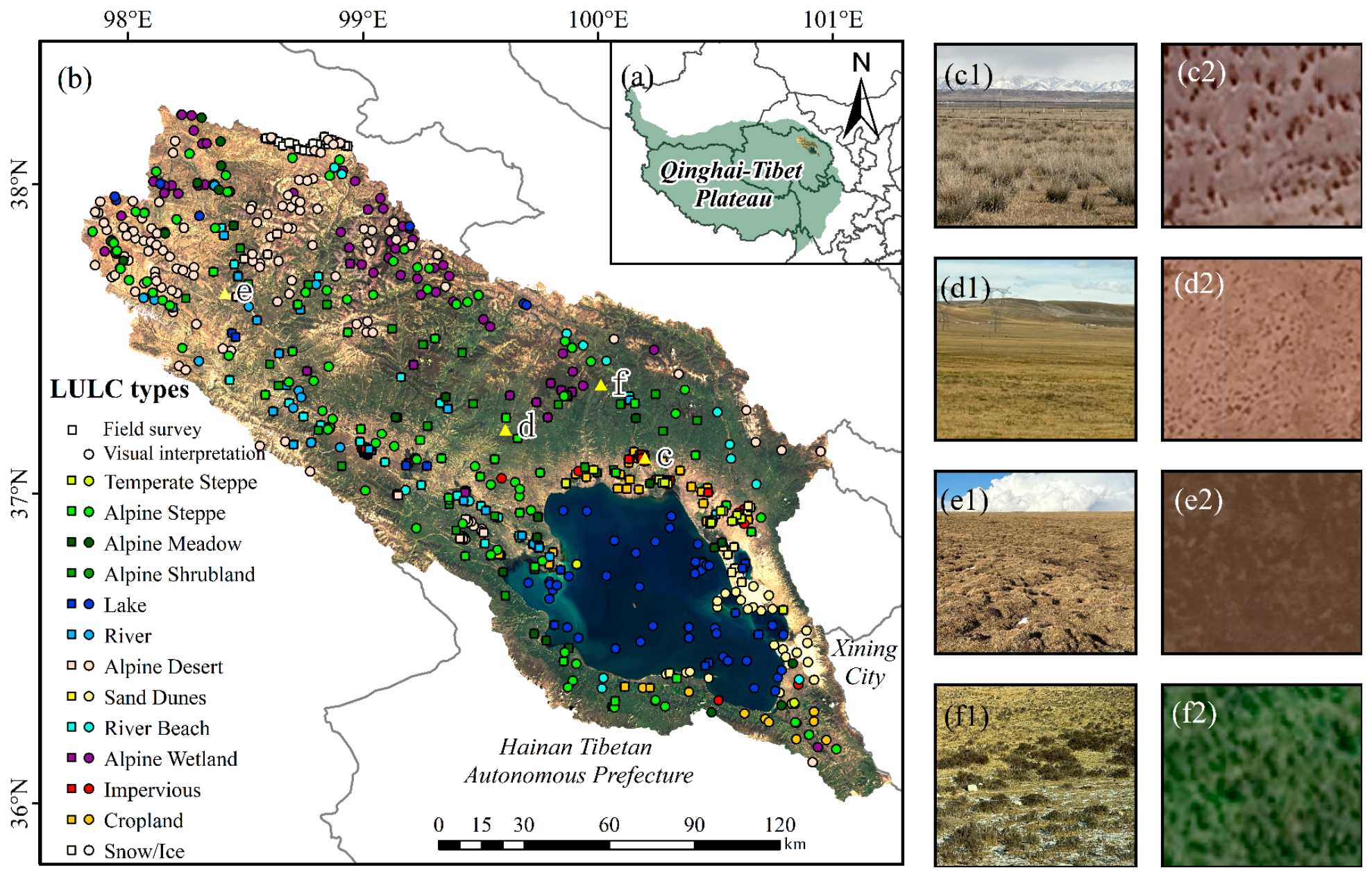
The QLB (36°15′–38°20′N, 97°50′–101°20′E), covering an area of 29,661 km², is located in the northeastern QTP within an ecological transition zone (Figure 1), with elevations ranging from 3194 to 5174 m [27]. It experiences a plateau continental climate characterized by intense diurnal temperature variations, mean annual temperatures of −1.5 to 1.5 °C, and concentrated summer precipitation (252–514 mm annually) that is far exceeded by extreme evaporation rates (1300–2000 mm) [28]. The Qinghai Lake surface was at 3197.52 m in 2025, with increasing water levels and area [29]. This unique topo-climatic environment fosters a highly heterogeneous landscape, yielding a complex mosaic of temperate steppes, alpine steppes, and alpine meadows.

Guided by prior knowledge accumulated through our long-term work in the QLB, we conducted a field survey in October 2024. To minimize spatial sampling bias, we adopted a strategy combining four-wheel-drive vehicles, unmanned aerial vehicles (UAVs), and on-foot surveys. Specifically, vehicles were utilized to penetrate mountainous regions as deeply as the terrain permitted, while for remote and complex areas that remained inaccessible by vehicles, we either deployed UAVs or proceeded on foot to complete the data collection. Through this approach, a total of 297 sample points were collected, covering all known LULC types within the QLB. To expand the dataset while mitigating spatial autocorrelation and preventing localized sample clustering, 7227 sample points were obtained through a block-based visual interpretation strategy using JiLin-1 imagery (0.5 m), multitemporal Sentinel-2 true-color composites, and high-resolution Google Earth imagery. These two approaches yielded 7524 sample points (Figure 1), which were carefully selected to ensure sufficient data for rare classes such as alpine shrublands, river beaches, lakes, and urban land, preventing the classifier from biasing toward dominant categories. In addition, the proportion of sample points across different altitude ranges is broadly consistent with the actual area proportions (

Table 1. Elevation-stratified distribution of the samples relative to the basin area.

Elevation Range (m)	Basin Area (km2)	Basin Area Proportion (%)	Sample Size	Sample Size Proportion (%)
[3200, 3400)	9265.52	30.98	2837	37.71
[3400, 3600)	3551.89	11.87	772	10.26
[3600, 3800)	3677.44	12.29	741	9.85
[3800, 4000)	4057.40	13.56	885	11.76
[4000, 4200)	4320.88	14.45	873	11.60
[4200, 4400)	3302.61	11.04	728	9.68
[4400, 4600)	1394.90	4.66	604	8.03
[4600, 4800)	294.24	0.98	58	0.77
[4800, 5000)	41.23	0.14	21	0.28
[5000, 5200]	6.36	0.02	5	0.07

), which improves the coverage of major elevation zones, reduces severe elevation under-representation, and prevents elevation bias to a certain degree. Such a scheme is well-suited to assembling a representative training set for the classifier, but it does not satisfy the conditions of probability sampling required for design-based inference. The accuracy figures derived from these samples are therefore treated throughout this study as apparent accuracies, which characterize agreement over the labeled reference data and are not generalized as unbiased estimates for the unsampled population (see Section 3.3 and Section 5.2).

2.2. Data

2.2.1. Satellite Data

Sentinel-1 provides C-band (5.405 GHz) synthetic aperture radar (SAR) backscatter data. We used 2024 Sentinel-1 GRD imagery (COPERNICUS/S1_GRD) at a 10-m resolution for winter (1 February to 31 March), spring (1 April to 31 May), summer (1 July to 31 August), and autumn (1 October to 30 November), provided by the Google Earth Engine (GEE) platform (https://code.earthengine.google.com, accessed on 25 April 2025). The pre-processing steps applied include radiometric calibration, range–Doppler terrain correction, and geo-registration, ensuring spatial consistency with the Sentinel-2 data. For each season, we generated median composites from descending-orbit interferometric wide (IW)-mode effective images in VV- and VH-polarizations and extracted the backscatter coefficient (σ⁰) to produce seasonally representative radar layers.

2024 Sentinel-2 Level-2A surface reflectance data (COPERNICUS/S2_SR_HARMONIZED) and the associated pixel-level cloud-probability product (COPERNICUS/S2_CLOUD_PROBABILITY) for winter, spring, summer, and autumn, obtained from the GEE platform, were used to characterize land-cover spectral properties. For each season, all available images covering the study area were filtered and masked using a 20% cloud probability threshold (probability ≤ 20%). We then applied a median composite to the cloud-filtered images using GEE’s time series functions to reduce noise from clouds, shadows, and outliers. Missing pixels generated by masking were filled using a local moving-window mean (radius of 2 pixels, three iterations). Sentinel-2 bands with a 20-m resolution were resampled to 10 m using bilinear interpolation, whereas 60-m bands were discarded.

2.2.2. Topographic Data

We used the Copernicus Global Digital Elevation Model (GLO-30), which provides a vertical accuracy better than 4 m and a horizontal accuracy better than 6 m, making it suitable for regional-scale terrain analysis [30]. The GLO-30 dataset (COPERNICUS/DEM/GLO30) was retrieved from GEE, resampled to 10 m using bilinear interpolation, and reprojected to ensure spatial consistency with the Sentinel imagery during analysis.

2.2.3. Auxiliary Data

Three widely used, high-resolution LULC datasets were compared with the QLBLC-10 dataset. FROM-GLC10 is a 10-m global product developed on the basis of Sentinel-2 imagery acquired in 2017, utilizing a classification scheme based on IGBP, GLC2000, and GLOBCover systems [5,8]. Similarly, GLC-FCS10 offers global coverage and was generated from time-series Sentinel-1/2 data for 2023 with a 10 m spatial resolution, referencing the classification systems of GWL_FCS30D and GLC_FCS30D [9]. On a regional scale, TPLCD was produced from Landsat imagery from 1990 to 2023 with a 30 m spatial resolution for the Tibetan Plateau, referencing the IGBP classification system [12]. These datasets were selected as representative LULC datasets with similar spatial resolutions, allowing for a robust and objective comparison with the QLBLC-10 obtained in this study.

3. Methods

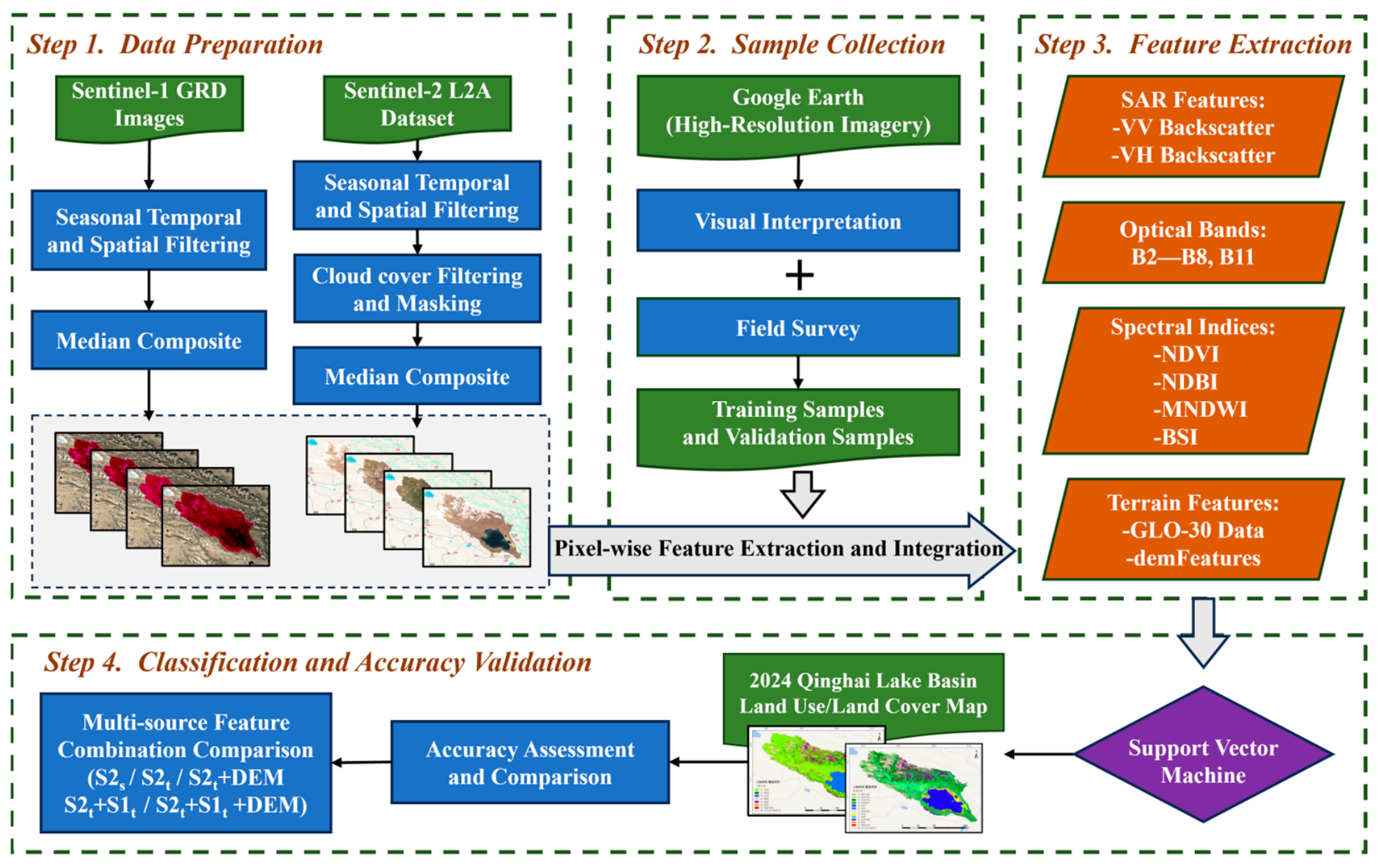
The workflow for this study is shown in Figure 2. This section presents the procedures for sample collection, feature construction, LULC classification, and accuracy assessment.

To assess how multitemporal optical data, radar observations, and terrain features contribute to classification, an ablation study was designed, with each scheme using a different input dataset (

Table 2. Eight schemes involved in the ablation experiments.

Scheme	Input Data Features
S2s	Summer median composite (S2 bands: 2–8, 11, +NDVI, NDBI, MNDWI, BSI)
S2t	Seasonal median composite (S2 bands: 2–8, 11, +NDVI, NDBI, MNDWI, BSI)
S2t + DEM	Seasonal median composite (S2 bands: 2–8, 11, +NDVI, NDBI, MNDWI, BSI) + DEM
S1t	Seasonal median composite (S1 polarizations: VV, VH)
S1t + DEM	Seasonal median composite (S1 polarizations: VV, VH) + DEM
S2s + S1s	Summer median composite (S2 bands: 2–8, 11, +NDVI, NDBI, MNDWI, BSI + S1 polarizations: VV, VH)
S2t + S1t	Seasonal median composite (S2 bands: 2–8, 11, +NDVI, NDBI, MNDWI, BSI + S1 polarizations: VV, VH)
S2t + S1t + DEM (QLBLC-10)	Seasonal median composite (S2 bands: 2–8, 11, +NDVI, NDBI, MNDWI, BSI + S1 polarizations: VV, VH) + DEM

). S2_s includes only summer Sentinel-2 bands and spectral indices, whereas S2_t incorporates multiseason Sentinel-2 bands and indices. S2_t + DEM is an intermediate scheme that adds elevation and elevation-zone variables derived from the DEM to the multiseason Sentinel-2 features. To isolate the independent contribution of radar, two schemes were included. S1_t uses multiseason Sentinel-1 VV and VH backscatter alone, and S1_t + DEM combines these multiseason radar features with the DEM-derived terrain variables. To separate the effect of multitemporal information from that of multisource fusion, a single-season fusion scheme (S2_s + S1_s) was also constructed from summer Sentinel-2 and summer Sentinel-1 features only. S2_t + S1_t then combines the full multiseason Sentinel-1 and Sentinel-2 features, and S2_t + S1_t + DEM further adds elevation and DEM-derived variables to constrain the spatial ranges of specific land cover types.

3.1. Construction of the Classification System

The widely referenced IGBP scheme fails to adequately represent the complexity and specificity of the LULC in alpine ecosystems. Therefore, in this study, the QLBLC-10 classification system (

Table 3. LULC classification system of the QLBLC-10.

Level-1 Classification		Level-2 Classification		Description
Code	Type	Code	Type
10	Grassland	11	Temperate Steppe	A grassland ecosystem distributed in temperate regions under a semiarid climate, dominated by herbaceous plants (most commonly Achnatherum splendens).
		12	Alpine Steppe	A high-altitude grassland ecosystem in cold, dry mountainous zones, dominated by cold- and drought-tolerant herbaceous plants.
		13	Alpine Meadow	A grassland ecosystem at high elevations, in cold and relatively moist climatic conditions, with dense vegetation dominated by perennial herbaceous plants.
20	Shrubland	20	Alpine Shrubland	A shrubland ecosystem in high–cold environments, with cold-tolerant shrubs as the dominant vegetation.
30	Water	31	Lake	A larger body of standing water formed in a land depression, long-lasting, and lacking an obvious connection to the sea.
		32	River	A body of surface water flowing in a defined direction, typically with a source, a channel, and an outlet.
40	Barren	41	Alpine Desert	A high-elevation arid ecosystem in cold mountainous zones with extreme dryness, sparse vegetation (often <20% cover), poor soils, and fragile ecological conditions.
		42	Sand Dunes	Landforms formed by the accumulation of sand grains, shaped by wind and other processes.
		43	River Beach	Low-lying, flat terrain along a riverbank, typically formed by fluvial (river-sediment) deposition.
50	Wetland	50	Alpine Wetland	A broad area at high altitude, frequently or permanently inundated with water (fresh, brackish, or saline) and vegetated with herbaceous or woody plants; a transitional zone between land and open water.
60	Cropland	60	Cropland	Lands suitable and used for agricultural production; typically located in valley bottoms or lake-shore zones with modest acreage of farmland.
70	Impervious	70	Impervious	Lands covered by buildings and other man-made structures.
80	Snow/Ice	80	Snow/Ice	Lands under snow or ice cover for most or all of the year.

) was designed based on the Current Land Use Classification of China (GB/T 21010–2017), with reference to the IGBP and existing LULC datasets [31,32,33]. We adapted the system to the ecological characteristics of the QLB by simplifying the original IGBP categories and reducing the emphasis on forest and savanna types. Based on elevation, moisture availability, and dominant species, grasslands were further subdivided into three ecologically meaningful subclasses [34]. According to field surveys, temperate steppes occur at lower lake-side elevations and are dominated by Achnatherum splendens and Stipa caucasica. Moving to colder and drier zones, alpine steppes emerge with Artemisia frigida and Stipa purpurea. Alpine meadows occur at even higher elevations with greater moisture availability and are dominated by Kobresia myosuroides.

3.2. Classification Method

3.2.1. Feature Space Construction

Constructing an effective feature dataset is essential for LULC mapping. To enhance class separability, eight representative bands, i.e., B2 (490 nm), B3 (560 nm), B4 (665 nm), B5 (705 nm), B6 (740 nm), B7 (783 nm), B8 (842 nm), and B11 (1610 nm), were extracted from the seasonal Sentinel-2 images as feature inputs for SVM. Numerous studies have demonstrated that incorporating spectral indices improves LULC classification performance [35]. Another four widely used spectral indices were introduced to SVM to optimize classification accuracy: the normalized difference vegetation index (NDVI), the normalized difference built-up index (NDBI), the modified normalized difference water index (MNDWI), and the bare soil index (BSI). Their formulas are as follows:

$$\mathrm{N}\mathrm{D}\mathrm{V}\mathrm{I}={\displaystyle \frac{\mathrm{B}8-\mathrm{B}4}{\mathrm{B}8+\mathrm{B}4}}$$

(1)

$$\mathrm{N}\mathrm{D}\mathrm{B}\mathrm{I}={\displaystyle \frac{\mathrm{B}11-\mathrm{B}8}{\mathrm{B}11+\mathrm{B}8}}$$

(2)

$$\mathrm{M}\mathrm{N}\mathrm{D}\mathrm{W}\mathrm{I}={\displaystyle \frac{\mathrm{B}3-\mathrm{B}11}{\mathrm{B}3+\mathrm{B}11}}$$

(3)

$$\mathrm{B}\mathrm{S}\mathrm{I}={\displaystyle \frac{\left(\mathrm{B}11+\mathrm{B}4\right)-(\mathrm{B}8+\mathrm{B}2)}{\left(\mathrm{B}11+\mathrm{B}4\right)+(\mathrm{B}8+\mathrm{B}2)}}$$

(4)

In addition, the seasonal time series features of Sentinel-1 VV and VH backscatter were extracted to incorporate multitemporal radar information. With respect to terrain characteristics, three elevation-based auxiliary variables (below_3700 m, above_3800 m, and above_3200 m) were derived from the GLO-30 DEM data. These elevation intervals were determined through quantitative analysis of the class-wise elevation distributions of samples for elevation-sensitive LULC.

By integrating the eight primary spectral bands, four spectral indices, VV/VH radar backscatter features, and DEM-derived variables, a total of 60 feature layers were constructed for model training (

Table 4. The feature sets used in this study.

Feature Type		Feature Name
Spectral Bands	B2 (Blue)	B2_spring, B2_summer, B2_autumn, B2_winter
	B3 (Green)	B3_spring, B3_summer, B3_autumn, B3_winter
	B4 (Red)	B4_spring, B4_summer, B4_autumn, B4_winter
	B5 (VNIR)	B5_spring, B5_summer, B5_autumn, B5_winter
	B6 (VNIR)	B6_spring, B6_summer, B6_autumn, B6_winter
	B7 (VNIR)	B7_spring, B7_summer, B7_autumn, B7_winter
	B8 (NIR)	B8_spring, B8_summer, B8_autumn, B8_winter
	B11 (SWIR)	B11_spring, B11_summer, B11_autumn, B11_winter
Spectral Index	NDVI	NDVI_spring, NDVI_summer, NDVI_autumn, NDVI_winter
	NDBI	NDBI_spring, NDBI_summer, NDBI_autumn, NDBI_winter
	MNDWI	MNDWI_spring, MNDWI_summer, MNDWI_autumn, MNDWI_winter
	BSI	BSI_spring, BSI_summer, BSI_autumn, BSI_winter
Polarization	VV	VV_spring, VV_summer, VV_autumn, VV_winter
	VH	VH_spring, VH_summer, VH_autumn, VH_winter
Terrain Data	DEM	Elevation
	demFeatures	Below_3700 m
		Above_3800 m
		Above_3200 m

).

3.2.2. SVM-Based Classification

The SVM constructs an n-dimensional hyperplane that separates the dataset into distinct classes [36]. In alpine areas, field sample collection is often constrained by complex terrain and harsh climatic conditions, resulting in relatively small and spatially heterogeneous training datasets. Under such circumstances, SVM has demonstrated strong generalization capability to effectively balance empirical error and model complexity [26]. Following recommendations by Mountrakis et al. and Duro et al. [37,38], the radial basis function (RBF) kernel—commonly used in remote-sensing image analysis—was adopted. The RBF kernel maps input features into a higher-dimensional space, enabling the model to capture nonlinear boundaries among land cover types, which are common in heterogeneous alpine landscapes where spectral and structural characteristics overlap. Prior to training, all input features were normalized to [0, 1] to prevent variables with larger ranges from dominating the kernel distance. The SVM hyperparameters (cost C and kernel width γ) were tuned by grid search with 5-fold cross-validation over C ∈ {0.1, 1, 10} and γ ∈ {0.001, 0.01, 1/60, 0.1, 1}. The optimal parameters were C = 1 and γ = 1/60.

The samples were randomly partitioned within each class into training and validation subsets, with 70% for classifier training and the remaining 30% reserved for accuracy assessment (

Table 5. Number of training and validation samples.

Level-1 Classification		Level-2 Classification		Number
Code	Type	Code	Type	Training Pixels	Validation Pixels
10	Grassland	11	Temperate Steppe	454	144
		12	Alpine Steppe	413	136
		13	Alpine Meadow	316	93
20	Shrubland	20	Alpine Shrubland	383	122
30	Water	31	Lake	308	101
		32	River	643	176
40	Barren	41	Alpine Desert	778	231
		42	Sand Dunes	579	188
		43	River Beach	334	104
50	Wetland	50	Alpine Wetland	350	114
60	Cropland	60	Cropland	447	124
70	Impervious	70	Impervious	313	90
80	Snow/Ice	80	Snow/Ice	449	134

).

3.2.3. Post-Classification Processing

Pixel-based classifications typically exhibit salt-and-pepper noise [39]. To improve spatial consistency and reduce classification noise, isolated clusters of fewer than 20 contiguous pixels were removed and set to NoData. A 9 × 9 majority filter was then applied only to these removed pixels, reassigning each of them to the majority class within its moving window [39,40]. To justify the selection of the 20-pixel spatial threshold, a threshold sensitivity analysis was conducted by testing alternative cluster sizes of 10 and 30 pixels (Section 4.2.1).

3.3. Assessment of Accuracy

A confusion matrix (CM) was used to evaluate the classification accuracy [41,42], from which the sample-based OA, kappa coefficient, producer accuracy (PA), and user accuracy (UA) were derived. While OA denotes the overall proportion of correctly classified samples, PA and UA specifically reflect omission and commission errors, respectively, and the kappa coefficient measures classification agreement beyond random chance [43]. It should be noted that the reference samples used here were obtained through a sample-based design. Consequently, all of the metrics defined above are reported throughout this study as apparent accuracies.

The formulas used in this study are as follows:

$$OA={\displaystyle \frac{{\displaystyle {\sum }_{i=1}^n}{X}_{ii}}{N}}\times 100\%$$

(5)

$$Kappa={\displaystyle \frac{N\times {\displaystyle {\sum }_{i=1}^n}{X}_{ii}-{\displaystyle {\sum }_{i=1}^n}(G_i\times C_i)}{N}}$$

(6)

$$PA={\displaystyle \frac{X_{ii}}{X_{+i}}}\times 100\%$$

(7)

$$UA={\displaystyle \frac{X_{ii}}{X_{i+}}}\times 100\%$$

(8)

where $N$ is the total number of validation samples, $n$ is the number of classes in the CM, $X_{ii}$ is the number of correctly classified samples (diagonal elements), and $X_{+i}$ and $X_{i+}$ represent the marginal totals for column $i$ and row $i$, respectively.

To examine how strongly the proportions of mapped class areas influence the reported accuracy, we implemented the area-weighted accuracy assessment proposed by Olofsson et al. [44]. The area-weighted estimators applied in Section 5.2 rescale the confusion matrix by the mapped area of each class; they correct only for class-area proportions and not for the spatial selection mechanism of the samples, so the area-weighted figures are likewise apparent accuracies.

$${OA}_w={\displaystyle \sum _{i=1}^n}{W}_i\times {UA}_i\times 100\%$$

(9)

where $W_i$ is the area proportion of class $i$ mapped in the classification result, and ${UA}_i$ is the sample-based UA.

Furthermore, we calculated the ${PA}_w$. This is derived from the proportions within the area-weighted confusion matrix ($p_{ij}$):

$${PA}_w={\displaystyle \frac{p_{jj}}{{\widehat{p}}_{+j}}}$$

(10)

where $p_{jj}$ is the estimated area proportion correctly classified for class $j$ (calculated as $W_j\times {UA}_j$), and ${\widehat{p}}_{+j}$ is the estimated true population area proportion of class $j$, calculated by summing the area-weighted proportions across all map classes.

In addition, the F1-score was calculated to provide a balanced evaluation of classification performance for each class [45]. The F1-score is defined as the harmonic mean of precision (UA) and recall (PA):

$${F1}_i={\displaystyle \frac{2\times ({PA}_i\times {UA}_i)}{{PA}_i+{UA}_i}}$$

(11)

To better characterize classification performance for the rare essential classes, the macro-averaged F1-score was computed:

$$\mathrm{macro}\text{-}\mathrm{averaged} F1={\displaystyle \frac{{\displaystyle {\sum }_{i=1}^n}{F}_i}{N}}$$

(12)

The paired McNemar test with continuity correction was applied to the matched validation set, with a significance level of α = 0.05 and Bonferroni-correction applied for multiple comparisons [46].

To further assess the robustness and advantages of the proposed classification, QLBLC-10-L1 was compared with FROM-GLC10, GLC-FCS10, and TPLCD. All maps were harmonized to a unified classification scheme corresponding to QLBLC-10-L1 and clipped to the study area (

Table 6. Classification system mapping relationship.

FROM-GLC10	GLC-FCS10	TPLCD	Unified Category
Grassland, Tundra	Grassland, lichens and mosses, sparse vegetation	Alpine steppe, Alpine meadow	Grassland
Shrubland, Forest	Closed evergreen needle-leaved forest, closed evergreen broadleaved forest, closed deciduous needle-leaved forest, closed deciduous broadleaved forest, open deciduous needle-leaved forest, evergreen shrubland, deciduous shrubland	Forest, Shrub	Shrubland
Water	Lake/river flat, water body	Water bodies	Water
Barren	Saline, bare areas	Bare land	Barren
Wetland	Marsh	Wetlands	Wetland
Cropland	Herbaceous rainfed cropland, irrigated cropland	Cropland	Cropland
Impervious	Urban impervious surfaces, rural impervious surfaces	Impervious surfaces	Impervious
Snow/Ice	Permanent ice and snow	Snow/Ice	Snow/Ice

).

4. Results

4.1. Ablation Study Results

The apparent OA and kappa of all eight schemes are summarized in

Table 7. Comparison of the PAs/UAs under eight classification schemes.

LULC Type	S2s		S2t		S2t + DEM		S1t		S1t + DEM		S2s + S1s		S2t + S1t		S2t + S1t + DEM
	PA (%)	UA (%)	PA (%)	UA (%)	PA (%)	UA (%)	PA (%)	UA (%)	PA (%)	UA (%)	PA (%)	UA (%)	PA (%)	UA (%)	PA (%)	UA (%)
Temperate Steppe	96.90	89.29	96.72	91.47	96.24	88.28	85.82	64.25	96.06	89.71	96.48	86.71	97.04	94.93	94.63	97.92
Alpine Steppe	51.72	45.80	73.13	54.44	17.97	17.97	41.38	36.09	57.60	55.81	60.28	62.50	74.14	62.32	68.84	69.85
Alpine Meadow	10.87	40.00	36.89	63.33	36.00	67.92	43.30	57.53	55.21	58.89	42.35	45.00	63.55	72.34	68.48	67.74
Alpine Shrubland	67.21	64.57	81.36	81.36	93.52	46.76	28.23	49.30	61.06	60.53	64.35	74.00	85.00	77.86	77.24	77.87
Lake	91.49	100.00	98.84	100.00	97.92	68.61	67.86	81.43	94.29	93.40	94.44	100.00	98.57	100.00	100.00	97.03
River	92.61	94.95	95.67	98.51	63.92	97.12	88.67	80.72	91.16	91.67	95.21	97.55	99.45	95.79	96.57	96.02
Alpine Desert	66.12	65.70	90.53	97.35	94.50	90.75	91.95	90.04	95.43	95.00	91.59	85.54	95.89	99.53	97.40	97.40
Sand Dunes	83.82	71.43	97.78	95.65	96.63	97.18	78.41	81.18	83.43	93.21	99.35	96.23	99.48	100.00	100.00	97.87
River Beach	64.36	64.36	83.33	86.42	82.14	85.19	56.64	57.66	75.76	79.79	70.75	65.79	83.33	85.00	86.67	87.50
Alpine Wetland	96.30	84.55	93.40	100.00	22.12	85.19	78.38	78.38	86.73	83.33	97.39	93.33	85.57	96.51	93.75	92.11
Cropland	91.22	97.83	99.21	97.67	98.37	95.28	97.04	89.73	97.60	94.57	96.83	96.06	97.04	100.00	92.97	95.97
Impervious	66.29	54.63	94.79	79.82	90.32	83.17	70.89	68.29	93.55	87.00	65.69	78.82	89.53	92.77	95.45	93.33
Snow/Ice	100.00	100.00	100.00	100.00	100.00	99.29	80.31	81.60	100.00	100.00	100.00	100.00	100.00	100.00	100.00	100.00
OA (%)	77.07		88.95		78.12		73.31		84.93		84.84		91.21		91.24
Kappa	0.75		0.88		0.76		0.71		0.84		0.83		0.90		0.90

. These ablation experiments can isolate the specific contributions of distinct features to the classification process. The apparent OA increased from 77.07% for the S2_s-derived map to 91.24% for the S2_t + S1_t + DEM-derived map, and the kappa coefficient increased from 0.75 to 0.90. S1_t produced the lowest accuracy, with an OA of 73.31%, but combining it with DEM (S1_t + DEM) raised the OA to 84.93%. S2_s + S1_s reached an OA of 84.84%, well below the 91.21% of S2_t + S1_t, indicating that the seasonal, multitemporal features account for a substantial part of the accuracy gain.

The McNemar test results (

Table 8. The McNemar test results for the statistical significance of accuracy differences among different feature combinations.

Comparison (Scheme A vs. Scheme B)	b (A Correct, B Wrong)	c (A Wrong, B Correct)	χ2	p
S2s vs. S2t	34	316	225.60	5.42 × 10−51
S2t vs. S2t + S1t	30	79	21.14	4.28 × 10−6
S2t + S1t vs. S2t + S1t + DEM	65	41	4.99	0.025
S2s + S1s vs. S2t + S1t	34	167	86.69	1.27 × 10−20

Note: A Bonferroni-corrected significance level of α = 0.0125 (0.05/4) was applied to control the family-wise error rate across multiple comparisons.

) confirm that the accuracy improvement resulting from the integration of Sentinel-1 SAR data was statistically significant (p < 0.001).

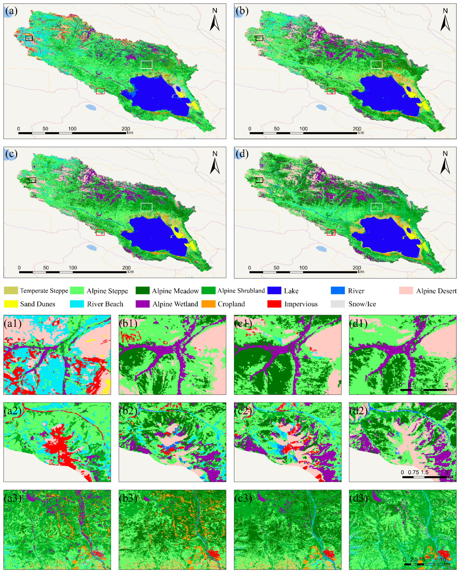
Compared with the single-season optical data (S2_s) derived map (Figure 3a), incorporating multiseason data (S2_t) effectively separated grasslands with distinct phenologies, such as alpine steppe, alpine meadow, and alpine shrubland (Figure 3(b3)). Furthermore, adding radar data (S2_t + S1_t) significantly improved the discrimination among spectrally similar classes, including sand dunes, alpine deserts, and impervious surfaces (Figure 3c). Finally, the integration of terrain features (S2_t + S1_t + DEM) reduced the spatial confusion between high-elevation alpine deserts and lower-elevation impervious or river beach classes (Figure 3(d2)).

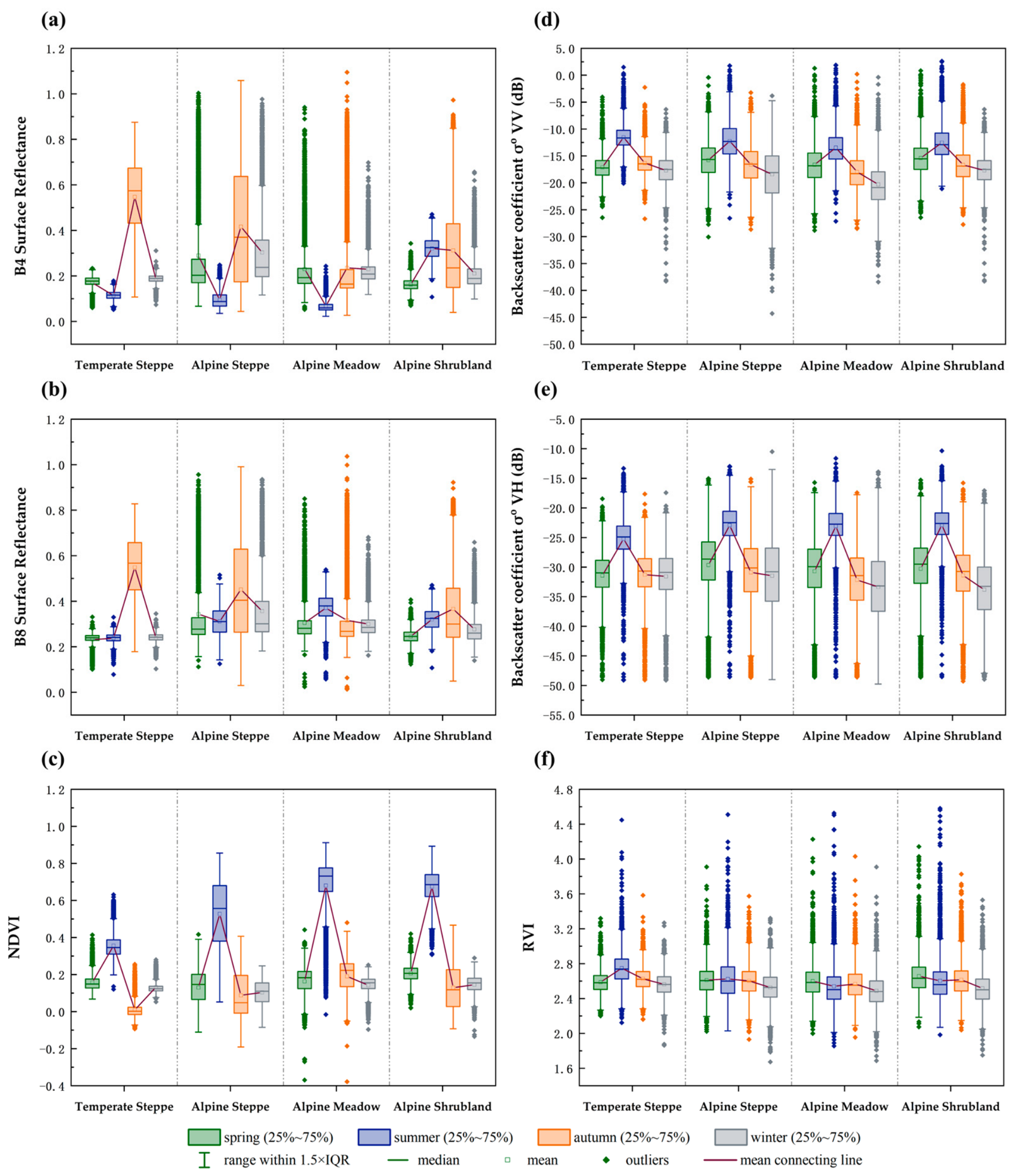
The integration of multiseason Sentinel-1 radar backscatter with multitemporal Sentinel-2 optical data enhanced mapping performance. The OA improved from 88.95% to 91.21%, and the kappa coefficient increased from 0.88 to 0.90 (Table 7). Notably, the UA for alpine meadows substantially increased from 36.89% to 63.55%. To understand this accuracy gain, we focused on true alpine meadow pixels initially misclassified into other vegetation types by optical-only data, but successfully corrected after incorporating Sentinel-1 backscatter. A bootstrap analysis (5000 pixels/class, 2000 iterations) revealed that despite highly variable optical patterns, these pixels displayed consistent seasonal trajectories in VV and VH backscatter (Figure 4). This demonstrates that the SVM classifier effectively captured discriminative radar signatures that are not evident in optical data.

By adding DEM to multiseason optical data alone, the OA decreased from 88.95% (S2_t) to 78.12% (S2_t + DEM). This decline was concentrated in alpine steppe, whose PA and UA both fell to 17.97%, and in alpine wetland, whose PA dropped from 93.40% to 22.12%, while river and lake became harder to separate (Table 7). In contrast, adding the DEM to Sentinel-1 data alone raised the OA from 73.31% (S1_t) to 84.93% (S1_t + DEM), and adding it to the combined optical–radar features produced the highest accuracy of all schemes (S2_t + S1_t + DEM, 91.24%); under this scheme, classes with similar elevations remained well-classified. The mechanism underlying this conditional behavior is examined in Section 5.1.2.

4.2. Accuracy Assessment of QLBLC-10

4.2.1. Classification Results

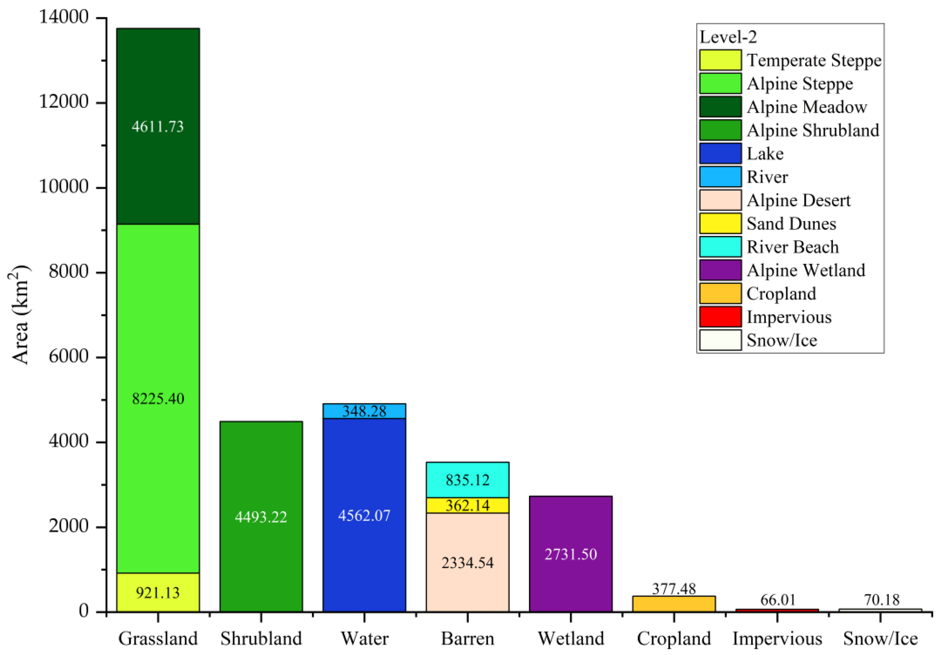
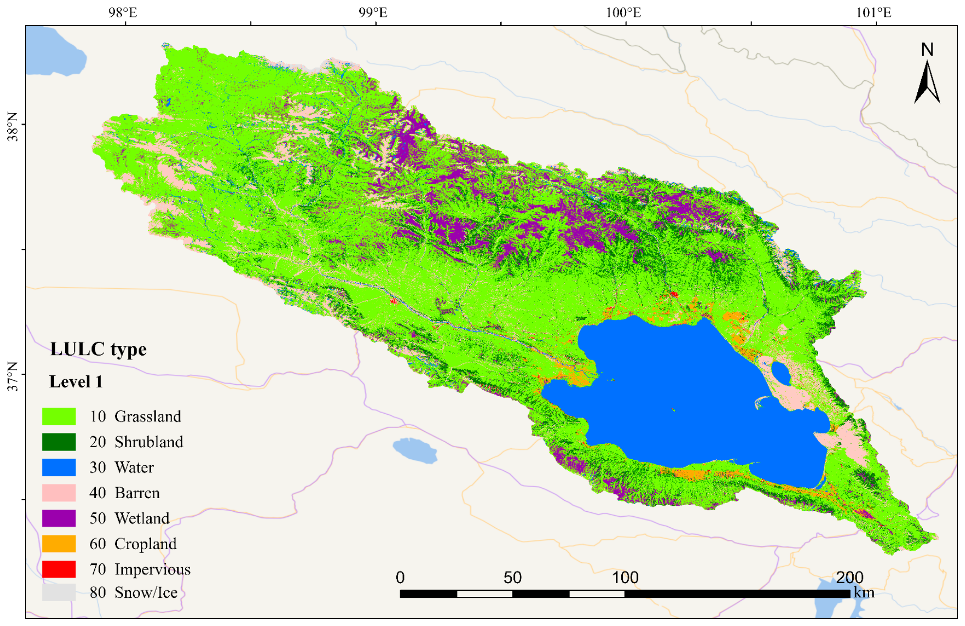
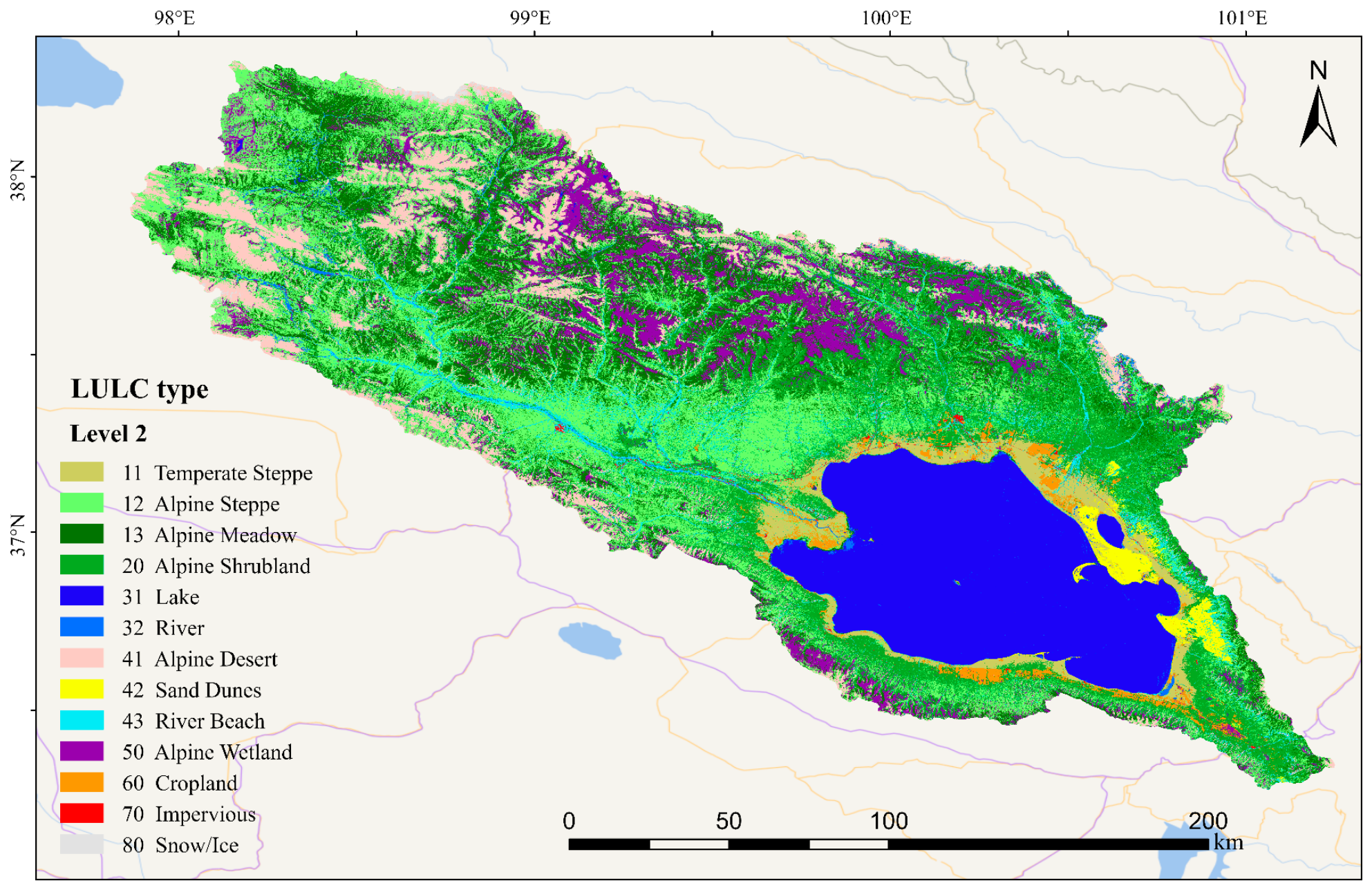
Figure 5 and Figure 6 present the area and spatial distribution of QLBLC-10-L1 and QLBLC-10-L2 LULC types based on the best scheme (S2_t + S1_t + DEM), respectively.

In QLBLC-10-L1, the LULC pattern of the QLB is dominated by grassland, which accounts for 46.05% of the total area, whereas water, shrubland, barren land, and wetlands constitute the remaining major components (Figure 7), respectively accounting for 16.44%, 15.04%, 11.82%, and 9.15% of the total area.

It is worth noting that the impact of post-classification processing on the classification results of QLBLC-10 was also evaluated. As demonstrated in Tables S1 and S2, the influence was small. In addition, the classification results were not sensitive to patch size when patches were set to 10, 20, and 30 (Table S3), and the 20-pixel setting was retained as a balance between noise suppression and the preservation of small, genuine patches.

4.2.2. Classification Accuracy

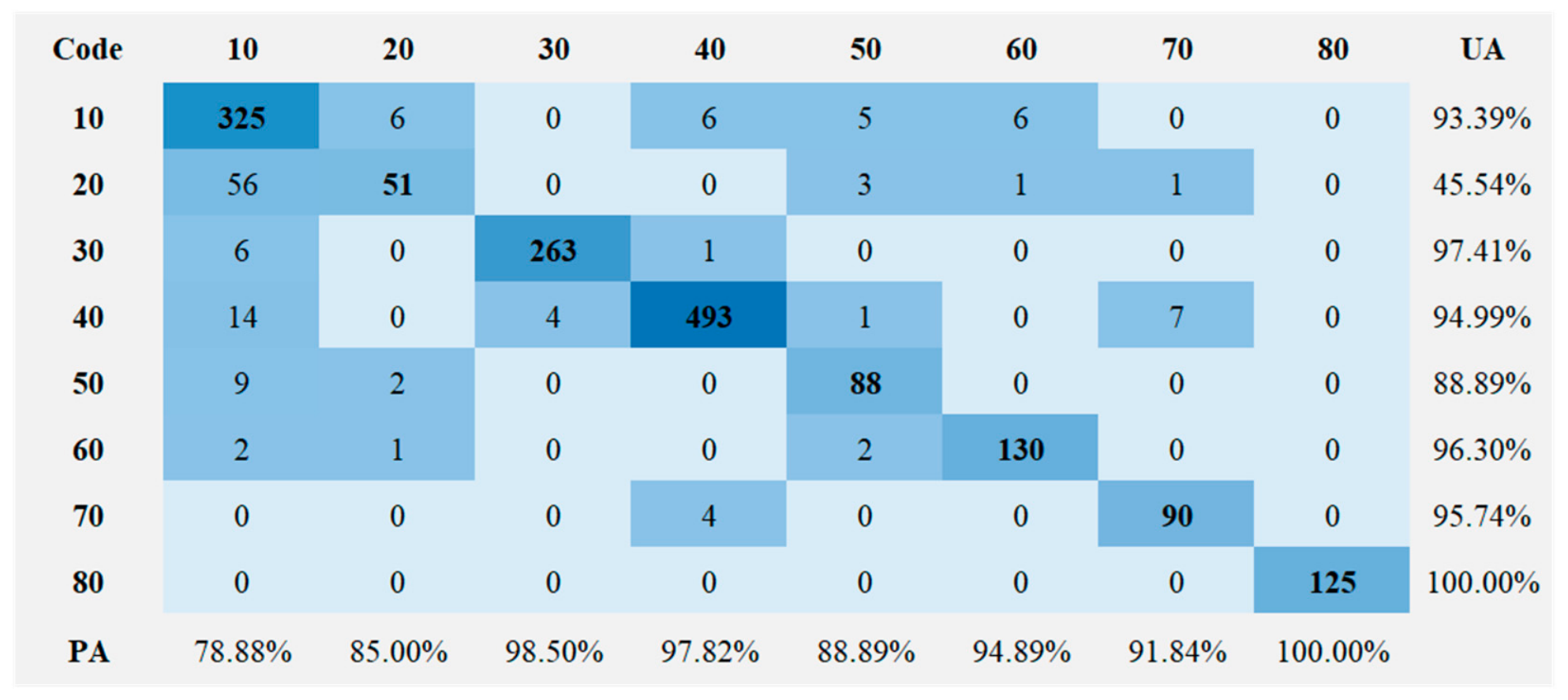
The QLBLC-10 product demonstrated robust classification efficacy at both hierarchical levels. For QLBLC-10-L1 (Figure 8), the apparent OA reached 91.95%, with a kappa coefficient of 0.90. Grassland, water, barren, cropland, impervious surfaces, and snow/ice classes all exceeded 93% in UA, with snow/ice achieving perfect accuracy (PA and UA of 100%). In contrast, shrubland showed a lower UA of 45.54%, with 56 validation samples misclassified as grassland.

To further characterize class-wise performance under potential class imbalance, we additionally computed per-class F1-scores and macro-averaged F1 (

Table 9. F1-scores and the macro-averaged F1 for the Level-1 and Level-2 LULC categories.

Level-1 Classification	F1i	Level-2 Classification	F1i
Grassland	0.8553	Temperate Steppe	0.9625
		Alpine Steppe	0.6934
		Alpine Meadow	0.6811
Shrubland	0.5930	Alpine Shrubland	0.7755
Water	0.9795	Lake	0.9849
		River	0.9630
Barren	0.9638	Alpine Desert	0.9740
		Sand Dunes	0.9892
		River Beach	0.8708
Wetland	0.8889	Alpine Wetland	0.9292
Cropland	0.9559	Cropland	0.9444
Impervious	0.9375	Impervious	0.9438
Snow/Ice	1.0000	Snow/Ice	1.0000
Macro avg F1	0.8967		0.9009

). The Level-1 macro-F1 reached 0.8967, while the shrubland F1-score was 0.5930. Given that the ecotone boundary between shrubland and grassland serves as a critical indicator of alpine ecosystem dynamics in the QLB, the substantial spectral and structural confusion between these two classes represents a specific limitation of the current dataset. Consequently, although the overall map accuracy remains robust, users should exercise caution when utilizing the shrubland category for fine-scale ecological monitoring or strict boundary delineations.

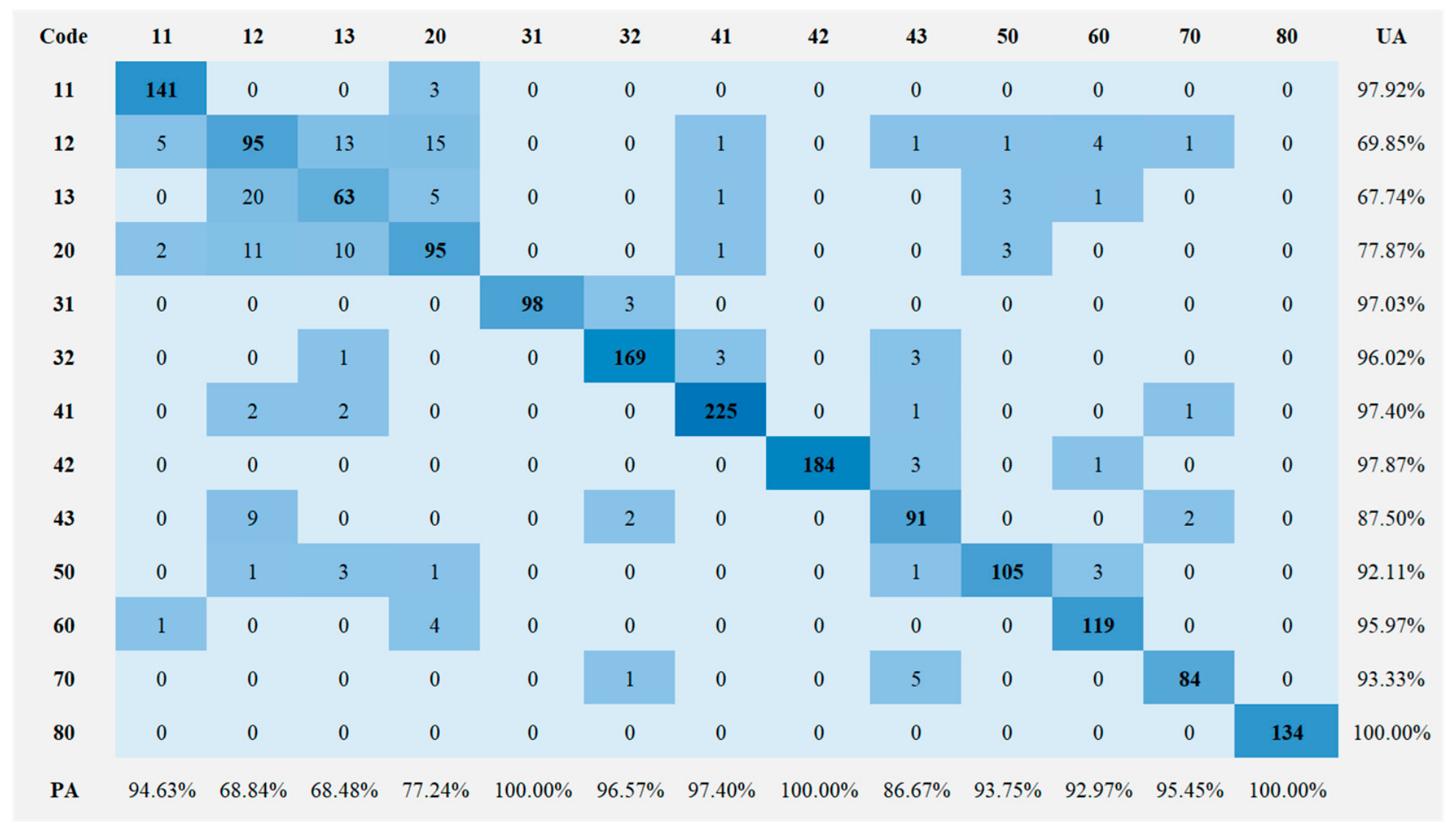
At QLBLC-10-L2, the apparent OA remained high at 91.24%, with a kappa coefficient of 0.90 (Figure 9) and an area-weighted OA_w of 81.50 ± 2.09% (95% confidence interval) (

Table 10. Area-weighted apparent accuracy metrics for the QLBLC-10-L2.

LULC Type	Wi	PA (%)	UA (%)	${\mathit{p}}_{\mathit{j}\mathit{j}}$	${\widehat{\mathit{p}}}_{+\mathit{j}}$	${\mathit{P}\mathit{A}}_{\mathit{w}}$ (%)
Temperate Steppe	0.0308	94.63	97.92	0.0301	0.0428	70.41
Alpine Steppe	0.2747	68.84	69.85	0.1919	0.2425	79.15
Alpine Meadow	0.1540	68.48	67.74	0.1043	0.1461	71.44
Alpine Shrubland	0.1501	77.24	77.87	0.1169	0.1617	72.26
Lake	0.1524	100.00	97.03	0.1479	0.1479	100.00
River	0.0116	96.57	96.02	0.0112	0.0163	68.71
Alpine Desert	0.0780	97.40	97.40	0.0759	0.0811	93.70
Sand Dunes	0.0121	100.00	97.87	0.0118	0.0118	100.00
River Beach	0.0279	86.67	87.50	0.0244	0.0281	86.92
Alpine Wetland	0.0912	93.75	92.11	0.0840	0.0947	88.73
Cropland	0.0126	92.97	95.97	0.0121	0.0243	49.79
Impervious	0.0022	95.45	93.33	0.0021	0.0050	41.56
Snow/Ice	0.0023	100.00	100.00	0.0023	0.0023	100.00
OAw (%)	81.50 ± 2.09

). The macro-F1 reached 0.9009 (Table 9). This consistency indicates that the classifier maintained stable performance even under a more detailed scheme. Most Level-2 classes—including temperate steppe, lake, river, alpine desert, sand dunes, alpine wetland, cropland, impervious, and snow/ice—achieved PA and UA values above 90%.

4.3. Comparison with Existing Products

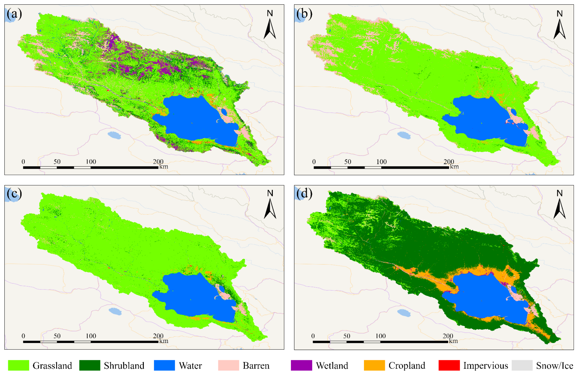
After harmonizing the classification schemes, we compared QLBLC-10-L1 with the three products both quantitatively (

Table 11. Accuracy comparison of QLBLC-10-L1 and three existing products based on the unified Level-1 classification system.

LULC Type	QLBLC-10		FROM-GLC10		GLC-FCS10		TPLCD
	PA (%)	UA (%)	PA (%)	UA (%)	PA (%)	UA (%)	PA (%)	UA (%)
Grassland	78.88	93.39	92.37	49.42	97.28	41.18	54.50	33.22
Shrubland	85.00	45.54	4.04	100.00	1.01	3.45	1.01	100.00
Water	98.50	97.41	62.41	98.84	80.29	93.62	72.63	92.56
Barren	97.82	94.99	82.21	70.77	38.73	89.15	54.19	74.44
Wetland	88.89	88.89	0.00	0.00	0.00	0.00	1.04	33.33
Cropland	94.89	96.30	79.47	94.49	98.68	100.00	94.70	43.07
Impervious	91.84	95.74	0.00	0.00	80.22	100.00	58.24	96.36
Snow/Ice	100.00	100.00	100.00	97.95	100.00	99.31	98.70	95.00
OA (%)	91.95		68.95		66.24		60.58
Kappa	0.90		0.61		0.59		0.50

) and visually (Figure 10). Evaluated on this common validation set, QLBLC-10-L1 achieved an OA of 91.95% and a kappa coefficient of 0.90, exceeding FROM-GLC10 (OA = 68.95%, Kappa = 0.61), GLC-FCS10 (OA = 66.24%, Kappa = 0.59), and TPLCD (OA = 60.58%, Kappa = 0.50). While the three datasets report high OAs at global or regional scales, they inevitably exhibit localized discrepancies when applied to highly heterogeneous areas like the QLB. Such performance variations do not negate their extensive large-scale utility; rather, they highlight the necessity of developing regionally tailored products—such as QLBLC-10—to accurately capture fine-grained alpine land-cover details.

At the class level (Table 11), the three products remained reliable for distinct categories. Snow/ice was captured almost perfectly by all of them (PA ≥ 98.70%, UA ≥ 95.00%), and water was retained with high reliability (UA = 98.84%, 93.62%, and 92.56% for FROM-GLC10, GLC-FCS10, and TPLCD, respectively), while FROM-GLC10 also performed acceptably for barren land (PA = 82.21%, UA = 70.77%). Their accuracy degraded sharply, however, for the heterogeneous classes that dominate the basin. All three products yielded high PA but low UA for grassland (UA = 49.42%, 41.18%, and 33.22%), which indicates that other cover types are frequently absorbed into the grassland class. FROM-GLC10 and GLC-FCS10 further retained forestland categories that are largely absent in the QLB. Shrubland was almost entirely omitted (PA = 4.04%, 1.01%, and 1.01%). Notably, the wetland was undetected by FROM-GLC10 and GLC-FCS10 and nearly so by TPLCD (PA = 1.04%). This omission is largely driven by nomenclature and definitional divergences among the classification systems. FROM-GLC10 relies on forest-centric definitions (e.g., “swamp forest” or “mangrove forest” requiring vegetation heights above 3 m). Because the native legends of these existing products were not designed to accommodate alpine ecological traits, they failed to capture the wetlands in this region. Furthermore, impervious surfaces were not captured by FROM-GLC10, whereas GLC-FCS10 and TPLCD recovered them more successfully (PA = 80.22% and 58.24%, respectively). TPLCD was the only external product whose native legend explicitly separates alpine steppe and alpine meadow, conceptually closer to the QLB landscape [12]; this design, however, does not translate into higher Level-1 accuracy, as TPLCD recorded the lowest OA among the three products, largely because it overestimates croplands and confuses them with wetlands (cropland UA = 43.07%), likely due to its direct use of DEM inputs [47]. In contrast, QLBLC-10-L1 maintained a balanced performance across all eight Level-1 classes (PA = 78.88–100%, UA = 45.54–100%), and in particular, recovered the shrubland, wetland, and impervious classes that the existing products struggled to delineate.

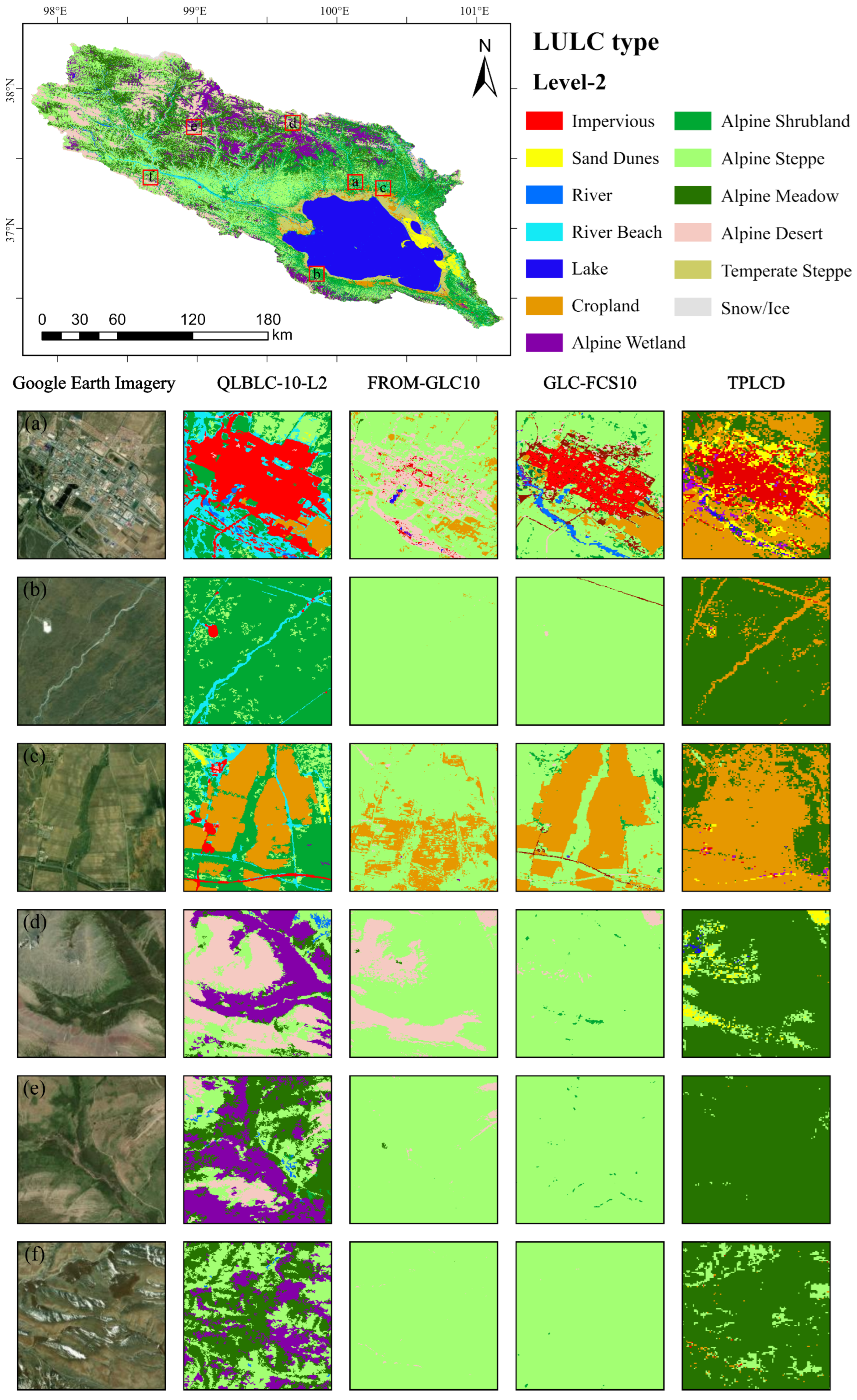
High-resolution Google Earth imagery was further compared with QLBLC-10-L2 and the three reference products across six representative areas in Figure 11. FROM-GLC10 and GLC-FCS10 provide robust and valuable references for broad land cover patterns, while QLBLC-10-L2 captures finer spatial details of impervious surfaces, rivers, and alpine steppes (Figure 11a–c). The spatial pattern of the alpine desert in QLBLC-10-L2 was broadly consistent with that in FROM-GLC10 (Figure 11d). QLBLC-10-L2 demonstrated improved separability between the alpine desert and adjacent alpine wetland, alpine steppe, and alpine meadow (Figure 11e). Despite these improvements, some fragmentation remained in the grassland and shrubland subclasses (Figure 11f).

Although deep learning–based LULC classification methods have advanced rapidly in recent years, their performance typically depends on large, well-labeled training data and substantial computational resources. In alpine regions such as the QLB, where climatic conditions are harsh and labeled samples are limited, these requirements are difficult to meet. Under such conditions, SVM remains a practical and effective alternative. Its generalization capability under small-sample conditions, together with the explicit integration of spectral, radar, and elevation features, facilitated the discrimination of spectrally similar grassland subclasses.

5. Discussion

5.1. Mechanisms of Multisource Data Enhancement

5.1.1. Multitemporal Optical and Radar Data

Multitemporal optical data enhance classification by capturing seasonal phenology. Despite similar seasonal NDVI trends, distinct peak and valley values enable the classifier to separate plant communities (Figure 4). Similarly, the seasonal intermittency of rivers provides a contrast against permanent lakes, improving the PAs and UAs of both water bodies (Table 7).

C-band backscatter over vegetated surfaces results from different combinations of surface scattering from the soil and volume scattering within the canopy layer [48]. VV-polarized backscatter is sensitive to vegetation vertical structure and can reflect differences in canopy height and density. For example, in the QLB, alpine meadows, dominated by low-growing sedges, have relatively short and simple canopy structures, resulting in weaker volume scattering and lower VV backscatter. In contrast, alpine shrublands consist of taller woody plants with more complex vertical architecture, which enhances volume scattering. As a result, alpine meadows—often confused with other alpine grassland types in optical imagery—became substantially more distinguishable after radar integration. During snowmelt or the rainy season, increased moisture along riverbanks reduces backscatter relative to that during the dry season, whereas sand dunes and alpine deserts exhibit limited seasonal variability, facilitating their discrimination. Impervious surfaces also benefit from radar integration, as artificial structures generate distinctive scattering signatures and textures that are readily separable from those of natural bare surfaces [49].

However, despite these multisource advantages, classification uncertainties remain, primarily concentrated along the hydrothermal gradients that organize vegetation across the QLB. Temperature and moisture jointly control grassland distribution, producing a continuous gradient from temperate steppe around the lake at lower and warmer sites, through alpine steppe in moderately moist areas, to alpine meadow at higher elevations and in locally moister settings (Figure 6). The transition between alpine steppe and alpine meadow is gradual rather than abrupt, frequently forming mosaic patterns within ecotonal belts. Such spatial intermixing at the pixel scale increases spectral similarity and represents one of the primary sources of classification confusion in high-elevation grassland regions (PAs and UAs are approximately 70%). This systematic spatial differentiation reflects strong hydrothermal control while simultaneously creating gradual ecological transitions that increase classification complexity in boundary regions [50]. Users should interpret the fine-scale differentiation between alpine steppe and alpine meadow with caution, particularly in ecological transition zones. Optically, their spectral responses largely overlap, and long-term analyses indicate their NDVI trajectories can converge under degradation or drought conditions [51]. Meanwhile, although SAR is sensitive to soil moisture and surface roughness, its backscatter contrast is limited for low-biomass alpine grassland communities with similar structural properties [52]. Similarly, shrublands and wetlands are closely associated with river corridors, valley bottoms, and permafrost-affected areas, where moisture availability is persistently high. The frequent interspersion of alpine shrubland with alpine meadow reflects a vegetation continuum shaped by microtopography and groundwater conditions, constituting another major source of misclassification due to their comparable spectral responses but differing vegetation structural characteristics.

Notably, increasing the number of input features does not necessarily improve classification performance [53]. In this study, incorporating multitemporal Sentinel-1 data improved OA but reduced accuracy for alpine wetlands, highlighting a class-dependent response to radar features. This reflects the contrasting sensitivities of optical and radar data: optical imagery effectively captures vegetation-related properties, whereas radar emphasizes surface roughness and dielectric characteristics [54]. For classes already well-separated in optical feature space, additional radar features may contribute limited new information or introduce speckle-related noise, complicating the SVM decision boundaries [55].

5.1.2. DEM and Elevation Zone Features

Interestingly, our ablation study showed that adding DEM and elevation zone features to multiseason Sentinel-2 data alone (S2_t + DEM) reduced OA from 88.95% to 78.12% (Table 7). The accuracy loss is not uniform but concentrated in a specific group of classes characterized by overlapping topographic distributions. Under the S2_t + DEM configuration, the classification accuracy for alpine steppe dropped sharply, with both its PA and UA falling to 17.97% from 73.13% and 54.44%, respectively. Similarly, the PA for alpine wetland decreased from 93.40% to 22.12%, and the UA for alpine shrubland fell from 81.36% to 46.76%. Accuracy also declined for two water classes, with river PA falling from 95.67% to 63.92% and lake UA from 100% to 68.61%. In contrast, classes situated at distinct elevations remained largely unaffected or improved. The PA for alpine desert, concentrated at high elevations, rose from 90.53% to 94.50%, while sand dunes, river beaches, croplands, and snow/ice exhibited minimal variations. In the topographically complex QLB, the distribution of major vegetation types (alpine steppe, meadow, wetland, and shrubland) is primarily governed by microclimate and local soil moisture gradients rather than elevation alone, leading to extensive horizontal co-existence across identical altitude profiles [56,57]. Furthermore, rivers and lakes both occur at low elevations and thus cannot be distinguished by elevation alone. For these classes, the elevation feature provided no discriminative information. Because alpine steppe and alpine wetland are among the extensive classes and their accuracies collapse together, their combined decline accounts for most of the ten-percentage-point fall in OA. It also illustrates the more general point that enlarging the feature set does not by itself improve accuracy [53].

Consider the improvement observed when moving from S1_t to S1_t + DEM, where the OA rose from 73.31% to 84.93%. Sentinel-1 data alone yielded the lowest accuracy among all the schemes tested, with PA as low as 28.23% for alpine shrubland, 41.38% for alpine steppe, and 56.64% for river beach. Because radar-only data separate the land cover types poorly, the elevation information instead acted as an additive source of discrimination. Both PA and UA improved across all thirteen classes (Table 7). As expected, the greatest gains occurred in classes with distinct elevation profiles or those that radar handled most poorly: PA increased by 32.8 percentage points for alpine shrubland, 26.4 for lake, 22.7 for impervious surfaces, 19.1 for river beach, and 19.7 for snow/ice, while the UA for temperate steppe, which occurs only in the low-lying zone around Qinghai Lake, rose by 25.5 percentage points.

While the DEM features remained constant across all schemes, the discriminative results of the accompanying features varied. The full scheme combined the strengths of both data sources: the radar features distinguished grasslands, shrublands, wetlands, and the seasonal river–lake contrast on the basis of canopy structure, surface roughness, and soil moisture, while the DEM features preserved the ability to differentiate classes with strong elevation contrasts, such as alpine desert, impervious surfaces, and river beach [58].

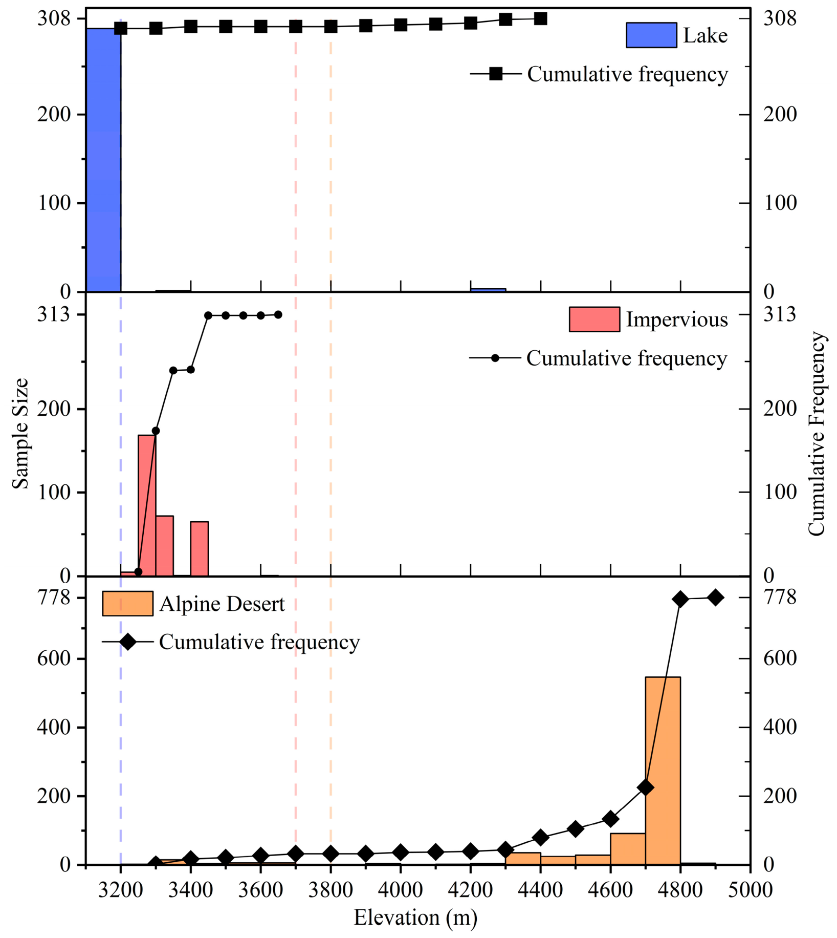
Furthermore, these elevation intervals were introduced as prior-guided auxiliary features rather than strict rule-based masks. The three elevation intervals in this study were determined through quantitative analysis of the class-wise elevation distributions of training samples for elevation-sensitive LULC. Elevation histograms and cumulative frequency revealed dominant concentration ranges where class probability increases significantly and inter-class overlap decreases (Figure 12). For example, alpine desert samples showed a strong concentration above 3800 m, with only 4.24% occurring below this elevation, whereas impervious surfaces were primarily distributed below 3700 m. Similarly, most lake samples occurred below 3200 m, which helps distinguish lakes from river channels in transitional zones.

We found that implementing elevation zones is more effective than only using DEM as an input variable. When raw DEM data were used without elevation-based thresholding, we observed a significant misclassification of natural vegetation as cropland—a phenomenon also evident in the TPLCD product within the QLB [12].

5.2. Area-Weighted Accuracy Assessment

Table 10 lists the area-weighted accuracy metrics following the method introduced in Section 3.3, with an area-weighted overall accuracy (OA_w) for the QLB of 81.50 ± 2.09% (95% confidence interval), revealing a 9.74% discrepancy from the unweighted sample-based OA (91.24%).

Area weighting rescales the entries of the confusion matrix by the mapped area of each class, which makes the disproportionate influence of small-area classes visible; however, it adjusts only for class-area proportions and cannot correct for the way in which the reference samples were located. Because our samples were collected through a purposive, non-probability design, the conditions required for design-based, unbiased inference are not met. The OA_w reported here, therefore, remains an apparent accuracy. Its departure from the sample-based OA reflects not only class-area imbalance, but also a component of spatial selection bias that we were unable to quantify with the present data.

The area-weighted apparent PA (PA_w) for small-area classes such as cropland and impervious surfaces dropped from 92.97% to 49.79%, and 95.45% to 41.56%, respectively. Conversely, the PA_w for the dominant alpine steppe increased from 68.84% to 79.15%. These variations suggest that once class areas are taken into account, the omission error may be lower than the unweighted sample-based classification suggested.

For large-area classes, a few misclassified pixels have a minimal impact on the total error because of their massive coverage. However, for small-area classes, misclassifying even a few pixels into dominant classes can substantially magnify their apparent omission error once class areas are taken into account. Therefore, to obtain truly unbiased, generalizable population estimates, future work should adopt a probability sampling design.

Beyond mapping accuracy, the proposed multisource data integration method provides a foundational data product for regional database construction and spatial governance. Our study draws inspiration from recent advancements in multi-source data-driven spatial identification and governance [59]. Looking forward, the QLBLC-10 dataset can be directly integrated into geographic information databases to support comprehensive downstream applications. Specifically, this high-resolution spatial information will enable the ecological monitoring of alpine grassland degradation, and facilitate environmental-effect assessments under climate change in the QLB.

6. Conclusions

In this study, an up-to-date (2024) LULC dataset (QLBLC-10) with a 10-m spatial resolution was generated for the QLB using multiseason optical, SAR, and topographic data. An SVM classifier was used to produce the QLBLC-10 at two hierarchical levels, achieving sample-based apparent overall accuracies of 91.95% (QLBLC-10-L1) and 91.24% (QLBLC-10-L2). An area-weighted overall accuracy of 81.50 ± 2.09% (95% confidence interval) was also computed, thereby clarifying the map-level uncertainties inherently associated with small-area classes. The multisource integration improved the sample-based apparent overall accuracy from 77.07% with single-season Sentinel-2 imagery to 91.24% with the full multisource feature set. While this multisource data fusion strategy provides a potential reference for mapping similar alpine environments, the classification scheme was tailored to the ecological and geomorphological characteristics of the QLB, aiming to capture the regional distribution of major alpine vegetation types. The resulting dataset serves as a possible data resource for regional ecological assessment and land management in the QLB. The main conclusions are as follows:

(1) Seasonal, multitemporal Sentinel-2 features substantially reduced confusion among vegetation types with similar phenological characteristics, enabling effective discrimination among temperate steppes, alpine steppes, and alpine meadows.

(2) Integrating C-band dual-polarization Sentinel-1 backscatter provided complementary structural information, improving the classification of alpine meadows, shrublands, croplands, and impervious surfaces.

(3) In regions characterized by strong elevation gradients, misclassifications between topographically segregated categories are mitigated by incorporating elevation intervals as auxiliary variables.

References

1. Jiang, T.; Jia, G.; Yu, X.; Zhang, T.; Feng, Y. Hydrologic Response to Extreme Climate Change in the Qinghai Lake Basin. Ecol. Indic. 2025, 178, 114048. [Google Scholar] [CrossRef] [Scilit]
2. Liu, K.; Li, N.; Liang, S. Prediction of Qinghai Lake’s Level under Future Climate Change: A Hybrid Modeling Approach Based on Hydrological Model and Deep Learning Method. J. Hydrol. Reg. Stud. 2025, 58, 102283. [Google Scholar] [CrossRef] [Scilit]
3. Lian, X.; Qi, Y.; Wang, H.; Zhang, J.; Yang, R. Assessing Changes of Water Yield in Qinghai Lake Watershed of China. Water 2020, 12, 11. [Google Scholar] [CrossRef] [Scilit]
4. Chen, Z.; Gao, X.; Liu, Z.; Chen, K. Spatiotemporal Variation of Soil Erosion Characteristics in the Qinghai Lake Basin Based on the InVEST Model. Int. J. Environ. Res. Public Health 2023, 20, 4728. [Google Scholar] [CrossRef] [Scilit] [PubMed]
5. Gong, P.; Liu, H.; Zhang, M.; Li, C.; Wang, J.; Huang, H.; Clinton, N.; Ji, L.; Li, W.; Bai, Y.; et al. Stable Classification with Limited Sample: Transferring a 30-m Resolution Sample Set Collected in 2015 to Mapping 10-m Resolution Global Land Cover in 2017. Sci. Bull. 2019, 64, 370–373. [Google Scholar] [CrossRef] [Scilit] [PubMed]
6. Brown, C.F.; Brumby, S.P.; Guzder-Williams, B.; Birch, T.; Hyde, S.B.; Mazzariello, J.; Czerwinski, W.; Pasquarella, V.J.; Haertel, R.; Ilyushchenko, S.; et al. Dynamic World, Near Real-Time Global 10 m Land Use Land Cover Mapping. Sci. Data 2022, 9, 251. [Google Scholar] [CrossRef] [Scilit]
7. Zanaga, D.; Van De Kerchove, R.; Daems, D.; De Keersmaecker, W.; Brockmann, C.; Kirches, G.; Wevers, J.; Cartus, O.; Santoro, M.; Fritz, S.; et al. ESA WorldCover 10 m 2021 V200. Zenodo 2022. [Google Scholar] [CrossRef]
8. Gong, P.; Wang, J.; Huang, H. Stable Classification with Limited Samples in Global Land Cover Mapping: Theory and Experiments. Sci. Bull. 2024, 69, 1862–1865. [Google Scholar] [CrossRef] [Scilit] [PubMed]
9. Zhang, X.; Liu, L.; Zhao, T.; Zhang, W.; Guan, L.; Bai, M.; Chen, X. GLC_FCS10: A Global 10-m Land-Cover Dataset with a Fine Classification System from Sentinel-1 and Sentinel-2 Time-Series Data in Google Earth Engine. Earth Syst. Sci. Data Discuss. 2025, 17, 4039–4062. [Google Scholar] [CrossRef] [Scilit]
10. Loess Plateau Scientific Data Center. 30-Meter Resolution Land Cover Dataset of the Tibetan Plateau (2010); Loess Plateau Scientific Data Center: Beijing, China, 2021; Available online: http://www.geodata.cn/data/datadetails.html?dataguid=140153143370799 (accessed on 2 December 2025).
11. Zhou, X.; Han, T.; McCullum, K.; Wu, P. The Comparison of Machine Learning Techniques for Agricultural Land Use Classifications in the Prairies: A Case Study in Saskatchewan, Canada. Agric. Res. 2024, 14, 518–528. [Google Scholar] [CrossRef] [Scilit]
12. Li, S.; Ge, Q.; Sun, F.; Ji, Q.; Liu, W.; Liu, R.; Xu, D.; Tao, Z. Annual 30 m Land Cover Dataset on the Tibetan Plateau from 1990 to 2023. Sci. Data 2025, 12, 510. [Google Scholar] [CrossRef] [Scilit] [PubMed]
13. Loveland, T.R.; Reed, B.C.; Brown, J.F.; Ohlen, D.O.; Zhu, Z.; Yang, L.; Merchant, J.W. Development of a Global Land Cover Characteristics Database and IGBP DISCover from 1 Km AVHRR Data. Int. J. Remote Sens. 2000, 21, 1303–1330. [Google Scholar] [CrossRef] [Scilit]
14. Fu, B.; Liu, Y.; Zhao, W.; Feng, X.; Liu, S.; Miao, C.; Wang, X.; He, C.; Li, C.; Ye, A.; et al. Optimization for Qinghai-Xizang Plateau Ecological Security Barrier System. Bull. Chin. Acad. Sci. Chin. Version 2024, 39, 1882–1893. [Google Scholar] [CrossRef]
15. Mo, L.; Yu, X.; Feng, Y.; Jiang, T. Runoff Variations and Quantitative Analysis in the Qinghai Lake Basin Under Changing Environments. Hydrology 2025, 12, 94. [Google Scholar] [CrossRef] [Scilit]
16. Abdi, A.M. Land Cover and Land Use Classification Performance of Machine Learning Algorithms in a Boreal Landscape Using Sentinel-2 Data. GISci. Remote Sens. 2020, 57, 1–20. [Google Scholar] [CrossRef] [Scilit]
17. Almarines, N.R.; Hashimoto, S.; Pulhin, J.M.; Tiburan, C.L.; Magpantay, A.T.; Saito, O. Influence of Image Compositing and Multisource Data Fusion on Multitemporal Land Cover Mapping of Two Philippine Watersheds. Remote Sens. 2024, 16, 2167. [Google Scholar] [CrossRef] [Scilit]
18. Wang, S.; Zou, X.; Liu, Y.; Zhai, H.; Liu, Y.; Cao, T. Two-Stage Cascade Learning for Accurate Vegetation Coverage Estimation in Qilian County Using Sentinel-2 Satellite Data. Int. J. Remote Sens. 2025, 46, 3259–3280. [Google Scholar] [CrossRef] [Scilit]
19. Goral, M.; le Maire, G.; Scolforo, H.F.; Stape, J.L.; Miranda, E.N.; Silva, T.C.F.; Ferreira, V.B.; Féret, J.-B.; de Boissieu, F. Monitoring the Early Growth of Forest Plantations with Sentinel-2 Satellite Time-Series. Int. J. Remote Sens. 2025, 46, 3110–3136. [Google Scholar] [CrossRef] [Scilit]
20. Cui, Z.; Chen, S.; Hu, B.; Wang, N.; Zhai, J.; Peng, J.; Bai, Z. High-Accuracy Mapping of Soil Organic Carbon by Mining Sentinel-1/2 Radar and Optical Time-Series Data with Super Ensemble Model. Remote Sens. 2025, 17, 678. [Google Scholar] [CrossRef] [Scilit]
21. Yu, H.; Li, G.; Liu, H.; Zhu, S.; Xu, J.; Dong, W.; Li, C.; Shi, J. Synergistic Fusion of Sentinel-1 and Sentinel-2 for Global LULC Mapping: The Multimodal Network LULC-Former and Dynamic World+ Dataset. IEEE J. Sel. Top. Appl. Earth Obs. Remote Sens. 2026, 19, 2511–2524. [Google Scholar] [CrossRef] [Scilit]
22. Guo, H.; Sun, J.; Fan, Z.; Yu, Z.; Tian, F.; Mao, X.; Wang, L.; Wang, S.; Gong, W.; Mao, F.; et al. Discriminating Natural and Planted Forests in Subtropical China Using Sentinel-2 Imagery and Inventory Data at 10 m Resolution. Int. J. Appl. Earth Obs. Geoinf. 2026, 147, 105179. [Google Scholar] [CrossRef] [Scilit]
23. Tesfaye, W.; Elias, E.; Warkineh, B.; Tekalign, M.; Abebe, G. Modeling of Land Use and Land Cover Changes Using Google Earth Engine and Machine Learning Approach: Implications for Landscape Management. Environ. Syst. Res. 2024, 13, 31. [Google Scholar] [CrossRef] [Scilit]
24. Dahal, S.; Dangi, B.; B.C., M.K.; Bhattarai, R.K. Land Use and Land Cover Classification for Dang District Nepal Using Satellite Imagery and Machine Learning on Google Earth Engine. J. Geogr. Environ. Earth Sci. Int. 2024, 28, 52–66. [Google Scholar] [CrossRef] [Scilit]
25. Dodin, M.; Levavasseur, F.; Savoie, A.; Martin, L.; Vaudour, E. Farm-Scale Mapping of Compost and Digestate Spreadings from Sentinel-2 and Sentinel-1. Int. J. Appl. Earth Obs. Geoinf. 2025, 139, 104555. [Google Scholar] [CrossRef] [Scilit]
26. Wu, Y.; Wu, H.; Tang, X.; Lv, J.; Zhang, R. Research on Computer Multi Feature Fusion SVM Model Based on Remote Sensing Image Recognition and Low Energy System. Results Eng. 2025, 26, 104861. [Google Scholar] [CrossRef] [Scilit]
27. Ren, Z.; Niu, D.; Ma, P.; Wang, Y.; Wang, Z.; Fu, H.; Elser, J.J. C:N:P Stoichiometry and Nutrient Limitation of Stream Biofilms Impacted by Grassland Degradation on the Qinghai-Tibet Plateau. Biogeochemistry 2020, 150, 31–44. [Google Scholar] [CrossRef] [Scilit]
28. Wang, H.; Qi, Y.; Lian, X.; Zhang, J.; Yang, R.; Zhang, M. Effects of Climate Change and Land Use/Cover Change on the Volume of the Qinghai Lake in China. J. Arid Land 2022, 14, 245–261. [Google Scholar] [CrossRef] [Scilit]
29. Chen, Q.; Liu, W.; Huang, C. Long-Term 10 m Resolution Water Dynamics of Qinghai Lake and the Driving Factors. Water 2022, 14, 671. [Google Scholar] [CrossRef] [Scilit]
30. Lee, J.; Hong, S.; Lee, K.; Won, J. Accuracy Assessment of a Digital Elevation Model Constructed Using the KOMPSAT-5 Dataset. Remote Sens. 2025, 17, 826. [Google Scholar] [CrossRef] [Scilit]
31. See, L.; Schepaschenko, D.; Lesiv, M.; McCallum, I.; Fritz, S.; Comber, A.; Perger, C.; Schill, C.; Zhao, Y.; Maus, V.; et al. Building a Hybrid Land Cover Map with Crowdsourcing and Geographically Weighted Regression. ISPRS J. Photogramm. Remote Sens. 2015, 103, 48–56. [Google Scholar] [CrossRef] [Scilit]
32. Sun, W.; Ding, X.; Su, J.; Mu, X.; Zhang, Y.; Gao, P.; Zhao, G. Land Use and Cover Changes on the Loess Plateau: A Comparison of Six Global or National Land Use and Cover Datasets. Land Use Policy 2022, 119, 106165. [Google Scholar] [CrossRef] [Scilit]
33. Li, J.; Zhang, B.; Huang, X. A Hierarchical Category Structure Based Convolutional Recurrent Neural Network (HCS-ConvRNN) for Land-Cover Classification Using Dense MODIS Time-Series Data. Int. J. Appl. Earth Obs. Geoinf. 2022, 108, 102744. [Google Scholar] [CrossRef] [Scilit]
34. Cao, W.; Wu, Y.; Liu, J.; Yuan, Y.; Zhang, C.; Zhao, S.; Wang, P. Seasonal Variation and Key Factors Influencing Evapotranspiration Partitioning in Alpine Ecosystems of the Qinghai Lake Basin. Ecol. Indic. 2025, 177, 113774. [Google Scholar] [CrossRef] [Scilit]
35. Amini, S.; Saber, M.; Rabiei-Dastjerdi, H.; Homayouni, S. Urban Land Use and Land Cover Change Analysis Using Random Forest Classification of Landsat Time Series. Remote Sens. 2022, 14, 2654. [Google Scholar] [CrossRef] [Scilit]
36. Daviran, M.; Maghsoudi, A.; Ghezelbash, R. Optimized AI-MPM: Application of PSO for Tuning the Hyperparameters of SVM and RF Algorithms. Comput. Geosci. 2025, 195, 105785. [Google Scholar] [CrossRef] [Scilit]
37. Mountrakis, G.; Im, J.; Ogole, C. Support Vector Machines in Remote Sensing: A Review. ISPRS J. Photogramm. Remote Sens. 2011, 66, 247–259. [Google Scholar] [CrossRef] [Scilit]
38. Duro, D.C.; Franklin, S.E.; Dubé, M.G. A Comparison of Pixel-Based and Object-Based Image Analysis with Selected Machine Learning Algorithms for the Classification of Agricultural Landscapes Using SPOT-5 HRG Imagery. Remote Sens. Environ. 2012, 118, 259–272. [Google Scholar] [CrossRef] [Scilit]
39. Huang, X.; Lu, Q.; Zhang, L.; Plaza, A. New Postprocessing Methods for Remote Sensing Image Classification: A Systematic Study. IEEE Trans. Geosci. Remote Sens. 2014, 52, 7140–7159. [Google Scholar] [CrossRef] [Scilit]
40. Maleki, R.; Wu, F.; Qu, G.; Liu, Y.; Oubara, A.; Yang, G. Integrating Image Filters and Confidence Thresholds to Improve Cropland Data Layer for Deep Learning–Based Cropland Segmentation. Eur. J. Remote Sens. 2026, 59, 2631928. [Google Scholar] [CrossRef] [Scilit]
41. Huang, D.; Xu, S.; Sun, J.; Liang, S.; Song, W.; Wang, Z. Accuracy Assessment Model for Classification Result of Remote Sensing Image Based on Spatial Sampling. J. Appl. Remote Sens. 2017, 11, 046023. [Google Scholar] [CrossRef] [Scilit]
42. Tola, D.D.; Dararo, K.F.; Manugula, S.S.; Dejene, I.N. Land Use/Cover Change and Its Correlation with Land Surface Temperature: The Case of Asella and Its Surrounding Area, Ethiopia. Ecol. Front. 2026; in press. [CrossRef] [Scilit]
43. Wassie, S.B.; Biru, B.Z.; Siraw, Z.; Talema, M.; Asichenek, A.; Belay, T. Detecting Land Use and Land Cover Changes and Quantifying Soil Erosion and Sediment Export Using GIS and Remote Sensing in the GERD Catchment, Ethiopia. Int. Soil Water Conserv. Res. 2026; in press. [CrossRef] [Scilit]
44. Olofsson, P.; Foody, G.M.; Herold, M.; Stehman, S.V.; Woodcock, C.E.; Wulder, M.A. Good Practices for Estimating Area and Assessing Accuracy of Land Change. Remote Sens. Environ. 2014, 148, 42–57. [Google Scholar] [CrossRef] [Scilit]
45. Dymond, J.R.; Shepherd, J.D.; Law, R.; Martin, B.; Schindler, J.; Belliss, S. A Cost-Effective Method for Mapping Land Cover at National Scale. Sci. Remote Sens. 2026, 13, 100376. [Google Scholar] [CrossRef] [Scilit]
46. Foody, G.M. Thematic Map Comparison. Photogramm. Eng. Remote Sens. 2004, 70, 627–633. [Google Scholar] [CrossRef] [Scilit]
47. Zhang, F.; Wang, X.; Xin, L.; Li, X. Assessing the Accuracy and Consistency of Cropland Datasets and Their Influencing Factors on the Tibetan Plateau. Remote Sens. 2025, 17, 1866. [Google Scholar] [CrossRef] [Scilit]
48. Hu, J.; Fan, D.; Tang, B.-H.; Zhu, X.-M. A New Model Incorporating Soil–Vegetation Interaction Scattering for Improving SAR-Based Soil Moisture Retrieval in Croplands. Remote Sens. 2026, 18, 673. [Google Scholar] [CrossRef] [Scilit]
49. Ibañez, D.; Xia, J.; Yokoya, N.; Pla, F.; Fernandez-Beltran, R. Inter-Sensor High-Resolution and Multi-Temporal Image Fusion for Unsupervised Domain Adaptation in Remote Sensing. IEEE Trans. Geosci. Remote Sens. 2025, 63, 1–23. [Google Scholar] [CrossRef] [Scilit]
50. Chen, Z.; Gao, X.; Liu, Z.; Sun, Y.; Chen, K. Spatiotemporal Evolution and Driving Mechanisms of Eco-Environmental Quality in a Typical Inland Lake Basin of the Northeastern Tibetan Plateau: A Case Study of the Qinghai Lake Basin. Land 2025, 14, 1955. [Google Scholar] [CrossRef] [Scilit]
51. Fang, P.; Wang, J.; Xu, H.; Li, R.; Yu, L.; Huang, S.; Liang, Y.; Zheng, P. Enhanced Supervised Classification of Seasonal Pastures on the Qinghai-Tibet Plateau (1990–2020) Using Landsat Optimal Time Window. GISci. Remote Sens. 2025, 62, 2530310. [Google Scholar] [CrossRef]
52. Alam, M.M. Unveiling Serverless: A Systematic Review of Software Architectures. In Proceedings of the 2024 International Conference on Advanced Information Scientific Development (ICAISD), West Java, Indonesia, 25–26 November 2024; pp. 58–63. [Google Scholar]
53. Pratama, B.A.S.; Danoedoro, P.; Arjasakusuma, S. Exploring Optimal Integration Schemes for Sentinel-1 SAR and Sentinel-2 Multispectral Data in Land Cover Mapping across Different Atmospheric Conditions. Remote Sens. Appl. Soc. Environ. 2024, 34, 101185. [Google Scholar] [CrossRef] [Scilit]
54. Dagne, S.S.; Hirpha, H.H.; Tekoye, A.T.; Dessie, Y.B.; Endeshaw, A.A. Fusion of Sentinel-1 SAR and Sentinel-2 MSI Data for Accurate Urban Land Use-Land Cover Classification in Gondar City, Ethiopia. Environ. Syst. Res. 2023, 12, 40. [Google Scholar] [CrossRef] [Scilit]
55. Zhang, H.; Yu, A.; Gao, K.; Lu, X.; Cao, X.; Guo, W.; Lian, W. M2Caps: Learning Multi-Modal Capsules of Optical and SAR Images for Land Cover Classification. Int. J. Digit. Earth 2025, 18, 2447347. [Google Scholar] [CrossRef] [Scilit]
56. Sun, J.; Ding, Y.; Wang, Y.; E, C. Vegetation Dynamics and Its Driving Force in the Qinghai Lake Basin, China. Front. Plant Sci. 2025, 16, 1691672. [Google Scholar] [CrossRef] [Scilit] [PubMed]
57. Jin, X.; Deng, A.; Fan, Y.; Ma, K.; Zhao, Y.; Wang, Y.; Zheng, K.; Zhou, X.; Lu, G. Diversity, Functionality, and Stability: Shaping Ecosystem Multifunctionality in the Successional Sequences of Alpine Meadows and Alpine Steppes on the Qinghai-Tibet Plateau. Front. Plant Sci. 2025, 16, 1436439. [Google Scholar] [CrossRef] [Scilit] [PubMed]
58. Wang, S.; Ma, L.; Yang, L.; Long, X.; Guan, C.; Zhao, C.; Chen, N. Quantifying Desertification in the Qinghai Lake Basin. Front. Environ. Sci. 2024, 12, 1309757. [Google Scholar] [CrossRef] [Scilit]
59. Ding, D.; Zhang, H.; Cao, Y.; Wang, D.; Sun, S.; Ding, D.; Zhang, H.; Cao, Y.; Wang, D.; Sun, S. Multi-Source Data-Driven Brownfield Identification: Methodology and Spatial Characteristics of Third Line Construction Cities. Urban Build. Sci. 2026, 2, 5. [Google Scholar] [CrossRef] [Scilit]
Figure 1. Study area. (a) Location of the study area on the Qinghai–Tibet Plateau; (b) Sentinel-2 RGB composite image of the Qinghai Lake Basin in August 2024 with field sampling site distributions within the basin; (c) temperate steppe; (d) alpine steppe; (e) alpine meadow; and (f) alpine shrubland. Here, (c1f1) were photographed during a field survey in October 2024, and (c2f2) are the corresponding Google Earth images.
Remotesensing 18 02353 g001
Figure 2. Workflow of the 2024 LULC classification in the Qinghai Lake Basin.
Remotesensing 18 02353 g002
Figure 3. (a) S2s-derived map; (b) S2t-derived map; (c) S2t + S1t-derived map; (d) S2t + S1t + DEM-derived map; (a1d1) local magnified areas in black boxes; (a2d2) local magnified areas in red boxes; (a3d3) local magnified areas in white boxes.
Remotesensing 18 02353 g003
Figure 4. Comparison of optical reflectance and radar backscatter characteristics of pixels misclassified using Sentinel-2 imagery but correctly reclassified as alpine meadows after the integration of Sentinel-1 data. (a) B4 surface reflectance; (b) B8 surface reflectance; (c) NDVI; (d) VV backscatter coefficient; (e) VH backscatter coefficient; (f) RVI.
Remotesensing 18 02353 g004
Figure 5. Level-1 LULC classification map (QLBLC-10-L1) in the Qinghai Lake Basin for 2024.
Remotesensing 18 02353 g005
Figure 6. Level-2 LULC classification map (QLBLC-10-L2) in the Qinghai Lake Basin for 2024.
Remotesensing 18 02353 g006
Figure 7. Area statistics of each LULC type in QLBLC-10-L1 and QLBLC-10-L2.
Remotesensing 18 02353 g007
Figure 8. CM for evaluating correct and incorrect samples in the Level-1 LULC category. Note: Both the x- and y-axes represent the Level-1 LULC category codes: 10—Grassland; 20—Shrubland; 30—Water; 40—Barren; 50—Wetland; 60—Cropland; 70—Impervious; and 80—Snow/Ice.
Remotesensing 18 02353 g008
Figure 9. CM for evaluating correct and incorrect samples in the Level-2 LULC category. Note: Both the x- and y-axes represent the Level-2 LULC category codes: 11—Temperate Steppe; 12—Alpine Steppe; 13—Alpine Meadow; 20—Alpine Shrubland; 31—Lake; 32—River; 41—Alpine Desert; 42—Sand Dunes; 43—River Beach; 50—Alpine Wetland; 60—Cropland; 70—Impervious; and 80—Snow/Ice.
Remotesensing 18 02353 g009
Figure 10. Comparison with (a) QLBLC-10-L1; (b) FROM-GLC10; (c) GLC-FCS10; and (d) TPLCD based on the unified classification system.
Remotesensing 18 02353 g010
Figure 11. Visual comparison of QLBLC-10-L2 with Google Earth imagery, FROM-GLC10, GLC-FCS10, and TPLCD: (af) Four typical areas were selected for close-up comparison.
Remotesensing 18 02353 g011
Figure 12. Elevation histograms and cumulative frequency based on sample counts for representative elevation-sensitive classes were used to determine DEM-based auxiliary intervals. Vertical dashed lines indicate selected reference elevations.
Remotesensing 18 02353 g012