Spectral-Prior-Guided Swin TransUnet for Sparse-Aperture FMCW MIMO-SAR Imaging

Highlights

What are the main findings?

• A spectral-prior-guided Swin TransUnet is proposed for sparse-aperture FMCW MIMO-SAR imaging by combining spectral priors, Swin Transformer-based ambiguity modeling, and multiscale feature fusion.
• The proposed method effectively suppresses azimuth grating lobes and reconstructs multiple point targets under 60% sparse-aperture sampling, achieving an RMSE below ${10}^{-2}$ and an azimuth ambiguity suppression ratio better than −30 dB when the SNR is higher than −6 dB.

What are the implications of the main findings?

• The method provides a feasible solution for high-quality range–azimuth imaging when platform motion leads to sparse synthetic-aperture sampling and azimuth ambiguity.
• The simulation and 77 GHz measured-data results indicate its potential for compact millimeter-wave radar imaging under sparse-aperture sampling.

Abstract

In millimeter-wave frequency-modulated continuous-wave (FMCW) multiple-input multiple-output synthetic-aperture radar (MIMO-SAR) imaging, platform displacement beyond the spatial Nyquist limit during a slow-time sampling interval creates aperture gaps, causing azimuth aliasing and degraded resolution. This paper proposes a spectral-prior-guided Swin TransUnet (SSTU) method for suppressing azimuth ambiguity in sparse moving-array imaging. Gaussian soft labels derived from point-scatterer positions formulate localization as heatmap regression and guide mainlobe learning. A two-dimensional fast Fourier transform (2D-FFT) layer then constructs a range–azimuth spectrum that exposes main peaks, sidelobes, and periodic grating lobes. A convolutional encoder extracts local spectral features, Swin Transformer blocks model long-range ambiguity correlations, and a U-Net-style multiscale decoder reconstructs high-resolution range–azimuth images. Simulations show that SSTU reliably recovers multiple point targets from noise and grating lobes despite substantial aperture gaps. At 60% aperture sparsity and signal-to-noise ratio (SNR) above −6 dB, it achieves a root mean square error (RMSE) below ${10}^{-2}$ and an azimuth ambiguity suppression ratio better than −30 dB, outperforming conventional methods. Measurements using a 77 GHz radar platform further demonstrate high-quality outdoor imaging of randomly distributed strong scatterers at 60% moving-aperture sparsity.

1. Introduction

High-resolution radar imaging is an important technology for short-range perception, target recognition, and environmental sensing and has been widely used in remote sensing [1,2], autonomous driving [3,4], and precision guidance [5]. However, on unmanned, vehicle-mounted, and missile-borne platforms, the antenna aperture, number of radio-frequency channels, and system cost are subject to strict constraints, making high-resolution imaging systems that rely on large-scale arrays difficult to deploy directly. With the rapid development of millimeter-wave radio-frequency devices and embedded signal processors, millimeter-wave FMCW radar can provide large bandwidth and high range resolution with small system volume and low power consumption and has become a reliable solution for high-resolution radar imaging on small platforms [6,7]. Nevertheless, owing to the limited physical aperture and limited number of transmit-receive channels, a single real-aperture observation is usually unable to provide sufficient azimuth resolution and spatial coverage simultaneously. To overcome this limitation, MIMO-SAR combines the multichannel spatial sampling capability of MIMO arrays with the motion-induced aperture synthesis mechanism of SAR. It can form more equivalent phase centers and extend the effective observation aperture under a limited number of physical elements, thereby providing a feasible route for compact high-resolution radar imaging [8,9,10].

Existing studies on MIMO-SAR imaging systems can be broadly grouped into array-structure design and imaging-method research. Array-structure design focuses on improving the equivalent-aperture utilization and spatial-frequency coverage under limited channel conditions by optimizing transmit schemes and array topologies. A new MIMO-SAR transmission scheme was designed in [11] to recover repeated equivalent phase centers and improve aperture utilization; FDM-MIMO was introduced into spaceborne SAR tomography in [12], where minimum-redundancy wavenumber-domain coverage was constructed to improve vertical wavenumber sampling efficiency; a compressive-sensing-based array synthesis model was introduced for wideband near-field millimeter-wave imaging in [13], achieving a trade-off between the number of array elements and aperture coverage; sparse arrays for three-dimensional near-field imaging can also be designed through convex optimization to improve sparse-aperture focusing performance [14].

Imaging method research, by contrast, aims to improve the resolution, focusing quality, and real-time processing capability of MIMO-SAR images under limited-aperture and complex observation conditions. For high-resolution wide-swath MIMO-SAR imaging, transmit delays and wide-null beamforming were introduced in [15] to realize echo separation and range ambiguity suppression; range resolution enhancement was used in [16] to compensate for the range-focusing limitations imposed by the system bandwidth and hardware conditions of miniature dechirped millimeter-wave MIMO-SAR; different processing schemes for automotive MIMO-SAR were compared in [17], providing an implementation basis for low-complexity range–azimuth imaging; Doppler-division multiplexing combined with multichannel back-projection was adopted in [18] to improve image focusing for automotive millimeter-wave MIMO-SAR; sparse and low-rank constraints were introduced in [19] for MIMO radar forward-looking super-resolution imaging, improving robust imaging capability under strong noise.

The above studies have investigated the structure and signal-processing algorithms of MIMO-SAR imaging in depth, but most of them assume that the equivalent aperture satisfies the spatial Nyquist sampling condition. When the platform displacement within a slow-time sampling interval exceeds the spatial Nyquist constraint, gaps appear in the equivalent aperture and lead to azimuth ambiguity [20,21,22]. For example, when an imaging system is deployed on a high-speed unmanned aerial or missile-borne platform, the slow-time sampling interval has a lower bound imposed by range resolution requirements, and rapid platform motion can make the equivalent synthetic aperture insufficiently sampled. To address imaging degradation caused by aperture undersampling, compressive sensing can exploit the sparse or compressible distribution of strong scattering centers in radar images to reconstruct sparse-aperture MIMO-SAR images, thereby improving image focusing quality and suppressing part of the artifacts under limited observations [23,24]. Compressive sensing was introduced into near-field radar imaging in [25] for image recovery under limited observations; the fast multipole method was embedded into near-field MIMO radar sparse reconstruction in [26], reducing the storage and computational burden caused by large-scale sensing matrices; and ${\mathcal{l}}_1$-norm minimization was applied to nonuniformly sampled FMCW SAR image reconstruction in [27], providing an evaluation basis for sparse regularized imaging.

However, compressive sensing methods are sensitive to SNR and aperture sparsity. When low SNR and high sparsity are coupled, insufficient effective observations weaken the stability of sparse inversion and reduce the separability between true targets and ambiguous targets. Compared with conventional model-driven methods, deep-learning methods can learn nonlinear mappings from degraded observations to high-quality images from data and have stronger representation capability for complex sidelobes and noise. They have therefore been increasingly applied to MIMO-SAR and millimeter-wave radar imaging. RMIST-Net combines a range migration model with a sparse reconstruction network to jointly exploit the physical propagation model and data-driven reconstruction capability [28]; cascaded physical back-projection and deep networks were used in [29] to realize real-time three-dimensional near-field MIMO imaging and improve reconstruction efficiency.

Learning-based imaging for moving sparse-aperture MIMO-SAR remains relatively limited. Inspired by the above studies, this paper develops a MIMO-SAR image reconstruction method based on a Transformer backbone and a U-Net feature-fusion architecture to reconstruct target range–azimuth images under sparse-aperture conditions. The main contributions and innovations of this paper are summarized as follows:

1.

To address grid mismatch in conventional discrete-grid imaging and the sidelobe effect introduced by the point spread function (PSF), two-dimensional Gaussian soft labels are constructed as training ground truth. Continuous target parameters are mapped onto the discrete grid through a Gaussian kernel, guiding the network to implicitly learn nonlinear deconvolution during training, enhancing sidelobe suppression, and improving imaging resolution.

2.

To address azimuth ambiguity caused by sparse sampling and SNR degradation, a spectral-prior-guided SSTU sparse-aperture MIMO-SAR image reconstruction network is proposed. Dechirped complex echoes are first converted into a range–azimuth spectrum, preserving the mainlobe, sidelobe, and periodic grating lobe structures induced by sparse-aperture sampling in the input feature space and providing a physically interpretable degradation prior for feature extraction. By combining convolutional feature extraction, window self-attention, and multiscale feature fusion, the proposed network reconstructs high-resolution, low-sidelobe range–azimuth images, thereby improving imaging accuracy and azimuth ambiguity suppression under sparse sampling.

3.

Within the above framework, simulations and 77 GHz radar field experiments are conducted to comprehensively evaluate imaging accuracy, ambiguity suppression, and computational efficiency. Simulation results show that the proposed method can image both simulated multiple point targets and measured point targets when the aperture sparsity reaches 60%. When the SNR is not lower than $-6$ dB, the azimuth ambiguity suppression ratio (AASR) is better than $-30$ dB, outperforming conventional algorithms. The five-point-target field experiment further validates the effectiveness of the proposed method on measured data.

The remainder of this paper is organized as follows. Section 2 describes the system model, azimuth ambiguity mechanism, and SSTU-based image reconstruction method. Section 3 presents the simulation and measured-data results. Section 4 discusses the ablation analysis, robustness to position errors, computational efficiency, applicability, and limitations. Finally, Section 5 concludes this paper.

2. Materials and Methods

2.1. Sparse Moving-Array Imaging Model

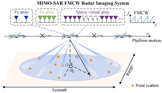
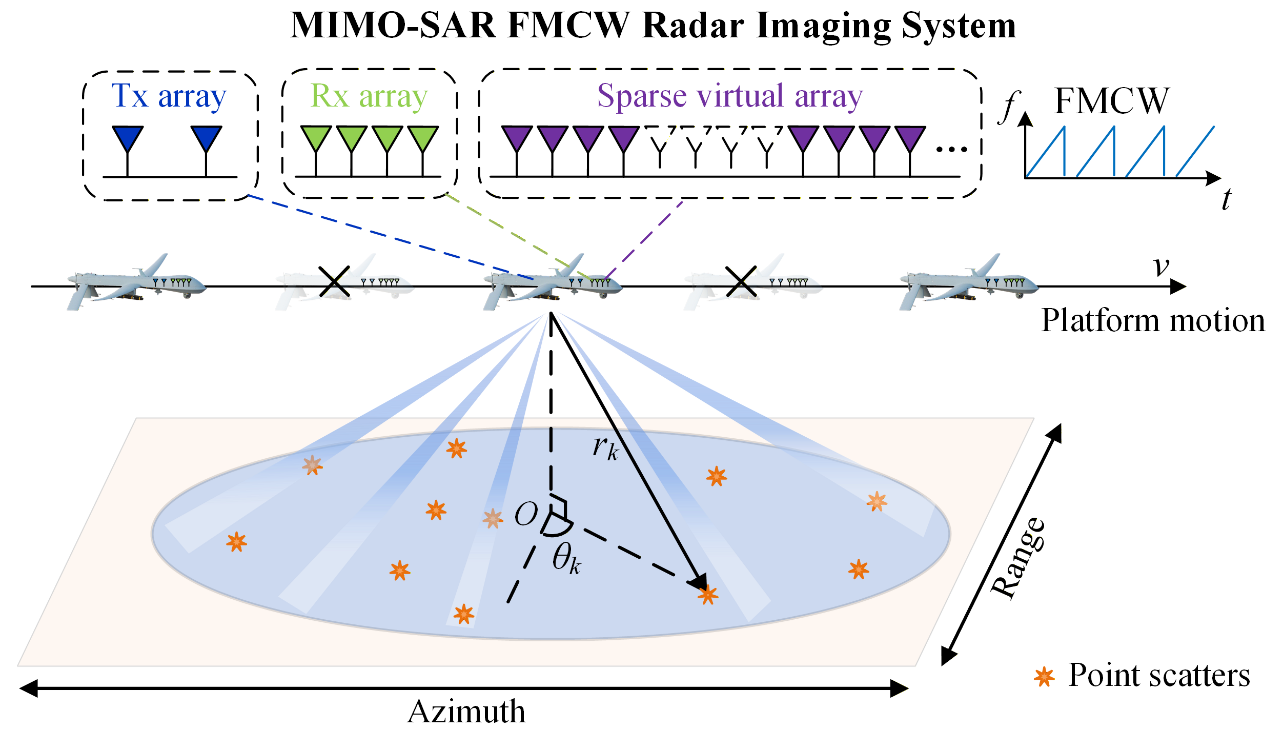
Consider a MIMO linear-array radar mounted on a moving platform, as illustrated in Figure 1. The platform moves uniformly along the azimuth direction with velocity v. The array consists of M transmit elements and N receive elements. The receive-element spacing is $d=\lambda /2$, and the transmit-element spacing is $Nd$, where $\lambda$ is the carrier wavelength.

Figure 1. Geometry of the sparse moving-array FMCW MIMO-SAR imaging model.

With the initial array position as the origin, the azimuth coordinates of the mth transmit element and the nth receive element are

$$\begin{array}{c}{x}_{t,m}=mNd,m=0,\dots ,M-1,\\ x_{r,n}=nd,n=0,\dots ,N-1.\end{array}$$

(1)

The azimuth coordinate associated with the $(m,n)$ transmit-receive channel is

$$p_{m,n}=x_{t,m}+x_{r,n}.$$

(2)

Thus, one MIMO snapshot, corresponding to one azimuth slow-time sampling position, forms $MN$ uniformly spaced virtual-array elements. Let $T_p$ denote the slow-time sampling interval between adjacent MIMO snapshots. The platform displacement between two adjacent MIMO snapshots is

$$\Delta =v{T}_p.$$

(3)

For a TDM-MIMO acquisition, the array coherently acquires L MIMO snapshots within the coherent processing aperture. Assuming that the small platform displacement during the fast-time sampling interval of a single chirp and the intra-group displacement during transmit-channel switching are negligible or have been corrected by motion compensation, the virtual-array coordinate associated with the $(m,n)$ transmit–receive pair in the lth MIMO snapshot is

$$p_{l,m,n}=2l\Delta +p_{m,n},l=0,\dots ,L-1,m=0,\dots ,M-1,n=0,\dots ,N-1.$$

(4)

All virtual-array coordinates are then ordered as ${\left\{p_q\right\}}_{q=0}^{Q-1}$, where $Q=LMN$.

The transmitted FMCW signal within one chirp period can be written as

$$s_t\left(t\right)=\exp \left[j2\pi \left(f_{c}t+{\displaystyle \frac{1}{2}}K{t}^2\right)\right],0\le t<T_c,$$

(5)

where $f_c$ is the carrier frequency, $K=B/T_c$ is the chirp slope, and B and $T_c$ are the signal bandwidth and chirp duration, respectively. Suppose there are S point scatterers in the scene. The sth scatterer is located at $(r_s,{\theta }_s)$ in the range–azimuth domain and has scattering coefficient ${\sigma }_s$. For the qth virtual-array element, the equivalent one-way distance to this scatterer is

$$R_{q,s}=\sqrt{{\left(r_s\sin {\theta }_s-{\displaystyle \frac{p_q}{2}}\right)}^2+{\left(r_s\cos {\theta }_s\right)}^2}.$$

(6)

Under the equivalent phase-center approximation, the received echo of the qth virtual channel is the coherent superposition of all scatterer echoes:

$$r_q\left(t\right)={\displaystyle \sum _{s=1}^S}{\sigma }_s\exp \left[j2\pi \left(f_c(t-{\tau }_{q,s})+{\displaystyle \frac{1}{2}}K{\left(t-{\tau }_{q,s}\right)}^2\right)\right]+w_q\left(t\right),$$

(7)

where ${\tau }_{q,s}=2R_{q,s}/c$, c is the speed of light, and $w_q\left(t\right)$ denotes receiver noise. After dechirping and neglecting residual video phase and amplitude attenuation, the intermediate-frequency baseband signal is

$$y_q\left(t\right)={\displaystyle \sum _{s=1}^S}{\sigma }_s\exp \left[-j{\displaystyle \frac{4\pi f_c}{c}}{R}_{q,s}\right]\exp \left[-j{\displaystyle \frac{4\pi K}{c}}{R}_{q,s}t\right]+n_q\left(t\right).$$

(8)

The range–azimuth imaging region is discretized into P grid points. The ith grid point is denoted as $(r_i,{\theta }_i)$, with scattering coefficient ${\gamma }_i$. If the fast-time sampling rate is $f_s$, the fast-time instant corresponding to the kth sample is $k/f_s$, $k=0,\dots ,N_s-1$, where $N_s$ is the number of range samples. The dechirped echo at the qth virtual-array element and the kth fast-time sample can then be written as

$$\begin{array}{cc}\hfill y_q\left[k\right]& ={\displaystyle \sum _{i=1}^P}{\gamma }_i{a}_{q,i}\left[k\right]+n_q\left[k\right],\hfill \\ \hfill a_{q,i}\left[k\right]& =\exp \left[-j{\displaystyle \frac{4\pi f_c}{c}}{R}_{q,i}\right]\exp \left[-j{\displaystyle \frac{4\pi K}{c}}{R}_{q,i}{\displaystyle \frac{k}{f_s}}\right],\hfill \end{array}$$

(9)

where $R_{q,i}=\sqrt{{\left(r_i\sin {\theta }_i-p_q/2\right)}^2+{\left(r_i\cos {\theta }_i\right)}^2}$. The echoes over all virtual-array elements and fast-time samples form a two-dimensional discrete echo matrix

$$\mathbf{Y}={\left[y_q\left[k\right]\right]}_{\begin{array}{c}q=0,\dots ,Q-1\\ k=0,\dots ,N_s-1\end{array}}\in {\mathbb{C}}^{Q\times N_s}.$$

(10)

2.2. Azimuth Ambiguity

Between adjacent MIMO snapshots, the platform displacement $\Delta =v{T}_p$ translates the virtual array by $2\Delta$. The spacing between the last virtual-array element in the lth MIMO snapshot and the first virtual-array element in the $(l+1)$th MIMO snapshot is

$${\Delta }_p=2\Delta -(MN-1)d.$$

(11)

When ${\Delta }_p=d$, the aperture spacing between adjacent MIMO snapshots is consistent with the intra-snapshot virtual-array spacing, and the equivalent aperture forms continuous uniform azimuth sampling. When ${\Delta }_p>d$, aperture holes appear between adjacent MIMO snapshots, and the effective aperture becomes periodically sparse along slow time. When ${\Delta }_p<d$, the slow-time samples become redundant. This paper focuses on the sparse-aperture case with ${\Delta }_p>d$.

For the sth scatterer at $(r_s,{\theta }_s)$, the spatial phase corresponding to the qth virtual-array element is

$${\varphi }_{q,s}=-{\displaystyle \frac{4\pi }{\lambda }}{R}_{q,s}=-{\displaystyle \frac{4\pi }{\lambda }}\sqrt{{\left(r_s\sin {\theta }_s-{\displaystyle \frac{p_q}{2}}\right)}^2+{\left(r_s\cos {\theta }_s\right)}^2}.$$

(12)

For two adjacent virtual-array elements separated by ${\Delta }_p$ at the boundary between adjacent MIMO snapshots, a first-order Taylor expansion gives the approximate phase difference

$$\Delta {\varphi }_s\approx {\displaystyle \frac{2\pi }{\lambda }}{\displaystyle \frac{r_s\sin {\theta }_s-\frac{p_q}{2}}{R_{q,s}}}{\Delta }_p.$$

(13)

To avoid spatial-frequency aliasing in the aperture dimension, the phase variation between adjacent aperture samples should satisfy

$$|\Delta {\varphi }_s| \le \pi .$$

(14)

Thus, the non-aliased sampling condition is

$${\Delta }_p\le {\displaystyle \frac{\lambda }{2}}\left|{\displaystyle \frac{R_{q,s}}{r_s\sin {\theta }_s-\frac{p_q}{2}}}\right|.$$

(15)

Under the far-field or small-aperture approximation, $(r_s\sin {\theta }_s-p_q/2)/R_{q,s}\approx \sin {\theta }_s$, and the condition becomes

$${\Delta }_p\le {\displaystyle \frac{\lambda }{2|\sin {\theta }_s|}}.$$

(16)

Therefore, when ${\Delta }_p>\lambda /\left(2\right|\sin {\theta }_s\left|\right)$, the aperture phase sampling at the azimuth of the sth scatterer exceeds the spatial Nyquist constraint, and azimuth spatial-frequency aliasing occurs. As $|{\theta }_s|$ increases, the maximum allowable inter-snapshot aperture spacing decreases, so the same aperture holes more readily produce azimuth grating lobes and false peaks.

To further determine the locations and relative strengths of the grating-lobe components, the spectral-replication mechanism induced by periodic block-sparse sampling is analyzed in the Fourier domain.

When ${\Delta }_p>d$, the equivalent aperture can be regarded as periodic block sampling of a full-aperture uniform virtual-element grid with spacing d. Each MIMO snapshot occupies $MN$ consecutive grid positions, and J grid positions are missing between two adjacent MIMO snapshots. Therefore,

$${\Delta }_p=(J+1)d.$$

(17)

Combining this relation with the definition of ${\Delta }_p$ gives

$$2v{T}_p=(MN+J)d.$$

(18)

The above equation indicates that for a given slow-time sampling interval, the number of missing virtual elements J has a one-to-one correspondence with the platform velocity v. Therefore, J is used in the following sections to parameterize the sparsity level of the equivalent aperture.

Let $\tilde{q}$ denote the index of the full-aperture uniform grid. The sparse-aperture echo can be expressed as the product of the full uniformly sampled aperture echo and a binary sampling mask $\chi \left[\tilde{q}\right]$. The mask is the convolution between an intra-group contiguous block $b\left[\tilde{q}\right]$ and an impulse train with period $MN+J$, namely,

$$\begin{array}{cc}\hfill \chi \left[\tilde{q}\right]& ={\displaystyle \sum _{l=0}^{L-1}}b[\tilde{q}-l(MN+J)],\hfill \\ \hfill b\left[\tilde{q}\right]& =\left\{\begin{array}{cc}1,\hfill & 0\le \tilde{q}\le MN-1,\hfill \\ 0,\hfill & \mathrm{otherwise}.\hfill \end{array}\right.\hfill \end{array}$$

(19)

The normalized azimuth spatial frequency of the sth scatterer is $f_{a,s}=(d/\lambda )\sin {\theta }_s$. Since multiplication in the aperture domain corresponds to convolution in the spectral domain, and the azimuth spectrum of the periodic mask is a line spectrum with spacing $1/(MN+J)$ weighted by the Dirichlet envelope of the intra-group block, the target spectrum is replicated to $f_{a,s}+{\displaystyle \frac{\kappa }{MN+J}},\kappa =\pm 1,\pm 2,\dots$, which corresponds to periodic grating lobes in the angular domain. The amplitude ratio between the $\kappa$th replicated component and the main component is

$${\xi }_{\kappa }=\left|{\displaystyle \frac{\sin \left(\pi \kappa MN/(MN+J)\right)}{MN\sin \left(\pi \kappa /(MN+J)\right)}}\right|.$$

(20)

When $J=0$, ${\xi }_{\kappa }$ is zero within the field of view, and the equivalent aperture reduces to unambiguous uniform full sampling, so no azimuth ambiguity is generated. As J increases, the spectral-line spacing decreases and the envelope suppression weakens, making ambiguity peaks denser and stronger. Thus, the grating-lobe positions and amplitudes are fully determined by $MN$ and J. This structured and predictable mainlobe-grating-lobe pattern is explicitly revealed in the range-azimuth spectrum after zero filling and two-dimensional FFT, forming the spectral prior exploited by the proposed network.

2.3. Proposed Method

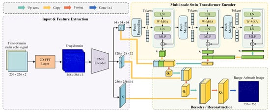
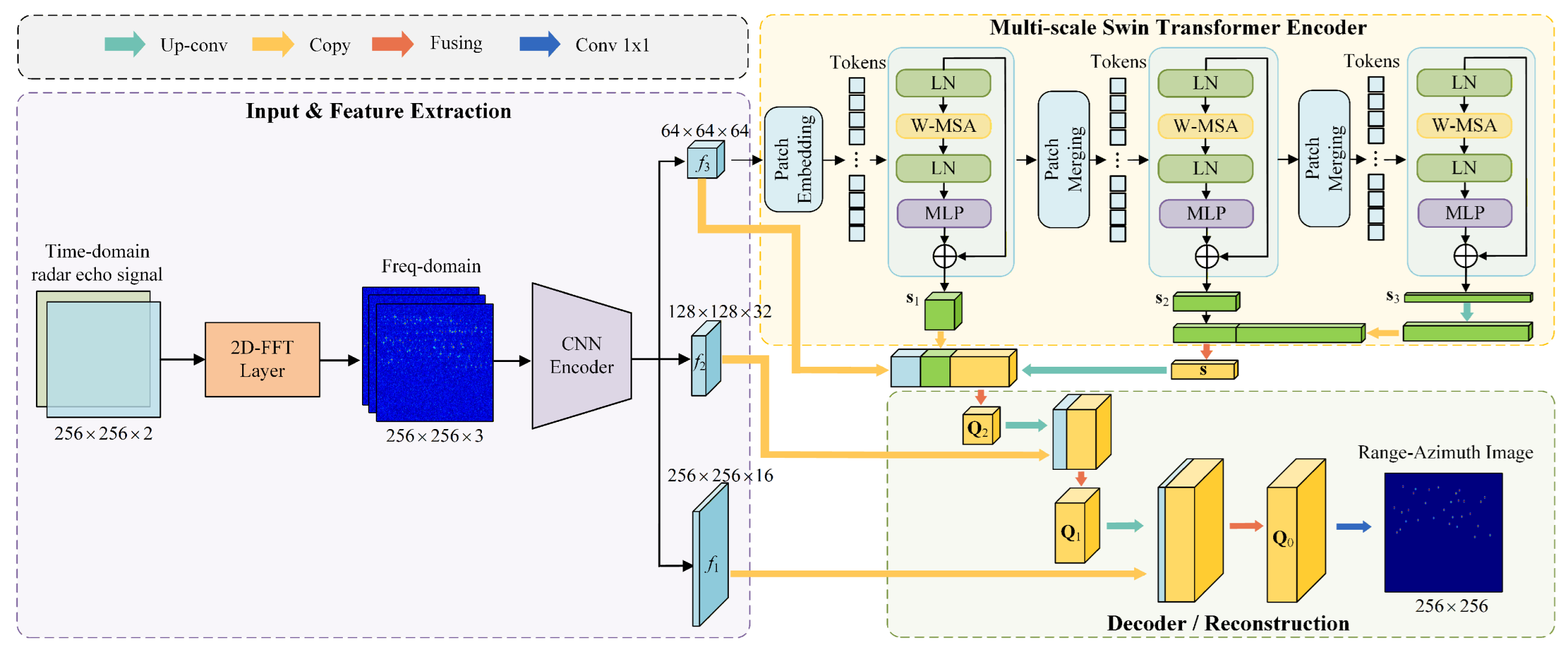
When the platform displacement between adjacent MIMO snapshots is large, sparse MIMO-SAR sampling produces dense periodic azimuth ambiguities. The degradation is particularly severe under low-SNR conditions, where the energy contrast between true mainlobes and false peaks becomes weak and amplitude-only discrimination is unreliable. To reduce the influence of ambiguity and reconstruct high-resolution target images, this work adopts a neural-network-based MIMO-SAR image reconstruction method. Sparse-array echoes are used as the input, and two-dimensional Gaussian-kernel mappings constructed from the true target range–azimuth coordinates are used as soft labels. A spectral-prior-guided SSTU fusion network is then developed to jointly suppress azimuth ambiguities and noise. The network flowchart is shown in Figure 2.

Figure 2. Architecture of the proposed spectral-prior-guided Swin TransUnet.

2.3.1. SSTU Network Architecture

(1)

2D-FFT Layer

The columns of the discrete echo matrix $\mathbf{Y}$ contain range beat-frequency modulation, whereas its rows contain azimuth phase modulation induced by the virtual-array coordinates $p_q$. Since the sparse moving aperture can be viewed as observations sampled from a uniform full-aperture azimuth grid, the measured echoes are first embedded into their corresponding full-aperture grid positions, while unobserved positions are filled with zeros. Let $\tilde{q}$ denote the row index of the full-aperture grid and let $N_a$ be the number of azimuth samples after zero filling. The zero-filled aperture echo matrix is then $\tilde{\mathbf{Y}}\in {\mathbb{C}}^{N_a\times N_s}$.

Define ${\mathbf{P}}_z\in {\{0,1\}}^{N_a\times Q}$ as the zero-filling rearrangement matrix. Its nonzero entries embed the Q actually observed channels into the $N_a$ uniform full-aperture azimuth grid, and unobserved grid positions correspond to zero rows in ${\mathbf{P}}_z$. The zero-filling operation is written as

$$\tilde{\mathbf{Y}}={\mathbf{P}}_z\mathbf{Y}.$$

(21)

The echo sample in the $\tilde{q}$th row and kth column of $\tilde{\mathbf{Y}}$ is therefore

$${\tilde{y}}_{\tilde{q}}\left[k\right]={\left[\tilde{\mathbf{Y}}\right]}_{\tilde{q},k}={\displaystyle \sum _{q=0}^{Q-1}}{\left[{\mathbf{P}}_z\right]}_{\tilde{q},q}{y}_q\left[k\right],\tilde{q}=0,\dots ,N_a-1,k=0,\dots ,N_s-1.$$

(22)

If the $\tilde{q}$th full-aperture grid position contains an observation, the above expression equals the corresponding channel echo; otherwise, ${\tilde{y}}_{\tilde{q}}\left[k\right]=0$.

For the $\tilde{q}$th row sequence ${\left\{{\tilde{y}}_{\tilde{q}}\left[k\right]\right\}}_{k=0}^{N_s-1}$, a $2N_r$-point range FFT is applied and the first $N_r$ range frequency bins are retained:

$$S_{\tilde{q}}\left(f_r\right)={\displaystyle \sum _{k=0}^{N_s-1}}{w}_r\left[k\right]{\tilde{y}}_{\tilde{q}}\left[k\right]\exp \left(-j2\pi f_{r}k\right),$$

(23)

where $f_r={\mathcal{l}}_r/\left(2N_r\right)$ is the normalized range frequency, ${\mathcal{l}}_r=0,\dots ,N_r-1$, and $w_r\left[k\right]$ is the range window function. After range FFTs are obtained for all full-aperture azimuth-grid positions, an $N_a$-point FFT is applied along the azimuth dimension for each range-frequency sample:

$$A(f_r,f_a)={\displaystyle \sum _{\tilde{q}=0}^{N_a-1}}{w}_a\left[\tilde{q}\right]S_{\tilde{q}}\left(f_r\right)\exp \left(-j2\pi f_a\tilde{q}\right),$$

(24)

where $f_a={\mathcal{l}}_a/N_a$ is the normalized azimuth frequency, ${\mathcal{l}}_a=0,\dots ,N_a-1$, and $w_a\left[\tilde{q}\right]$ is the azimuth window function. The samples $A(f_r,f_a)$ are arranged along the range- and azimuth frequency axes to form the range–azimuth spectrum $\mathbf{A}$.

In a full-aperture or uniformly sampled synthetic-aperture scenario, the two-dimensional FFT performs range compression and azimuth focusing. Under sparse platform motion, its output explicitly retains grating lobe and aliasing structures caused by aperture undersampling. Therefore, the 2D-FFT is used as the network front end to map the raw complex echoes to a physically interpretable range–azimuth spectrum. In this spectrum, the target mainlobes and periodic grating lobes, whose locations and relative amplitudes are determined by sparse-aperture sampling, are explicitly represented and constitute the spectral prior exploited by the network. This prior enables subsequent network modules to directly learn the structural differences among true peaks, sidelobes, and false peaks.

The two-dimensional FFT process can be written in operator form as

$$\mathbf{A}={\mathcal{F}}_a\left\{{\mathcal{F}}_r\left(\tilde{\mathbf{Y}}\right)\right\},$$

(25)

where ${\mathcal{F}}_r(·)$ denotes the $2N_r$-point discrete Fourier transform along the range dimension followed by retaining the first $N_r$ range frequency bins, ${\mathcal{F}}_a(·)$ denotes the $N_a$-point discrete Fourier transform along the azimuth dimension, and $\mathbf{A}\in {\mathbb{C}}^{N_r\times N_a}$ is the range–azimuth spectrum. The complex spectrum is decomposed into real, imaginary, and magnitude channels:

$$\mathbf{X}=\left[\mathrm{Re}\left(\mathbf{A}\right),\mathrm{Im}\left(\mathbf{A}\right),\left|\mathbf{A}\right|\right]\in {\mathbb{R}}^{3\times N_r\times N_a}.$$

(26)

The real and imaginary channels preserve coherent phase information in the spectral domain, while the magnitude channel describes the energy distribution of target mainlobes and azimuth ambiguities.

(2)

Convolutional Encoder

A CNN encoder receives the three-channel output of the 2D-FFT layer and extracts multiscale spectral features [30,31]. It is implemented as a progressive downsampling encoder with three convolutional blocks. The first convolutional block fuses the three 2D-FFT-derived spectral channels through two $3\times 3$ convolutional layers with ReLU activation and extracts local structures of target mainlobes, sidelobes, and the noise background. The following stages use stride-2 convolutions for downsampling, halve the feature resolution, expand the channel dimension, and enhance the representation of medium-scale azimuth ambiguity distributions. After progressive encoding, multiscale feature maps are obtained. Let ${\mathbf{F}}_0=\mathbf{X}$, and let the three encoder feature maps be ${\mathbf{F}}_1$, ${\mathbf{F}}_2$, and ${\mathbf{F}}_3$. The encoder is written as

$${\mathbf{F}}_i={\mathcal{C}}_i\left({\mathbf{F}}_{i-1}\right),i=1,2,3,$$

(27)

where ${\mathcal{C}}_1(·)$ consists of two $3\times 3$ convolutions with ReLU activation and performs local feature fusion at the original spectrum resolution. ${\mathcal{C}}_2(·)$ and ${\mathcal{C}}_3(·)$ denote convolutional mappings with downsampling; they use stride-2 $3\times 3$ convolutions to reduce spatial resolution, expand the channel dimension, and further extract local spectral structures in the downsampled feature spaces. The resulting feature maps have sizes

$${\mathbf{F}}_1\in {\mathbb{R}}^{C\times N_r\times N_a},{\mathbf{F}}_2\in {\mathbb{R}}^{2C\times {\displaystyle \frac{N_r}{2}}\times {\displaystyle \frac{N_a}{2}}},{\mathbf{F}}_3\in {\mathbb{R}}^{4C\times {\displaystyle \frac{N_r}{4}}\times {\displaystyle \frac{N_a}{4}}}.$$

(28)

Here, C denotes the base channel number. In sparse-aperture scenarios caused by large inter-snapshot displacement, this hierarchical encoding helps suppress noise and coherent artifacts while improving the contrast and resolution of the reconstructed image.

(3)

Swin Transformer

Sparse-aperture sampling produces azimuth grating lobes with a periodic distribution. After local spectral features are extracted by the convolutional encoder, a Swin Transformer is introduced to further model the relationship between mainlobes and grating lobes in the range–azimuth spectrum [32]. The input to the Swin Transformer is the bottleneck feature map ${\mathbf{F}}_3\in {\mathbb{R}}^{4C\times N_r/4\times N_a/4}$. Patch embedding $\mathcal{P}(·)$ divides ${\mathbf{F}}_3$ into non-overlapping patches of size $P_w\times P_w$ and maps each patch to a D-dimensional token. Let the numbers of patches along the range and azimuth directions be $H_f=N_r/\left(4P_w\right)$ and $W_f=N_a/\left(4P_w\right)$, respectively. The total number of tokens is $N_t=H_f{W}_f$, and the initial token sequence is

$${\mathbf{Z}}_0=\mathcal{P}\left({\mathbf{F}}_3\right)=\left[{\mathbf{z}}_1,{\mathbf{z}}_2,\dots ,{\mathbf{z}}_{N_t}\right]\in {\mathbb{R}}^{N_t\times D},$$

(29)

where ${\mathbf{z}}_i\in {\mathbb{R}}^D$.

The Swin Transformer is composed of multiple stages. Patch merging between stages decreases the spatial resolution and increases the channel dimension. For a layer u within a stage, let its input feature have spatial size $H_u\times W_u$ and channel dimension $D_u$:

$${\mathbf{Z}}^{\left(u\right)}\in {\mathbb{R}}^{H_u\times W_u\times D_u}.$$

(30)

Let $N_u=H_u{W}_u$ be the corresponding number of tokens. The feature is partitioned into local windows of size $M_w\times M_w$, giving $N_w=H_u{W}_u/M_w^2$ windows. The token feature matrix in the wth window is

$${\mathbf{Z}}_w^{\left(u\right)}=\left[{\mathbf{z}}_{w,1}^{\left(u\right)},{\mathbf{z}}_{w,2}^{\left(u\right)},\dots ,{\mathbf{z}}_{w,M_w^2}^{\left(u\right)}\right]\in {\mathbb{R}}^{M_w^2\times D_u},w=1,2,\dots ,N_w.$$

(31)

Within each local window, multi-head self-attention (MSA) is computed to model local spatial correlations [33,34]. The hth attention head is

$${\mathrm{Attn}}_h\left({\mathbf{Z}}_w^{\left(u\right)}\right)=\mathrm{Softmax}\left({\displaystyle \frac{{\mathbf{Q}}_h{\mathbf{K}}_h^{\top }}{\sqrt{d_h}}}+{\mathbf{B}}_{\mathrm{rel}}\right){\mathbf{V}}_h,$$

(32)

with

$${\mathbf{Q}}_h={\mathbf{Z}}_w^{\left(u\right)}{\mathbf{W}}_h^Q,{\mathbf{K}}_h={\mathbf{Z}}_w^{\left(u\right)}{\mathbf{W}}_h^K,{\mathbf{V}}_h={\mathbf{Z}}_w^{\left(u\right)}{\mathbf{W}}_h^V.$$

(33)

Here, ${\mathbf{B}}_{\mathrm{rel}}$ is the relative position bias and ${\mathbf{W}}_h^Q$, ${\mathbf{W}}_h^K$, and ${\mathbf{W}}_h^V\in {\mathbb{R}}^{D_u\times d_h}$ are learnable projection matrices, with $d_h=D_u/N_h$. The outputs of all $N_h$ heads are concatenated and linearly projected as

$${\mathbf{O}}_w^{\left(u\right)}=\left[{\mathrm{Attn}}_1\left({\mathbf{Z}}_w^{\left(u\right)}\right),{\mathrm{Attn}}_2\left({\mathbf{Z}}_w^{\left(u\right)}\right),\dots ,{\mathrm{Attn}}_{N_h}\left({\mathbf{Z}}_w^{\left(u\right)}\right)\right]{\mathbf{W}}^O,$$

(34)

where ${\mathbf{W}}^O\in {\mathbb{R}}^{D_u\times D_u}$ is the output projection matrix. Shifted windows are used in adjacent layers: windows remain fixed in one layer and are shifted by half a window in the next, enabling boundary features from neighboring windows to be jointly modeled and cross-region global dependencies to be captured without increasing the computational complexity. After the stages of window self-attention and patch merging, the Swin Transformer forms fine-to-coarse spectral degradation representations. The output tokens of the window-attention blocks at different stages are rearranged into two-dimensional feature maps with the corresponding spatial resolutions:

$${\mathbf{s}}_1\in {\mathbb{R}}^{D\times H_f\times W_f},{\mathbf{s}}_2\in {\mathbb{R}}^{2D\times {\displaystyle \frac{H_f}{2}}\times {\displaystyle \frac{W_f}{2}}},{\mathbf{s}}_3\in {\mathbb{R}}^{4D\times {\displaystyle \frac{H_f}{4}}\times {\displaystyle \frac{W_f}{4}}}.$$

(35)

(4)

Multiscale Fusion Decoder

The decoder follows a U-Net-like structure [35] and progressively restores the range-azimuth amplitude map by fusing convolutional local features and Swin Transformer features. At the coarsest scale, ${\mathbf{s}}_2$ and ${\mathbf{s}}_3$ are spatially aligned and concatenated:

$${\mathbf{s}}_0={\psi }_0\left(\left[{\mathbf{s}}_2,\mathcal{U}\left({\mathbf{s}}_3\right)\right]\right),$$

(36)

where $\mathcal{U}(·)$ denotes bilinear upsampling, $[·,·]$ denotes channel concatenation, and ${\psi }_0(·)$ is a two-layer $3\times 3$ convolutional fusion function with ReLU activation. The hierarchical reconstruction is then written as

$$\begin{array}{cc}\hfill {\mathbf{D}}_2& ={\psi }_1\left(\left[{\mathcal{U}}_3\left({\mathbf{s}}_0\right),{\mathcal{U}}_3\left({\mathbf{s}}_1\right),{\mathbf{F}}_3\right]\right),\hfill \\ \hfill {\mathbf{D}}_1& ={\psi }_2\left(\left[\mathcal{U}\left({\mathbf{D}}_2\right),{\mathbf{F}}_2\right]\right),\hfill \\ \hfill {\mathbf{D}}_0& ={\psi }_3\left(\left[\mathcal{U}\left({\mathbf{D}}_1\right),{\mathbf{F}}_1\right]\right),\hfill \end{array}$$

(37)

where ${\mathcal{U}}_3(·)$ upsamples Swin Transformer features to the spatial size of ${\mathbf{F}}_3$, ensuring that the concatenated feature maps are aligned in both the range and azimuth dimensions. The final amplitude prediction is obtained by a $1\times 1$ convolution:

$$\widehat{\mathbf{G}}=\mathrm{ReLU}\left({\mathrm{Conv}}_{1\times 1}\left({\mathbf{D}}_0\right)\right)\in {\mathbb{R}}^{N_r\times N_a}.$$

(38)

2.3.2. Gaussian-Kernel-Based Soft Target Labels

FFT- and back-projection (BP)-based imaging methods are limited by the system bandwidth and effective aperture. For an ideal point scatterer, the image-domain response is governed by the point spread function (PSF), which has a finite mainlobe width and sidelobe leakage in both range and azimuth. Windowing can reduce sidelobe levels, but it is often accompanied by mainlobe broadening and resolution loss, and the window parameters are scene-dependent. Moreover, real scattering centers lie in continuous space, whereas image labels are defined on discrete grids; single-pixel hard labels may therefore introduce grid mismatch and increase the difficulty of network optimization. To address this issue, Gaussian-kernel-based soft target labels are constructed on the same range–azimuth grid as the network output, providing continuous and smooth supervision, alleviating grid quantization error, and improving sidelobe suppression and resolution under limited-aperture conditions.

Specifically, on a label plane with $N_r$ range-grid points and $N_a$ azimuth-grid points, the continuous range–azimuth coordinate $(r_s,{\theta }_s)$ and amplitude weight ${\alpha }_s$ of the sth target are used to distribute target energy to neighboring discrete grid points through a two-dimensional Gaussian kernel, generating the ground-truth map $\mathbf{G}\in {\mathbb{R}}^{N_r\times N_a}$:

$$G(r_{\mu },{\theta }_{\nu })={\displaystyle \sum _{s=1}^S}{\alpha }_s\exp \left[-{\displaystyle \frac{{\left(r_{\mu }-r_s\right)}^2}{2{\sigma }_r^2}}-{\displaystyle \frac{{\left({\theta }_{\nu }-{\theta }_s\right)}^2}{2{\sigma }_{\theta }^2}}\right],$$

(39)

where $G(r_{\mu },{\theta }_{\nu })$ is the label amplitude at grid point $(r_{\mu },{\theta }_{\nu })$, $\mu =0,\dots ,N_r-1$, $\nu =0,\dots ,N_a-1$, and ${\sigma }_r$ and ${\sigma }_{\theta }$ control the label spread in the range and azimuth directions, respectively.

During training, the soft label $\mathbf{G}$ is used as the supervision signal. Because the range–azimuth heatmap is highly sparse, a plain mean-squared error can be dominated by the large background region. To emphasize target mainlobe regions and difficult pixels, a sparse composite loss consisting of a foreground-weighted $L_1$ term, a soft Dice term, and a difficult-pixel $L_1$ term is adopted:

$$\mathcal{L}={\beta }_w{\mathcal{L}}_w+{\beta }_d{\mathcal{L}}_d+{\beta }_e{\mathcal{L}}_e.$$

(40)

The foreground-weighted $L_1$ loss is defined as

$$\begin{array}{cc}\hfill {\mathcal{L}}_w& ={\displaystyle \frac{{\sum }_{\mu ,\nu }{\omega }_{\mu ,\nu }\left|\widehat{G}(r_{\mu },{\theta }_{\nu })-G(r_{\mu },{\theta }_{\nu })\right|}{{\sum }_{\mu ,\nu }{\omega }_{\mu ,\nu }}},\hfill \\ \hfill {\omega }_{\mu ,\nu }& =1+\eta \mathbf{1}\left(G(r_{\mu },{\theta }_{\nu })>\zeta G_{max}\right).\hfill \end{array}$$

(41)

Here, $G_{max}$ is the maximum value of the soft label in the current sample, $\eta$ is the additional foreground weight, and $\zeta$ is the foreground threshold ratio. The soft Dice loss and difficult-pixel loss are defined as

$$\begin{array}{cc}\hfill {\mathcal{L}}_d& =1-{\displaystyle \frac{2{\sum }_{\mu ,\nu }\widehat{G}(r_{\mu },{\theta }_{\nu })G(r_{\mu },{\theta }_{\nu })+\epsilon }{{\sum }_{\mu ,\nu }\widehat{G}(r_{\mu },{\theta }_{\nu })+{\sum }_{\mu ,\nu }G(r_{\mu },{\theta }_{\nu })+\epsilon }},\hfill \\ \hfill {\mathcal{L}}_e& ={\displaystyle \frac{1}{|{\Omega }_e|}}\sum _{(\mu ,\nu )\in {\Omega }_e}\left|\widehat{G}(r_{\mu },{\theta }_{\nu })-G(r_{\mu },{\theta }_{\nu })\right|.\hfill \end{array}$$

(42)

where ${\Omega }_e$ denotes the set of difficult pixel locations with the largest absolute errors between the prediction and the soft label and $\epsilon$ is a small regularization term introduced for numerical stability.

3. Results

3.1. Simulation Results

In this section, the proposed SSTU-based MIMO-SAR imaging method is evaluated through simulations. The array operates at 77 GHz, corresponding to a wavelength of approximately 0.0039 m, and consists of $M=2$ transmit and $N=4$ receive elements moving parallel to the array axis.

The training and test sets are generated independently. Each sample contains 15–30 point targets whose ranges, azimuth angles, and reflectivities are uniformly sampled from 20–40 m, $-{30}^{\circ }$–${30}^{\circ }$, and 0.6–1.2, respectively. The SNR is uniformly sampled from $-14$ to 10 dB, with an independent additive white Gaussian noise realization for each sample. During training, the number of missing virtual elements J is uniformly sampled from 0 to 12 to cover different sparse-aperture patterns.

The SSTU base channel number is set to 32, and the label-spread parameters ${\sigma }_r$ and ${\sigma }_{\theta }$ are both set to 0.5. The default simulation and network parameters are summarized in Table 1 and Table 2.

Table 1. Default simulation parameters.

Parameter	Notation	Default Value
Wavelength	$\lambda$	0.0039 m
Number of transmit antennas	M	2
Number of receive antennas	N	4
Number of targets	S	15–30
Fast-time samples	$N_s$	256
MIMO snapshots	L	32
Slow-time sampling interval	$T_p$	100 μs
SNR	$\mathrm{SNR}$	$-14$–10 dB
Target range distribution	r	20–40 m
Target azimuth distribution	$\theta$	$\pm {30}^{\circ }$
Target reflectivity	$\alpha$	0.6–1.2

Table 2. SSTU network parameters.

Parameter	Default Value
Input size	$256\times 256$
Initial learning rate	$5\times {10}^{-4}$
Range FFT length	512
Azimuth FFT length	256
Optimizer	AdamW
Base channel number	32
Batch size	32
Training set size	30,000
Validation set size	6000
Label-spread parameters $({\sigma }_r,{\sigma }_{\theta })$	0.5

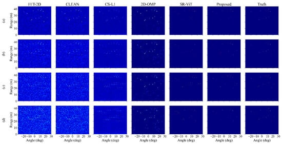
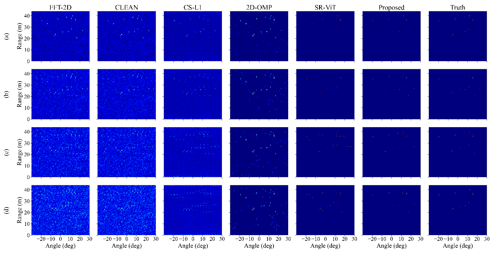
In the simulations, $T_p$ is set to 100 μs, and J takes integer values from 0 to 12. According to Equation (18), $v=(MN+J)d/\left(2T_p\right)$, corresponding to platform velocities of 78–195 m/s and virtual-array sparsities of 0–60%. Figure 3 presents the range–azimuth images at $\mathrm{SNR}=-10$ dB for $J=0,4,8,12$.

Figure 3. MIMO-SAR imaging results under different numbers of missing virtual elements J, $\mathrm{SNR}=-10$ dB. (a) $J=0$, (b) $J=4$, (c) $J=8$, (d) $J=12$.

The columns in Figure 3 show 2D-FFT [36], CLEAN [37], CS-$L_1$ [27], 2D-OMP [38], SR-ViT [39], SSTU, and the ground truth. All methods use the same data, radar parameters, and test samples. The conventional methods take complex time-domain echoes as input, whereas SR-ViT and SSTU receive their real and imaginary parts as two raw input channels. Within SSTU, the 2D-FFT layer converts these inputs into the three-channel spectral representation in Equation (26), comprising real, imaginary, and magnitude components.

For the conventional methods, the CLEAN gain is 0.1, the maximum atom number and relative residual threshold of 2D-OMP are 64 and ${10}^{-1}$, and the CS-L₁ regularization coefficient is 0.01. Each learning-based method uses its best-performing trained model. The loss weights are ${\beta }_w=1.0$, ${\beta }_d=0.5$, and ${\beta }_e=0.5$; the foreground threshold ratio and weighting factor are $\zeta =0.1$ and $\eta =50$, respectively. The difficult-pixel set ${\Omega }_e$ contains the 3% of pixels with the largest absolute errors.

Overall, as J increases, the number of azimuth ambiguities increases and the ambiguous responses become denser, with evident false-peak energy spreading and blurred target scatterers.

Under the full-aperture or mildly sparse cases ($J=0$ and $J=4$), 2D-FFT and CS-$L_1$ can recover the targets to some extent, but their images are still affected by noise. As J further increases, many false targets appear around the true targets, and effective imaging can no longer be achieved. CLEAN and 2D-OMP have stronger sparse-reconstruction capability. When J increases to 8, both methods can still recover the true targets, but obvious false-peak enhancement and mainlobe-energy weakening appear, and CLEAN also shows weak noise-suppression ability. When J increases to 12, CLEAN and 2D-OMP also fail to provide effective ambiguity suppression. In contrast, the proposed SSTU remains robust over the tested J range. Its background noise is significantly lower than that of the conventional methods, the target scattering points are clear, and no obvious false peaks are observed. Even under the severe case of $\mathrm{SNR}=-10$ dB and $J=12$, SSTU still accurately recovers the target spatial distribution, and the imaging quality is only weakly affected by aperture missing. These results show that SSTU can learn the imaging prior under sparse apertures and achieve robust multi-target imaging in low-SNR and highly sparse-aperture scenes.

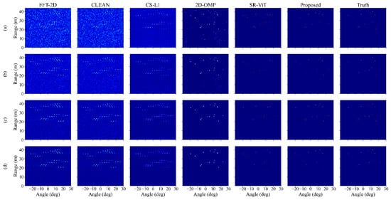
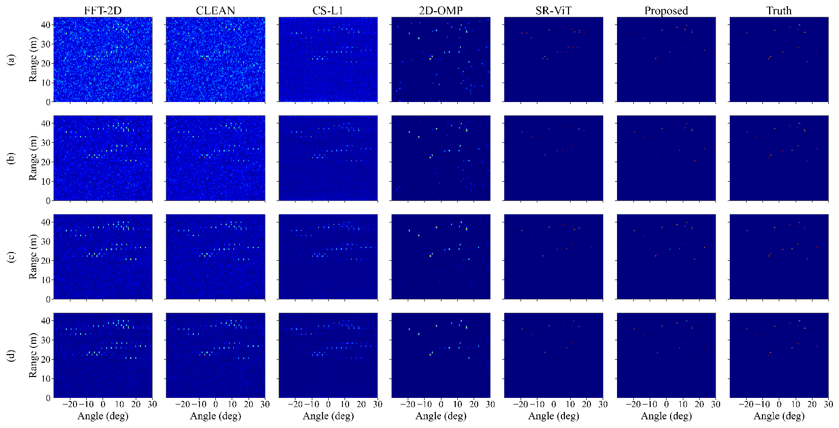
Figure 4 compares the imaging results of the six methods under different SNRs when $J=12$. As the SNR increases, all methods improve to some extent, but their sensitivities to noise differ substantially. At $\mathrm{SNR}=5$ dB, the influence of noise on image quality is relatively weak. However, 2D-FFT and CS-$L_1$ still produce strong azimuth ambiguities that are difficult to distinguish from true targets. CLEAN, 2D-OMP, and SR-ViT provide stronger ambiguity suppression than 2D-FFT and CS-$L_1$, but they still contain different levels of background noise, weak false peaks, and weakened mainlobe energy. In this case, target-detection or other post-processing methods may still identify the true targets, but more stringent extraction criteria are required. As the SNR decreases, the ambiguity-suppression capability of these three methods weakens further and target extraction becomes more difficult. In contrast, SSTU maintains the most stable reconstruction and remains closest to the ground truth under all tested SNR conditions, further confirming the conclusion drawn from Figure 3.

Figure 4. MIMO-SAR imaging results under different SNRs with the number of missing virtual elements fixed at $J=12$. (a) $\mathrm{SNR}=-10$ dB, (b) $\mathrm{SNR}=-5$ dB, (c) $\mathrm{SNR}=0$ dB, (d) $\mathrm{SNR}=5$ dB.

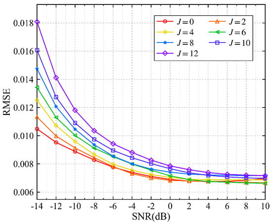
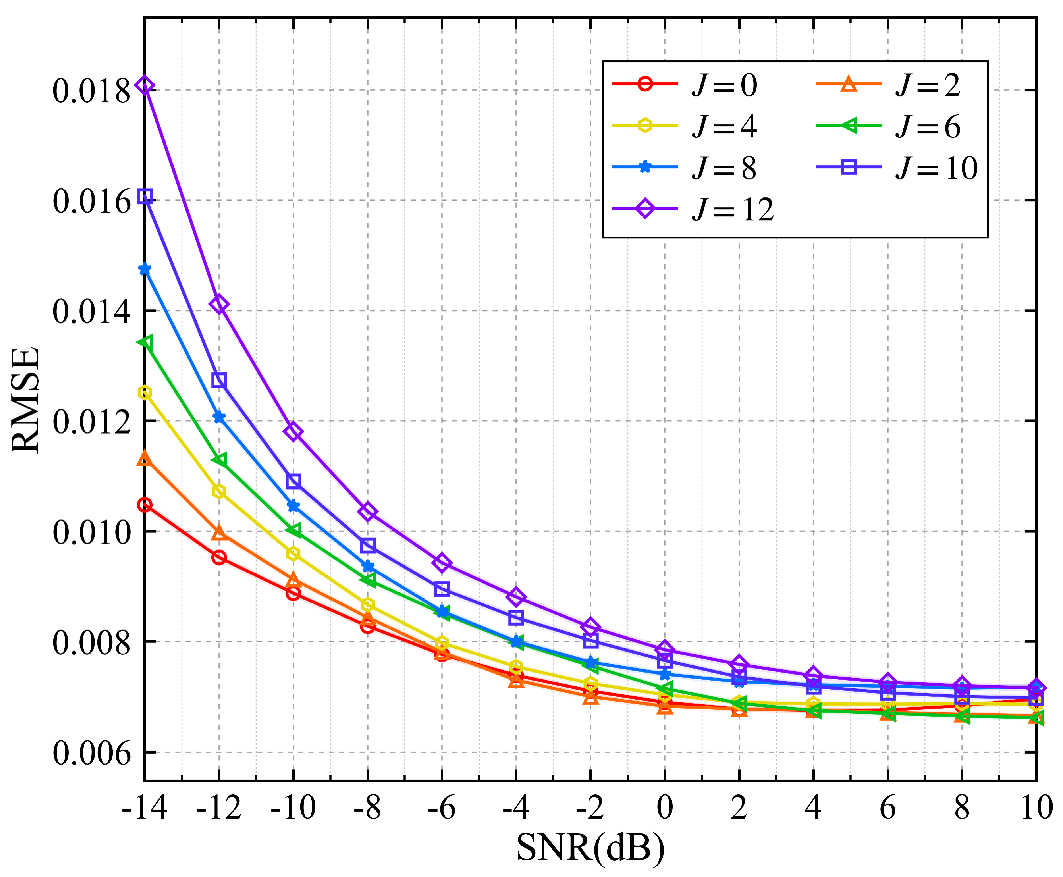
To further evaluate the image reconstruction accuracy of the proposed imaging method, Figure 5 compares the RMSE between the reconstructed image and the ground truth under different numbers of missing virtual elements J and different SNRs. As shown in the figure, the RMSE curves decrease as the SNR increases and gradually become saturated in the high-SNR region, indicating that reducing the noise level effectively improves reconstruction quality. As J increases, the spatial undersampling caused by the sparse aperture strengthens grating lobe interference, so the RMSE increases overall, especially in the low-SNR region. When the SNR increases to above $-6$ dB, the gaps among different curves become significantly smaller, and the RMSE falls below ${10}^{-2}$, demonstrating the effectiveness of the proposed algorithm in azimuth ambiguity suppression and high-resolution imaging.

Figure 5. Image RMSE variation with SNR under different numbers of missing virtual elements J.

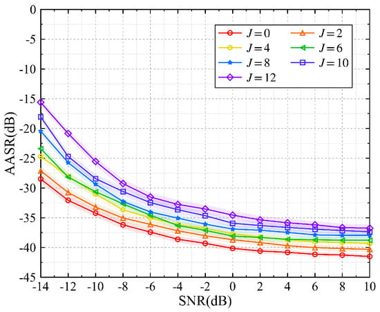
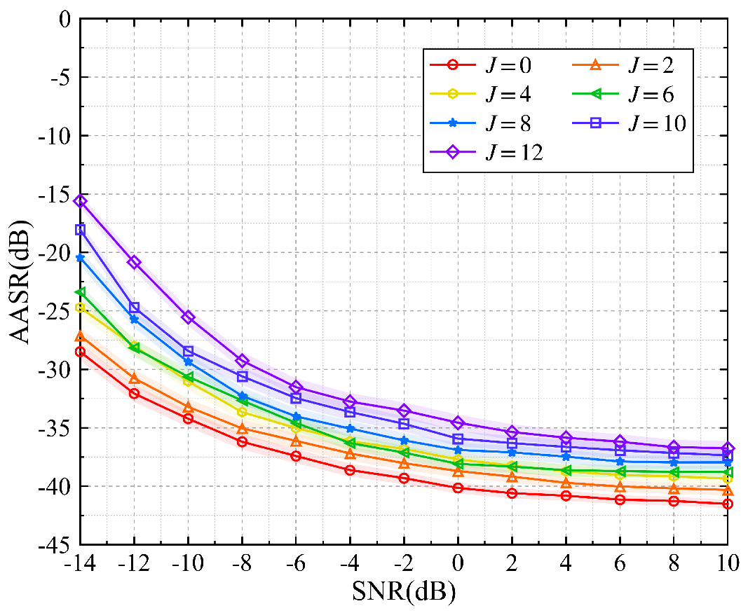
Figure 6 shows the variation of the azimuth ambiguity suppression ratio (AASR) of SSTU with SNR under different aperture-missing conditions ($J=0,2,4,6,8,10,12$), where the shaded regions indicate the corresponding error bands. In the range–azimuth image, for the sth target, let ${\Omega }_s$ be its mainlobe window, ${\Omega }_m={\bigcup }_{s=1}^S{\Omega }_s$ be the union of all mainlobe regions, and ${\Omega }_a$ be the union of azimuth ambiguity regions. Let $P_m$ and $P_a$ denote the total powers in the mainlobe and azimuth-ambiguity regions, respectively:

$$\begin{array}{cc}\hfill P_m& =\sum _{(r_{\mu },{\theta }_{\nu })\in {\Omega }_m}\mathcal{I}(r_{\mu },{\theta }_{\nu }),\hfill \\ \hfill P_a& =\sum _{(r_{\mu },{\theta }_{\nu })\in {\Omega }_a}\mathcal{I}(r_{\mu },{\theta }_{\nu }),\hfill \end{array}$$

(43)

where $\mathcal{I}(r_{\mu },{\theta }_{\nu })$ denotes the imaging power at the range–azimuth grid point $(r_{\mu },{\theta }_{\nu })$. The AASR is defined as [40]

$$\mathrm{AASR}=10{\log }_{10}\left({\displaystyle \frac{P_a}{P_m}}\right).$$

(44)

Figure 6. Average AASR of SSTU under different numbers of missing virtual elements J as the SNR changes.

The AASR measures the energy ratio between ambiguous responses and target mainlobes and is used to evaluate azimuth focusing quality. In the experiments, each mainlobe window is a fixed rectangle centered at the true target location and sized to cover the mainlobe response; the range and azimuth widths are set to 3 and 1 grid cells, respectively. The region outside the union of these windows is treated as the ambiguity region. The results show that SSTU is robust to both noise and sparse sampling. When $J=0$ and $J=4$, the AASR remains at a relatively low level. As the aperture gap becomes larger, such as for the $J=8$ and $J=12$ curves in the figure, the AASR increases at low SNR ($\mathrm{SNR}<-6$ dB) but rapidly converges below $-30$ dB as the SNR increases, showing the network’s effective compensation capability for sparse-aperture imaging.

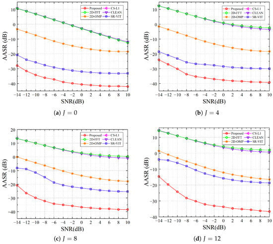
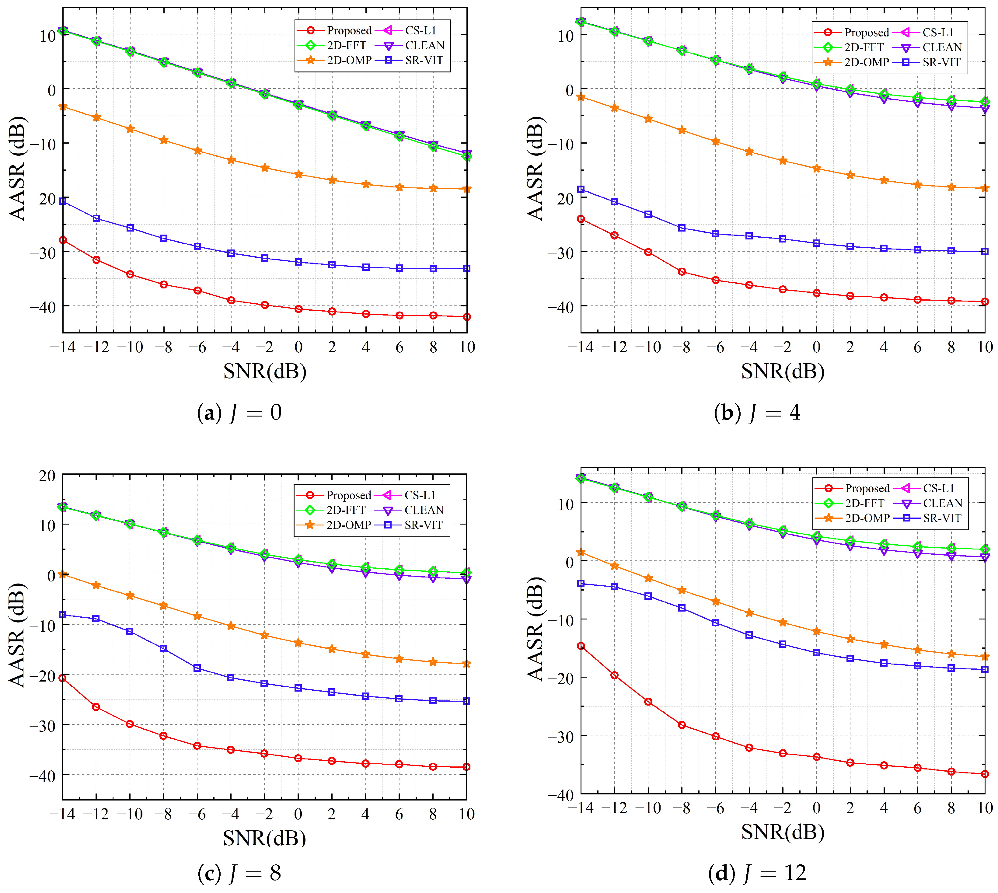
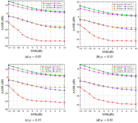
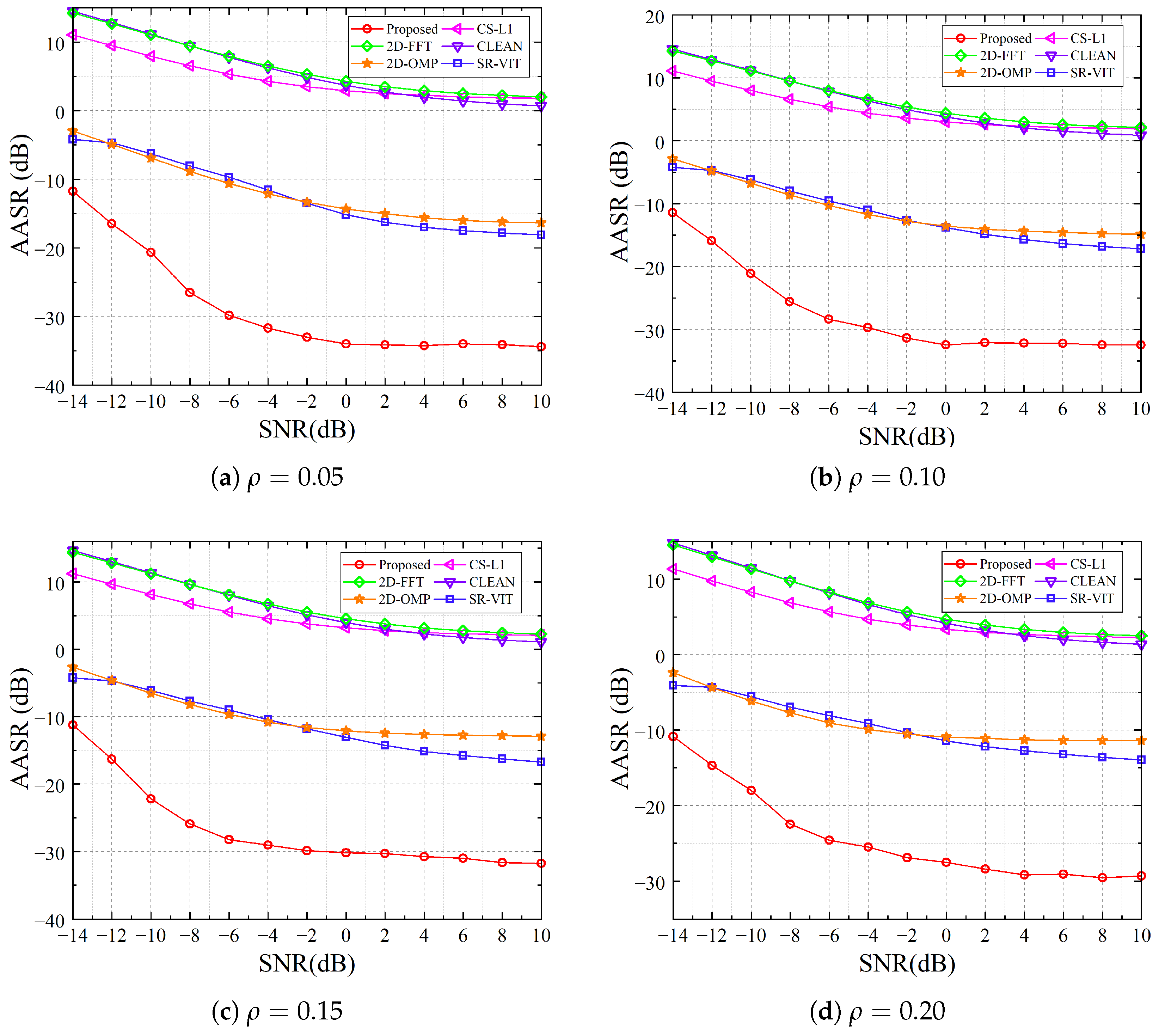
Figure 7 further compares SSTU with 2D-FFT, 2D-OMP, CS-$L_1$, CLEAN, and SR-ViT in terms of AASR variation with SNR. The 2D-FFT, CS-$L_1$, and CLEAN methods are sensitive to noise and sparse sampling, and their AASR values remain relatively high. 2D-OMP improves the result under some conditions, but its stability at low SNR is still limited. SR-ViT achieves lower AASR than the conventional methods, but its performance still degrades under high-sparsity conditions; when $J=12$, its performance decreases to a level comparable to 2D-OMP. In contrast, SSTU maintains lower AASR over the studied sparsity and SNR ranges, especially in the medium- and high-SNR regions, indicating stronger noise and ambiguity suppression capability in sparse MIMO-SAR imaging.

Figure 7. Comparison of average AASR variation with SNR for different methods under different numbers of missing virtual elements J. The compared methods are 2D-FFT [36], CS-$L_1$ [27], CLEAN [37], 2D-OMP [38], SR-ViT [39], and SSTU.

Table 3 lists the SSIM values under different sparsities and SNRs. Together with Figure 3 and Figure 4, the results show that in the sparse imaging task, true targets occupy only a small image area, whereas sparse apertures introduce strong periodic azimuth ambiguities. The conventional 2D-FFT, CLEAN, and CS-$L_1$ methods provide limited suppression of azimuth ambiguity and noise; under high sparsity and low SNR, they produce numerous background false peaks and diffuse sidelobes, leading to rapid structural-similarity degradation and low SSIM values. 2D-OMP exploits sparsity to suppress most noise and raises the SSIM above 0.95, but its grating lobe suppression weakens as the number of missing virtual elements J increases. At higher SNRs, the SSIM of conventional methods improves, but azimuth ambiguity remains insufficiently resolved.

Table 3. SSIM comparison of different methods with varying J.

SNR	Method	$\mathit{J}=0$	$\mathit{J}=4$	$\mathit{J}=8$	$\mathit{J}=12$
$-5$ dB	2D-FFT [36]	0.078	0.051	0.040	0.033
	CS-$L_1$ [27]	0.077	0.072	0.072	0.069
	CLEAN [37]	0.080	0.052	0.042	0.034
	2D-OMP [38]	0.954	0.954	0.953	0.952
	SR-ViT [39]	0.997	0.997	0.995	0.980
	SSTU	0.998	0.998	0.998	0.998
5 dB	2D-FFT [36]	0.440	0.306	0.254	0.202
	CS-$L_1$ [27]	0.441	0.384	0.381	0.350
	CLEAN [37]	0.444	0.311	0.258	0.207
	2D-OMP [38]	0.977	0.977	0.977	0.975
	SR-ViT [39]	0.997	0.997	0.996	0.995
	SSTU	0.999	0.999	0.999	0.998

In contrast, deep-learning-based methods learn structural differences among targets, grating lobes, and noise from training data, thereby suppressing noise and background false peaks while recovering target regions. SR-ViT degrades with increasing sparsity; although its SSIM decreases only slightly and remains high, this is because sparse images are dominated by background pixels, so even a small SSIM drop can correspond to noticeable performance degradation. The proposed SSTU maintains the highest SSIM over the studied sparsity range, demonstrating its structural reconstruction capability and robustness under sparse and noisy conditions.

To evaluate the local sidelobe suppression capability of different algorithms, Table 4 reports the peak sidelobe ratio (PSLR) and integrated sidelobe ratio (ISLR). To avoid divergence in logarithmic calculation, the noise floor is set to approximately $-46$ dB.

Table 4. PSLR/ISLR comparison of different methods with varying J.

SNR	Method	PSLR/ISLR (dB)
		$\mathit{J}=\mathbf{0}$	$\mathit{J}=\mathbf{4}$	$\mathit{J}=\mathbf{8}$	$\mathit{J}=\mathbf{12}$
$-5$ dB	2D-FFT [36]	−17.4/−3.7	−6.5/1.4	−3.1/3.6	−1.6/5.0
	CS-$L_1$ [27]	−17.4/−3.7	−8.5/0.1	−4.2/2.6	−2.1/3.9
	CLEAN [37]	−17.4/−3.9	−8.0/0.4	−4.9/2.4	−3.2/3.8
	2D-OMP [38]	−28.6/−28.3	−25.6/−25.2	−23.1/−22.7	−21.0/−20.5
	SR-ViT [39]	−45.7/−45.7	−45.5/−45.6	−42.3/−42.3	−34.1/−41.1
	SSTU	−45.5/−45.5	−45.5/−45.6	−45.4/−45.7	−45.0/−45.0
5 dB	2D-FFT [36]	−26.9/−13.4	−6.8/−1.0	−3.1/1.8	−1.6/3.5
	CS-$L_1$ [27]	−26.9/−13.4	−9.2/−3.2	−4.7/0.4	−2.3/2.0
	CLEAN [37]	−26.9/−13.7	−8.5/−2.6	−5.3/0.2	−3.4/1.9
	2D-OMP [38]	−35.1/−34.7	−33.6/−33.2	−32.2/−31.9	−28.6/−28.2
	SR-ViT [39]	−45.7/−45.7	−45.3/−45.4	−43.3/−43.6	−40.9/−41.1
	SSTU	−45.5/−45.5	−45.6/−45.6	−45.7/−45.7	−45.4/−45.4

As shown in Table 4, the three categories of methods exhibit different sidelobe degradation patterns. For 2D-FFT, CLEAN, and CS-$L_1$, both PSLR and ISLR deteriorate as J increases, with a larger degradation in ISLR; under high sparsity, ISLR even becomes positive, indicating that sparse-aperture-induced energy leakage is distributed diffusely rather than appearing as isolated sidelobe peaks. This trend persists at $\mathrm{SNR}=5$ dB, showing that such sidelobe enhancement cannot be removed simply by improving the SNR. The output of 2D-OMP is a sparse point estimate, so its PSLR and ISLR values are close and are overall lower than those of the preceding methods, but they still degrade by about 8 dB as J increases. The learning-based methods show significantly lower sidelobe levels: SR-ViT is comparable to SSTU when $J<4$, but also degrades as J increases; SSTU remains at approximately the $-45$ dB level under both SNR settings and all J values. These results indicate that SSTU not only suppresses azimuth ambiguity but also maintains a low sidelobe level.

3.2. Measured-Data Results

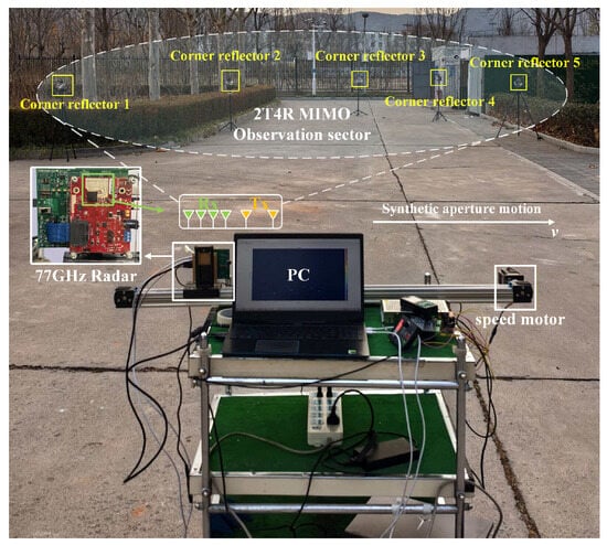
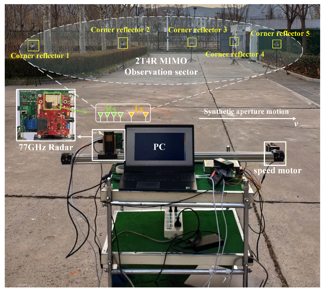
To validate the effectiveness of the proposed method on measured data, an outdoor open-area experiment was conducted. The experimental scenario is shown in Figure 8. The experiment used a 77 GHz industrial millimeter-wave radar sensor produced by Texas Instruments (IWR1443 with DCA1000EVM). The radar was mounted on a linear rail and driven by a speed-controlled motor along the array direction. The radar was configured in a two-transmitter four-receiver TDM-MIMO mode. Each MIMO snapshot consisted of two consecutive TDM chirps and formed eight virtual elements. In the measured imaging experiment, 32 rail positions were selected, yielding 256 equivalent azimuth samples and an effective synthetic-aperture length of approximately 0.50 m. The detailed experimental parameters are listed in Table 5.

Figure 8. Outdoor experiment scenario for MIMO-SAR imaging.

Table 5. Measured-data experimental parameters.

Parameter	Notation	Default Value
Wavelength	$\lambda$	0.0039 m
Number of transmit antennas	M	2
Number of receive antennas	N	4
Transmit bandwidth	B	3186.45 MHz
Chirp slope	K	63.73 MHz/μs
Chirp period	$T_c$	50 μs
Slow-time sampling interval	$T_p$	10 ms
Sampling rate	$f_s$	37.5 Msps
Fast-time samples	$N_s$	256
MIMO snapshots	L	32
Synthetic-aperture length	–	0.5 m
Rail length	–	1 m
Motor velocity	v	0.78 m/s

The imaging scene contains five fixed targets formed by corner reflectors at different ranges and azimuth angles. The radar moved uniformly along the rail direction to acquire MIMO-SAR echoes. Different slow-time sampling displacements were obtained by uniform subsampling, with $J=0,4,8,12$, consistent with the simulation settings. Figure 9 shows the imaging results of different algorithms for the above scene.

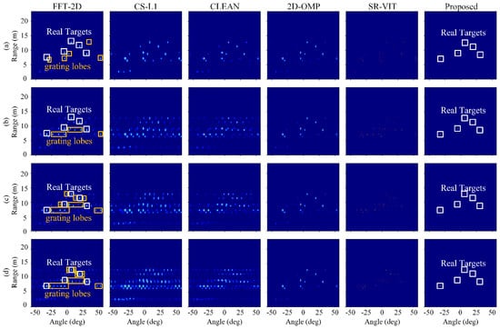
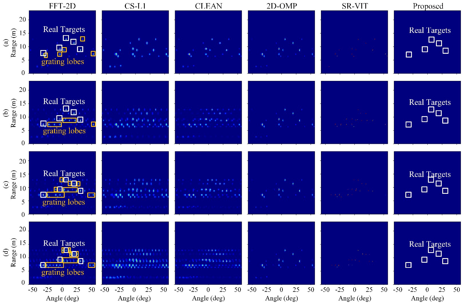
Figure 9. Measured-data imaging results under different numbers of missing virtual elements J. (a) $J=0$, (b) $J=4$, (c) $J=8$, (d) $J=12$.

When $J=0$, although no additional aperture missing is artificially introduced, the nonideal rail motion can still cause equivalent sampling deviations, resulting in false peaks and sidelobe leakage in the range–azimuth images, as indicated by the yellow boxes in Figure 9. The compared algorithms show limited generalization capability and insufficient suppression of nonideal responses caused by actual motion errors. As the slow-time sampling displacement increases, periodic undersampling of the effective aperture becomes more severe, and typical grating lobes appear in the angular dimension. When $J=8$, nearly symmetric false peaks with comparable energy appear on both sides of the true peaks, making it difficult for conventional amplitude-threshold or fixed-sidelobe-threshold detection strategies to distinguish true scatterers from false peaks. SR-ViT can suppress most low-energy grating lobes, but residual responses still remain under the joint influence of strong grating lobes and measured motion errors. In contrast, after SSTU reconstruction, false peaks and grating lobes are significantly weakened. The five strong scatterers consistent with the scene become more concentrated, and stray energy is suppressed.

In addition, Table 6 compares the AASR values of different methods in the measured experiment. Because measured data are prone to azimuth ambiguities even under full-aperture conditions, the AASR values of the compared methods are already high at $J=0$ and further deteriorate as J increases. For SR-ViT, although most grating lobes are suppressed, the remaining grating lobe responses are still relatively strong, resulting in high AASR values and indicating that its generalization is strongly affected by real experimental conditions. In contrast, the proposed method produces no obvious ambiguities in the reconstructed images, and its AASR remains below $-40$ dB.

Table 6. AASR comparison of different methods in measured experiments.

Method	AASR (dB)
	$\mathit{J}=\mathbf{0}$	$\mathit{J}=\mathbf{4}$	$\mathit{J}=\mathbf{8}$	$\mathit{J}=\mathbf{12}$
2D-FFT	−2.81	1.07	3.04	4.47
CS-$L_1$	−2.88	1.01	3.03	4.39
CLEAN	2.45	4.95	6.32	7.65
2D-OMP	−3.00	−3.02	−2.85	−2.89
SR-ViT	1.03	2.30	3.32	1.68
SSTU	<$-40$	<$-40$	<$-40$	<$-40$

4. Discussion

4.1. Ablation Analysis

Table 7a evaluates the contribution of each network component. To provide a purely conventional reference, a 2D-FFT+CFAR baseline is first introduced, where constant false alarm rate (CFAR) detection is applied to the 2D-FFT image and pixels that do not pass the detection threshold are set to zero [41]. The guard-cell half-width, training-cell half-width, and false-alarm probability are set to 2, 8, and ${10}^{-3}$, respectively. The baseline model uses the 2D-FFT layer spectral-prior front end, a U-Net encoder–decoder, and the standard $L_1$ loss. The w/o 2D-FFT layer variant removes the 2D-FFT layer from the full network and directly uses raw echo features as input. The w/o Swin variant removes the Swin Transformer module and keeps only the U-Net structure with the sparse compound loss. The w/o sparse loss variant keeps the 2D-FFT layer and Swin Transformer but replaces the sparse compound loss with the standard $L_1$ loss. The full model denotes the complete SSTU network.

Table 7. Ablation results under different numbers of missing virtual elements J.

(a) Ablation of network components.
Variant	Network component			AASR (dB)
	2D-FFT Layer	Swin	Sparse loss	$J=0$	$J=4$	$J=8$	$J=12$
2D-FFT+CFAR	–	–	–	−19.87	−4.61	−0.92	0.76
Baseline	✔	–	–	−36.25	−33.17	−31.54	−28.92
w/o 2D-FFT Layer	–	✔	✔	N/A	N/A	N/A	N/A
w/o Swin	✔	–	✔	−36.48	−33.62	−32.41	−29.17
w/o Sparse Loss	✔	✔	–	−34.08	−31.72	−30.30	−27.58
Full	✔	✔	✔	−37.99	−35.09	−33.54	−31.01
(b) Ablation of the 2D-FFT Layer output channels.
Variant	2D-FFT Layer output channel			AASR (dB)
	$\mathrm{Re}\left(\mathbf{A}\right)$	$\mathrm{Im}\left(\mathbf{A}\right)$	$\left|\mathbf{A}\right|$	$J=0$	$J=4$	$J=8$	$J=12$
w/o Magnitude	✔	✔	–	−36.54	−34.36	−31.99	−30.11
w/o Real and Imaginary	–	–	✔	−35.70	−31.99	−31.24	−27.19
Full	✔	✔	✔	−37.99	−35.09	−33.54	−31.01

N/A indicates that the validation loss did not converge stably during training; therefore, no reliable AASR value was obtained.

The component ablation results in Table 7a show that simple 2D-FFT threshold postprocessing cannot effectively suppress the strong sidelobes and periodic grating lobes caused by sparse apertures; its AASR is much higher than those of all learning-based variants, indicating that conventional amplitude-threshold methods fail in this task. The w/o 2D-FFT layer variant does not converge stably, since the network must infer the target heatmap directly from raw complex echoes. Without the 2D-FFT layer, range compression, azimuth focusing, sparse-aperture compensation, and grating-lobe suppression are all left to the network, making the optimization substantially harder. This indicates that the spectral prior provided by the 2D-FFT layer is a key front end for learning the sparse-aperture degradation compensation mapping.

With the 2D-FFT layer fixed, w/o Swin achieves lower AASR than the baseline for all J, showing that the sparse compound loss improves the network’s focus on target mainlobes and residual ambiguous responses. After the Swin Transformer is further introduced, the full model obtains the lowest AASR under all aperture-missing conditions, especially reducing the AASR from −29.17 dB to −31.01 dB at $J=12$ compared with w/o Swin. In contrast, w/o sparse loss degrades for all J, suggesting that long-range correlation modeling should be guided by target-region weighting and sparse-prior constraints to avoid jointly aggregating mainlobe and grating lobe responses. These results verify the complementarity among the 2D-FFT layer, Swin Transformer, and sparse compound loss.

Table 7b further evaluates the three spectral channels generated by the 2D-FFT layer. As defined in Equation (26), its output is $\mathbf{X}=\left[\mathrm{Re}\right(\mathbf{A}),\mathrm{Im}(\mathbf{A}),|\mathbf{A}\left|\right]$. The full configuration retains all three channels, w/o magnitude removes $\left|\mathbf{A}\right|$, and w/o real and imaginary removes $\mathrm{Re}\left(\mathbf{A}\right)$ and $\mathrm{Im}\left(\mathbf{A}\right)$.

Table 7b shows that removing the magnitude channel increases the average AASR by approximately 1.16 dB. Removing the real and imaginary channels increases the average AASR by approximately 2.88 dB and causes a 3.82 dB degradation at $J=12$. Overall, the full three-channel representation achieves the lowest AASR for all J. These results suggest that the real-imaginary and magnitude representations provide complementary information and that their joint use is more effective than either reduced configuration under the tested conditions.

4.2. Robustness to Position Errors

Because platform motion and synchronization errors in practical systems may cause sampling positions to deviate from their ideal positions, the influence of platform position errors on imaging quality and sidelobe suppression is further examined under a high-sparsity condition ($J=12$), as shown in Figure 10. The position-jitter strength is represented by the normalized parameter $\rho ={\sigma }_y/d$, where ${\sigma }_y$ is the standard deviation of the sampling position. It should be noted that position jitter is introduced only during testing to evaluate the model’s robustness to unseen aperture-position errors.

Figure 10. Comparison of average AASR variation with SNR for different methods under different position errors $\rho$. The compared methods are 2D-FFT [36], CS-$L_1$ [27], CLEAN [37], 2D-OMP [38], SR-ViT [39], and SSTU.

As $\rho$ increases, the actual sampling positions gradually deviate from the ideal equivalent-aperture geometry, and echo phase errors accumulate. Consequently, all methods exhibit increased sidelobes and enhanced grating lobes. This degradation shows a clear two-stage behavior. For small position errors ($\rho \le 0.1$), the AASR of each method increases only slightly relative to the error-free case, and the imaging degradation is still dominated by sparse sampling and noise. As $\rho$ further increases, random phase errors scatter part of the mainlobe energy into the background, causing the AASR to rise more rapidly. At large $\rho$, the improvement brought by increasing SNR tends to saturate, and geometric mismatch becomes the dominant error source.

Different methods also show different sensitivities to $\rho$. For 2D-FFT, CLEAN, and CS-$L_1$, the metrics vary relatively slowly because their grating lobe energy is already high under strong undersampling, so the additional noise floor induced by position errors is masked by the existing degradation. By contrast, 2D-OMP, SR-ViT, and the proposed method have lower baseline sidelobe levels, making the effect of geometric mismatch more evident. Although the proposed method also degrades under large position errors and its advantage over the competing methods narrows, it consistently maintains the lowest AASR over all SNR and $\rho$ conditions. This indicates that the learned spectral prior is more robust to position errors and can more effectively suppress imaging degradation jointly caused by undersampling, noise, and motion errors.

4.3. Computational Efficiency

Table 8 summarizes the quantitative evaluation of the computational complexity and inference efficiency of the SSTU network. The model was trained and evaluated on an NVIDIA RTX 5090 platform. It contains 0.745 M parameters, requires 15.751 GFLOPs per frame, and achieves an average single-frame inference latency of 3.262 ms, corresponding to 306.6 frames per second. The FLOPs of SSTU mainly come from multiscale feature fusion and progressive upsampling in the decoder, whereas the actual inference time is primarily affected by window self-attention in the Swin Transformer bottleneck. Overall, SSTU achieves a favorable balance between imaging performance and computational efficiency and has potential for deployment on embedded hardware.

Table 8. Computational efficiency of SSTU.

Component	Parameters (M)	FLOPs (G)	Latency (ms)
2D-FFT layer	0.000	0.000	0.122
CNN encoder	0.072	1.283	0.213
Swin Transformer bottleneck	0.313	0.416	2.258
Decoder	0.360	14.043	0.517
Output head	0.000	0.008	0.028
Runtime overhead	0.000	0.001	0.124
Total model	0.745	15.751	3.262

4.4. Applicability and Limitations

In the TDM-MIMO SAR scenario considered in this work, the $MN$ consecutive virtual phase centers within each MIMO snapshot, together with the missing virtual elements between adjacent groups, form a block-sparse virtual aperture. This aperture structure determines the spectral relationship among the mainlobes, sidelobes, and periodic grating lobes. Since SSTU builds both its input representation and spectral prior on this aperture structure, the proposed method is primarily intended for azimuth ambiguity suppression in TDM-MIMO SAR with sparse virtual apertures. Nevertheless, the same idea may be extendable to other sparse-aperture imaging problems that exhibit stable spectral-domain degradation patterns, such as single-channel SAR and sparse-aperture ISAR. Practical use in these scenarios, however, would require task-specific adaptation to the corresponding imaging geometry and training data.

The above results show that the proposed SSTU-based MIMO-SAR imaging method has better ambiguity suppression capability and imaging stability under aperture sparsity and motion nonidealities. In addition, because the network is trained mainly on sparse-aperture degradation samples generated from simulated data and no dedicated fine-tuning is performed on the field data, the proposed method still maintains effective grating lobe suppression and target focusing on measured data. This result provides preliminary evidence of the simulation-to-measurement transfer capability of the proposed method.

It should be noted that the measured experiment constructs the sparse moving-array condition studied in this paper through a low-speed rail and spatial-position subsampling. This verifies reconstruction effectiveness on nonideal measured radar data, but does not include high-dynamic error factors such as intra-group motion, nonuniform motion, and attitude disturbance. The performance of the method under practical complex motion conditions, such as airborne and vehicle-mounted platforms, therefore requires further validation through field experiments.

5. Conclusions

This paper proposed an SSTU-network-based sparse moving-array imaging method for millimeter-wave FMCW MIMO-SAR, addressing azimuth spectral aliasing, periodic grating lobe enhancement, and image-quality degradation caused by slow-time aperture undersampling under low-SNR conditions. The method realizes range–azimuth image reconstruction under sparse moving apertures by combining 2D-FFT-based spectral guidance with local–global feature fusion. Simulations under different aperture sparsities and SNRs verify its imaging robustness against the coupled degradation caused by strong aperture undersampling and noise. The results show that when the aperture sparsity reaches 60% and the SNR is higher than $-6$ dB, the proposed method can still stably recover the range–azimuth distribution of multiple point targets, with an azimuth ambiguity suppression ratio better than −30 dB, outperforming the compared methods. The single-frame inference latency is 3.262 ms, indicating good real-time imaging capability. Further 77 GHz radar field experiments are conducted using a two-transmitter four-receiver MIMO array and five outdoor corner reflectors. The results show that the proposed method effectively suppresses azimuth grating lobes and background stray responses under 60% sparse moving-aperture sampling while preserving a clear distribution of the dominant scatterers.

This study verifies the effectiveness of the SSTU-based sparse-aperture imaging framework through relatively comprehensive simulations and target-imaging experiments using data acquired by an actual radar platform. Future work will further consider method generalization under complex extended targets, nonideal motion errors, and cluttered backgrounds and will explore lightweight deployment on embedded radar platforms.

References

- Moreira, A.; Prats-Iraola, P.; Younis, M.; Krieger, G.; Hajnsek, I.; Papathanassiou, K.P. A tutorial on synthetic aperture radar. IEEE Geosci. Remote Sens. Mag. 2013, 1, 6–43. [Google Scholar] [CrossRef] [Scilit]
- Bekar, A.; Antoniou, M.; Baker, C.J. Low-Cost, High-Resolution, Drone-Borne SAR Imaging. IEEE Trans. Geosci. Remote Sens. 2022, 60, 5208811. [Google Scholar] [CrossRef] [Scilit]
- Hasch, J.; Topak, E.; Schnabel, R.; Zwick, T.; Weigel, R.; Waldschmidt, C. Millimeter-Wave Technology for Automotive Radar Sensors in the 77 GHz Frequency Band. IEEE Trans. Microw. Theory Tech. 2012, 60, 845–860. [Google Scholar] [CrossRef] [Scilit]
- Patole, S.M.; Torlak, M.; Wang, D.; Ali, M. Automotive radars: A review of signal processing techniques. IEEE Signal Process. Mag. 2017, 34, 22–35. [Google Scholar] [CrossRef] [Scilit]
- Chen, S.; Liu, M.; Lu, F.; Xing, M. A Target Identification Method for the Millimeter Wave Seeker via Correlation Matching and Beam Pointing. Sensors 2019, 19, 2530. [Google Scholar] [CrossRef] [Scilit] [PubMed]
- Pirkani, A.; Stove, A.G.; Kumar, D.; Cherniakov, M.; Gashinova, M.S. 77 GHz FMCW Imaging Radar for Low Observable and Small Marine Target Detection in Dynamic Sea Conditions Based on Combined MIMO and DBS. IEEE Trans. Radar Syst. 2024, 2, 517–534. [Google Scholar] [CrossRef] [Scilit]
- Hamidi, S. 3D Near-Field Virtual MIMO-SAR Imaging Using FMCW Radar Systems at 77 GHz. In Proceedings of the 2024 IEEE Canadian Conference on Electrical and Computer Engineering (CCECE), Kingston, ON, Canada, 6–9 August 2024; pp. 264–270. [Google Scholar] [CrossRef] [Scilit]
- Krieger, G. MIMO-SAR: Opportunities and Pitfalls. IEEE Trans. Geosci. Remote Sens. 2014, 52, 2628–2645. [Google Scholar] [CrossRef] [Scilit]
- Gao, X.; Roy, S.; Xing, G. MIMO-SAR: A Hierarchical High-Resolution Imaging Algorithm for mmWave FMCW Radar in Autonomous Driving. IEEE Trans. Veh. Technol. 2021, 70, 7322–7334. [Google Scholar] [CrossRef] [Scilit]
- Han, Y.; Yan, X.; Gao, X.; Yi, G.; Dai, J. Fuze Target Recognition Method Based on Motion Array Microwave Imaging and Multi-Scale Deformable Convolutional Network. Binggong Xuebao/Acta Armamentarii 2025, 46, 214–224. [Google Scholar]
- Niu, S.; Jin, G.; Cheng, Y.; Wang, Y.; Zhang, H.; Zhu, D. A Novel MIMO SAR Transmission Scheme for Restoring Repeated Equivalent Phase Centers. IEEE Trans. Geosci. Remote Sens. 2023, 61, 5216618. [Google Scholar] [CrossRef] [Scilit]
- Tebaldini, S.; Manzoni, M.; Ferro-Famil, L.; Banda, F.; Giudici, D. Minimum Redundancy Wavenumber Illumination for FDM MIMO spaceborne SAR Tomography. In Proceedings of the 2024 International Radar Conference (RADAR), Rennes, France, 21–25 October 2024; pp. 1–6. [Google Scholar] [CrossRef] [Scilit]
- Wang, S.; Li, S.; Hoorfar, A.; Miao, K.; Zhao, G.; Sun, H. Compressive Sensing-Based Sparse MIMO Array Synthesis for Wideband Near-Field Millimeter-Wave Imaging. IEEE Trans. Aerosp. Electron. Syst. 2023, 59, 7681–7697. [Google Scholar] [CrossRef] [Scilit]
- Wang, S.; Li, S.; Ren, B.; Miao, K.; Zhao, G.; Sun, H. Convex Optimization-Based Design of Sparse Arrays for 3-D Near-Field Imaging. IEEE Sens. J. 2023, 23, 9640–9648. [Google Scholar] [CrossRef] [Scilit]
- Zhao, H.; Zhang, Z.; Chen, Z.; Fan, H.; Lv, Z.; Bi, J. A Multiple-Input Multiple-Output Synthetic Aperture Radar Echo Separation and Range Ambiguity Suppression Processing Framework for High-Resolution Wide-Swath Imaging. Remote Sens. 2025, 17, 609. [Google Scholar] [CrossRef] [Scilit]
- Xue, B.; Zhang, G.; Gini, F.; Greco, M.S.; Leung, H. Range Resolution Enhancement for Miniature Dechirped MMW MIMO-SAR. IEEE Trans. Geosci. Remote Sens. 2024, 62, 5210516. [Google Scholar] [CrossRef] [Scilit]
- Manzoni, M.; Tebaldini, S.; Monti-Guarnieri, A.V.; Prati, C.M.; Russo, I. A Comparison of Processing Schemes for Automotive MIMO SAR Imaging. Remote Sens. 2022, 14, 4696. [Google Scholar] [CrossRef] [Scilit]
- Zhang, B.; Xu, G.; Zhou, R.; Zhang, H.; Hong, W. Multi-Channel Back-Projection Algorithm for mmWave Automotive MIMO SAR Imaging with Doppler-Division Multiplexing. IEEE J. Sel. Top. Signal Process. 2023, 17, 445–457. [Google Scholar] [CrossRef] [Scilit]
- Tang, J.; Liu, Z.; Ran, L.; Xie, R.; Qin, J. Forward-Looking Super-Resolution Imaging of MIMO Radar via Sparse and Double Low-Rank Constraints. Remote Sens. 2023, 15, 609. [Google Scholar] [CrossRef] [Scilit]
- Han, Y.; Yan, X.; Wang, J.; Zheng, S.; Yu, H.; Dai, J. A sparse moving array imaging approach for FMCW radar with dual-aperture adaptive azimuth ambiguity suppression and adaptive QR decomposition. Def. Technol. 2025, 50, 254–271. [Google Scholar] [CrossRef] [Scilit]
- Cerutti-Maori, D.; Sikaneta, I.; Klare, J.; Gierull, C.H. MIMO SAR Processing for Multichannel High-Resolution Wide-Swath Radars. IEEE Trans. Geosci. Remote Sens. 2014, 52, 5034–5055. [Google Scholar] [CrossRef] [Scilit]
- Tang, X.; Yang, J.; Zhang, Y. Motion-Compensated Reconstruction for Azimuth Multi-Channel Synthetic Aperture Ladar: A Robust Framework for High-Resolution Wide-Swath Imaging. Remote Sens. 2026, 18, 1100. [Google Scholar] [CrossRef] [Scilit]
- Hu, X.; Ma, C.; Lu, X.; Yeo, T.S. Compressive Sensing SAR Imaging Algorithm for LFMCW Systems. IEEE Trans. Geosci. Remote Sens. 2021, 59, 8486–8500. [Google Scholar] [CrossRef] [Scilit]
- Focsa, A.; Anghel, A.; Datcu, M. A Compressive-Sensing Approach for Opportunistic Bistatic SAR Imaging Enhancement by Harnessing Sparse Multiaperture Data. IEEE Trans. Geosci. Remote Sens. 2022, 60, 5205914. [Google Scholar] [CrossRef] [Scilit]
- Li, S.; Zhao, G.; Li, H.; Ren, B.; Hu, W.; Liu, Y.; Yu, W.; Sun, H. Near-Field Radar Imaging via Compressive Sensing. IEEE Trans. Antennas Propag. 2015, 63, 828–833. [Google Scholar] [CrossRef] [Scilit]
- Miran, E.A.; Oktem, F.S.; Koc, S. Sparse Reconstruction for Near-Field MIMO Radar Imaging Using Fast Multipole Method. IEEE Access 2021, 9, 151578–151589. [Google Scholar] [CrossRef] [Scilit]
- Lee, S.; Jung, Y.; Lee, M.; Lee, W. Compressive Sensing-Based SAR Image Reconstruction from Sparse Radar Sensor Data Acquisition in Automotive FMCW Radar System. Sensors 2021, 21, 7283. [Google Scholar] [CrossRef] [Scilit] [PubMed]
- Wang, M.; Wei, S.; Liang, J.; Zeng, X.; Wang, C.; Shi, J.; Zhang, X. RMIST-Net: Joint Range Migration and Sparse Reconstruction Network for 3-D mmW Imaging. IEEE Trans. Geosci. Remote Sens. 2022, 60, 5205117. [Google Scholar] [CrossRef] [Scilit]
- Manisali, I.; Oral, O.; Oktem, F.S. Efficient physics-based learned reconstruction methods for real-time 3D near-field MIMO radar imaging. Digit. Signal Process. 2024, 144, 104274. [Google Scholar] [CrossRef] [Scilit]
- Ren, J.; Luo, Y.; Fan, C.; Feng, W.; Su, L.; Wang, H. RAU-Net-Based Imaging Method for Spatial-Variant Correction and Denoising in Multiple-Input Multiple-Output Radar. Remote Sens. 2024, 16, 80. [Google Scholar] [CrossRef] [Scilit]
- Dai, Y.; Jin, T.; Song, Y.; Sun, S.; Wu, C. Convolutional Neural Network with Spatial-Variant Convolution Kernel. Remote Sens. 2020, 12, 2811. [Google Scholar] [CrossRef] [Scilit]
- Liu, Z.; Lin, Y.; Cao, Y.; Hu, H.; Wei, Y.; Zhang, Z.; Lin, S.; Guo, B. Swin Transformer: Hierarchical Vision Transformer using Shifted Windows. In Proceedings of the 2021 IEEE/CVF International Conference on Computer Vision (ICCV), Montreal, QC, Canada, 11–17 October 2021; pp. 9992–10002. [Google Scholar] [CrossRef] [Scilit]
- Qi, X.; Zhang, Y.; Jiang, Y.; Liu, Z.; Yang, C. MosReformer: Reconstruction and Separation of Multiple Moving Targets for Staggered SAR Imaging. Remote Sens. 2023, 15, 4911. [Google Scholar] [CrossRef] [Scilit]
- Mao, Y.; He, G.; Wang, G.; Yin, R.; Peng, Y.; Guan, B. DESAT: A Distance-Enhanced Strip Attention Transformer for Remote Sensing Image Super-Resolution. Remote Sens. 2024, 16, 4251. [Google Scholar] [CrossRef] [Scilit]
- Ronneberger, O.; Fischer, P.; Brox, T. U-Net: Convolutional Networks for Biomedical Image Segmentation. In Medical Image Computing and Computer-Assisted Intervention—MICCAI 2015; Navab, N., Hornegger, J., Wells, W., Frangi, A., Eds.; Lecture Notes in Computer Science; Springer: Cham, Switzerland, 2015; Volume 9351. [Google Scholar] [CrossRef] [Scilit]
- Jardak, S.; Ahmed, S.; Alouini, M.-S. Low Complexity Moving Target Parameter Estimation for MIMO Radar Using 2D-FFT. IEEE Trans. Signal Process. 2017, 65, 4745–4755. [Google Scholar] [CrossRef] [Scilit]
- Polisano, M.G.; Manzoni, M.; Tebaldini, S.; Monti-Guarnieri, A.; Prati, C.M.; Russo, I. Very High Resolution Automotive SAR Imaging from Burst Data. Remote Sens. 2023, 15, 845. [Google Scholar] [CrossRef] [Scilit]
- Ding, J.; Wang, M.; Kang, H.; Wang, Z. MIMO Radar Super-Resolution Imaging Based on Reconstruction of the Measurement Matrix of Compressed Sensing. IEEE Geosci. Remote Sens. Lett. 2022, 19, 3504705. [Google Scholar] [CrossRef] [Scilit]
- Smith, J.W.; Alimam, Y.; Vedula, G.; Torlak, M. A Vision Transformer Approach for Efficient Near-Field SAR Super-Resolution under Array Perturbation. In Proceedings of the 2022 IEEE Texas Symposium on Wireless and Microwave Circuits and Systems (WMCS), Waco, TX, USA, 19–20 April 2022; pp. 1–6. [Google Scholar] [CrossRef] [Scilit]
- Ren, Y.; Zheng, M.; Yin, Z. An Azimuth Ambiguity Suppression Method Based on Ambiguity Focusing for SAR-GMTI. IEEE Geosci. Remote Sens. Lett. 2023, 20, 4014305. [Google Scholar] [CrossRef] [Scilit]
- Rohling, H. Radar CFAR Thresholding in Clutter and Multiple Target Situations. IEEE Trans. Aerosp. Electron. Syst. 1983, AES-19, 608–621. [Google Scholar] [CrossRef] [Scilit]
Disclaimer/Publisher’s Note: The statements, opinions and data contained in all publications are solely those of the individual author(s) and contributor(s) and not of MDPI and/or the editor(s). MDPI and/or the editor(s) disclaim responsibility for any injury to people or property resulting from any ideas, methods, instructions or products referred to in the content. |
© 2026 by the authors. Licensee MDPI, Basel, Switzerland. This article is an open access article distributed under the terms and conditions of the Creative Commons Attribution (CC BY) license.