Influence of Internal Climate Variability on Satellite-Altimeter-Derived Regional Sea-Level Trends

Highlights

What are the main findings?

• The leading mode of satellite-altimeter-derived regional sea-level variability over 1993–2024 exhibits an IPO-like dipolar spatial pattern ($r=0.92$ with the IPO index), and a similar mode emerges consistently across 100 unforced CESM samples. This supports the interpretation that the observed leading pattern is strongly consistent with internally generated variability, although a partial forced contribution cannot be excluded.
• Based on CESM simulations, the empirical contribution of internal variability to regional sea-level trend uncertainty decreases approximately inversely with observational record length. For a representative grid point with a local EOF amplitude of 40 mm, the CESM-based 99% empirical interval is approximately $\pm 1.61\mathrm{mm}{\mathrm{yr}}^{-1}$ at the current 32-year record length.

What are the implications of the main findings?

• Satellite-altimeter-derived regional sea-level trend maps should be interpreted with caution as indicators of the forced sea-level response alone, because internal climate variability continues to contribute substantially to the regional trend pattern over the current 32-year record.
• The EOF-based scaling framework provides a practical diagnostic for estimating the internally generated component of regional sea-level trend uncertainty. This estimate is model-based and does not represent a complete uncertainty bound for satellite-altimeter-derived regional trends.

Abstract

Regional sea-level trends derived from satellite altimetry deviate substantially from the global mean, but the relative roles of externally forced change and internally generated climate variability remain difficult to separate from the short satellite record. Here, we examine the 32-year Data Unification and Altimeter Combination System (DUACS) gridded multi-mission satellite altimetry product (January 1993–December 2024) together with 100 100-year samples from an unforced Community Earth System Model (CESM) pre-industrial control simulation. Empirical orthogonal function (EOF) analysis of satellite sea-level anomalies reveals a leading mode explaining 10.9% of total variance, with an Interdecadal Pacific Oscillation (IPO)-like dipolar pattern and high correlation with the IPO index (r = 0.92). A similar IPO-like mode appears consistently in the unforced CESM samples. Because previous large-ensemble studies indicate that the externally forced sea-level response is generally broader and structurally distinct from this dipolar internal mode, this agreement supports the interpretation that the satellite-observed leading pattern is strongly consistent with internally generated variability, although a partial forced contribution, particularly in the tropical Pacific, cannot be excluded. Based on CESM simulations, the empirical contribution of internal variability to regional trend uncertainty decreases approximately inversely with record length. The resulting location-specific estimate can be scaled by the local EOF amplitude and is largest in regions where the dominant internal-variability mode has large amplitudes, including the western tropical Pacific and Indian Ocean. However, this estimate represents only the internally generated component inferred from a single unforced CESM simulation. It does not include DUACS mapping errors, inter-mission calibration uncertainty, geophysical correction uncertainty, glacial-isostatic-adjustment-related bias, or uncertainty in the forced sea-level response. Thus, this study provides a model-based framework for estimating the internal-variability contribution to regional sea-level trend uncertainty, rather than a formal detection-and-attribution separation or a complete uncertainty bound for satellite-altimeter-derived regional sea-level trends.

1. Introduction

Satellite altimetry has provided a continuous, near-global record of sea-surface height since the launch of TOPEX/Poseidon in 1992, fundamentally transforming our ability to monitor ocean sea levels from space [1]. Through successive missions, including TOPEX/Poseidon, Jason-1, Jason-2, Jason-3, and Sentinel-6 Michael Freilich, the satellite altimeter record has been extended to more than three decades, yielding a rate of global mean sea-level rise (MSL) of $3.3\pm 0.3\mathrm{mm}{\mathrm{yr}}^{-1}$ over the full record, with the rate having roughly doubled from approximately $2.1\mathrm{mm}{\mathrm{yr}}^{-1}$ in 1993 to $4.5\mathrm{mm}{\mathrm{yr}}^{-1}$ by the end of 2023 [2,3].

However, one of the most consequential and interpretively challenging features of the satellite altimeter record is that regional rates of sea-level rise (SLR) deviate substantially from this global mean, in some basins exceeding it by more than a factor of two, while declining in others [4,5]. Understanding the physical origins of these regional deviations is central to the reliable interpretation of satellite-altimeter-derived sea-level observations.

The regional sea-level trend patterns observed in satellite altimetry reflect the superposition of two physically distinct contributions: the forced sea-level response to external radiative forcing, including greenhouse gas emissions, anthropogenic aerosols, and volcanic activity, and internally generated climate variability [6,7].

In this study, the terms “internal climate variability” and “internally generated variability” refer to the component of climate variability that arises from processes internal to the climate system, rather than from time-varying external radiative forcing. This usage follows the standard distinction between internal variability and forced variability, in which variability may be intrinsic to the climate system or may be driven by natural or anthropogenic external forcing [8]. In the present analysis, internal climate variability is defined operationally as the sea-level and sea surface temperature (SST) variability simulated in the unforced CESM pre-industrial control simulation, where external radiative forcings are held fixed [9]. This definition is used to distinguish the model-based internal-variability component examined here from the externally forced sea-level response. It does not imply that the observed satellite-era regional trend pattern is attributed entirely to internal variability, nor does it provide a full physical attribution of all regional sea-level changes.

Because the satellite record spans only 32 years, a relatively short interval compared to the dominant timescales of decadal climate variability, trend patterns estimated from this record are sensitive to the particular phase of internal climate variability sampled during the observation window, rather than reflecting the forced response alone [10,11]. This sensitivity poses a significant interpretational challenge for satellite-derived regional sea-level products. Trend maps computed from altimeter observations are widely used to characterize regional sea-level change, validate climate model projections, and inform coastal planning [4,12]. However, if the dominant spatial patterns on such maps are substantially shaped by natural variability rather than the forced response, their application as direct indicators of anthropogenic sea-level change may be misleading. The challenge of separating the forced signal from internal variability in satellite altimeter records has been examined in a number of recent studies [6,13,14,15,16], which indicate that while a forced signal may be emerging in some ocean regions, the extent to which internal variability continues to modulate the full regional trend pattern across the 32-year record remains incompletely understood. Quantifying this contribution and its evolution with increasing record length is therefore a prerequisite for the reliable interpretation of satellite-altimeter-derived sea-level observations.

Previous studies have approached the interpretation of satellite-era regional sea-level trends from several complementary perspectives. Observational analyses have shown that regional trend patterns in the Pacific and other basins are strongly affected by interannual-to-decadal climate variability, including ENSO, PDO, and IPO-related variability [17,18,19,20,21,22]. Model-based studies have examined the emergence of the forced sea-level response and have shown that externally forced signals may be detectable in some regions even while internal variability continues to obscure regional patterns over the satellite era [6,7,13,15,16]. More recent work has further emphasized the roles of wind-driven circulation changes, low-frequency Pacific variability, and improved separation of trend and climate modes in interpreting satellite-era regional sea-level change [11,12,23]. These recent studies indicate that satellite-era regional sea-level trends can be interpreted through complementary perspectives, including externally forced wind-driven circulation changes and internally generated low-frequency climate variability, highlighting the need to quantify the model-based internal-variability contribution separately from formal forced-response attribution.

Despite these advances, three issues remain incompletely resolved. First, the updated 1993–2024 satellite record has not been systematically evaluated against a large ensemble of unforced century-scale sea-level variability samples using a consistent EOF framework. Second, the extent to which the leading satellite-observed regional sea-level variability mode is consistent with internally generated IPO-like variability remains difficult to quantify from the satellite record alone. Third, existing studies have not provided a simple record-length-dependent, location-specific empirical estimate of the internal-variability contribution to regional sea-level trend uncertainty that can be scaled by the local EOF amplitude. These gaps motivate the present analysis.

Here, we address this challenge by combining the 32-year DUACS satellite altimeter record with 100 100-year samples from an unforced Community Earth System Model (CESM) pre-industrial control simulation. Specifically, this study has two objectives: (1) to evaluate whether the leading satellite-observed regional sea-level variability mode during 1993–2024 is consistent with internally generated IPO-like variability and (2) to estimate how the model-based internal-variability contribution to regional sea-level trend uncertainty changes as the observational record length increases. The innovation of this study is that it links the updated satellite-era regional sea-level pattern to an unforced model-based estimate of internally generated variability and develops a record-length-dependent empirical framework for estimating this uncertainty component. This framework is not intended as a formal forced–unforced detection-and-attribution analysis or as a complete observational uncertainty budget, but as a practical estimate of one important component of uncertainty in satellite-altimeter-derived regional sea-level trends.

2. Materials and Methods

2.1. Observed Sea Level Data

To examine the spatial variability of regional sea-level rise during the satellite-altimetry era, this study used the Global Ocean Gridded L4 Sea Surface Heights and Derived Variables Reprocessed 1993 Ongoing product distributed by the Copernicus Marine Service (product ID: SEALEVEL_GLO_PHY_L4_MY_008_047; previously known as SEALEVEL_GLO_PHY_L4_REP_OBSERVATIONS_008_047 until December 2021). The product is available from the Copernicus Marine Data Store (https://data.marine.copernicus.eu/product/SEALEVEL_GLO_PHY_L4_MY_008_047/description or https://doi.org/10.48670/moi-00148 (accessed on 23 June 2026)). This product is generated by the SSALTO/DUACS multi-mission altimeter data processing system (DT-2021 reprocessing version) [24] and merges along-track sea-surface height measurements from all available altimeter missions, including TOPEX/Poseidon, Jason-1, Jason-2, Jason-3, Sentinel-6 Michael Freilich, Sentinel-3A/B, ERS-1/2, ENVISAT, GFO, HY-2A, and SARAL/AltiKa, via Optimal Interpolation onto a regular rectangular grid.

The gridded product has a spatial resolution of 0.125° × 0.125° and covers latitudes from 89.94°S to 89.94°N and longitudes from 179.94°W to 179.94°E. Although the full product is available from 1 January 1993 onward, this study used data from January 1993 to December 2024, constituting a 32-year satellite-altimetry record. The original temporal resolution is daily; daily fields were averaged to monthly means prior to all analyses.

The along-track Level-3 data entering the DUACS processing have standard geophysical corrections applied, including: dry and wet tropospheric path delays, ionospheric correction (using a dual-frequency approach for the reference mission and a model-based correction for other missions), sea-state bias, ocean and load tides, pole tides, and dynamic atmospheric correction. The gridded sea-level anomaly (SLA) fields are expressed relative to a 20-year mean reference period (1993–2012). No glacial isostatic adjustment (GIA) correction is applied within the DUACS product itself. Because this study focuses primarily on detrended regional variability and EOF-based patterns, this omission is not expected to materially affect the main results; however, GIA may introduce a spatially varying bias of typically $0.1$–$0.5\mathrm{mm}{\mathrm{yr}}^{-1}$ in local trend magnitudes and should be considered when interpreting the absolute trend values in Figure 1a [25].

The analysis was limited to the global ocean, excluding polar regions poleward of 65°N/S, consistent with the reduced reliability of altimeter retrievals at high latitudes and the spatial coverage used in comparable altimeter-based sea-level studies (e.g., Hamlington et al. [26]). Land and sea-ice-covered grid points were masked using the land mask supplied with the DUACS product.

2.2. Pre-Processing

Prior to EOF and trend analyses, the following sequential pre-processing steps were applied to the monthly SLA fields:

Seasonal signal removal. Annual (12-month) and semi-annual (6-month) periodic signals were removed at each grid point by least-squares fitting of sinusoidal functions of the form

$$S\left(t\right)=A_{1}cos\left({\displaystyle \frac{2\pi t}{12}}\right)+B_{1}sin\left({\displaystyle \frac{2\pi t}{12}}\right)+A_{2}cos\left({\displaystyle \frac{2\pi t}{6}}\right)+B_{2}sin\left({\displaystyle \frac{2\pi t}{6}}\right),$$

where $A_1$ and $B_1$ are the fitted cosine and sine coefficients of the annual cycle, respectively, and $A_2$ and $B_2$ are the corresponding coefficients of the semi-annual cycle. The fitted seasonal cycle was then subtracted from the original time series. This step isolates interannual-to-decadal variability from the dominant seasonal cycle.

Global mean sea-level removal. For analyses focused on regional sea-level variability (EOF analysis and regional mean sea-level time series), the globally averaged monthly SLA was subtracted from each grid point at each time step. The global mean was computed as a cosine-latitude-weighted average over all non-masked ocean grid points, thereby accounting for the reduction in grid cell area toward the poles. This step isolates spatially heterogeneous sea-level changes from the globally coherent mean sea-level rise signal.

Detrending. For EOF analysis of variability, the long-term linear trend was removed at each grid point by least-squares regression, following standard practice in EOF analyses of sea-level fields (e.g., Han et al. [21] and Hamlington et al. [27]). For trend pattern analysis (Section 3), the detrended fields were not used; instead, linear trend maps were computed directly from the seasonally adjusted monthly SLA fields.

Area weighting. Prior to EOF decomposition, each grid point’s time series was weighted by the square root of the cosine of its latitude so that each unit area of the ocean contributes equally to the covariance structure regardless of the convergence of meridians at high latitudes [28,29].

2.3. Community Earth System Model Outputs

To provide context for the satellite altimeter record, we used monthly sea-level and SST output from the Community Earth System Model Large Ensemble (CESM-LE) archive [9]. Specifically, we used the CESM1 pre-industrial control simulation, a single continuous integration exceeding 1800 years in length, conducted with atmospheric ${\mathrm{CO}}_2$ concentrations, solar irradiance, land use, and other boundary conditions fixed at their 1850 values. Because external radiative forcings are held fixed throughout this simulation, the simulated sea-level and SST variability arises from the internal dynamics of the coupled ocean–atmosphere system rather than from time-varying external forcing. Thus, throughout this study, the terms ‘internal climate variability’ and ‘internally generated variability’ are used operationally to refer to the variability simulated under these fixed-forcing conditions in the CESM pre-industrial control run. This unforced simulation therefore provides a physically consistent model-based benchmark for estimating the internal-variability contribution to regional sea-level patterns observed during the satellite altimeter era while excluding the historical forced sea-level response from the model-based uncertainty estimate [9].

The CESM sea-level variable used in this study is zos, which represents sea surface height above the model geoid and has units of m. The model output was converted to mm and processed as a sea-level anomaly field before EOF and trend analyses. Although DUACS provides satellite-altimeter-derived sea-level anomalies relative to an observational reference mean, whereas zos represents model-simulated sea surface height above the model geoid, this study focuses on spatially heterogeneous regional variability and trend patterns rather than absolute geocentric sea-level height. Therefore, both datasets were analyzed after removing the globally coherent mean sea-level signal and applying consistent preprocessing steps.

One hundred 100-year segments were sampled from different starting years of the CESM pre-industrial control simulation. The segments were selected to maximize temporal separation where possible, but complete statistical independence is not assumed. The length of each segment is sufficient to sample the dominant decadal-to-multidecadal climate modes, including the IPO and PDO, which have characteristic timescales of approximately 20–30 years, while remaining short enough to reduce the influence of very-low-frequency variations in the control simulation. Each segment underwent preprocessing consistent with that applied to the satellite data, including seasonal signal removal, global mean removal, detrending where applicable, and cosine-latitude area weighting. Potential residual model drift was treated conservatively: for analyses of monthly variability, linear trends were removed where appropriate, whereas for the record-length trend analysis, trends were retained because the trend itself is the quantity used to estimate the empirical spread of internally generated regional sea-level trends.

For analyses requiring direct spatial comparison between the satellite-derived and model-derived patterns, the DUACS fields were aggregated to the CESM grid. Specifically, all DUACS grid cells falling within each corresponding CESM grid cell were averaged using area-weighted averaging. This aggregation reduces the satellite fields to the effective CESM resolution while preserving the area-mean sea-level signal within each model grid cell. Spatial correlations and pattern comparisons between the satellite and CESM results were then computed on the common CESM grid and over the common valid ocean mask. The same latitude limit of 65°N/S, land and sea-ice masking, global mean removal, and cosine-latitude area weighting were applied consistently to both datasets. This procedure ensures that the observation–model comparison is based on consistently processed regional sea-level anomaly patterns rather than on differences arising from grid resolution or spatial sampling.

For the record-length sensitivity analysis, linear sea-level trend patterns were calculated over four target record lengths: 10, 20, 40, and 60 years. For a target record length of L years, the corresponding window length was defined as $W=12L$ months. Because each CESM segment contains 1200 monthly values, the possible starting months for an L-year trend window range from month 1 to month $1200-W+1$. For each target record length and each 100-year CESM segment, 100 starting months were randomly selected without replacement from this set of possible starting months. A linear trend was then computed over the corresponding W-month interval beginning at each selected starting month.

This procedure differs from using the complete set of consecutive month-by-month moving windows. In particular, the analysis does not rely on adjacent windows shifted by only one month, which would share nearly all of their data. However, because the sampled windows have finite length, some overlap among the randomly selected windows may still occur, especially for longer record lengths. The resulting trend estimates are therefore interpreted as a model-based empirical distribution of internally generated trend variability, rather than as a set of fully independent realizations.

Applying this random-window sampling procedure to the 100 CESM segments yielded 10,000 trend-pattern estimates for each record length. EOF analysis was then applied separately to each ensemble of trend patterns to identify the dominant spatial pattern of internally generated regional sea-level trend variability. This random-window resampling approach follows the general methodology of Meyssignac et al. [18] and Hamlington et al. [20] while providing a balanced empirical ensemble for assessing the record-length dependence of natural-variability-induced trend uncertainty.

2.4. Empirical Orthogonal Function Analysis

Empirical orthogonal function (EOF) analysis, equivalent to principal component analysis (PCA) in the Earth sciences context, is the primary statistical tool used in this study [29] (see also Appendix A for a formal description). EOF analysis decomposes a space–time sea-level field into a set of orthogonal spatial patterns, referred to here as loading vectors (LVs), and their associated temporal evolution, referred to as principal component time series (PCTs). The modes are ordered according to the fraction of total variance explained.

Input data matrix, mask treatment, and area weighting. EOF analysis was applied to the pre-processed sea-level anomaly (SLA) fields described in Section 2.1, Section 2.2 and Section 2.3. Let $S(r,t)$ denote the pre-processed regional SLA field, where r indicates the valid ocean grid points retained after applying the land, sea-ice, latitude, and common-ocean masks, and t indicates monthly time. The field $S(r,t)$ has units of mm. For the monthly variability EOF analyses, the data matrix was constructed with time as rows and valid ocean grid points as columns. Thus, for a field with $N_t$ monthly time steps and $N_s$ valid ocean grid points, the data matrix has dimensions $N_t\times N_s$. Masked grid points were excluded from the EOF data matrix and were not filled with zeros or interpolated values. After EOF decomposition, masked grid points were restored as missing values only for plotting the spatial loading vectors.

For EOF analyses of trend patterns, the input matrix was constructed analogously, but each row represented one gridded trend pattern rather than one monthly SLA field. Thus, the columns again corresponded only to valid ocean grid points, and the same mask treatment was applied. For direct spatial comparisons between DUACS and CESM patterns, the DUACS fields were first aggregated to the CESM grid using area-weighted averaging over the DUACS grid cells falling within each corresponding CESM grid cell, as described in Section 2.3. The EOF and spatial-correlation analyses requiring direct observation–model comparison were then performed on the common CESM grid and over the common valid ocean mask.

Prior to EOF decomposition, area weighting was applied to account for the convergence of meridians toward the poles. Specifically, each spatial column of the data matrix was multiplied by $\sqrt{cos{\varphi }_r}$, where ${\varphi }_r$ is the latitude of spatial point r:

$$S_w(r,t)=\sqrt{cos{\varphi }_r}S(r,t).$$

EOF analysis was then performed on the spatial covariance matrix of the weighted data matrix. After decomposition, the weighted spatial loading vectors were converted back to physical space by removing the $\sqrt{cos{\varphi }_r}$ weighting. The same latitude limit of 65°N/S, mask treatment, and area-weighting procedure were applied consistently to the DUACS and CESM analyses.

The data matrix was not normalized to unit variance at each grid point prior to decomposition, so grid points with larger physical variance contributed proportionally more to the leading modes. This is standard practice for sea-level EOF analysis [21,30] and ensures that the leading modes capture the most energetic patterns of variability rather than being distorted by grid points with anomalously low variance.

EOF normalization and units. After EOF decomposition, the weighted spatial patterns were converted back to physical space by removing the $\sqrt{cos{\varphi }_r}$ weighting. Following the notation in Appendix A, the pre-processed sea-level field $S(r,t)$ can be approximated as

$$S(r,t)\approx \sum _i{D}_i\left(r\right)P_i\left(t\right),$$

(1)

where i denotes the mode number, $D_i\left(r\right)$ is the loading vector of mode i, and $P_i\left(t\right)$ is the corresponding PCT. In this study, each $P_i\left(t\right)$ was normalized to have zero mean and unit standard deviation. Therefore, $P_i\left(t\right)$ is dimensionless, and the corresponding loading vector $D_i\left(r\right)$ has the same physical units as the input field. For the monthly SLA EOF analyses, $D_i\left(r\right)$ has units of mm and represents the local sea-level amplitude associated with a one-standard-deviation change in $P_i\left(t\right)$. This normalization convention is used consistently for the satellite and CESM EOF analyses.

This convention also defines the scaling used in the record-length analysis. For a given record length T, the linear trend of the normalized dominant-mode PCT is written as

$$P_1\left(t\right)=a_T+{\beta }_{T}t+ϵ\left(t\right),$$

(2)

where t is expressed in years, $a_T$ is the intercept of the linear regression for the selected T-year window, $ϵ\left(t\right)$ is the residual variability not explained by the fitted linear trend, and ${\beta }_T$ has units of yr⁻¹. The local sea-level trend contribution associated with the dominant mode is then

$${\beta }_S(r,T)=D_1\left(r\right){\beta }_T,$$

(3)

which has units of mm yr⁻¹.

If $Q_{0.5}\left(T\right)$ and $Q_{99.5}\left(T\right)$ denote the 0.5th and 99.5th percentiles of the empirical distribution of ${\beta }_T$, respectively, the model-based 99% empirical half-width is defined as

$$h_{99}\left(T\right)={\displaystyle \frac{Q_{99.5}\left(T\right)-Q_{0.5}\left(T\right)}{2}}.$$

(4)

The location-specific internal-variability-induced empirical trend uncertainty is then computed as

$$U_{99}(r,T)=\left|D_1\left(r\right)\right|h_{99}\left(T\right).$$

(5)

Thus, $U_{99}(r,T)$ has units of mm yr⁻¹. This quantity represents the empirical spread of the internally generated trend contribution associated with the dominant mode and should not be interpreted as a complete observational uncertainty estimate.

Mode separation. The statistical distinctness of successive EOF modes was assessed using the rule of North et al. [28], which identifies modes as well separated when the difference in eigenvalues between adjacent modes exceeds their respective sampling errors. This criterion was evaluated for the satellite analysis and for each of the 100 CESM samples. Modes satisfying the separation criterion were interpreted as robustly representing distinct statistical patterns while recognizing that EOF modes do not necessarily correspond one-to-one to individual physical processes.

Sign convention. The sign of each EOF mode is arbitrary. By convention, the PCT of the first EOF mode was oriented so that a positive $P_1\left(t\right)$ corresponds to positive SLA anomalies in the western Pacific, consistent with the positive phase of the IPO as defined in Henley et al. [31].

Application across datasets. The same EOF procedure was applied to: (i) the 32-year satellite altimeter SLA record; (ii) each of the 100 unforced CESM 100-year sea-level segments; (iii) each of the 100 unforced CESM 100-year SST segments to derive IPO indices for comparison; and (iv) the record-length-dependent samples used to estimate the empirical distribution of dominant-mode trend contributions in Section 3.4.

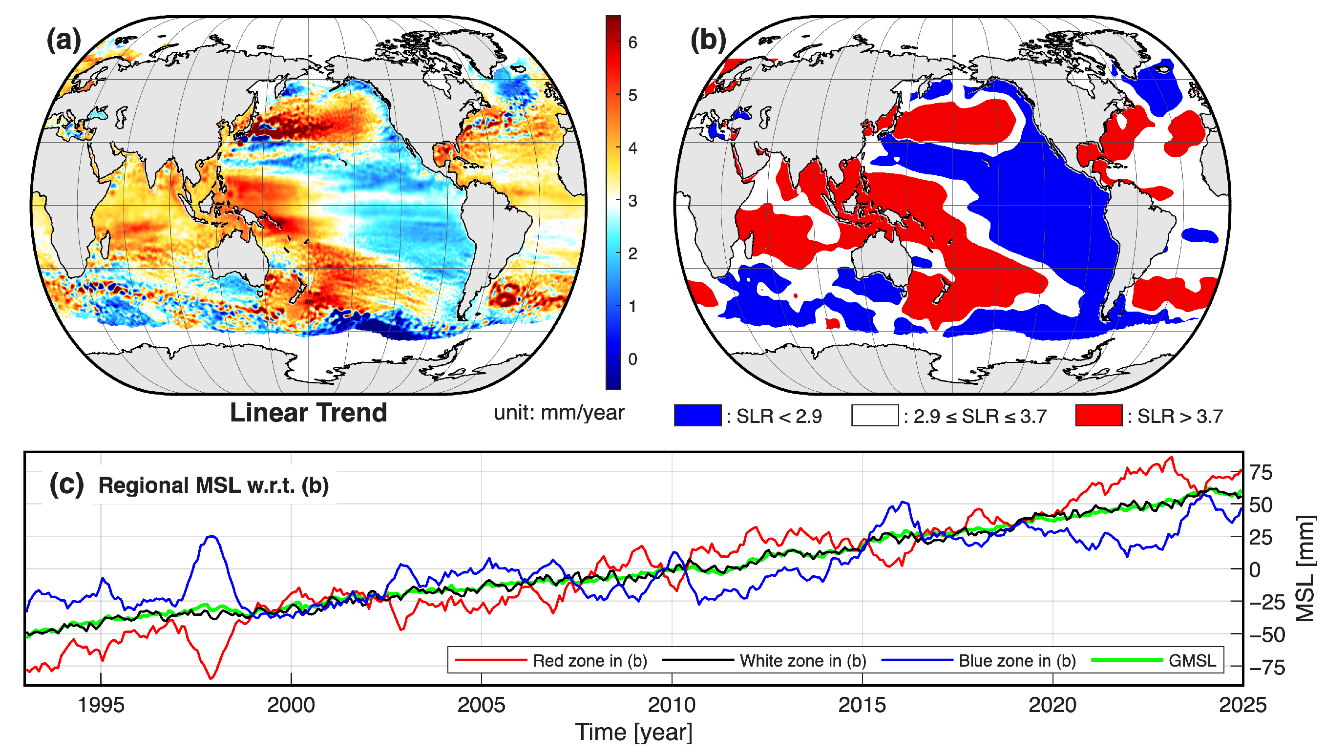
Treatment of sea-level trend uncertainties. Several quantities with units of mm yr⁻¹ are reported in this study, but they do not all represent the same type of estimate. Published global mean sea-level rates are quoted with their reported uncertainties where available. In contrast, the gridded regional trends shown in Figure 1a and the tercile thresholds used for the regional classification in Figure 1b are deterministic least-squares estimates derived from the processed DUACS regional trend field. These values are used to describe the spatial pattern of satellite-era regional sea-level change and to define diagnostic regional categories.

The primary uncertainty quantified in this study is the model-based empirical contribution of internally generated climate variability to regional sea-level trend estimates. This component is estimated using the unforced CESM random-window analysis described in Section 3.4 and is expressed as the location-specific quantity $U_{99}(r,T)$. Thus, the empirical intervals reported in Figure 2 quantify the internally generated component of trend uncertainty associated with the leading EOF mode. They do not include DUACS mapping errors, inter-mission calibration uncertainty, geophysical correction uncertainty, GIA-related bias, regression uncertainty associated with temporally autocorrelated residuals, or uncertainty in the forced sea-level response.

Correlation coefficients and empirical intervals. Pearson correlation coefficients are reported as descriptive measures of linear association between the EOF principal component time series, regional mean sea-level time series, and climate indices. Because these monthly time series are serially autocorrelated, no standard independent-sample confidence intervals are reported for the Pearson correlations. The model-based 99% empirical intervals discussed in Section 3.4 and Figure 2 refer to the empirical distribution of CESM-derived trend coefficients, not to confidence intervals for Pearson correlation coefficients.

2.5. IPO Index Definitions

Three distinct IPO-related indices are used in this study, each serving a different purpose, and are summarized here to avoid ambiguity.

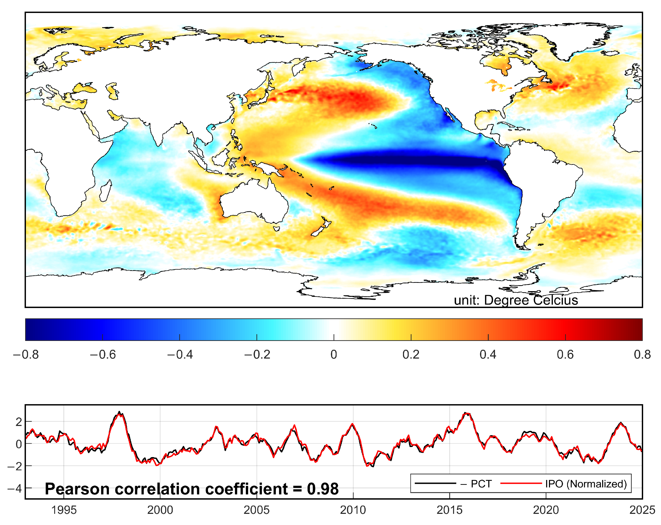
The first is an observational IPO index derived from the NOAA OISST dataset, defined as the PCT of the leading EOF mode of deseasonalized and detrended global SST anomalies over January 1993–December 2024 (Figure A3). This index follows the broad approach of Henley et al. [31] and is used as the primary observational benchmark for comparison with satellite-derived sea-level variability in Section 3.1 and Section 3.2. The second is the Henley et al. [31] tripole index, which is based on area-averaged SST differences across three fixed Pacific regions. This externally published index is used solely for the supplementary correlation comparison in Figure A2, providing an independent cross-check against the OISST-based index. The third is a model-derived IPO index, computed separately for each of the 100 unforced CESM segments as the PCT of the leading EOF mode of the corresponding CESM SST field, following the same deseasonalization and detrending procedure as applied to the observational data. This index is used exclusively for internal validation within the CESM ensemble in Section 3.3.

3. Results

3.1. Regional Sea-Level Trend Pattern from Satellite Altimetry

The linear trend map of satellite-altimeter-derived sea-level anomalies for January 1993–December 2024 reveals substantial regional heterogeneity in sea-level rise (Figure 1a). This analysis is based on the gridded DUACS regional sea-level anomaly product, processed over the study-specific ocean mask and latitude range, and is intended to examine spatially heterogeneous regional trend patterns rather than to provide an independent estimate of the reference global mean sea-level rise rate. For this reason, the area-weighted properties of the gridded DUACS trend field should not be directly compared with the reference-mission global mean sea-level estimate reported by Hamlington et al. [2]. Instead, the following analysis focuses on the relative spatial distribution of regional sea-level trends within the processed DUACS field.

The gridded trend values in Figure 1a are presented as pointwise least-squares estimates of the regional trend pattern. Full observational uncertainties are not assigned to each grid cell in this map because the present analysis does not propagate the DUACS product-error covariance, inter-mission calibration uncertainty, geophysical correction uncertainty, or GIA-related uncertainty through the trend and EOF analyses. Instead, the uncertainty analysis in Section 3.4 quantifies the model-based internal-variability component of regional trend uncertainty, which is the focus of this study.

Regions of markedly elevated SLR are concentrated in the western tropical Pacific and parts of the Indian Ocean, while regions of comparatively low or near-zero SLR are observed across much of the eastern Pacific and portions of the high-latitude Southern Ocean. These broad features are consistent with the regional trend structure documented in earlier segments of the satellite record [4,22], confirming the persistence of a strong east–west Pacific asymmetry throughout the full 32-year period. The range of regional trends extends from well below zero to substantially above the reference global mean rate reported in independent GMSL products in some locations, underscoring the degree to which local sea-level change can deviate from the global average during the satellite era.

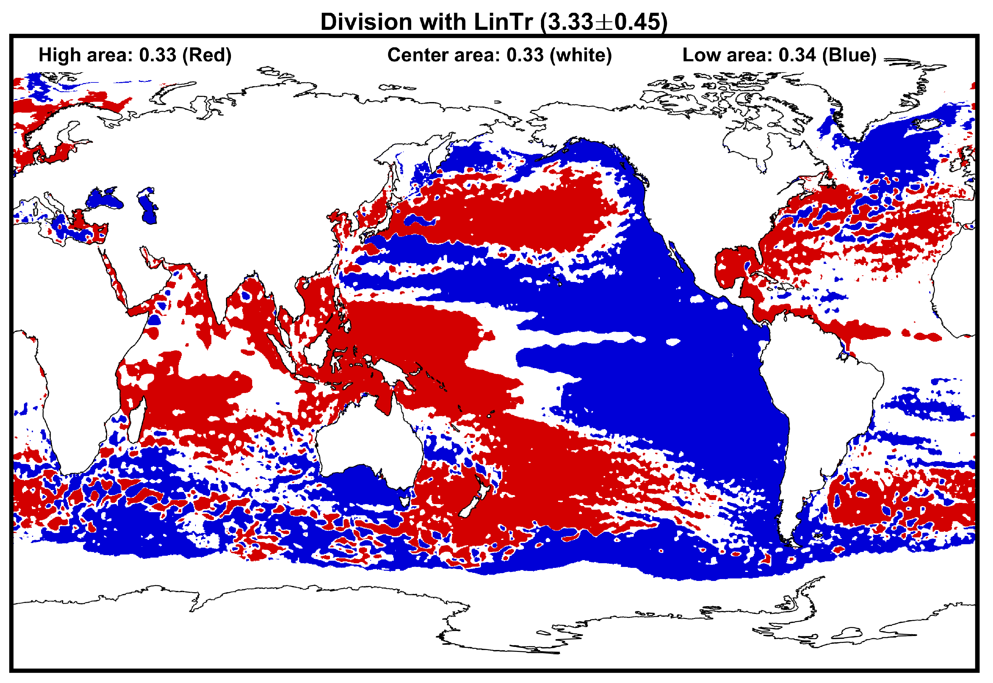
To classify the spatial structure of the satellite-derived regional trend pattern, the gridded trend field was divided into three area-weighted categories. The threshold values of $2.9$ and $3.7\mathrm{mm}{\mathrm{yr}}^{-1}$ were selected as the lower and upper area-weighted tercile thresholds of the regional trend distribution over the valid ocean grid points. The resulting low-, intermediate-, and high-trend regions occupy 33.0%, 34.0%, and 33.0% of the valid ocean area, respectively. Thus, these thresholds are used to define approximately equal-area diagnostic categories for comparing regions of relatively low and high satellite-era sea-level trends, rather than as physically fixed sea-level-rise thresholds, estimates of the global mean sea-level trend, or uncertainty-bounded local trend estimates.

To facilitate quantitative comparison between high- and low-trend regions, the global ocean was partitioned into three zones based on the spatially smoothed Gaussian-filtered trend field (Figure 1b): high-trend regions (SLR $>3.7\mathrm{mm}{\mathrm{yr}}^{-1}$), intermediate-trend regions ($2.9\le$ SLR $\le 3.7\mathrm{mm}{\mathrm{yr}}^{-1}$), and low-trend regions (SLR $<2.9\mathrm{mm}{\mathrm{yr}}^{-1}$). The threshold values of $2.9$ and $3.7\mathrm{mm}{\mathrm{yr}}^{-1}$ were selected such that the three zones subtend approximately equal ocean surface areas when integrated over the analysis domain, thereby ensuring that the regional mean sea-level time series in each zone are computed from comparable spatial samples and are not disproportionately weighted toward any single basin. The zonal boundaries were defined after applying a Gaussian filter with a five-standard-deviation span to remove small-scale features; the unsmoothed trend map and zone boundaries are shown for reference in Figure A1.

Regional mean sea-level time series computed for the high- and low-trend zones exhibit strong anti-correlation ($r=-0.98$) and are approximately symmetric about the global MSL time series (Figure 1c). This strong anti-correlation is a hallmark of a spatially coherent, basin-scale redistribution of sea level, rather than a pattern driven by locally independent processes. The large-amplitude interannual and decadal variability present in both regional MSL time series, superimposed on the rising global mean, indicates that the zonal boundaries are not stationary: the partitioning of the ocean into high- and low-trend regions would shift substantially if computed over a different time interval. This behavior is consistent with prior studies demonstrating that the satellite-era regional SLR pattern is sensitive to the choice of analysis period [10,11,23,26].

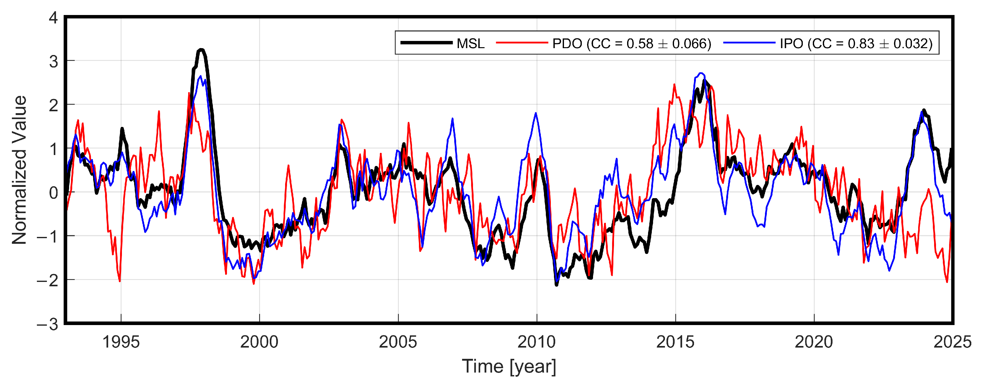
To investigate the connection to large-scale climate variability, the detrended and normalized low-zone regional MSL (blue line, Figure 1c) is compared to the Pacific Decadal Oscillation (PDO) index and the Interdecadal Pacific Oscillation (IPO) index [31,32]. Both indices are significantly correlated with the regional MSL (PDO: $r=0.68$; IPO: $r=0.81$; similar correlations, but with opposite sign, hold for the high-trend zone), as shown in Figure A2. The higher correlation with the IPO, which is defined as the leading EOF mode of global SST and thus reflects a broader spatial pattern of coupled ocean–atmosphere variability than the North Pacific-focused PDO, motivates its use as the primary climate index for subsequent EOF-based analysis.

3.2. Leading EOF Mode of Satellite-Observed Sea Level

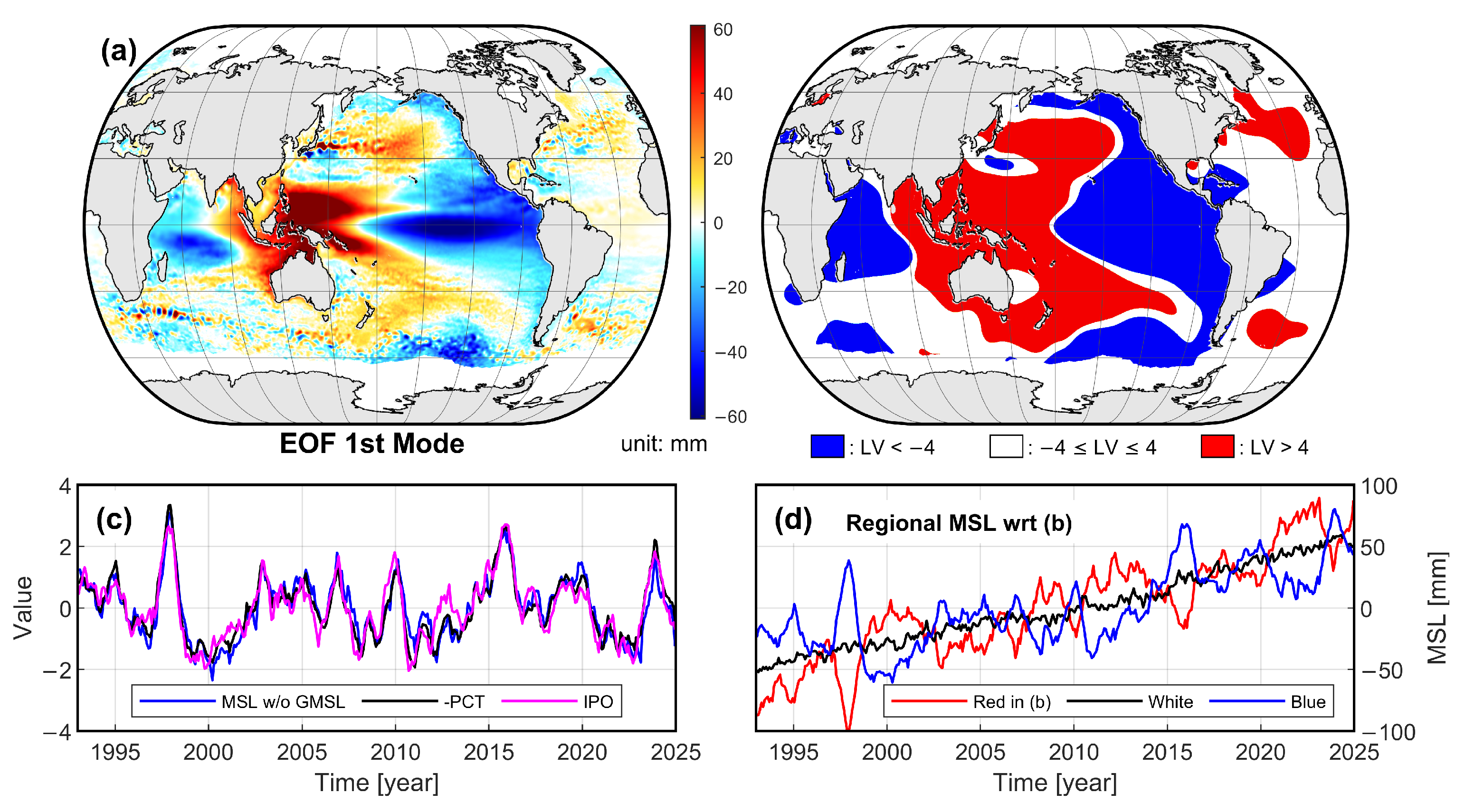
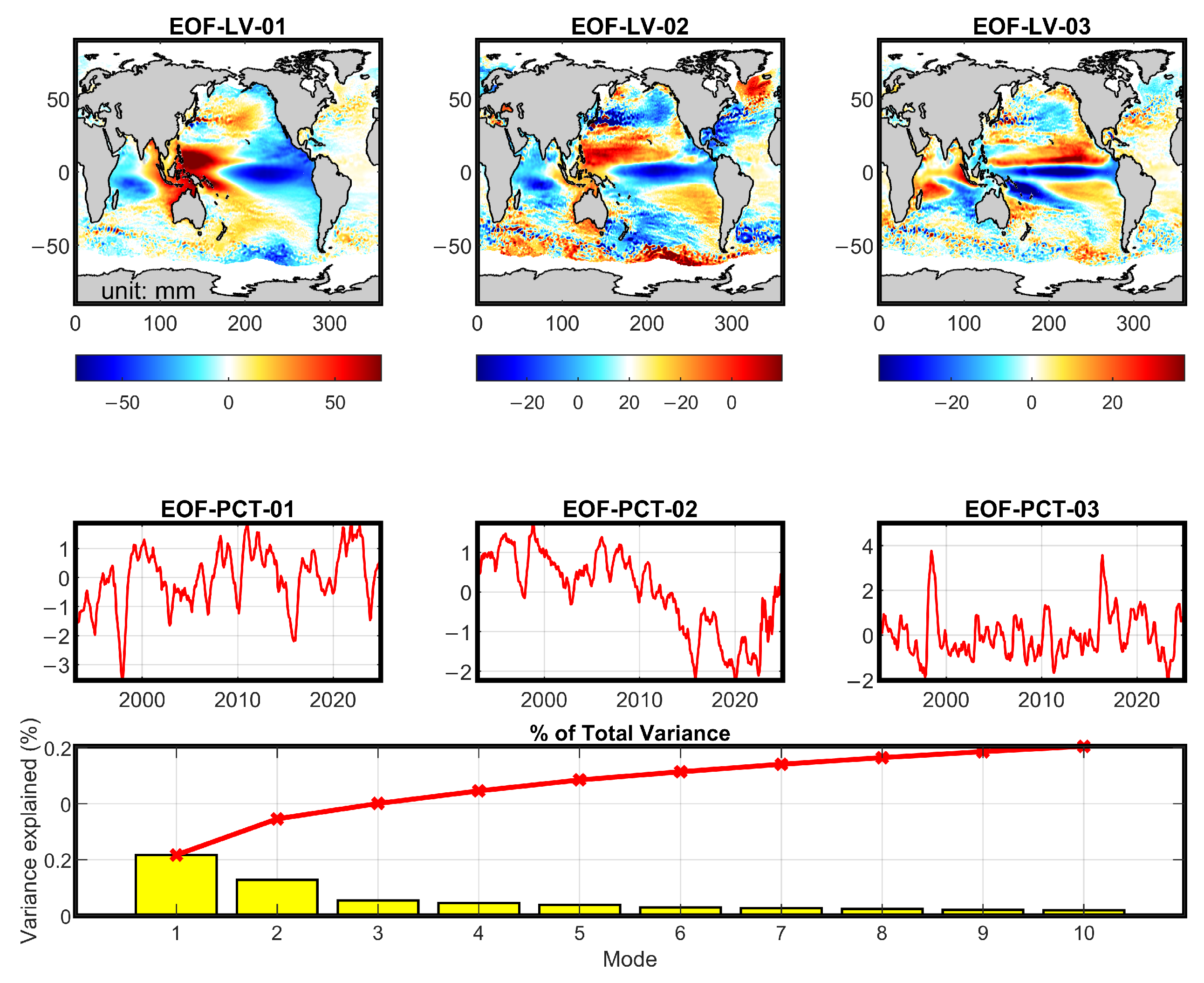
To move beyond a trend-map perspective and identify the leading spatial mode of regional sea-level variability, EOF analysis was applied to the deseasonalized, detrended, and cosine-latitude-weighted monthly SLA anomaly fields over January 1993–December 2024. The first three EOF modes explain 10.9%, 6.45%, and 2.75% of the total monthly SLA variance, respectively. The separation between the first and second modes satisfies the North et al. [28] criterion, indicating that the leading mode is statistically distinct from the second mode and is not strongly affected by mode mixing. However, because the leading mode explains only 10.9% of the total variance, it should not be interpreted as representing the majority of all regional sea-level variability. Its relevance to the 1993–2024 trend pattern arises instead from its low-frequency evolution, its close relationship with the IPO index, and its spatial projection onto the observed large-scale east–west contrast in regional sea-level trends.

The first loading vector (LV₁; Figure 3a) exhibits a large-scale dipolar structure: positive anomalies dominate the western tropical Pacific and parts of the Indian Ocean, while negative anomalies prevail across the eastern tropical and subtropical Pacific. This spatial pattern closely resembles the known sea-surface-height signature of IPO/PDO variability [17,21,27] and is consistent with the wind-driven redistribution of upper-ocean heat and mass associated with decadal modulation of the Pacific trade winds. At the same time, the modest variance explained by EOF1 indicates that this IPO-like mode provides only a partial description of satellite-era regional sea-level variability. Noticeable departures from the leading Pacific-centered pattern are observed in the western Indian Ocean and the North Atlantic, where the leading EOF explains less of the local variability. These departures suggest that additional modes and basin-specific processes, including Indian Ocean Dipole-related variability, Atlantic multidecadal variability, regional wind forcing, steric changes, and ocean circulation variability, are also important for characterizing regional sea-level variability in those basins [33,34].

The PCT of the first EOF mode (PCT₁; Figure 3c) is highly correlated with the IPO index ($r=0.92$) and with the detrended regional MSL of the low-LV zone after removing global MSL (r = 0.86). These high correlations indicate that PCT₁ is not merely a statistical artifact of the EOF decomposition but captures a physically meaningful mode of variability linked to basin-scale decadal climate variability. To construct EOF-based regional zones analogous to those in Section 3.1, a threshold of $\pm 4$ mm was applied to the spatially smoothed LV₁ field (Figure 3b). The resulting high- and low-variability zones broadly resemble the trend-based zones of Figure 1b, particularly in the tropical Pacific. The most notable differences occur in the western Indian Ocean and North Atlantic, again indicating that the leading EOF mode captures a prominent IPO-like component of the observed regional trend structure, but does not fully explain regional trend heterogeneity in all basins.

The regional MSL time series computed from these EOF-based zones (Figure 3d) are strongly correlated with both PCT₁ $(r=0.97)$ and the IPO index $(r=0.92)$. Taken together, these results indicate that the leading mode of satellite-altimeter-derived regional sea-level variability during 1993–2024 is closely linked to decadal-scale IPO-like climate variability. This finding is consistent with, as well as extending to the updated 32-year record, earlier analyses covering shorter altimeter periods [14,18,20]. Nevertheless, because EOF1 explains a limited fraction of the total monthly SLA variance, the IPO-like mode should be interpreted as an important but incomplete component of satellite-era regional sea-level variability, with secondary modes and basin-specific processes remaining important, especially outside the tropical Pacific.

3.3. Representation of Internal Variability in Unforced CESM

The results of Section 3.2 establish that the leading EOF mode of the satellite sea-level record is closely linked to IPO-like internal variability. However, the satellite altimeter record constitutes only a single 32-year realization of the climate system, which includes both internally generated variability and the forced response to historical radiative forcing. To assess whether the leading statistical mode identified from the satellite data is consistent with internally generated variability, the same EOF analysis was applied to the 100-member ensemble of unforced CESM 100-year sea-level segments described in Section 2.3.

A necessary premise of this comparison is that the externally forced sea-level response and the unforced internal mode are associated with distinguishable spatial patterns; if the forced response projected onto the same IPO-like dipole, similarity to the unforced CESM mode would carry little diagnostic value. This premise is supported by previous studies that separated forced and internal components using large ensembles and observational analyses. Using ensemble averaging of CESM and CMIP5 large-ensemble historical simulations, Fasullo and Nerem [6] showed that the forced sea-level pattern is spatially broad and smooth—characterized by an enhanced rise in the Southern Ocean, the subpolar North Atlantic, and low latitudes—and is structurally distinct from the sharply dipolar Pacific pattern associated with internal decadal variability. Consistently, Hamlington et al. [27] isolated the forced pattern in the satellite record after removing internal decadal (PDO-related) variability and obtained a spatially smooth, basin-coherent rise rather than an east–west Pacific dipole. The forced and internally generated patterns are therefore distinguishable at large scales, which preserves the diagnostic value of the unforced comparison performed here. An important exception is the tropical Pacific, where forced wind-driven circulation changes can project onto a pattern locally resembling the internal dipole [11]; for this reason, the comparison below is framed as a consistency assessment rather than a formal attribution test.

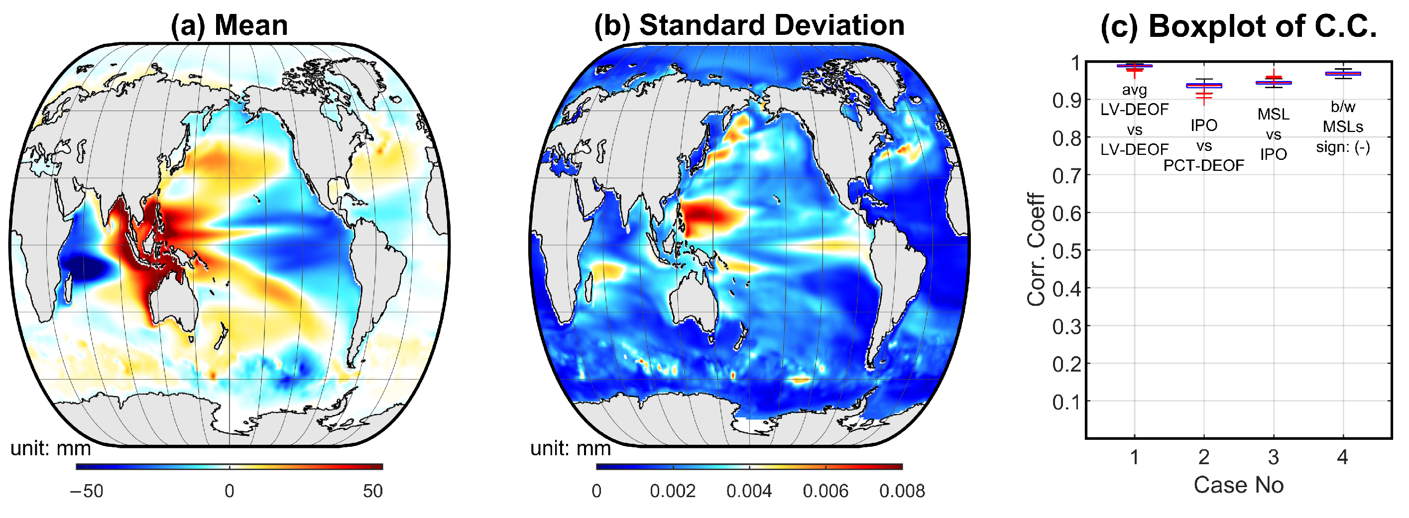
Figure 4a shows the ensemble mean of the 100 dominant EOF modes (hereafter DEOF) computed from the unforced CESM, and Figure 4b shows the corresponding ensemble standard deviation, which provides a measure of the across-realization spread in the dominant natural variability pattern. The ensemble mean DEOF exhibits a large-scale spatial structure closely resembling that of LV₁ from the satellite analysis (Figure 3a): positive anomalies concentrated in the western tropical Pacific and negative anomalies in the eastern Pacific. The cross-member spatial correlation between the ensemble mean DEOF and each individual DEOF is very high (mean r = 0.99; Figure 4c, column 1), indicating that this IPO-like structure is a robust feature of internally generated variability in the model ensemble, rather than a pattern dependent on a single 100-year sample.

The correlations between each DEOF’s PCT and the corresponding model-derived IPO index (defined as the PCT of the leading SST EOF from the same simulation segment; Section 2.5) are similarly high (mean r = 0.94; Figure 4c, column 2), supporting the interpretation that the dominant mode of unforced sea-level variability in CESM is associated with an IPO-like SST pattern comparable to that linked to the satellite-observed sea-level variability.

Further, the regional MSL time series computed from CESM-derived zones are strongly correlated with the corresponding DEOF PCTs (Figure 4c, columns 3–4), paralleling the observational analysis in Section 3.2. The close quantitative agreement between the spatial patterns and temporal correlations of the satellite-derived dominant mode (Figure 3) and the unforced CESM dominant mode (Figure 4) supports two key conclusions. First, the dominant EOF mode of satellite-altimeter-derived sea-level variability is consistent with internally generated IPO-like decadal variability, because a similar mode emerges in the absence of external radiative forcing in the unforced CESM simulation. Second, the unforced CESM consistently exhibits a spatially similar mode across 100 100-year samples, supporting its use as a statistical baseline for estimating the internal-variability contribution to regional trend uncertainty. These findings are broadly consistent with the wider literature showing that internal Pacific decadal variability dominates the regional sea-level trend pattern during the satellite era [6,14,15,23].

3.4. Record-Length Dependence of Natural-Variability-Induced Trends

Having shown that the leading mode of satellite-observed sea-level variability is consistent with IPO-like variability represented in the unforced CESM, we now quantify how the contribution of this mode to estimated regional sea-level trends changes with the length of the observational record. This analysis is motivated by the recognition that, as the satellite altimeter record continues to lengthen, the influence of decadal internal variability on trend estimates should diminish as an increasing number of complete IPO cycles are sampled [6,10,13].

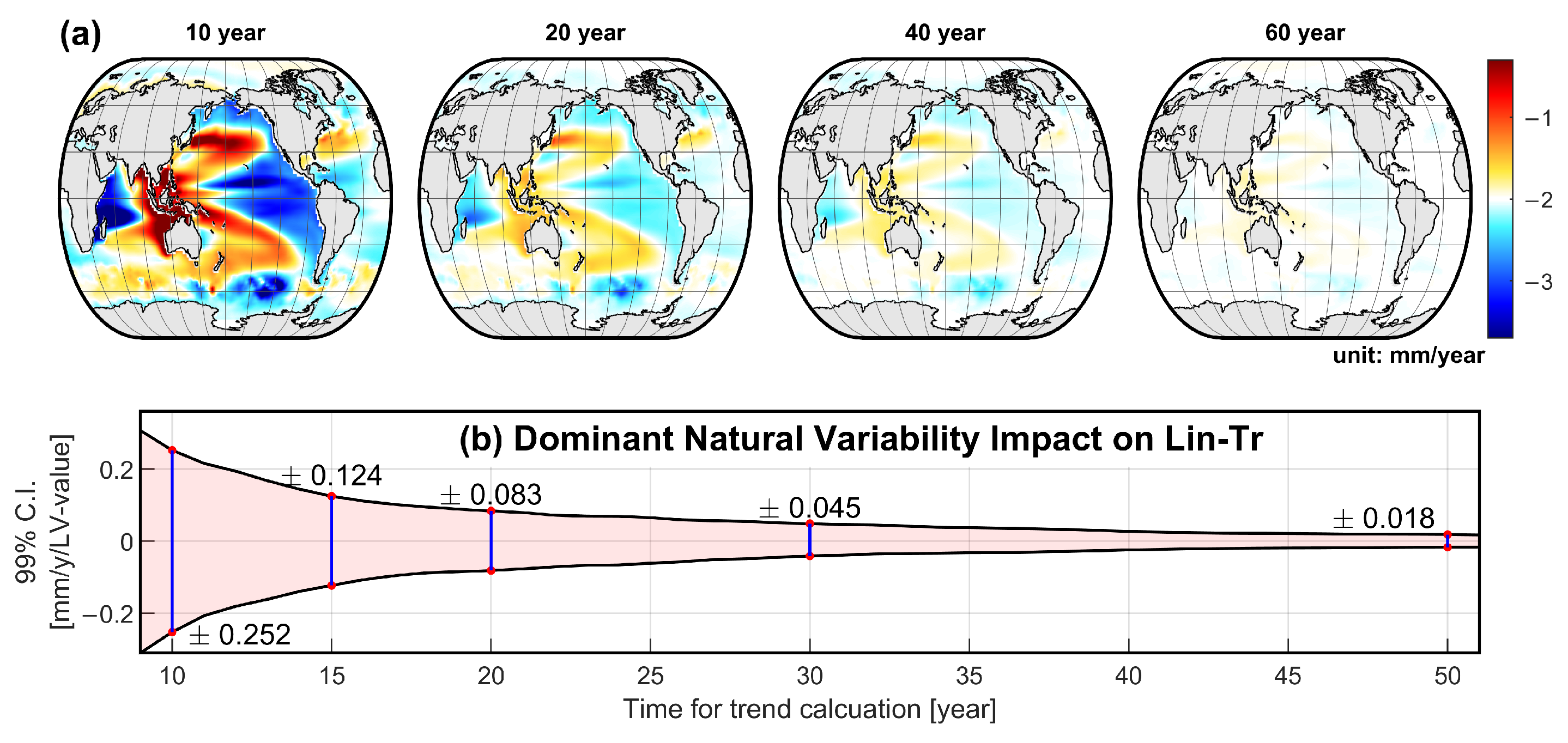
Linear sea-level trend patterns were computed over four target record lengths of 10, 20, 40, and 60 years using the random-window sampling procedure applied to each of the 100 unforced CESM segments, as described in Section 2.3. EOF analysis was then applied to each ensemble of trend patterns following Meyssignac et al. [18] and Hamlington et al. [20]. Figure 2a shows the ensemble-mean dominant EOF of the trend patterns, hereafter referred to as the dominant natural trend mode (DNTM), for each record length. The spatial structures of the DNTMs across all four record lengths closely resemble both the DEOF from the variability analysis (Figure 4a) and the leading LV₁ from satellite observations (Figure 3a), suggesting that an IPO-like spatial pattern represents a persistent component of internally generated trend variability across the record lengths considered.

Each DNTM accounts for approximately 20% of the total trend variance, a fraction that is largely insensitive to record length, indicating that IPO-like internal variability represents a persistent and structurally stable source of trend uncertainty across all record lengths examined here.

To apply the EOF-based uncertainty scaling, we use the normalization convention and notation defined in Section 2.4. In particular, Equation (2) defines the trend coefficient ${\beta }_T$ of the normalized dominant-mode PCT for a given record length T, and Equation (3) converts this dimensionless PCT trend into a local sea-level trend contribution with units of mm yr⁻¹. The model-based 99% empirical half-width, $h_{99}\left(T\right)$, is defined from the empirical distribution of ${\beta }_T$ in Equation (4), and the corresponding location-specific internal-variability-induced empirical trend uncertainty, $U_{99}(r,T)$, is defined in Equation (5).

For each record length T, the empirical distribution of ${\beta }_T$ was obtained from the 10,000 random-window CESM samples. This distribution was then used to compute $h_{99}\left(T\right)$ and, by applying Equation (5), to estimate the internally generated component of regional sea-level trend uncertainty at each grid point. This quantity represents only the model-based empirical spread associated with the leading internal-variability mode and should not be interpreted as a complete observational uncertainty estimate.

Critically, however, while the spatial structure of the dominant natural trend mode is stable, its amplitude decreases systematically as the record length increases (Figure 2a). The amplitude reduction reflects the tendency for longer trend estimates to average over more complete cycles of decadal variability, thereby reducing the influence of the particular phase of the IPO captured during the observational window. This result is consistent with theoretical expectations and previous modeling studies [18,20,22]: longer records are less susceptible to aliasing by decadal internal variability.

The model-based 99% empirical intervals shown in Figure 2b were constructed from 10,000 random-window estimates of ${\beta }_T$ for each record length. Specifically, for each target record length and each 100-year CESM segment, 100 starting months were randomly selected without replacement from all possible starting months, and the corresponding linear trends of the normalized dominant-mode PCT were computed over the selected windows. This procedure was repeated for all 100 CESM segments. Because some overlap among randomly selected windows may still occur, especially for longer record lengths, these intervals should be interpreted as model-based empirical intervals of internally generated trend variability rather than as formal confidence intervals based on statistically independent realizations.

The empirical intervals decrease monotonically and approximately inversely with record length, consistent with the expected decrease in trend uncertainty as longer records average over more phases of decadal variability. For a representative grid point with an LV₁ amplitude of 40 mm, the model-based 99% empirical interval of the dominant internal-variability contribution to the regional SLR trend is approximately $\pm 3.31$ mm yr⁻¹ for a 20-year record and $\pm 1.80$ mm yr⁻¹ for a 30-year record. At the current satellite record length of 32 years, this empirical interval reduces to approximately $\pm 1.61$ mm yr⁻¹ (corresponding to $h_{99}\approx$ 0.040 yr⁻¹ for the normalized dominant-mode PCT; cf. Figure 2b), which remains comparable in magnitude to typical regional deviations from the global mean trend.

These values quantify only the internally generated component associated with the leading EOF mode and should not be interpreted as complete observational uncertainties for the corresponding satellite-derived regional trend estimates. At 60 years, the corresponding model-based internal-variability uncertainty becomes substantially smaller, which would facilitate improved detection of the forced regional sea-level signal, depending on the amplitude and spatial structure of the forced response, consistent with the time-of-emergence estimates of Lyu et al. [13].

Taken together, the results of Section 3.1, Section 3.2, Section 3.3 and Section 3.4 establish a coherent and internally consistent picture: the dominant spatial pattern of regional sea-level trends observed during the satellite-altimetry era is substantially influenced by IPO-like internal climate variability; a similar IPO-like variability mode is consistently represented in the unforced model simulations; and its contribution to estimated regional trends, while persistent in structure, decreases approximately inversely with record length. These findings imply that the forced regional sea-level signal will become progressively more detectable as the satellite altimeter record continues to grow beyond its current 32-year extent, while the present record remains substantially influenced by internal climate variability.

4. Discussion

4.1. Implications for the Interpretation of Satellite-Altimeter-Derived Trend Maps

A primary motivation for this study is that regional sea-level trend maps derived from satellite altimetry are widely used as indicators of long-term sea-level change in the remote sensing community, including in climate assessments, model validation studies, and coastal planning applications [12,35]. Our results caution against interpreting such maps as direct representations of the forced regional sea-level response alone. The leading EOF mode of the 32-year DUACS altimetry record is strongly related to IPO-like variability, as indicated by the high correlation between its PCT and the IPO index ($r=0.92$) and by the emergence of a spatially similar mode across the unforced CESM samples. However, this leading mode explains only 10.9% of the total monthly SLA variance and therefore should not be interpreted as explaining the majority of all regional sea-level variability.

The relevance of the leading IPO-like mode to the satellite-era trend pattern arises from its low-frequency evolution and its strong spatial projection onto the large-scale east–west contrast in regional sea-level trends during 1993–2024. Thus, a prominent component of the spatial heterogeneity visible in current satellite-altimeter trend maps may reflect the particular phase of decadal-to-multidecadal internal variability sampled during the satellite era, in addition to any spatially structured forced sea-level response. Because this study does not perform a formal forced–unforced detection-and-attribution analysis, these contributions cannot be fully separated here. Practitioners using satellite-altimeter trend maps should therefore interpret regional trend estimates with caution, particularly in regions where the local EOF amplitude is large (Figure 3a).

The EOF-based scaling framework developed in Section 3.4 provides a practical way to estimate the internally generated component of regional sea-level trend uncertainty. Specifically, the model-based empirical interval derived from the unforced CESM simulation can be scaled by the local loading amplitude of the leading internal-variability mode to obtain a location-specific estimate of the internal-variability contribution to trend uncertainty. This estimate should not be interpreted as a complete uncertainty bound for DUACS-derived regional trends, because it does not include DUACS mapping errors, inter-mission calibration uncertainty, geophysical correction uncertainty, GIA-related bias, or uncertainty in the forced sea-level response.

The relatively modest variance explained by EOF1 also highlights the importance of secondary modes and basin-specific processes. While the leading IPO-like mode provides a useful framework for interpreting the prominent Pacific-centered east–west contrast during the satellite era, it cannot fully explain regional trend heterogeneity in all basins. The secondary EOF modes should therefore not be interpreted simply as residual noise. Rather, they likely represent additional components of regional sea-level variability that can become important outside the tropical Pacific and provide the basis for interpreting basin-specific departures from the leading Pacific-centered pattern.

Although the leading IPO-like mode provides the clearest large-scale structure in the present analysis, the regional sea-level trend field should not be interpreted as a Pacific-only phenomenon. In the Indian Ocean, regional sea-level variability may reflect a combination of remote Pacific influence and basin-specific processes, including Indo-Pacific wind forcing, basin-scale thermosteric changes, Indian Ocean Dipole-related variability, monsoon-related circulation changes, and oceanic adjustment to Pacific decadal variability [11,21,34]. In the Atlantic Ocean, regional sea-level changes may involve gyre circulation, wind stress, buoyancy forcing, freshwater input, and changes in large-scale overturning circulation, and thus cannot be interpreted solely through the Pacific-centered IPO-like mode [12,33]. In the Southern Ocean, sea-level trends are influenced by strong zonal winds, steric changes, eddy compensation, and the reduced reliability of satellite altimetry near sea-ice-affected regions, which motivates the latitude limit applied in this study. These basin-to-basin differences reinforce the interpretation that the EOF-based uncertainty framework developed here is best viewed as a diagnostic estimate of the internal-variability contribution associated with the leading mode, rather than as a complete basin-by-basin attribution of regional sea-level change. A full explanation of regional differences across all ocean basins would require targeted analyses of secondary EOF modes, basin-specific climate indices, ocean circulation diagnostics, and multi-model forced and unforced simulations.

4.2. Relationship to Recent Studies

The findings of this study are broadly consistent with, and extend, a growing body of recent literature on the drivers of satellite-era regional sea-level trends. Before interpreting the similarity between the satellite-era EOF and the unforced CESM modes, it is important to distinguish the externally forced response from internally generated variability. In forced large-ensemble analyses, the externally forced component is represented by the ensemble-mean response, whereas IPO-like fluctuations in individual forced members arise from internal variability superimposed on the forced signal and are largely removed by ensemble averaging so that the ensemble-mean response isolates the forced pattern. Thus, the unforced CESM IPO-like mode analyzed here should be interpreted as a distinct internally generated component, rather than as a pattern that is necessarily common to all forced and unforced model variations.

Karnauskas et al. [11] investigated regional sea-level change over the altimeter era using satellite observations, forced large ensembles, and single-forcing experiments. Their analysis showed that externally forced wind-driven circulation changes, including Ekman and Sverdrup dynamics, can explain important features of the observed regional trend pattern. This forced ensemble-mean response is dynamically distinct from the IPO-like mode extracted from the unforced CESM control simulation in the present study, which arises in the absence of external radiative forcing. Therefore, the similarity between the satellite-era pattern and the unforced CESM mode is interpreted here as evidence that internally generated variability can strongly project onto the observed regional trend pattern, not as evidence that the observed pattern is purely unforced. The forced and internal contributions can nonetheless project onto similar patterns in the tropical Pacific, where wind-driven circulation changes and IPO-like variability are dynamically related. The two frameworks therefore address complementary aspects of the same regional trend pattern: attribution of the forced contribution versus empirical bounding of the internal-variability component. The possibility of partial overlap in the tropical Pacific does not undermine the large-scale distinction between the forced and internal patterns documented by ensemble-based separations [6,27], but it identifies the region where the present consistency-based interpretation should be treated most cautiously.

Little et al. [23] applied low-frequency component analysis to Pacific tide gauge records and surface climate reconstructions, isolating three coherent modes of Pacific sea-level variability: a secular greenhouse-gas-driven rise, a nonlinear mode potentially linked to aerosol forcing with a reversal around 1980, and an IPO-linked decadal mode. The IPO-linked mode corresponds to a cyclical pattern related to a 15–30-year cycle in Pacific Ocean surface temperatures and winds. The IPO-like mode identified here is closely related to this decadal Pacific mode, providing independent support from a longer tide gauge-based analysis that IPO variability is a physically meaningful source of regional sea-level variability in the Pacific. At the same time, the existence of multiple low-frequency modes in the analysis of Little et al. [23] reinforces the point that the leading IPO-like EOF mode in the satellite record should be interpreted as one important component of regional sea-level variability, not as a complete explanation of all basin-scale trend patterns. Quantitatively, the IPO-linked decadal mode isolated by Little et al. [23] from multi-decadal tide gauge records is consistent with the leading EOF mode identified here from the 32-year satellite record. The convergence of these two independent analyses—one based on century-scale tide gauge reconstructions and the other on satellite altimetry—strengthens confidence that the IPO-like signal identified in the present study reflects genuine low-frequency internal variability rather than a satellite-era artifact.

Hamlington et al. [2] demonstrated that the rate of global mean sea-level rise has nearly doubled over the satellite era, increasing from approximately $2.1\mathrm{mm}{\mathrm{yr}}^{-1}$ in 1993 to approximately $4.5\mathrm{mm}{\mathrm{yr}}^{-1}$ by 2023. This documented acceleration of the global mean rate strengthens the case that a forced sea-level signal is increasingly present in the satellite record. However, our results suggest that even as the global mean forced signal strengthens, the regional spatial pattern of the forced response may remain difficult to isolate over the current satellite period. The leading IPO-like internal mode continues to impose a substantial spatial structure on the regional trend pattern, and the model-based internal-variability contribution to trend uncertainty can remain comparable to regional deviations from the global mean for record lengths of 20–30 years. The acceleration documented by Hamlington et al. [2] thus reinforces, rather than undermines, the need for record-length-dependent estimates of the internal-variability component of regional trend uncertainty.

4.3. Limitations

Several limitations of the present analysis should be acknowledged.

Single climate model. This study relies exclusively on the CESM pre-industrial control simulation to characterize the statistics of unforced internal variability. While CESM is a well-validated and widely used coupled climate model [9], the amplitude, periodicity, spatial structure, and sea-level teleconnections of IPO-like variability differ across CMIP-class models [13]. Therefore, the model-based empirical intervals shown in Figure 2b should be interpreted as conditional on CESM’s representation of Pacific decadal variability. If CESM overestimates the amplitude of IPO-related sea-level variability or its teleconnection to regional sea level, the empirical intervals and the resulting values of $U_{99}(r,T)$ may be too large. Conversely, if CESM underestimates IPO variability, the internal-variability-induced trend uncertainty may be underestimated. Differences in IPO periodicity across models could also affect the apparent record-length scaling, because the averaging of internal variability depends on how many variability cycles are sampled within a given record length. Thus, the spatial pattern identified here is best interpreted as a CESM-based estimate of the dominant internally generated trend uncertainty, rather than as a model-independent uncertainty bound. Future work using multi-model pre-industrial control simulations, such as CMIP6 models, would be needed to test the robustness of both the spatial pattern and the quantitative record-length scaling derived here.

No direct forced/unforced separation. The analysis does not directly compare unforced and historically forced CESM simulations, which would allow an explicit attribution of the observed satellite trend pattern to forced versus internally generated components. Instead, the large-scale distinction between the forced and unforced patterns is supported by previous large-ensemble separations [6,27], which indicate that the forced pattern is relatively broad and spatially smooth compared with the internal IPO-like dipole. A direct, quantitative pattern comparison using forced CESM large-ensemble output—together with member-level detection-and-attribution analysis—remains an important direction for future work, particularly for the tropical Pacific where the two components may partially overlap [11].

GIA correction. No glacial isostatic adjustment (GIA) correction is applied to the DUACS altimetry product used in this study. Over most of the open ocean, GIA-induced geocentric sea-level changes are small, typically $0.1$–$0.5\mathrm{mm}{\mathrm{yr}}^{-1}$ [25], and spatially smooth compared to the large-amplitude IPO-like trend patterns analyzed here. GIA therefore has a negligible effect on the EOF decomposition and regional zone classification, but may introduce a small spatially varying bias in the absolute trend magnitudes reported in Figure 1a.

EOF mode mixing. EOF analysis decomposes variance into orthogonal modes that do not necessarily correspond one-to-one to distinct physical processes. In particular, the potential for mode mixing, in which a single physical signal is distributed across multiple EOF modes or multiple signals project onto a single mode, cannot be excluded, especially in regions such as the western Indian Ocean and North Atlantic where the first EOF explains less local variance (Section 3.2). The North et al. [28] rule indicates that the first mode is well-separated from the second over the 32-year satellite record, but this separation cannot be guaranteed to hold uniformly across all 100 CESM segments and all record lengths.

Segment and random-window dependence. The 100 CESM segments were sampled from a single continuous pre-industrial control integration and therefore cannot be regarded as fully independent realizations. Although the segment starting years were selected to maximize temporal separation where possible, some dependence among samples may remain, particularly for variability on centennial or longer timescales. In addition, the random-window trend estimates used in the record-length analysis are not fully independent, because windows sampled from the same 100-year segment may partially overlap, especially for longer record lengths. For this reason, the intervals shown in Figure 2b are interpreted as model-based empirical intervals describing the spread of internally generated trend estimates, rather than as formal confidence intervals derived from statistically independent realizations. This limitation is unlikely to materially affect the IPO-like spatial pattern emphasized here, whose dominant timescale is approximately decadal to multidecadal, but it should be considered when interpreting the ensemble spread and the quantitative empirical uncertainty estimates.

Observational product uncertainty. The DUACS gridded altimetry product carries observational and processing uncertainties arising from the Optimal Interpolation procedure, the density of the along-track ground-track network, inter-mission calibration, geophysical corrections, and mapping errors [24]. These uncertainties are not propagated through the EOF analysis in this study and are not included in the model-based empirical intervals shown in Figure 2b. The intervals reported here quantify only the internal-variability contribution inferred from the unforced CESM simulation. Therefore, the gridded rates shown in Figure 1a and the regional thresholds used in Figure 1b should be interpreted as trend estimates and diagnostic classification values, respectively, not as trend estimates with complete observational uncertainty bounds. A full uncertainty budget for satellite-altimeter-derived regional sea-level trends would require combining observational product uncertainty, regression uncertainty under temporally correlated residuals, GIA-related uncertainty, forced-response uncertainty, and multi-model estimates of internally generated variability.

4.4. Practical Implications

Beyond its scientific contributions, this study offers a practical framework for interpreting satellite-altimeter-derived regional sea-level trend products. For any ocean grid point at which the local amplitude of the leading EOF mode is known (LV₁; Figure 3a), the model-based empirical uncertainty associated with the leading internal-variability mode can be estimated using the scaling relation defined in Equation (5). In this relation, $D_1\left(r\right)$ is the local EOF loading amplitude in mm, and $h_{99}\left(T\right)$ is the model-based 99% empirical half-width of the trend coefficient of the normalized leading-mode PCT for a record length T. Thus, $U_{99}(r,T)$ has units of mm yr⁻¹ and represents the internally generated component of regional sea-level trend uncertainty associated with the leading mode. This quantity does not include DUACS mapping errors, inter-mission calibration uncertainty, geophysical correction uncertainty, GIA-related bias, or uncertainty in the forced sea-level response.

The EOF-based scaling framework can be applied to DUACS or equivalent altimetry products as a diagnostic estimate of the internally generated component of regional trend uncertainty. This component is absent from conventional regression-based confidence intervals, which assume temporally uncorrelated or weakly autocorrelated residuals [22]. As regional sea-level trend products are increasingly used in coastal adaptation planning and in the validation of climate model projections [2,35], the ability to quantify and communicate this source of uncertainty becomes practically important. Specifically, trend estimates in the western tropical Pacific and Indian Ocean, where LV₁ amplitudes are largest, carry the greatest natural-variability-induced uncertainty and should be interpreted with particular caution until the satellite record extends to approximately 40–60 years.

5. Conclusions

This study assessed the contribution of internal climate variability to satellite-altimeter-derived regional sea-level trend patterns and quantified how this contribution changes with the length of the observational record. The analysis combined the 32-year DUACS multi-mission satellite altimetry product (January 1993–December 2024) with 100 100-year samples from an unforced CESM pre-industrial control simulation, with EOF analysis applied consistently across both datasets. The aim was not to formally separate forced and unforced contributions to the observed regional trend pattern, but to estimate the model-based contribution of internal variability to the uncertainty of satellite-altimeter-derived regional trend estimates.

Three principal findings emerge from this analysis. First, the leading EOF mode of satellite-observed regional sea-level variability, explaining 10.9% of total variance, exhibits an IPO-like dipolar spatial structure that is highly correlated with the IPO index (r = 0.92). This mode projects strongly onto the east–west asymmetry in the 32-year regional trend pattern, indicating that satellite-altimeter-derived regional sea-level trends during 1993–2024 remain substantially influenced by decadal-to-multidecadal internal climate variability, consistent with the unforced CESM analysis presented here.

Second, a similar IPO-like mode emerges consistently across the 100 unforced CESM samples, with a mean spatial correlation of 0.99 relative to the ensemble-mean CESM mode and a mean PCT–IPO correlation of 0.94. The diagnostic value of this agreement is strengthened by the previously documented distinction between the externally forced sea-level response, which is relatively broad and basin-coherent, and the sharply dipolar internal mode [6,27]; given this distinction, the agreement suggests that the leading satellite-observed pattern is strongly consistent with internally generated variability. However, because the forced and internal patterns may partially overlap in the tropical Pacific [11] and no formal forced–unforced detection-and-attribution analysis is performed, a partial forced contribution to the observed pattern cannot be excluded.

Third, based on CESM simulations, the internal-variability contribution to regional trend uncertainty decreases approximately inversely with record length (Figure 2). The IPO-like spatial structure remains stable across the different record lengths, while its amplitude and associated model-based 99% empirical interval diminish systematically. Using the EOF-based scaling framework defined in Section 2.4 and Section 3.4, this result provides a practical way to estimate the internally generated component of regional sea-level trend uncertainty at each open-ocean grid point within the analysis domain.

Taken together, these findings indicate that the current 32-year satellite altimeter record remains substantially influenced by internal climate variability in its regional trend patterns, particularly in regions where the leading internal-variability mode has large amplitudes, including the western tropical Pacific and Indian Ocean. This influence is expected to decrease as the satellite record continues to lengthen, improving the detectability of the forced regional sea-level signal. The uncertainty estimates presented here should therefore be interpreted as CESM-based empirical estimates of the internal-variability contribution to regional sea-level trend uncertainty, not as complete uncertainty bounds for satellite-altimeter-derived trends. They do not include DUACS mapping errors, inter-mission calibration uncertainty, geophysical correction uncertainty, GIA-related bias, uncertainty in the forced sea-level response, or multi-model uncertainty in internally generated variability. A complete uncertainty assessment would require combining these additional components with the internal-variability estimate developed here.

References

1. Nerem, R.S.; Beckley, B.D.; Fasullo, J.T.; Hamlington, B.D.; Masters, D.; Mitchum, G.T. Climate-change–driven accelerated sea-level rise detected in the altimeter era. Proc. Natl. Acad. Sci. USA 2018, 115, 2022–2025. [Google Scholar] [CrossRef] [PubMed]
2. Hamlington, B.D.; Bellas-Manley, A.; Willis, J.K.; Fournier, S.; Vinogradova, N.; Nerem, R.S.; Piecuch, C.G.; Thompson, P.R.; Kopp, R. The rate of global sea level rise doubled during the past three decades. Commun. Earth Environ. 2024, 5, 601. [Google Scholar] [CrossRef]
3. NASA Sea Level Change Team. Sea Level Change: Observations from Space. 2026. Available online: https://sealevel.nasa.gov (accessed on 27 May 2026).
4. Hamlington, B.D.; Gardner, A.S.; Ivins, E.; Lenaerts, J.T.M.; Reager, J.T.; Trossman, D.S.; Zaron, E.D.; Adhikari, S.; Arendt, A.; Aschwanden, A. Understanding of contemporary regional sea-level change and the implications for the future. Rev. Geophys. 2020, 58, e2019RG000672. [Google Scholar] [CrossRef] [PubMed]
5. Thompson, P.R.; Widlansky, M.J.; Leuliette, E.; Chambers, D.P.; Beckley, B.; Sweet, W.; Ablain, M.; Mitchum, G.; Merrifield, M.; Nerem, R.S. Global oceans—Sea-level variability and change [in: State of the Climate in 2023]. Bull. Am. Meteorol. Soc. 2024, 105, S183. [Google Scholar] [CrossRef]
6. Fasullo, J.T.; Nerem, R.S. Altimeter-era emergence of the patterns of forced sea-level rise in climate models and implications for the future. Proc. Natl. Acad. Sci. USA 2018, 115, 12944–12949. [Google Scholar] [CrossRef] [PubMed]
7. Slangen, A.B.A.; Church, J.A.; Zhang, X.; Monselesan, D.P. The sea level response to external forcings in historical simulations of CMIP5 climate models. J. Clim. 2015, 28, 8521–8539. [Google Scholar] [CrossRef]
8. IPCC. Annex II: Glossary. In Climate Change 2022: Impacts, Adaptation and Vulnerability. Contribution of Working Group II to the Sixth Assessment Report of the Intergovernmental Panel on Climate Change; IPCC: Geneva, Switzerland, 2022; Available online: https://www.ipcc.ch/report/ar6/wg2/ (accessed on 23 June 2026).
9. Kay, J.E.; Deser, C.; Phillips, A.; Mai, A.; Hannay, C.; Strand, G.; Arblaster, J.M.; Bates, S.C.; Danabasoglu, G.; Edwards, J. The Community Earth System Model (CESM) large ensemble project: A community resource for studying climate change in the presence of internal climate variability. Bull. Am. Meteorol. Soc. 2015, 96, 1333–1349. [Google Scholar] [CrossRef]
10. Hamlington, B.D.; Frederikse, T.; Thompson, P.R.; Willis, J.K.; Nerem, R.S.; Fasullo, J.T. Past, Present, and Future Pacific Sea-Level Change. Earth’s Future 2021, 9, e2020EF001839. [Google Scholar] [CrossRef]
11. Karnauskas, K.B.; Nerem, R.S.; Fasullo, J.T.; Bellas-Manley, A.; Thompson, P.R.; Coats, S.; Chambers, D.P.; Hamlington, B.D. Diagnosing regional sea level change over the altimeter era. J. Geophys. Res. Ocean. 2025, 130, e2024JC022100. [Google Scholar] [CrossRef]
12. Wang, S.; Shum, C.K.; Bevis, M.; He, X.; Zhang, Y.; Ding, Y.; Zhang, C.; Montillet, J.P. Sea level reconstruction reveals improved separation of regional climate and trend patterns over the last seven decades. Earth Syst. Sci. Data 2025, 17, 7055–7077. [Google Scholar] [CrossRef]
13. Lyu, K.; Zhang, X.; Church, J.A.; Hu, J. Evaluation of the interdecadal variability of sea surface temperature and sea level in the Pacific in CMIP3 and CMIP5 models. Int. J. Climatol. 2016, 36, 3723–3740. [Google Scholar] [CrossRef]
14. Hamlington, B.D.; Cheon, S.H.; Piecuch, C.G.; Karnauskas, K.B.; Thompson, P.R.; Kim, K.Y.; Reager, J.T.; Landerer, F.W.; Frederikse, T. The dominant global modes of recent internal sea level variability. J. Geophys. Res. Ocean. 2019, 124, 2750–2768. [Google Scholar] [CrossRef]
15. Richter, K.; Meyssignac, B.; Slangen, A.B.A.; Melet, A.; Church, J.A.; Fettweis, X.; Marzeion, B.; Agosta, C.; Ligtenberg, S.R.M.; Champollion, N. Detecting a forced signal in satellite-era sea-level change. Environ. Res. Lett. 2020, 15, 094079. [Google Scholar] [CrossRef]
16. Samanta, D.; Vairagi, V.; Richter, K.; McDonagh, E.L.; Karnauskas, K.B.; Goodkin, N.F.; Chew, L.Y.; Horton, B.P. The role of anthropogenic forcings on historical sea-level change in the Indo-Pacific warm pool region. Earth’s Future 2024, 12, e2023EF003684. [Google Scholar] [CrossRef]
17. Zhang, X.; Church, J.A. Sea level trends, interannual and decadal variability in the Pacific Ocean. Geophys. Res. Lett. 2012, 39. [Google Scholar] [CrossRef]
18. Meyssignac, B.; Salas y Melia, D.; Becker, M.; Llovel, W.; Cazenave, A. Tropical Pacific spatial trend patterns in observed sea level: Internal variability and/or anthropogenic signature? Clim. Past 2012, 8, 787–802. [Google Scholar] [CrossRef]
19. Hamlington, B.D.; Leben, R.R.; Strassburg, M.W.; Nerem, R.S.; Kim, K.Y. Contribution of the Pacific Decadal Oscillation to global mean sea level trends. Geophys. Res. Lett. 2013, 40, 5171–5175. [Google Scholar] [CrossRef]
20. Hamlington, B.D.; Strassburg, M.W.; Leben, R.R.; Han, W.; Nerem, R.S.; Kim, K.Y. Uncovering an anthropogenic sea-level rise signal in the Pacific Ocean. Nat. Clim. Change 2014, 4, 782–785. [Google Scholar] [CrossRef]
21. Han, W.; Meehl, G.A.; Stammer, D.; Hu, A.; Hamlington, B.D.; Kenigson, J.; Palanisamy, H.; Thompson, P.R. Spatial patterns of sea level variability associated with natural internal climate modes. In Integrative Study of the Mean Sea Level and Its Components; Springer: Cham, Switzerland, 2017; pp. 221–254. [Google Scholar] [CrossRef]
22. Royston, S.; Watson, C.S.; Légrésy, B.; King, M.A.; Church, J.A.; Bos, M.S. Sea-level trend uncertainty with Pacific climatic variability and temporally-correlated noise. J. Geophys. Res. Ocean. 2018, 123, 1978–1993. [Google Scholar] [CrossRef]
23. Little, C.M.; Yeager, S.G.; Fasullo, J.T.; Karnauskas, K.B.; Nerem, R.S.; Etige, N.S. Pan-Pacific low-frequency modes of sea level and climate variability. Sci. Adv. 2025, 11, eadw3661. [Google Scholar] [CrossRef] [PubMed]
24. Taburet, G.; Sanchez-Roman, A.; Ballarotta, M.; Pujol, M.I.; Legeais, J.F.; Fournier, F.; Faugere, Y.; Dibarboure, G. DUACS DT2018: 25 years of reprocessed sea level altimetry products. Ocean Sci. 2019, 15, 1207–1224. [Google Scholar] [CrossRef]
25. Peltier, W.R. Global glacial isostasy and the surface of the ice-age Earth: The ICE-5G (VM2) model and GRACE. Annu. Rev. Earth Planet. Sci. 2004, 32, 111–149. [Google Scholar] [CrossRef]
26. Hamlington, B.D.; Frederikse, T.; Nerem, R.S.; Fasullo, J.T.; Adhikari, S. Investigating the acceleration of regional sea level rise during the satellite altimeter era. Geophys. Res. Lett. 2020, 47, e2019GL086528. [Google Scholar] [CrossRef]
27. Hamlington, B.D.; Fasullo, J.T.; Nerem, R.S.; Kim, K.Y.; Landerer, F.W. Uncovering the pattern of forced sea level rise in the satellite altimeter record. Geophys. Res. Lett. 2019, 46, 4844–4853. [Google Scholar] [CrossRef]
28. North, G.R.; Bell, T.L.; Cahalan, R.F.; Moeng, F.J. Sampling errors in the estimation of empirical orthogonal functions. Mon. Weather Rev. 1982, 110, 699–706. [Google Scholar] [CrossRef]
29. Lorenz, E.N. Empirical Orthogonal Functions and Statistical Weather Prediction; Technical report; Massachusetts Institute of Technology, Department of Meteorology: Cambridge, MA, USA, 1956. [Google Scholar]
30. Kim, K.Y.; North, G.R. EOF analysis of surface temperature field in a stochastic climate model. J. Clim. 1993, 6, 1681–1690. [Google Scholar] [CrossRef]
31. Henley, B.J.; Gergis, J.; Karoly, D.J.; Power, S.; Kennedy, J.; Folland, C.K. A tripole index for the interdecadal Pacific oscillation. Clim. Dyn. 2015, 45, 3077–3090. [Google Scholar] [CrossRef]
32. Power, S.; Casey, T.; Folland, C.; Colman, A.; Mehta, V. Inter-decadal modulation of the impact of ENSO on Australia. Clim. Dyn. 1999, 15, 319–324. [Google Scholar] [CrossRef]
33. Calafat, F.M.; Chambers, D.P.; Tsimplis, M.N. Inter-annual to decadal sea-level variability in the coastal zones of the Norwegian and Siberian Seas: The role of atmospheric forcing. J. Geophys. Res. Ocean. 2013, 118, 1287–1301. [Google Scholar] [CrossRef]
34. Kumar, P.; Hamlington, B.D.; Cheon, S.H.; Han, W.; Thompson, P.R. 20th century multivariate Indian Ocean regional sea level reconstruction. J. Geophys. Res. Ocean. 2020, 125, e2020JC016270. [Google Scholar] [CrossRef]
35. Hamlington, B.D.; Piecuch, C.G.; Reager, J.T.; Chandanpurkar, H.; Frederikse, T.; Nerem, R.S.; Fasullo, J.T.; Cheon, S.H. Origin of interannual variability in global mean sea level. Proc. Natl. Acad. Sci. USA 2020, 117, 13983–13990. [Google Scholar] [CrossRef] [PubMed]
Figure 1. Satellite-altimeter-derived regional sea-level trend pattern and trend-based regional classification for January 1993–December 2024. (a) Linear trend of the DUACS gridded multi-mission satellite altimetry product after removal of seasonal signals and global mean sea-level variability. The gridded trends are pointwise least-squares estimates of the regional trend field; full observational uncertainties are not assigned to individual grid cells in this map. (b) Regional classification based on the area-weighted tercile thresholds of the trend distribution over valid ocean grid points: low SLR, < 2.9 mm yr 1 ; intermediate SLR, 2.9 3.7 mm yr 1 ; and high SLR, > 3.7 mm yr 1 . The low-, intermediate-, and high-trend regions occupy 33.0%, 34.0%, and 33.0% of the valid ocean area, respectively. These thresholds are used as diagnostic approximately equal-area categories and should not be interpreted as physically fixed sea-level-rise thresholds or as estimates of the global mean sea-level trend. (c) Regional mean sea-level time series for the low-, intermediate-, and high-trend regions defined in panel (b), together with the global mean sea-level time series.
Remotesensing 18 02313 g001
Figure 2. Record-length dependence of natural-variability-induced regional sea-level trend uncertainty derived from unforced CESM sea-level variability. (a) Ensemble-mean dominant natural trend modes (DNTMs) for 10-, 20-, 40-, and 60-year trend estimation periods. The map color scale is fixed to cover 98% of the 10-year trend-mode amplitudes for direct visual comparison across record lengths. This 98% color-scale coverage is used only for visualization and is not related to the E.I. (Empirical Interval) shown in panel (b). The IPO-like spatial structure is stable across all periods, while its amplitude decreases systematically as record length increases. (b) Model-based 99% empirical half-width, h 99 ( T ) , of the trend coefficient β T of the normalized dominant-mode PCT as a function of record length. The location-specific empirical trend uncertainty due to internal variability is computed using Equation (5). The 98% map color-scale coverage in panel (a) and the 99% empirical interval in panel (b) refer to different quantities. The location-specific uncertainty U 99 ( r , T ) is obtained by multiplying h 99 ( T ) by the local loading amplitude | D 1 ( r ) | ; for example, | D 1 | = 40 yields U 99 1.61 mm yr−1 at a 32-year record length.
Remotesensing 18 02313 g002
Figure 3. Leading EOF mode of satellite-altimeter-derived sea-level variability from January 1993 to December 2024. (a) First loading vector (LV) from EOF analysis of the DUACS gridded multi-mission satellite altimetry product after removing seasonal signals and global mean sea-level variability. (b) Regional classification based on the smoothed first LV, using threshold values of ± 4 mm. (c) Principal component time series (PCT) of the first EOF mode, regional mean sea level with the global mean sea level removed, and the normalized IPO index. (d) Regional mean sea-level time series computed from the masks in panel (b). The color scale in panel (a) covers 99% of the LV values.
Remotesensing 18 02313 g003
Figure 4. Dominant mode of internally generated sea-level variability in the unforced CESM pre-industrial control simulation. (a) Ensemble mean of the leading EOF loading vectors computed from 100 100-year CESM sea-level segments. (b) Ensemble standard deviation of the leading EOF loading vectors, indicating the across-realization spread of the dominant spatial pattern. The values in panels (a,b) are expressed in mm. (c) Boxplots summarizing four correlation-based diagnostics across the 100 CESM samples: spatial correlations between each leading EOF loading vector and the ensemble-mean loading vector; temporal correlations between the corresponding PCT and the model-derived IPO index; temporal correlations between the EOF-based regional mean sea-level time series and the corresponding PCT; and temporal correlations between the high- and low-region mean sea-level time series, with the sign of one time series reversed for comparison. The color scale in panel (a) covers 99% of the total data.
Remotesensing 18 02313 g004
Disclaimer/Publisher’s Note: The statements, opinions and data contained in all publications are solely those of the individual author(s) and contributor(s) and not of MDPI and/or the editor(s). MDPI and/or the editor(s) disclaim responsibility for any injury to people or property resulting from any ideas, methods, instructions or products referred to in the content.