Exploring the Potential of Machine Learning Post-Processing to Generate ERA5-Consistent Atmospheric Profiles from Geostationary Satellite Retrievals

Highlights

What are the main findings?

• The study explores the potential of a machine learning post-processing framework to refine RTM-based atmospheric profiles, focusing on mitigating the spectral limitations of geostationary imagers.
• Comprehensive evaluations against both ERA5 and radiosondes reveal that the refinement toward ERA5-consistency is particularly effective for humidity profiles, while temperature improvement is marginal, suggesting that RTM-based retrievals already capture most of the temperature structure present in ERA5.

What are the implications of the main findings?

• The results demonstrate the feasibility of enhancing imager-based retrievals through data-driven refinement, preserving the physical consistency of initial RTM products.
• By identifying where the ML model is most and least effective across different conditions, this four-year evaluation demonstrates the feasibility and outlines the limitations of data-driven post-processing for refining satellite-derived atmospheric profiles.

Abstract

Accurate atmospheric temperature and humidity profiles are fundamental to weather monitoring and prediction. Geostationary imagers such as the Advanced Meteorological Imager (AMI) provide continuous observations and enable profile retrievals through radiative transfer–based algorithms; however, these products remain affected by systematic biases associated with the limited number of spectral channels and reliance on background fields from numerical weather prediction models. This study presents a data-driven post-processing framework to generate reanalysis-consistent profiles by refining AMI-retrieved temperature, mixing ratio, and relative humidity profiles using Light Gradient Boosting Machine (LGBM) models trained with ERA5 reanalysis data. Using four years (2020–2023) of hourly observations, the refined profiles were evaluated against both ERA5 and independent radiosonde measurements. Relative to ERA5, the refinement yields modest but consistent reductions in root mean square error (RMSE), including approximately 0.04 g kg⁻¹ (6–7%) for mixing ratio and 1.9 percentage points (≈14%) for relative humidity, while temperature shows a smaller error reduction of about 0.02 K (2–3%). When compared with radiosondes, temperature RMSE shows a marginal increase overall (<1%) with a larger increase in the lower troposphere, whereas improvements are observed for mixing ratio (2–3%) and relative humidity (6–7%). Seasonal and diurnal analyses reveal systematic error structures in the original AMI profiles, particularly wet-bias patterns in summer moisture fields, which are partially mitigated by the refinement. Feature-importance analysis using Shapley Additive Explanations (SHAP) identifies the dominant contribution of AMI water vapor channels, consistent with their known vertical sensitivity. Overall, this long-term evaluation demonstrates the feasibility of machine learning-based refinement for geostationary imager atmospheric profiles, while also highlighting inherent limitations related to the information content of current-generation imagers.

1. Introduction

Atmospheric temperature and humidity profiles are fundamental for describing the vertical structure of the troposphere, where complex thermodynamic and dynamical processes govern weather evolution [1,2,3]. Accurate vertical profiles form the basis of reliable weather forecasting and underpin the derivation of key atmospheric instability indices, such as convective available potential energy (CAPE) and convective inhibition, which are critical for anticipating severe weather [4,5,6]. From an operational perspective, timely and accurate retrievals of temperature and humidity profiles are therefore essential.

Radiosonde observations (RAOBs) provide the most accurate in situ measurements of atmospheric profiles, offering high vertical resolution and serving as reference data for both satellite retrievals and numerical weather prediction (NWP) systems. However, RAOBs are inherently limited in space and time, typically launched only twice daily and primarily over land [6,7,8,9]. NWP systems address these gaps by producing three-dimensional forecasts of atmospheric temperature and humidity, incorporating RAOB data through assimilation to adjust initial conditions [10,11]. Nevertheless, assimilation updates are restricted to discrete observation times and locations, and between assimilation cycles, the modeled atmospheric state evolves without direct observational correction [12,13]. Moreover, the spatial and temporal resolutions of NWP outputs are often insufficient to capture rapidly evolving mesoscale and convective processes associated with severe weather [2,13].

Satellite observations offer an important complement to both RAOBs and NWP by enabling continuous monitoring over broad regions. Infrared atmospheric sounders retrieve temperature and humidity profiles by measuring radiances in mid- and long-wave infrared bands [14,15,16]. Two principal approaches have been employed for profile retrieval: regression-based methods and physically based retrievals using radiative transfer models (RTMs) [7,15,17,18,19]. Because of limited spectral resolution and frequent cloud contamination, operational retrievals often rely on NWP forecasts as background information—either as predictors in regression schemes or as first-guess profiles in physical retrieval frameworks [15]. Many operational products combine both approaches to achieve robust performance [20,21]. For example, the Geostationary Operational Environmental Satellite-13 (GOES-13) Legacy Atmospheric Profile (LAP) algorithm uses regression-derived first-guess profiles informed by radiosonde data and NWP forecasts, which are subsequently refined through iterative RTM-based optimization under clear-sky conditions [20,22].

Modern geostationary satellite imagers provide infrared observations with much higher spatial (~2 km) and temporal (≤10 min) resolution than legacy sounders [23]. However, their limited number of infrared channels and coarse spectral resolution pose challenges for direct atmospheric profile retrieval [4,5,20,23,24,25]. Because there are far fewer spectral observations than the target vertical layers, the retrieval process lacks sufficient information to uniquely determine the full atmospheric profile. Consequently, retrieval algorithms must rely heavily on NWP forecasts to constrain the solution, which inevitably propagates any systematic errors from the background fields into the final product. Furthermore, the broad spectral bands of satellite imagers result in overlapping vertical weighting functions, limiting the ability to distinctly resolve temperature and humidity at fine vertical intervals. As a result, geostationary imagers are commonly used to refine NWP-based first-guess profiles rather than to retrieve profiles independently [4,23,24]. Early studies demonstrated that combining imager observations with NWP forecasts could sustain profile production in the absence of dedicated sounders [23], and subsequent work further refined these hybrid approaches using physical retrieval algorithms [15,24].

The Advanced Meteorological Imager (AMI) onboard the Geostationary Korea Multi-Purpose Satellite-2A (GK2A), launched in December 2018 by the Korea Meteorological Administration (KMA), observes the Korean Peninsula, East Asia, and adjacent oceanic regions [26]. It has been widely used for monitoring both atmospheric and surface conditions, including forest fire detection [27,28], overshooting cloud-top detection [29], snow cover mapping [30], and precipitation estimation [31]. AMI measures radiances in 16 spectral channels spanning 0.47–13.3 μm, including 10 infrared bands. The AMI Atmospheric Profile (AAP) algorithm retrieves temperature and humidity profiles by applying RTM-based physical retrievals using short-range (4–9 h) forecasts from the KMA Unified Model (UM) as first-guess profiles [4,25]. Unlike earlier LAP-type algorithms that rely on regression, AAP directly adopts NWP forecasts as first guesses, reflecting advances in NWP accuracy and computational efficiency. While this approach performs well under clear-sky conditions, in cloudy regions the retrieval relies almost entirely on UM forecasts without adjustment, which can introduce discrepancies relative to the actual atmospheric state. These limitations suggest room for further refinement beyond conventional RTM-based retrieval frameworks.

In recent years, machine learning (ML) techniques have been widely applied to post-processing and bias correction of meteorological variables [32,33,34,35,36]. However, applications specifically targeting the refinement of vertical atmospheric profiles remain relatively scarce. Reference [6] demonstrated that deep learning can improve NWP-based temperature and humidity profiles by integrating GOES-16 ABI observations with mesoscale analysis data, leading to notable improvements in CAPE estimation. Nevertheless, that study focused on correcting NWP outputs directly, whereas operational satellite products primarily depend on RTM-based retrievals. Moreover, real-time analysis datasets used in previous work are not always available across different regions, underscoring the continued importance of refining RTM-based satellite retrievals themselves. In addition, although prior studies have examined the relative contributions of satellite observations and background fields, the influence of individual spectral channels on ML-based profile refinement has not been systematically investigated. Understanding channel-specific contributions is essential for ensuring that data-driven refinement remains physically consistent with RTM principles.

To address these gaps, this study presents a data-driven post-processing framework to refine GK2A AMI temperature and humidity profiles that have already been retrieved using an RTM with UM first-guess profiles. Unlike previous approaches that relied on spatially sparse RAOBs as training targets, we use the ECMWF Reanalysis v5 (ERA5) as reference data to provide broad spatial coverage over East Asia. Specifically, we employ the Light Gradient Boosting Machine (LGBM) to refine one-dimensional vertical profiles, leveraging its efficiency and robustness for tabular data [37]. The model integrates AMI-retrieved profiles with infrared brightness temperatures (TB), along with auxiliary information such as cloud and land–sea masks and digital elevation model (DEM), to account for varying surface and atmospheric conditions. Performance is evaluated comprehensively across seasonal, diurnal, and spatial dimensions using both ERA5 and RAOB data, and long-term impacts on total precipitable water (TPW) and CAPE are assessed to examine operational relevance.

The main contributions of this study are as follows:

• We demonstrate the feasibility of an ML-based post-processing framework for refining RTM-based AMI temperature and humidity profiles using ERA5 as a reference.
• We conduct comprehensive evaluations across cloud conditions, land–sea contrasts, seasonal and diurnal variability, and spatial error characteristics.
• We enhance the interpretability of profile refinement through detailed feature importance analysis, providing insights into the roles of satellite observations and background information.

2. Data

2.1. GK2A AMI Data

The AMI onboard the GK2A provides ten infrared (IR) TB channels (Channels 7–16), comprising one shortwave (SW) channel, three water vapor (WV) channels, four window channels, one ozone absorption channel, and one CO₂ absorption channel [38]. These channels contain essential information on atmospheric and cloud properties, including cloud-top characteristics, water vapor distribution, and surface radiation [26].

The spatial resolution of AMI IR channels (Channels 7–16) is 2 km, with a temporal resolution of 10 min for full-disk observations. Atmospheric temperature and humidity profiles from GK2A are retrieved using the AAP algorithm, which adopts short-range (4–9 h) forecasts from the KMA UM as first-guess profiles. The retrieval utilizes nine AMI WV and IR channels, with a 3 × 3 field-of-view averaging of the native 2 km IR measurements, resulting in an effective horizontal resolution of approximately 6 km.

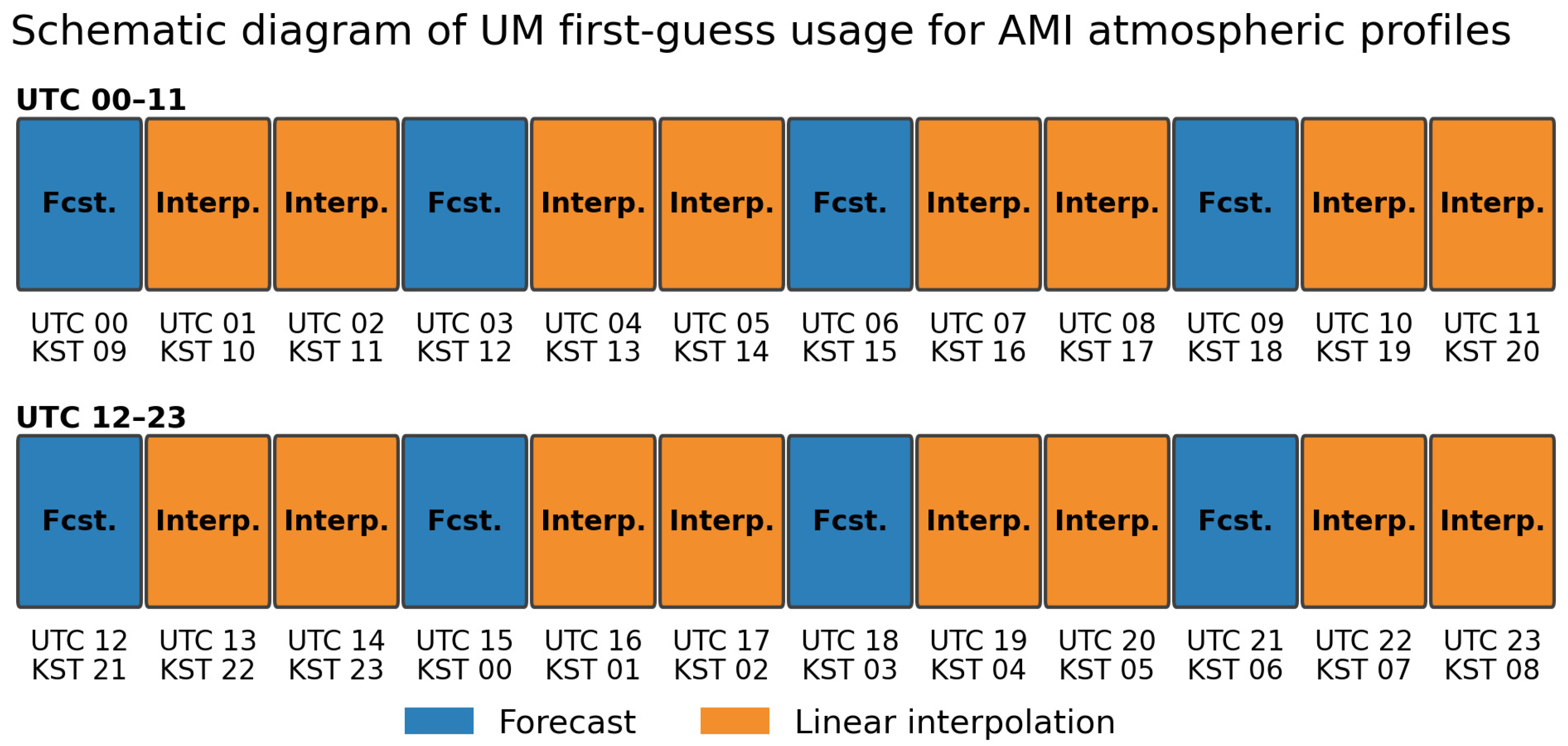
Through an iterative physical retrieval procedure, the AAP algorithm refines temperature and humidity profiles over clear-sky regions by minimizing the difference between observed AMI TBs and TBs simulated using the Radiative Transfer for TOVS (RTTOV) model. Profile retrievals are performed hourly, with UM first-guess profiles temporally interpolated between the nearest forecast times (Figure 1). A detailed description of the AAP algorithm is provided by [4]. The AMI IR channels used in the retrieval are summarized in

Table 1. AMI infrared channels used in the temperature and humidity profile retrieval algorithm. SW, WV, and IR denote shortwave, water vapor, and infrared channels, respectively.

Channel Number	Center Wavelength (µm)	Used in RTTOV	Channel Usage
SW07	3.8	O	Surface temperature, cloud detection
WV08	6.3	O	Upper tropospheric water vapor
WV09	6.9	O	Mid-level water vapor
WV10	7.3	O	Lower tropospheric water vapor
IR11	8.7	O	Surface/window channel, cloud-top properties
IR12	9.6	O	Ozone absorption
IR13	10.5	O	Window channel, surface, and cloud-top temperature
IR14	11.2	O	Window channel, surface, and cloud-top temperature
IR15	12.2	X	Window channel
IR16	13.2	O	CO2 absorption, cloud height estimation

.

2.2. ERA5 Profiles

ERA5 provides hourly global atmospheric fields by combining extensive historical observations with advanced numerical modeling and data assimilation [39]. The dataset is available on a 0.25° × 0.25° grid (approximately 31 km at the equator) and resolves the atmosphere using 37 pressure levels spanning 1000–1 hPa.

Owing to its comprehensive observational constraints and improved representation of atmospheric circulation relative to earlier reanalysis, ERA5 is widely used as reference data for climate analysis [40], evaluation of operational atmospheric products [41], and the development of ML-based atmospheric models [42]. In this study, ERA5 temperature, mixing ratio, and relative humidity profiles were used as reference data for model training and evaluation.

2.3. Radiosonde (RAOB) Profiles

RAOBs were used as an independent dataset to further evaluate the refined temperature and humidity profiles produced by the LGBM post-processing. We employed quality-controlled radiosonde data from the NOAA Global Systems Laboratory, which undergo systematic gross-error screening and hydrostatic consistency checks [43,44].

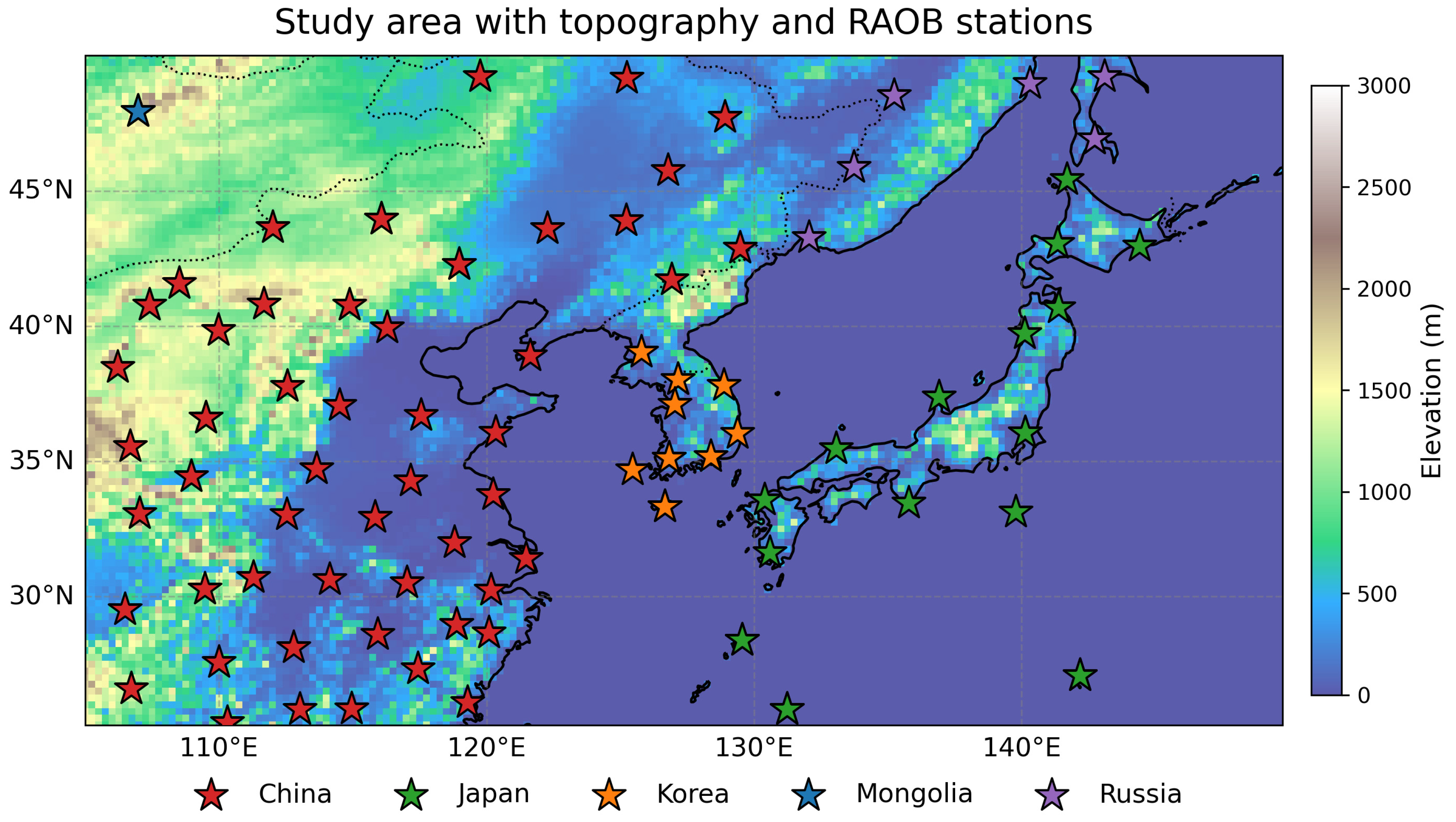
RAOBs are typically launched twice daily (00 and 12 UTC) and provide high-vertical-resolution atmospheric profiles. For this study, RAOB data over East Asia from 2020 to 2023 were collected, and station locations are shown in Figure 2. Because RAOB records provide air temperature and dew-point temperature rather than humidity directly, mixing ratio (Q) and relative humidity (RH) were derived using the following relationships:

$$e_s\left(T\right)=6.112\mathrm{e}\mathrm{x}\mathrm{p}\left({\displaystyle \frac{17.67(T-273.15)}{T-29.65}}\right)$$

(1)

$$RH={\displaystyle \frac{e_s\left(T_{dew}\right)}{e_s\left(T_{air}\right)}}$$

(2)

$$Q=\epsilon {\displaystyle \frac{e}{p-e}}$$

(3)

where $T_{air}$ is the observed ambient air temperature and $T_{dew}$ is the corresponding dew-point temperature at each pressure level, $e_s$ for saturation vapor pressure, $\epsilon$ is the ratio of molecular weights of water vapor to dry air (~0.622), $e$ is vapor pressure, and $p$ is total pressure [45]. Profiles from RAOBs were not used during the training phase, but were used only for the evaluation. The national distribution of RAOBs is provided in Table S1, while the monthly distribution is shown in Table S2. Detailed descriptions of RAOBs across different years, seasons, cloud conditions, land cover types, and major pressure levels are presented in Table S3.

2.4. Auxiliary Input Data

Because cloud contamination strongly affects IR radiance and atmospheric profile retrievals, the AMI cloud mask was incorporated as an input feature. A land–sea mask from AMI was also used to account for differences in surface radiative characteristics between land and ocean. To represent topographic influences on near-surface atmospheric structure, a 2 km global DEM derived from the Multi-Error-Removed Improved-Terrain (MERIT) DEM was included [46,47].

The specifications of all datasets used in this study are summarized in

Table 2. Specifications of datasets used in this study. The spatial resolution indicates horizontal grid spacing, and the temporal resolution shows the original data frequency. Note that although GK2A TB measurements are available at a higher temporal frequency of 10 min, we only used hourly (top of the hour) data to maintain temporal consistency with AMI and ERA5 profiles. T, Q, and RH stand for temperature, mixing ratio, and relative humidity, respectively.

Variable	Source	Spatial Resolution	Temporal Resolution	Unit	Usage
T, Q, RH profile	GK2A (NMSC, KMA)	6 km	1 h	K, g/kg, %	Predictor
TB 7-16		2 km	10 min	K
Cloud mask		6 km	1 h	-
Land mask		6 km	-	-
DEM	MERIT DEM	2 km	-	m
T, Q, RH profile	ERA5 (ECMWF)	0.25°	1 h	K, g/kg, %	Target, Evaluation
T, Q, RH profile	RAOB (NOAA)	Point	00, 12 UTC	K, g/kg, %	Evaluation

. Although AMI TB observations are available every 10 min, only hourly data were used to maintain temporal consistency with AMI profile products and ERA5.

3. Methodology

3.1. Data Preprocessing

To ensure consistency across data sources, vertical profile matching between ERA5 and GK2A AMI was first performed using spline interpolation. Only AMI pressure levels that aligned with ERA5 were retained, resulting in a total of 27 common pressure levels spanning 1000–100 hPa.

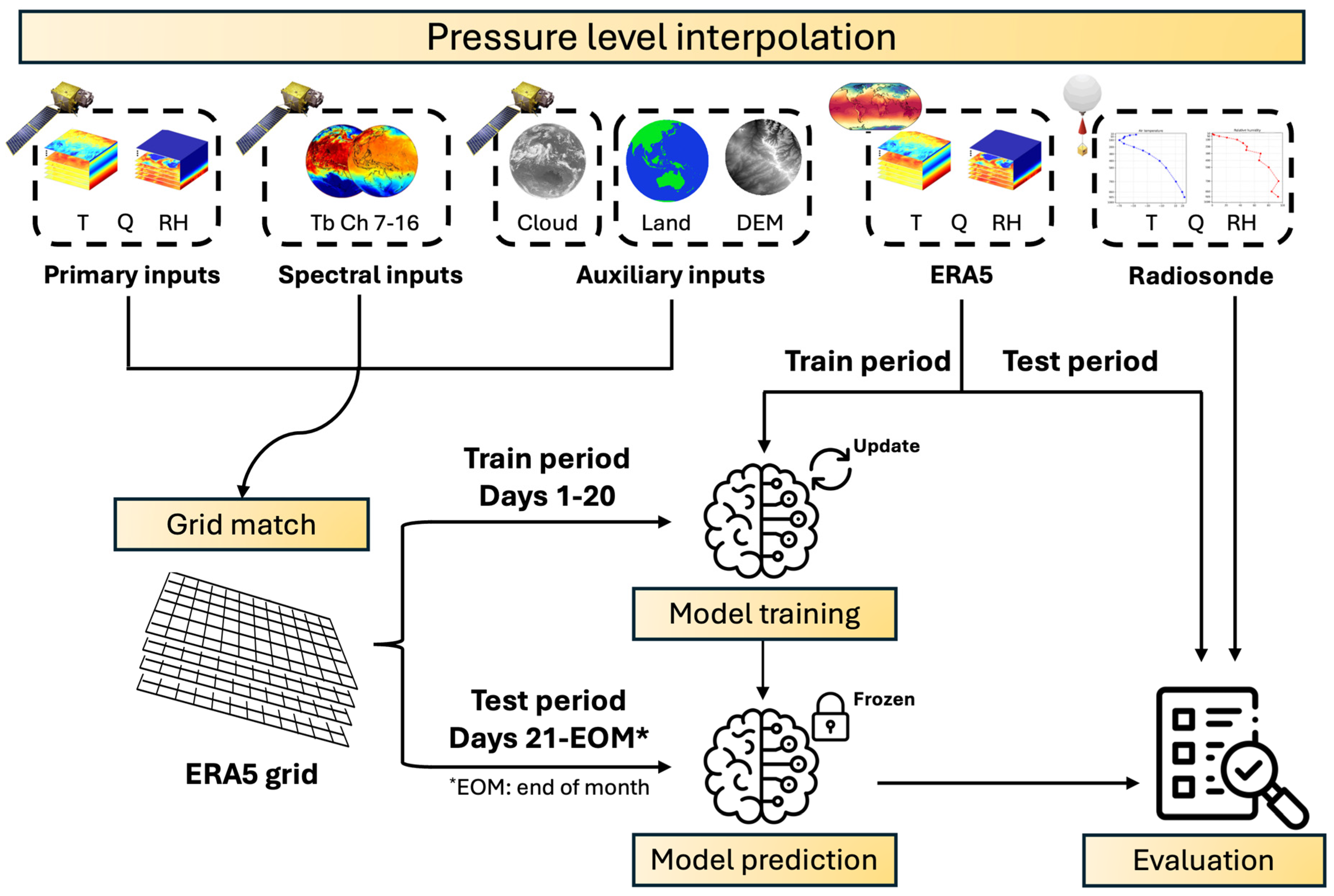
All input variables were then regridded to the ERA5 horizontal grid, which has a coarser spatial resolution and therefore served as the common reference grid (Figure 3). Horizontal interpolation was performed using bilinear interpolation, enabling the extraction of spatially collocated training samples from ERA5 grid cells.

3.2. Sampling and Model Training

ERA5 profiles were temporally partitioned on a monthly basis, with data from the 1st to the 20th day of each month used for training and data from the 21st day to the end of the month reserved for testing (Figure 3). This scheme allows model performance to be evaluated under diverse spatial and temporal conditions within each month, while maintaining a balanced separation between training and evaluation data.

Sampling was performed at hourly (top of the hour) intervals to fully exploit the high temporal resolution of ERA5. This approach enables the model to learn diurnal variations in atmospheric profiles, which are difficult to capture using radiosonde observations alone due to their typical 6–12 h launch intervals. For each hourly timestamp, 2000 randomly selected grid points across the ERA5 domain were sampled. At each location, AMI temperature and humidity profiles, infrared TB, cloud and land masks, and DEM values were collocated with the corresponding ERA5 profiles at each pressure level. This procedure yielded approximately 46 million training samples per variable per pressure level (2000 grid points × 24 h × ~20 training days × 48 months), and approximately 23 million test samples per variable per pressure level (days 21 to month-end over the same 48-month period).

Profile refinement was performed using the LGBM, selected for its computational efficiency, low memory requirements, and strong performance on tabular datasets [48]. LGBM is a gradient boosting framework that iteratively builds an ensemble of decision trees, where each successive tree is trained to correct the residual errors of the previous ensemble. To optimize both accuracy and training speed on large-scale datasets, the algorithm employs histogram-based continuous feature binning and a leaf-wise (best-first) tree growth strategy, which substantially reduces computational cost compared to traditional level-wise growth alternatives. For this study, the key hyperparameters were configured to accommodate the massive dataset while preventing overfitting: maximum number of leaves per tree (num_leaves = 1024), learning rate (0.05), number of boosting iterations (n_estimators = 500), minimum number of samples in a leaf (min_data_in_leaf = 5000), and a feature subsampling ratio (feature_fraction = 0.8) to enhance ensemble robustness. To account for the distinct thermodynamic characteristics at different altitudes, a separate LGBM model was trained for each target variable and pressure level. In total, 81 independent models were developed, covering three variables (temperature T, mixing ratio Q, and relative humidity RH) across 27 pressure levels. This design allows refinement to be optimized independently at each vertical layer.

3.3. Evaluation

As the purpose of this study is to post-process toward reanalysis-consistent results, primary evaluation was conducted using ERA5 data from the withheld test period to assess the model’s ability to reproduce ERA5 profiles under unseen conditions. As an independent benchmark, refined profiles were also compared against RAOBs. While ERA5 assimilates RAOB measurements during reanalysis, the two datasets are not identical due to differences in spatial representativeness, background model physics, and assimilation or quality control procedures. Therefore, refinement relative to ERA5 does not guarantee improved agreement with RAOBs. Comparing the refined profiles against RAOBs serves as a necessary independent test to evaluate whether the data-driven refinement translates into robust physical consistency across different observation types.

Performance was quantified using mean bias and root mean squared error (RMSE), defined as:

$$meanbias={\displaystyle \frac{1}{n}}{\sum }_{i=1}^n({\widehat{y}}_i-y_i)$$

(4)

$$RMSE=\sqrt{{\displaystyle \frac{1}{n}}{\sum }_{i=1}^n{\left({\widehat{y}}_i-y_i\right)}^2}$$

(5)

where $n$ represents the number of samples, and ${\widehat{y}}_i$ and $y_i$ are prediction and reference values for $i$–th pixel, respectively.

3.4. Feature Importance Analysis

To examine the contribution of individual predictors, Shapley Additive Explanations (SHAP) were applied to each LGBM model. SHAP is a widely used explainable ML framework that attributes model predictions to input features based on cooperative game theory [49]. It provides both global and local interpretability by decomposing predictions into additive feature contributions.

In this study, SHAP summary statistics were used to evaluate feature importance for each variable and pressure level. This analysis enables identification of the key predictors driving profile refinement and provides insight into how satellite observations, background profiles, and auxiliary inputs contribute across different vertical layers.

4. Results

4.1. Quantitative Evaluation Under Clear-Sky and Cloudy Conditions

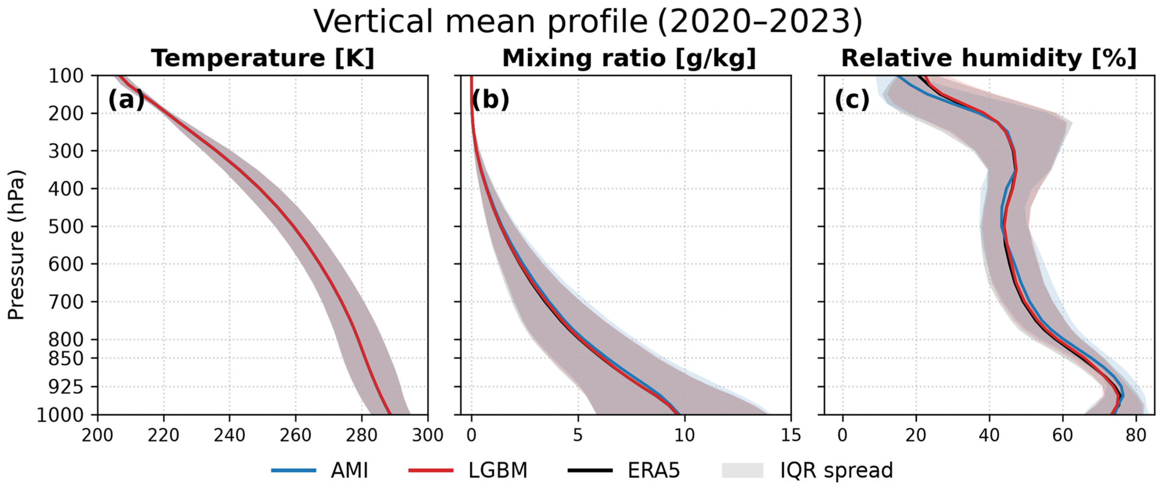
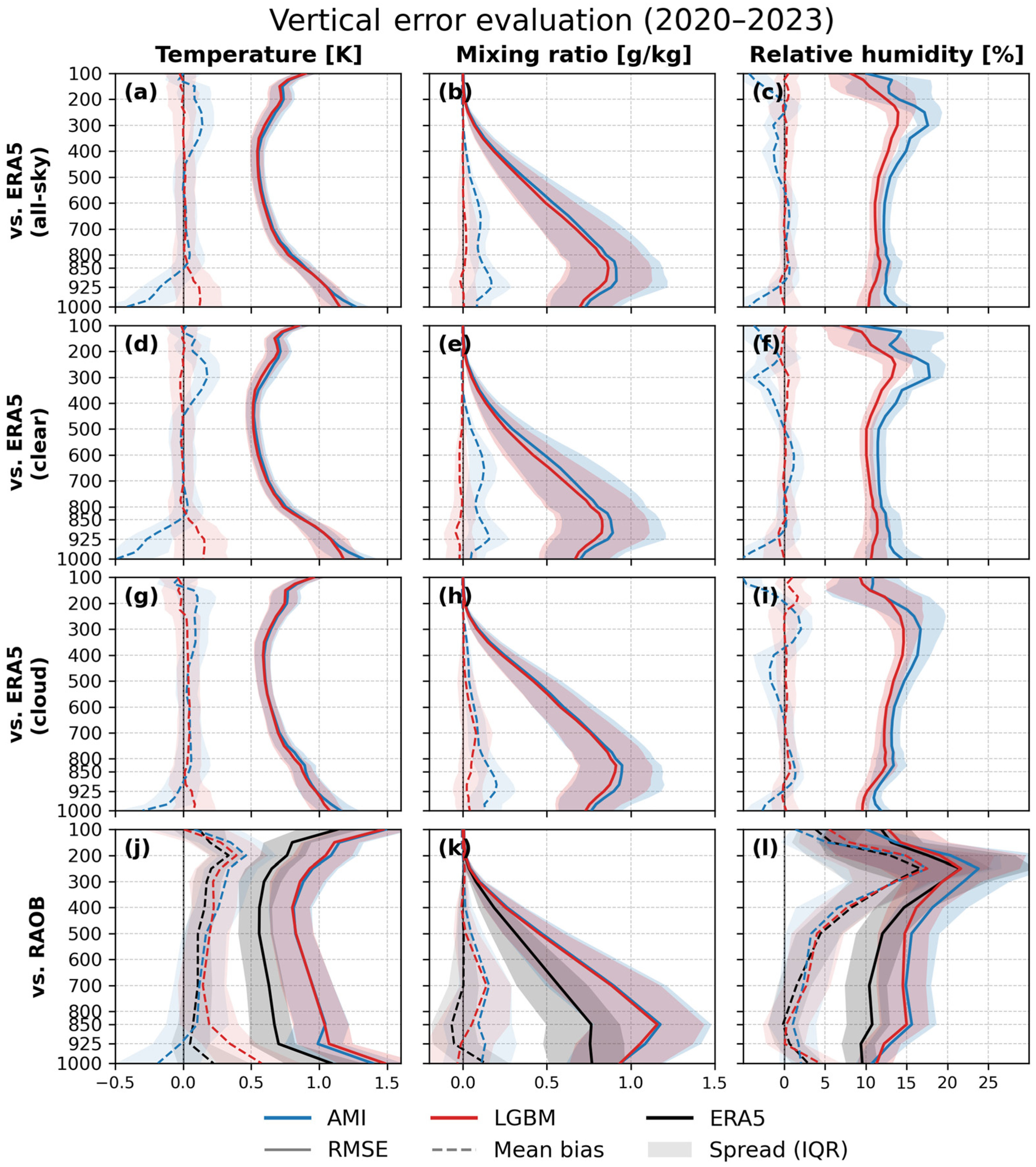
Figure 4 shows vertical mean profiles of temperature, mixing ratio, and relative humidity for 2020–2023. Figure 5 presents the mean bias and RMSE of temperature, mixing ratio, and relative humidity profiles for the period 2020–2023, evaluated against both ERA5 and RAOB observations.

Table 3. RMSE relative to ERA5, aggregated over different pressure layers.

		T (K)			Q (g/kg)			RH (%)
Layer (hPa)	Results	All	Clear	Cloud	All	Clear	Cloud	All	Clear	Cloud
100–300	AMI	0.74	0.71	0.77	0.05	0.04	0.05	15.62	15.99	15.01
	LGBM	0.72	0.69	0.76	0.04	0.03	0.05	12.84	12.31	13.50
300–500	AMI	0.58	0.56	0.62	0.26	0.21	0.31	15.15	14.30	16.25
	LGBM	0.57	0.54	0.61	0.24	0.19	0.29	12.80	11.57	14.39
500–850	AMI	0.69	0.66	0.74	0.72	0.69	0.77	12.59	11.84	13.73
	LGBM	0.68	0.64	0.72	0.68	0.63	0.75	11.44	10.56	12.69
850–1000	AMI	1.08	1.12	1.02	0.91	0.89	0.93	13.02	13.64	11.89
	LGBM	1.05	1.09	0.99	0.85	0.83	0.87	11.09	11.34	10.65
All	AMI	0.77	0.76	0.78	0.60	0.57	0.63	13.87	13.62	14.23
	LGBM	0.75	0.74	0.77	0.56	0.53	0.60	11.96	11.29	12.88

summarizes the RMSE relative to ERA5 across five vertical layers: surface–lower (1000–850 hPa), lower–middle (850–500 hPa), middle–upper (500–300 hPa), upper levels (above 300 hPa), and all levels combined.

When evaluated against ERA5, the LGBM-based refinement yields a modest but consistent reduction in temperature RMSE across most layers. The overall RMSE decreases by approximately 0.02 K, corresponding to a 2–3% closer alignment with ERA5, and this trend is generally consistent under both clear-sky and cloudy conditions (Figure 5a,d,g; Table 3). RMSE values are typically lower under clear-sky conditions than under cloudy conditions by roughly 0.03 K, except near the surface (Figure 5d,g). In terms of systematic error, the refined LGBM profiles show a clearer reduction in mean bias across most vertical layers. In contrast, evaluation against RAOBs clearly shows that the temperature profiles do not benefit from this refinement. Rather, the layer-averaged RMSE slightly degrades by approximately 0.01 K (Figure 5j;

Table 4. Mean bias and RMSE relative to RAOBs, aggregated over different pressure layers.

		T (K)		Q (g/kg)		RH (%)
Layer (hPa)	Results	Bias	RMSE	Bias	RMSE	Bias	RMSE
100–300	AMI	0.31	1.20	0.00	0.06	10.53	22.61
	LGBM	0.23	1.18	0.00	0.06	11.88	21.18
	ERA5	0.21	0.89	0.00	0.05	10.54	21.13
300–500	AMI	0.25	0.89	0.02	0.37	7.90	20.02
	LGBM	0.21	0.88	0.01	0.36	8.42	17.88
	ERA5	0.15	0.62	0.00	0.26	8.70	16.84
500–850	AMI	0.13	0.98	0.10	0.98	2.33	16.22
	LGBM	0.18	0.98	0.07	0.95	2.52	15.46
	ERA5	0.10	0.67	−0.02	0.64	2.15	11.96
850–1000	AMI	−0.03	1.22	0.11	1.18	1.62	13.87
	LGBM	0.37	1.28	0.00	1.16	1.58	13.50
	ERA5	0.12	0.92	0.01	0.84	1.15	10.57
All	AMI	0.16	1.08	0.07	0.80	5.14	18.13
	LGBM	0.24	1.09	0.03	0.78	5.74	17.01
	ERA5	0.14	0.78	0.00	0.55	5.17	15.25

).

For humidity, both mixing ratio and relative humidity exhibit clearer improvements. Mixing ratio RMSE relative to ERA5 decreases by about 0.04 g kg⁻¹ (approximately 6.7%) across all pressure levels (Figure 5b), whereas the improvement relative to RAOBs is smaller (~0.02 g kg⁻¹, ~2.5%; Figure 5j). Relative humidity shows the most pronounced improvement, with an overall RMSE reduction of approximately 6.2% across all pressure levels (Table 4). Given that the original AMI RH profiles already represent an improvement over the UM first guess, the additional refinement achieved by LGBM is notable, corresponding to further reductions of 1.9 percentage points (≈13.8%) relative to ERA5 and 1.12 percentage points (≈6.1%) relative to RAOBs. A sharp change in RH behavior near 200 hPa (Figure 5l) likely reflects increased uncertainty under very dry upper-tropospheric conditions [50]. Because relative humidity can become unstable or physically less meaningful at very low mixing ratios, small absolute errors in moisture can translate into disproportionately large RH differences. Therefore, any statistical improvements or degradations in upper-level RH above about 200 hPa must be interpreted with caution.

4.2. Temporal Consistency and Statistical Significance of Results

The results presented in Section 4.1 represent aggregated statistics over the full 2020–2023 period. To assess whether these error reductions reflect stable generalization over different years, we examine the year-by-year decomposition of layer-averaged ΔRMSE. Tables S4 and S5 provide year-by-year ΔRMSE for ERA5-based and RAOB-based evaluations, respectively. Against ERA5 (Table S4), the temperature RMSE reduction is consistent across all four years, ranging from −2.3% (2023) to −4.1% (2020) at the all-layer level, with no year showing degradation. RMSE reductions for mixing ratio and relative humidity are similarly stable, with all-layer ΔRMSE% ranging from −5.2% to −6.6% for Q and from −13.6% to −14.0% for RH across years. Against RAOBs (Table S5), the lower-tropospheric temperature degradation is also consistent across all four years (+3.4% to +6.9%), confirming that this is a systematic behavior of the post-processing rather than an artifact of a particular year. This trend would not be expected if the model were exploiting within-month climatological patterns specific to the training period.

To further validate the reliability of the model and account for temporal autocorrelation, we applied a monthly block bootstrap resampling approach (2000 replicates; 48 monthly blocks spanning 2020–2023) to estimate 95% confidence intervals (CIs). These CIs are reported for layer-averaged ΔRMSE values in Tables S6 (vs. ERA5) and S7 (vs. RAOBs). Against ERA5, all ΔRMSE values represent statistically significant reductions in RMSE at the 95% level across all layers and variables, as their CIs are entirely negative. Against RAOBs, the overall temperature change (+0.002 K; 95% CI [−0.011, +0.009]) is not statistically significant, whereas the lower-tropospheric (850–1000 hPa) temperature degradation (+0.062 K; 95% CI [+0.032, +0.083]) is statistically significant. RMSE reductions for mixing ratio and relative humidity remain statistically significant at all layers against both ERA5 and RAOBs.

4.3. Seasonal and Diurnal Variability Relative to ERA5

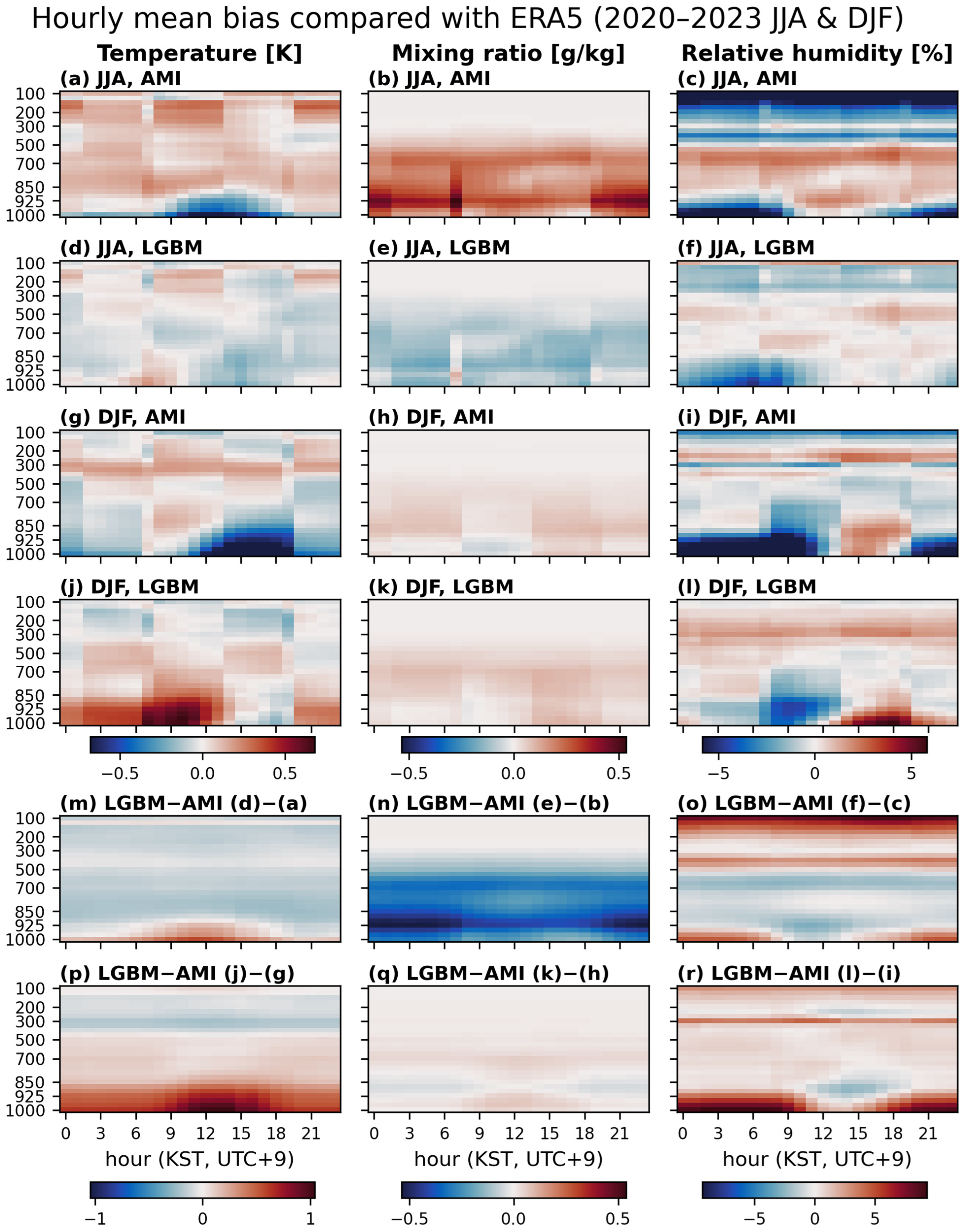
Seasonal and diurnal variations were examined by comparing AMI and LGBM profiles with ERA5 during summer (June–August, JJA) and winter (December–February, DJF) over 2020–2023. Figure 6 shows the hourly mean bias of temperature, mixing ratio, and relative humidity across pressure levels and local time (KST).

AMI exhibits a pronounced diurnal cold bias in temperature below 850 hPa between approximately 09–18 KST during both JJA and DJF (Figure 6a,g). LGBM substantially reduces this bias during JJA but introduces a warm bias in DJF, particularly near the surface during the overnight and morning hours (approximately 20–14 KST). This behavior is consistent with the near-surface bias patterns identified in Figure 5. Difference plots (Figure 6m–r) highlight how LGBM modifies the AMI temperature bias, revealing a persistent warm bias below about 500 hPa in DJF.

For the mixing ratio, AMI shows a strong positive bias during JJA (Figure 6b), which is effectively reduced by LGBM, resulting in a slightly negative bias (Figure 6e). In DJF, both AMI and LGBM exhibit smaller and slightly positive biases. Relative humidity displays distinct diurnal structures near the surface (Figure 6c,f,i,l), closely linked to the combined behavior of temperature and moisture.

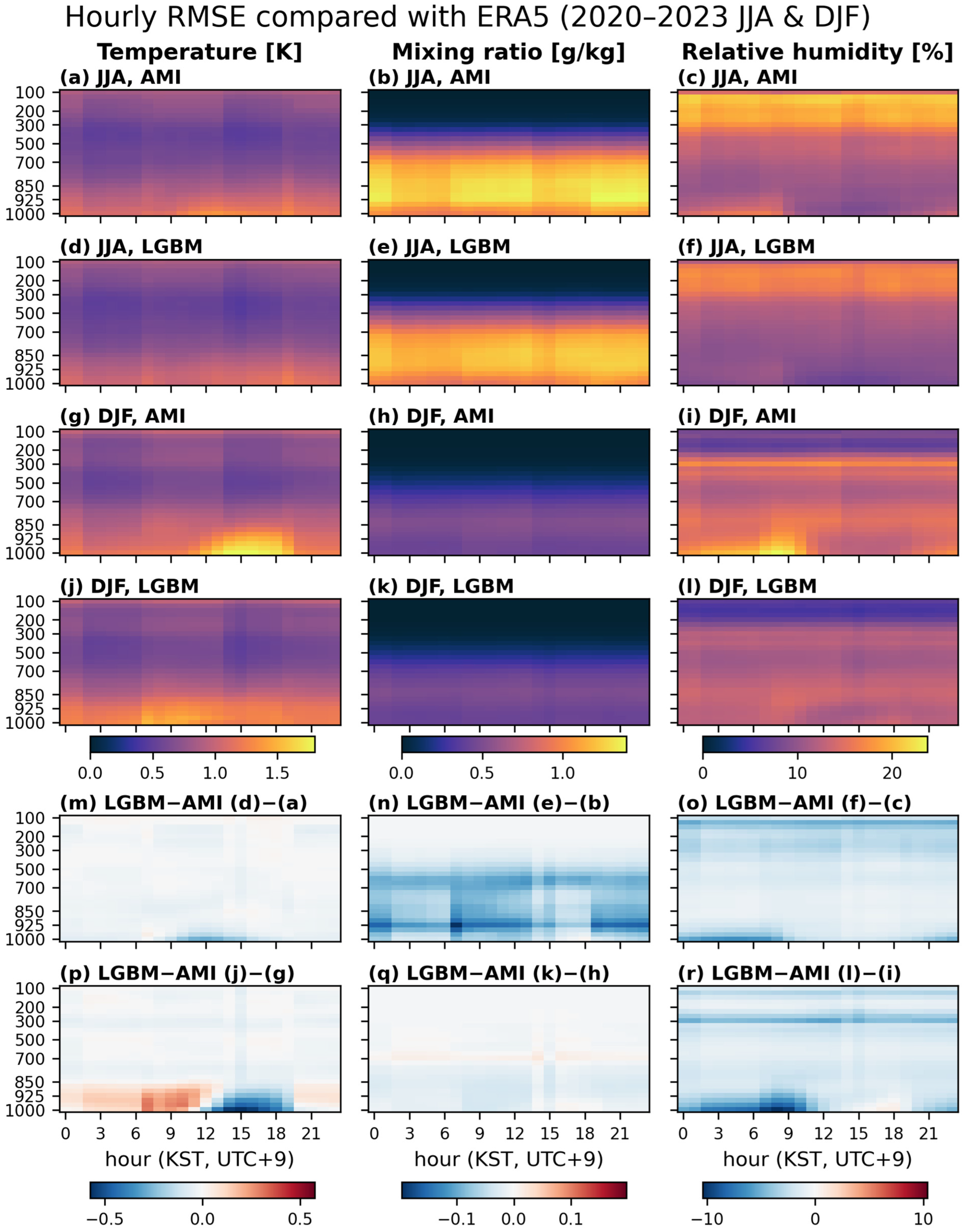
RMSE patterns (Figure 7) show increased temperature RMSE near the surface between approximately 12–18 KST for AMI (Figure 7g), likely reflecting enhanced diurnal variability in boundary-layer conditions [51,52]. Mixing ratio RMSE exhibits strong seasonal contrasts, with larger errors in summer below about 400 hPa (Figure 7b) and smaller errors in winter (Figure 7e), consistent with seasonal water vapor distributions. LGBM reduces temperature RMSE below about 850 hPa during daytime in JJA (Figure 7m,p) but increases RMSE during nighttime and morning hours in DJF. For mixing ratio and relative humidity, LGBM generally yields consistent RMSE reductions across seasons.

Across all three variables, distinct diurnal RMSE structures are evident around 02–06 KST and 14–18 KST (23–03 UTC and 11–15 UTC). These patterns may partly originate from varying lead times and linear temporal interpolation of UM first-guess profiles (Figure 1), although further investigation is required to isolate their causes.

4.4. Seasonal and Spatial Evaluation Relative to RAOBs

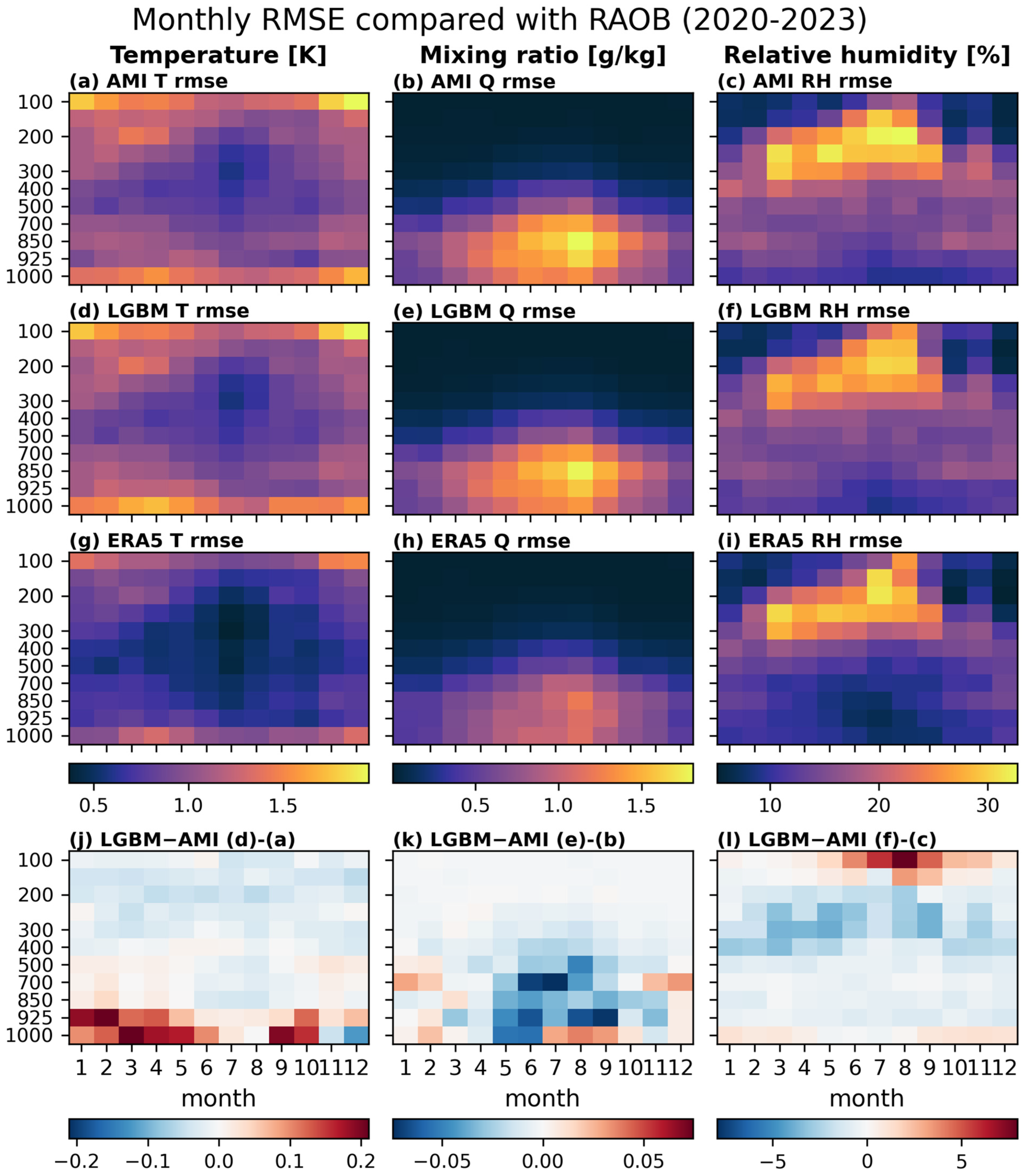
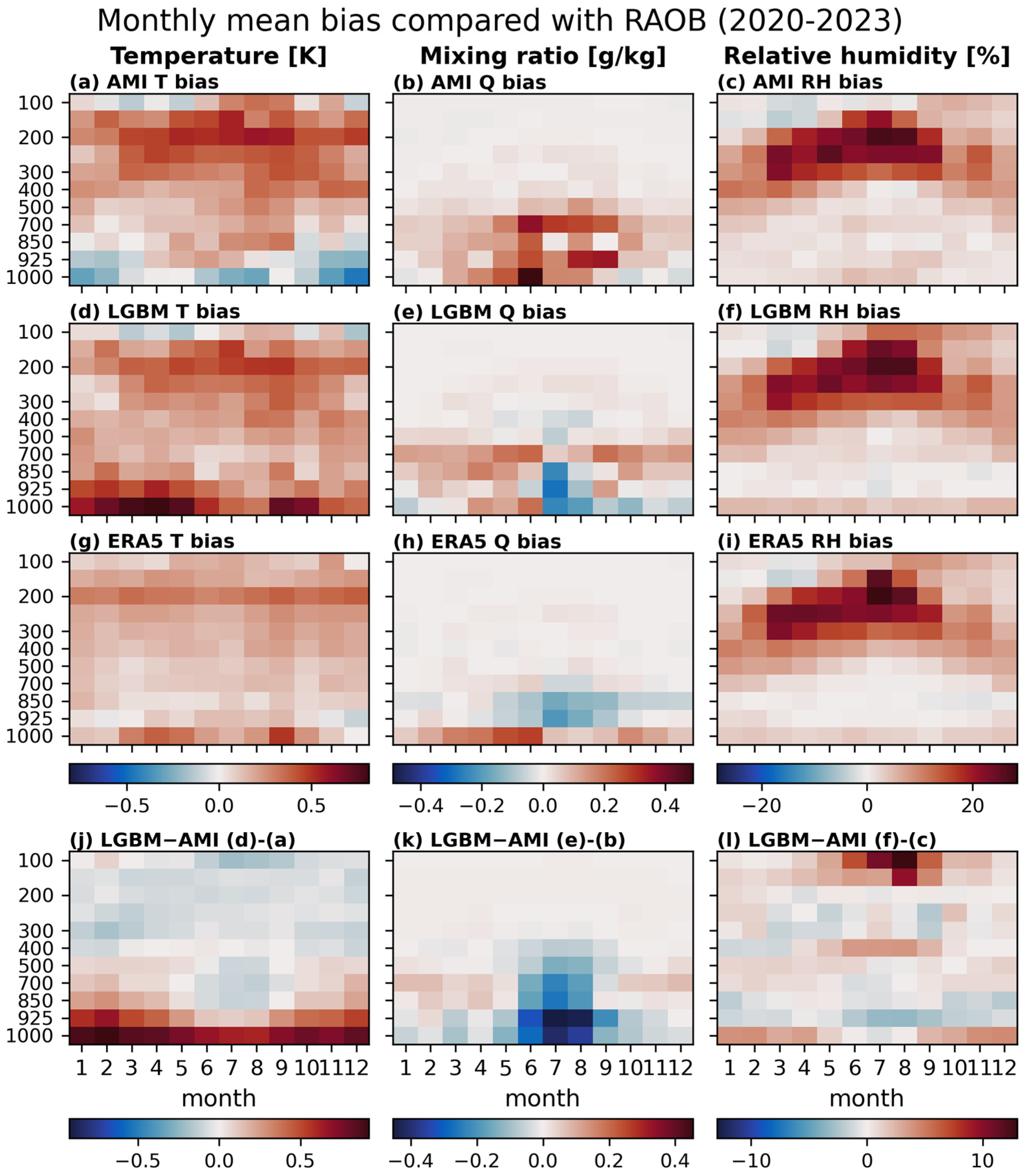
Figure 8 and Figure 9 show monthly mean bias and RMSE of temperature, mixing ratio, and relative humidity profiles from AMI, LGBM, and ERA5 relative to RAOBs for 2020–2023. All three datasets exhibit similar seasonal bias patterns, with generally positive biases relative to RAOBs. A notable feature is the large RH bias in the upper troposphere between March and September (Figure 8c,f,i), likely reflecting high uncertainty under very dry conditions aloft.

ERA5 consistently shows lower RMSE than both AMI and LGBM across all pressure levels (Figure 9g–i). LGBM exhibits increased temperature RMSE below about 850 hPa (Figure 9d), as also indicated in Table 4. The smaller RMSE increase during JJA may be related to the overall reduction in RMSE relative to ERA5 (Figure 7), suggesting that improvements relative to ERA5 can, in some cases, translate into improvements relative to RAOBs. Previous studies report near-surface temperature RMSE of AMI relative to RAOBs in the range of ~0.4–1.0 K, depending on region and radiosonde type [4,25], indicating that further work is needed to distinguish model-related effects from representativeness and observational uncertainties.

For the mixing ratio, LGBM shows a clear RMSE reduction during JJA (Figure 9k), consistent with the ERA5-based results. The sharp increase in RH RMSE above ~200 hPa (Figure 9c,f,i) likely reflects the limited reliability of radiosonde humidity measurements at very low mixing ratios [53].

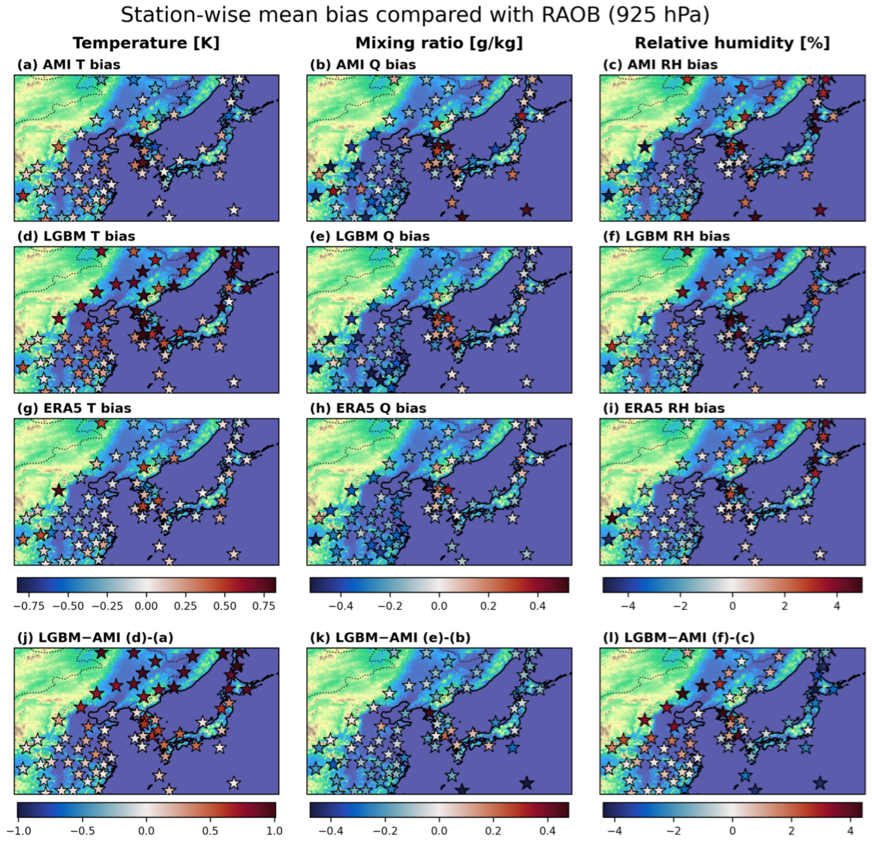
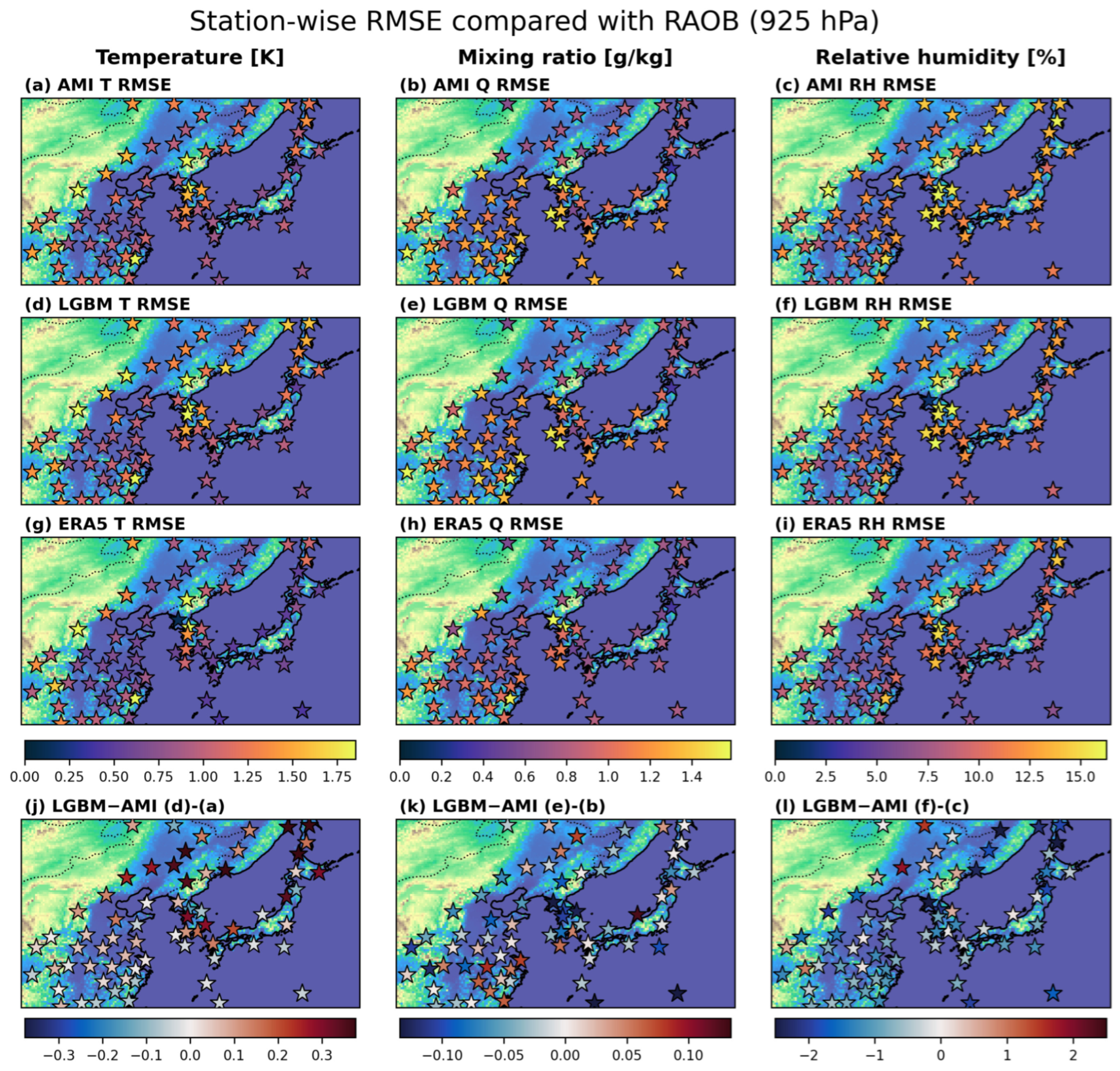
To further examine low-level spatial performance—where large biases in both temperature (T) and mixing ratio (Q) are evident between AMI and LGBM (Figure 8j,k)—we analyzed station-wise mean bias and RMSE at 925 hPa across East Asia (Figure 10 and Figure 11). AMI exhibits a broadly positive temperature bias over most of Korea, China, and Japan (Figure 10a). In contrast, LGBM introduces a positive temperature bias in regions where AMI shows a negative bias relative to RAOBs, most notably over Russia (Figure 10d,j). This likely reflects an over-correction of the near-surface cold bias in AMI, consistent with the diurnal patterns shown in Figure 6a,m. Many of the affected stations are located at relatively high elevations, which may further contribute to this behavior. A similar spatial structure is evident in the RMSE differences for temperature (Figure 11j).

For both Q and relative humidity (RH), LGBM generally reduces the positive bias of the original AMI profiles at 925 hPa, particularly over Japan and adjacent oceanic regions (Figure 10k,l), and these improvements are also reflected in the RMSE differences (Figure 11k,l). However, some inland stations show increased RMSE in Q and RH, indicating that refinement performance is spatially heterogeneous near the surface.

4.5. Application to TPW and CAPE

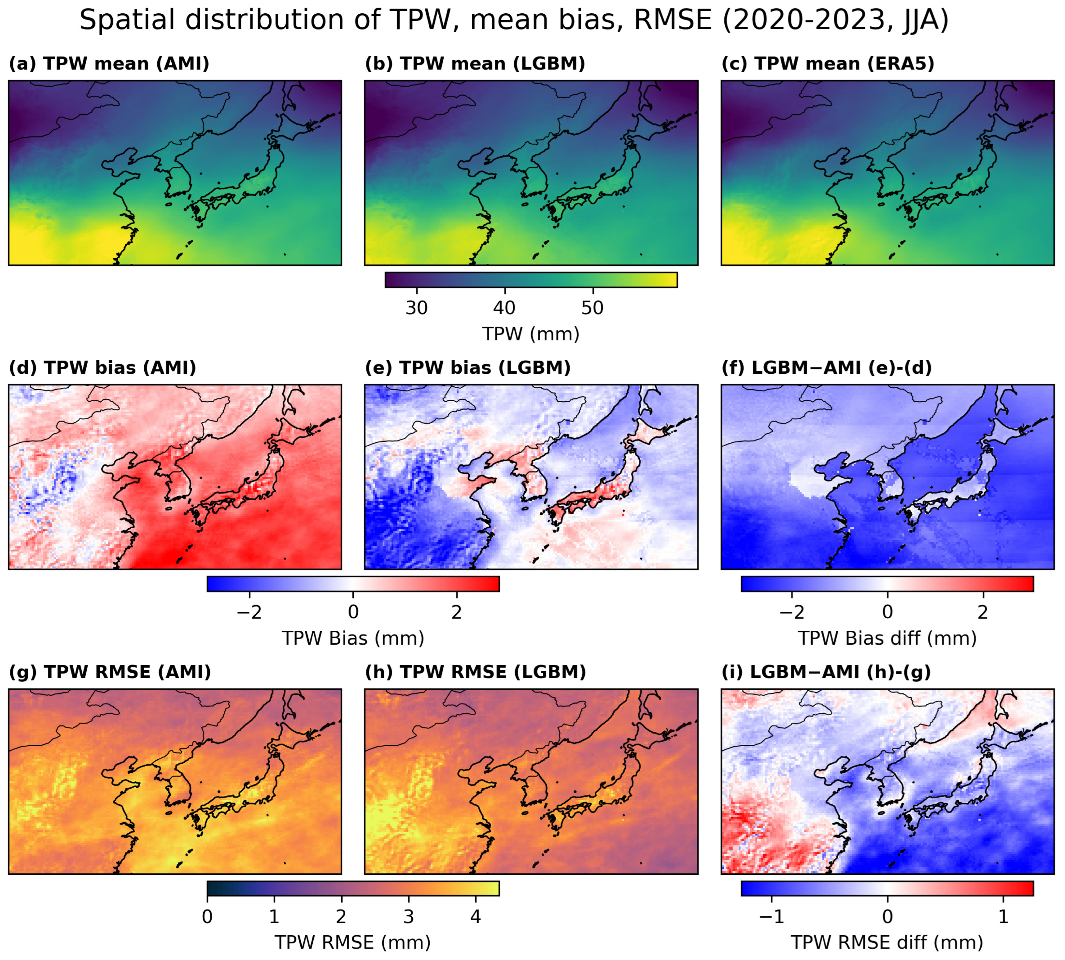
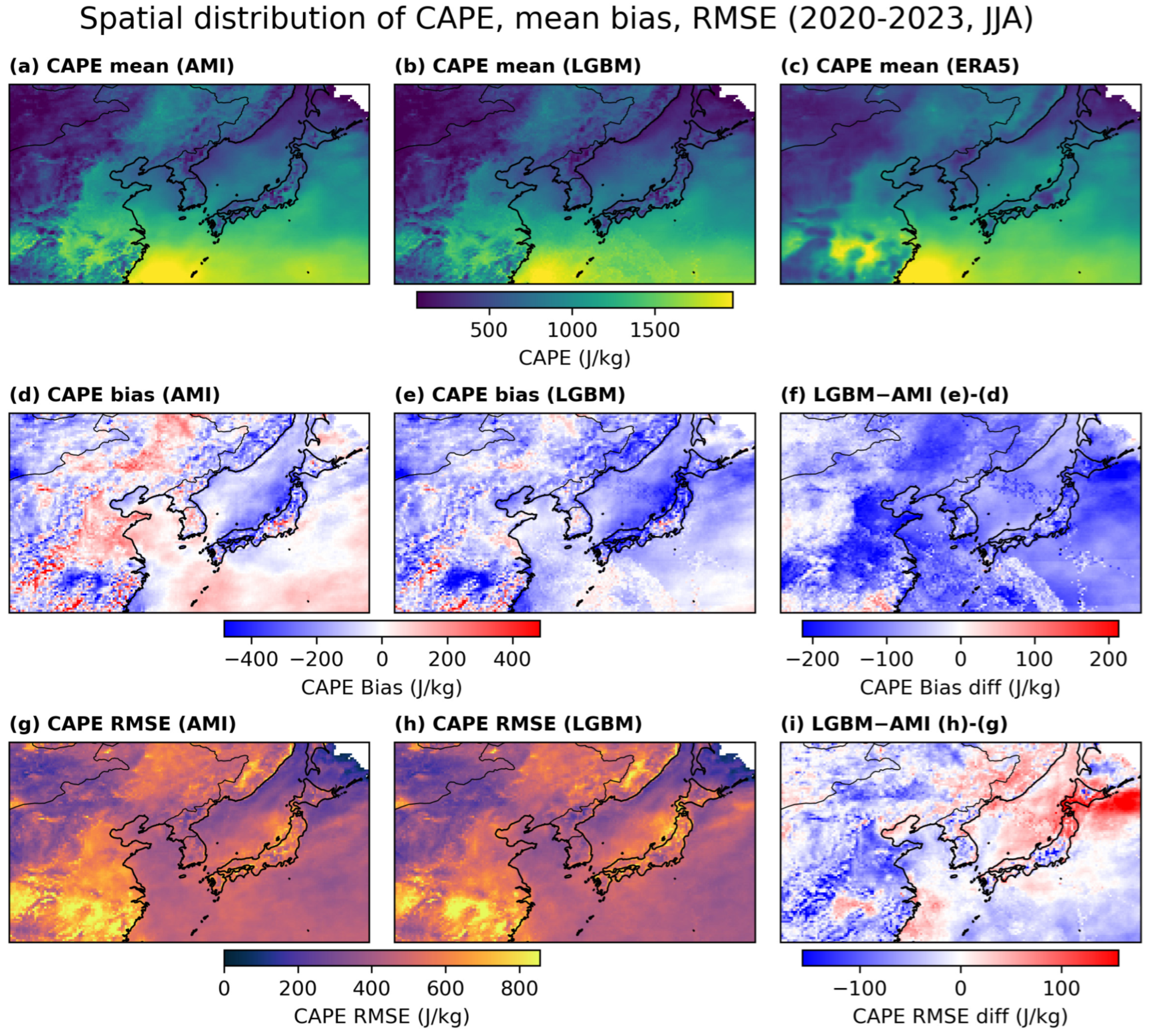
To assess the practical implications of profile refinement, hourly TPW and CAPE were derived from the refined profiles during JJA, when moisture and convective instability are highest over East Asia. Figure 12 and Figure 13 present spatial distributions of mean values, biases, and RMSE relative to ERA5, and

Table 5. Summary of mean bias and RMSE for TPW relative to ERA5 during 2020–2023 JJA (mm).

	Profile	Mean Bias	RMSE
All	AMI	1.12	3.16
	LGBM	−0.57	2.89
Land	AMI	0.92	3.30
	LGBM	−0.80	3.10
Ocean	AMI	1.35	3.00
	LGBM	−0.29	2.64

and

Table 6. Summary of mean bias and RMSE for TPW and CAPE compared with ERA5 during 2020–2023 JJA (J kg⁻¹).

	Profile	Mean Bias	RMSE
All	AMI	−37.91	465.74
	LGBM	−133.97	454.86
Land	AMI	−34.93	490.33
	LGBM	−121.05	465.31
Ocean	AMI	−41.54	435.85
	LGBM	−149.69	442.17

summarize statistics over land and ocean.

For TPW, all datasets reproduce the expected spatial patterns over East Asia (Figure 12a–c). AMI tends to overestimate TPW by 1–2 mm, particularly over oceanic regions, whereas LGBM generally reduces this bias. Some inland regions show slight negative biases, suggesting partial over-correction. RMSE maps and summary statistics confirm that LGBM reduces TPW errors relative to AMI, consistent with the ~5–6% reduction in mixing ratio RMSE below 500 hPa and an overall ~8.5% reduction in TPW RMSE.

For CAPE, values below 100 J kg⁻¹ were excluded to focus on convectively relevant conditions. LGBM reduces CAPE RMSE over most land areas but increases errors over some oceanic regions near northern Japan (Figure 13). This behavior is reflected in Table 6, indicating enhanced consistency over land performance but mixed results over the ocean, along with a more negative overall bias. Because CAPE is highly sensitive to small vertical inconsistencies in low-level profiles, these mixed results suggest that the operational utility of the framework requires further validation through specific weather-diagnosis tasks, such as convective initiation or heavy rainfall cases.

4.6. Vertical Patterns in Feature Importance

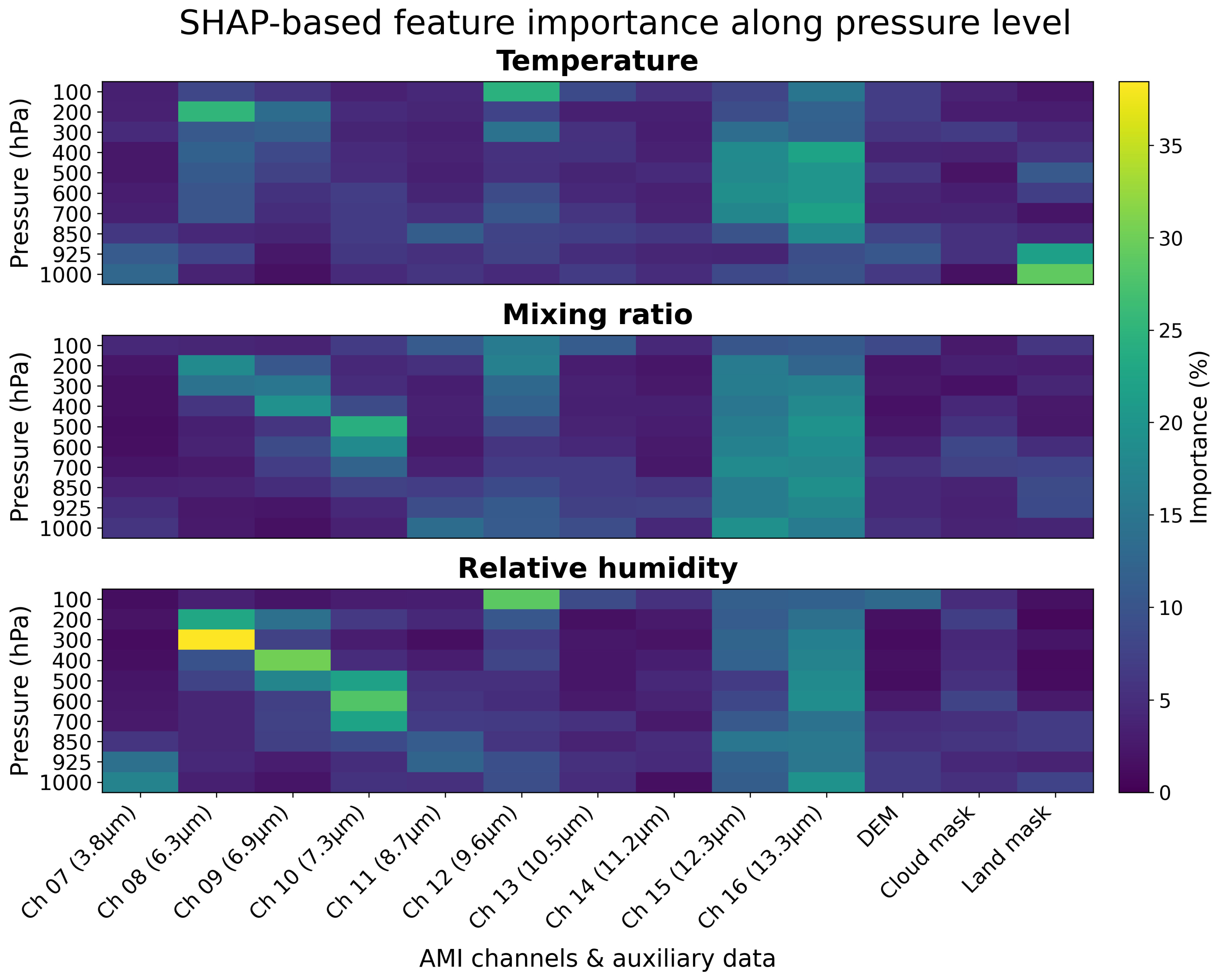
Vertical feature importance derived from SHAP analysis is shown in Figure 14. To emphasize the role of satellite-derived predictors, AMI temperature and humidity profiles at each level were excluded from this analysis. Channel 7 exhibits weak importance near the surface, likely reflecting sensitivity to shortwave surface radiation. Cloud and land masks show enhanced importance near the surface, highlighting their role in modulating near-surface radiative and cloud effects. The DEM contributes primarily to temperature refinement at lower levels.

The most pronounced vertical structure appears in the water vapor channels (Channels 8–10), with peak importance at different layers: Channel 8 near 200–400 hPa, Channel 9 near 300–500 hPa, and Channel 10 near 400–600 hPa. These patterns are consistent with known vertical sensitivity characteristics of water vapor channels in geostationary imagers [54,55]. By contrast, window channels (Channels 13 and 14) show consistently low importance. While these channels are critical for surface and cloud-top estimation in RTM-based retrievals [4], their limited contribution here suggests that much of their information content is already utilized during the physical retrieval stage. Further investigation is required to fully interpret this behavior.

5. Discussion

The long-term evaluation presented in this study highlights both the potential and the inherent limitations of refining geostationary imager–based temperature, mixing ratio, and relative humidity profiles using ML–based residual correction. Overall, the LGBM refinement yields only modest reductions in temperature RMSE (approximately 0.02 K, or 2–3%) when evaluated against ERA5, whereas more pronounced error reductions are observed for moisture-related variables, including mixing ratio (about 0.04 g kg⁻¹, or 6–7%) and relative humidity (around 1.9 percentage points, or ≈14%). When compared with independent radiosonde observations, RMSE shows degradation for temperature (<1% overall, with larger degradation in the lower troposphere), but modest RMSE decrease for mixing ratio (≈2–3%) and relative humidity (≈6–7%). These results suggest that, although systematic biases—particularly in moisture fields—can be reduced, the magnitude of achievable error reduction is constrained by both the quality of the first-guess profiles and the limited radiative sensitivity of AMI infrared channels relative to hyperspectral sounders [4,5,25]. Critically, the negligible temperature improvement against RAOBs is itself an informative finding rather than a failure of the framework: it suggests that the UM first-guess profiles already capture most of the temperature structure present in ERA5, leaving little residual signal for the ML model to learn. In effect, much of the retrievable temperature information has already been extracted during the AAP retrieval through the UM first guess and RTTOV-based physical inversion [4,15,25].

In contrast, mixing ratio and relative humidity benefit more clearly from post-processing, particularly below about 500 hPa and during the summer season, when atmospheric moisture content is high and water-vapor channel sensitivity is strongest. Seasonal and diurnal analyses show that AMI exhibits systematic wet biases during JJA, which propagate into relative humidity and are effectively mitigated by the LGBM refinement. This improvement is reflected in integrated moisture diagnostics such as TPW, where relatively small reductions in lower-tropospheric mixing ratio lead to meaningful bias decreases because most atmospheric water vapor resides below the mid-troposphere. The SHAP analysis supports this interpretation, indicating that the three AMI water-vapor channels (6.3–7.3 µm) dominate the refinement process, with peak importance at pressure levels consistent with their established weighting functions in geostationary imagers [54,55]. Although these feature attributions strongly suggest the utilization of genuine spectral information, formal ablation experiments remain a key priority for future work to quantitatively isolate the impact of satellite radiances from that of pure statistical bias correction.

Nevertheless, improvements relative to RAOBs are generally smaller than those relative to ERA5, particularly for temperature in the lower troposphere, where RMSE sometimes increases slightly. This discrepancy likely reflects a combination of representativeness differences between gridded products and point observations, radiosonde sensor uncertainty, and the fact that the model is trained to align with ERA5 rather than directly with in situ measurements [39,53]. These findings suggest that additional evaluation beyond long-term climatological statistics is needed. Although diagnostics such as TPW and CAPE already show meaningful changes, event-based analyses—such as convective initiation or heavy precipitation cases—would provide clearer insight into whether refined profiles translate into practical operational utility [5].

From a modeling perspective, the current framework refines each pressure level independently. This level-by-level design was intentionally adopted for two reasons: first, it is the simplest interpretable baseline for a post-processing framework, where the first-guess profile is already provided by the UM and AMI considering atmospheric vertical structure; second, it enables fully parallel training and evaluation across 81 models on the large-scale dataset. While this design simplifies learning and allows targeted correction at individual levels, it does not explicitly enforce vertical coherence among temperature, mixing ratio, and relative humidity. Nevertheless, because the models correct systematic departures from an already physically consistent first-guess profile, they do not produce physically arbitrary structures. This is evidenced by the continuous vertical patterns observed in the bias and RMSE profiles (Figure 8 and Figure 9), as well as the systematic variations in feature importance across pressure levels revealed by the SHAP analysis (e.g., for Channels 08–10). These findings suggest that the framework implicitly captures meaningful vertical structures through the shared feature space.

Future work should therefore explore vertically aware learning architectures that explicitly represent three-dimensional atmospheric structure, as well as training strategies that incorporate both reanalysis and radiosonde data so that models converge toward multiple references (e.g., ERA5 and RAOBs). In addition, concepts related to real-time bias correction that integrate surface observations and NWP guidance (e.g., [56]) may further enhance performance near the surface, where land–atmosphere coupling plays a critical role.

6. Conclusions

This study presents a data-driven post-processing framework to refine temperature, mixing ratio, and relative humidity profiles retrieved from the GK2A AMI. For each variable and pressure level, an LGBM model was developed to provide post-processing toward ERA5-consistent profiles using AMI-retrieved profiles, ten infrared TB channels (Channels 7–16), cloud and land masks, and a DEM as inputs. Model training was conducted on an hourly basis from January 2020 to December 2023, using ERA5 as the reference, with data from the 1st–20th days of each month for training and the remaining days for independent testing to minimize temporal overlap.

Evaluation against both ERA5 and RAOBs accounted for cloud conditions as well as seasonal and diurnal variability. Relative to ERA5, the refined profiles show modest but consistent RMSE reductions of approximately 0.02 K for temperature (2–3%), 0.04 g kg⁻¹ for mixing ratio (6–7%), and 1.9 percentage points for relative humidity (≈14%). When evaluated against RAOBs, the temperature RMSE shows overall marginal degradation (~0.01 K, or 0–1%) with a more pronounced increase in the lower troposphere (~5%), indicating that temperature benefits are not robust against independent observations. In contrast, RMSE decreases for mixing ratio (~0.01 g kg⁻¹, or 2–3%) and relative humidity (~1.1 percentage points, or 6–7%), confirming that the framework is primarily effective for humidity refinement. Diurnal analyses reveal systematic error structures in the original AMI profiles that may be related to UM first-guess lead times, while seasonal differences are most pronounced for mixing ratio during summer (JJA).

Feature importance analysis highlights the dominant role of the AMI water vapor channels (Channels 8–10), particularly for refining mixing ratio and relative humidity between roughly 200 and 600 hPa, consistent with their known vertical sensitivity. These profile-level RMSE reductions are also reflected in integrated diagnostics such as TPW and CAPE, where bias and RMSE are generally reduced, especially over oceanic and coastal regions, despite the relatively small magnitude of improvements at individual pressure levels.

Overall, this work explores the feasibility study of reanalysis-consistent post-processing for geostationary imager atmospheric profiles. The results identify systematic seasonal, diurnal, and land–ocean error characteristics and demonstrate that data-driven refinement of RTM-based geostationary retrievals is feasible, while also being fundamentally constrained by the limited information content of current imager spectral configurations and the structure of existing physical retrieval algorithms. These findings establish a realistic benchmark and a foundation for future refinement frameworks that more tightly integrate physical retrievals and ML methods across the vertical dimension. Future research should explore vertically coherent deep learning approaches and real-time evaluation in severe weather applications to further enhance the operational relevance of geostationary atmospheric profile products.

References

1. Ooyama, K.V. A dynamic and thermodynamic foundation for modeling the moist atmosphere with parameterized microphysics. J. Atmos. Sci. 2001, 58, 2073–2102. [Google Scholar] [CrossRef]
2. Brotzge, J.A.; Berchoff, D.; Carlis, D.L.; Carr, F.H.; Carr, R.H.; Gerth, J.J.; Gross, B.D.; Hamill, T.M.; Haupt, S.E.; Jacobs, N.; et al. Challenges and Opportunities in Numerical Weather Prediction. Bull. Am. Meteorol. Soc. 2023, 104, E698–E705. [Google Scholar] [CrossRef]
3. Jun, T.; Rind, D. Increasing contribution of the atmospheric vertical motion to precipitation in a warming climate. Commun. Earth Environ. 2024, 5, 541. [Google Scholar] [CrossRef]
4. Lee, S.J.; Ahn, M.H.; Chung, S.R. Atmospheric profile retrieval algorithm for next generation geostationary satellite of Korea and its application to the advanced Himawari Imager. Remote Sens. 2017, 9, 1294. [Google Scholar] [CrossRef]
5. Schmit, T.J.; Li, J.; Lee, S.J.; Li, Z.; Dworak, R.; Lee, Y.K.; Bowlan, M.; Gerth, J.; Martin, G.D.; Straka, W. Legacy atmospheric profiles and derived products from GOES-16: Validation and applications. Earth Space Sci. 2019, 6, 1730–1748. [Google Scholar] [CrossRef]
6. Haynes, K.; Stock, J.; Dostalek, J.; Anderson, C.; Ebert-Uphoff, I. Exploring the use of machine learning to improve vertical profiles of temperature and moisture. Artif. Intell. Earth Syst. 2024, 3, e220090. [Google Scholar] [CrossRef]
7. Lee, S.J.; Ahn, M.H.; Lee, Y. Application of an artificial neural network for a direct estimation of atmospheric instability from a next-generation imager. Adv. Atmos. Sci. 2016, 33, 221–232. [Google Scholar] [CrossRef]
8. Hu, J.J.; Wu, J.; Petropoulos, G.P.; Bao, Y.S.; Liu, J.; Lu, Q.F.; Wang, F.; Zhang, H.; Liu, H. Temperature and relative humidity profile retrieval from Fengyun-3D/VASS in the Arctic region using neural networks. Remote Sens. 2023, 15, 1648. [Google Scholar] [CrossRef]
9. Luo, Y.Y.; Wu, H.; Gu, T.F.; Wang, Z.L.; Yue, H.Y.; Wu, G.S.; Zhu, L.F.; Pu, D.Y.; Tang, P.; Jiang, M.J. Machine learning model-based retrieval of temperature and relative humidity profiles measured by microwave radiometer. Remote Sens. 2023, 15, 3838. [Google Scholar] [CrossRef]
10. Carminati, F.; Migliorini, S.; Ingleby, B.; Bell, W.; Lawrence, H.; Newman, S.; Hocking, J.; Smith, A. Using reference radiosondes to characterise NWP model uncertainty for improved satellite calibration and validation. Atmos. Meas. Tech. 2019, 12, 83–106. [Google Scholar] [CrossRef]
11. Naakka, T.; Nygård, T.; Tjernström, M.; Vihma, T.; Pirazzini, R.; Brooks, I.M. The impact of radiosounding observations on numerical weather prediction analyses in the Arctic. Geophys. Res. Lett. 2019, 46, 8527–8535. [Google Scholar] [CrossRef]
12. Hagelin, S.; Azad, R.; Lindskog, M.; Schyberg, H.; Körnich, H. Evaluating the use of Aeolus satellite observations in the regional numerical weather prediction (NWP) model Harmonie–Arome. Atmos. Meas. Tech. 2021, 14, 5925–5938. [Google Scholar] [CrossRef]
13. Rojas-Campos, A.; Wittenbrink, M.; Nieters, P.; Schaffernicht, E.J.; Keller, J.D.; Pipa, G. Postprocessing of NWP precipitation forecasts using deep learning. Weather Forecast. 2023, 38, 487–497. [Google Scholar] [CrossRef]
14. Menzel, W.P.; Holt, F.C.; Schmit, T.J.; Aune, R.M.; Schreiner, A.J.; Wade, G.S.; Gray, D.G. Application of GOES-8/9 soundings to weather forecasting and nowcasting. Bull. Am. Meteorol. Soc. 1998, 79, 2059–2078. [Google Scholar] [CrossRef]
15. Li, Z.L.; Li, J.; Menzel, W.P.; Schmit, T.J.; Nelson, J.P.; Daniels, J.; Ackerman, S.A. GOES sounding improvement and applications to severe storm nowcasting. Geophys. Res. Lett. 2008, 35. [Google Scholar] [CrossRef]
16. Cai, X.; Bao, Y.S.; Petropoulos, G.P.; Lu, F.; Lu, Q.F.; Zhu, L.H.; Wu, Y. Temperature and humidity profile retrieval from FY4-GIIRS hyperspectral data using artificial neural networks. Remote Sens. 2020, 12, 1872. [Google Scholar] [CrossRef]
17. Li, J.; Wolf, W.W.; Menzel, W.P.; Zhang, W.J.; Huang, H.L.; Achtor, T.H. Global soundings of the atmosphere from ATOVS measurements: The algorithm and validation. J. Appl. Meteorol. 2000, 39, 1248–1268. [Google Scholar] [CrossRef] [PubMed]
18. Ma, X.L.; Wan, Z.; Moeller, C.C.; Menzel, W.P.; Gumley, L.E. Simultaneous retrieval of atmospheric profiles, land-surface temperature, and surface emissivity from Moderate-Resolution Imaging Spectroradiometer thermal infrared data: Extension of a two-step physical algorithm. Appl. Opt. 2002, 41, 909–924. [Google Scholar] [CrossRef] [PubMed]
19. Goldberg, M.D.; Qu, Y.N.; McMillin, L.M.; Wolf, W.; Zhou, L.H.; Divakarla, M. AIRS near-real-time products and algorithms in support of operational numerical weather prediction. IEEE Trans. Geosci. Remote Sens. 2003, 41, 379–389. [Google Scholar] [CrossRef]
20. Lee, Y.K.; Li, Z.L.; Li, J.; Schmit, T.J. Evaluation of the GOES-R ABI LAP retrieval algorithm using the GOES-13 sounder. J. Atmos. Ocean. Technol. 2014, 31, 3–19. [Google Scholar] [CrossRef]
21. Wu, W.; Liu, X.; Lei, L.; Xiong, X.; Yang, Q.; Yue, Q.; Zhou, D.K.; Larar, A.M. Single field-of-view sounder atmospheric product retrieval algorithm: Establishing radiometric consistency for hyper-spectral sounder retrievals. Atmos. Meas. Tech. 2023, 16, 4807–4832. [Google Scholar] [CrossRef]
22. Schmit, T.J.; Feltz, W.F.; Menzel, W.P.; Jung, J.; Noel, A.P.; Heil, J.N.; Nelson, J.P., III; Wade, G.S. Validation and use of GOES sounder moisture information. Weather Forecast. 2002, 17, 139–154. [Google Scholar] [CrossRef]
23. Schmit, T.J.; Li, J.; Li, J.; Feltz, W.F.; Gurka, J.J.; Goldberg, M.D.; Schrab, K.J. The GOES-R Advanced Baseline Imager and the continuation of current sounder products. J. Appl. Meteorol. Climatol. 2008, 47, 2696–2711. [Google Scholar] [CrossRef]
24. Jin, X.; Li, J.; Schmit, T.J.; Li, J.; Goldberg, M.D.; Gurka, J.J. Retrieving clear-sky atmospheric parameters from SEVIRI and ABI infrared radiances. J. Geophys. Res. Atmos. 2008, 113. [Google Scholar] [CrossRef]
25. Kim, T.M.; Lee, S.J.; Ahn, M.H.; Chung, S.R. Evaluation of atmospheric profile retrieval algorithm for GK2A satellite with dropsonde observations. Asia-Pac. J. Atmos. Sci. 2020, 56, 225–233. [Google Scholar] [CrossRef]
26. Kim, D.; Gu, M.; Oh, T.H.; Kim, E.K.; Yang, H.J. Introduction of the advanced meteorological imager of Geo-Kompsat-2a: In-orbit tests and performance validation. Remote Sens. 2021, 13, 1303. [Google Scholar] [CrossRef]
27. Kang, Y.; Sung, T.; Im, J. Toward an adaptable deep-learning model for satellite-based wildfire monitoring with consideration of environmental conditions. Remote Sens. Environ. 2023, 298, 113814. [Google Scholar] [CrossRef]
28. Chen, J.; Zheng, W.; Wu, S.; Liu, C.; Yan, H. Fire monitoring algorithm and its application on the geo-kompsat-2A geostationary meteorological satellite. Remote Sens. 2022, 14, 2655. [Google Scholar] [CrossRef]
29. Lee, J.; Kim, M.; Im, J.; Han, H.; Han, D. Pre-trained feature aggregated deep learning-based monitoring of overshooting tops using multi-spectral channels of GeoKompsat-2A advanced meteorological imagery. GISci. Remote Sens. 2021, 58, 1052–1071. [Google Scholar] [CrossRef]
30. Lee, S.; Choi, J. A snow cover mapping algorithm based on a multitemporal dataset for GK-2A imagery. GISci. Remote Sens. 2022, 59, 1078–1102. [Google Scholar] [CrossRef]
31. Lim, Y.; Choi, Y.; Kim, E.; Moon, Y.-J.; Jeong, H.-J. Generation of Rainfall Maps from GK2A Satellite Images Using Deep Learning. Remote Sens. 2026, 18, 188. [Google Scholar] [CrossRef]
32. Kirkwood, C.; Economou, T.; Odbert, H.; Pugeault, N. A framework for probabilistic weather forecast post-processing across models and lead times using machine learning. Philos. Trans. R. Soc. A 2021, 379, 20200099. [Google Scholar] [CrossRef] [PubMed]
33. Cho, D.; Yoo, C.; Son, B.; Im, J.; Yoon, D.; Cha, D.H. A novel ensemble learning for post-processing of NWP Model’s next-day maximum air temperature forecast in summer using deep learning and statistical approaches. Weather Clim. Extrem. 2022, 35, 100410. [Google Scholar] [CrossRef]
34. Höhlein, K.; Schulz, B.; Westermann, R.; Lerch, S. Postprocessing of ensemble weather forecasts using permutation-invariant neural networks. Artif. Intell. Earth Syst. 2024, 3, e230070. [Google Scholar] [CrossRef]
35. Horat, N.; Lerch, S. Deep learning for postprocessing global probabilistic forecasts on subseasonal time scales. Mon. Weather Rev. 2024, 152, 667–687. [Google Scholar] [CrossRef]
36. Cho, D.; Yoo, C.; Im, J.; Lee, Y.; Lee, J. Improvement of spatial interpolation accuracy of daily maximum air temperature in urban areas using a stacking ensemble technique. GISci. Remote Sens. 2020, 57, 633–649. [Google Scholar] [CrossRef]
37. Grinsztajn, L.; Oyallon, E.; Varoquaux, G. Why do tree-based models still outperform deep learning on typical tabular data? Adv. Neural Inf. Process. Syst. 2022, 35, 507–520. [Google Scholar] [CrossRef]
38. Lee, S.J.; Ahn, M.H. Study on the slant-path effect in the simulation of clear-sky thermal radiance for the GK2A AMI. Mon. Weather Rev. 2023, 151, 1033–1044. [Google Scholar] [CrossRef]
39. Hersbach, H.; Bell, B.; Berrisford, P.; Hirahara, S.; Horányi, A.; Muñoz-Sabater, J.; Nicolas, J.; Peubey, C.; Radu, R.; Schepers, D.; et al. The ERA5 global reanalysis. Q. J. R. Meteorol. Soc. 2020, 146, 1999–2049. [Google Scholar] [CrossRef]
40. Bell, B.; Hersbach, H.; Simmons, A.; Berrisford, P.; Dahlgren, P.; Horányi, A.; Muñoz-Sabater, J.; Nicolas, J.; Radu, R.; Schepers, D. The ERA5 global reanalysis: Preliminary extension to 1950. Q. J. R. Meteorol. Soc. 2021, 147, 4186–4227. [Google Scholar] [CrossRef]
41. Hoffmann, L.; Günther, G.; Li, D.; Stein, O.; Wu, X.; Griessbach, S.; Heng, Y.; Konopka, P.; Müller, R.; Vogel, B. From ERA-Interim to ERA5: The considerable impact of ECMWF’s next-generation reanalysis on Lagrangian transport simulations. Atmos. Chem. Phys. 2019, 19, 3097–3124. [Google Scholar] [CrossRef]
42. Schultz, M.G.; Betancourt, C.; Gong, B.; Kleinert, F.; Langguth, M.; Leufen, L.H.; Mozaffari, A.; Stadtler, S. Can deep learning beat numerical weather prediction? Philos. Trans. R. Soc. A Math. Phys. Eng. Sci. 2021, 379, 20200097. [Google Scholar] [CrossRef] [PubMed]
43. Durre, I.; Vose, R.S.; Wuertz, D.B. Overview of the integrated global radiosonde archive. J. Clim. 2006, 19, 53–68. [Google Scholar] [CrossRef]
44. Durre, I.; Yin, X.G.; Vose, R.S.; Applequist, S.; Arnfield, J. Enhancing the data coverage in the integrated global radiosonde archive. J. Atmos. Ocean. Technol. 2018, 35, 1753–1770. [Google Scholar] [CrossRef]
45. Bolton, D. The computation of equivalent potential temperature. Mon. Weather Rev. 1980, 108, 1046–1053. [Google Scholar] [CrossRef]
46. Yamazaki, D.; Ikeshima, D.; Neal, J.C.; O’Loughlin, F.; Sampson, C.C.; Kanae, S.; Bates, P.D. MERIT DEM: A new high-accuracy global digital elevation model and its merit to global hydrodynamic modeling. In Proceedings of the AGU Fall Meeting Abstracts, New Orleans, LA, USA, 11–15 December 2017; p. H12C–04. [Google Scholar]
47. Hengl, T. Global DEM Derivatives at 250 m, 1 km and 2 km Based on the MERIT DEM. 2018. Available online: https://zenodo.org/records/1447210 (accessed on 1 July 2026).
48. Ke, G.; Meng, Q.; Finley, T.; Wang, T.; Chen, W.; Ma, W.; Ye, Q.; Liu, T.-Y. Lightgbm: A highly efficient gradient boosting decision tree. In Proceedings of the 31st International Conference on Neural Information Processing Systems, Long Beach, CA, USA, 4–9 December 2017; Volume 30. [Google Scholar]
49. Lundberg, S.M.; Lee, S.-I. A unified approach to interpreting model predictions. In Proceedings of the 31st International Conference on Neural Information Processing Systems, Long Beach, CA, USA, 4–9 December 2017. [Google Scholar]
50. Buehler, S.A.; Eriksson, P.; Kuhn, T.; von Engeln, A.; Verdesa, C. ARTS, the atmospheric radiative transfer simulator. J. Quant. Spectrosc. RA 2005, 91, 65–93. [Google Scholar] [CrossRef]
51. Guo, X.L.; Huang, K.M.; Fang, J.J.; Zhang, Z.R.; Cao, R.; Yi, F. Seasonal and Diurnal Changes of Air Temperature and Water Vapor Observed with a Microwave Radiometer in Wuhan, China. Remote Sens. 2023, 15, 5422. [Google Scholar] [CrossRef]
52. Park, J.; Na, H.; Lee, E. Underestimation of Diurnal Variations in ERA5 Temperature and Relative Humidity over Tropical Indian Ocean. Atmosphere 2025, 16, 404. [Google Scholar] [CrossRef]
53. Rieckh, T.; Anthes, R.; Randel, W.; Ho, S.-P.; Foelsche, U. Evaluating tropospheric humidity from GPS radio occultation, radiosonde, and AIRS from high-resolution time series. Atmos. Meas. Tech. 2018, 11, 3091–3109. [Google Scholar] [CrossRef]
54. Bessho, K.; Date, K.; Hayashi, M.; Ikeda, A.; Imai, T.; Inoue, H.; Kumagai, Y.; Miyakawa, T.; Murata, H.; Ohno, T. An introduction to Himawari-8/9—Japan’s new-generation geostationary meteorological satellites. J. Meteorol. Soc. Jpn. Ser. II 2016, 94, 151–183. [Google Scholar] [CrossRef]
55. Schmit, T.J.; Griffith, P.; Gunshor, M.M.; Daniels, J.M.; Goodman, S.J.; Lebair, W.J. A closer look at the ABI on the GOES-R series. Bull. Am. Meteorol. Soc. 2017, 98, 681–698. [Google Scholar] [CrossRef]
56. Lee, S.J.; Ahn, M.H. Enhancing Lower-tropospheric Atmospheric Profiles over Land using Ground-based Observations in Geostationary Satellite-based Infrared Retrievals. IEEE Trans. Geosci. Remote Sens. 2025, 63, 4111212. [Google Scholar] [CrossRef]
57. Han, D. Dataset for Improving Atmospheric Profile Retrievals from Geostationary Satellite Using Machine Learning and Reanalysis Data. 2018. Available online: https://zenodo.org/records/18190494 (accessed on 1 July 2026).
Figure 1. Schematic diagram illustrating the use of UM forecasts as first-guess profiles for GK2A AMI temperature and humidity retrievals.
Remotesensing 18 02310 g001
Figure 2. Study area and location of RAOB stations used in this study.
Remotesensing 18 02310 g002
Figure 3. Workflow illustrating data preprocessing, sampling strategy, model training, and evaluation using ERA5 and GK2A AMI data.
Remotesensing 18 02310 g003
Figure 4. Vertical mean profiles of temperature (a), mixing ratio (b), and relative humidity (c). Blue, red, and black lines denote AMI, LGBM, and ERA5 profiles, respectively.
Remotesensing 18 02310 g004
Figure 5. Mean bias (dotted lines) and RMSE (solid lines) relative to ERA5 are shown for all-sky (ac), clear-sky (df), and cloudy (gi) conditions. Panels (jl) show mean bias and RMSE relative to RAOBs. Blue, red, and black lines denote AMI, LGBM, and ERA5 profiles, respectively.
Remotesensing 18 02310 g005
Figure 6. Hourly mean bias of temperature, mixing ratio, and relative humidity across pressure levels (1000–100 hPa) and local time in KST during JJA and DJF from 2020 to 2023. Panels (ac,gi) show AMI results; (df,jl) show LGBM results; and (mr) present the differences between LGBM and AMI.
Remotesensing 18 02310 g006
Figure 7. Hourly RMSE of temperature, mixing ratio, and relative humidity across pressure levels (1000–100 hPa) and local time in KST during JJA and DJF from 2020 to 2023. Panels (ac,gi) show AMI results; (df,jl) show LGBM results; and (mr) present the differences between LGBM and AMI.
Remotesensing 18 02310 g007
Figure 8. Monthly mean bias of temperature (a,d,g,j), mixing ratio (b,e,h,k), and relative humidity (c,f,i,l) relative to RAOBs from 2020 to 2023. Panels (ac) show AMI bias; (df) show LGBM bias; (gi) show ERA5 bias; and (jl) present the bias differences between LGBM and AMI (LGBM − AMI), where negative values indicate reduced bias in LGBM relative to AMI.
Remotesensing 18 02310 g008
Figure 9. Monthly RMSE of temperature (a,d,g,j), mixing ratio (b,e,h,k), and relative humidity (c,f,i,l) relative to RAOBs from 2020 to 2023. Panels (ac) show AMI RMSE; (df) show LGBM RMSE; (gi) show ERA5 RMSE; and (jl) present the RMSE differences between LGBM and AMI (LGBM − AMI), where negative values indicate reduced RMSE in LGBM relative to AMI.
Remotesensing 18 02310 g009
Figure 10. Station-wise mean bias of temperature (a,d,g), mixing ratio (b,e,h), and relative humidity (c,f,i) at 925 hPa relative to RAOBs from 2020 to 2023. Panels (ac) show AMI bias; (df) show LGBM bias; (gi) show ERA5 bias; and (jl) present the bias differences between LGBM and AMI (LGBM − AMI), where negative values indicate reduced bias in LGBM relative to AMI. The colors of the stars indicate the magnitude of the bias (ai) and the bias differences (jl) according to their respective colorbars, while the background map colors represent elevation, consistent with Figure 2.
Remotesensing 18 02310 g010
Figure 11. Station-wise RMSE of temperature (a,d,g), mixing ratio (b,e,h), and relative humidity (c,f,i) at 925 hPa relative to RAOBs from 2020 to 2023. Panels (ac) show RMSE from AMI; (df) from LGBM; (gi) from ERA5; and (jl) present the RMSE differences between LGBM and AMI (LGBM − AMI), where negative values indicate improved RMSE for LGBM relative to AMI. The colors of the stars indicate the magnitude of the RMSE (ai) and the RMSE differences (jl) according to their respective colorbars, while the background map colors represent elevation, consistent with Figure 2.
Remotesensing 18 02310 g011
Figure 12. Spatial distribution of TPW metrics across East Asia from 2020 to 2023. Panels (ac) show TPW mean fields from AMI, LGBM, and ERA5, respectively. Panels (d,e) show TPW bias from AMI and LGBM, and (f) shows the bias difference between LGBM and AMI (LGBM − AMI). Panels (g,h) show TPW RMSE from AMI and LGBM, and (i) shows the RMSE difference (LGBM − AMI), where negative values indicate reduced RMSE performance of LGBM.
Remotesensing 18 02310 g012
Figure 13. Spatial distribution of CAPE metrics across East Asia from 2020 to 2023. Panels (ac) show CAPE mean fields from AMI, LGBM, and ERA5, respectively. Panels (d,e) show CAPE bias from AMI and LGBM, and (f) shows the bias difference between LGBM and AMI (LGBM − AMI). Panels (g,h) show CAPE RMSE from AMI and LGBM, and (i) shows the RMSE difference (LGBM − AMI), where negative values indicate reduced RMSE performance of LGBM.
Remotesensing 18 02310 g013
Figure 14. Vertical feature importance from SHAP summary plot for temperature (top), mixing ratio (middle), and relative humidity (bottom) profiles predicted by LGBM. Each panel shows the contribution of GK2A AMI-derived input features across pressure levels (1000–100 hPa), excluding self-features. Higher values indicate greater influence on model output at each level.
Remotesensing 18 02310 g014