Article

Vertical Structure of Air Temperature Excesses of the 2025 Mw 8.8 Kamchatka Earthquake
1
China Earthquake Networks Center, Beijing 100045, China
2
Institute of Earthquake Forecasting, China Earthquake Administration, Beijing 100036, China
*
Author to whom correspondence should be addressed.
Remote Sens. 2026, 18(14), 2306; https://doi.org/10.3390/rs18142306
Submission received: 13 April 2026 / Revised: 3 July 2026 / Accepted: 5 July 2026 / Published: 9 July 2026

Highlights

What are the main findings?
  • Significant warming of the near-surface air temperature occurred in the Kamchatka region prior to the earthquake, and the characteristic vertical attenuation pattern may be consistent with a tectonically related thermal excess.
  • Air temperature excesses and enhanced volcanic SO2 emissions was observed before the earthquake. The InSAR result, derived from SAR images acquired before and after the mainshock, represents cumulative coseismic line-of-sight deformation and was used only as deformation context for the event. These observations may provide auxiliary evidence for possible changes in the regional volcanic-tectonic system.
What are the implications of the main findings?
  • These results provide additional observational support for possible tectonically related thermal excesses preceding large earthquakes.
  • By incorporating multi-source data analysis, this study offered a novel approach and framework for identifying possible thermal excesses preceding major earthquakes in the future.

Abstract

The Kamchatka Peninsula is one of the most seismically active regions in the world and experienced the Mw 8.8 earthquake in 2025. To examine whether tectonic processes were associated with enhanced atmospheric warming while minimizing external interference, this study analyzed multi-level air temperature fields from the NCEP (National Centers for Environmental Prediction) reanalysis data. A tidal-force-based background framework was used to characterize the vertical evolution of air temperature excesses before and after the mainshock. Results showed that a pronounced warming excess emerged near the epicentral area prior to the earthquake. The warming excess exhibited the strongest intensity and amplitude in the near-surface layer and decayed progressively with altitude, a pattern that may be consistent with the vertical attenuation expected for tectonically related thermal excesses. Sentinel-5P SO2 observations showed enhanced volcanic SO2 concentrations from mid-July 2025, before the Mw 8.8 mainshock. The SO2 enhancement was observed in the volcanic regions of the study area, suggesting that the SO2 signal may reflect enhanced regional degassing activity while also being influenced by volcanic emissions, plume dispersion, and atmospheric transport. Sentinel-1A InSAR observations derived from SAR images acquired on 23 July and 4 August 2025 represent cumulative coseismic line-of-sight (LOS) deformation associated with the Mw 8.8 mainshock, rather than preseismic subsidence. Overall, the air temperature excesses and SO2 enhancement may provide auxiliary evidence for possible changes in the regional volcanic-tectonic system before the earthquake, whereas the InSAR result provides coseismic deformation context. These findings highlight the potential value of vertical air temperature structure for investigating possible earthquake-related thermal signals, but further studies based on multi-year statistical analyses of various observational datasets and additional earthquake cases are still required.

1. Introduction

Earthquakes are among the most destructive natural hazards because of their abrupt onset and limited predictability. They pose major threats to human life, infrastructure, and socioeconomic systems. Accordingly, considerable effort has been devoted to identifying potential precursory signals that may improve understanding of earthquake preparation processes and, ultimately, reduce disaster losses. Among the many precursors, thermal anomalies have received sustained attention because they can be observed over large spatial scales and monitored continuously. Most previous studies have explored the relationship between seismic activity and anomalous thermal radiation using multi-source remote-sensing observations, including outgoing longwave radiation, brightness temperature, and land surface temperature [1,2,3,4,5,6,7,8,9].
Thermal anomalies are commonly interpreted within the Lithosphere-Atmosphere-Ionosphere Coupling (LAIC) framework [10,11]. In recent years, machine-learning approaches have also been introduced for anomaly monitoring and precursor identification, providing additional support for LAIC-related interpretations [12,13]. Within this framework, the lithosphere is generally regarded as the initiating component. Laboratory studies have suggested that rock temperature and infrared emission can vary systematically with stress [14,15], implying that tectonic loading may enhance thermal responses in the near-surface environment. At the same time, lithospheric compression may promote gas release. For example, radon exhalation can enhance ionization, facilitate the formation of condensation nuclei, and release latent heat [10], thereby potentially increasing atmospheric temperature and modifying air conductivity.
Thermal-anomaly studies typically involve multiple parameters, including brightness temperature, outgoing longwave radiation (OLR), land surface temperature (LST), air temperature, and surface latent heat flux (SLHF). Pronounced preseismic brightness temperature anomalies have been reported in many case studies [16,17,18]. More recently, passive microwave brightness temperature has been used to complement infrared thermal observations because microwave signals are less affected by cloud cover and can provide useful information over snow-covered and high-altitude terrain. Jing et al. [19,20] reported that microwave brightness temperature (MBT) anomalies may occur before strong earthquakes and can be detected in different tectonically active settings, including Sichuan Province, China, and the snow-covered Pamir-Tien Shan region. Separately, Liu et al. [21] investigated pre-earthquake MBT anomalies in the central and eastern Qinghai-Tibet Plateau and discussed their spatial and temporal association with regional earthquake activity. Laboratory experiments also further indicate that microwave radiation can be emitted during rock fracturing [22,23], providing a physical basis for microwave-related thermal signatures. OLR has also been widely used to characterize preseismic energy release, and elevated OLR has been identified near epicentral areas from days to weeks before major earthquakes [24,25]. Significant OLR enhancements have been reported before the Wenchuan, Haiti, and Nepal earthquakes [26,27]. For the 2015 Nepal earthquake, gravity-wave analyses were further used to relate OLR anomalies to disturbances in the upper atmosphere [28]. As a direct indicator of near-surface thermal conditions, LST can display non-seasonal warming before earthquakes, potentially reflecting fault-controlled heat-flow perturbations or subsurface gas emissions [29,30]. Similar anomalies have been reported for events such as the Wenchuan and Kangding earthquakes [31,32], suggesting possible short-term predictive value [33]. Observational studies indicate that pre-earthquake air temperature and humidity may deviate from climatological baselines [34], although the reported occurrence rates and spatial patterns vary substantially [35], and integrated multi-parameter analyses have therefore been recommended [36]. Beyond air temperature itself, researchers have emphasized dynamic energy exchange processes. SLHF, which reflects heat and moisture transfer at the land-atmosphere interface, can complement thermal-anomaly detection [37,38,39,40]. During crustal cracking, the release of gases and charged particles may intensify latent heat effects and perturb near-surface electric fields and conductivity, potentially leading to electromagnetic anomalies and ionospheric disturbances. A range of studies have reported detectable preseismic electromagnetic anomalies [41,42,43,44,45]. In addition, enhanced CO emissions and increases in total water vapor column have been reported before some earthquakes [46,47].
Despite these advances, most thermal-precursor studies still focus on surface or bulk temperature changes and pay limited attention to the vertical structure of atmospheric thermal responses. However, earthquake preparation may involve stress evolution, gas release, and ionospheric variability, all of which can produce height-dependent signals. Restricting analysis to near-surface heat changes may therefore obscure important information and increase sensitivity to synoptic meteorological interference. Distinguishing tectonically induced thermal variations from externally forced disturbances remains a central challenge in earthquake thermal-radiation research. A robust definition of the background thermal field is essential for identifying reliable thermal anomalies. For example, the Robust Satellite Technique (RST) has been widely used in thermal-anomaly studies to identify anomalous signals by comparing observations with a historical reference field and its natural variability for the same area and period [48]. Such approaches can reduce the influence of seasonal, geographical, and meteorological variability and provide a more statistically stable anomaly criterion. In this study, the tidal-force-based background framework was used to select representative background days and to examine relative changes in the vertical structure of air temperature during the earthquake preparation period. This approach does not provide a standardized anomaly index based on multi-year climatological statistics. Therefore, the identified warming signals are interpreted as air temperature excesses within the selected tidal-force cycles. In addition, many studies have reported statistical links between earthquakes and tidal forcing [49,50]. Recent studies have further used tidal-force fluctuation analysis to investigate multi-parameter and multi-layer coupling processes involving oceanic, atmospheric, and ionospheric anomalies associated with coastal earthquakes [51]. When faults approach a critical stress state, tidal force may act as an external trigger. In this context, this study systematically analyzed the vertical evolution of air temperature excesses across multiple pressure levels before and after the 2025 Kamchatka Mw 8.8 earthquake, under tidal-force background constraints, and integrated sea-level pressure, SO2, and InSAR coseismic line-of-sight deformation information as auxiliary constraints for interpreting the regional atmospheric and geophysical background. Meanwhile, this study focused not only on whether enhanced warming occurred before the earthquake, but also on whether this warming exhibited vertical characteristics that may be consistent with tectonically induced thermal disturbances. At the same time, this study was based on a single earthquake case, and the conclusions still need further verification through additional case studies.

2. Data and Methods

2.1. Tectonic and Seismic Background of the Kamchatka Event

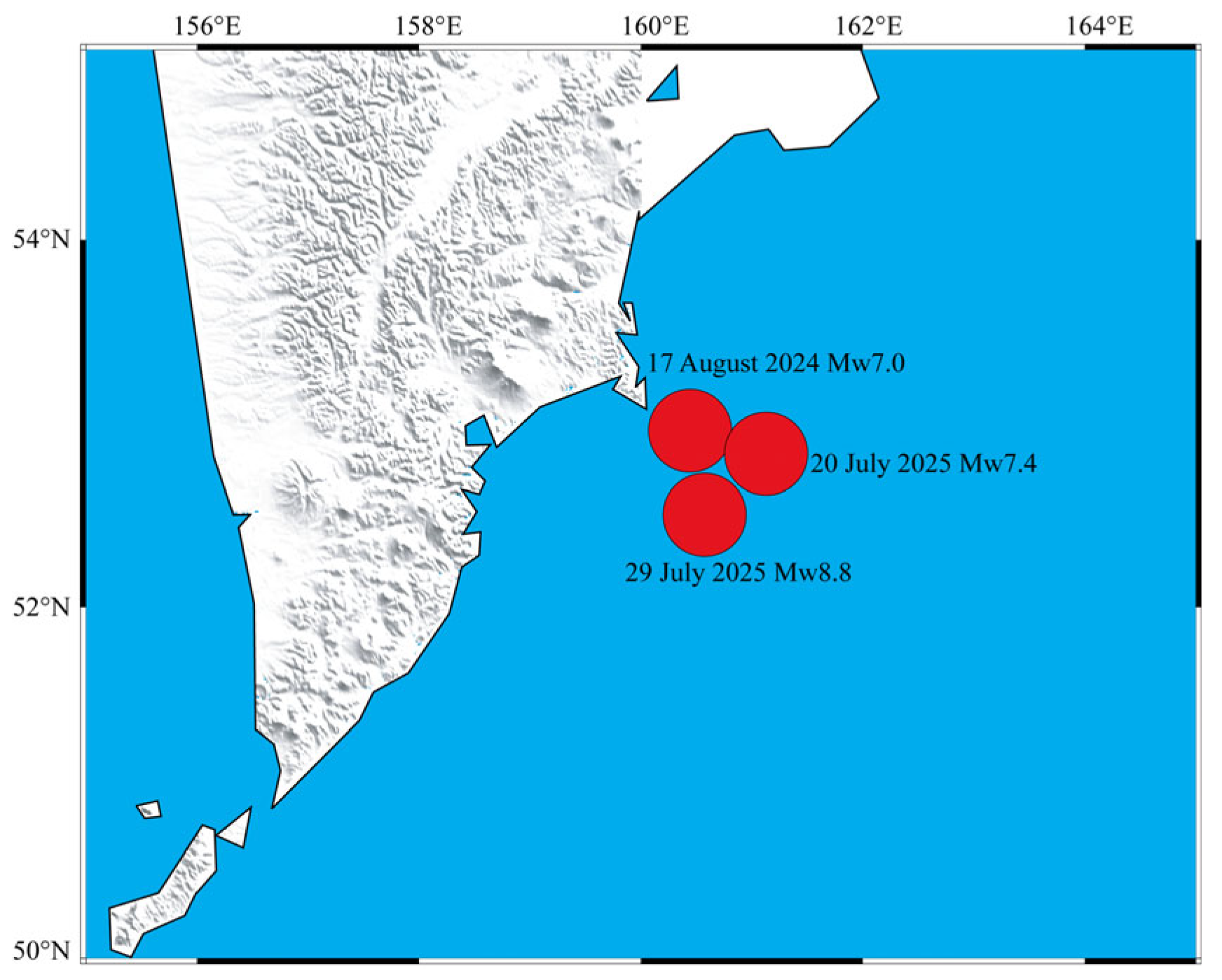
The Kamchatka Peninsula, located in the Russian Far East, is one of the most seismically active regions in the world and sits atop a complex tectonic boundary where the Pacific Plate subducts beneath the Eurasian Plate. This subduction zone is responsible for the intense seismic and volcanic activity in the region. The peninsula features a volcanic arc, including some active volcanoes, which are closely linked to the ongoing tectonic movements and subduction-related stress release. In August 2024, the Mw 7.0 earthquake occurred in this region (Figure 1). Ten days before the 2025 Mw 8.8 mainshock, the Mw 7.4 foreshock occurred on 20 July 2025. Previous analyses suggest that the 20 July 2025 Mw 7.4 event generated an unusually large number of aftershocks, resembling the foreshock behavior observed two days prior to the 2011 Mw 9.0 Tohoku earthquake of Japan [52]. The foreshock-aftershock sequence suggests that the source region was progressively moving toward a rupture unstable state, facilitating the occurrence of the Mw 8.8 mainshock. Notably, the seismic activity in the Kamchatka region follows a quasi-periodic pattern, as the tectonic forces build up along the subduction zone, resulting in cycles of high-intensity earthquakes followed by quiescence. This pattern is a critical aspect of the stress evolution that leads to the mainshock, providing important context for understanding the role of tidal forces in triggering seismic events in this area. The occurrence of large earthquakes in this region is strongly associated with the ongoing tectonic stress accumulation and release as the Pacific plate continues its subduction beneath the Eurasian plate.

2.2. Datasets

Temperature data used in this study were derived from National Centers for Environmental Prediction (NCEP) [53]. This dataset assimilates surface observations, radiosondes, ship, aircraft, and satellite data, ensuring good spatiotemporal continuity. The spatial resolution of the dataset is 1.0° × 1.0°, and the temporal resolution is 6 h. The vertical direction of the data includes 26 standard pressure levels from 1000 hPa to 10 hPa, as well as the surface layer. In this study, the period from 7 July 2025 to 17 August 2025 was selected, with the region defined as 155°E–165°E, 47°N–57°N. To enhance the systematic nature of the analysis, this study integrated multi-source data, including atmospheric temperature, near surface meteorological conditions, volcanic gas emissions, and surface deformation, to assess the observed air temperature excesses and their regional background. The spatiotemporal resolution of these data and their corresponding analytical purposes are shown in Table 1. Among these, NCEP air temperature data served as the core data source for this study, used to describe the vertical evolution of temperature excess signals. The remaining data were mainly used to evaluate possible external disturbances and examine the correspondence of near-surface energy-release indicators. The meteorological assessment in this study was based primarily on regionally averaged sea-level pressure (SLP) and publicly available weather records. However, the meteorological constraint should be regarded as preliminary rather than a complete exclusion of all possible meteorological influences.
It should be noted that the datasets used in this study have different spatial and temporal resolutions, and therefore, they are not interpreted through pixel-by-pixel correspondence. The NCEP air temperature and sea-level pressure fields have a spatial resolution of 1.0° × 1.0° and mainly represent regional-scale atmospheric conditions. In contrast, the Sentinel-5P SO2 product provides finer-scale atmospheric column information, whereas the Sentinel-1A SAR data describe local-scale cumulative line-of-sight deformation between two satellite acquisitions. Considering these scale differences, the multi-source comparison in this study was conducted mainly at a regional scale, focusing on the temporal occurrence, spatial proximity, and overall distribution patterns of the observed signals.

2.3. Tidal Forces Calculation

Tidal forces arise from the combined gravitational attraction of the Moon and the Sun and the centrifugal effect associated with the Earth-Moon barycentric system, and they constitute the fundamental driving force of tides. If a fault zone is already close to failure, the superposition of this periodic, low-amplitude stress-strain perturbation may contribute to earthquake triggering. Statistical and mechanistic studies have suggested that, in some tectonic settings, tidal force is related to earthquake timing, focal depth, and fault orientation [54]. Tidal force varies continuously and exhibits clear periodicity, often characterized by alternating strengthening and weakening phases. Early studies reported associations between changes in the Earth-Moon configuration and moonquake occurrence [55]. Subsequent work further examined tidal–seismic correlations [56,57], and some studies have suggested that larger earthquakes may be more sensitive to tidal perturbations than smaller ones [58,59]. This study introduced tidal force variations not with the intent of considering tidal effects as a direct determinant of earthquake occurrence, but rather as an external background reference with clear periodicity and calculability, used to define the research period and assist in the selection of background days for air temperature excess extraction. Through this method, the potential influence of non-tectonic background interference on pre-earthquake temperature changes could be assessed more cautiously. Using the classical luni-solar tidal-force approach [60], the tidal force variations around the 29 July 2025 Mw 8.8 Kamchatka earthquake was calculated (Figure 2).
For any point P on the Earth’s interior, the tidal force generated is denoted as W i ( P ) :
W i ( P ) = k M r m n = 2 ( r r m ) n P n ( cos Z m )
where k is the gravitational constant; M is the mass of the sun/moon; r m   is the distance from the Earth’s center to the observation point P ; P n ( cos Z m ) is the Legendre polynomial of cos Z m ; Z m is the zenith distance between the point and the celestial body.

2.4. Air Temperature Excess Extraction

To extract potential air temperature excesses related to seismic processes, this study used the background difference method. This method does not simply compare temperature differences between two days; instead, it aims to highlight relative change signals that may be associated with the earthquake process, while minimizing the influences of topography and regional seasonal background effects. The selection of the background day follows two principles: (1) the maximum or minimum of a tidal force cycle is used as the background day; (2) to avoid the background field being influenced by the pre-earthquake process, the background day must be sufficiently separated from the earthquake date. Since this earthquake occurred near the wave peak, the minimum value of the cycle was selected. It should be emphasized that this procedure is not equivalent to an RST-type statistical anomaly detection method. The purpose of the tidal-force-based background day selection is to provide a physically constrained reference for comparing short-term vertical air temperature changes during different tidal force cycles. Because a multi-year climatological reference field was not constructed in this study, the extracted temperature changes should be regarded as air temperature excesses rather than statistically standardized thermal anomalies. In this study, ΔT was calculated as the difference between the air-temperature field on each target date and the corresponding selected background-day temperature field within the same tidal-force cycle. The selected background days, namely 7 July, 20 July, and 5 August, were used as reference fields for their respective comparison periods. In addition, possible meteorological influences were examined at a preliminary level. Specifically, the regional mean sea-level pressure and publicly available weather descriptions were considered to assess whether the observed warming episode coincided with an obvious independent synoptic scale weather system. This method helps reduce background contributions related to topography, land cover differences, and broad meteorological conditions, thereby emphasizing signals that may be associated with the earthquake process. However, this procedure cannot fully eliminate possible meteorological effects. The vertical structure was used as an additional diagnostic feature because near-surface-dominant warming with progressive weakening at higher levels may help distinguish possible near-surface thermal disturbances from ordinary synoptic-scale atmospheric variability. Therefore, the identification of air temperature excesses in this study was based not only on their magnitude, but also on their vertical distribution. If the warming excess is strongest in the near-surface layer and gradually weakens with altitude, it may better fit the expected pattern of tectonically induced thermal perturbations, which are hypothesized to originate from subsurface processes and progressively decay with height. Conversely, if the warming was more pronounced at higher levels and weaker at the near-surface, it is more likely to reflect ordinary weather processes or other non-tectonic factors.
Δ T i ( x , y ) = T i ( x , y ) T b ( x , y )
In Equation (2), Δ T i ( x , y ) represents the increase in air temperature; T i ( x , y ) is the air temperature at different grid points; T b ( x , y ) represents the air temperature background values at different stages; x is the latitude; y is the longitude; i represents different grid points.

2.5. Auxiliary Analyses

To reduce the ambiguity associated with interpreting air temperature excesses from a single parameter, several auxiliary observations were incorporated for cross-validation. SLP, together with publicly available weather records including humidity, wind speed, wind direction, and barometric pressure, was used as a preliminary meteorological constraint to examine whether the study area was affected by an independent strong weather system during the main warming period. The daily weather records were summarized in Table S1. Sentinel-5P SO2 data were used to examine possible variations in volcanic gas emissions during the study period. Because the Kamchatka region is characterized by active volcanism, SO2 variations were interpreted as auxiliary information on regional volcanic-tectonic activity rather than as direct evidence of earthquake preparation. Sentinel-1A InSAR data were used to characterize the deformation background associated with the strong earthquake. These auxiliary datasets were not used to define the air temperature excesses directly, but they provide important constraints for interpreting their possible origin. Because the SAR pair brackets the Mw 8.8 mainshock, the InSAR result was interpreted as cumulative coseismic LOS deformation associated with the mainshock, rather than as preseismic deformation.

3. Results

3.1. Vertical Evolution of Air Temperature Excesses

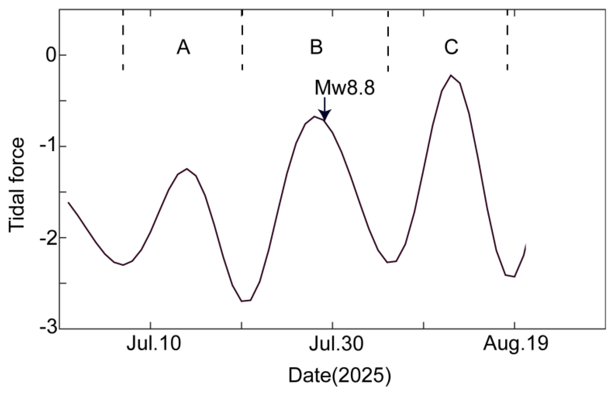
Astronomical tidal forcing relevant to earthquake triggering primarily reflects the gravitational contributions of the Sun and Moon. Following earlier work, the local minimum in each cycle was as the starting point, because the initial phase of a cycle often corresponds to a transition from the previous one. From 7 July 2025, tidal force experienced three consecutive cycles characterized by “trough-peak-trough” behavior, denoted as A, B, and C: cycle A spans 8–19 July, cycle B spans 21 July–4 August, and cycle C spans 6–17 August. Notably, the Mw 8.8 earthquake (arrow in Figure 2) did not occur during cycle A; instead, it occurred near the peak of cycle B. This suggests that the additional stress imposed by tidal force may promote fault slip progressively, while abrupt tidal-stress increases do not necessarily trigger rupture immediately. Rather, rupture occurs when the accumulated tectonic stress reaches a critical threshold [61]. Overall, tidal force may serve as a relevant external factor and provides a useful background reference for temperature analysis. Accordingly, the background days for cycles A, B, and C were selected as 7 July, 20 July, and 5 August, respectively.
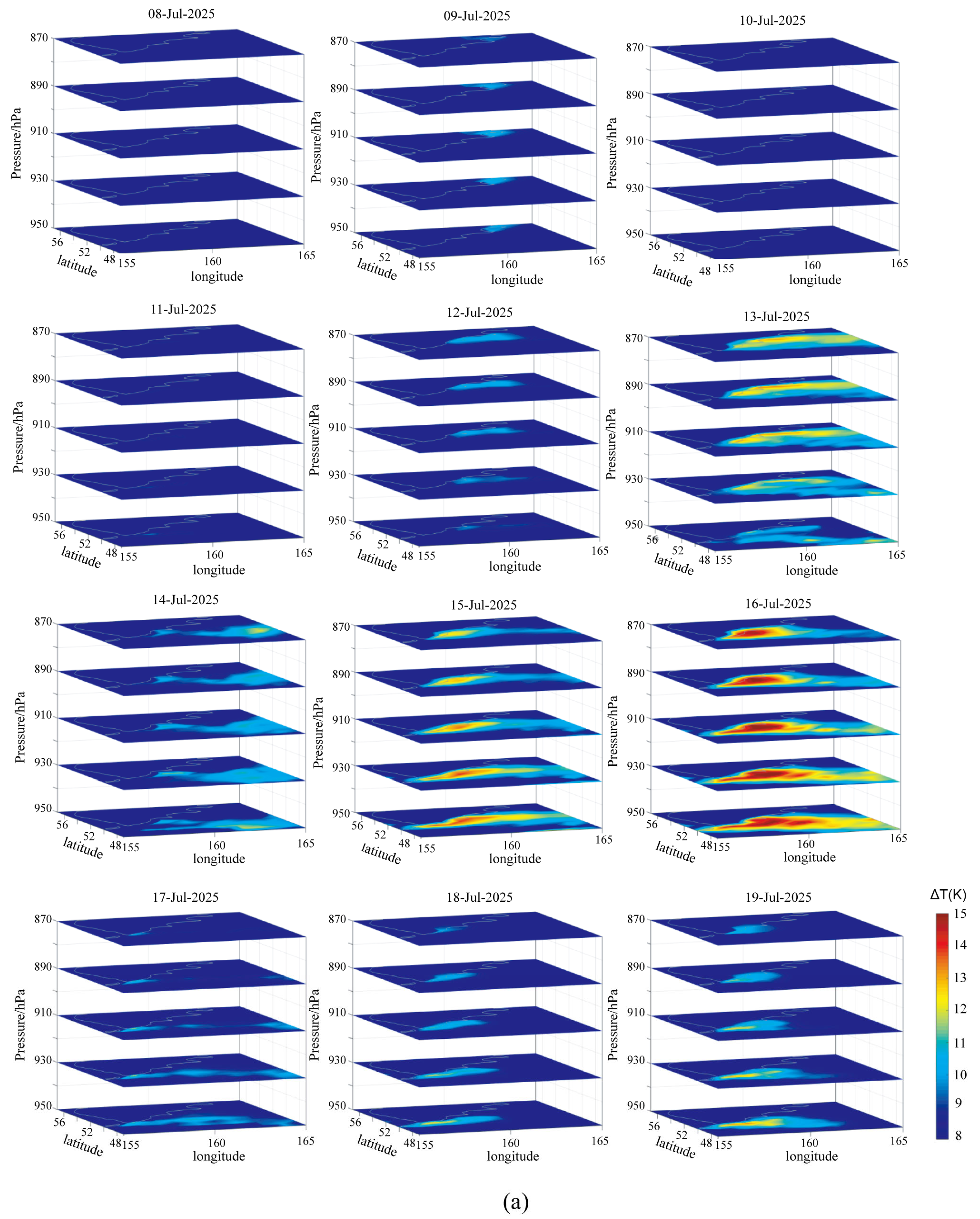
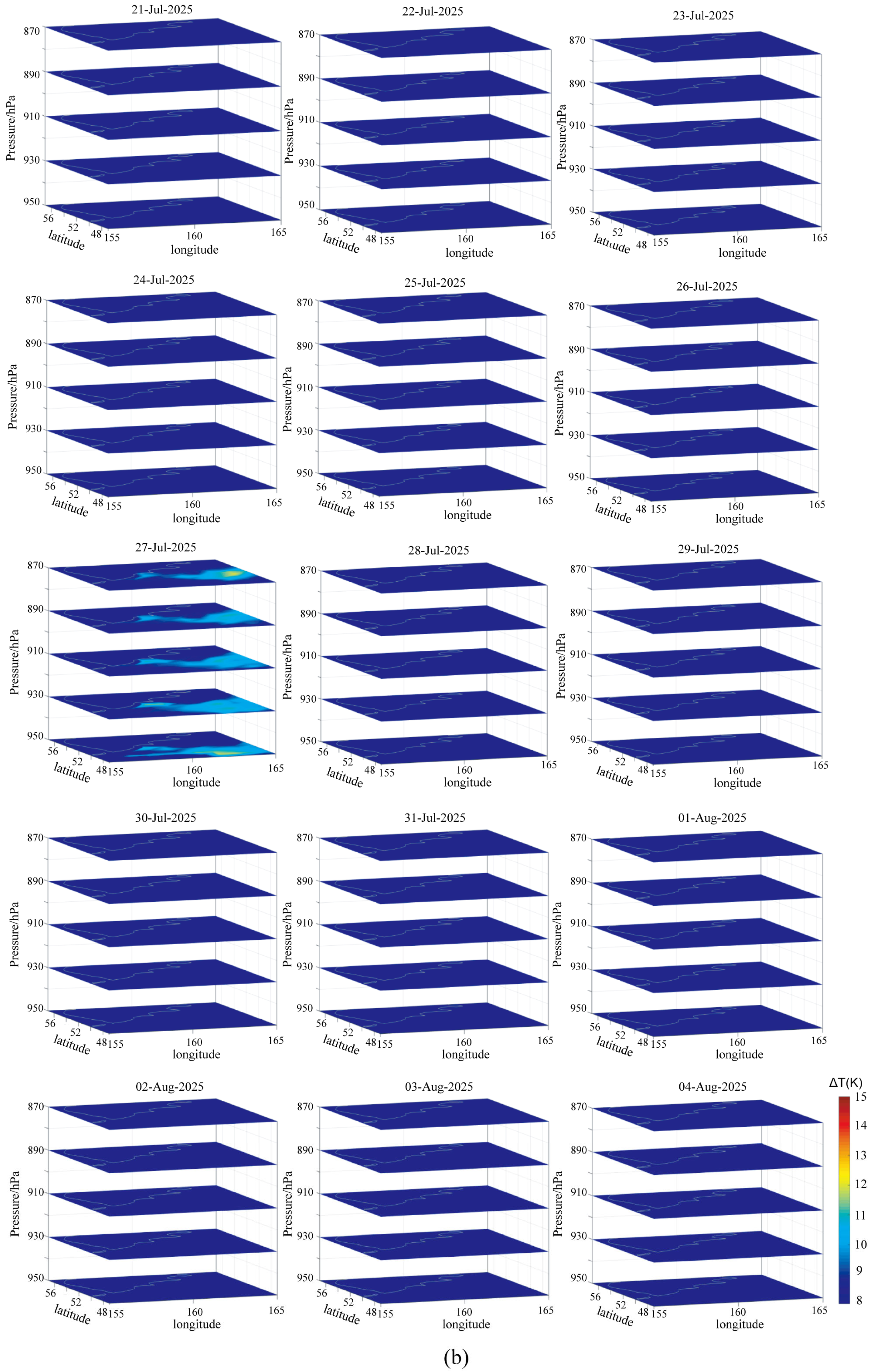
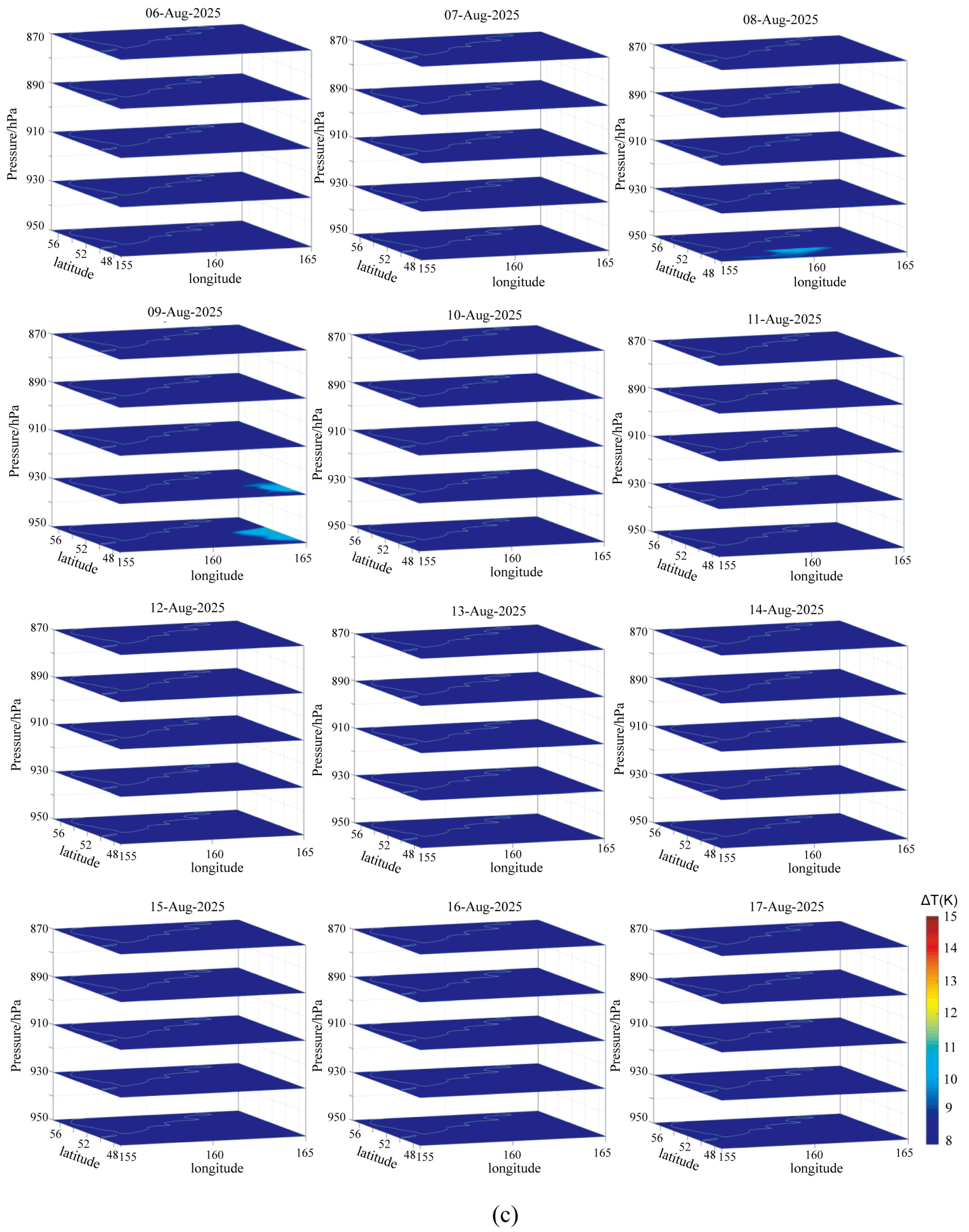
Figure 3 shows air temperature evolution from 950 hPa (near-surface) to 870 hPa (higher level) across the three cycles. During cycle A, warming excesses appeared near the epicentral area on 12–13 July, but the enhancement was stronger aloft than near the surface. This vertical pattern is less consistent with a tectonically driven thermal signal and may instead reflect a non-tectonic or meteorological signal. Beginning on 15 July, a warming excess emerged with larger magnitude and intensity near the surface and progressively weaker warming at higher levels, a pattern that was consistent with the expected signature of tectonically induced thermal perturbations. The warming excess strengthened and peaked on 16 July, weakened on 17–18 July, and showed a weaker warming on 19 July. On 20 July, the Mw 7.4 earthquake occurred near the region of enhanced warming and is considered to be a foreshock to the Mw 8.8 mainshock. Evidence from GPS observations [62], load-unload response ratio studies [63], and rock mechanics experiments [64] indicate that the deformation to rupture process exhibited distinct nonlinear characteristics, making the fluctuation of thermal release during this process physically reasonable. Further analysis showed that, within period B, no marked air temperature excesses occurred prior to the Mw 8.8 mainshock, except for a weak signal on 27 July. This phenomenon suggests that the intensity of air temperature excesses does not have a simple relationship with earthquake magnitude. In this study area, the Mw 7.4 foreshock may have released part of the stress in advance, thereby altering the energy accumulation and release pattern before the mainshock and influencing the temperature excess characteristics. Therefore, this study suggests that air temperature excesses should not be viewed as linear indicators directly corresponding to magnitude, but rather as responses that reflect the characteristics of fault systems at different stages, a mechanism that still requires further verification with additional seismic events.

3.2. SO2 Variations During the Study Period

Since the Kamchatka Peninsula is one of the most volcanically active regions in the world, with numerous active volcanoes, this study further utilized the Sentinel-5P volcanic SO2 data, which is provided through the S5P-PAL platform and is based on Sentinel-5P TROPOMI Level 2 SO2 observations. The spatial resolution of the base product is approximately 3.5 × 5.5 km, and the retrieval is based on TROPOMI spectral observations. The data were filtered using sulfurdioxide_detection_flag > 0 and solar zenith angle (SZA) < 70° to retain more reliable SO2 pixels (https://maps.s5p-pal.com). The SO2 dataset was introduced here as an auxiliary indicator of possible near-surface volatile release. In addition, SO2 concentrations over this region may be influenced by volcanic activity, atmospheric transport, and observation conditions; therefore, SO2 enhancement alone should not be directly attributed to earthquake preparation.
Figure 3. Air temperature variations in the study area during periods A, B, and C. (a) Period A; (b) Period B; (c) Period C. Periods A, B, and C represent different tidal force cycles used for background day selection and target date comparison. The color scale indicates air temperature excesses, ΔT, relative to the selected background days, with units of K. Here, ΔT represents the air temperature field of each target date minus the corresponding selected background day temperature field within the same tidal force cycle.
Remotesensing 18 02306 g003aRemotesensing 18 02306 g003bRemotesensing 18 02306 g003c
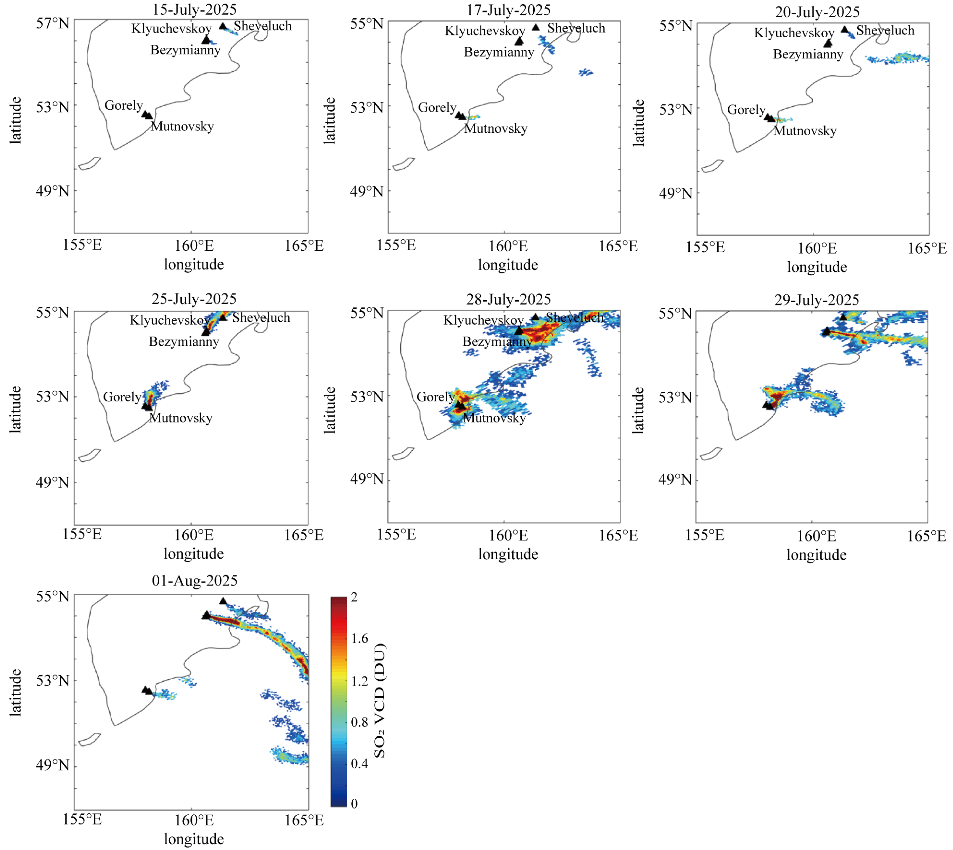
SO2 is a major magmatic gas, and its atmospheric enhancement is commonly associated with volcanic activity. In tectonically active volcanic regions, SO2 variations may also be related to changes in the regional volcanic-tectonic system. Therefore, examining its temporal and spatial evolution may provide auxiliary information for evaluating possible changes in near-surface degassing activity. Observations of SO2 concentrations during the study period revealed a clear enhancement beginning in mid-July 2025, before the 29 July Mw 8.8 Kamchatka mainshock. On 17 July, enhanced SO2 concentrations were observed near the Mutnovsky-Gorely volcanic area in the southeastern part of the Kamchatka Peninsula (Figure 4). During the following days, especially around 28–29 July, the SO2 enhancement became more spatially developed within the study domain. In addition, enhanced SO2 signals were also observed in the northern part of the study area, close to the Klyuchevskoy-Bezymianny-Sheveluch volcanic region. The locations of these representative volcanoes were obtained from the Smithsonian Institution Global Volcanism Program database (https://volcano.si.edu/, accessed on 1 July 2026).
The temporal development of SO2 enhancement before the Mw 8.8 mainshock suggested that the regional volcanic-tectonic system may have experienced enhanced degassing activity during the pre-earthquake period. In the Kamchatka subduction zone, where strong seismicity and active volcanism coexist, variations in volcanic SO2 emissions may provide useful auxiliary information for evaluating changes in the regional volcanic-tectonic background. The occurrence of SO2 enhancement in both the southeastern and northern volcanic regions also indicates that the SO2 signal was not limited to a single volcanic center, but reflected a broader regional volcanic-atmospheric process. Therefore, the SO2 observations were interpreted here as auxiliary evidence for possible changes in regional volcanic-tectonic activity before the Mw 8.8 earthquake. Its relationship with the Mw 8.8 mainshock should be evaluated together with the regional tectonic setting, and other geophysical observations.

3.3. Coseismic Deformation from InSAR

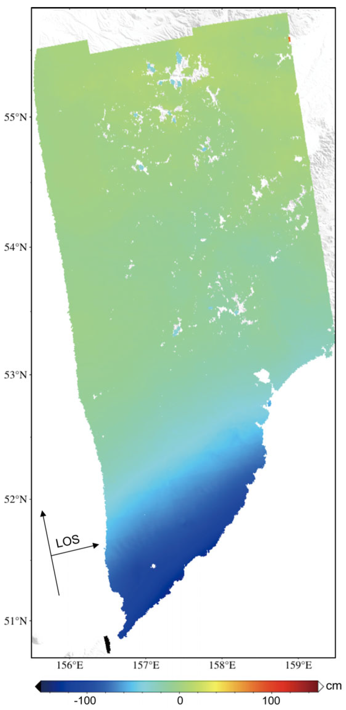
The Mw 8.8 earthquake triggered significant coseismic surface deformation. To characterize the coseismic deformation field, Sentinel-1A ascending-track SAR images acquired on 23 July 2025 and 4 August 2025 were selected as the primary and secondary images, respectively (Figure 5). The temporal baseline of the interferometric pair was 12 days, and the perpendicular baseline was approximately −173 m. Here, the temporal baseline refers to the time interval between the two SAR acquisitions, whereas the perpendicular baseline represents the spatial separation between the two satellite orbits in the direction perpendicular to the radar line of sight. Because the interferometric pair brackets the 29 July 2025 Mw 8.8 mainshock, the resulting deformation field mainly represents cumulative coseismic LOS deformation associated with the mainshock. The 20 July 2025 Mw 7.4 foreshock occurred before the first SAR acquisition; therefore, its immediate coseismic deformation cannot be independently resolved from this interferometric pair. The maximum negative LOS displacement reached approximately −150 cm under the adopted InSAR sign convention. It should be noted that the LOS displacement magnitude was not decomposed into vertical and horizontal components. The D-InSAR method was used to calculate the coseismic deformation. Precise orbit correction was performed using precise orbit ephemeris data, and orbit errors were removed. The SRTM DEM data with 30 m resolution were used to remove the topographic phase, and a distance-to-azimuth view ratio of 20:4 was applied. The Goldstein filtering method was employed to reduce phase noise and enhance coherence. The minimum-cost flow method was used for phase unwrapping, with a coherence threshold of 0.3, and regions below this threshold were excluded from unwrapping to reduce the impact of decorrelation errors. The GACOS model was applied to mitigate atmospheric delay errors. Finally, geographic encoding was performed to obtain the line-of-sight (LOS) deformation.

4. Discussion

The differences in spatial and temporal resolutions among the datasets introduce uncertainties into the interpretation of multi-source signals. The NCEP grid may smooth localized thermal perturbations, whereas the SO2 and InSAR observations may reveal more localized patterns whose centers do not necessarily coincide with the NCEP grid cells. In addition, the InSAR result represents cumulative line-of-sight deformation between two SAR acquisitions, while the air temperature and sea-level pressure fields describe atmospheric conditions at much shorter temporal intervals. Therefore, the observed spatial proximity among air temperature variations, SO2 enhancement, and surface deformation should be interpreted as regional scale consistency rather than direct evidence of point-by-point correspondence. This limitation means that the multi-source evidence supports the presence of possible regional signals, but it cannot by itself prove a unique tectonic origin for the observed air temperature variations. Future work should further evaluate these effects using higher-resolution meteorological data and more complete InSAR data. In particular, the InSAR-derived LOS deformation should be decomposed into vertical and horizontal components, and additional InSAR acquisitions obtained only before the mainshock should be incorporated to examine whether any preseismic crustal deformation existed.
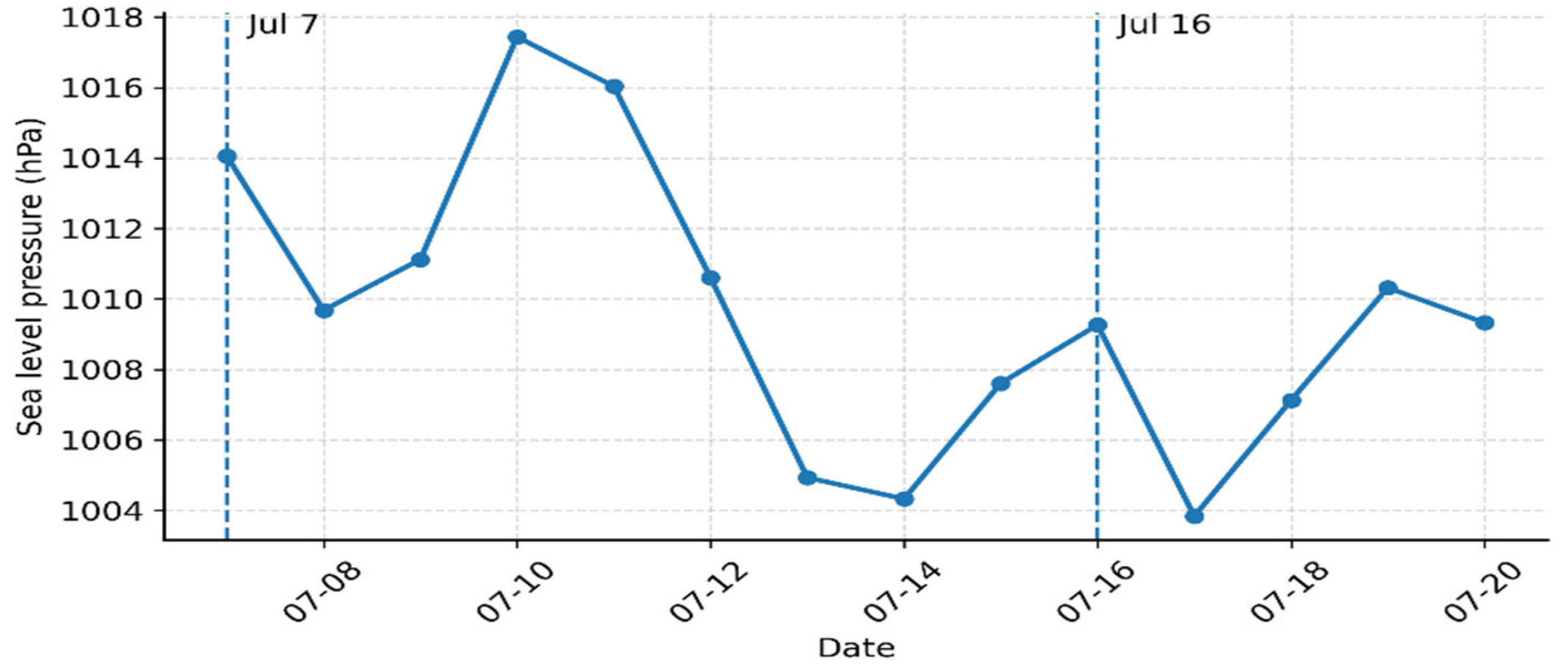
To further assess the meteorological background of the air temperature excesses, this study combined the vertical structure characteristics of near-surface air temperature excesses with concurrent sea-level pressure changes and publicly available weather records. The results showed that from 7 July to 20 July 2025, the regional averaged sea-level pressure over the study area exhibited continuous fluctuations (Figure 6), without showing any abrupt pressure changes corresponding to the period of marked air temperature excesses from 13 to 16 July. This suggests that the study period was less likely to have been directly controlled by an independent strong weather system. Therefore, changes in the near-surface meteorological background alone may not fully explain the nature of the air temperature excesses during this period. Considering the coastal setting of the study area, sea-land thermal interactions may also affect near-surface air temperature; however, the available SLP and public weather records did not provide clear evidence that the observed warming excess was primarily caused by such interactions. Ordinary weather processes alone appear insufficient to fully explain the near-surface-dominant warming excess that appeared after 14 July. Moreover, during the study period, the air temperature in the study area and surrounding regions exhibited typical summer maritime climate characteristics. Publicly available weather records summarized in Table S1 indicate mostly sunny or cloudy conditions, moderate winds, and no reported extreme weather events during the main warming period (https://www.timeanddate.com). However, this structural feature alone is not sufficient to fully exclude all meteorological influences, and further validation using quantitative humidity, precipitation, cloud-cover, and wind-field analyses is still required. More importantly, the warming signal identified in this study was not judged solely by its magnitude, but also by its vertical distribution. The warming episode after 14 July was characterized by a near-surface maximum and a progressive weakening with altitude, which differs from the pattern expected for ordinary synoptic atmospheric forcing. In this sense, the vertical attenuation feature may provide an additional constraint for distinguishing tectonically related warming from meteorological variability.
The pre-earthquake air temperature excesses and enhanced volcanic SO2 emissions may indicate possible changes in the regional volcanic–tectonic system before the Mw 8.8 mainshock. The correspondence between the ΔT and SO2 distributions was mainly reflected in their broad temporal overlap during mid-to-late July and their occurrence within the volcanically and tectonically active Kamchatka region. In this sense, the SO2 enhancement may provide auxiliary information on possible changes in regional degassing activity during the pre-earthquake period. However, the ΔT and SO2 distributions did not show strict point-by-point spatial correspondence. The air temperature excesses were derived from NCEP data with a relatively coarse spatial resolution and mainly represent regional scale atmospheric thermal variations, whereas the Sentinel-5P SO2 observations describe finer-scale atmospheric column concentrations that can be strongly affected by volcanic emission sources, plume dispersion, and observation conditions. Therefore, the relationship between ΔT and SO2 should be interpreted as regional-scale consistency in a volcanically and tectonically active setting.
The InSAR result should be interpreted separately because it represents cumulative coseismic LOS deformation derived from SAR images acquired before and after the mainshock. Therefore, the InSAR deformation field was not used here as evidence of preseismic surface deformation or as a direct measurement of tectonic stress accumulation. Overall, the spatial proximity among the air temperature excesses, SO2 enhancement, and coseismic LOS deformation provided only regional-scale geophysical context for the event, and further multi-source observations are needed to clarify their physical relationships.

5. Conclusions

This study found the presence of marked air temperature excesses preceding the Mw 8.8 earthquake in Kamchatka, Russia. The additional stress exerted by tidal force on critically stressed fault zones may act as a periodic external stress perturbation that can modulate rupture timing when a fault is already close to failure. By analyzing the stratified evolution of air temperature in relation to tidal variations across different periods, a marked enhancement in air temperature was detected near the earthquake epicenter prior to the event. The observed pattern may be consistent with the characteristics commonly associated with tectonically related air temperature excesses: the amplitude and intensity of warming are greatest near the surface and gradually decrease with altitude. This vertical distribution may be related to the fact that thermal radiation associated with tectonic activity primarily originates from within fault zones, resulting in a progressive weakening of the warming signal with height until it dissipates. Compared with approaches based only on surface or bulk thermal changes, the analysis of multi-level atmospheric temperature fields provides additional information on the vertical organization of the warming signal, which is useful for distinguishing possible tectonic signals from non-tectonic disturbances. Based on this characteristic profile, the likelihood that the warming signal was caused solely by ordinary meteorological influences may be reduced to some extent, especially when warming is more pronounced near the surface than at higher altitudes. This distinction may improve the reliability of identifying earthquake-related thermal excesses. The joint consideration of tidal background, atmospheric vertical structure, and auxiliary geophysical observations therefore provides a more integrated framework for evaluating possible pre-earthquake thermal excesses.
In summary, the observed air temperature excesses and enhanced volcanic SO2 emissions before the Mw 8.8 Kamchatka earthquake may provide auxiliary evidence for possible changes in the regional volcanic-tectonic system. However, the SO2 enhancement should be interpreted with caution because it may include contributions from regional volcanic activity, atmospheric transport, and observation conditions, in addition to possible tectonic stress evolution. At the same time, the present study was based on a single earthquake case, and the proposed interpretation still requires further validation using additional earthquakes, volcanic monitoring data, and higher resolution atmospheric datasets, and more complete pre-mainshock geodetic observations. Overall, this study highlighted the potential value of vertical air temperature structure, especially the near-surface-dominant and upward-decaying pattern, as an observational feature that may help improve the identification of tectonically related thermal excesses in future earthquake-related studies.

Supplementary Materials

The following supporting information can be downloaded at: https://www.mdpi.com/article/10.3390/rs18142306/s1, Table S1: Publicly available daily weather records for Petropavlovsk-Kamchatsky from 7 July to 4 August 2025.

Author Contributions

Conceptualization, X.L. and W.M.; methodology, X.L. and J.Z.; validation, W.Y.; writing—original draft preparation, X.L.; writing—review and editing, X.Z.; project administration, X.L.; funding acquisition, X.L. and W.M. All authors have read and agreed to the published version of the manuscript.

Funding

This research was funded by the Xinghuo Science and Technology Program of China Earthquake Administration, grant number XH263705C; the Major Project on High-Resolution Earth Observation, grant number 31-Y30B09-9001-13/15; and the National Natural Science Foundation of China, grant number 41704062.

Data Availability Statement

The data presented in this study are available on request from the corresponding author.

Acknowledgments

The authors gratefully acknowledge the assistance of Xingzhou Wang, Lingyuan Meng, Huaizhong Yu, Anfu Niu and Jing Zhao from the China Earthquake Networks Center during the course of this study.

Conflicts of Interest

The authors declare no conflicts of interest.

References

  1. Jing, F.; Shen, X.H.; Kang, C.L.; Xiong, P. Variations of multi-parameter observations in atmosphere related to earthquake. Nat. Hazards Earth Syst. Sci. 2013, 13, 27–33. [Google Scholar] [CrossRef]
  2. Saraf, A.K.; Choudhury, S. Thermal remote sensing technique in the study of pre-earthquake thermal anomalies. J. Ind. Geophys. Union 2005, 9, 197–207. [Google Scholar]
  3. Tronin, A.; Hayakawa, M.; Molchanov, O.A. Thermal IR satellite data application for earthquake research in Japan and China. J. Geodyn. 2002, 33, 519–534. [Google Scholar] [CrossRef]
  4. Wu, L.X.; Qin, K.; Liu, S. GEOSS-based thermal parameters analysis for earthquake anomaly recognition. Proc. IEEE 2012, 100, 2891–2907. [Google Scholar] [CrossRef]
  5. Qin, K.; Wu, L.X.; De Santis, A.; Meng, J.; Ma, W.Y.; Cianchini, G. Quasi-synchronous multi-parameter anomalies associated with the 2010–2011 New Zealand earthquake sequence. Nat. Hazards Earth Syst. Sci. 2012, 12, 1059–1072. [Google Scholar] [CrossRef]
  6. Liu, D.F.; Luo, Z.L.; Peng, K.Y. OLR anomalies before strong earthquakes. Earthquake 1997, 17, 126–132. [Google Scholar]
  7. Kang, C.L.; Zhang, Y.M.; Liu, D.F.; Jing, F. Long-wave radiation signatures of the 8.0 magnitude Wenchuan earthquake. Earthquake 2009, 29, 116–120. [Google Scholar]
  8. Saradjian, M.R.; Akhoondzadeh, M. Thermal anomalies detection before strong earthquakes (M > 6.0) using interquartile, wavelet, and Kalman filter methods. Nat. Hazards Earth Syst. Sci. 2011, 11, 1139–1148. [Google Scholar] [CrossRef]
  9. Ouzounov, D.; Bryant, N.; Logan, T.; Pulinets, S.; Taylor, P. Satellite thermal IR phenomena associated with some of the major earthquakes in 1999–2003. Phys. Chem. Earth 2006, 31, 154–163. [Google Scholar] [CrossRef]
  10. Pulinets, S.; Ouzounov, D. Lithosphere-Atmosphere-Ionosphere Coupling (LAIC) model—A unified concept for earthquake precursors validation. J. Asian Earth Sci. 2011, 41, 371–382. [Google Scholar] [CrossRef]
  11. Pulinets, S. Low-latitude atmosphere-ionosphere effects initiated by strong earthquakes preparation process. Int. J. Geophys. 2012, 2012, 131842. [Google Scholar] [CrossRef]
  12. Draz, M.U.; Shah, M.; Jamjareegulgarn, P.; Shahzad, R.; Hasan, A.M.; Ghamry, N.A. Deep machine learning based possible atmospheric and ionospheric precursors of the 2021 Mw 7.1 Japan earthquake. Remote Sens. 2023, 15, 1904. [Google Scholar] [CrossRef]
  13. Shah, M.; Shahzad, R.; Jamjareegulgarn, P.; Ghaffar, B.; Oliveira-Junior, J.F.; Hassan, A.M.; Ghamry, N.A. Machine-learning-based lithosphere-atmosphere-ionosphere coupling associated with Mw > 6 earthquakes in America. Atmosphere 2023, 14, 1236. [Google Scholar] [CrossRef]
  14. Liu, W.; Liu, S.; Wei, L.; Han, X.; Zhu, A. Experimental study on the thermal response of rocks to stress change and its significance. Geophys. J. Int. 2024, 238, 557–572. [Google Scholar] [CrossRef]
  15. Freund, F.T.; Takeuchi, A.; Lau, B.W.; Al-Manaseer, A.; Fu, C.C.; Bryant, N.A.; Ouzounov, D. Stimulated infrared emission from rocks: Assessing a stress indicator. Earth 2007, 2, 7–16. [Google Scholar] [CrossRef]
  16. Zhang, Y.S.; Guo, X.; Zhong, M.J.; Shen, W.R.; Li, W.; He, B. Thermal infrared brightness temperature changes before the Wenchuan Earthquake. Sci. Bull. 2010, 55, 904–910. [Google Scholar] [CrossRef]
  17. Xie, T.; Ma, W. Possible thermal brightness temperature anomalies associated with the Lushan (China) MS7.0 earthquake on 20 April 2013. Earthq. Sci. 2014, 27, 49–58. [Google Scholar] [CrossRef]
  18. Lu, X.; Meng, Q.Y.; Gu, X.F.; Zhang, X.D.; Xie, T.; Geng, F. Thermal infrared anomalies associated with multi-year earthquakes in the Tibet region based on China’s FY-2E satellite data. Adv. Space Res. 2016, 58, 989–1001. [Google Scholar] [CrossRef]
  19. Jing, F.; Singh, R.P.; Cui, Y.; Sun, K. Microwave brightness temperature characteristics of three strong earthquakes in Sichuan Province, China. IEEE J. Sel. Top. Appl. Earth Obs. Remote Sens. 2020, 13, 513–522. [Google Scholar] [CrossRef]
  20. Jing, F.; Jiang, M.; Singh, R.P. Detection of seismic microwave radiation anomalies in snow-covered mountainous terrain: Insights from two recent earthquakes in the Pamir–Tien Shan region. IEEE J. Sel. Top. Appl. Earth Obs. Remote Sens. 2024, 17, 18156–18166. [Google Scholar] [CrossRef]
  21. Liu, S.; Cui, Y.; Wei, L.; Liu, W.; Ji, M. Pre-earthquake MBT anomalies in the Central and Eastern Qinghai-Tibet Plateau and their association to earthquakes. Remote Sens. Environ. 2023, 298, 113815. [Google Scholar] [CrossRef]
  22. Maki, K.; Takano, T.; Soma, E.; Ishii, K.; Yoshida, S.; Nakatani, M. An experimental study of microwave emission from compression failure of rocks. J. Seismol. Soc. Jpn. 2006, 58, 375–384. [Google Scholar] [CrossRef]
  23. Liu, S.; Xu, Z.; Wei, J.; Huang, J.; Wu, L. Experimental study on microwave radiation from deforming and fracturing rock under loading outdoor. IEEE Trans. Geosci. Remote Sens. 2016, 54, 5578–5587. [Google Scholar] [CrossRef]
  24. Ouzounov, D.; Liu, D.; Kang, C.L.; Cervone, G.; Kafatos, M.; Taylor, P. Outgoing long wave radiation variability from IR satellite data prior to major earthquakes. Tectonophysics 2007, 431, 211–220. [Google Scholar] [CrossRef]
  25. Su, B.; Li, H.; Ma, W.Y.; Zhao, J.; Yao, Q.; Cui, J.; Chong, Y.; Kun, C.L. The outgoing longwave radiation analysis of medium and strong earthquakes. IEEE J. Sel. Top. Appl. Earth Obs. Remote Sens. 2021, 14, 6962–6973. [Google Scholar] [CrossRef]
  26. Guo, X.; Zhang, Y.S.; Zhong, M.J.; Shen, W.R.; Wei, C.X. Variation characteristics of OLR for the Wenchuan earthquake. Chin. J. Geophys. 2010, 53, 2688–2695. [Google Scholar] [CrossRef]
  27. Xiong, P.; Shen, X.H.; Bi, Y.X.; Kang, C.L.; Chen, L.Z.; Jing, F.; Chen, Y. Study of outgoing longwave radiation anomalies associated with Haiti earthquake. Nat. Hazards Earth Syst. Sci. 2010, 10, 2169–2178. [Google Scholar] [CrossRef]
  28. Chakraborty, S.; Sasmal, S.; Chakrabarti, S.K.; Bhattacharya, A. Observational signatures of unusual outgoing longwave radiation (OLR) and atmospheric gravity waves (AGW) as precursory effects of May 2015 Nepal earthquakes. J. Geodyn. 2018, 113, 43–51. [Google Scholar] [CrossRef]
  29. Zhang, Z. Shallow ground temperature and its relation to strong earthquakes. Earthquake 1994, 14, 73–80. [Google Scholar]
  30. Bellaoui, M.; Hassini, A.; Kada, B. Pre-seismic anomalies in remotely sensed land surface temperature measurements: The case study of 2003 Boumerdes earthquake. Adv. Space Res. 2017, 59, 2645–2657. [Google Scholar] [CrossRef]
  31. Chen, S.; Liu, P.; Liu, L.; Ma, J. Changes in the ground temperature in Kangding prior to the Lushan earthquake. Earthq. Geol. 2013, 35, 634–640. [Google Scholar]
  32. Min, W.B.; Xu, X.L. Preliminary analysis of surface temperature variation characteristics before and after the 5.12 Wenchuan earthquake. Plateau Mt. Meteorol. Res. 2008, 28, 42–46. [Google Scholar]
  33. Jiao, Z.H.; Shan, X.J. Consecutive statistical evaluation framework for earthquake forecasting: Evaluating satellite surface temperature anomaly detection methods. J. Asian Earth Sci. X 2022, 7, 100096. [Google Scholar] [CrossRef]
  34. Pulinets, S.A.; Dunajecka, M.A. Specific variations of air temperature and relative humidity around the time of Michoacan earthquake M8.1 19 September 1985 as a possible indicator of interaction between tectonic plates. Tectonophysics 2007, 431, 221–230. [Google Scholar] [CrossRef]
  35. Mahmood, I. Anomalous variations of air temperature prior to earthquakes. Geocarto Int. 2019, 36, 1396–1408. [Google Scholar] [CrossRef]
  36. Mahmood, I.; Iqbal, M.F.; Shahzad, M.I.; Qaiser, S. Investigation of atmospheric anomalies associated with Kashmir and Awaran earthquakes. J. Atmos. Sol.-Terr. Phys. 2017, 154, 75–85. [Google Scholar] [CrossRef]
  37. Ghosh, S.; Chowdhury, S.; Kundu, S.; Sasmal, S.; Politis, D.Z.; Potirakis, S.M.; Hayakawa, M.; Chakraborty, S.; Chakrabarti, S.K. Unusual surface latent heat flux variations and their critical dynamics revealed before strong earthquakes. Entropy 2022, 24, 23. [Google Scholar]
  38. Dey, S.; Singh, R. Surface latent heat flux as an earthquake precursor. Nat. Hazards Earth Syst. Sci. 2003, 3, 749–755. [Google Scholar] [CrossRef]
  39. Cervone, G.; Kafatos, M.; Napoletani, D.; Singh, R.P. Wavelet maxima curves of surface latent heat flux associated with two recent Greek earthquakes. Nat. Hazards Earth Syst. Sci. 2004, 4, 359–374. [Google Scholar] [CrossRef]
  40. Chen, M.H.; Deng, Z.H.; Yang, Z.Z.; Ma, X.J. Latent heat flux anomalies before the 2004 Indonesian 9.0 earthquake. Sci. Bull. 2006, 51, 118–120. [Google Scholar] [CrossRef]
  41. Chakraborty, S.; Sasmal, S.; Basak, T.; Ghosh, S.; Palit, S.; Chakrabarti, S.K.; Ray, S. Numerical modeling of possible lower ionospheric anomalies associated with Nepal earthquake in May 2015. Adv. Space Res. 2017, 60, 1787–1796. [Google Scholar] [CrossRef]
  42. Harrison, R.G.; Aplin, K.L.; Rycroft, M.J. Atmospheric electricity coupling between earthquake regions and the ionosphere. J. Atmos. Sol.-Terr. Phys. 2010, 72, 376–381. [Google Scholar] [CrossRef]
  43. Song, R.; Hattori, K.; Zhang, X.M.; Sanaka, S. Seismic-ionospheric effects prior to four earthquakes in Indonesia detected by the China seismo-electromagnetic satellite. J. Atmos. Sol.-Terr. Phys. 2020, 205, 105291. [Google Scholar] [CrossRef]
  44. Singh, O.P.; Chauhan, V.; Singh, V.; Singh, B. Anomalous variation in total electron content (TEC) associated with earthquakes in India during September 2006–November 2007. Phys. Chem. Earth 2009, 34, 479–484. [Google Scholar] [CrossRef]
  45. Liu, J.; Huang, J.P.; Zhang, X.M. Ionospheric perturbations in plasma parameters before global strong earthquakes. Adv. Space Res. 2014, 53, 776–787. [Google Scholar] [CrossRef]
  46. Singh, R.P.; Kumar, J.S.; Zlotnicki, J.; Kafatos, M. Satellite detection of carbon monoxide emission prior to the Gujarat earthquake of 26 January 2001. Appl. Geochem. 2010, 25, 580–585. [Google Scholar] [CrossRef]
  47. Dey, S.; Sarkar, S.; Singh, R.P. Anomalous changes in column water vapor after Gujarat earthquake. Adv. Space Res. 2004, 33, 274–278. [Google Scholar] [CrossRef]
  48. Tramutoli, V.; Di Bello, G.; Pergola, N.; Piscitelli, S. Robust Satellite Techniques for Remote Sensing of Seismically Active Areas. Ann. Geophys. 2001, 44, 295–312. [Google Scholar] [CrossRef]
  49. Kilston, S.; Knopoff, L. Lunaresolar periodicities of large earthquakes in southern California. Nature 1983, 304, 21–25. [Google Scholar] [CrossRef]
  50. Wang, W.; Shearer, P.M.; Vidale, J.E.; Xu, X.; Trugman, D.T.; Fialko, Y. Tidal modulation of seismicity at the Coso geothermal field. Earth Planet. Sci. Lett. 2022, 579, 117335. [Google Scholar] [CrossRef]
  51. Xu, X.; Wang, L.; Chen, S. Analysis of Ocean–Lithosphere–Atmosphere–Ionosphere Coupling Related to Two Strong Earthquakes Occurring in June–September 2022 on the Sea Coast of Philippines and Papua New Guinea. Remote Sens. 2023, 15, 4392. [Google Scholar] [CrossRef]
  52. Stein, R.S.; Toda, S.; Lotto, G.; Gonzalez-Huizar, H.; Sevilgen, V. Huge July 2025 Kamchatka Earthquake Followed Unusually Productive Foreshock Sequence. 2025. Available online: https://temblor.net/earthquake-insights/huge-july-2025-kamchatka-earthquake-follows-unusually-productive-foreshock-sequence-16866/ (accessed on 4 July 2026).
  53. Kalnay, E.; Kanamitsu, M.; Kistler, R.; Collins, W.; Deaven, D.; Gandin, L.; Iredell, M.; Saha, S.; White, G.; Woollen, J.; et al. The NCEP/NCAR 40-year reanalysis project. Bull. Am. Meteorol. Soc. 1996, 77, 437–471. [Google Scholar] [CrossRef]
  54. Tanaka, S.; Ohtake, M.; Sato, H. Evidence for tidal triggering of earthquakes as revealed from statistical analysis of global data. J. Geophys. Res. 2002, 107, 2211. [Google Scholar] [CrossRef]
  55. Lammlein, D.R.; Latham, G.V.; Dorman, J.; Nakamura, Y.; Ewing, M. Lunar seismicity, structure and tectonics. Rev. Geophys. 1974, 12, 1–21. [Google Scholar] [CrossRef]
  56. Heaton, T.H. Tidal triggering of earthquakes. Geophys. J. R. Astron. Soc. 1975, 43, 307–326. [Google Scholar] [CrossRef]
  57. Tanaka, S.; Ohtake, M.; Sato, H. Spatio-temporal variation of the tidal triggering effect on earthquake occurrence associated with the 1982 South Tonga earthquake of Mw 7.5. Geophys. Res. Lett. 2002, 29, 1756. [Google Scholar] [CrossRef]
  58. Allen, M.W. The lunar triggering of earthquakes in Southern California. Bull. Seismol. Soc. Am. 1936, 26, 147–157. [Google Scholar] [CrossRef]
  59. Tamrazyan, G.P. Principal regularities in the distribution of major earthquakes relative to solar and lunar tides and other cosmic sources. Icarus 1968, 9, 574–592. [Google Scholar] [CrossRef]
  60. Cartwright, D.E.; Tayler, R.J. New computations of the tide-generating potential. Geophys. J. R. Astron. Soc. 1971, 23, 45–74. [Google Scholar] [CrossRef]
  61. Ma, W.Y.; Wang, H.; Li, F.S.; Ma, W.M. Relation between the celestial tide-generating stress and the temperature variations of the Abruzzo M6.3 earthquake in April 2009. Nat. Hazards Earth Syst. Sci. 2012, 12, 819–827. [Google Scholar] [CrossRef]
  62. Wnęk, A.; Kudas, D. Determination of trends in GPS time series using complementary ensemble empirical mode decomposition. Remote Sens. 2025, 17, 2802. [Google Scholar] [CrossRef]
  63. Jia, D.H.; Yu, H.Z.; Chen, J.H.; Yan, R.; Liu, J.; Zhao, B.B.; Li, Z.P.; Ma, Y.C.; Yuan, Z.Y.; Yang, W.; et al. Exploring strong earthquake nucleation process using the unloading response ratio: A case study of the 2020 Kashi 6.4 earthquake in Xinjiang. Acta Geophys. 2024, 67, 2232–2247. [Google Scholar]
  64. Wu, L.X.; Cui, C.Y.; Geng, N.G.; Wang, J.Z. Remote sensing rock mechanics (RSRM) and associated experimental studies. Int. J. Rock Mech. Min. Sci. 2000, 37, 879–888. [Google Scholar] [CrossRef]
Figure 1. Spatial distribution of earthquakes with Mw ≥ 7.0 in the study area of the Kamchatka Peninsula from January 2024 to August 2025. The red circles represent earthquakes.
Remotesensing 18 02306 g001
Figure 2. Variations in tidal force before and after the Mw 8.8 Kamchatka earthquake from July to August 2025. A represents Period A; B represents Period B; C represents Period C.
Remotesensing 18 02306 g002
Figure 4. Spatial distribution of daily Sentinel-5P/TROPOMI volcanic SO2 vertical column density over southeastern Kamchatka from 15 July to 1 August 2025. The color scale indicates SO2 vertical column density under the 7 km SO2 plume-height assumption, with values ranging from 0 to 2 DU. The data were obtained from the S5P-PAL Copernicus Sentinel-5P Mapping Portal Volcanic SO2 (7 km) daily product, which is based on Sentinel-5P/TROPOMI Level-2 SO2 observations with a nadir ground-pixel resolution of approximately 3.5 × 5.5 km. Black triangles denote the locations of the representative volcanoes.
Remotesensing 18 02306 g004
Figure 5. Cumulative coseismic line-of-sight (LOS) deformation associated with the 2025 Mw 8.8 Kamchatka earthquake, derived from Sentinel-1A ascending-track SAR images acquired on 23 July and 4 August 2025. Negative LOS values indicate motion away from the satellite under the adopted sign convention, whereas positive values indicate motion toward the satellite. The arrow indicates the approximate LOS viewing direction.
Remotesensing 18 02306 g005
Figure 6. Temporal variation of the regionally averaged sea-level pressure (SLP) over the study area from 7 to 20 July 2025. The SLP was averaged over the domain (155°E–165°E, 47°N–57°N). The dashed lines denote the background day (7 July) and the peak warming day (16 July) of the air temperature excess, respectively. These two dates were used to compare near-surface meteorological characteristics between the background and warming periods.
Remotesensing 18 02306 g006
Table 1. Data sources, resolutions, applications and main uncertainties.
Data NameTime
Resolution
Spatial
Resolution
PurposeScale RepresentedMain Uncertainty
NCEP air temperature6 h1.0° × 1.0°Detect vertical air temperature variationsRegional-scale atmospheric backgroundSpatial smoothing; localized signals may be weakened
Sentinel-5P SO21 day3.5 × 5.5 kmMonitor SO2 enhancementMesoscale atmospheric column informationCloud cover, wind transport
Sentinel-1A SARAcquisition-pair interval20 mDetect surface deformationLocal-scale cumulative LOS deformationRepresents cumulative deformation between two acquisitions; cannot be directly compared with daily atmospheric fields
SLP6 h1.0° × 1.0°Examine meteorological backgroundRegional-scale pressure fieldMay not capture local convective or mesoscale weather processes
Disclaimer/Publisher’s Note: The statements, opinions and data contained in all publications are solely those of the individual author(s) and contributor(s) and not of MDPI and/or the editor(s). MDPI and/or the editor(s) disclaim responsibility for any injury to people or property resulting from any ideas, methods, instructions or products referred to in the content.