Article

Cross-Domain Land Surface Temperature Retrieval via Strategic Fine-Tuning-Based Transfer Learning: Application to GF5-02 VIMI Imagery

1
Aerospace Information Research Institute, Chinese Academy of Sciences, Beijing 100101, China
2
Hangzhou International Innovation Institute, Hangzhou 311115, China
3
School of Transportation Science and Engineering, Beihang University, Beijing 100191, China
4
School of Instrumentation Science and Opto-Electronics Engineering, Beihang University, Beijing 100191, China
5
State Key Laboratory of Earth Surface Processes and Disaster Risk Reduction, Advanced Interdisciplinary Institute of Satellite Applications, Faculty of Geographical Science, Beijing Normal University, Beijing 100875, China
*
Author to whom correspondence should be addressed.
Remote Sens. 2025, 17(23), 3803; https://doi.org/10.3390/rs17233803 (registering DOI)
Submission received: 26 September 2025 / Revised: 18 November 2025 / Accepted: 20 November 2025 / Published: 23 November 2025

Highlights

What are the main findings?
  • A three-stage SFTL framework enhances GF5-02/VIMI LST retrieval by combining large simulated datasets with limited in situ measurements and shows that in situ sample size and statistical variability determine the optimal neural network and fine-tuning strategy.
  • The framework achieves strong cross-site generalization (≈2.9–3.4 K RMSE), outperforming both Split-Window and direct-training machine-learning models.
What are the implications of the main findings?
  • The approach enables reliable LST mapping in regions with sparse ground observations, reducing dependence on large labeled in situ datasets.
  • The method offers a scalable route for operational GF5-02/VIMI LST retrieval across heterogeneous surface types and atmospheric conditions.

Abstract

Accurate prediction of land surface temperature (LST) is critical for remote sensing applications, yet remains hindered by in situ data scarcity, limited input variables, and regional variability. To address these limitations, we introduce a three-stage strategic fine-tuning-based transfer learning (SFTL) framework that integrates a large simulated dataset (430 K samples), in situ measurements from the Heihe and Huailai regions in China, and high-resolution imagery from the GF5-02 Visible and Infrared Multispectral Imager (VIMI). The key novelty of this study is the combination of large-scale simulation, an engineered humidity-sensitive feature, and multiple parameter-efficient tuning strategies—full, head, gradual, adapter, and low-rank adaptation (LoRA)—within a unified transfer-learning framework for cross-site LST estimation. In Stage 1, pre-training with 5-fold cross-validation on the simulated dataset produced strong baseline models, including Random Forest (RF), Light Gradient Boosting Machine (LGBM), Deep Neural Network (DNN), Transformer (TrF), and Convolutional Neural Network (CNN). In Stage 2, strategic fine-tuning was conducted under two cross-regional scenarios—Heihe-to-Huailai and Huailai-to-Heihe—and model transfer for tree-based learners. Fine-tuning achieved competitive in-domain performance while materially improving cross-site transfer. When trained on Huailai and tested on Heihe, DNN-gradual attained RMSE 2.89 K (R2 ≈ 0.96); when trained on Heihe and tested on Huailai, TrF-head achieved RMSE 3.34 K (R2 ≈ 0.94). In Stage 3, sensitivity analyses confirmed stability across IQR multipliers of 1.0–1.5, with <1% RMSE variation across models and sites, indicating robustness against outliers. Additionally, application to real GF5-02 VIMI imagery demonstrated that the best SFTL configurations aligned with spatiotemporal in situ observations at both sites, capturing the expected spatial gradients. Overall, the proposed SFTL framework—anchored in cross-validation, strategic fine-tuning, and large-scale simulation—outperforms the widely used Split-Window (SW) algorithm (Huailai: RMSE = 3.64 K; Heihe: RMSE = 4.22 K) as well as direct-training Machine Learning (ML) models, underscoring their limitations in modeling complex regional variability.

1. Introduction

As a pivotal environmental parameter, land surface temperature (LST) is integral to various Earth system processes and plays a significant role in surface–atmosphere interactions, climate research, and ecosystem functionality [1,2,3,4,5,6]. It has been broadly utilized in several domains, for instance, climate change [7,8,9,10,11], soil moisture and evapotranspiration estimations [12,13,14], urban climate monitoring [15,16,17,18], and hydrology [19,20,21]. Recognized as an Essential Climate Variable (ECV) by the Global Climate Observing System (GCOS) and NASA [6,22,23,24], LST is vital for environmental monitoring and research. With respect to this, in situ measurements offer limited point-scale LST observations, which are insufficient for capturing spatial thermal variability [25]. In contrast, satellite remote sensing—particularly Thermal Infrared (TIR) data from sensors like Visible and Infrared Multispectral Imager (VIMI) on the GF5-02 satellite—offers continuous, high-resolution LST mapping with a 40 m full spatial resolution across a 60 km wide swath [1,26,27]. Equipped with four TIR channels, VIMI supports disaster monitoring, water resource management, and ecological studies [28,29,30], although such sensors remain scarce [4].
Since the VIMI sensor’s emergence, various algorithms have been applied for LST retrieval, such as the Split-Window (SW) algorithm [28,29,30,31,32,33], Nonlinear Split-Window (NSW) algorithm [34,35], the hybrid (temperature and emissivity separation (TES)-SW) algorithm [35], and Deep Learning-based (DL) approaches [36]. The Split-Window (SW) algorithm is one of the most widely used methods for LST retrieval, as it minimizes the need for atmospheric data by removing atmospheric effects through a linear or nonlinear combination of brightness temperatures (BTs) from adjacent TIR channels of the VIMI sensor [26,30,37]. To further reduce errors caused by uncertainties in atmospheric correction and land surface emissivity (LSE), the hybrid TES-SW algorithm was developed. This method eliminates the need for external inputs by relying solely on top-of-atmosphere BTs. It combines the SW algorithm to correct atmospheric effects and the TES algorithm to simultaneously retrieve LST and emissivity [37,38]. However, TES tends to introduce significant errors for surfaces with low spectral emissivity contrast [28,39]. Except for the TES-SW algorithm, all the aforementioned methods require external auxiliary data beyond TIR observations to resolve the ill-posed nature of the Radiative Transfer Equation (RTE) in single-channel or multispectral TIR remote sensing [4,5,6]. These dependencies can introduce further inaccuracies due to mismatches in spatial resolution or temporal alignment among data sources [5,40]. Simulated datasets play a crucial role in evaluating the theoretical accuracy of LST retrieval algorithms. However, accuracy derived from simulated data often exceeds that of real-world applications using in situ measurements, due to the complexities of natural observation environments [41].
Unlike physics-based algorithms, learning-based approaches [42] have proven effective for retrieving remote sensing parameters, owing to their strong feature extraction and nonlinear problem-solving capabilities [43,44,45]. These methods can model complex relationships between land surface and atmospheric variables and the at-sensor measured thermal radiance [40,42]. However, DL models require considerable resources, including extensive training time, high-performance hardware, substantial data storage, and expert tuning [43]. To address these limitations, the strategic fine-tuning-based transfer learning (SFTL) framework allows models trained on a source task to be reused for a related target task without retraining from scratch or modifying the original weights [42,46]. SFTL leverages prior knowledge across domains, reducing the dependency on large labeled datasets [43], and directly addresses one of the key challenges in remote sensing: limited well-labeled training data [11,47]. Furthermore, unlike traditional machine learning (ML) models that struggle with distribution mismatches, transfer learning (TL) overcomes this by integrating knowledge from one or more source domains into the target application [48], thereby improving generalization and efficiency.
Despite recent advancements, LST retrieval remains challenged by data scarcity, regional variability, and computational complexity, prompting innovative research. Ye et al. [37] proposed a hybrid algorithm using Gaofen-5 TIR data for simultaneous retrieval of LST and emissivity. Ru et al. [4] extended the TES-SW algorithm with urban geometry correction, though it retains TES’s limitations on surfaces with low spectral emissivity contrast. In the learning-based domain, Ye et al. [40] applied deep learning to improve LST retrieval through enhanced feature extraction, but their model was limited by insufficient labeled training data. Wang et al. [11] applied a transfer-based framework with DNN and U-Net to enhance near-surface air temperature estimates in data-sparse regions, though fine-tuning strategies remained underexplored. Similarly, Xu et al. [8] proposed a TL approach to estimate LST from Landsat TOA data; however, the framework lacks the robustness needed to fully address both data scarcity and regional variability. More recently, Fathi et al. [49] employed knowledge transfer and multi-source data fusion for super-resolution LST, yet their approach still required a large volume of labeled data and extensive data collection.
Building on recent advancements, this study introduces a novel three-stage SFTL framework to tackle persistent challenges in LST retrieval, including data scarcity, regional variability, limited input variables, and computational complexity. Unlike prior approaches that rely on large labeled datasets or single-model strategies, our framework begins with a robust pre-training phase using K-fold cross-validation (KF-CV) on a large simulated dataset to ensure stability and generalizability. This is followed by a strategic fine-tuning phase, in which five advanced adaptation techniques—full, head, gradual, adapter, and low-rank adaptation (LoRA)—are evaluated across neural network (NN) models. Two regional transfer scenarios are examined: (1) pre-training on the simulated dataset → fine-tuning and testing on the Huailai in situ dataset → generalization testing on the Heihe dataset (SiHuHe), and (2) pre-training on the simulated dataset → fine-tuning and testing on the Heihe dataset → generalization testing on the Huailai dataset (SiHeHu). Finally, the validated framework is applied on real GF5-02 VIMI imagery, benchmarking NN architectures—Transformer (TrF), Deep Neural Network (DNN), and Convolutional Neural Network (CNN)—as well as tree-based models—Random Forest (RF) and Light Gradient Boosting Machine (LGBM)—against the widely used Split-Window (SW) algorithm. By integrating feature engineering, cross-validation, diverse fine-tuning strategies, and real-world satellite validation, the proposed framework offers a scalable and data-efficient solution for enhancing LST retrieval in data-scarce environments. The structure of this paper is as follows: Section 2 describes the study regions and datasets; Section 3 details algorithm development; Section 4 presents results from simulated data and sensitivity analysis; Section 5 applies the framework to satellite imagery; Section 6 discusses the findings; and Section 7 concludes with implications and future directions.

2. Study Area and Data

2.1. Study Regions and Ground-Measured Data

In this paper, two key study regions were selected to support a comprehensive evaluation of LST retrieval methods:
-
Heihe Region in Gansu Province: The Heihe region (Figure 1a), located in Gansu Province, was chosen for its access to well-distributed radiation measurement stations, ensuring high-quality data for validation purposes. Three ground sites were established across this region and equipped with CNR1 net radiometers, covering diverse landforms such as the cropland, wetland and desert steppe (Table 1). Owing to these varied landforms, the environmental characteristics of Heihe differ significantly from those of Huailai, enabling cross-validation of LST algorithms across distinct climatic and geographic contexts.
-
Huailai Remote Sensing Comprehensive Experiment Station: The Huailai station, affiliated with the Chinese Academy of Sciences (CAS), is situated at the boundary between Hebei and Beijing Provinces (Figure 1b). This area is surrounded by diverse land use and cover types—including water bodies, farmland, wetlands, mountains, and grasslands—making it ideal for evaluating LST retrieval under heterogeneous surface conditions. Fifteen radiation stations were strategically deployed throughout the region, each equipped with a Kipp and Zonen CGR3 net radiometer (spectral range: 4.5–42 µm; field of view: 150°; accuracy: 1 W/m2 after blackbody calibration). The stations collectively monitor a wide spectrum of land covers, such as shrub, forest, and crop (Table 1), thereby supporting comprehensive validation across different surface types.
In total, 18 ground measurement sites (3 in Heihe and 15 in Huailai) were used, each capturing both homogeneous and heterogeneous land surface conditions [50]. The detailed site distribution is illustrated in Figure 1, with specific coordinates and attributes summarized in Table 1. The inclusion of these two contrasting regions—Heihe with its semi-arid environment and Huailai with its diverse land use mosaic—ensures that the validation framework addresses both climatic and geographic variability. Together, they provide a robust basis for assessing the generalizability of the proposed LST retrieval methods.

2.2. Satellite Data

The GF5-02 satellite was used in this study as a polar-orbiting, sun-synchronous satellite. Developed by the National High-Resolution Earth Observation Project of China, GF5-02 is the second generation of the GF5 satellite series and was successfully launched on 7 September 2021, at 11:01 AM [50,51]. Since its launch, GF5-02 has provided extensive, high-quality remote sensing imagery that is essential for a wide range of Earth observation applications. One of the primary sensors aboard GF5-02 is the VIMI. VIMI captures images over a swath width of 60 km with a revisit period of up to 51 days. The VIMI instrument captures a wide spectral range and provides 12 channels from visible to shortwave infrared (20 m spatial resolution), two channels in the MIR range (40 m spatial resolution), and four channels in the TIR range (40 m spatial resolution), with TIR bands centered at 8.20, 8.63, 10.80, and 11.95 μm. The detailed spectral ranges of each channel are presented in Table 2. The VIMI sensor’s data has significant potential for applications in resource surveys, environmental monitoring, and assessments of surface ecological environment quality [30,35].

2.3. Simulation Dataset

The Thermodynamic Initial Guess Retrieval 2000 (TIGR 2000) database [52,53,54] was used to develop the simulation dataset in this paper. It contains 2311 representative atmospheric situations, which were described by series values of temperature, water vapor, and ozone concentrations from the surface to the top of the atmosphere. Finally, 946 clear-sky profiles were selected from the database by excluding cloudy atmospheric profiles whose relative humidity was larger than 90% on a certain layer or larger than 85% on two consecutive layers. These profiles have an extensive variation in bottom air temperature and water vapor content (WVC), which change from 230 to 315 K and 0 to 6.5 g/cm2, respectively, and each profile has 40 pressure levels between 0.05 hPa and 1013 hPa. To simulate as many land surface temperature conditions as possible, the bottom air temperature (T0) was artificially altered from T0 − 20 K to T0 + 5 K when T0 ≤ 280 K, while from T0 − 5 K to T0 + 30 K when T0 > 280 K, with an interval of 5 K. In addition, 81 representative emissivity spectra screened out from the ASTER spectral library were convolved with GF5-02 VIMI thermal channels’ spectral response function to acquire channel emissivity. Through the above different combinations of temperature, profile, emissivity, and the radiative transfer module MODTRAN 5.2, a simulation dataset including 430,596 samples was created to support the SW method and other ML methods.

2.4. Auxiliary Meteorological and Reanalysis Data

In addition to satellite and in situ measurements, auxiliary atmospheric information is required to constrain water–vapor-related uncertainties in LST retrieval. WVC was obtained from the ERA5 reanalysis produced by ECMWF, which has a native horizontal resolution of ~25 km. For each GF5-02 VIMI acquisition, ERA5 fields were temporally matched to the satellite overpass and then bilinearly interpolated to the study regions. At the station scale, the ERA5 grid value corresponding to the grid cell that contains each ground site was used. ERA5-derived WVC serves two purposes: (i) as an auxiliary atmospheric variable in the operational SW algorithm and (ii) as the humidity-related input feature (WVC and WVC × ΔBT) in the simulated training dataset for the SFTL models. In both applications, WVC represents broad atmospheric conditions, while the fine-scale LST variability is governed primarily by the high-resolution GF5-02 VIMI TIR brightness temperatures.

3. Methods

This study adopts a three-pronged framework to retrieve LST from GF5-02 VIMI TIR data, combining a physics-based algorithm, conventional ML, and an advanced SFTL pathway.
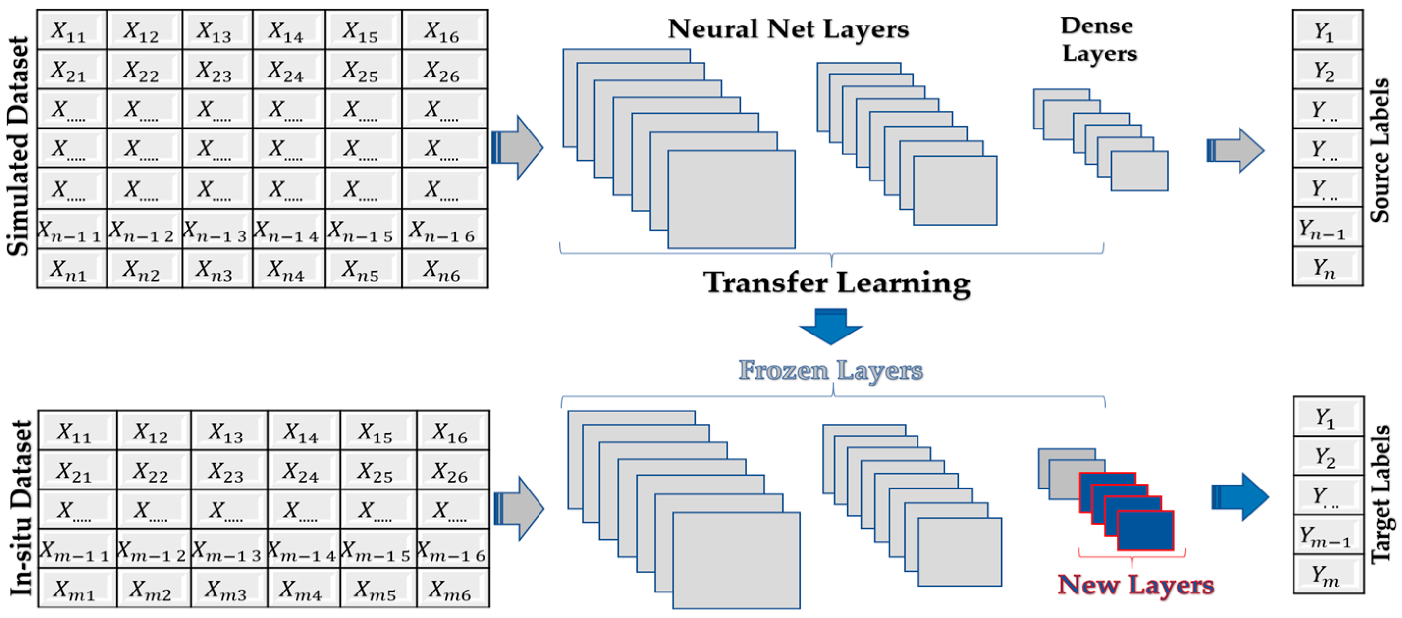
In the SFTL branch, NN models—TrF, DNN, and CNN—and tree-based models—RF and LGBM—are pre-trained on a large, simulated dataset (70% training, 30% testing) using KFold cross-validation to optimize hyperparameters. These pre-trained models are then fine-tuned on two high-quality in situ datasets (Heihe: 54 samples; Huailai: 238 samples), which are split into 60% training, 15% evaluation, and 25% testing subsets. A suite of adaptation strategies—including full fine-tuning, head-only tuning, gradual layer-wise updates, adapter modules, and LoRA—is applied to enhance model generalization while minimizing computational overhead. Both procedures are rigorously validated against the in situ datasets, with performance metrics (RMSE, R2, and bias) compared across pathways. The flowchart (Figure 2) illustrates how these dual strategies are ultimately compared and then discussed to highlight their complementary strengths in LST retrieval.

3.1. Transfer-Learning and SFTL Framework

As illustrated in Figure 2a, SFTL-based models form the core of this study’s framework for retrieving LST from high-resolution VIMI data. The process of enhancing performance on a new task by leveraging knowledge gained from a related task is known as TL (Figure 3) [43,55]. When the extracted features are general—meaning they are relevant to both the base and target tasks rather than unique to the source domain—TL is more likely to succeed [56]. Although most machine learning models are traditionally designed for single-task scenarios [57], there is growing interest in developing algorithms that support knowledge transfer across domains [46,47]. In the remote sensing field, this often involves pre-training a model on a simulated dataset or image and improving its performance in another through fine-tuning or transfer-based strategies for tree-based models [58]. This approach is especially valuable when working with small in situ datasets like those from Heihe and Huailai, as it enhances generalization without requiring extensive new data [59]. Therefore, as explained in the following sections, we implemented both pre-training—on a simulated dataset—and fine-tuning (or knowledge transfer)—on the two in situ datasets—as key steps in our framework (Figure 2a). Moreover, to mitigate the risk of overfitting during both stages and to improve model stability and overall performance, we employed 5-fold cross-validation and early stopping techniques.

3.1.1. Pre-Training Process

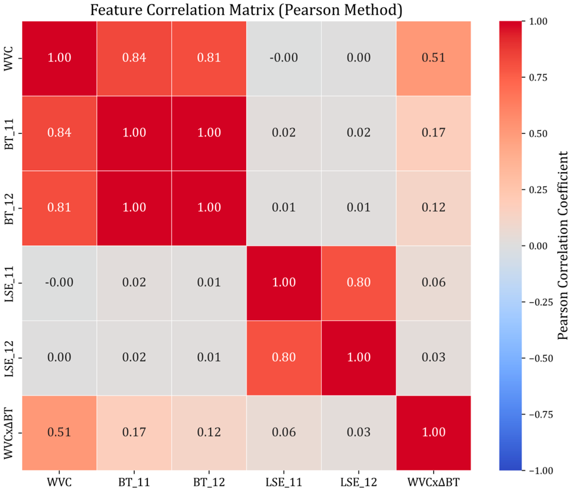
Before evaluating model performance, we examined the interrelationships among the six input variables in the simulated dataset using the Pearson correlation coefficient (Figure 4). The analysis revealed a strong positive correlation between WVC and the BTs of channels 11 and 12 (BT_11: r = 0.84, BT_12: r = 0.81), as well as a nearly perfect correlation between BT_11 and BT_12 (r ≈ 1.00), reflecting their shared spectral characteristics in the thermal infrared region. LSEs (LSE_11 and LSE_12) also exhibited a high mutual correlation (r = 0.80) but showed negligible correlation with WVC and BTs, indicating their relative independence from atmospheric water vapor effects. The engineered feature WVC × ΔBT demonstrated moderate correlation with WVC (r = 0.51) and low correlation with BT_11 and BT_12, suggesting it contributes unique information that is not fully captured by the original variables. This low-to-moderate redundancy among variables supports their joint use in the retrieval framework, with the engineered feature potentially enhancing model generalization across varying atmospheric and surface conditions.
The results presented in this section systematically evaluate the performance of our research across four critical dimensions of LST retrieval as follows: (i) LST retrieval through traditional physics-based SW algorithms; (ii) pre-training effectiveness on the large-scale simulated dataset; (iii) cross-regional adaptation capability through strategic fine-tuning; and (iv) real-world applicability to GF5-02 VIMI imagery.
In the pursuit of precise LST prediction using TIR satellite data, the pre-training stage serves as the cornerstone of our SFTL framework [43]. This foundational phase marks the beginning of the model’s learning process—capturing the core patterns and relationships essential for accurate LST estimation [60]. By incorporating a feature-engineered variable and fostering a broad, generalized understanding of LST dynamics, we directly address three persistent challenges in remote-sensing-derived LST: limited input variables, data scarcity, and regional variability. The objective is to equip the models for effective adaptation to the complexities of real-world environmental conditions. To this end, our approach employs five distinct machine learning models, each selected for its ability to capture different aspects of LST variability and to provide comparative insights as follows: (I) TrF [43,61], (II) DNN [11,43,62], (III) CNN [41,63,64], (IV) RF [63,64], and (V) LGBM [24,60,65]. These models were chosen because they represent diverse and widely used ML architectures for LST regression, whereas more complex frameworks (e.g., U-Net, ViT, and GANs) were not included due to their need for dense labels or large datasets that are unavailable in this study.
During this stage, model hyperparameters—such as the number of hidden layers, batch size, number of heads, dropout rate, and learning rate for NNs, as well as the number of estimators, maximum depth, number of leaves, and related parameters for tree-based models—are optimized using a grid search CV function [60]. Each model is then trained on the simulated dataset using a 5-fold CV, incorporating five core variables: water vapor content (WVC), brightness temperature (BT), and land surface emissivity (LSE) for channels 11 and 12 of the VIMI sensor, along with a feature-engineered variable, WVC × ΔBT (i.e., WVC divided by the BT difference between channels 11 and 12) (Table 3).

3.1.2. Fine-Tunning

Theoretically, TL manifests differently across model architectures due to their distinct mathematical foundations. In NNs, it operates in a continuous parameter space via gradient-based optimization, enabling approaches such as feature extraction and various fine-tuning strategies [46,47,48]. In contrast, tree-based models function within a discrete decision space, where TL involves structural or instance-based adaptations—such as structural modifications (STRUT), threshold adjustments (SER) [64], or instance reweighting methods like TrAdaBoost [66,67]—rather than continuous parameter updates [47]. While our study primarily focuses on NN fine-tuning, we also incorporate TL in tree-based models through model-space adaptation, using pre-trained models as initialization for target domain training.
A key challenge in NN-based TL is identifying which layers to fine-tune [68]. To date, aside from a few context-specific heuristics, no universally accepted guideline exists for optimal layer selection or hyperparameter tuning [68]. Therefore, the number of lower layers to fix and higher layers to fine-tune depends largely on the similarity between source and target datasets. For closely related datasets, fine-tuning only the fully connected layers often yields satisfactory performance. In contrast, for less similar datasets, full fine-tuning may risk negative transfer (NT), and with limited labeled data in the target domain, it can lead to overfitting [43,69]. To address this, we formulated the layer selection and tuning process as an optimization problem and applied the GridSearchCV function to evaluate a diverse set of hyperparameters—learning rates, dropout rates, and regularization coefficients—and fine-tuning strategies, including the following:
-
Full fine-tuning: All network parameters are updated, providing maximum adaptation capability but risking overfitting and catastrophic forgetting with limited target data [69,70,71].
-
Head fine-tuning: It preserves the pre-trained feature extraction layers by freezing all weights except those in the final prediction head. This strategy initializes the prediction head with random weights while keeping other layers fixed [70].
-
Gradual fine-tuning: It follows a progressive unfreezing schedule, where deeper layers are incrementally activated based on validation performance [69,71].
-
Adapter fine-tuning: It freezes all pre-trained weights and updates only lightweight adapter modules inserted between layers. Each adapter consists of a down-projection layer (typically reducing dimensionality by a specified factor), a nonlinear activation function, and an up-projection layer [72,73].
-
LoRA fine-tuning: It accelerates fine-tuning by updating only low-rank decomposition matrices within each layer, significantly reducing trainable parameters while preserving adaptation capability [43,72,74].

3.2. Operational SW Algorithm

The SW algorithm utilized in this study was an improved generalized SW algorithm developed for MODIS data [1,75].
T s = C + ( A 1 + A 2 1 ε ε + A 3 Δ ε ε 2 ) T i + T j 2 + ( B 1 + B 2 1 ε ε + B 3 Δ ε ε 2 ) T i T j 2 + D ( T i T j ) 2
where T s is the LST; T i and T j are the BTs of two thermal infrared channels. ε is the average LSE of two channels, and ∆ε is the difference between the two LSEs. The core improvement of the algorithm is the introduction of the ASTER global emissivity dataset (GED) to improve the emissivity accuracy over barren surfaces in the SW algorithm [1]. Coefficient simulations were performed using the clear-sky atmospheric profiles over land in the TIGR database and the MODTRAN 5.2. In the SW algorithm, two neighboring TIR bands are used to remove atmospheric interferences because of their diverse atmospheric absorption [4,76]. Thus, based on that theory, channels 11 and 12 of the VIMI sensor are taken into account to examine the mentioned algorithm.

LSE Estimation

Surface emissivity quantifies how effectively a surface emits heat as radiant energy outward. This property is primarily determined by the surface’s material composition, texture, and physical characteristics, such as moisture content. Additionally, its behavior varies across different wavelengths depending on the surface’s material properties and structural attributes. Understanding emissivity enables the differentiation—and in some cases, identification—of distinct surface types, while also serving as a critical factor in calculating surface temperatures [76,77]. To obtain the LSE, the Vegetation Cover Method (VCM) was utilized [52], which takes each pixel into account as a mixed pixel of bare soil and vegetation. The emissivity was determined using Equation (2) by introducing the real-time vegetation fraction data.
ε i = ε i b a r e 1 f + ε i v e g   f + d ε i
where ε i v e g and ε i b a r e are the emissivity of the vegetated and bare components at the channel i , respectively. As the vegetation cover in the study area is small and the type is single, the vegetation emissivity is assigned 0.982 and 0.984 for bands 11 and 12. ƒ is the Fraction of Vegetation Cover (FVC), determined by red and near-infrared bands from VIMI data, and d ε i is the cavity term. The cavity term in Equation (2) is computed by the following:
d ε i = 4 d ε i f ( 1 f )
where d ε i is the maximum cavity effect value, which is assumed to exist under nadir observation and can be simplified as follows:
d ε i = ( 1 ε i b a r e ) ε i v e g F ( 1 f )
where F is the shape-factor in the “box model” depending on the vegetation height and separation. The emissivity of bare soil in (2) was estimated from the ASTERGED based on the following Equation (5):
ε A S T ,   b a r e   = ε A S T ε v e g     ƒ v , A S T 1 ƒ v ,   A S T
where ε A S T is the ASTER GED v3 emissivity, ε A S T , b a r e and ε v e g is the ASTER bare and vegetation component emissivity, and f v , A S T is the ASTER vegetation coverage. In GED v3 data, pixels with FVC greater than 0.9 have the mean emissivity of 0.972, 0.971, 0.969, 0.974, and 0.974 for the five ASTER TIR channels, respectively. To this end, samples of bare soil emissivity are selected from the ASTER emissivity library, and then the bare soil emissivity of the corresponding channel of the sensor is obtained by convolution of the spectral response function and the bare soil emissivities. The bare soil emissivity of VIMI is calculated using the bare soil emissivity of the ASTER five channels through the following Equation (6):
ε i   = c 0 + c 1 ε 10 + c 2 ε 11 + c 3 ε 12 + c 4 ε 13 + c 4 ε 14
where ε i is the VIMI band emissivity, ε 10 ~ ε 14 are the five ASTER band emissivities, and c 0 ~ c 5 are the coefficients estimated by regression.

3.3. Accuracy Metrics and Sensitivity Analysis

Four statistical metrics were used to evaluate model performance: the coefficient of determination (R2), root mean square error (RMSE), mean absolute percentage error (MAPE), and bias (BIAS). R2 measures the proportion of variance in observed LST values explained by the model predictions and is defined as follows [11,60,63]:
R 2 = 1 i = 1 n L S T T r u e i L S T P r e d i 2 i = 1 n L S T T r u e i L S T ¯ 2
RMSE quantifies the magnitude of average prediction errors, giving greater weight to larger errors due to squaring the following:
RMSE = 1 n i = 1 n L S T T r u e i L S T P r e d i 2  
MAPE expresses prediction accuracy as an average percentage error, allowing normalized comparisons across datasets as follows:
MAPE = 100 n i = 1 n L S T P r e d i L S T T r u e i L S T T r u e i
BIAS measures the average tendency of predictions to overestimate or underestimate the true values as follows:
BIAS = 1 n i = 1 n L S T P r e d i L S T T r u e i  
For each model, prediction errors (residuals) were computed, and samples with extreme deviations were progressively excluded. Through the following threshold determination protocol, a stable residual threshold was then determined, ensuring that at least 90% of samples were retained while minimizing metric fluctuations.
τ M , D = τ a r g m i n D D f i l t e r e d ( τ ) 0.9       S u b j e c t t o :     s k w n e s s r i τ < ε
where D f i l t e r e d = i D | r i τ M , D denotes the subset of data points retained within the threshold, r i = y ^ i y i is residual (predicted error for each sample i in dataset D ), and ε is a small constant ensuring residual distributional balance. Then, performance metrics (RMSE and R2) were recalculated on the filtered datasets, allowing us to evaluate how outlier handling influences model stability and real-world applicability.
R M S E f i l t e r e d = 1 D f i l t e r e d i D f i l t e r e d r i 2  
R f i l t e r e d 2 = 1 i D f i l t e r e d y i y ^ i 2 i D f i l t e r e d y i y ^ f i l t e r e d 2
where y ^ f i l t e r e d is the mean of observed values in D f i l t e r e d .

4. Results

4.1. The SW Algorithm and ML Models LST Retrieval

For the physical-based LST retrieval, the simulated coefficients of the SW algorithm demonstrated high accuracy. The largest RMSE was 1.20 K in the [5–6.5] water vapor content sub-interval, while the smallest error was 0.085 K in the [0–1.5] sub-interval. The operational SW algorithm was then applied to retrieve LST values using ground-measured datasets from the Huailai and Heihe sites (2021–2023). As shown in Figure 5a, the Huailai retrievals aligned well with in situ measurements, yielding an overall MAE of 2.65 K and RMSE of 3.67 K. Similarly, the Heihe retrievals showed comparable performance, though less robust due to the smaller in situ dataset, with an overall bias of 3.64 K and RMSE of 4.22 K. These results confirm the SW algorithm’s effectiveness for high-resolution LST retrieval, particularly in regions with sufficiently large in situ datasets such as Huailai.
The direct training of neural network (NN) and tree-based models on each in situ dataset demonstrated promising performance for LST retrieval. For the Heihe dataset, the DNN model outperformed all others, achieving an RMSE of 2.19 K (Figure 5b). In contrast, for the Huailai dataset, tree-based models delivered superior performance compared to NN models, although the latter still achieved competitive accuracy (Figure 5c). However, when evaluated for cross-site generalizability, performance degraded substantially, with RMSEs exceeding 4.17 K on the Heihe dataset and 4.87 K on the Huailai dataset. These results highlight an important limitation: while machine learning models exhibit strong accuracy when directly trained and tested on the same in situ dataset, their reliability diminishes under domain shift, limiting their utility for generalized LST retrieval across heterogeneous environments such as the Huailai region.

4.2. Pre-Training on the Simulated Dataset

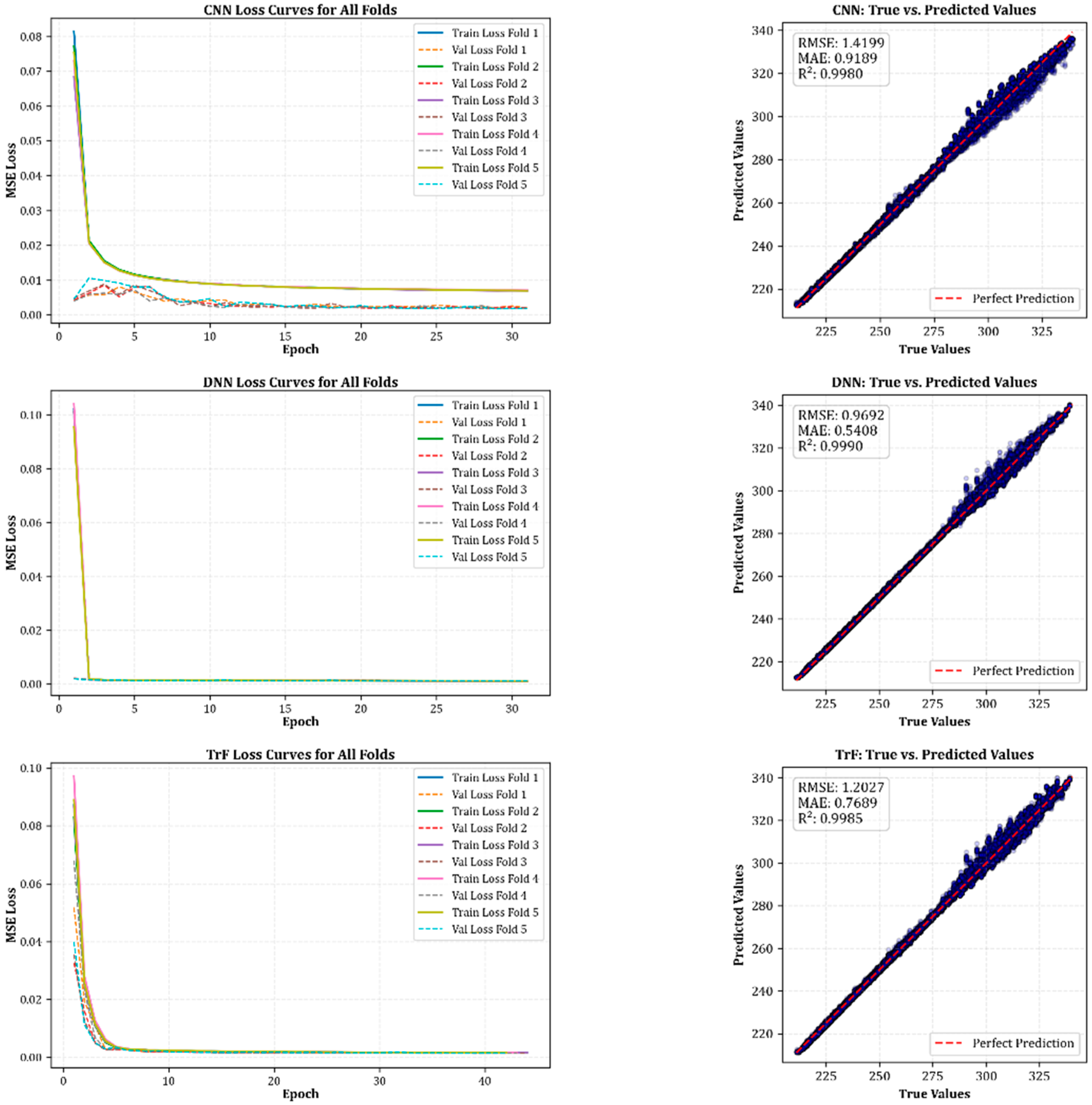
Following the physics-based baseline, we evaluated the pre-training stage of the SFTL framework using the large-scale simulated dataset. This phase is intended to equip models with a broad understanding of LST–atmosphere relationships prior to exposure to site-specific conditions, enabling more effective transfer during fine-tuning. Figure 6 shows the training and validation loss trajectories for the TrF, DNN, and CNN models across all folds. In all cases, MSE losses decreased sharply within the first 5–8 epochs, reflecting rapid convergence as dominant patterns in the simulated dataset were captured. After this initial phase, the curves plateaued, indicating that the models reached stable optima with minimal further improvement. The close alignment between training and validation losses across folds demonstrates strong generalization and the absence of overfitting, aided by the 5-fold CV scheme and early stopping. The corresponding true vs. predicted value plots confirm this high predictive accuracy, with all three NN architectures showing tight clustering along the 1:1 line. RMSE values were low (CNN: 1.419 K, DNN: 0.969 K, TrF: 1.202 K), and R2 values exceeded 0.998, underscoring the models’ ability to reproduce the simulated LST with near-perfect fidelity. These results confirm that the pre-training stage successfully captures the core relationships between thermal radiance, atmospheric properties, and LST, providing a strong foundation for subsequent fine-tuning on in situ datasets.
As summarized in Table 4, all models demonstrated strong predictive skill, with CV R2 values exceeding 0.997 for NNs and 0.9999 for RF. Among the NN models, DNN achieved the lowest average CV RMSE (0.97 K) and the highest CV R2 (0.9990), followed closely by TrF (1.21 K, 0.9980). CNN exhibited slightly higher errors (CV RMSE = 1.42 K) but maintained strong generalization (CV R2 = 0.9980). For tree-based learners, RF delivered the best overall performance (RMSE = 0.296 K, R2 = 0.9999), with LGBM ranking second (test RMSE = 0.410 K, R2 = 0.9998).
Permutation feature importance analysis revealed consistent patterns across model types. For NN models, BT_11, BT_12, and the engineered feature WVC × ΔBT emerged as the top predictors, highlighting the value of feature engineering in capturing subtle interactions between atmospheric water vapor content and inter-channel brightness temperature differences. In contrast, tree-based models prioritized BT_11, BT_12, and WVC. This convergence in key predictors suggests that the simulated dataset effectively encapsulated the spectral–atmospheric relationships governing LST variability.

4.3. Fine-Tuning and Cross-Domain Generalization

Following pre-training on the large-scale simulated dataset, the SFTL framework was fine-tuned on two in situ datasets—Heihe and Huailai—using five NN adaptation strategies alongside model transfer for tree-based learners. This stage aimed to assess cross-regional adaptability and the effectiveness of parameter-efficient tuning methods in enhancing predictive accuracy and examining the cross-site generalization of LST retrieval under domain shifts between two field sites with markedly different sample sizes. Model selection was performed using validation RMSE, with warm-up + cosine scheduling and early stopping applied for neural models. Additionally, the TrF was optimized with layer-wise learning-rate decay. Evaluation metrics included RMSE, MAE, R2, and MAPE, calculated robustly under an interquartile range (IQR) mask (k = 1.5) on residuals. A dedicated sensitivity analysis varied this multiplier between 0.5 and 4.0 to assess the stability of conclusions, and residual distributions were visualized using IQR-filtered boxplots. Finally, two symmetric experiments were conducted as follows: (i) fine-tune/test on Huailai → test on Heihe and (ii) fine-tune/test on Heihe → test on Huailai.

4.3.1. Fine-Tuning on Huailai → Generalization to Heihe

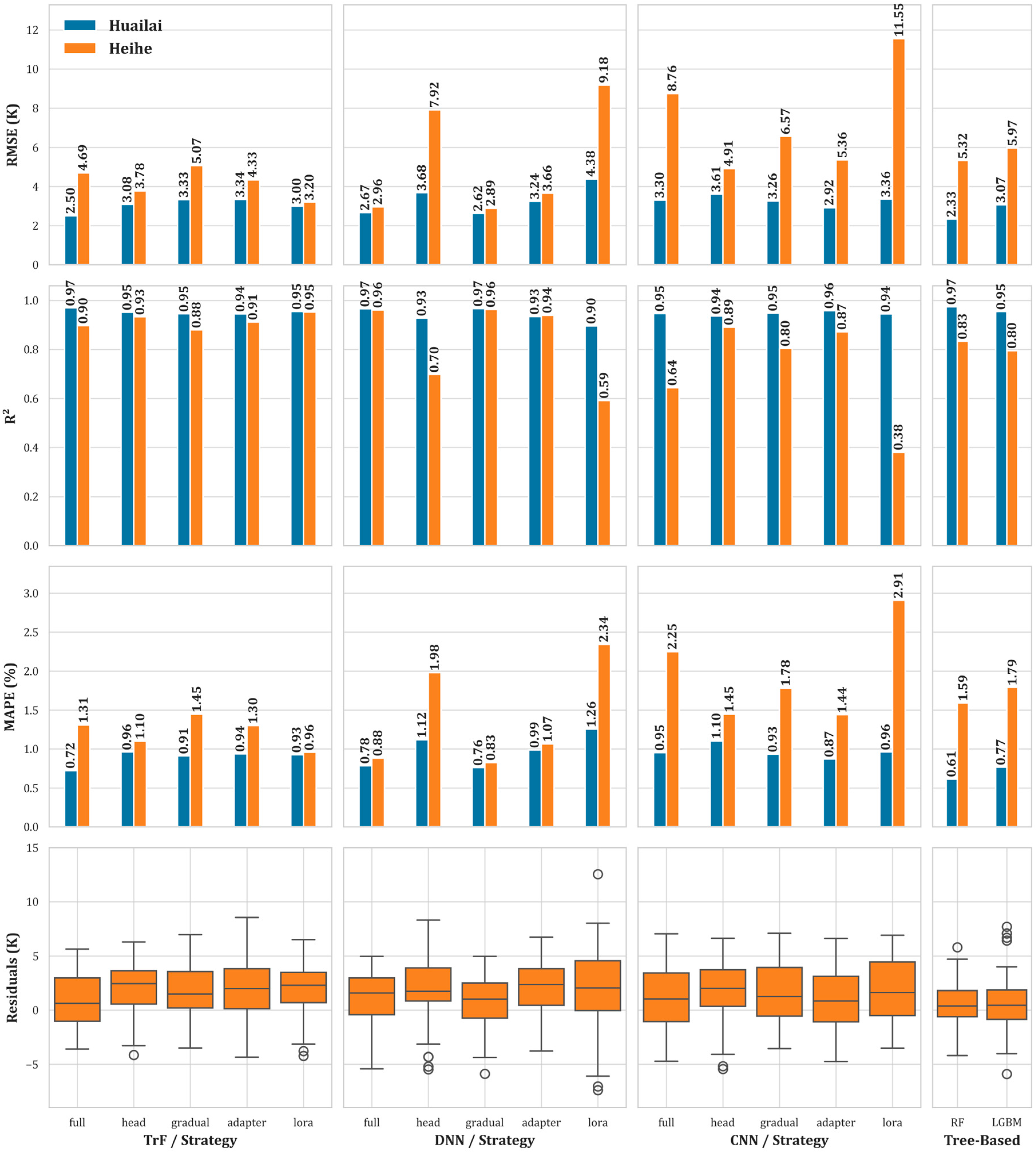
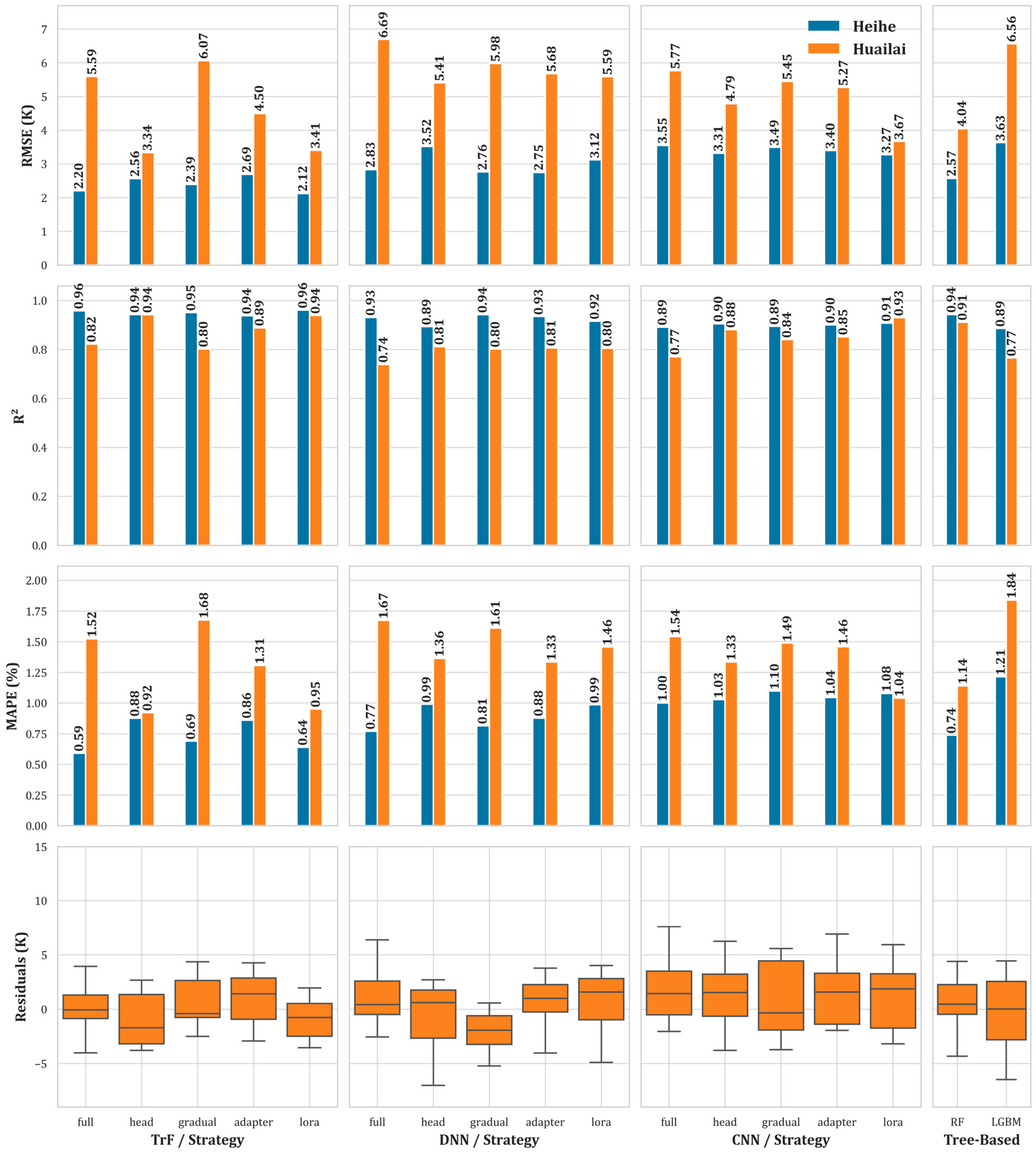
As illustrated in Figure 7 and summarized in Table 5, in the SiHuHe scenario, results revealed substantial variability in performance across strategies and architectures. With the larger source dataset (Huailai, n = 235), gradual unfreezing of the DNN provided the most reliable cross-site skill. The best DNN-gradual configuration achieved RMSE ≈ 2.62 K on the Huailai test split and ≈ 2.89 K on Heihe.
In the ablation figure centered on Huailai fine-tuning, the orange bars (Heihe) for DNN-gradual are the lowest among all strategies and backbones; the R2 and MAPE panels show the same trend, and the Huailai residual boxplots remain tight and centered near zero after IQR filtering. Closely following were DNN-full and the parameter-efficient DNN-adapter, posting in-domain RMSEs of ≈2.67 K and 3.24 K on Huailai and cross-site RMSEs of ≈2.96 K and 3.66 K on Heihe, respectively. This outcome is consistent with transfer-learning theory: with a sufficiently large source, gradually increasing model capacity allows later layers to adapt to site-specific feature–target mappings while earlier layers retain generalizable structure.
For sufficiently large target domains (Huailai, n = 235), this avoids both under-adaptation (head-only tuning) and over-specialization (immediate full unfreezing), resulting in stronger cross-site generalization. By contrast, TrF variants fine-tuned on Huailai generalized less effectively to Heihe (e.g., head/LoRA RMSE ≈ 3.78–3.20 K), while CNN strategies performed even worse for cross-site transfer in this direction (≈4.91–11.55 K). Tree-based baselines further accentuate the point: although RF and LGBM fit Huailai well (RF ≈ 2.32 K and LGBM ≈ 3.07 K), their errors increased substantially on Heihe (≈5.32 K and ≈5.97 K, respectively), reflecting over-partitioning around source-site thresholds that did not hold under domain shift.

4.3.2. Fine-Tuning on Heihe → Generalization to Huailai

In the SiHeHu scenario, our exploration began with the Heihe dataset as the source for fine-tuning, testing its ability to transfer knowledge to Huailai—a classic cross-site challenge in remote sensing, where atmospheric, topographic, and land cover differences test model robustness.
The results, as detailed in Table 6, illuminate a reversal in optimal strategies compared to larger-source scenarios. Head-only fine-tuning of the TrF model emerged as a standout, achieving an in-domain RMSE of approximately 2.56 K on Heihe while demonstrating exceptional cross-site generalization to Huailai with an RMSE of ~3.34 K. This approach, which focuses updates solely on the output head while freezing the feature extractor, preserves the rich representations learned from simulations, avoiding the pitfalls of over-adaptation on limited samples. In the ablation figure centered on Heihe fine-tuning (Figure 8), the orange bars (Huailai) for TrF-head are consistently the lowest across all strategies and backbones; the R2 and MAPE panels show the same trend, and the Heihe residual boxplots remain compact and centered near zero after IQR filtering. Closely following were parameter-efficient methods like TrF-LoRA and CNN-LoRA, posting in-domain RMSEs of ~2.12 K and 3.27 K on Heihe, respectively, and cross-site RMSEs of ~3.41 K and 3.67 K on Huailai. These techniques, by introducing lightweight adapters or low-rank matrices, enable targeted updates that enhance transfer without destabilizing the pre-trained backbone—a critical advantage when source data is small, as full fine-tuning (e.g., TrF-full at Heihe RMSE ~2.20 K but Huailai ~5.59 K) often leads to higher cross-site errors due to overfitting [73] and particularly when weighty differences exist between source and target domain distributions, potentially resulting in NT [74].
This pattern underscores a broader theme: in small-source domains, restraint breeds resilience. While full or gradual fine-tuning excelled in-domain—yielding low Heihe RMSEs like TrF-gradual (~2.39 K), DNN-gradual (~2.76 K), and RF (~2.57 K)—their generalization to Huailai suffered, with RMSEs climbing to 6.07 K, 5.98 K, and 4.04 K, respectively. Tree-based models like RF and LGBM, though efficient and yielding solid in-domain performance (Heihe RMSE ~2.57 K and 3.63 K), similarly struggled cross-site (Huailai ~4.04 K and 6.56 K), highlighting the limitations of ensemble methods without the inductive biases of neural architectures in transfer scenarios. Sensitivity analysis further bolsters this narrative, showing that the RMSE distributions for head and LoRA strategies stabilize at lower values across IQR multipliers (e.g., mean RMSE ~2.56–3.41 K at stable multipliers of 1.0–1.5), indicating robust performance even under varying outlier thresholds—a proxy for real-world noise tolerance. Ultimately, this story of adaptation in scarcity reveals that for LST models navigating the sim-to-real gap with limited in situ data, parameter-efficient fine-tuning—epitomized by TrF-head, TrF-LoRA, and CNN-LoRA—offers a path to superior generalizability. By minimizing updates to preserve simulated knowledge, these methods not only achieve competitive in-domain accuracy but also excel in cross-site transfer, paving the way for more reliable LST estimation in data-constrained regions. Future work could explore hybrid strategies or domain randomization in simulations to further bridge these gaps, ensuring models thrive beyond the confines of their training origins.

5. Validation

This section consolidates the evidence that the proposed SFTL retrieves reliable GF5-02/VIMI LST in two contrasting regions (Huailai and Heihe). Validation proceeds in the following four escalating cases:
(I) 
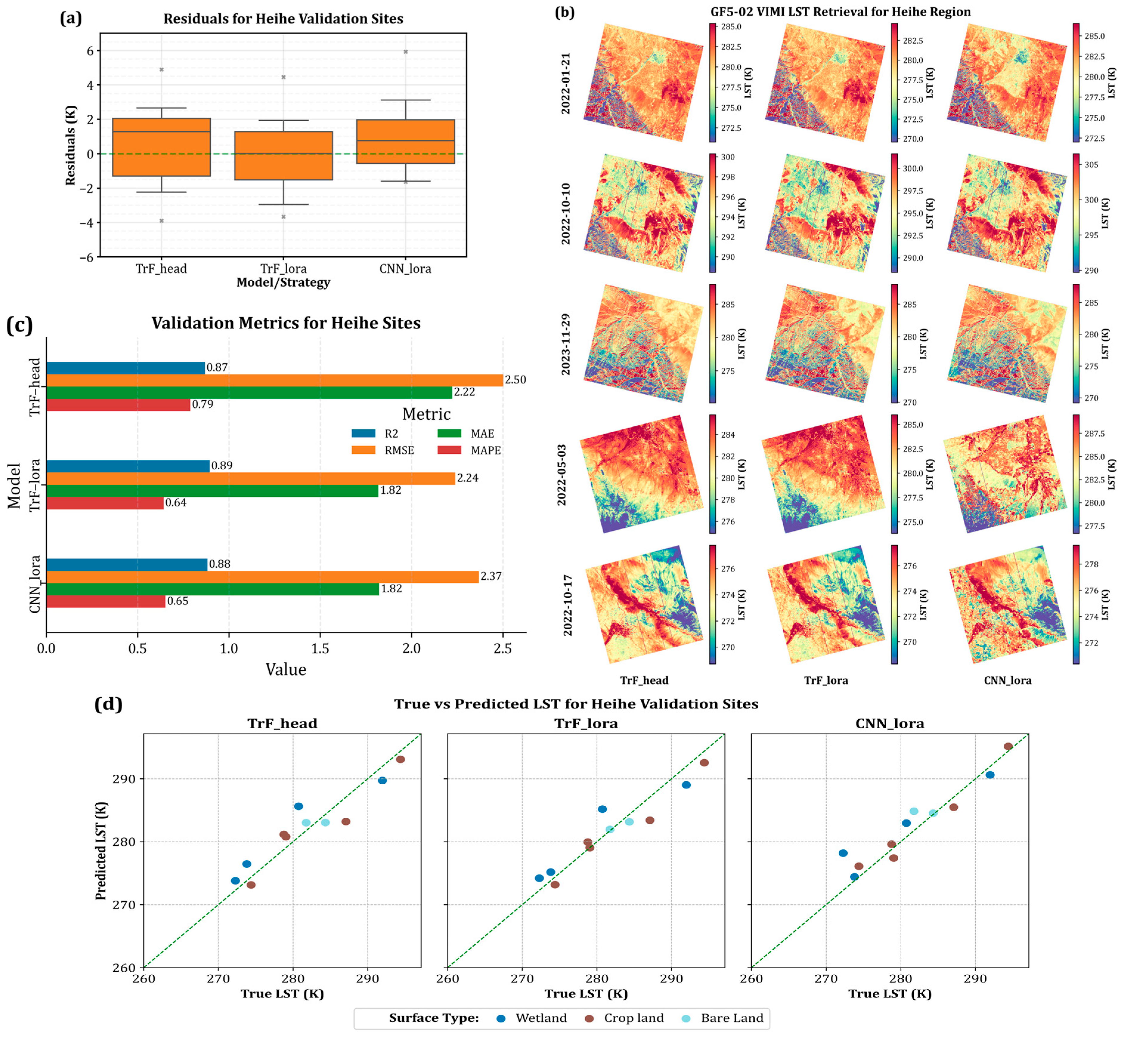
Real image LST retrieval: The GF5-02/VIMI thermal images at the Huailai and Heihe sites were used for validating real image LST retrieval, focusing on the strongest model–strategy configurations per site and their agreement with co-located, time-matched in situ observations (Figure 9 and Figure 10 describe residual distributions, five date-specific LST maps, aggregated site-level metrics, and pointwise true–predicted agreement by surface type). For Huailai, the DNN with gradual unfreezing and full fine-tuning emerged as the leading strategies, followed by TrF-LoRA and head-only fine-tuning. Gradual unfreezing DNN achieves RMSE = 2.66 K, R2 = 0.96, MAE = 2.24 K, and MAPE = 0.80%, with a bias of +1.76 K over 71 validation samples; the fully fine-tuned DNN is slightly lower on RMSE (2.91 K) and R2 (0.95) with the close MAE (2.45) and MAPE (0.88%), and a comparable bias of +2.13 K across 71 samples. These two configurations therefore deliver sub-3 K errors with >0.95 explained variance in operational imagery while maintaining near-zero median residuals, which is consistent with the tight, symmetric residual boxplots and the near-1:1 scatter evident in Figure 9d. Other strong baselines—TrF-LoRA (RMSE = 3.27 K; R2 = 0.93) and TrF-head (3.5 K; 0.92)—remain competitive. However, gradual unfreezing and full fine-tuning for sufficiently large target domains are defensible and indicate that excessively lightweight adaptation can underfit the radiative variability present in real scenes (Table 7).
It is worth noting that in a few Huailai stations, such as Corn5, both SFTL- and SW-derived LSTs show a noticeable warm bias relative to in situ observations. Visual inspection of high-resolution VIMI imagery and land-cover maps indicates that Corn5 lies near field boundaries and mixed surfaces, such that the 40 m VIMI footprint captures a mixture of crops and adjacent land covers, whereas the ground radiometer samples only a small homogeneous patch. This spatial-representativeness mismatch between the satellite pixel and the point-scale station is therefore the primary cause of the local bias, with any residual geo-location offset (≤one pixel) contributing only secondarily.
For Heihe, the TrF with LoRA attains the best real-image performance (RMSE = 2.24 K, R2 = 0.89, MAE = 1.82 K, MAPE = 0.64%, bias = −0.14 K; n = 11), followed closely by CNN-LoRA (RMSE = 2.37 K, R2 = 0.88, MAE = 1.82, MAPE = 0.65%, bias = 0.99 K). Both models exhibit minimal bias with narrow residual interquartile ranges and tight alignment to the 1:1 line across surface types in Figure 10d. The negative biases (−0.14 K) suggest a slight cool tendency, but they are small relative to the overall error budget. The spatiotemporal validation—residual boxplots, five-date LST maps, site-level bar metrics, and per surface scatter—collectively supports the robustness of these top configurations. The maps across five acquisition dates show consistent spatial gradients and thermal contrasts that are physically plausible for each landscape, while the bar metrics consolidate performance across dates and stations, yielding R2 values > 0.88 and MAPE < 1.17% for the best strategies at both sites. The scatter panels further indicate that agreement is maintained across diverse surface classes, with departures concentrated at the hottest and coolest extremes where emissivity and atmospheric correction uncertainties are inherently larger (see the organization of panels and their purpose in Figure 9 and Figure 10).
The evidence points to two consistent themes. First, partial fine-tuning that preserves pre-training while exposing a small number of task-critical parameters (DNN-gradual; TrF-LoRA/head; CNN-LoRA) yields the most reliable real-image performance on both sites. Second, bias control is excellent: all leading models maintain absolute bias ≲3.03 K in Huailai and <0.99 K in Heihe, aligning with the near-symmetric residual distributions in the validation panels (Figure 9a,c,d and Figure 10a,c,d). Together, these outcomes demonstrate that the proposed transfer-learning strategies translate from simulation-trained models to operational GF5-02/VIMI imagery with site-specific realism while retaining generalization across distinct surface and atmospheric regimes. Moreover, with RMSE around 2.24–3.5 K and R2 ≈ 0.88–0.96 in real acquisitions—supported by spatiotemporally matched in situ data and consistent spatial patterns across dates—the study’s best configurations meet the accuracy required for many land-surface process applications and provide a credible pathway for routine LST retrieval from GF5-02/VIMI over heterogeneous landscapes. The comparative shortfall of DNN-Adapter tuning in Huailai underscores the importance of selecting an adaptation depth commensurate with scene complexity and available ground truth.
(II) 
Within-site fidelity and cross-site generalization: Fine-tuning on the larger Huailai dataset (≈235 valid samples after physically screening LST ranges) yields consistently low errors on its hold-out set and, crucially, transfers well to Heihe. Among neural strategies, DNN with gradual unfreezing provides the most balanced performance: RMSE ≈ 2.62 K (Huailai hold-out) and ≈2.89 K on Heihe, with R2 around 0.95 and ≈0.93, respectively. TrF-LoRA and head-tuning variants perform similarly on the Huailai holdout (RMSE ≈ 3.00–3.08 K) but are less stable on Heihe (RMSE ≈ 3.20–3.78 K). Tree-based transfer (RF/LGBM) trails the neural approaches in this direction (RMSE ≈ 5.32–5.97 K on Heihe), underscoring the benefit of a pre-trained representation that can be lightly adapted. When the direction is reversed—fine-tuning on the much smaller Heihe dataset (≈54 samples)—the models achieve excellent in-domain accuracy (e.g., TrF-LoRA ≈ 2.12 K and TrF-head ≈ 2.50 K). However, cross-site performance on Huailai is less favorable, with the best results being TrF-head at ≈3.34 K, TrF-LoRA at ≈3.41 K, and CNN-LoRA at ≈3.67 K. Tree models again degrade strongly under distribution shift (RF ≈ 4.13 K; LGBM ≈ 6.57 K). This asymmetry is consistent with sample size and distributional effects: the smaller Heihe set constrains the diversity of radiative and land-cover conditions seen during adaptation, while the richer Huailai set better regularizes the model and improves transfer. Together, the two directions reveal that (a) the pre-trained backbone retains broadly useful thermal structure and (b) the depth of adaptation matters—exposing a modest set of parameters (head-tuning, gradual unfreezing, or compact LoRA) is generally preferable to either freezing too much (adapter-only underfits) or over-specializing.
(III) 
Sensitivity to outlier filtering (IQR multiplier): To ensure robustness of the reported statistics to the outlier definition, the IQR multiplier used to mask residuals was swept from 0.5 to 4.0. Two stability properties emerge. First, for the reference range of 1.0–1.5, model rankings are unchanged and RMSE variability is typically <1%, confirming that headline conclusions are not artifacts of the threshold. Second, the “stable multiplier”—the smallest multiplier ≥1.0 that keeps RMSE within ±1% of the value at 1.5—lies at 1.0 or 1.5 for almost all model/strategy/site combinations. For example, DNN-full/gradual and TrF-LoRA-head remain stable at 1.5 in Huailai, while CNN/LoRA and TrF-LoRA/head are stable at 1.5 in Heihe. This analysis provides a quantitative guardrail: performance claims persist under reasonable, defensible choices of the residual-masking threshold and are therefore not the result of aggressive outlier trimming.

6. Discussion

The central premise of this study is that physics-aware TL can bridge the long-standing gap between radiative-transfer simulations and real scenes to retrieve LST robustly across places, seasons, and atmospheric regimes. Prior work has moved in this direction along two complementary lines: coupling expert physical knowledge with data-driven models (e.g., MDK-DL) to stabilize learning and feature selection [36] and transfer-learning pipelines that reduce reliance on ancillary inputs such as explicit emissivity by leveraging both emissive and reflective TOA signals [8]. Ensemble and hybrid models have likewise shown that injecting water–vapor-aware features tied to the radiance transfer equation improves retrieval fidelity [41]. These strands, together with broader guidance on when and how to transfer between domains in environmental sensing [43] and evidence that TL can recover accuracy under data scarcity [11], frame the design choices and evaluation logic used here.
Within this context, the SFTL framework developed in this study begins with a broad RTM-generated source domain and subsequently fine-tunes on site-specific data. A key component is the feature-engineered variable WVC × ΔBT, designed to capture humidity-driven channel contrast in the atmospheric window. This variable proved pivotal in the TrF pre-training step, where its removal increased RMSE by 6.845 K and reduced R2 by 0.062. Its importance is consistent with prior findings: MDK-DL studies have shown that accurate water-vapor information substantially improves LST retrieval [36], and ensemble-based evidence demonstrates that a water-vapor index coupled with TOA brightness temperature reduces errors by explicitly encoding radiance–transfer dependencies [41]. The ablation experiments conducted here reinforce these insights, showing that excluding WVC × ΔBT degrades performance across all metrics—particularly under moist, mid-latitude conditions—mirroring the underlying physics that motivated the feature’s construction.
Generalizability was then assessed by deliberately reversing the transfer direction across two independent sites—Heihe and Huailai—via two SiHuHe and SiHeHu pipelines. In both directions, the generalization gap remained small relative to the within-site fine-tune performance, and error distributions stayed tight when evaluated against spatiotemporally collocated in situ LST. This pattern is exactly what would be expected if the pre-trained backbone were learning transportable radiative-transfer structure and the WVC × ΔBT term were neutralizing site-specific humidity differences at inference. It also aligns with the documented advantages of TL for geophysical mapping across heterogeneous regions: transferring “core” representations from data-rich to data-scarce domains reduces the amount of target-domain data required while preserving accuracy [11,43].
The sensitivity analysis clarifies why the strategy works and how to deploy it. First, model-capacity tests show the backbone can be partially frozen without sacrificing accuracy; selectively unfreezing later blocks during fine-tuning yielded the best trade-off between stability and domain adaptation, consistent with TL practice in environmental remote sensing and with empirical sensitivity to “freezing layers” reported in related TL studies [11,43]. Second, feature-importance and perturbation tests confirm that WVC × ΔBT is among the most influential predictors in humid atmospheres and that its contribution persists after controlling for ΔBT alone—again in line with physics-guided modeling [36,41]. Finally, robustness checks (including outlier-handling thresholds) indicate that the improvements are not artifacts of filtering; performance trends are stable across reasonable IQR multipliers, with the largest resilience gains appearing in the high-WV tail where split-window baselines often degrade [64].
Real-image tests using GF5-02 VIMI further substantiate external validity. Retrieved LST fields exhibit coherent spatial organization across land-cover mosaics, with no systematic striping or adjacency artifacts, and station-by-station comparisons remain consistent across seasons. The results are in line with previous GF5-based LST developments and improvements via calibration and physics-aware learning, e.g., [35,36,37], while our SFTL design reduces reliance on ancillary emissivity inputs, echoing the recent TL approach that leverages both reflective and emissive TOA bands [8].
Against established baselines, the combined evidence from cross-site transfer, sensitivity analyses, and real-scene validation supports three conclusions. First, pre-training on a wide, physically diverse simulation space, followed by strategic fine-tuning, yields LST estimates that travel well between sites with distinct atmospheric water-vapor regimes—precisely the use case where classical SC/SW algorithms are most fragile [8,41]. Second, explicitly encoding humidity effects via WVC × ΔBT operationalizes the “model-data-knowledge” principle, converting radiative-transfer understanding into a compact feature that consistently improves accuracy and robustness [36,41]. Third, SFTL’s efficiency—strong performance with limited site-specific samples and partial layer freezing—matches broader lessons from environmental TL about achieving high accuracy under data scarcity while minimizing NT [11,43].
Two limitations suggest clear paths forward. First, while the bidirectional Heihe–Huailai experiments are stringent, broader multi-site, multi-sensor trials (including view-angle extremes) would better bound any residual domain shift, in keeping with calls for richer validation designs in recent LST work [41]. Second, automated transferability diagnostics (e.g., pre-transfer scoring of source–target compatibility) could make SFTL deployment more predictable at scale, echoing current best practice in TL applications for Earth observation [43]. Overall, the story that emerges is cohesive: a physics-guided TL backbone, anchored by a humidity-aware feature, transfers cleanly between contrasting North China sites, produces stable gains under sensitivity stress tests, and scales to real GF5-02 VIMI imagery with spatiotemporal validation against in situ records. In combination with the recent literature, these findings position SFTL as a practical and scientifically defensible route to publishable LST mapping that is both accurate and generalizable.

7. Conclusions

This study introduces and validates a physics-aware SFTL framework for LST retrieval. The framework begins with a broad radiative-transfer simulation space, integrates domain knowledge via the humidity-sensitive feature WVC × ΔBT, and fine-tunes on limited site-specific data. Its performance is benchmarked against the traditional SW algorithm and against direct training of NN and tree-based learners on in situ datasets. Across two cross-site pipelines—(i) SiHuHe and (ii) SiHeHu—the framework consistently achieves accurate retrievals with only a small generalization gap relative to within-site testing.
Aside from the tree-based models, the SW algorithm, and MLs’ direct training implementations, this study evaluated 15 model–strategy combinations within the SFTL framework. Among these, two clear leaders emerged across the domain-shift scenarios, reflecting differences in diversity and size between the source (simulated), target (in situ), and cross-site (in situ) datasets. In the SiHuHe scenario, the DNN with gradual unfreezing and full fine-tuning consistently outperformed other variants. The DNN-gradual achieved RMSEs of ≈2.62/2.89 K (in-site/cross-site), R2 ≈ 0.97/0.96, and MAPE ≈ 0.76/0.83%, while DNN-full delivered RMSEs of ≈2.67/2.96 K, R2 ≈ 0.97/0.96, and MAPE ≈ 0.78/0.88%. These results underscore the strength of strategies that utilize nearly all parameters of the pre-trained architecture when the target domain is sufficiently large and heterogeneous, enabling deeper layers to adapt while preserving generalizable structures. By contrast, in the SiHeHu scenario, lightweight, parameter-efficient strategies proved more effective. Attention-based and convolutional configurations—TrF-head, TrF-LoRA, and CNN-LoRA—achieved strong cross-site performance without sacrificing in-domain accuracy. TrF-head attained RMSEs of ≈2.56/3.34 K (in-site/cross-site), R2 ≈ 0.94/0.94, and MAPE ≈ 0.88/0.92%; TrF-LoRA achieved ≈2.12/3.41 K, R2 ≈ 0.96/0.94, and MAPE ≈ 0.64/0.95%; and CNN-LoRA scored ≈ 3.27/3.67 K, R2 ≈ 0.91/0.93, and MAPE ≈ 1.08/1.04%. The promising performance of these lightweight methods stems from freezing pre-trained model weights while injecting trainable low-rank decomposition matrices into each layer, which drastically reduces the number of trainable parameters.
Two practical lessons emerge. First, selective unfreezing (e.g., head, LoRA, or gradual strategies) often matches or exceeds full fine-tuning, suggesting that SFTL can be both data-efficient and stable—an important consideration for regions with sparse ground truth. Second, while purely data-driven neural backbones (TrF/DNN/CNN) show the strongest bidirectional generalization after SFTL, a physics-informed SFTL and tree-based baselines (RF, LGBM) remain competitive in-domain and serve as robust reference models for operational deployment.

Author Contributions

Conceptualization, P.H. and H.L.; methodology, P.H., H.L. and Y.T.; software, P.H. and Z.Z.; validation, P.H. and H.L.; formal analysis, H.L.; investigation, H.L. and Y.T.; resources, H.L.; data curation, H.L.; visualization, P.H. and Z.Z.; writing—original draft preparation, P.H. and Z.Z.; writing—review and editing, P.H., H.L., Y.T., F.Z., B.C., Y.D. and Q.L.; supervision, H.L., Y.T., B.C., Y.D. and F.Z.; project administration, H.L. All authors have read and agreed to the published version of the manuscript.

Funding

This work was supported by the National Key Research and Development Program of China under Grant 2023YFB3905801 and the National Natural Science Foundation of China under Grant 42471365.

Data Availability Statement

The simulated training dataset and the in situ observations used for validation are held by the corresponding author and are available upon reasonable request, subject to site data-use agreements and privacy constraints. Requests for these datasets, including the precise train/validation/test splits for Huailai and Heihe, should be directed to the corresponding author (lihua@aircas.ac.cn). The GF5-02/VIMI Level-1 imagery is distributed by the mission data provider and can be obtained from the official portal under the provider’s user agreement. Derived LST products generated in this study (site-level and evaluation subsets) can be shared for academic use upon request. Trained model weights, scaler parameters, and configuration files for the SFTL framework are available from the first author (peyman@buaa.edu.cn) for non-commercial research, contingent on acknowledgement of use and citation of this article.

Acknowledgments

The authors thank the field teams and site managers at the Huailai and Heihe observatories for maintaining in situ measurements used for validation and the GF5-02/VIMI mission and data distribution office for providing access to satellite imagery. The authors also acknowledge the developers and communities behind open-source tools—such as Python (v3.12.5), PyTorch (v2.4), scikit-learn (v1.5.1), and others—that supported this research. Helpful comments from colleagues during internal seminars substantially improved the clarity of the manuscript.

Conflicts of Interest

The authors declare no conflicts of interest.

References

  1. Li, H.; Li, R.; Tu, H.; Cao, B.; Liu, F.; Bian, Z.; Hu, T.; Du, Y.; Sun, L.; Liu, Q. An operational split-window algorithm for generating long-term Land Surface Temperature products from Chinese Fengyun-3 series satellite data. IEEE Trans. Geosci. Remote Sens. 2023, 61, 5004514. [Google Scholar] [CrossRef]
  2. Wang, X.; Yaojun, Z.; Yu, D. Exploring the Relationships between Land Surface Temperature and Its Influencing Factors Using Multisource Spatial Big Data: A Case Study in Beijing, China. Remote Sens. 2023, 15, 1783. [Google Scholar] [CrossRef]
  3. Adeyeri, O.E.; Folorunsho, A.H.; Ayegbusi, K.I.; Bobde, V.; Adeliyi, T.E.; Ndehedehe, C.E.; Akinsanola, A.A. Land surface dynamics and meteorological forcings modulate land surface temperature characteristics. Sustain. Cities Soc. 2024, 101, 105072. [Google Scholar] [CrossRef]
  4. Ru, C.; Duan, S.B.; Jiang, X.G.; Li, Z.L.; Huang, C.; Liu, M. An extended SW-TES algorithm for land surface temperature and emissivity retrieval from ECOSTRESS thermal infrared data over urban areas. Remote Sens. Environ. 2023, 290, 113544. [Google Scholar] [CrossRef]
  5. Li, Z.L.; Tang, B.H.; Wu, H.; Ren, H.; Yan, G.; Wan, Z.; Trigo, I.F.; Sobrino, J.A. Satellite-derived land surface temperature: Current status and perspectives. Remote Sens. Environ. 2013, 131, 14–37. [Google Scholar] [CrossRef]
  6. Li, Z.L.; Wu, H.; Duan, S.B.; Zhao, W.; Ren, H.; Liu, X.; Leng, P.; Tang, R.; Ye, X.; Zhu, J.; et al. Satellite remote sensing of global land surface temperature: Definition, methods, products, and applications. Rev. Geophys. 2023, 61, e2022RG000777. [Google Scholar] [CrossRef]
  7. Bright, R.M.; Davin, E.; O’Halloran, T.; Pongratz, J.; Zhao, K.; Cescatti, A. Local temperature response to land cover and management change driven by non-radiative processes. Nat. Clim. Change 2017, 7, 296–302. [Google Scholar] [CrossRef]
  8. Xu, S.; Wang, D.; Liang, S.; Jia, A.; Li, R.; Wang, Z.; Liu, Y. A novel approach to estimate land surface temperature from Landsat top-of-atmosphere reflective and emissive data using transfer-learning neural network. Sci. Total Environ. 2024, 955, 176783. [Google Scholar] [CrossRef]
  9. Luyssaert, S.; Jammet, M.; Stoy, P.C.; Estel, S.; Pongratz, J.; Ceschia, E.; Churkina, G.; Don, A.; Erb, K.; Ferlicoq, M.; et al. Land management and land-cover change have impacts of similar magnitude on surface temperature. Nat. Clim. Change 2014, 4, 389–393. [Google Scholar] [CrossRef]
  10. Li, Y.; Zhao, M.; Motesharrei, S.; Mu, Q.; Kalnay, E.; Li, S. Local cooling and warming effects of forests based on satellite observations. Nat. Commun. 2015, 6, 6603. [Google Scholar] [CrossRef]
  11. Wang, W.; Brönnimann, S.; Zhou, J.; Li, S.; Wang, Z. Near-surface air temperature estimation for areas with sparse observations based on transfer learning. ISPRS J. Photogramm. Remote Sens. 2025, 220, 712–727. [Google Scholar] [CrossRef]
  12. Song, L.; Ding, Z.; Kustas, W.P.; Xu, Y.; Zhao, G.; Liu, S.; Ma, M.; Xue, K.; Bai, Y.; Xu, Z. Applications of a thermal-based two-source energy balance model coupled to surface soil moisture. Remote Sens. Environ. 2022, 271, 112923. [Google Scholar] [CrossRef]
  13. Chen, J.M.; Liu, J. Evolution of evapotranspiration models using thermal and shortwave remote sensing data. Remote Sens. Environ. 2020, 237, 111594. [Google Scholar] [CrossRef]
  14. Gallego-Elvira, B.; Taylor, H.M.; Harris, P.P.; Ghent, D. Evaluation of regional-scale soil moisture-surface flux dynamics in Earth system models based on satellite observations of land surface temperature. Geophys. Res. Lett. 2019, 46, 5480–5488. [Google Scholar] [CrossRef]
  15. Alexander, C. Normalized difference spectral indices and urban land cover as indicators of land surface temperature (LST). Int. J. Appl. Earth Obs. Geoinf. 2020, 86, 102013. [Google Scholar]
  16. Masoudi, M.; Tan, P.Y. Multi-year comparison of the effects of spatial pattern of urban green spaces on urban land surface temperature. Landsc. Urban Plan. 2019, 184, 44–58. [Google Scholar] [CrossRef]
  17. Wu, C.; Li, J.; Wang, C.; Song, C.; Chen, Y.; Finka, M.; La Rosa, D. Understanding the relationship between urban blue infrastructure and land surface temperature. Sci. Total Environ. 2019, 694, 133742. [Google Scholar] [CrossRef] [PubMed]
  18. Zhou, D.C.; Xiao, J.F.; Bonafoni, S.; Berger, C.; Deilami, K.; Zhou, Y.Y.; Frolking, S.; Yao, R.; Qiao, Z.; Sobrino, J.A. Satellite remote sensing of surface urban heat islands: Progress, challenges, and perspectives. Remote Sens. 2019, 11, 48. [Google Scholar] [CrossRef]
  19. Zink, M.; Mai, J.; Cuntz, M.; Samaniego, L. Conditioning a hydrologic model using patterns of remotely sensed land surface temperature. Water Resour. Res. 2018, 54, 2976–2998. [Google Scholar] [CrossRef]
  20. Parinussa, R.M.; Lakshmi, V.; Johnson, F.; Sharma, A. Comparing and combining remotely sensed land surface temperature products for improved hydrological applications. Remote Sens. 2016, 8, 162. [Google Scholar] [CrossRef]
  21. Reyes, B.; Hogue, T.; Maxwell, R. Urban irrigation suppresses land surface temperature and changes the hydrologic regime in semi-arid regions. Water 2018, 10, 1563. [Google Scholar] [CrossRef]
  22. Bojinski, S.; Verstraete, M.; Peterson, T.C.; Richter, C.; Simmons, A.; Zemp, M. The concept of essential climate variables in support of climate research, applications, and policy. Bull. Am. Meteorol. Soc. 2014, 95, 1431–1443. [Google Scholar] [CrossRef]
  23. Dolman, A.J.; Belward, A.; Briggs, S.; Dowell, M.; Eggleston, S.; Hill, K.; Richter, C.; Simmons, A. A post-Paris look at climate observations. Nat. Geosci. 2016, 9, 646. [Google Scholar] [CrossRef]
  24. Zhang, H.; Tang, B.H.; Li, Z.L. A practical two-step framework for all-sky land surface temperature estimation. Remote Sens. Environ. 2024, 303, 113991. [Google Scholar] [CrossRef]
  25. Li, R.; Li, H.; Hu, T.; Bian, Z.; Liu, F.; Cao, B.; Du, Y.; Sun, L.; Liu, Q. Land surface temperature retrieval from sentinel-3A SLSTR data: Comparison among split-window, dual-window, three-channel, and dual-angle algorithms. IEEE Trans. Geosci. Remote Sens. 2023, 61, 5003114. [Google Scholar] [CrossRef]
  26. Mo, Y.; Xu, Y.; Chen, H.; Zhu, S. A review of reconstructing remotely sensed land surface temperature under cloudy conditions. Remote Sens. 2021, 13, 2838. [Google Scholar] [CrossRef]
  27. Duan, S.B.; Li, Z.L.; Tang, B.H.; Wu, H.; Tang, R.; Bi, Y.; Zhou, G. Estimation of diurnal cycle of land surface temperature at high temporal and spatial resolution from clear-sky MODIS data. Remote Sens. 2014, 6, 3247–3262. [Google Scholar] [CrossRef]
  28. Chen, Y.; Duan, S.B.; Ren, H.; Labed, J.; Li, Z.L. Algorithm development for land surface temperature retrieval: Application to Chinese Gaofen-5 data. Remote Sens. 2017, 9, 161. [Google Scholar] [CrossRef]
  29. Meng, X.; Cheng, J. Estimating land and sea surface temperature from cross-calibrated Chinese Gaofen-5 thermal infrared data using split-window algorithm. IEEE Geosci. Remote Sens. Lett. 2019, 17, 509–513. [Google Scholar] [CrossRef]
  30. Ye, X.; Ren, H.; Liu, R.; Qin, Q.; Liu, Y.; Dong, J. Land surface temperature estimate from Chinese Gaofen-5 satellite data using split-window algorithm. IEEE Trans. Geosci. Remote Sens. 2017, 55, 5877–5888. [Google Scholar] [CrossRef]
  31. Ye, X.; Ren, H.; Liang, Y.; Zhu, J.; Guo, J.; Nie, J.; Zeng, H.; Zhao, Y.; Qian, Y. Cross-calibration of Chinese Gaofen-5 thermal infrared images and its improvement on land surface temperature retrieval. Int. J. Appl. Earth Obs. Geoinf. 2021, 101, 102357. [Google Scholar] [CrossRef]
  32. Chen, Y.; Duan, S.B.; Labed, J.; Li, Z.L. Development of a split-window algorithm for estimating sea surface temperature from the Chinese Gaofen-5 data. Int. J. Remote Sens. 2018, 40, 1621–1639. [Google Scholar] [CrossRef]
  33. Yang, Y.; Li, H.; Du, Y.; Cao, B.; Liu, Q.; Sun, L.; Zhu, J.; Mo, F. A temperature and emissivity separation algorithm for Chinese gaofen-5 satellite data. In Proceedings of the IGARSS 2018-2018 IEEE International Geoscience and Remote Sensing Symposium, Valencia, Spain, 22–27 July 2018. [Google Scholar]
  34. Zhao, E.; Han, Q.; Gao, C. Surface temperature retrieval from Gaofen-5 observation and its validation. IEEE Access 2020, 9, 9403–9410. [Google Scholar] [CrossRef]
  35. Tang, B.H. Nonlinear split-window algorithms for estimating land and sea surface temperatures from simulated Chinese Gaofen-5 satellite data. IEEE Trans. Geosci. Remote Sens. 2018, 56, 6280–6289. [Google Scholar] [CrossRef]
  36. Wang, H.; Mao, K.; Yuan, Z.; Shi, J.; Cao, M.; Qin, Z.; Duan, S.; Tang, B. A method for land surface temperature retrieval based on model-data-knowledge-driven and deep learning. Remote Sens. Environ. 2021, 265, 112665. [Google Scholar] [CrossRef]
  37. Ren, H.; Ye, X.; Liu, R.; Dong, J.; Qin, Q. Improving land surface temperature and emissivity retrieval from the Chinese Gaofen-5 satellite using a hybrid algorithm. IEEE Trans. Geosci. Remote Sens. 2018, 56, 1080–1090. [Google Scholar] [CrossRef]
  38. Zheng, X.; Li, Z.L.; Nerry, F.; Zhang, X. A new thermal infrared channel configuration for accurate land surface temperature retrieval from satellite data. Remote Sens. Environ. 2019, 231, 111216. [Google Scholar] [CrossRef]
  39. Gillespie, A.R.; Abbott, E.A.; Gilson, L.; Hulley, G.; Jiménez-Muñoz, J.C.; Sobrino, J.A. Residual errors in ASTER temperature and emissivity standard products AST08 and AST05. Remote Sens. Environ. 2011, 115, 3681–3694. [Google Scholar] [CrossRef]
  40. Ye, X.; Ren, H.; Nie, J.; Hui, J.; Jiang, C.; Zhu, J.; Fan, W.; Qian, Y.; Liang, Y. Simultaneous estimation of land surface and atmospheric parameters from thermal hyperspectral data using a LSTM–CNN combined deep neural network. IEEE Geosci. Remote Sens. Lett. 2021, 19, 5508705. [Google Scholar] [CrossRef]
  41. Ye, X.; Hui, J.; Wang, P.; Zhu, J.; Yang, B. A Modified Transfer-Learning-Based Approach for Retrieving Land Surface Temperature from Landsat-8 TIRS Data. IEEE Trans. Geosci. Remote Sens. 2023, 61, 4411511. [Google Scholar] [CrossRef]
  42. Iman, M.; Arabnia, H.R.; Rasheed, K. A review of deep transfer learning and recent advancements. Technologies 2023, 11, 40. [Google Scholar] [CrossRef]
  43. Ma, Y.; Chen, S.; Ermon, S.; Lobell, D.B. Transfer learning in environmental remote sensing. Remote Sens. Environ. 2024, 301, 113924. [Google Scholar] [CrossRef]
  44. Tan, J.; NourEldeen, N.; Mao, K.; Shi, J.; Li, Z.; Xu, T.; Yuan, Z. Deep learning convolutional neural network for the retrieval of land surface temperature from AMSR2 data in China. Sensors 2019, 19, 2987. [Google Scholar] [CrossRef]
  45. Mao, K.; Wang, H.; Shi, J.; Heggy, E.; Wu, S.; Bateni, S.M.; Du, G. A general paradigm for retrieving soil moisture and surface temperature from passive microwave remote sensing data based on artificial intelligence. Remote Sens. 2023, 15, 1793. [Google Scholar] [CrossRef]
  46. Pan, S.J.; Yang, Q. A survey on transfer learning. IEEE Trans. Knowl. Data Eng. 2010, 22, 1345–1359. [Google Scholar] [CrossRef]
  47. Zhuang, F.; Qi, Z.; Duan, K.; Xi, D.; Zhu, Y.; Zhu, H.; Xiong, H.; He, Q. A comprehensive survey on transfer learning. Proc. IEEE 2021, 109, 43–76. [Google Scholar] [CrossRef]
  48. Niu, S.; Liu, Y.; Wang, J.; Song, H. A decade survey of transfer learning (2010–2020). IEEE Trans. Artif. Intell. 2020, 1, 151–166. [Google Scholar] [CrossRef]
  49. Fathi, M.; Arefi, H.; Shah-Hosseini, R.; Moghimi, A. Super-Resolution of Landsat-8 Land Surface Temperature Using Kolmogorov–Arnold Networks with PlanetScope Imagery and UAV Thermal Data. Remote Sens. 2025, 17, 1410. [Google Scholar] [CrossRef]
  50. Zheng, L.; Cao, B.; Na, Q.; Qin, B.; Bai, J.; Du, Y.; Li, H.; Bian, Z.; Xiao, Q.; Liu, Q. Estimation and Evaluation of 15 Minute, 40 Meter Surface Upward Longwave Radiation Downscaled from the Geostationary FY-4B AGRI. Remote Sens. 2024, 16, 1158. [Google Scholar] [CrossRef]
  51. Heidarian, P.; Li, H.; Zhang, Z.; Li, R.; Liu, Q.; Yumin, T. High-Resolution Land Surface Temperature Retrieval from GF5-02 VIMI Data using an Operational Split-Window Algorithm. In Proceedings of the IGARSS 2024-2024 IEEE International Geoscience and Remote Sensing Symposium, Athens, Greece, 7–12 July 2024. [Google Scholar]
  52. Li, H.; Li, R.; Yang, Y.; Cao, B.; Bian, Z.; Hu, T.; Du, Y.; Sun, L.; Liu, Q. Temperature-based and radiance-based validation of the collection 6 MYD11 and MYD21 land surface temperature products over barren surfaces in northwestern China. IEEE Trans. Geosci. Remote Sens. 2021, 59, 1794–1807. [Google Scholar] [CrossRef]
  53. Li, H.; Sun, D.; Yu, Y.; Wang, H.; Liu, Y.; Liu, Q.; Du, Y.; Wang, H.; Cao, B. Evaluation of the VIIRS and MODIS LST products in an arid area of Northwest China. Remote Sens. Environ. 2014, 142, 111–121. [Google Scholar] [CrossRef]
  54. Baldridge, A.M.; Hook, S.J.; Grove, C.I.; Rivera, G. The ASTER spectral library version 2.0. Remote Sens. Environ. 2009, 113, 711–715. [Google Scholar] [CrossRef]
  55. Ball, J.E.; Anderson, D.T.; Chan, C.S. Comprehensive survey of deep learning in remote sensing: Theories, tools, and challenges for the community. J. Appl. Remote Sens. 2017, 11, 042609. [Google Scholar] [CrossRef]
  56. Torrey, L.; Shavlik, J. Transfer learning. In Handbook of Research on Machine Learning Applications and Trends: Algorithms, Methods, and Techniques; IGI Global Scientific Publishing: Hershey, PA, USA, 2010; pp. 242–264. [Google Scholar]
  57. Chevallier, F.; Chéruy, F.; Scott, N.A.; Chédin, A. A neural network approach for a fast and accurate computation of a longwave radiative budget. J. Appl. Meteorol. Climatol. 1998, 37, 1385–1397. [Google Scholar] [CrossRef]
  58. Yosinski, J.; Clune, J.; Bengio, Y.; Lipson, H. How transferable are features in deep neural networks? Adv. Neural Inf. Process. Syst. 2014, 27, 3320–3328. [Google Scholar]
  59. Marmanis, D.; Datcu, M.; Esch, T.; Stilla, U. Deep learning earth observation classification using ImageNet pre-trained networks. IEEE Geosci. Remote Sens. Lett. 2016, 13, 105–109. [Google Scholar] [CrossRef]
  60. Li, J.; Yang, H.; Chen, W.; Li, C.; Yang, G. Generating Spatiotemporal Seamless Data of Clear-Sky Land Surface Temperature Using Synthetic Aperture Radar, Digital Elevation Mode, and Machine Learning over Vegetation Areas. J. Remote Sens. 2024, 4, 0071. [Google Scholar] [CrossRef]
  61. Heidarian, P.; Antezana Lopez, F.P.; Tan, Y.; Fathtabar Firozjaee, S.; Yousefi, T.; Salehi, H.; Osman Pour, A.; Elena Oscori Marca, M.; Zhou, G.; Azhdari, A.; et al. Deep Learning and Transformer Models for Groundwater Level Prediction in the Marvdasht Plain: Protecting UNESCO Heritage Sites—Persepolis and Naqsh-e Rustam. Remote Sens. 2025, 17, 2532. [Google Scholar] [CrossRef]
  62. Bragilovski, M.; Kapri, Z.; Rokach, L.; Levy-Tzedek, S. TLTD: Transfer learning for tabular data. Appl. Soft Comput. 2023, 147, 110748. [Google Scholar] [CrossRef]
  63. Belgiu, M.; Drăguţ, L. Random Forest in remote sensing: A review of applications and future directions. ISPRS J. Photogramm. Remote Sens. 2016, 114, 24–31. [Google Scholar] [CrossRef]
  64. Segev, N.; Harel, M.; Mannor, S.; Crammer, K.; El-Yaniv, R. Learn on source, refine on target: A model transfer learning framework with random forests. IEEE Trans. Pattern Anal. Mach. Intell. 2017, 39, 1811–1824. [Google Scholar] [CrossRef]
  65. Massaoudi, M.; Refaat, S.S.; Chihi, I.; Trabelsi, M.; Oueslati, F.S.; Abu-Rub, H. A novel stacked generalization ensemble-based hybrid LGBM-XGB-MLP model for Short-Term Load Forecasting. Energy 2021, 214, 118874. [Google Scholar] [CrossRef]
  66. Yao, S.; Kang, Q.; Zhou, M.; Rawa, M.J.; Abusorrah, A. A survey of transfer learning for machinery diagnostics and prognostics. Artif. Intell. Rev. 2023, 56, 2871–2922. [Google Scholar] [CrossRef]
  67. Chen, W.; Qiu, Y.; Feng, Y.; Li, Y.; Kusiak, A. Diagnosis of wind turbine faults with transfer learning algorithms. Renew. Energy 2021, 163, 2053–2067. [Google Scholar] [CrossRef]
  68. Vrbancic, G.; Podgorelec, V. Transfer learning with adaptive fine-tuning. IEEE Access 2020, 8, 196197–196211. [Google Scholar] [CrossRef]
  69. Davila, A.; Colan, J.; Hasegawa, Y. Comparison of fine-tuning strategies for transfer learning in medical image classification. Image Vis. Comput. 2024, 146, 105012. [Google Scholar] [CrossRef]
  70. Kumar, A.; Raghunathan, A.; Jones, R.; Ma, T.; Liang, P. Fine-tuning can distort pre-trained features and underperform out-of-distribution. arXiv 2022, arXiv:2202.10054. [Google Scholar]
  71. Howard, J.; Ruder, S. Universal language model fine-tuning for text classification. arXiv 2018, arXiv:1801.06146. [Google Scholar] [CrossRef]
  72. Yin, D.; Hu, L.; Li, B.; Zhang, Y. Adapter is all you need for tuning visual tasks. arXiv 2023, arXiv:2311.15010. [Google Scholar] [CrossRef]
  73. Yin, D.; Yang, Y.; Wang, Z.; Yu, H.; Wei, K.; Sun, X. 1% vs. 100%: Parameter-efficient low rank adapter for dense predictions. In Proceedings of the IEEE/CVF Conference on Computer Vision and Pattern Recognition, Vancouver, BC, Canada, 17–24 June 2023; pp. 20116–20126. [Google Scholar]
  74. Li, X.; Kim, A. A Study to Evaluate the Impact of LoRA Fine-tuning on the Performance of Non-functional Requirements Classification. arXiv 2025, arXiv:2503.07927. [Google Scholar]
  75. Wan, Z.; Dozier, J. A generalized split-window algorithm for retrieving land-surface temperature from space. IEEE Trans. Geosci. Remote Sens. 1996, 34, 892–905. [Google Scholar]
  76. Becker, F.; Li, Z.L. Surface temperature and emissivity at various scales: Definition, measurement and related problems. Remote Sens. Rev. 1995, 12, 225–253. [Google Scholar] [CrossRef]
  77. Li, Z.L.; Wu, H.; Wang, N.; Qiu, S.; Sobrino, J.A.; Wan, Z.; Tang, B.H.; Yan, G. Land surface emissivity retrieval from satellite data. Int. J. Remote Sens. 2013, 34, 3084–3127. [Google Scholar] [CrossRef]
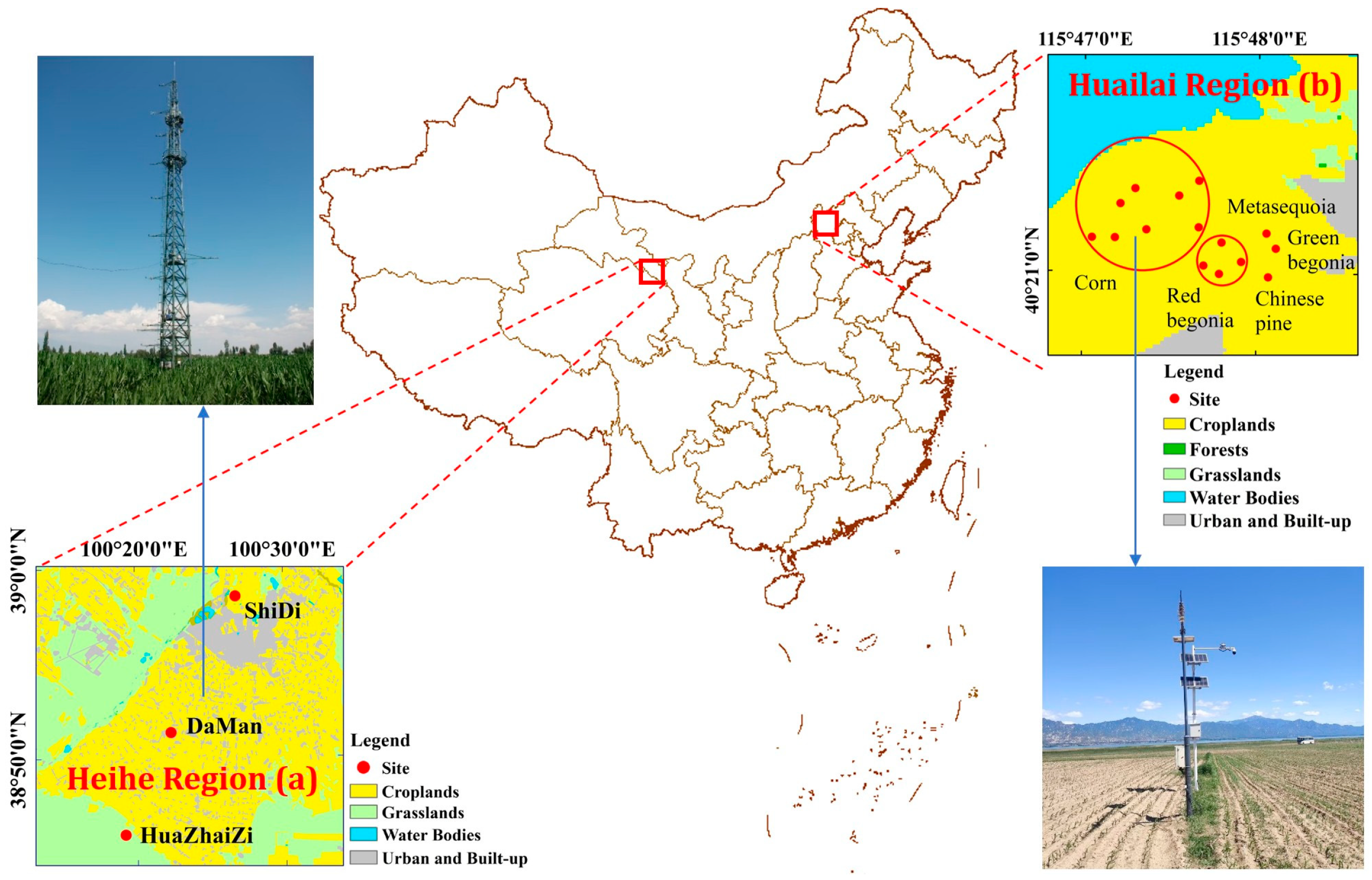
Figure 1. Geographical location of Heihe (a) and Huailai (b) regions in Gansu and Hebei provinces, respectively.
Remotesensing 17 03803 g001
Figure 2. Graphical framework of LST retrieval using: (a) SFTL and (b) SW Algorithm.
Remotesensing 17 03803 g002
Figure 3. General concept of TL for tabulate datasets involving six features.
Remotesensing 17 03803 g003
Figure 4. Feature correlation matrix.
Remotesensing 17 03803 g004
Figure 5. Metrics of LST retrieval performance: (a) the SW algorithm, (b) NN and tree-based models for the Heihe dataset, and (c) NN and tree-based models for the Huailai dataset.
Remotesensing 17 03803 g005
Figure 6. Loss function curves for all folds and true vs. predicted LST values in pre-training NN models.
Remotesensing 17 03803 g006
Figure 7. Ablation of fine-tuning strategies and cross-site generalization for LST estimation. Columns present model/strategy combinations—TrF, DNN, CNN, and tree-based baselines (RF, LGBM) under full, head, gradual, adapter, and LoRA updates—while rows report performance metrics: RMSE (K), R2, MAPE %, and residual distributions (K). Blue bars correspond to Huailai (in-domain, fine-tuned site), and orange bars correspond to Heihe (cross-site generalization).
Remotesensing 17 03803 g007
Figure 8. Ablation of fine-tuning strategies and cross-site generalization for LST estimation. Columns present model/strategy combinations—TrF, DNN, CNN, and tree-based baselines (RF and LGBM) under full, head, gradual, adapter, and LoRA updates—while rows report performance metrics: RMSE (K), R2, MAPE %, and residual distributions (K). Blue bars correspond to Heihe (in-domain, fine-tuned site), and orange bars correspond to Huailai (cross-site generalization).
Remotesensing 17 03803 g008
Figure 9. Real GF5-02 VIMI TIR image LST retrieval for the Huailai region using the best model/strategies and validation via corresponding (spatio-temporally) in situ data: (a) residual distributions across TrF and DNN strategies; (b) GF5-02 VIMI LST retrieval maps for five observation dates; (c) aggregated site-level metrics (R2, RMSE, MAE, MAPE); and (d) pointwise true–predicted LST agreement by surface type.
Remotesensing 17 03803 g009
Figure 10. Real GF5-02 VIMI TIR image LST retrieval for the Heihe region using the best model/strategies and validation via corresponding (spatio-temporally) in situ data: (a) residual distributions across TrF/head and CNN/lora model/strategies; (b) GF5-02 VIMI LST retrieval maps for five observation dates; (c) aggregated site-level metrics (R2, RMSE, MAE, MAPE); and (d) pointwise true–predicted LST agreement by surface type.
Remotesensing 17 03803 g010
Table 1. Details of ground measurement sites.
NetworkSiteLongitudeLatitudeSurface Type
HeiheDaMan100.372238.8556Corn
HuaZhaizi100.320138.7659Desert Steppe
ShiDi100.446438.9751Weed
HuailaiRed begonia1115.796640.3522Shrub
Red begonia2115.798540.3508
Red begonia3115.794940.3505
Red begonia4115.796440.3499
Green begonia115.801840.3518
Metasequoia115.800940.3529Forest
Chinese pine115.801140.3497
Corn1115.784240.3525Crop
Corn2115.786440.3525
Corn3115.786940.3550
Corn4115.788340.3561
Corn5115.794440.3567
Corn6115.792540.3556
Corn7115.794440.3533
Corn8115.789440.3531
Table 2. Descriptions of GF5-02 VIMI channels.
BandSpectral RangeBandSpectral Range
B1
B2
B3
B4
B5
B6
0.45–0.52 μm
0.52–0.60 μm
0.62–0.68 μm
0.76–0.86 μm
1.6–1.8 μm
2.1–2.4 μm
B7
B8
B9
B10
B11
B12
3.5–3.9 μm
4.8–5.0 μm
8.0–8.4 μm
8.4–8.9 μm
10.4–11.3 μm
11.4–12.5 μm
Table 3. Pre-training models’ hyperparameters (training on simulated dataset).
ModelHyperparametersVariablesTop Features
(Permutation Importance)
TrFhidden_dim = 128, num_layers = 6, dropout = 0.3, num_head = 8water vapor content (WVC), brightness temperature (BT) for channel-11&12, land surface emissivity (LSE) for channel-11&12, and
WVC × ΔBT
BT_11, BT_12, WVC × ΔBT
DNNhidden_dim = 128, num_layers = 6, dropout = 0.3BT_11, BT_12, WVC × ΔBT
CNNhidden_dim = 128, dropout = 0.3BT_11, BT_12, WVC
RFn_estimators = 300, max_depth = 30, max_features = ‘sqrt’, min_samples_split = 2, min_samples_leaf = 1BT_11, BT_12, WVC
LGBMn_estimators = 300, max_depth = 30, num_leaves = 70, learning_rate = 0.1, feature_fraction = 0.8, bagging_fraction = 0.7, lambda_l1 = 0, lambda_l2 = 1.0BT_11, WVC, BT_12
Table 4. Accuracy metrics of pre-training models on simulated dataset.
ModelAvg CV RSME (K)Avg CV R2Test RMSE (K)Test MAE (K)Test R2Top Features
(Permutation Importance)
TrF1.210.99800.9990.60000.9990BT_11, BT_12, WVC × ΔBT
DNN0.960.99900.9360.51820.9991BT_11, BT_12, WVC × ΔBT
CNN1.420.99801.2800.81090.9983BT_11, BT_12, WVC
RF0.290.99990.2960.16000.9999BT_11, BT_12, WVC
LGBM0.4160.99980.4100.29200.9998BT_11, WVC, BT_12
Table 5. Summary of metrics for fine-tuning on Huailai (generalization on Heihe).
ModelStrategyHuailai
RMSE(K)
Huailai
R2
Huailai
MAPE (%)
Heihe
RMSE (K)
Heihe
R2
Heihe
MAPE (%)
TrFfull2.500.970.724.690.901.31
head3.080.950.963.780.931.10
gradual3.330.950.915.070.881.45
adapter3.340.940.944.330.911.30
lora3.000.950.933.200.950.96
DNNfull2.670.970.782.960.960.88
head3.680.931.127.920.701.98
gradual2.620.970.762.890.960.83
adapter3.240.930.993.660.941.07
lora4.380.901.269.180.592.34
CNNfull3.300.950.958.760.642.25
head3.610.941.104.910.891.45
gradual3.260.950.936.570.801.78
adapter2.920.960.875.360.871.44
lora3.360.940.9611.550.382.91
RFdefault2.330.970.615.320.831.59
LGBMdefault3.070.950.775.970.801.79
Table 6. Summary of metrics for fine-tuning on Heihe (generalization on Huailai).
ModelStrategyHeihe
RMSE (K)
Heihe
R2
Heihe
MAPE (%)
Huailai
RMSE (K)
Huailai
R2
Huailai
MAPE (%)
TrFfull2.200.960.595.590.821.52
head2.560.940.883.340.940.92
gradual2.390.950.696.070.801.68
adapter2.690.940.864.500.891.31
lora2.120.960.643.410.940.59
DNNfull2.830.930.776.690.741.67
head3.530.890.995.410.811.36
gradual2.760.940.815.980.801.61
adapter2.750.930.885.680.811.33
lora3.120.920.995.590.801.46
CNNfull3.550.891.005.770.771.54
head3.310.901.034.790.881.33
gradual3.490.891.105.450.841.49
adapter3.400.901.045.270.851.46
lora3.270.911.083.670.931.04
RFdefault2.570.940.744.040.911.14
LGBMdefault3.630.891.216.560.771.84
Table 7. Huailai and Heihe GF5-02 VIMI real image LST retrieval accuracy results across the best model/strategies.
RegionBest
Model/Strategy
RMSE (K)R2MAE (K)MAPE (%)Bias (K)Valid Sample (n)
HuailaiTrF/head3.500.923.261.173.0371
TrF/lora3.270.933.001.082.6471
DNN/full2.910.952.450.882.1371
DNN/gradual2.660.962.240.801.7671
HeiheTrF/head2.500.872.220.790.4211
TrF/lora2.240.901.810.64−0.1411
CNN/lora2.370.881.820.650.9911
Disclaimer/Publisher’s Note: The statements, opinions and data contained in all publications are solely those of the individual author(s) and contributor(s) and not of MDPI and/or the editor(s). MDPI and/or the editor(s) disclaim responsibility for any injury to people or property resulting from any ideas, methods, instructions or products referred to in the content.